


Impact statement
This study demonstrates that spanwise-invariant periodic roughness configurations can effectively delay boundary-layer transition in swept-wing flows dominated by cross-flow instability (CFI). By systematically varying roughness geometry – height, width and chordwise spacing – optimal configurations are identified that extend laminar flow by up to 10 % of the aerofoil chord. Under both idealised and realistic surface conditions with randomised roughness, infrared thermography and velocity-field measurements reveal suppressed CFI amplitudes and altered spanwise spectral content. The results show up to a 17 % reduction in chordwise growth of instability modes. Combining roughness strip arrays with discrete roughness elements (DREs) further enhances control, demonstrating scalability to practical aerodynamic conditions. These findings establish a foundation for passive flow-control strategies that delay transition, offering a robust and low-cost path to improved aerodynamic efficiency in real-flight applications.
1. Introduction
On a swept wing subject to favourable pressure gradient, laminar to turbulent transition is governed by cross-flow instabilities (CFIs) which, in low free-stream turbulence environments, manifest as stationary, co-rotating vortices, closely aligned with the free-stream direction (Bippes Reference Bippes1999; Saric et al. Reference Saric, Reed and White2003; Serpieri & Kotsonis Reference Serpieri and Kotsonis2016). The onset and evolution of stationary CFIs are highly sensitive to surface roughness (Müeller & Bippes Reference Müeller and Bippes1989; Deyhle & Bippes Reference Deyhle and Bippes1996; Radeztsky et al. Reference Radeztsky, Reibert and Saric1999; Saric et al. Reference Saric, Reed and White2003). To induce a monochromatic CFI mode, artificial forcing with a periodic array of discrete roughness elements (DREs) parallel to the leading edge has often been employed (Radeztsky et al. Reference Radeztsky, Reibert and Saric1999; Saric et al. Reference Saric, Reed and White2003; Serpieri & Kotsonis Reference Serpieri and Kotsonis2016). At the same time, Saric et al. (Reference Saric, Carrillo and Reibert1998) demonstrated that sub-critical forcing (using a DRE array whose wavelength is shorter than the critical CFI wavelength, $\lambda _{\mathrm{crit}}$
) can inhibit the growth of the most unstable modes and delay laminar-to-turbulent transition.
$\lambda _{\mathrm{crit}}$
) can inhibit the growth of the most unstable modes and delay laminar-to-turbulent transition.
Previous studies have demonstrated that control methods built on wave superposition principles can successfully control boundary layers for which transition is dominated either by Tollmien–Schlichting (TS) waves (e.g. Milling Reference Milling1981; Tol et al. Reference Tol, de Visser and Kotsonis2019 b) or by CFI (e.g. Wassermann & Kloker Reference Wassermann and Kloker2000; Zoppini et al. Reference Zoppini, Michelis, Ragni and Kotsonis2022 a). In both cases, during the initial exponential growth phase, modes develop independently from each other (i.e. free from non-linear interactions (Bippes Reference Bippes1999; Saric et al. Reference Saric, Reed and White2003; Schlichting & Gersten Reference Schlichting and Gersten2017; Schubauer & Skramstad Reference Schubauer and Skramstad1947)). Therefore, artificially introduced monochromatic disturbances with optimal amplitude and phase shift can be employed without causing significant mode coupling, effectively damping instability growth. In two-dimensional (2-D) scenarios, this has led to the development of adaptive control systems capable of damping TS waves at various locations (Baumann et al. Reference Baumann, Sturzebecher and Nitsche2000; Ladd Reference Ladd1990; Sturzebecher & Nitsche Reference Sturzebecher and Nitsche2003; Tol et al. Reference Tol, Kotsonis and Visser2019 a). In contrast, in three-dimensional (3-D) scenarios, upstream flow deformation (UFD) techniques are implemented in combination with classical BL suction to optimise the location, arrangement and strength of multiple suction orifices, inhibiting primary CFI growth and delaying secondary instabilities (Friederich & Kloker Reference Friederich and Kloker2012; Messing & Kloker Reference Messing and Kloker2010).
Recent investigations have explored the use of passive surface-embedded resonators for controlling TS waves relying either on the excitation of elastic waves within the sub-surface (e.g. Barnes et al. Reference Barnes, Willey, Rosenberg, Medina and Juhl2021; Hussein et al. Reference Hussein, Biringen, Bilal and Kucala2015; Park et al. Reference Park, Hristov, Balasubramanian, Goza, Ansell and Matlack2022; Michelis et al. Reference Michelis, Putranto and Kotsonis2023 b) or the acoustic response of Helmholtz resonators (Michelis et al. Reference Michelis, de Koning and Kotsonis2023 a). The frequency dispersion of the aforementioned resonators can be tailored accordingly such that the interface interferes constructively or destructively with the TS waves, leading to the formation of pass bands or stop bands respectively. While the TS attenuation achieved is modest, the localised scattering effect (Dong & Wu Reference Dong and Wu2016; Xu et al. Reference Xu, Sherwin, Hall and Wu2016) suggests that a properly tuned series of such devices could significantly enhance overall control capabilities over the surface.
Drawing inspiration from the above, to attenuate the development of CFI in a 3-D boundary layer, a passive laminar flow control technique based on the application of a streamwise series of DRE arrays with optimal amplitude and phase arrangement has been investigated by Zoppini et al. (Reference Zoppini, Michelis, Ragni and Kotsonis2022 a). These surface roughness modifications introduce velocity disturbance systems that destructively interfere with the developing CFI through a wave superposition process, significantly reducing its amplitude and delaying BL transition. However, the potential of the proposed cancellation technique is limited by its strong sensitivity to external disturbances, particularly in scenarios with enhanced distributed surface roughness. This behaviour is mostly attributed to the lack of control on the phase shift between pre-existing CFI and the introduced velocity disturbances, resulting in the persistence of residual small-wavelength CFI modes in the boundary layer. In a similar vein, Ivanov et al. (Reference Ivanov, Mischenko and Ustinov2018) reported that oblique surface non-uniformities on a swept wing can either amplify or attenuate the growth of cross-flow vortices, depending on their orientation relative to the leading edge. Specifically, stabilisation occurs when the non-uniformities are aligned parallel to the leading edge. Furthermore, a direct correlation was observed between the number of non-uniformities and the magnitude of the stabilising or destabilising effect, with stronger effects arising as their number increases.
Despite these advancements, to the authors’ best knowledge, other than the aforementioned works, no attempts have been made to stabilise stationary CFI using arrays of periodic units in 3-D BL scenarios, specifically focussing on possible scattering behaviour. This study aims to fill this gap by experimentally investigating the interaction between stationary CFI on a swept wing BL and a spanwise-invariant roughness strip array (SA). Various design parameters are explored to optimise the roughness geometry, with a primary focus on the effect of the array periodicity on BL development. The effectiveness of the SA is evaluated in both a boundary layer forced by a reference DRE array as well as in the presence of randomised distributed roughness (Kendall Reference Kendall1981; Suryanarayanan et al. Reference Suryanarayanan, Goldstein, Berger, White and Brown2020; Zoppini et al. Reference Zoppini, Michelis, Ragni and Kotsonis2022
a). The former results in the development of monochromatic CFI with periodicity corresponding to the DRE forcing wavelength, spanning from sub-critical $(\lambda \lt \lambda _{\mathrm{crit}})$
, critical
$(\lambda \lt \lambda _{\mathrm{crit}})$
, critical $(\lambda =\lambda _{\mathrm{crit}})$
to super-critical
$(\lambda =\lambda _{\mathrm{crit}})$
to super-critical $(\lambda \gt \lambda _{\mathrm{crit}})$
. Conversely, the latter induces more realistic conditions, reflecting a rougher wing surface finish, and leads to a BL with broader spectral content, including the simultaneous development of various CFI modes.
$(\lambda \gt \lambda _{\mathrm{crit}})$
. Conversely, the latter induces more realistic conditions, reflecting a rougher wing surface finish, and leads to a BL with broader spectral content, including the simultaneous development of various CFI modes.
2. Methodology
2.1. Wind tunnel and wing model
The presented work is carried out in the low speed Low Turbulence Tunnel (LTT) of TU Delft ( $T_u/U_\infty \simeq {0.025}\,{\%},$
in the range
$T_u/U_\infty \simeq {0.025}\,{\%},$
in the range ${25}$
–
${25}$
– ${60}\,\mathrm{ms}^{-1}$
, bandpassed between 2 Hz and 5000 Hz, Serpieri Reference Serpieri2018), on a constant-chord (
${60}\,\mathrm{ms}^{-1}$
, bandpassed between 2 Hz and 5000 Hz, Serpieri Reference Serpieri2018), on a constant-chord ( $c_X={1.27}{\mathrm{m}},$
along
$c_X={1.27}{\mathrm{m}},$
along $X$
) swept (
$X$
) swept ( ${45}^\circ$
) wing model (M3J, Serpieri & Kotsonis Reference Serpieri and Kotsonis2015; Serpieri Reference Serpieri2018) with smooth surface
${45}^\circ$
) wing model (M3J, Serpieri & Kotsonis Reference Serpieri and Kotsonis2015; Serpieri Reference Serpieri2018) with smooth surface $({R}_q = {0.2}\,{{\unicode{x03BC}}\mathrm{m}})$
. The model is designed to ensure that stationary CFI dominates the BL evolution and transition, providing a favourable pressure gradient up to 65 % chord. Measurements are performed on the pressure side of the wing model at angle of attack
$({R}_q = {0.2}\,{{\unicode{x03BC}}\mathrm{m}})$
. The model is designed to ensure that stationary CFI dominates the BL evolution and transition, providing a favourable pressure gradient up to 65 % chord. Measurements are performed on the pressure side of the wing model at angle of attack $\alpha = {-3.4}^\circ$
and Reynolds number
$\alpha = {-3.4}^\circ$
and Reynolds number $\mathrm{Re}_{c_x} = 2.17 \times 10^6$ $(U_\infty = {25.6}\,\mathrm{ms}^{-1})$
. An overview of the experimental set-up is shown in Figure 1. Two different coordinate systems are used throughout this work: the first is integral to the wind tunnel floor, with spatial components
$(U_\infty = {25.6}\,\mathrm{ms}^{-1})$
. An overview of the experimental set-up is shown in Figure 1. Two different coordinate systems are used throughout this work: the first is integral to the wind tunnel floor, with spatial components $X, Y, Z$
and velocity components
$X, Y, Z$
and velocity components $U, V, W$
, and is employed for the analysis of the acquired infrared images; the second is a wall-attached, curvilinear, coordinate system, integral to the swept wing, with the
$U, V, W$
, and is employed for the analysis of the acquired infrared images; the second is a wall-attached, curvilinear, coordinate system, integral to the swept wing, with the $z$
-axis aligned to the leading edge, while the
$z$
-axis aligned to the leading edge, while the $x\text{-axis}$
and
$x\text{-axis}$
and $y\text{-axis}$
are parallel and normal to the local surface tangent, respectively. Corresponding body-fitted velocity components
$y\text{-axis}$
are parallel and normal to the local surface tangent, respectively. Corresponding body-fitted velocity components $u, v, w$
are extracted from particle image velocimetry (PIV) measurements. At this angle of attack, spanwise pressure gradient uniformity was found to be excellent (Serpieri & Kotsonis Reference Serpieri and Kotsonis2015); hence, no wall liners were necessary to treat the wind tunnel walls (see e.g. Deyhle & Bippes Reference Deyhle and Bippes1996).
$u, v, w$
are extracted from particle image velocimetry (PIV) measurements. At this angle of attack, spanwise pressure gradient uniformity was found to be excellent (Serpieri & Kotsonis Reference Serpieri and Kotsonis2015); hence, no wall liners were necessary to treat the wind tunnel walls (see e.g. Deyhle & Bippes Reference Deyhle and Bippes1996).
Schematic of the experimental set-up (not to scale) with the various roughness configurations; strip array (SA) and distributed roughness patch (DRP). The right panel depicts the aerofoil shape along $X$
(to scale) and the corresponding pressure coefficient at the experiment conditions.
$X$
(to scale) and the corresponding pressure coefficient at the experiment conditions.

2.2. Surface roughness features
2.2.1. Discrete roughness element (DRE) arrays
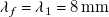
At the aforementioned experimental conditions, linear stability theory predictions based on in-house solutions of the Orr–Sommerfeld equation (Mack Reference Mack1984) and previous work from the authors (Serpieri & Kotsonis Reference Serpieri and Kotsonis2015) confirm that the critical modes lie in the range of 8–10 mm for a smooth wing without surface modifications. Discrete roughness element (DRE) arrays are applied at $x_{\mathrm{DRE}}/c={0.02}{}$
to ensure the development of a monochromatic CFI mode (e.g. Radeztsky et al. Reference Radeztsky, Reibert and Saric1999; Saric et al. Reference Saric, Reed and White2003). A critical DRE array with element inter-spacing of
$x_{\mathrm{DRE}}/c={0.02}{}$
to ensure the development of a monochromatic CFI mode (e.g. Radeztsky et al. Reference Radeztsky, Reibert and Saric1999; Saric et al. Reference Saric, Reed and White2003). A critical DRE array with element inter-spacing of $\lambda _f = \lambda _1 = {8}{\,\mathrm{mm}}$
provides the reference baseflow BL for the majority of the presented cases, ensuring that the CFI attains measurable amplitude downstream of
$\lambda _f = \lambda _1 = {8}{\,\mathrm{mm}}$
provides the reference baseflow BL for the majority of the presented cases, ensuring that the CFI attains measurable amplitude downstream of $x/c={0.1}{}$
. Nevertheless, based on linear stability analysis (Figure 2), the SA is anticipated to also interact with cross-flow instabilities of wavelengths other than the forced critical one. To confirm if this is the case, sub-critical
$x/c={0.1}{}$
. Nevertheless, based on linear stability analysis (Figure 2), the SA is anticipated to also interact with cross-flow instabilities of wavelengths other than the forced critical one. To confirm if this is the case, sub-critical $(\lambda _f={6}{\,\mathrm{mm}})$
, near-critical
$(\lambda _f={6}{\,\mathrm{mm}})$
, near-critical $(\lambda _f={7}{\,\mathrm{mm}})$
and super-critical
$(\lambda _f={7}{\,\mathrm{mm}})$
and super-critical $(\lambda _f={10}{\,\mathrm{mm}})$
baseflow configurations are also considered.
$(\lambda _f={10}{\,\mathrm{mm}})$
baseflow configurations are also considered.
Linear stability analysis amplification factor $(N)$
of the unforced BL for a set of stationary modes with
$(N)$
of the unforced BL for a set of stationary modes with $\lambda$
ranging from 4 mm to 12 mm.
$\lambda$
ranging from 4 mm to 12 mm.
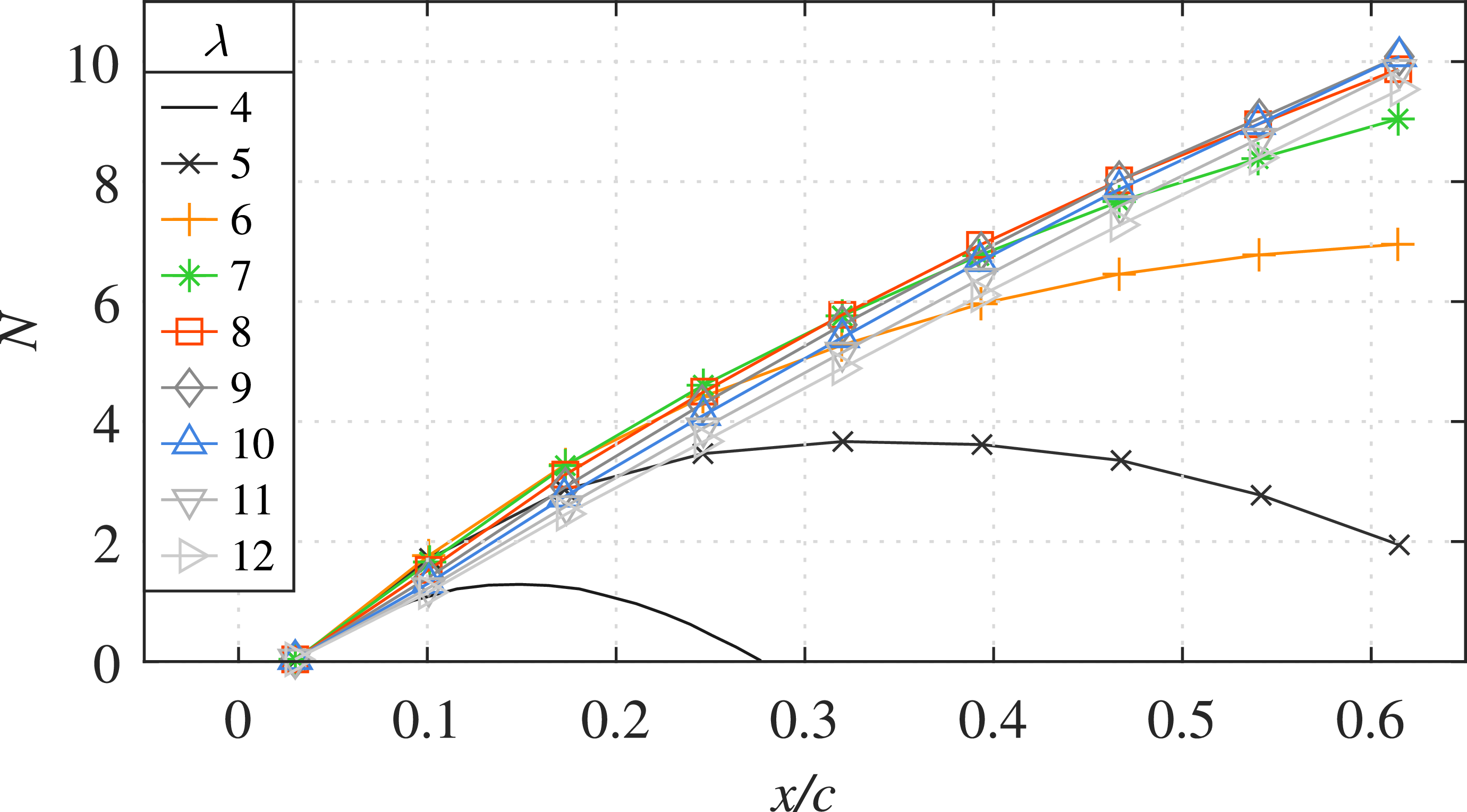
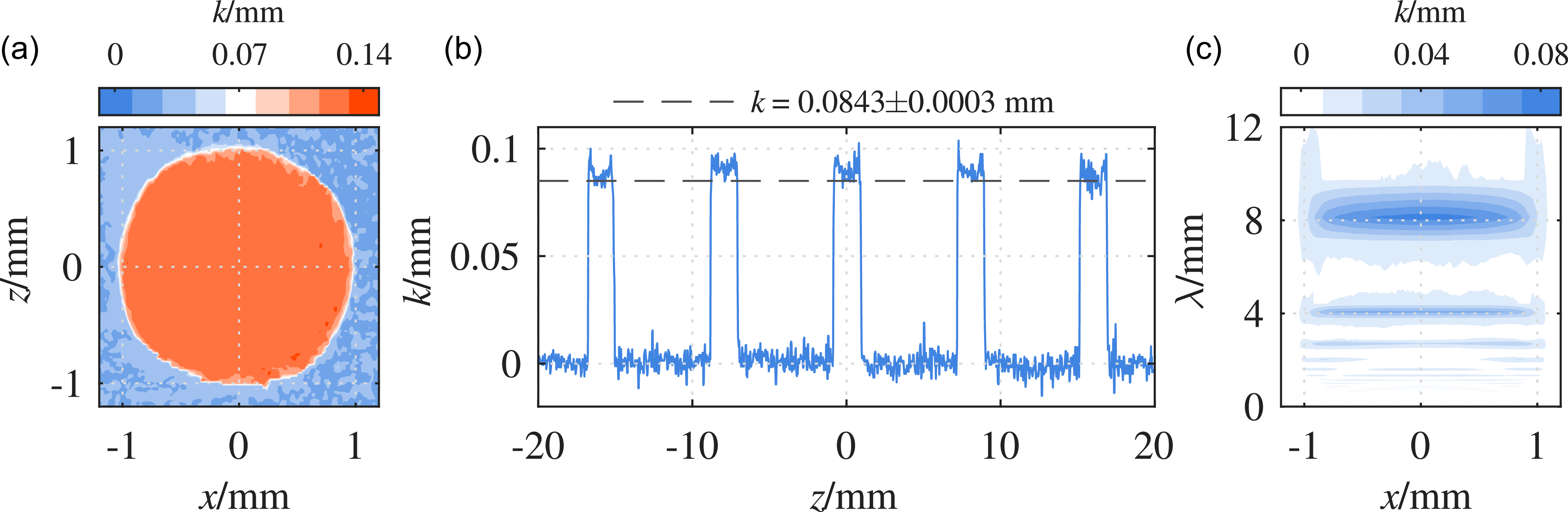
All DRE arrays (see Table 1 for properties) are manufactured in-house and geometrically characterised as described by Zoppini (Reference Zoppini2023), by knife cutting a PVC foil with nominal height of $k={70}\,{{\unicode{x03BC}}\mathrm{m}}$
. Each DRE is designed to feature a cylindrical shape with diameter
$k={70}\,{{\unicode{x03BC}}\mathrm{m}}$
. Each DRE is designed to feature a cylindrical shape with diameter $d={2}\,\mathrm{mm}$
. To ensure no major shape and height variations occur due to the manufacturing process, a statistical characterisation of their geometric properties is performed. Sub-samples of the arrays are scanned with a scanCONTROL 30xx profilometer, operating with a semiconductor laser with a 405 nm wavelength and
$d={2}\,\mathrm{mm}$
. To ensure no major shape and height variations occur due to the manufacturing process, a statistical characterisation of their geometric properties is performed. Sub-samples of the arrays are scanned with a scanCONTROL 30xx profilometer, operating with a semiconductor laser with a 405 nm wavelength and ${1.5}\,{\unicode{x03BC}\mathrm{m}}$
reference resolution. The data acquisition and processing is described by Zoppini et al. (Reference Zoppini, Westerbeek, Ragni and Kotsonis2022
b), resulting in an effective element height of
${1.5}\,{\unicode{x03BC}\mathrm{m}}$
reference resolution. The data acquisition and processing is described by Zoppini et al. (Reference Zoppini, Westerbeek, Ragni and Kotsonis2022
b), resulting in an effective element height of $k={0.0843\pm 0.0003}\,\mathrm{mm}$
and diameter
$k={0.0843\pm 0.0003}\,\mathrm{mm}$
and diameter $d={2.03\pm 0.0013}\,\mathrm{mm}$
for the current application (Figure 3).
$d={2.03\pm 0.0013}\,\mathrm{mm}$
for the current application (Figure 3).
2.2.2. Distributed surface roughness patches (DRPs)
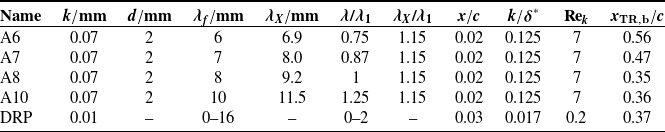
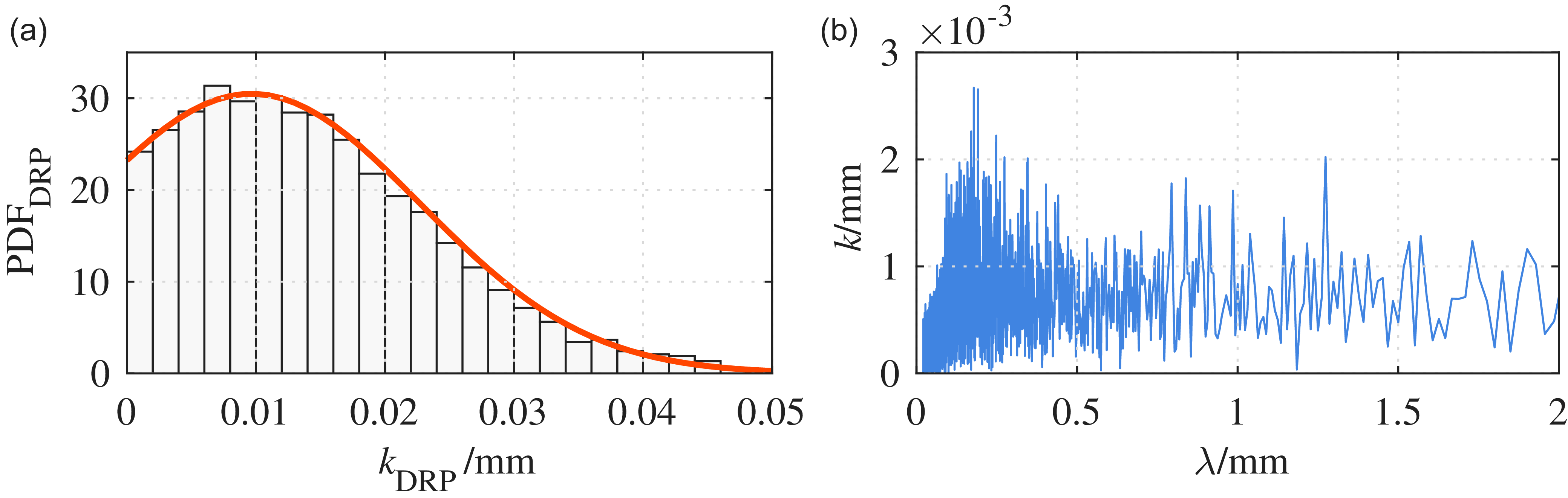
Typically, the surface finishing of commercial air vehicles results in a distributed surface roughness with an average height of $\simeq {11}\,{{\unicode{x03BC}}\mathrm{m}}$
(Boeing 2013). Therefore, to mimic background surface roughness, distributed roughness patches (fine silicon carbide) are applied on the wing, resulting in a random distribution of local roughness peaks, as characterised by Zoppini et al. (Reference Zoppini, Michelis, Ragni and Kotsonis2022
a). The resulting DRP average height is
$\simeq {11}\,{{\unicode{x03BC}}\mathrm{m}}$
(Boeing 2013). Therefore, to mimic background surface roughness, distributed roughness patches (fine silicon carbide) are applied on the wing, resulting in a random distribution of local roughness peaks, as characterised by Zoppini et al. (Reference Zoppini, Michelis, Ragni and Kotsonis2022
a). The resulting DRP average height is $k_{\mathrm{DRP}} \simeq 0.010\pm 0.001\,\mathrm{mm}$
, with local peak heights reaching a maximum value of approximately 0.04 mm (Figure 4a). The DRP amplitude distribution is characterised by a broadband spanwise spatial content in the range of
$k_{\mathrm{DRP}} \simeq 0.010\pm 0.001\,\mathrm{mm}$
, with local peak heights reaching a maximum value of approximately 0.04 mm (Figure 4a). The DRP amplitude distribution is characterised by a broadband spanwise spatial content in the range of $0{-}2 \lambda _1$
(Figure 4b). Hence, it is expected that the DRP will excite a set of CFI modes with various spanwise wavelengths within the same range, resulting in a BL containing simultaneously developing small wavelength CFI (Saric et al. Reference Saric, Carpenter and Reed2011; Zoppini et al. Reference Zoppini, Michelis, Ragni and Kotsonis2022
a). Throughout this work, the cases combining elevated background roughness and other roughness manipulations (i.e. DRP and SA or DRP, DRE and SA) feature the same DRP located at
$0{-}2 \lambda _1$
(Figure 4b). Hence, it is expected that the DRP will excite a set of CFI modes with various spanwise wavelengths within the same range, resulting in a BL containing simultaneously developing small wavelength CFI (Saric et al. Reference Saric, Carpenter and Reed2011; Zoppini et al. Reference Zoppini, Michelis, Ragni and Kotsonis2022
a). Throughout this work, the cases combining elevated background roughness and other roughness manipulations (i.e. DRP and SA or DRP, DRE and SA) feature the same DRP located at $x_{\mathrm{DRP}}/c=0.03$
(see Figure 1).
$x_{\mathrm{DRP}}/c=0.03$
(see Figure 1).
Nominal geometric parameters of the DRE arrays and DRP and the respective transition location
Statistical characterisation of a DRE array: (a) height map of a representative DRE element; (b) slice of the height map along the centreline of the DRE array; (c) spatial spectrum of the DRE array.
Statistical characterisation of a sample DRP: (a) typical histogram of a DRP heightmap showcasing the distribution of roughness height; (b) a representative wavelength spectrum of the DRP.
2.2.3. Spanwise-invariant roughness Strip Arrays (SAs)
Spanwise-uniform roughness strip arrays (SAs) are designed to attenuate the CFI developing in the reference BL. Unlike traditional 2-D BL control methods, this approach targets stationary, wave-like CFI patterns along the chord-wise (streamwise) direction, matching the instability’s spatial periodicity. This is reminiscent of the work by Justiniano et al. (Reference Justiniano, Brown, White, Suryanarayanan and Goldstein2024) and Suryanarayanan et al. (Reference Suryanarayanan, Goldstein, Berger, White and Brown2020) on distributed roughness shielding in unswept flows dominated by streaky structures. The SA, therefore, operates parallel to the instability propagation direction, contrasting with transverse (wall-normal) approaches for Tollmien–Schlichting wave attenuation (Hussein et al. Reference Hussein, Biringen, Bilal and Kucala2015; Michelis et al. Reference Michelis, de Koning and Kotsonis2023 a).
Several considerations are factored in the SA design. For representative measurements, they must be applied in the region of the BL where CFIs are already exponentially amplified, yet not saturated, as to avoid the insurgence of secondary instabilities and laminar breakdown. Based on previous investigations (Zoppini et al. 2022a), for the present set-up, the chord location combining these two requirements is ${x/c} = 0.125$
. For similarity with the employed DRE arrays, the individual strips are designed such that they are parallel to the leading edge, with predefined nominal height and width of
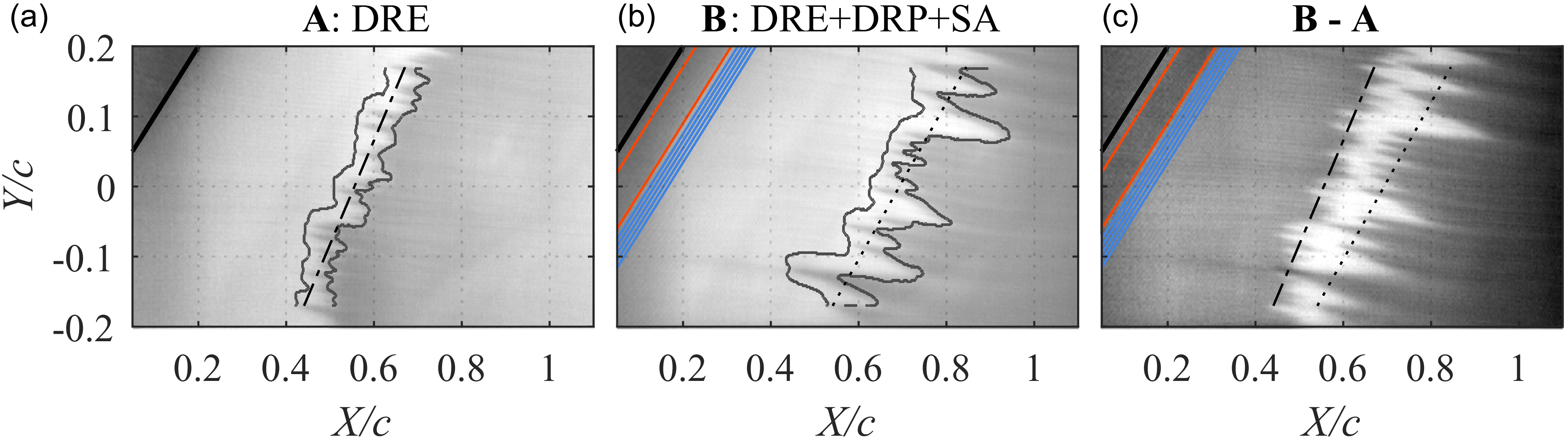
${x/c} = 0.125$
. For similarity with the employed DRE arrays, the individual strips are designed such that they are parallel to the leading edge, with predefined nominal height and width of ${k_{\mathrm{SA}}} = {0.07}{\,\mathrm{mm}}$
and
${k_{\mathrm{SA}}} = {0.07}{\,\mathrm{mm}}$
and ${w_{\mathrm{SA}}} = {2}\,\mathrm{mm}$
, respectively. The SA location (i.e.
${w_{\mathrm{SA}}} = {2}\,\mathrm{mm}$
, respectively. The SA location (i.e. $x_{\mathrm{SA}}/c$
) is defined as the location of the first strip on the wing (set to
$x_{\mathrm{SA}}/c$
) is defined as the location of the first strip on the wing (set to $x/c={0.125}{}$
), while the number of strip units in each SA
$x/c={0.125}{}$
), while the number of strip units in each SA $(N_{\mathrm{SA}})$
is applied with set streamwise periodicity. This characteristic wavelength is set to match the streamwise wavelength of the dominant CFI
$(N_{\mathrm{SA}})$
is applied with set streamwise periodicity. This characteristic wavelength is set to match the streamwise wavelength of the dominant CFI $(\lambda _X)$
, which is determined during preliminary IR investigation of the DRE-forced BL to be
$(\lambda _X)$
, which is determined during preliminary IR investigation of the DRE-forced BL to be ${9.2}\,\mathrm{mm}$
at
${9.2}\,\mathrm{mm}$
at $x/c={0.125}{}$
.
$x/c={0.125}{}$
.
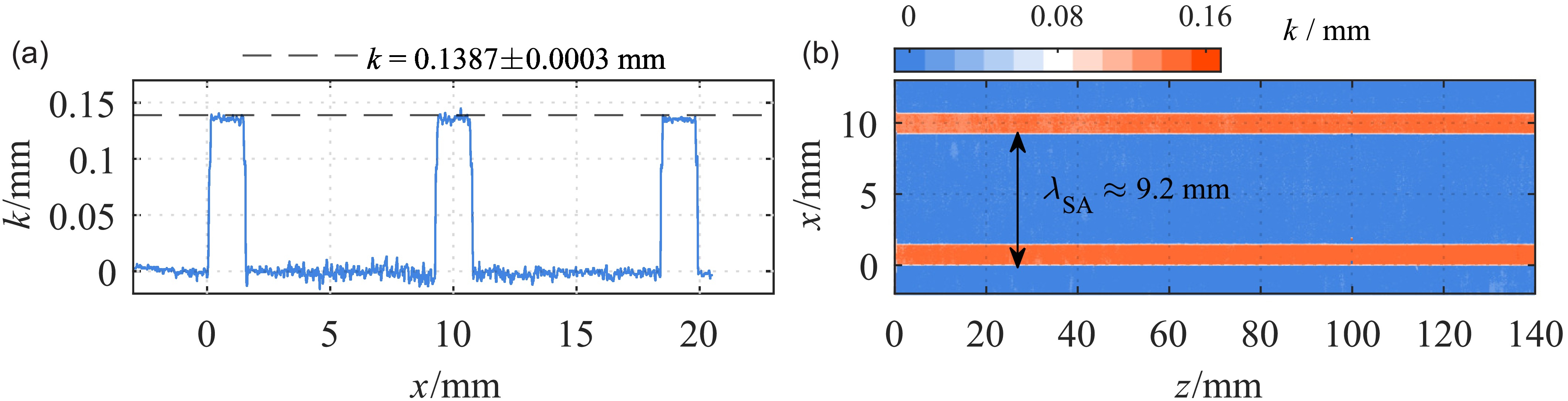
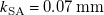
SAs are manufactured in-house by knife cutting PVC foils of nominal height between 0.07 mm and 0.17 mm. The procedure is analogous to the DRE cutting, with each SA being produced as a single piece to be pasted on the wing. A reference sample is laser-scanned to assess the effective geometry, of nominal values for height, width and periodicity of $k_{\mathrm{SA}}={0.14}\,\mathrm{mm}$
,
$k_{\mathrm{SA}}={0.14}\,\mathrm{mm}$
, $w_{\mathrm{SA}}={2}\,\mathrm{mm}$
and
$w_{\mathrm{SA}}={2}\,\mathrm{mm}$
and $\lambda _{\mathrm{SA}}={9.2}\,\mathrm{mm}$
, respectively (Figure 5).
$\lambda _{\mathrm{SA}}={9.2}\,\mathrm{mm}$
, respectively (Figure 5).
Characterisation of the roughness strip array: (a) representative slice of strip height; (b) height map of two representative strips.
2.3. Measurement techniques
2.3.1. Infrared thermography
Infrared (IR) thermography employs radiometric sensors located outside of the wind tunnel test section, allowing non-intrusive imaging of the wing surface temperature. Based on the Reynolds’ analogy (Reynolds, Reference Reynolds1883), higher temperature regions in the IR image are associated with laminar flow, while lower temperature regions correspond to turbulent flow (Bippes Reference Bippes1999; Dagenhart & Saric Reference Dagenhart and Saric1999; Serpieri Reference Serpieri2018). Therefore, an IR image offers a global overview of the flow field, and provides the location and topology of the BL laminar-to-turbulent transition.
In the current investigation, an Optris PI640 IR camera images the wing pressure side at the chosen flow conditions (i.e. $\mathrm{Re}_c=2.17\times 10^6$
and
$\mathrm{Re}_c=2.17\times 10^6$
and $\alpha = {-3.4}^\circ$
) for the various roughness configurations considered. The acquired domain is centred at the wing midspan and imaging with spatial resolution of
$\alpha = {-3.4}^\circ$
) for the various roughness configurations considered. The acquired domain is centred at the wing midspan and imaging with spatial resolution of $\simeq {1.7}\,\mathrm{mm \, px}^{-1}$
. Given the stationary nature of the investigated flow features, for each configuration, 80 images are acquired at a frequency of 4 Hz and are averaged to reduce the image-to-noise ratio. The thermal contrast between laminar and turbulent flow regions is enhanced by external surface heating provided by IR-optimised halogen lamps
$\simeq {1.7}\,\mathrm{mm \, px}^{-1}$
. Given the stationary nature of the investigated flow features, for each configuration, 80 images are acquired at a frequency of 4 Hz and are averaged to reduce the image-to-noise ratio. The thermal contrast between laminar and turbulent flow regions is enhanced by external surface heating provided by IR-optimised halogen lamps $(3\times {400}\,\mathrm{W}$
and
$(3\times {400}\,\mathrm{W}$
and $2\times {500}\,\mathrm{W})$
. The model temperature increase occurring throughout the measurement is within 4 % of the measured flow temperature (in K); hence, any effect the BL transition location is negligible, as also observed in previous experimental investigations (Lemarechal et al. Reference Lemarechal, Costantini, Klein, Kloker, Würz, Kurz, Streit and Schaber2019). The averaged IR images (Figure 6) are geometrically mapped to the tunnel-attached reference system,
$2\times {500}\,\mathrm{W})$
. The model temperature increase occurring throughout the measurement is within 4 % of the measured flow temperature (in K); hence, any effect the BL transition location is negligible, as also observed in previous experimental investigations (Lemarechal et al. Reference Lemarechal, Costantini, Klein, Kloker, Würz, Kurz, Streit and Schaber2019). The averaged IR images (Figure 6) are geometrically mapped to the tunnel-attached reference system, $X, Y, Z$
, and are post-processed through an in-house developed routine that locally identifies the absolute transition location
$X, Y, Z$
, and are post-processed through an in-house developed routine that locally identifies the absolute transition location $(x_{\mathrm{TR}})$
on the surface of the wing by means of Gabor filtering (Gabor Reference Gabor1946; Michelis et al. Reference Michelis, Head and Colonna2024).
$(x_{\mathrm{TR}})$
on the surface of the wing by means of Gabor filtering (Gabor Reference Gabor1946; Michelis et al. Reference Michelis, Head and Colonna2024).
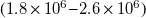
Exemplary infrared images for: (a) DRE forced BL; (b) DRE/DRP/SA forced BL; (c) differential result, the bright area exhibiting the extent of transition delay. Aerofoil leading edge (![]() ); extent of DRP (
); extent of DRP (![]() ); SA units (
); SA units (![]() ); transition region identified with Gabor filtering (
); transition region identified with Gabor filtering (![]() ); linear fit of transition region (
); linear fit of transition region (![]() ,
, ![]() ) that defines
) that defines $x_{\mathrm{TR}}$
along the span.
$x_{\mathrm{TR}}$
along the span.
2.3.2. Planar particle image velocimetry (PIV) and vector field processing
Particle image velocimetry (PIV) is used to locally quantify the BL flow characteristics and its chordwise development under different forcing configurations along the $z{-}y$
plane (i.e. spanwise wall-normal) at a fixed chord location,
$z{-}y$
plane (i.e. spanwise wall-normal) at a fixed chord location, $x/c=0.25$
(Figure 1). The
$x/c=0.25$
(Figure 1). The $z$
and
$z$
and $y$
coordinates are normalised by
$y$
coordinates are normalised by $\lambda _1={8}\,\mathrm{mm}$
and the experimentally determined displacement thickness on the
$\lambda _1={8}\,\mathrm{mm}$
and the experimentally determined displacement thickness on the $z{-}y$
plane at
$z{-}y$
plane at $x/c=0.3$
(
$x/c=0.3$
( $\delta _w^*={0.72}\,\mathrm{mm}$
), respectively. Illumination is provided by a Quantel Evergreen Nd:YAG dual cavity laser (200 mJ per pulse at
$\delta _w^*={0.72}\,\mathrm{mm}$
), respectively. Illumination is provided by a Quantel Evergreen Nd:YAG dual cavity laser (200 mJ per pulse at $\lambda ={532}\,\mathrm{nm}$
). A set of optics is used to transform the beam to a sheet of approximately 1 mm thickness. Imaging is performed with a LaVision Imager camera (sCMOS,
$\lambda ={532}\,\mathrm{nm}$
). A set of optics is used to transform the beam to a sheet of approximately 1 mm thickness. Imaging is performed with a LaVision Imager camera (sCMOS, $2560\times 2160$
pixels, 16-bit,
$2560\times 2160$
pixels, 16-bit, ${6.5}\,{{\unicode{x03BC}}\mathrm{m}}$
pixel pitch) equipped with a 200 mm objective
${6.5}\,{{\unicode{x03BC}}\mathrm{m}}$
pixel pitch) equipped with a 200 mm objective $(f_\# = 8)$
and a
$(f_\# = 8)$
and a $2\times$
tele-converter to attain the field of view (35 mm
$2\times$
tele-converter to attain the field of view (35 mm $\times$
10 mm). Seeding is obtained by dispersing
$\times$
10 mm). Seeding is obtained by dispersing ${0.5}\,{{\unicode{x03BC}}\mathrm{m}}$
droplets of water–glycol mixture through a SAFEX fog generator. Each image pair
${0.5}\,{{\unicode{x03BC}}\mathrm{m}}$
droplets of water–glycol mixture through a SAFEX fog generator. Each image pair $(\Delta t={15}\,{\unicode{x03BC}\mathrm{s}})$
is processed in LaVision Davis 10, employing a 2-frame particle tracking (PTV) algorithm to identify particle trajectories, which are then spatially binned
$(\Delta t={15}\,{\unicode{x03BC}\mathrm{s}})$
is processed in LaVision Davis 10, employing a 2-frame particle tracking (PTV) algorithm to identify particle trajectories, which are then spatially binned $(6 \times {6}\,\mathrm{px^2})$
and converted to a
$(6 \times {6}\,\mathrm{px^2})$
and converted to a $500\times 140$
Cartesian grid with a vector pitch of
$500\times 140$
Cartesian grid with a vector pitch of ${80}\,{{\unicode{x03BC}}\mathrm{m}}$
.
${80}\,{{\unicode{x03BC}}\mathrm{m}}$
.
Time-averaged spanwise and wall-normal velocity fields $(\overline {w}, \overline {v})$
are further processed to extract the main flow features. The spanwise-average of
$(\overline {w}, \overline {v})$
are further processed to extract the main flow features. The spanwise-average of $\overline {w}$
is used to define the baseline mean BL velocity profile
$\overline {w}$
is used to define the baseline mean BL velocity profile $\overline {w}_{\mathrm{b}}$
at
$\overline {w}_{\mathrm{b}}$
at $x/c=0.30$
. This provides an estimate of the free-stream spanwise velocity,
$x/c=0.30$
. This provides an estimate of the free-stream spanwise velocity, $W_\infty$
, indicating that the employed optical set-up and processing resolve the BL up to
$W_\infty$
, indicating that the employed optical set-up and processing resolve the BL up to $\overline {w}=1.4\,\% W_\infty$
, with local uncertainty of 0.6 % within the BL and 0.04 % in the free stream. The
$\overline {w}=1.4\,\% W_\infty$
, with local uncertainty of 0.6 % within the BL and 0.04 % in the free stream. The $\overline {v}$
component is resolved up to
$\overline {v}$
component is resolved up to $\overline {v}=1.4\,\% V_\infty$
, with local uncertainty of 4 % within the BL and 0.04 % in the free stream. By subtracting the
$\overline {v}=1.4\,\% V_\infty$
, with local uncertainty of 4 % within the BL and 0.04 % in the free stream. By subtracting the $\overline {w}_{\mathrm{b}}$
profile from
$\overline {w}_{\mathrm{b}}$
profile from $\overline {w}$
, the disturbance velocity field,
$\overline {w}$
, the disturbance velocity field, $\overline {w}_{\mathrm{d}}$
, is obtained. The standard deviation of
$\overline {w}_{\mathrm{d}}$
, is obtained. The standard deviation of $\overline {w}$
along the spanwise direction can, instead, provide an estimation of the disturbance profile along the
$\overline {w}$
along the spanwise direction can, instead, provide an estimation of the disturbance profile along the $y$
direction,
$y$
direction, $\langle \overline {w}\rangle _z$
(see e.g. Hunt & Saric Reference Hunt and Saric2011; Reibert et al. Reference Reibert, Saric, Carrillo and Chapman1996; Tempelmann et al. Reference Tempelmann, Schrader, Hanifi, Brandt and Henningson2012).
$\langle \overline {w}\rangle _z$
(see e.g. Hunt & Saric Reference Hunt and Saric2011; Reibert et al. Reference Reibert, Saric, Carrillo and Chapman1996; Tempelmann et al. Reference Tempelmann, Schrader, Hanifi, Brandt and Henningson2012).
Spatial fast Fourier transform (FFT) analysis is performed to infer the spectral organisation of the flow field: at each $y$
coordinate, the spanwise
$y$
coordinate, the spanwise $\overline {w}_{\mathrm{d}}$
signal is transformed to the spatial frequency domain, providing information on the modal composition of the developing BL and on the evolution of the individual Fourier modes. Such FFT analysis also provides fundamental information regarding the phase of the individual modes, which is fundamental to establish the SA effect on the flow field. Moreover, the local CFI amplitude
$\overline {w}_{\mathrm{d}}$
signal is transformed to the spatial frequency domain, providing information on the modal composition of the developing BL and on the evolution of the individual Fourier modes. Such FFT analysis also provides fundamental information regarding the phase of the individual modes, which is fundamental to establish the SA effect on the flow field. Moreover, the local CFI amplitude $(A_{\mathrm{int}})$
is estimated following the integral amplitude definition (Downs & White Reference Downs and White2013). More specifically, the disturbance profiles
$(A_{\mathrm{int}})$
is estimated following the integral amplitude definition (Downs & White Reference Downs and White2013). More specifically, the disturbance profiles $\langle \overline {w}\rangle _z$
or the FFT shape functions corresponding to a single mode are integrated along
$\langle \overline {w}\rangle _z$
or the FFT shape functions corresponding to a single mode are integrated along $y$
up to the experimentally determined (PIV) boundary layer edge on the
$y$
up to the experimentally determined (PIV) boundary layer edge on the $z{-}y$
plane
$z{-}y$
plane $(y=\delta _{99})$
, to quantify the CFI chord-wise evolution.
$(y=\delta _{99})$
, to quantify the CFI chord-wise evolution.
3. Identification of suitable SA geometric parameters
Variations of the preliminary defined reference SA geometry (i.e. DRE forcing and SA, see § 2.2.3) are considered in an exploratory parametric study performed to assess their effect on the flow development. The flow parameters of interest are the number of units, $N_{\mathrm{SA}}$
, as well as unit amplitude (i.e. height),
$N_{\mathrm{SA}}$
, as well as unit amplitude (i.e. height), $k_{\mathrm{SA}}$
, position with respect to chord location,
$k_{\mathrm{SA}}$
, position with respect to chord location, $x_{\mathrm{SA}}/c$
, and width,
$x_{\mathrm{SA}}/c$
, and width, $w_{\mathrm{SA}}$
.
$w_{\mathrm{SA}}$
.
The influence of number of strips, $N_{\mathrm{SA}},$
is investigated considering 15 individual strips with reference geometrical features (i.e.
$N_{\mathrm{SA}},$
is investigated considering 15 individual strips with reference geometrical features (i.e. $k_{\mathrm{SA}}={0.07}\,\mathrm{mm}$
,
$k_{\mathrm{SA}}={0.07}\,\mathrm{mm}$
, $\lambda _x/\lambda _1=1.15$
,
$\lambda _x/\lambda _1=1.15$
, $x_{\mathrm{SA}}/c={0.25}$
, and
$x_{\mathrm{SA}}/c={0.25}$
, and $w_{\mathrm{SA}}={2}\,\mathrm{mm}$
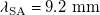
). Individual units are incrementally added, estimating the BL transition location following the addition of each element. Figure 7a illustrates that maximum transition delay is achieved for
$w_{\mathrm{SA}}={2}\,\mathrm{mm}$
). Individual units are incrementally added, estimating the BL transition location following the addition of each element. Figure 7a illustrates that maximum transition delay is achieved for $N_{\mathrm{SA}}=6$
, while
$N_{\mathrm{SA}}=6$
, while $N_{\mathrm{SA}}=5$
suffices to exhibit notable transition delay authority. Further addition of units yields limited effects on the BL transition location, suggesting the onset of a saturation effect.
$N_{\mathrm{SA}}=5$
suffices to exhibit notable transition delay authority. Further addition of units yields limited effects on the BL transition location, suggesting the onset of a saturation effect.
Variation of $x_{\mathrm{TR}}$
/c as a function of SA unit number, extracted from infrared (IR) images compared with the baseline configuration (
$x_{\mathrm{TR}}$
/c as a function of SA unit number, extracted from infrared (IR) images compared with the baseline configuration (![]() ): (a)
): (a) $k_{\mathrm{SA}}={0.07}{\,\mathrm{mm}}$
; (b)
$k_{\mathrm{SA}}={0.07}{\,\mathrm{mm}}$
; (b) $k_{\mathrm{{SA}}}={0.14}{\,\mathrm{mm}}$
.
$k_{\mathrm{{SA}}}={0.14}{\,\mathrm{mm}}$
.

Similar behaviour is observed when doubling the SA amplitude and increasing the number of units $(k_{\mathrm{{SA}}}={0.14}{\,\mathrm{mm}}, N_{\mathrm{SA}}=20)$
, as can be seen in Figure 7b. With these taller elements, cumulative transition delay is achieved up to
$(k_{\mathrm{{SA}}}={0.14}{\,\mathrm{mm}}, N_{\mathrm{SA}}=20)$
, as can be seen in Figure 7b. With these taller elements, cumulative transition delay is achieved up to $N_{\mathrm{SA}}=11$
, possibly due to a more favourable relationship between BL thickness and
$N_{\mathrm{SA}}=11$
, possibly due to a more favourable relationship between BL thickness and $k_{\mathrm{{SA}}}$
at downstream chord locations. Nevertheless, significant control capability is evident even when
$k_{\mathrm{{SA}}}$
at downstream chord locations. Nevertheless, significant control capability is evident even when $N_{\mathrm{SA}}=5$
, while
$N_{\mathrm{SA}}=5$
, while $N_{\mathrm{SA}}\geq 11$
results in a reduction to the achieved transition delay before reaching saturation. This behaviour is indicative of the presence of competing flow mechanisms governing the interaction between the BL and the SA, the identification of which is the subject of ongoing investigations.
$N_{\mathrm{SA}}\geq 11$
results in a reduction to the achieved transition delay before reaching saturation. This behaviour is indicative of the presence of competing flow mechanisms governing the interaction between the BL and the SA, the identification of which is the subject of ongoing investigations.
The influence of the parameters of SA amplitude $(k_{\mathrm{SA}})$
, chord location
$(k_{\mathrm{SA}})$
, chord location $(x_{\mathrm{SA}}/c)$
and width
$(x_{\mathrm{SA}}/c)$
and width $(w_{\mathrm{SA}})$
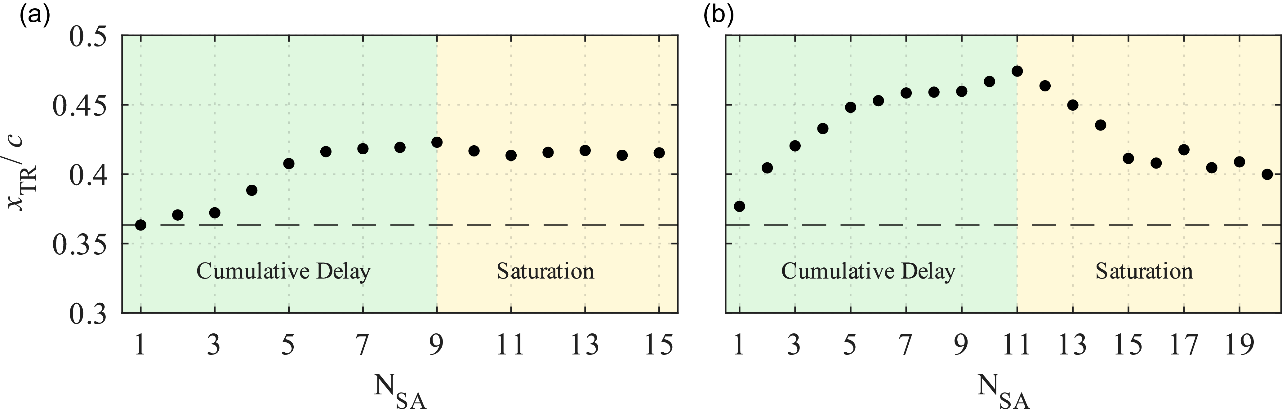
on the transition location is shown in Figure 8. As seen in Figure 8a, all forcing amplitude cases exhibit significant transition delay. Notably, an SA with elements of amplitude
$(w_{\mathrm{SA}})$
on the transition location is shown in Figure 8. As seen in Figure 8a, all forcing amplitude cases exhibit significant transition delay. Notably, an SA with elements of amplitude $k_{\mathrm{SA}}={0.14}{\,\mathrm{mm}}$
achieves laminar flow extension by nearly 10 % of the chord length. In turn, variation of the streamwise location of the first SA unit
$k_{\mathrm{SA}}={0.14}{\,\mathrm{mm}}$
achieves laminar flow extension by nearly 10 % of the chord length. In turn, variation of the streamwise location of the first SA unit $(x_{\mathrm{SA}}/c)$
is examined for an SA height of
$(x_{\mathrm{SA}}/c)$
is examined for an SA height of $k_{\mathrm{SA}}={0.07}{\,\mathrm{mm}}$
to avoid the possibility of inducing flow tripping at upstream chord locations. The resulting transition locations are illustrated in Figure 8
b and indicate that the reference chord-wise location,
$k_{\mathrm{SA}}={0.07}{\,\mathrm{mm}}$
to avoid the possibility of inducing flow tripping at upstream chord locations. The resulting transition locations are illustrated in Figure 8
b and indicate that the reference chord-wise location, $x_{\mathrm{SA}}/c=0.125$
, appears optimal, while both upstream and downstream shifts of the control configuration are detrimental to the control authority. Finally, as seen in Figure 8c, variation of each unit’s width indicates that
$x_{\mathrm{SA}}/c=0.125$
, appears optimal, while both upstream and downstream shifts of the control configuration are detrimental to the control authority. Finally, as seen in Figure 8c, variation of each unit’s width indicates that $w_{\mathrm{SA}}={2}{\,\mathrm{mm}}$
(comparable to the diameter of the DRE elements) provides the most significant transition delay.
$w_{\mathrm{SA}}={2}{\,\mathrm{mm}}$
(comparable to the diameter of the DRE elements) provides the most significant transition delay.
Transition location, $x_{\mathrm{TR}}$
, extracted from IR images for the combination of the baseline configuration (A8,
$x_{\mathrm{TR}}$
, extracted from IR images for the combination of the baseline configuration (A8, ![]() ) with a control configuration comprising an SA with 5 units of varying: (a) amplitude; (b) chord location of the first unit; and (c) width.
) with a control configuration comprising an SA with 5 units of varying: (a) amplitude; (b) chord location of the first unit; and (c) width.

For a roughness configuration composed of critical DREs and SAs, the maximum transition delay is obtained at $k_{\mathrm{SA}}={0.14}{\,\mathrm{mm}}$
. This value is therefore adopted as the baseline SA geometry for a width of
$k_{\mathrm{SA}}={0.14}{\,\mathrm{mm}}$
. This value is therefore adopted as the baseline SA geometry for a width of $w_{\mathrm{SA}}={2}\,\mathrm{mm}$
. Moreover, given that numerous forcing and control configurations are examined, it is advantageous to use a limited number of units to facilitate both application and removal. Consequently, SAs consisting of five units
$w_{\mathrm{SA}}={2}\,\mathrm{mm}$
. Moreover, given that numerous forcing and control configurations are examined, it is advantageous to use a limited number of units to facilitate both application and removal. Consequently, SAs consisting of five units $(N_{\mathrm{SA}}=5)$
are employed; the array starting at
$(N_{\mathrm{SA}}=5)$
are employed; the array starting at $x_{\mathrm{SA}}/c=0.125$
. These geometrical characteristics are retained throughout the remainder of this study. Note that preliminary investigations at a range of Reynolds numbers
$x_{\mathrm{SA}}/c=0.125$
. These geometrical characteristics are retained throughout the remainder of this study. Note that preliminary investigations at a range of Reynolds numbers $(1.8 \times 10^6 {-} 2.6\times 10^6)$
led to the same conclusions, with the difference that the the strip array wavelength was scaled to the respective critical wavelength. Consequently, this report focusses on a single Reynolds number
$(1.8 \times 10^6 {-} 2.6\times 10^6)$
led to the same conclusions, with the difference that the the strip array wavelength was scaled to the respective critical wavelength. Consequently, this report focusses on a single Reynolds number $(2.17\times 10^6)$
.
$(2.17\times 10^6)$
.
4. Influence of SA periodicity under different roughness configurations
As mentioned earlier, due to the highly polished surface of the M3J wing and low free-stream turbulence intensity of the LTT facility, BL-forcing via DRE or DRP configurations is necessary for achieving laminar–turbulent transition upstream of the wing’s pressure minimum. Independent of forcing configuration, the measured IR field as well as the PIV flowfields confirm that transition is dominated by growth and breakdown of stationary CFI. The results presented in this section cover a wide variety of forcing and control configurations; therefore, it is worth clarifying that within this work, a forcing configuration is composed by a single DRE array or DRP, and provides the baseline BL flow and transition location $(x_{\mathrm{TR, b}})$
. The control configuration is obtained by adding an SA with specific
$(x_{\mathrm{TR, b}})$
. The control configuration is obtained by adding an SA with specific $\lambda _{\mathrm{SA}}$
, resulting in the controlled transition location
$\lambda _{\mathrm{SA}}$
, resulting in the controlled transition location $(x_{\mathrm{TR}})$
. The transition front location and its modifications are discussed in a differential framework: namely, for each control case,
$(x_{\mathrm{TR}})$
. The transition front location and its modifications are discussed in a differential framework: namely, for each control case, $\Delta x_{\mathrm{TR}}/c$
is computed as
$\Delta x_{\mathrm{TR}}/c$
is computed as $(x_{\mathrm{TR}}-x_{\mathrm{TR, b}})/c$
. This framework is necessary because, given the extent of the parameter space, the DREs had to be replaced multiple times, requiring back-and-forth changes between DRE wavelengths. As a result, due to the proximity of the DREs to the leading edge, the exact positions of
$(x_{\mathrm{TR}}-x_{\mathrm{TR, b}})/c$
. This framework is necessary because, given the extent of the parameter space, the DREs had to be replaced multiple times, requiring back-and-forth changes between DRE wavelengths. As a result, due to the proximity of the DREs to the leading edge, the exact positions of $x_{\mathrm{TR, b}}$
for a given DRE wavelength was not identical across all cases, but varied within
$x_{\mathrm{TR, b}}$
for a given DRE wavelength was not identical across all cases, but varied within ${0.1}{}c$
. The average values are summarised in Table 1.
${0.1}{}c$
. The average values are summarised in Table 1.
4.1. DRE-forced boundary layer
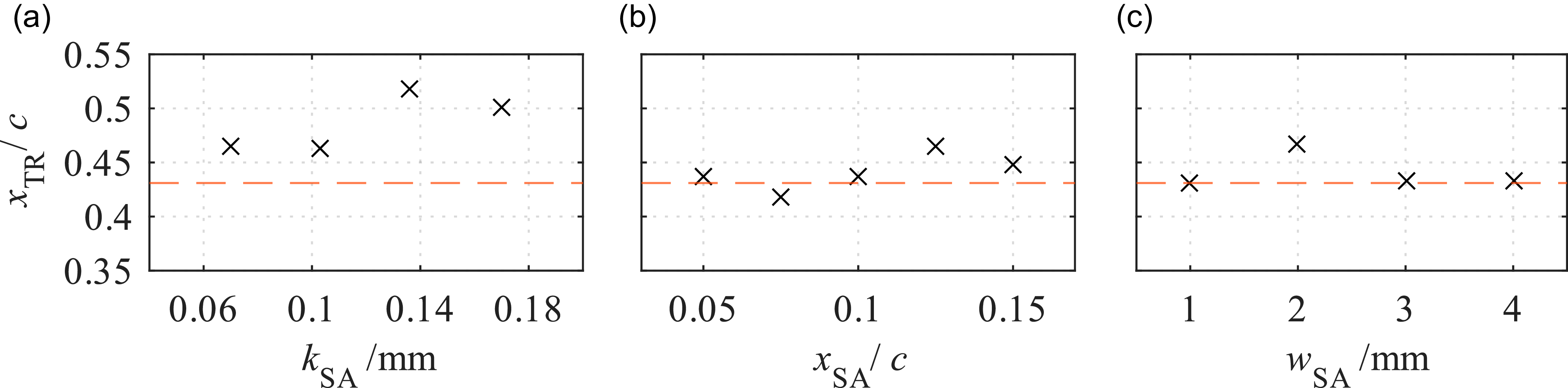
All SA configurations applied in a DRE-forced BL result in a significant delay of the transition location, as seen in Figure 9. When applied in a sub-critically forced BL (A6), SAs of any of the considered $\lambda _{\mathrm{SA}}$
are capable of delaying transition up to
$\lambda _{\mathrm{SA}}$
are capable of delaying transition up to $x/c\simeq 0.65$
, where the aerofoil pressure coefficient reaches its peak value (Serpieri Reference Serpieri2018). Due to the pressure gradient becoming adverse at this location, the BL transition in these cases cannot be attested to CFI breakdown, rather it is driven by laminar separation. Furthermore, for the considered
$x/c\simeq 0.65$
, where the aerofoil pressure coefficient reaches its peak value (Serpieri Reference Serpieri2018). Due to the pressure gradient becoming adverse at this location, the BL transition in these cases cannot be attested to CFI breakdown, rather it is driven by laminar separation. Furthermore, for the considered $Re_c$
, the forced sub-critical CFI mode (i.e. 6 mm) stabilises downstream of
$Re_c$
, the forced sub-critical CFI mode (i.e. 6 mm) stabilises downstream of $x/c \simeq 0.35$
(see Figure 2); therefore, damping this sub-critical CFI mode for a long enough portion of the wing chord is sufficient to prevent its growth to saturation and breakdown levels. At the same time, the forcing and initial growth of the sub-critical CFI mode inhibits the onset and development of critical modes (Saric et al. Reference Saric, Carrillo and Reibert1998; Wassermann & Kloker Reference Wassermann and Kloker2002).
$x/c \simeq 0.35$
(see Figure 2); therefore, damping this sub-critical CFI mode for a long enough portion of the wing chord is sufficient to prevent its growth to saturation and breakdown levels. At the same time, the forcing and initial growth of the sub-critical CFI mode inhibits the onset and development of critical modes (Saric et al. Reference Saric, Carrillo and Reibert1998; Wassermann & Kloker Reference Wassermann and Kloker2002). $\Delta x_{\mathrm{TR}}/c$
extracted from IR images for the combination of a baseline forcing configuration (A6, A7, A8 or A10) and a control configuration featuring SAs of various periodicities,
$\Delta x_{\mathrm{TR}}/c$
extracted from IR images for the combination of a baseline forcing configuration (A6, A7, A8 or A10) and a control configuration featuring SAs of various periodicities, $\lambda _{\mathrm{SA}}$
. Dashed lines correspond to a second-order polynomial fit.
$\lambda _{\mathrm{SA}}$
. Dashed lines correspond to a second-order polynomial fit.
Furthermore, Figure 9 shows that BLs forced by near-critical (A7), critical (A8) and super-critical (A10) DRE arrays are more sensitive to the SA periodicity, $\lambda _{\mathrm{SA}}$
, yet not all are as effective. More specifically, for near-critical forcing, overall reduced transition delay with respect to the sub-critical baseflow BL is observed, while for the critical and super-critical cases, the laminar flow region is extended by almost 10 % chord for an SA of optimal periodicity. All three forcing cases are more sensitive to the range of SA periodicity between 8 mm and 11.5 mm, comparing well to the range of streamwise wavelengths of the forced (and dominant) CFI modes
$\lambda _{\mathrm{SA}}$
, yet not all are as effective. More specifically, for near-critical forcing, overall reduced transition delay with respect to the sub-critical baseflow BL is observed, while for the critical and super-critical cases, the laminar flow region is extended by almost 10 % chord for an SA of optimal periodicity. All three forcing cases are more sensitive to the range of SA periodicity between 8 mm and 11.5 mm, comparing well to the range of streamwise wavelengths of the forced (and dominant) CFI modes $(\lambda _x={8.0}{\,\mathrm{mm}}$
, 9.2 mm and 11.5 mm, respectively
$(\lambda _x={8.0}{\,\mathrm{mm}}$
, 9.2 mm and 11.5 mm, respectively $)$
.
$)$
.
Although it does not fully describe the transitional behaviour, a simple least-squares quadratic fit adequately captures the main variations of $\Delta x_{\mathrm{TR}}/c$
induced by changes in
$\Delta x_{\mathrm{TR}}/c$
induced by changes in $\lambda _{\mathrm{SA}}$
(see Figure 9). From this fit, the periodicity of the maximum transition delay for each forcing configuration can be estimated by locating the apex of the curve. The resulting values of
$\lambda _{\mathrm{SA}}$
(see Figure 9). From this fit, the periodicity of the maximum transition delay for each forcing configuration can be estimated by locating the apex of the curve. The resulting values of $\lambda _{\mathrm{SA}}$
are 12.2, 14.5, 8.5 and 8.3 for A6, A7, A8, and A10, respectively.
$\lambda _{\mathrm{SA}}$
are 12.2, 14.5, 8.5 and 8.3 for A6, A7, A8, and A10, respectively.
4.2. DRP-forced and DRE/DRP-forced boundary layer
Considering the evident control capabilities demonstrated by SA arrays applied in DRE-forced BLs, their effectiveness is also investigated for BLs with increased background roughness. As mentioned earlier in this report, to enhance the roughness of the model surface, a distributed roughness patch (DRP) is applied at $x_{\mathrm{DRP}}/c=0.03$
to force the simultaneous development of multiple stationary CFI modes, resembling more realistic conditions. DRP forcing alone (without DREs) results in BL transition at
$x_{\mathrm{DRP}}/c=0.03$
to force the simultaneous development of multiple stationary CFI modes, resembling more realistic conditions. DRP forcing alone (without DREs) results in BL transition at $x/c\simeq 0.4$
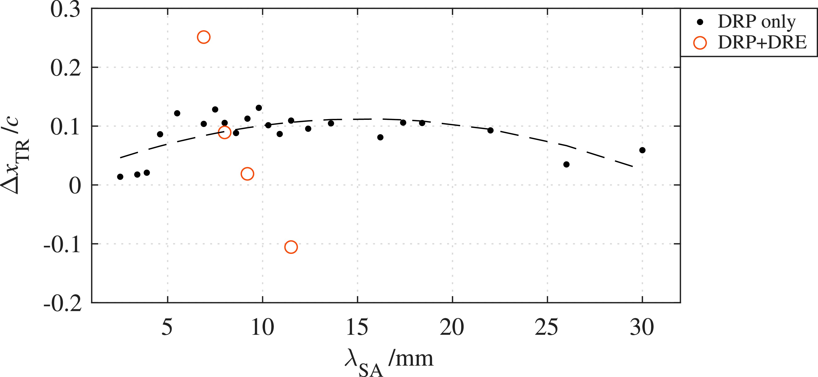
, while the transition location change obtained by adding SAs of various wavelengths is shown in Figure 10.
$x/c\simeq 0.4$
, while the transition location change obtained by adding SAs of various wavelengths is shown in Figure 10.
Owing to the loss of monochromatic periodicity in the BL, the $\Delta x_{\mathrm{TR}}/c$
achieved by the DRP and SA combination is more widespread than the respective observations in the previously discussed DRE-forced BL cases. Nonetheless, also in the presence of the DRP, a quadratic fit captures the overall behaviour of the controlled cases, with an apex at
$\Delta x_{\mathrm{TR}}/c$
achieved by the DRP and SA combination is more widespread than the respective observations in the previously discussed DRE-forced BL cases. Nonetheless, also in the presence of the DRP, a quadratic fit captures the overall behaviour of the controlled cases, with an apex at $\lambda _{\mathrm{SA}} = {15.3}{}$
. Yet, it is observed that for SAs with periodicity in the vicinity of 8 mm, transition delay is more effective, as wavelengths developing in the DRP case are expected to be at a wavelength range comparable to the critical one.
$\lambda _{\mathrm{SA}} = {15.3}{}$
. Yet, it is observed that for SAs with periodicity in the vicinity of 8 mm, transition delay is more effective, as wavelengths developing in the DRP case are expected to be at a wavelength range comparable to the critical one.
Building on this, the performance of critical-periodicity SAs in configurations combining simultaneous forcing with DRE arrays and DRP is also investigated. In these set-ups, the DRE array is placed upstream of the DRP at $x/c=0.02$
to impose a monochromatic CFI mode in the leading-edge region. The resulting BL flow is therefore expected to sustain a spectrum of small-wavelength CFI modes while concentrating most of the spectral energy on the forced mode (Zoppini et al. Reference Zoppini, Michelis, Ragni and Kotsonis2022
a). Subsequently, an SA with reference geometry and periodicity matching the wavelength of the forced mode is applied at
$x/c=0.02$
to impose a monochromatic CFI mode in the leading-edge region. The resulting BL flow is therefore expected to sustain a spectrum of small-wavelength CFI modes while concentrating most of the spectral energy on the forced mode (Zoppini et al. Reference Zoppini, Michelis, Ragni and Kotsonis2022
a). Subsequently, an SA with reference geometry and periodicity matching the wavelength of the forced mode is applied at $x/c=0.125$
. It should be noted that the baseline BL for these cases corresponds to the flow forced solely by the DRP, whereas the control configurations consist of the combined action of the DRE (A6, A7, A8 or A10) and the SA tuned to the corresponding critical wavelength.
$x/c=0.125$
. It should be noted that the baseline BL for these cases corresponds to the flow forced solely by the DRP, whereas the control configurations consist of the combined action of the DRE (A6, A7, A8 or A10) and the SA tuned to the corresponding critical wavelength.
The resulting transition locations are displayed in Figure 10 as red circular markers. These results, once more, demonstrate that a sub-critical DRE, when combined with the corresponding SA wavelength, $\lambda _{\mathrm{X}}$
, extends the laminar portion of the flow up to
$\lambda _{\mathrm{X}}$
, extends the laminar portion of the flow up to $x/c \simeq 0.65$
. This corresponds to
$x/c \simeq 0.65$
. This corresponds to $\Delta x_{\mathrm{TR}}/c \simeq 0.25$
, a particularly noteworthy outcome given that it is achieved in a flow scenario representative of real flight conditions. Further studies are required to assess the robustness of this result with respect to SA geometry, DRP location and flow conditions; nevertheless, this estimate strongly suggests that the proposed technique holds significant potential for in-flight applications.
$\Delta x_{\mathrm{TR}}/c \simeq 0.25$
, a particularly noteworthy outcome given that it is achieved in a flow scenario representative of real flight conditions. Further studies are required to assess the robustness of this result with respect to SA geometry, DRP location and flow conditions; nevertheless, this estimate strongly suggests that the proposed technique holds significant potential for in-flight applications.
Substantial transition delay is also achieved under near-critical DRE forcing, whereas in the critical BL, the control effectiveness is reduced compared with the case of DRP alone. This is consistent with the fact that, when the DRP is active, the growth of the critical CFI mode is partially suppressed by the simultaneous amplification of small-wavelength modes. Conversely, with A8 applied near the leading edge, the growth of the $\lambda _1$
mode is promoted; in combination with the broader spectral content induced by the DRP, this leads to rapidly amplifying instabilities that break down earlier. A similar effect occurs with A10, where a super-critical CFI mode is excited and evolves alongside the most critical
$\lambda _1$
mode is promoted; in combination with the broader spectral content induced by the DRP, this leads to rapidly amplifying instabilities that break down earlier. A similar effect occurs with A10, where a super-critical CFI mode is excited and evolves alongside the most critical $\lambda _1$
mode. This configuration is the only one to produce transition advancement, i.e. a reduction of the laminar region relative to DRP forcing alone.
$\lambda _1$
mode. This configuration is the only one to produce transition advancement, i.e. a reduction of the laminar region relative to DRP forcing alone. $\Delta x_{\mathrm{TR}}/c$
extracted from IR images for DRP forcing only featuring SAs of various periodicities,
$\Delta x_{\mathrm{TR}}/c$
extracted from IR images for DRP forcing only featuring SAs of various periodicities, $\lambda _{\mathrm{SA}}$
, and the corresponding second-order polynomial fit (
$\lambda _{\mathrm{SA}}$
, and the corresponding second-order polynomial fit (![]() ). For the DRP + DRE case, the SA wavelength corresponds to the wavelength of the DRE forced mode (A6, A7, A8 or A10).
). For the DRP + DRE case, the SA wavelength corresponds to the wavelength of the DRE forced mode (A6, A7, A8 or A10).

4.3. CFI amplitude as a function of SA periodicity
To validate the results provided by the IR investigation, for some of the considered roughness configurations, the local BL characteristics are estimated by analysing PIV measurements acquired at $x/c=0.3$
. Hereafter, the critical forcing case (A8) is considered in comparison to the flow field incurred by the application of the corresponding critical SA (A8,
$x/c=0.3$
. Hereafter, the critical forcing case (A8) is considered in comparison to the flow field incurred by the application of the corresponding critical SA (A8, $N_{\mathrm{SA}}=5$
,
$N_{\mathrm{SA}}=5$
, $\lambda _{\mathrm{SA}}={9.2}{\,\mathrm{mm}}$
). Figures 11a and 11c show the
$\lambda _{\mathrm{SA}}={9.2}{\,\mathrm{mm}}$
). Figures 11a and 11c show the $\overline {w}_d$
velocity field for the baseline and controlled cases, respectively. Considered in combination with Figure 11e showing the relevant BL and disturbance velocity profiles, it appears that only a mild reduction of the BL disturbance is obtained in the controlled cases. Nonetheless, the disturbance profiles
$\overline {w}_d$
velocity field for the baseline and controlled cases, respectively. Considered in combination with Figure 11e showing the relevant BL and disturbance velocity profiles, it appears that only a mild reduction of the BL disturbance is obtained in the controlled cases. Nonetheless, the disturbance profiles $\langle w \rangle _z$
show quantifiable CFI amplitude reduction, justifying the transition delay observed by IR imaging. In both the baseline and controlled cases, the
$\langle w \rangle _z$
show quantifiable CFI amplitude reduction, justifying the transition delay observed by IR imaging. In both the baseline and controlled cases, the $\langle w \rangle _z$
profile features a secondary peak indicative of the onset nonlinearities, which is reduced by applying the control SA.
$\langle w \rangle _z$
profile features a secondary peak indicative of the onset nonlinearities, which is reduced by applying the control SA.
(a) Mean velocity disturbance component, BL forced only critically (A8); (b) standard deviation, BL forced only critically (A8); (c) mean velocity disturbance component, BL forced critically (A8) and with an SA ( $N_{\mathrm{SA}}=5$
,
$N_{\mathrm{SA}}=5$
, $\lambda _{\mathrm{SA}}={9.2}{\,\mathrm{mm}}$
); (d) standard deviation, BL forced critically (A8) and with an SA (
$\lambda _{\mathrm{SA}}={9.2}{\,\mathrm{mm}}$
); (d) standard deviation, BL forced critically (A8) and with an SA ( $N_{\mathrm{SA}}=5$
,
$N_{\mathrm{SA}}=5$
, $\lambda _{\mathrm{SA}}={9.2}\,{\,\mathrm{mm}}$
); (e) mean BL profile,
$\lambda _{\mathrm{SA}}={9.2}\,{\,\mathrm{mm}}$
); (e) mean BL profile, $\overline {w}_b$
, standard deviations along the
$\overline {w}_b$
, standard deviations along the $z$
directions of mean velocity,
$z$
directions of mean velocity, $\langle \overline {w} \rangle _z$
, and of velocity standard deviation,
$\langle \overline {w} \rangle _z$
, and of velocity standard deviation, $\langle \sigma _w \rangle _z$
, as well as FFT amplitudes of the disturbance field. Solid lines correspond to forcing only with DRE A8, while dashed lines with DRE A8 and SA (
$\langle \sigma _w \rangle _z$
, as well as FFT amplitudes of the disturbance field. Solid lines correspond to forcing only with DRE A8, while dashed lines with DRE A8 and SA ( $N_{\mathrm{SA}}=5$
,
$N_{\mathrm{SA}}=5$
, $\lambda _{\mathrm{SA}}={9.2}\,{\,\mathrm{mm}}$
). Profiles are normalised with their maximum value.
$\lambda _{\mathrm{SA}}={9.2}\,{\,\mathrm{mm}}$
). Profiles are normalised with their maximum value.

The presence of the SA also influences the unsteady component of the instabilities, here quantified by the standard deviation of the velocity field, $\sigma _w$
, shown in Figures 11b and 11d. In the controlled BL, the overall standard deviation decreases, as evident from both the contours and the spanwise standard deviation profile,
$\sigma _w$
, shown in Figures 11b and 11d. In the controlled BL, the overall standard deviation decreases, as evident from both the contours and the spanwise standard deviation profile, $\langle w^\prime \rangle _z$
, in Figure 11c. Nevertheless, in both cases, significant velocity fluctuations persist near the wall, spatially associated with type-III instabilities arising from interactions between primary stationary and primary travelling waves (Bonfigli & Kloker Reference Bonfigli and Kloker2007; Malik et al. Reference Malik, Li, Choudari and Chang1999; Serpieri & Kotsonis Reference Serpieri and Kotsonis2016; Wassermann & Kloker Reference Wassermann and Kloker2002). In contrast, the regions of elevated standard deviation observed in the outboard and inboard downwelling vortex regions coincide with high-shear layers where type-I and II secondary instabilities typically form (Malik et al. Reference Malik, Li, Choudari and Chang1999; Wassermann & Kloker Reference Wassermann and Kloker2002). The application of the SA reduces
$\langle w^\prime \rangle _z$
, in Figure 11c. Nevertheless, in both cases, significant velocity fluctuations persist near the wall, spatially associated with type-III instabilities arising from interactions between primary stationary and primary travelling waves (Bonfigli & Kloker Reference Bonfigli and Kloker2007; Malik et al. Reference Malik, Li, Choudari and Chang1999; Serpieri & Kotsonis Reference Serpieri and Kotsonis2016; Wassermann & Kloker Reference Wassermann and Kloker2002). In contrast, the regions of elevated standard deviation observed in the outboard and inboard downwelling vortex regions coincide with high-shear layers where type-I and II secondary instabilities typically form (Malik et al. Reference Malik, Li, Choudari and Chang1999; Wassermann & Kloker Reference Wassermann and Kloker2002). The application of the SA reduces $\sigma _w$
in these regions, thereby delaying the onset and growth of secondary instabilities – an essential mechanism for achieving BL transition delay.
$\sigma _w$
in these regions, thereby delaying the onset and growth of secondary instabilities – an essential mechanism for achieving BL transition delay.
Spanwise FFT analysis of the $\overline {w}_d$
signal confirms that the dominant mode periodicity, along with its harmonics, is preserved in the presence of the SA (Figure 12a). This enables isolation and tracking of the dominant
$\overline {w}_d$
signal confirms that the dominant mode periodicity, along with its harmonics, is preserved in the presence of the SA (Figure 12a). This enables isolation and tracking of the dominant $\lambda _1$
mode, represented by its FFT shape function (blue line in Figure 11e). The shape function closely follows the disturbance profile, but with slightly reduced amplitude, as it reflects only the dominant CFI mode, whereas
$\lambda _1$
mode, represented by its FFT shape function (blue line in Figure 11e). The shape function closely follows the disturbance profile, but with slightly reduced amplitude, as it reflects only the dominant CFI mode, whereas $\langle w \rangle _z$
includes contributions from all instabilities and disturbances in the BL. Furthermore, the zoomed-in subplot of the
$\langle w \rangle _z$
includes contributions from all instabilities and disturbances in the BL. Furthermore, the zoomed-in subplot of the $\lambda _1$
spectral peak shows that all controlled cases decrease its amplitude, with the strongest reduction obtained for an SA wavelength of
$\lambda _1$
spectral peak shows that all controlled cases decrease its amplitude, with the strongest reduction obtained for an SA wavelength of $\lambda _{\mathrm{SA}}={9.2}\,{\,\mathrm{mm}}$
, i.e. corresponding to
$\lambda _{\mathrm{SA}}={9.2}\,{\,\mathrm{mm}}$
, i.e. corresponding to $\lambda _{\mathrm{X}}$
for A8.
$\lambda _{\mathrm{X}}$
for A8.
(a) Spatial FFT spectra extracted at $y/\overline {\delta _w^*}={1}{}$
for the reference baseline case
$y/\overline {\delta _w^*}={1}{}$
for the reference baseline case $(\lambda _{\mathrm{SA}}=0)$
and selected controlled cases. (b) Amplitude reduction obtained in the controlled cases expressed as percentage difference with respect to the baseline case amplitude.
$(\lambda _{\mathrm{SA}}=0)$
and selected controlled cases. (b) Amplitude reduction obtained in the controlled cases expressed as percentage difference with respect to the baseline case amplitude.

By integrating the $\lambda _1$
mode shape function along
$\lambda _1$
mode shape function along $y$
, the corresponding CFI amplitude
$y$
, the corresponding CFI amplitude $(A_{\lambda _1})$
is computed, providing a quantitative estimate of the damping and delaying effect of the SA. This value is shown in Figure 12b as
$(A_{\lambda _1})$
is computed, providing a quantitative estimate of the damping and delaying effect of the SA. This value is shown in Figure 12b as $A_{\mathrm{diff}}$
, expressing the difference between the controlled and baseline reference amplitude as a percentage of the baseline case amplitude. In agreement with the previous discussions, the cases forced by
$A_{\mathrm{diff}}$
, expressing the difference between the controlled and baseline reference amplitude as a percentage of the baseline case amplitude. In agreement with the previous discussions, the cases forced by $\lambda _{\mathrm{SA}}$
in the range of 8 mm to 11.5 mm lead to an amplitude reduction of the order of 10 %–15 % of the baseline case amplitude (which for the A8 forcing reaches values of 0.11 %
$\lambda _{\mathrm{SA}}$
in the range of 8 mm to 11.5 mm lead to an amplitude reduction of the order of 10 %–15 % of the baseline case amplitude (which for the A8 forcing reaches values of 0.11 % $W_\infty$
). The amplitude reduction obtained for the other considered
$W_\infty$
). The amplitude reduction obtained for the other considered $\lambda _{\mathrm{SA}}$
is still significant, but reflects the lower transition delay observed for these cases (see Figure 9).
$\lambda _{\mathrm{SA}}$
is still significant, but reflects the lower transition delay observed for these cases (see Figure 9).
Comparable observations pertain to the sub-critical, near-critical and super-critical baseline and forced cases discussed in the previous section. For these cases, PIV acquisitions are only performed for the flow field controlled by the corresponding critical SA. In all of the considered configurations, the presence of the SA has been found to preserve the dominant flow periodicity while damping the amplitude of the dominant mode. The resulting $A_{\mathrm{diff}}$
values are reported as coloured circles in Figure 12b, still providing significant reduction of the developing CFI amplitudes.
$A_{\mathrm{diff}}$
values are reported as coloured circles in Figure 12b, still providing significant reduction of the developing CFI amplitudes.
5. Concluding remarks
This study investigates the efficacy of spanwise-invariant roughness strip arrays (SAs) for laminar flow control application in cross-flow-dominated BL. The control configuration is composed of a repetition of two-dimensional roughness elements in the form of spanwise strips with various periodicity along the wing chord. The control capabilities of the considered geometries are estimated monitoring the BL transition location and its variations through IR thermography. In addition, local PIV provides information of the BL spectral content and on the CFI amplitude variation for the measured controlled BL cases.
SAs are applied in a DRE-forced BL, in which the forced CFI mode dominates the BL development. As a first step, the optimal geometry (i.e. amplitude, width and chord-wise location) of the SA for the current application is found. For this optimal geometry, the sensitivity to streamwise wavelength is investigated for a range of sub-critical, critical and super-critical BLs. In sub-critically forced BL, low sensitivity to the SA wavelength is observed, as all the considered configurations provide 8 %–10 % transition delay. Stronger sensitivity to SA periodicity is observed for critical and super-critical BLs, with stronger transition delay provided by those SA with $\lambda _{\mathrm{X}}$
comparable to the dominant CFI mode.
$\lambda _{\mathrm{X}}$
comparable to the dominant CFI mode.
Such control capabilities are retained in the presence of enhanced distributed surface roughness, providing a scenario resembling the rough finishing of manufactured wing surfaces. Interestingly, in a DRP-forced BL, applying a control configuration that combines a DRE and an SA with corresponding critical streamwise wavelength provides transition delay when compared with the reference DRP-forced BL. This is particularly true for a sub-critically forced BL, where the combination with a corresponding critical $\lambda _x$
SA provides up to 30 % transition delay. An analysis of the CFI amplitude as a function of SA periodicity corroborates these findings, showing the controlled BL scenarios retain the dominant CFI mode wavelength providing a reduction in its amplitude.
$\lambda _x$
SA provides up to 30 % transition delay. An analysis of the CFI amplitude as a function of SA periodicity corroborates these findings, showing the controlled BL scenarios retain the dominant CFI mode wavelength providing a reduction in its amplitude.
In summary, this study outlines the potential of suitably designed spanwise-uniform periodic roughness configurations for laminar flow control applications, with implications extending to real-flight scenarios. The performance metrics of the control system were demonstrated to be highly sensitive to the parametric variations of SA geometry. Nevertheless, the study acknowledges the limitations associated with the available dataset, precluding a comprehensive understanding of the underlying flow mechanisms contributing to the observed transition delay. Consequently, future research endeavours will focus on conducting in-depth investigations to elucidate the governing flow mechanisms at play. In addition, the present configurations are idealised and do not represent a fully realistic operational environment. While real surfaces will inevitably contain localised defects (e.g. insect contamination or scratches), the present results suggest that the control mechanism itself is robust at the instability level, even if its practical realisation would require strategies to manage surface contamination.
Acknowledgements
We gratefully acknowledge Emiel Langedijk and Stefan Bernardy for their technical support.
Data availability statement
Raw data are available from the corresponding author.
Funding statement
The authors are grateful to the European Research Council for financially supporting this research through the GloWing Starting Grant (grant no. 803082).
Declaration of interests
The authors declare no conflict of interest.


 Open access