


Impact Statement
The flow asymmetry between the two halves of a cricket ball gives rise to several interesting aerodynamic phenomena. Using force data from experiments in a wind tunnel, the present study investigates the phenomena of conventional and reverse swing and the effectiveness of different seam angles in transitioning the flow. This characteristic flow asymmetry on a cricket ball is utilized to propose a type of delivery that can undergo a zigzag motion similar to that associated with a knuckleball pitch in baseball. Based on the final lateral deflection of the ball, the number of times the ball changes its direction of lateral movement in flight, and the reaction time available to the batter, we propose optimal release conditions to produce an effective knuckleball that can help the bowler deceive the batter.
1. Introduction
A knuckleball pitch, in baseball, is associated with an unpredictable trajectory that confuses the batter and is considered one of the hardest pitches to hit (Reference Borg and MorrisseyBorg & Morrissey, 2014). The ball is thrown to minimize its spin during flight. The original technique to realize a knuckleball is to release the ball using knuckles. Later, the grip was modified by certain players. For example, one may hold the ball with one's fingertips while using the thumb for balance. Irrespective of the grip used, the distinguishing characteristic of a knuckleball pitch is that it is released with a very low spin rate and undergoes seemingly random motion. An example of a knuckleball pitch of a baseball undergoing low spin is shown in figure 1.
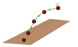
Seam orientation of the ball during its flight in a delivery referred to as knuckleball in cricket (red curve), the knuckleball pitch as used in baseball (blue curve) and the proposed model for a cricket knuckleball analogous to that used in baseball (green curve). The projection of the trajectories on the horizontal plane, shown in broken lines, reveals the lateral movement of the ball. We believe that the referral to the red curve as knuckleball in cricket is a misnomer; the correct interpretation is shown in the green curve. The letter ‘A’ is utilized as a marker to indicate the orientation of the ball.

Reference Watts and SawyerWatts and Sawyer (1975) offered an explanation for the erratic knuckleball trajectories seen in baseball. They proposed that the changing orientation of the seam on the baseball, with respect to the free-stream flow, results in a continuous shifting of the wake. Consequently, the lateral force also undergoes a continuous change in its direction causing the ball to undergo a zigzag motion. Such erratic trajectories have also been observed in soccer, particularly during the 2006 World Cup, when the ‘Teamgeist’ ball experienced the knuckleball phenomenon to a larger extent as compared with the balls used earlier (Reference Hong, Chung, Nakayama and AsaiHong, Chung, Nakayama, & Asai, 2010; Reference MehtaMehta, 2008).
Cricket is an outdoor bat-and-ball game played between two teams of eleven players each. A cricket ball consists of a cork interior encased by two leather hemispheres stitched together to form a prominent ‘seam’. This ball is propelled by a bowler towards the wicket defended by a batter. The aim of the bowler is to deceive the batter for which the bowler might attempt to move the ball laterally or vertically (Reference Deshpande, Shakya and MittalDeshpande, Shakya, & Mittal, 2018). ‘Spin bowlers’ deliver the ball at a relatively low speed and utilize the Magnus effect to create ‘drift’ and ‘dip’. Fast- and medium-paced bowlers ‘swing’ the ball for its lateral movement. The physics behind the ‘swing’ of a cricket ball has been studied extensively in the past (Reference BartonBarton, 1982; Reference Deshpande, Shakya and MittalDeshpande et al., 2018; Reference Shah, Shakya and MittalShah, Shakya, & Mittal, 2019). Reference MehtaMehta (1985) presented a comprehensive review on the subject.
The swing of a cricket ball is caused due to the asymmetry in flow on the two halves of the ball demarcated by a seam. This asymmetry can be created by (i) orienting the seam at an angle to the free stream (Reference Deshpande, Shakya and MittalDeshpande et al., 2018), (ii) differential surface roughness on the two halves of the ball (Reference Shah, Shakya and MittalShah et al., 2019), or (iii) providing a component of spin along the vertical axis to the ball (Reference MehtaMehta, 2014). When the ball moves laterally in the direction of the seam, the phenomenon is termed as conventional swing. Under certain conditions, the ball can also move in the direction opposite to the direction of the seam. This is known as reverse swing. Reference Scobie, Pickering, Almond and LockScobie, Pickering, Almond, and Lock (2013) presented experimental evidence for the formation of a separation bubble with late turbulent reattachment when the ball experiences reverse swing. In order to stabilize the orientation of the seam of the ball, the bowler usually imparts a backspin to the ball in the plane of the seam.
Knuckleball has attracted attention in cricket in recent times. Some deliveries from bowlers such as Bhuvneshwar Kumar and Andrew Tye have been referred to as knuckleball (Reference SarkarSarkar, 2018). At the outset, it should be noted that the terminology ‘knuckleball’ being used in cricket at this point in time is different than that used in baseball. The difference is on two counts. As opposed to baseball, many of the deliveries referred to as knuckleballs in cricket do not have the slow rotational speed associated with knuckleballs in baseball. The second difference is related to the axis of slow spin. Most cricket bowlers use the tip of their fingernails to deliver a knuckleball. Unlike regular swing bowling that is associated with backspin in the plane of the seam, this technique often lends a topspin to the ball with the plane of the seam itself rotating as shown with the red curve in figure 1. The flow, in this case, is symmetric about the  $x$–
$x$– $y$ plane passing through the centre of the ball. As a result, the ball does not experience any lateral force along the $z$ axis. Rather, the asymmetry of the flow with respect to the $x$–
$x$– $z$ plane causes the ball to experience a force in the $x$–
$x$– $y$ plane. However, this force is much smaller compared with gravity and, as a result, there is no zigzag motion even in the $x$–
$x$– $y$ plane associated with these trajectories. Indeed, the trajectory analysis of the deliveries in cricket that the commentators often describe as knuckleballs has revealed that they do not undergo the erratic direction-changing lateral movement as the knuckleball pitch used in baseball. Instead, such a delivery, with much lower speed, is used to deceive the batter with sudden variation of pace and increased dip due to the lack of backspin. The red curve in figure 1 shows the trajectory of a delivery that is commonly referred to as knuckleball in cricket. Its projection on the horizontal plane shows that, unlike the knuckleball pitch in baseball, this delivery does not exhibit the characteristic zigzag lateral movement. Therefore, we believe that it is not appropriate to refer to it as a knuckleball.
The objectives of the present study are (i) to investigate whether a cricket ball can experience a knuckleball phenomenon similar to that observed in baseball, and (ii) to find the optimal combinations of parameters that lead to an effective knuckleball that is difficult for the batter to play. To this end, it is proposed that the very slow spin imparted to the cricket ball be in the manner shown in the green curve in figure 1. Let  $N$ be the number of rotations that the seam undergoes during the flight of the ball. The illustration is for $N=0.5$. The axis of spin is closer to being vertical, rather than horizontal. It will be demonstrated later in the paper that the trajectory for such a delivery is associated with the zigzag motion similar to that for baseball. We carry out force measurement experiments on a cricket ball oriented at different seam angles and utilize the results to estimate the trajectory of the ball delivered at different speeds, orientations and rotation rates. The trajectories so obtained are analysed for their effectiveness in terms of the difficulty they might pose to the batter.
2. Experimental set-up
Force measurement experiments were conducted in a closed-circuit suction-type atmospheric wind tunnel. The test section has a rectangular cross-section of size  $3\,{\rm m} \times 2.25\,{\rm m}$. The maximum achievable speed in the test section is 80 m s $^{-1}$. The spatial inhomogeneity of the incoming flow was measured to be approximately 0.05 % at a speed of 20 m s $^{-1}$. The turbulence intensity is below 0.06 % for the entire operating speed range of the tunnel. Further details on the characterization of the wind tunnel can be found in the paper by Reference Cadot, Desai, Mittal, Saxena and ChandraCadot, Desai, Mittal, Saxena, and Chandra (2015).
Wind tunnel experiments were carried out on a new Sanspareils Greenlands (SG) Test cricket ball that is used in international Test matches played in India. The seam was orientated at angles ranging from  $0^{\circ }$ to $90^{\circ }$ to the incoming flow with an increment of $10^{\circ }$ per experiment. The wind speed was varied from 10 to 75 m s $^{-1}$ (36–270 km h $^{-1}$). The corresponding $Re$ range estimated on the basis of the diameter of the ball ( $=$71 mm) and kinematic viscosity of air at $25\,^{\circ }{\rm C}\ ({=}1.562 \times 10^{-5}\,{\rm m}^{2}\,{\rm s}^{-1})$ is $0.45 \times 10^5\unicode{x2013}3.40 \times 10^5$. The temperature in the test section of the wind tunnel was recorded in real time during the experiment. Its effect on the change of viscosity of air has been incorporated in estimating the $Re$, for each wind speed, while presenting the results. We note that the bowling speed in cricket is usually limited to 150 km h $^{-1}$ (Reference MehtaMehta, 2018) The data are presented for the entire range of $Re$ for completeness.
The cricket ball was mounted on a horizontal sting fixed to a rigid vertical support, which in turn was anchored to the floor of the test section. A hole of sufficient depth drilled through the centreline of the cricket ball was used to attach the ball to the sting. The blockage ratio of the cross-sectional area of the cricket ball to the area of the test section is approximately 0.06 %.
A six-component, strain gauge based, force sensor was used to measure unsteady forces on the cricket ball. The balance has a total of 24 strain gauges. Figure 2 shows a schematic of the balance, the location of strain gauges and their arrangement in the various Wheatstone bridges. The centre of the balance is located at the centre of the drag measurement section. The strain gauges numbered 17 to 20, shown in the two sectional views of the drag section, are used to measure the drag force. The bending due to the normal force results in compressive and tensile strains on the strain gauges numbered 9 to 16 located in the forward and backward sections. These are used to measure the normal force as well as the pitching moment. The side force and the yawing moment are measured using the strain gauges numbered 1 to 8, while the gauges 21 to 24 are utilized to measure the rolling moment. The balance is calibrated on a rig, prior to the conduct of experiments, to resolve the contribution of various forces and moments in other channels.
Schematic of the force balance showing placement of strain gauges and their arrangement to form the Wheatstone bridge. (a) Sectional, (b) top and (c) side views of the balance. The strain gauges are numbered from 1 through 24. Their location, in each view, is marked with an ‘ $x$’. The gauges that are pasted on a face opposite to the side shown in the figure are circled. For example, gauges 1 and 2 are at the same axial location, but 2 is located on the face on the opposite side shown in (c). The arrangement of various strain gauges in the Wheatstone bridge is shown in (d). The direction of flow is from left to right.

The calibration curve of the sensor is linear. The head of the sensor was connected to the downstream end of the horizontal sting. The set-up is shown in figure 3. Also shown is the coordinate system used to describe the results. The flow is along the  $x$ axis that is also the direction of the drag. The force referred to as lateral ‘swing’ force in the paper is along the $z$ axis. In order to correct the force contributions due to the support sting, force measurements were carried out on the support sting alone, while the model was held in position by an alternate support. The experimental set-up as well as the technique for correction is similar to that used by Reference Suryanarayana, Pauer and MeierSuryanarayana, Pauer, and Meier (1993). At least 60 s of data was acquired from the balance at a sampling rate of 500 Hz for each $Re$ and amplified for higher accuracy. Reference Norman and McKeonNorman and McKeon (2011) recommended that the time averaging be carried out for a minimum of 2000 time units, based on a non-dimensional time $tU_{\infty }/D$, where $U_{\infty }$ and $D$ are the free-stream speed of the flow and the diameter of the ball, respectively. The non-dimensional time, for the present acquisition, is 5000 at the lowest flow speed that is well above the recommended value. The force measurements were repeated at least twice, at each $Re$. The results from the various runs are in excellent agreement. The data are collected in the ‘decreasing $Re$’ mode of operating the tunnel. The tunnel is first operated at the highest speed of interest for a certain seam configuration. After the data are acquired for that speed, the speed is lowered to the next value of interest and the flow is allowed to stabilize. More details on the experimental set-up can be found in our earlier work (Reference Deshpande, Kanti, Desai and MittalDeshpande, Kanti, Desai, & Mittal, 2017).
Experimental set-up for the force measurement experiments on an SG Test ball.

3. Results and discussion
3.1 Aerodynamic analysis
Force measurements were carried out for seam angles ( $\phi _{T}$) between $0^{\circ }$ and $90^{\circ }$ in intervals of $10^{\circ }$ and various $Re$. Let $C_{D}$ and $C_{Z}$ be the coefficients associated with drag and lateral forces, respectively, non-dimensionalized with the dynamic pressure and cross-sectional area of the ball. Also marked in the plots is the speed, $U$, corresponding to each $Re$ for ambient conditions of $25\,^{\circ } {\rm C}$ and 1 atm pressure. Figure 4 shows the variation of time averaged $C_D$ and $C_Z$ with $Re$ for different seam angles. For seam angles ranging from $0^{\circ }$ to $70^{\circ }$, the ball experiences three regimes with increase in $Re$: subcritical, critical and supercritical. These have been described in detail by Reference Chopra and MittalChopra and Mittal (2017) and Reference Deshpande, Kanti, Desai and MittalDeshpande et al. (2017) for flow past a smooth cylinder and sphere, respectively. They utilized the variation of drag force with $Re$ to classify the flow. We follow the same methodology in this work. The drag force on the ball is maximum at critical $Re$ and minimum at the onset of the supercritical regime (Reference AchenbachAchenbach, 1972). The critical $Re$ for various seam angles is marked in figure 5.
Variation of (a)  $C_{D}$ and (b) $C_{Z}$ with $Re$ for a new SG Test cricket ball with its seam oriented at different angles to the flow ( $\phi _{T}$).

Variation of force coefficients with seam angle  $\phi _{T}$ and Reynolds number $Re$. The critical $Re$ for each seam angle is marked with a solid diamond-shaped symbol in the left panel. Here the $\phi _{T}$, $Re$,
$Re$,  $C_{D}$ and $C_{Z}$ during a typical trajectory of the ball released with an initial speed of $U_{o} = 90$ km h $^{-1}$, seam angle of $\phi _{o} = 30^{\circ }$ and that undergoes one rotation during its flight ( $N = 1$), are marked with a black line. The upper case letters mark the ( $Re$,
$Re$,  $\phi _{T}$) state of the ball at various time instants during its flight shown in figure 6. Here $\phi _{T}$, shown in figure 6, is suitably transformed so that it lies between $0^{\circ }$ and $90^{\circ }$ in this figure. The broken lines, in the figure on the right, indicate the part of the trajectory where the lateral force is in the direction opposite to that indicated.

At high subcritical  $Re$,
$Re$,  $C_D$ is in the range 0.4 to 0.48 for seam angles between $0^{\circ }$ to $70^{\circ }$. It is less than the corresponding $C_D$ for a smooth sphere ( $=$0.5). The subcritical $C_D$ is also found to decrease with increasing seam angle. It is highest in the case of a $0^{\circ }$ seam angle and lowest in the case of a $70^{\circ }$ seam angle. The curves corresponding to $80^{\circ }$ and $90^{\circ }$ seam angles indicate that the flow is already in the critical regime for the lowest $Re$ for which the experiment is conducted. In general, the transition to turbulence occurs at a lower $Re$ with increasing seam angle. This is evident from figure 4 that shows the preponement of drag crisis to lower $Re$ as the seam angle is increased from $0^{\circ }$ to $90^{\circ }$.
For a fixed seam angle,  $C_D$ stays relatively constant with increasing $Re$ throughout the supercritical regime. This behaviour is similar to that of a sphere with an axisymmetric trip wire placed on its surface (Reference Son, Choi, Jeon and ChoiSon, Choi, Jeon, & Choi, 2011). However, unlike for the axisymmetrically placed surface trip wire that results in similar $C_{D}$ for various angles, the supercritical $C_D$ for the cricket ball is not the same for different seam angles. We note that each polar section of the ball encounters a different azimuthal angle of seam orientation. Furthermore, the supercritical $C_D$ for all seam angles is significantly greater than the supercritical $C_D$ for the surface trip wire ( $C_D=0.18$).
The flow on the seam and non-seam side are relatively unaffected by the seam, below a certain  $Re$ (Reference Deshpande, Shakya and MittalDeshpande et al., 2018). Therefore, the ball does not experience any significant lateral force. However, the seam affects the flow significantly beyond a certain $Re$ leading to a side force on the ball. The threshold $Re$ depends on the seam angle. The side force changes direction at a critical $Re$. For example, for $\phi _T = 30^{\circ }$ (see figures 4 and 5), the ball first experiences a seam side force towards the positive $z$ axis (see figure 3 for convention) for $Re<1.7\times 10^{5}$, and thereafter, a force towards the non-seam side (negative $z$ axis) for larger $Re$. As shown by Reference Deshpande, Shakya and MittalDeshpande et al. (2018) and Reference Shah, Shakya and MittalShah et al. (2019) for $\phi _T = 30^{\circ }$, for $Re$ less than the critical value, the flow undergoes transition on the seam side that delays flow separation on this half of the ball leading to increased suction. The flow on the non-seam side, however, stays laminar. The pressure differential created on the two halves of the ball due to this asymmetric flow transition leads to conventional swing. The side force coefficient increases with $Re$ and then stays nearly constant with a further increase in $Re$ in the regime of conventional swing. The variation of $C_{Z}$ with $Re$ is qualitatively similar for various seam angles barring a few differences. For example, $C_{Z}$ exhibits a ‘double-drop’ behaviour for $\phi _{T} = 10^{\circ }$, $20^{\circ }$ and $70^{\circ }$ where its decrease with an increase in $Re$ occurs in two stages during transition from conventional to reverse swing. We offer a possible explanation. The entire width of the seam lies on one side of the stagnation point, on the upstream face of the ball, for $\phi _{T} > 20^{\circ }$. However, this is not the case for $\phi _{T} \le 20^{\circ }$. Therefore, the seam affects the transition of the boundary layer on both halves of the ball leading to a relatively gradual drop in $C_{D}$ and $C_{Z}$ compared with that for larger seam angles. Reference Scobie, Shelley, Jackson, Hughes and LockScobie, Shelley, Jackson, Hughes, and Lock (2020) also observed similar behaviour for $\phi _{T} = 15^{\circ }$ albeit for an old ball. Reference Smith and SmithSmith and Smith (2021), from particle image velocimetry experiments on a non-spinning baseball in a wind tunnel, found that the seam orientation can alter the boundary layer separation on the two halves of the ball leading to asymmetry in the flow. They referred to the resulting flow downstream of the ball as a ‘seam shifted wake’. It was found that for a ball pitched at 90 mi h $^{-1}$ ( $=$144 km h $^{-1}$), the flow separates between $108^{\circ }$ and $120^{\circ }$ when there is no interference with the seam. However, the flow separates at the seam if it is located between $84^{\circ }$ and $108^{\circ }$. We utilize their observation to speculate the effect of seam orientation on the flow past a cricket ball. For $\phi _T = 70^{\circ }$ and $80^{\circ }$, the flow encounters the trip at $110^{\circ }$ and $100^{\circ }$, respectively, on the non-seam side. Therefore, it is possible that for moderate $Re$, as observed for baseball, the boundary layer on the non-seam side of the cricket ball undergoes separation at these angles without the formation of a laminar separation bubble, thereby causing a relatively gradual change from conventional to reverse swing. With a further increase in $Re$, the boundary layer transitions to a turbulent state, thereby delaying the separation of flow. The $Re$, at which $C_{Z}$ saturates, decreases with an increase in $\phi _{T}$. Also, the rate of increase of $C_{Z}$ with $Re$, prior to achieving the saturated value, increases with an increase in $\phi _{T}$. Both these observations point to an increase in the effectiveness of the seam, in transitioning the flow, with an increase in $\phi _{T}$.
For  $Re$ exceeding the critical value, the flow on the seam side goes into a supercritical state while the flow on the non-seam side undergoes a transition to a turbulent state. For example, for $\phi _T = 30^{\circ }$, the ball experiences a force opposite to the seam side for $Re>1.8 \times 10^{5}$. The seam thickens the turbulent boundary layer on the seam side resulting in an earlier flow separation compared with that on the non-seam side. In addition, there is a formation of a separation bubble and late turbulent reattachment on the non-seam side as experimentally demonstrated by Reference Scobie, Pickering, Almond and LockScobie et al. (2013). Therefore, suction on the non-seam side is larger, thereby causing the ball to experience reverse swing. The transition from conventional swing to reverse swing is accompanied with a very significant reduction in $C_{D}$. The drop in $C_{D}$ with $Re$ is relatively gradual for $\phi _{T} \le 20^{\circ }$ and very steep for higher seam angles. We note that the ball experiences reverse swing at fairly low $Re$ when the seam angle is $80^{\circ }$ or larger.
3.2 Trajectory of a knuckleball
The trajectory of the ball, delivered at a certain initial speed, rotation rate and seam orientation is estimated by integrating the following equation in time:  $m ({{\rm d} \boldsymbol {V}}/{{\rm d} t}) = \boldsymbol {F}$. Here, $m$ is the mass of the cricket ball, $\boldsymbol {V}$ its velocity and $\boldsymbol {F}$ the force acting on it. We restrict our attention to the motion of the ball in a horizontal plane. The lateral component of the velocity of the ball at the time of delivery is assumed to be zero. It is further assumed that the aerodynamic force acting on the ball at each time instant is the time-averaged force on the ball for the fully developed flow at the corresponding value of instantaneous $Re$ and seam orientation. The measurements from the wind tunnel testing of the SG Test cricket ball, shown in figure 4, are utilized to estimate $\boldsymbol {F}$ for ambient conditions corresponding to a $25\,^{\circ }{\rm C}$ temperature and 1 atm pressure. The mass of the ball is assumed to be the same as that of the standard SG Test cricket ball ( $=$0.156 kg). A time step of 0.001 s is utilized to integrate the equation of motion.
Since the force measurements were only carried out for seam angles from  $0^{\circ }$ to $90^{\circ }$ at increments of $10^{\circ }$, the $C_D$ and $C_Z$ values for intermediate angles are estimated via interpolation. Furthermore, the force coefficients for larger seam angles are determined using the symmetry of the cricket ball. The $C_D$ value for any angle $\phi _{T}$ ranging between $90^{\circ }$ to $180^{\circ }$ is the same as the $C_D$ value for the angle $180^{\circ } - \phi _{T}$ while the $C_Z$ value is the negative of the $C_Z$ value for the angle $180^{\circ } - \phi _{T}$. Owing to the symmetry of the ball, the $C_D$ and $C_Z$ values for an angle $\phi _{T}$ in the range of $180^{\circ }$ to $360^{\circ }$ are the same as those for the angle $\phi _{T} - 180^{\circ }$. Figure 5 shows the values of the force coefficients used for trajectory calculations. Although we have assumed symmetry, in reality, the two halves of the SG Test cricket ball have different surface markings that result in asymmetry in the flow. Furthermore, the balls may not be perfect spheres. We have assumed these effects are relatively small and the major asymmetry in the flow is caused by the orientation of the seam to the free-stream flow.
In order to bowl a baseball-style knuckleball in cricket, it is necessary for the ball to experience a lateral force that often changes direction leading to a zigzag, and seemingly random, motion during its flight. The easiest way to achieve this is to release the ball with a spin about the vertical axis as shown in figure 1. In addition, the spin imparted to the ball must be small enough so that the lateral force caused by the constantly changing asymmetric orientation of the seam dominates the fixed-direction Magnus force experienced by the ball. Based on the analysis of in-game pitches, Reference NathanNathan (2012) reported that the most effective knuckleballs are released with a spin that makes the ball undergo between 0.5–1.5 rotations on its way to the batter. Thus, we will restrict our analysis to deliveries that undergo a maximum of two rotations during their flight.
Based on the above discussion, we identify three variables that govern the motion of a knuckleball: initial speed ( $U(0)=U_{o}$), initial seam angle ( $\phi _{T}(0)=\phi _{o}$) and the number of rotations the ball undergoes in its flight ( $N$). The effect of gravity is ignored. Figure 6(a) shows one such trajectory for a cricket ball released with $U_{o} = 90\,{\rm km}\,{\rm h}^{-1}$, $N = 1$ and $\phi _o=30^{\circ }$. The lateral position of the ball, with respect to its initial location at delivery, as well as its seam orientation while it travels from one end of the pitch to the other, which is 20.12 m (22 yards) away, is shown in the figure. The ball slows down, due to air resistance, as it travels down the pitch leading to a decrease in its Reynolds number. Its seam orientation changes as well, due to spin. Here $C_{D}$ and $C_{Z}$, inferred from figure 5 for the local ( $Re$,
$Re$,  $\phi _{T}$) state, are shown in figure 6(b).
(a) Trajectory of a knuckleball released with  $U_{o} = 90\,{\rm km}\,{\rm h}^{-1}$, $\phi _{o} = 30^{\circ }$ and $N = 1$. Variation of $\phi _{T}$ as the ball moves along the pitch is also indicated. The stars indicate the points where the ball reverses the direction of its lateral movement, i.e. the lateral velocity is zero. The blue arrow is perpendicular to the seam of the ball and the black arrow indicates the direction of rotation. (b) Variation of force coefficients during the flight of the ball, estimated from the local $Re$ and seam orientation (see figure 5).

Point A in figure 6(a) shows the initial orientation of the ball as it travels towards the other end with a counterclockwise rotation as observed in the top view of the pitch. The ball experiences a large (conventional) swing force for this initial configuration of the seam (see figure 6b). Therefore, it undergoes a sharp lateral movement in the direction away from a right-handed batter. The lateral force acting on the ball changes direction as it moves down the pitch. For example, the seam angle  $\phi _{T}$ is $70^{\circ }$ at point B. The ball experiences reverse swing for this state of ( $Re$,
$Re$,  $\phi _{T}$), as can be observed from figure 6(b). The lateral force on the ball is along the negative $z$ axis causing it to decelerate while it continues to move laterally along the positive $z$ axis. At point D, about one-third of its way to the batter, the ball has slowed down considerably and experiences a near-constant negative side force. This causes the ball to change its direction of lateral movement for the first time in its flight. The event is identified with a blue star in figure 6(a). We note from the figure that, for these parameters, the ball changes its direction of lateral movement on four occasions.
Figure 7(a) shows the variation of the speed of the ball during its flight for various initial delivery speeds,  $U_{o}$, delivered at an initial seam angle of $\phi _{T} = 30^{\circ }$ with no spin as it reaches the other end of the pitch. Our calculations with other initial orientations of the seam ( $\phi _{o}$), not shown here, reveal that the variation of the speed of the ball during its flight along the pitch is roughly the same. The ball with an initial speed of 150 km h $^{-1}$ experiences a speed reduction of 9.9 %, while a ball with an initial speed of 60 km h $^{-1}$ experiences a speed reduction of 11.85 %. The percentage reduction in speed for other cases lies between these two values. These values are nearly identical to the speed reduction reported by Reference BakerBaker (2010) and Reference Deshpande, Shakya and MittalDeshpande et al. (2018).
Effect of initial speed ( $U_{o}$) on the trajectory of a ball released with zero spin ( $N=0$) at initial seam angle ( $\phi _{o}$) of $30^{\circ }$: (a) variation of the speed of the ball as it travels across the pitch, and (b) trajectory of the ball for different initial speeds.

Figure 7(b) shows the trajectories of a cricket ball released at different initial speeds with zero rotation. For speeds between 60–135 km h $^{-1}$, the ball undergoes conventional swing, i.e. its lateral movement is towards the seam side. The lateral deflection of the ball when it reaches the wickets at the end of the batter is between 0.9–1.2 m. For the case of 145 and 150 km h $^{-1}$, the initial lateral movement of the ball is in the direction opposite to that of the seam since it experiences reverse swing. As the ball slows down, it experiences conventional swing and undergoes a lateral movement in the direction of the seam. Thus, it is possible for the ball to experience a change of direction in its lateral movement, once in its flight, even with zero rotation if it is delivered at a speed in the regime of reverse swing. The trajectory of the ball for 145 km h $^{-1}$ is reminiscent of late swing.
The final deflection for the ball with an initial speed of 150 km h $^{-1}$ is the lowest among all the different initial speeds. This can be attributed to two factors. The first reason is that the ball reaches the other end of the pitch in very little time. The second reason is that initially, the ball moves away from the seam and then towards the seam, making the net lateral movement much smaller. As the initial speed is decreased from 150 km h $^{-1}$, the net deflection of the ball at the end of the pitch increases. This is seen up to a speed of 90 km h $^{-1}$. A further decrease in speed below 90 km h $^{-1}$ results in smaller deflections compared with $U_{o} =90\,{\rm km}\,{\rm h}^{-1}$.
Figure 8 shows the effect of adding a slow spin to the ball in order to achieve the knuckleball phenomenon. Here  $N$ is the number of rotations the ball undergoes during its flight. For a ball delivered at a certain speed, an increase in $N$ corresponds to an increased spin rate. Unlike in the case of no spin, the side force on the ball with spin changes direction during its flight resulting in a smaller final deflection. With an increase in the rate of spin of the ball, the tendency of the ball to change its lateral direction increases. The ball also undergoes progressively less deflection as $N$ is increased. From the point of view of a bowler, an effective knuckleball involves a relatively large number of lateral direction changes while still undergoing a large enough final deflection to deceive the batter. For $N<0.5$, the ball does not rotate enough for the side force to change direction. With an increase in $N$, although the final deflection of the ball reduces, there are changes in direction causing the movement of the ball to be erratic and making it increasingly unpredictable for the batter. For $N>1$, the number of times the ball changes its direction in its trajectory increases rapidly. However, the lateral movement of the ball is much smaller making it relatively easier for the batter to judge it. Figure 8 shows the trajectory of the ball delivered at four different delivery speeds ranging from 60 to 150 km h $^{-1}$. It is similar for $U = 60$, 90 and 120 km h $^{-1}$. However, the reverse swing at 150 km h $^{-1}$ results in a relatively small deflection of the ball in a direction opposite to the direction to which the seam is angled.
Effect of  $N$ (number of ball rotations during the flight of the ball from one end of the pitch to the other): knuckleball trajectories at $\phi _{o}=30^{\circ }$ for $U_{o}=$ (a) 60 km h $^{-1}$, (b) 90 km h $^{-1}$, (c) 120 km h $^{-1}$ and (d) 150 km h $^{-1}$.

Next, we study the effect of seam angle at the point of release of the ball. Here  $U_{o}$, the initial speed of the ball, is assumed to be 90 km h $^{-1}$. Figure 9 shows the effect of $\phi _{o}$ for two rotation rates: $N=0.5$ and $N=2$. For a given $N$, the final deflection of the ball as well as the number of times the ball reverses its path is found to be very sensitive to $\phi _{o}$. Since the ball moves from a negative seam angle to a positive one for the case of $\phi _{o}=-20^{\circ }$, it experiences negative side force in the initial part of its trajectory followed by a positive force later on. Consequently, it undergoes a relatively small final deflection. The case corresponding to $\phi _{o} = 0^{\circ }$ is associated with the maximum deflection since it experiences the least number of reversals in the direction of lateral force. We now compare the trajectories for $N$=0.5 and $N=2$. For the case of $N=0.5$, the ball undergoes a large final deflection. However, the change in direction of the lateral movement is observed only for certain $\phi _{o}$. On the other hand, a large number of direction changes are observed for all $\phi _{o}$ for $N=2$. However, owing to the rapidly changing path direction, the final deflection is small.
Effect of initial seam angle ( $\phi _o$): knuckleball trajectories at $U_{0}=90$ km h $^{-1}$ for (a) $N = 0.5$ and (b) $N = 2$.

We attempt to identify an effective combination of the bowling parameters ( $U_{o}$, $\phi _{o}$, $N$) that result in trajectories with a high final deflection as well as a relatively large number of direction changes. For simplicity, we restrict to $\phi _{o}=30^{\circ }$. Let $M$ be the number of direction changes with respect to the lateral movement of the ball during its entire flight. Figure 10 shows the variation of final deflection ( $Z_{22}$) and the number of direction changes ( $M$) for different combinations of $U_{o}$ and $N$. We observe from the figure that, for low rotation rates ( $N\le 0.25$), the final deflection is high but the ball does not undergo direction changes for $U_{o}$ less than approximately 140 km h $^{-1}$. The lateral direction changes, for these low values of $N$, are observed only when $U_{o}$ is high and the ball enters both reverse swing and conventional swing regimes in its flight. Therefore, for an effective knuckleball with a very small rotation, the initial speed needs to be high. This might not be very practical as it is difficult for the bowler to release a high-speed delivery with a knuckleball grip.
Variation of the final deflection of the ball with  $U_{o}$ for different $N$ at $\phi _{o} = 30^{\circ }$. The thickness of the line represents the number of direction changes ( $M$) it undergoes in its flight. Here $M$ corresponding to some of the cases are marked on the figure. The optimal knuckleball associated with large $M$, significant lateral movement ( $Z_{22}$ close to 0.2 m) and a relatively large speed to provide less reaction time to the batter is marked in orange.

Here  $N\ge 1$ does not result in effective knuckleballs either. For example, figure 10 shows that the final deflection for the ball is small for all initial speeds for $N=1$ despite the number of direction changes being high. The $N=2$ case results in an almost identical curve (not shown in this figure). The case of $N=0.5$ is interesting. It can be seen from figure 10 that the ball undergoes a change of lateral direction for approximately $U_{o}\le 140$ km h $^{-1}$. In addition, the final deflection of the ball is significantly high for $U_{o}\le 115$ km h $^{-1}$. Thus, a delivery with $N=0.5$ and $U_{o}\le 115$ km h $^{-1}$ leads to a significant final deflection of approximately 0.2 m of the ball in addition to undergoing a change in the lateral direction. Reference JonesJones (2021) analysed the swing data for a red Kookaburra ball in different ambient and ball conditions from Test matches played in Australia over a period of five years. The average swing was found to be $0.69^{\circ }$ that translates to a 0.24 m lateral deflection of the ball over the length of the pitch. A knuckleball with a change of lateral direction and a final deflection of similar order can be expected to be challenging to the batter. Reference NathanNathan (2012) presented an analysis of knuckleball trajectories in baseball for two pitchers. The scatter plot for various pitches shows that the lateral deflection decreases with an increase in speed. The maximum deflection is of the order of 0.5 m for a release speed of approximately 115 km ${\rm h}^{-1}$. Since $Z_{22}$ and $M$ are nearly constant in this range, the optimal conditions for the knuckleball are at higher speeds in this range as they provide the least reaction time to the batter. This optimal region for a knuckleball is encircled in orange in figure 10.
4. Conclusions
We have proposed that imparting a small spin to a cricket ball about the vertical axis causes it to move along a zigzag path like the knuckleball pitch in baseball. The trajectory of such a delivery has been estimated using force data from wind tunnel experiments performed on a cricket ball in various seam orientations and flow speeds. We note that a ball delivered with spin about the horizontal axis cannot undergo similar direction changes in its lateral motion.
The experiments reveal that in the  $Re$ range of the study, the cricket ball experiences subcritical, critical and supercritical regimes for seam angles less than $70^{\circ }$. This affects the rate at which the ball slows down in its flight as there is a sharp increase in $C_{D}$ in the subcritical regime. With an increase in the seam angle of the ball, the critical $Re$ reduces. The drop in $C_{D}$ in the critical regime is steeper for higher seam angles. The flow is found to be already in the critical regime for seam angles greater than $70^{\circ }$. Here $C_{D}$ in the supercritical regime remains relatively constant with change in $Re$.
$Re$.
Beyond a certain  $Re$, the cricket ball experiences a lateral ‘swing’ force due to the flow asymmetry caused by an angled seam. For a fixed seam angle, the force coefficient $C_{Z}$ increases with an increase in $Re$ and then saturates. The effectiveness of the seam in transitioning the flow increases with an increase in $\phi _{T}$; $C_{Z}$ saturates to its maximum value at lower $Re$ with increasing $\phi _{T}$. For a fixed $\phi _{T}$, $C_{Z}$ suffers a steep drop to a negative value beyond a certain $Re$. This is referred to as ’reverse swing’ as this lateral force causes the ball to move away from the direction of the seam. For seam angles greater than $80^{\circ }$, this reversal occurs at fairly low $Re$. A ball with no spin ( $N=0$) experiences conventional swing and undergoes lateral deflection towards the seam side for $U_{o} \le 135$ km h $^{-1}$ without any direction change. For 142 km h $^{-1}\le U_{o} \le 150$ km h $^{-1}$, it exhibits one change in direction as the ball moves from the regime of reverse to conventional swing during its flight. A clever bowler can choose an appropriate $U_{o}$ to challenge the batter. While the maximum lateral deflection of the ball occurs for $U_{o}=105$ km h $^{-1}$, a ball delivered at a higher speed offers a lower reaction time to the batter.
The change in the direction of lateral force can also be achieved by a change in the seam orientation of the ball. For example, the seam angle, in a knuckleball with slow spin, changes continually resulting in changes in the direction of the lateral force acting on it. These direction changes give rise to the zigzag motion of the ball and are perceived as an erratic trajectory by the batter.
The motion of a knuckleball is governed by three variables:  $U_{o}$, $\phi _{0}$ and $N$. Unlike for a ball with no spin, a ball with spin can change its lateral direction even at low speeds as the swing force on it is constantly changing its direction. With an increase in $N$, the ball undergoes an increased number of direction changes in its lateral path. We refer to the number of these direction changes as $M$. It is found that the final deflection of the ball decreases as $M$ increases. The $N<0.5$ case does not generally cause direction changes but it is associated with a reasonably large final lateral deflection. The $N\ge 1$ case leads to an increase in $M$ but the final deflection is small. We propose that a ball with reasonably large $M$ and final deflection constitutes a difficult ball for the batter to play. Based on this analysis, the optimal speed and spin for an effective knuckleball are estimated to be $U_{o}=115\,{\rm km}\,{\rm h}^{-1}$ and $N=0.5$ approximately.
Funding statement
This research received no specific grant from any funding agency, commercial or not-for-profit sectors.
Declaration of interests
The authors declare no conflict of interest.
Data availability statement
The data presented in this study are available from the corresponding author upon reasonable request.


 Open access