





1 Introduction
Let
$(M,\omega ,{ \mathcal J})$
 be a compact connected symplectic manifold equipped with a Hamiltonian action of a compact connected Lie group G with moment map
${ \mathcal J}:M \rightarrow \mathbf {\mathfrak g}^\ast $
be a compact connected symplectic manifold equipped with a Hamiltonian action of a compact connected Lie group G with moment map
${ \mathcal J}:M \rightarrow \mathbf {\mathfrak g}^\ast $
 . Then the associated Marsden-Weinstein reduced space, or simply the symplectic quotient, is given by

If
$0$
 is a regular value of the moment map, the symplectic quotient naturally inherits the structure of a symplectic orbifold
$({\mathscr M}_0,\omega _0)$
is a regular value of the moment map, the symplectic quotient naturally inherits the structure of a symplectic orbifold
$({\mathscr M}_0,\omega _0)$
 , but in general, by a classical result of Sjamaar and Lerman [Reference Sjamaar and Lerman35], it is only a stratified symplectic space, each smooth stratum being naturally equipped with a symplectic structure.
This paper is devoted to the computation of the invariant Riemann-Roch number of
$(M,\omega ,{ \mathcal J})$
 in terms of the geometry of the associated symplectic quotient (1.1). To introduce it, one has to impose the condition that the cohomology class
$[\omega ]\in H^2(M,{\mathbb Z})$
in terms of the geometry of the associated symplectic quotient (1.1). To introduce it, one has to impose the condition that the cohomology class
$[\omega ]\in H^2(M,{\mathbb Z})$
 is integral, in which case
$(M,\omega )$
is integral, in which case
$(M,\omega )$
 is called quantizable. This condition is equivalent to the existence of a Hermitian line bundle
$(L,h^L)$
is called quantizable. This condition is equivalent to the existence of a Hermitian line bundle
$(L,h^L)$
 over M equipped with a Hermitian connection
$\nabla ^L$
over M equipped with a Hermitian connection
$\nabla ^L$
 with curvature
$R^L$
with curvature
$R^L$
 satisfying the prequantization condition

The Hamiltonian G-manifold
$(M,\omega ,{ \mathcal J})$
 is prequantized if the action of G lifts to an action on
$(L,h^L,\nabla ^L)$
is prequantized if the action of G lifts to an action on
$(L,h^L,\nabla ^L)$
 and the moment map
${ \mathcal J}:M \rightarrow \mathbf {\mathfrak g}^\ast $
and the moment map
${ \mathcal J}:M \rightarrow \mathbf {\mathfrak g}^\ast $
 is given in terms of the lifted action by the Kostant formula (2.12). Upon choosing a G-invariant almost complex structure
$J\in \operatorname {\mathrm {End}}(TM)$
is given in terms of the lifted action by the Kostant formula (2.12). Upon choosing a G-invariant almost complex structure
$J\in \operatorname {\mathrm {End}}(TM)$
 over M compatible with
$\omega $
over M compatible with
$\omega $
 , one gets a Riemannian metric on M defined by

One can then consider the associated Spin
$^c$
 -Dirac operators
$D^\pm :\Omega ^{0,\pm }(M,L)\to \Omega ^{0,\mp }(M,L)$
-Dirac operators
$D^\pm :\Omega ^{0,\pm }(M,L)\to \Omega ^{0,\mp }(M,L)$
 defined in Section 2.2, which are elliptic first order differential operators, and thus have finite dimensional kernels. The action of G on
$(L,h^L)$
defined in Section 2.2, which are elliptic first order differential operators, and thus have finite dimensional kernels. The action of G on
$(L,h^L)$
 induces an action on these kernels, and one defines the associated invariant Riemann-Roch number as

where
$(\operatorname {\mathrm {Ker}} D^\pm )^G\subset \operatorname {\mathrm {Ker}} D^\pm $
 denotes the subspace of G-invariant vectors. By the classical invariance of the index of Fredholm operators, the invariant Riemann-Roch number (1.4) does not depend on the choice of the compatible almost complex structure
$J\in \operatorname {\mathrm {End}}(TM)$
denotes the subspace of G-invariant vectors. By the classical invariance of the index of Fredholm operators, the invariant Riemann-Roch number (1.4) does not depend on the choice of the compatible almost complex structure
$J\in \operatorname {\mathrm {End}}(TM)$
 over
$(M,\omega )$
over
$(M,\omega )$
 , nor on the choice of
$h^L$
, nor on the choice of
$h^L$
 and
$\nabla ^L$
and
$\nabla ^L$
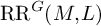
 satisfying the prequantization condition (1.2). In case that G is trivial, it reduces to the classical Riemann-Roch number
$\text {RR}(M,L)$
satisfying the prequantization condition (1.2). In case that G is trivial, it reduces to the classical Riemann-Roch number
$\text {RR}(M,L)$
 , which is computed by the celebrated Hirzebruch-Riemann-Roch formula

where the closed form
$\operatorname {\mathrm {Td}}(M)\in \Omega ^*(M,{\mathbb C})$
 of mixed degrees is the Todd form of
$(M,J,g^{TM})$
of mixed degrees is the Todd form of
$(M,J,g^{TM})$
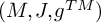 , whose cohomology class does not depend on J and hence is a symplectic invariant of
$(M,\omega )$
, whose cohomology class does not depend on J and hence is a symplectic invariant of
$(M,\omega )$
 .
.
In case of a general G, if
$0$
 does not belong to the image of the moment map, then
${\mathscr M}_0=\emptyset $
does not belong to the image of the moment map, then
${\mathscr M}_0=\emptyset $
 and
$\text {RR}^G(M,L)=0$
and
$\text {RR}^G(M,L)=0$
 . If
$0$
. If
$0$
 is a regular value of the moment map
${ \mathcal J}$
is a regular value of the moment map
${ \mathcal J}$
 , the symplectic quotient
$({\mathscr M}_0,\omega _0)$
, the symplectic quotient
$({\mathscr M}_0,\omega _0)$
 is an orbifold prequantized by a line bundle
$(L_0,h^{L_0})$
is an orbifold prequantized by a line bundle
$(L_0,h^{L_0})$
 and by a general result of Meinrenken [Reference Meinrenken29] one has

In the special case
$G=S^1$
 , this was previously established independently by Meinrenken in [Reference Meinrenken28, Theorem 2.1, (16)] and by Vergne in [Reference Vergne40]. As explained in [Reference Vergne40], these results rely on localization formulas for certain oscillatory integrals of equivariant differential forms which were first studied by Witten in [Reference Witten41], based on previous work of Duistermaat and Heckman in [Reference Duistermaat and Heckman9]. To obtain (1.6) within this approach, one expresses
$\text {RR}^G(M,L)$
, this was previously established independently by Meinrenken in [Reference Meinrenken28, Theorem 2.1, (16)] and by Vergne in [Reference Vergne40]. As explained in [Reference Vergne40], these results rely on localization formulas for certain oscillatory integrals of equivariant differential forms which were first studied by Witten in [Reference Witten41], based on previous work of Duistermaat and Heckman in [Reference Duistermaat and Heckman9]. To obtain (1.6) within this approach, one expresses
$\text {RR}^G(M,L)$
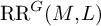 by means of the equivariant Hirzebruch-Riemann-Roch formula in a guise due to Berline and Vergne [Reference Berline and Vergne3], called the Kirillov formula. This formula involves the equivariant Todd form
$\operatorname {\mathrm {Td}}_{\mathbf {\mathfrak g}}(M)\in \Omega ^*_G(M)$
by means of the equivariant Hirzebruch-Riemann-Roch formula in a guise due to Berline and Vergne [Reference Berline and Vergne3], called the Kirillov formula. This formula involves the equivariant Todd form
$\operatorname {\mathrm {Td}}_{\mathbf {\mathfrak g}}(M)\in \Omega ^*_G(M)$
 defined in Section 2.3, whose cohomology class in the equivariant cohomology with analytic coefficients
$H^*_G(M)$
defined in Section 2.3, whose cohomology class in the equivariant cohomology with analytic coefficients
$H^*_G(M)$
 is an invariant of the Hamiltonian G-action on
$(M,\omega )$
is an invariant of the Hamiltonian G-action on
$(M,\omega )$
 . The resulting expression for
$\text {RR}^G(M,L)$
. The resulting expression for
$\text {RR}^G(M,L)$
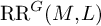 is given in terms of a Witten integral, which can then be treated using the stationary phase principle. In doing so, one passes from the equivariant cohomology
$H^*_G(M)$
is given in terms of a Witten integral, which can then be treated using the stationary phase principle. In doing so, one passes from the equivariant cohomology
$H^*_G(M)$
 to the usual cohomology
$H^*({\mathscr M}_0)$
to the usual cohomology
$H^*({\mathscr M}_0)$
 of the symplectic quotient through the well-known Kirwan map
$\kappa :H^*_G(M)\to H^*({\mathscr M}_0)$
of the symplectic quotient through the well-known Kirwan map
$\kappa :H^*_G(M)\to H^*({\mathscr M}_0)$
 described in Proposition 4.1. Since in the case
$G=S^1$
described in Proposition 4.1. Since in the case
$G=S^1$
 one has
$\kappa (\operatorname {\mathrm {Td}}_{\mathbf {\mathfrak g}}(M))=\operatorname {\mathrm {Td}}({\mathscr M}_0)$
one has
$\kappa (\operatorname {\mathrm {Td}}_{\mathbf {\mathfrak g}}(M))=\operatorname {\mathrm {Td}}({\mathscr M}_0)$
 , this gives the first equality in (1.6), while the second follows from (1.5).
In this paper, we are mainly interested in the considerably more involved case when
$0$
 is a singular value of the moment map and restrict ourselves to the case
$G=S^1$
is a singular value of the moment map and restrict ourselves to the case
$G=S^1$
 , which already encompasses essential features of the singular case. Denoting by
$M^{S^1}\subset M$
, which already encompasses essential features of the singular case. Denoting by
$M^{S^1}\subset M$
 the set of fixed points of the
$S^1$
the set of fixed points of the
$S^1$
 -action and setting
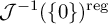
${ \mathcal J}^{-1}(\left \{ \mathrm {0} \right \})^{\text {reg}}:={ \mathcal J}^{-1}(\left \{ \mathrm {0} \right \})\setminus \big ( M^{S^1} \cap { \mathcal J}^{-1}(\{0\})\big )$
-action and setting
${ \mathcal J}^{-1}(\left \{ \mathrm {0} \right \})^{\text {reg}}:={ \mathcal J}^{-1}(\left \{ \mathrm {0} \right \})\setminus \big ( M^{S^1} \cap { \mathcal J}^{-1}(\{0\})\big )$
 we have a stratification of
${ \mathcal J}^{-1}(\{0\})$
we have a stratification of
${ \mathcal J}^{-1}(\{0\})$
 according to

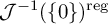
where the connected components of each stratum are smooth submanifolds of M. To avoid any artificial complications, we will assume for simplicity that
$S^1$
 acts freely on
${ \mathcal J}^{-1}(\left \{ \mathrm {0} \right \})^{\text {reg}}$
acts freely on
${ \mathcal J}^{-1}(\left \{ \mathrm {0} \right \})^{\text {reg}}$
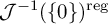 , so that the regular stratum of the symplectic quotient, defined by

has no orbifold singularities. We still write
$\omega _0$
 for the symplectic form over the smooth stratum
${\mathscr M}_0^{\text {reg}}$
for the symplectic form over the smooth stratum
${\mathscr M}_0^{\text {reg}}$
 characterized by the formula
$\text {inc}^*_0\,\omega =\pi _0^*\,\omega _0$
characterized by the formula
$\text {inc}^*_0\,\omega =\pi _0^*\,\omega _0$
 , where
${\text {inc}_0:{ \mathcal J}^{-1}(\left \{ \mathrm {0} \right \})^{\text {reg}}\hookrightarrow M}$
, where
${\text {inc}_0:{ \mathcal J}^{-1}(\left \{ \mathrm {0} \right \})^{\text {reg}}\hookrightarrow M}$
 is the inclusion map and
$\pi _0:{ \mathcal J}^{-1}(\left \{ \mathrm {0} \right \})^{\text {reg}}\to {\mathscr M}_0^{\text {reg}}$
is the inclusion map and
$\pi _0:{ \mathcal J}^{-1}(\left \{ \mathrm {0} \right \})^{\text {reg}}\to {\mathscr M}_0^{\text {reg}}$
 the quotient map. Similarly, the singular stratum
$M^{S^1}\cap { \mathcal J}^{-1}(\{0\})$
the quotient map. Similarly, the singular stratum
$M^{S^1}\cap { \mathcal J}^{-1}(\{0\})$
 of the symplectic quotient carries a symplectic structure by restriction of
$\omega $
of the symplectic quotient carries a symplectic structure by restriction of
$\omega $
 .
.
By a classical result of Kirwan [Reference Kirwan21], we know that the fibers of the moment map are connected, so that if
$0$
 is a local extremal value of
${ \mathcal J}:M\to {\mathbb R}$
is a local extremal value of
${ \mathcal J}:M\to {\mathbb R}$
 , one infers with the local normal form theorem of Proposition 3.2 that
${ \mathcal J}^{-1}(\left \{ \mathrm {0} \right \})=M^{S^1}\cap { \mathcal J}^{-1}(\left \{ \mathrm {0} \right \})$
, one infers with the local normal form theorem of Proposition 3.2 that
${ \mathcal J}^{-1}(\left \{ \mathrm {0} \right \})=M^{S^1}\cap { \mathcal J}^{-1}(\left \{ \mathrm {0} \right \})$
 , which is thus a symplectic submanifold of
$(M,\omega )$
, which is thus a symplectic submanifold of
$(M,\omega )$
 . Since symplectic submanifolds are of codimension
$2$
. Since symplectic submanifolds are of codimension
$2$
 , the mean value theorem implies that
$0$
, the mean value theorem implies that
$0$
 lies on the boundary
$\partial \,{ \mathcal J}(M)$
lies on the boundary
$\partial \,{ \mathcal J}(M)$
 of the image of
${ \mathcal J}$
of the image of
${ \mathcal J}$
 and is consequently a global extremal value of
${ \mathcal J}$
and is consequently a global extremal value of
${ \mathcal J}$
 . In this case the quotient (1.1) satisfies
${\mathscr M}_0={ \mathcal J}^{-1}(\left \{ \mathrm {0} \right \})$
. In this case the quotient (1.1) satisfies
${\mathscr M}_0={ \mathcal J}^{-1}(\left \{ \mathrm {0} \right \})$
 and inherits a natural prequantizing line bundle
$(L_0,h^{L_0})$
and inherits a natural prequantizing line bundle
$(L_0,h^{L_0})$
 by restriction. The invariant Hirzebruch-Riemann-Roch formula (1.6) was then established by Duistermaat, Guillemin, Meinrenken and Wu in [Reference Duistermaat, Guillemin, Meinrenken and Wu8, § 2]. Therefore, the main case of interest in this paper is when
$0$
by restriction. The invariant Hirzebruch-Riemann-Roch formula (1.6) was then established by Duistermaat, Guillemin, Meinrenken and Wu in [Reference Duistermaat, Guillemin, Meinrenken and Wu8, § 2]. Therefore, the main case of interest in this paper is when
$0$
 lies in the interior
$\text {Int}\,{ \mathcal J}(M)$
lies in the interior
$\text {Int}\,{ \mathcal J}(M)$
 of the image of
${ \mathcal J}$
of the image of
${ \mathcal J}$
 , in which case
$0$
, in which case
$0$
 is not a local extremal value of
${ \mathcal J}$
is not a local extremal value of
${ \mathcal J}$
 .
.
Following Notation 3.1, let us write
${\mathcal F}^0$
 for the set of connected components of
$M^{S^1}\cap { \mathcal J}^{-1}(\{0\})$
for the set of connected components of
$M^{S^1}\cap { \mathcal J}^{-1}(\{0\})$
 . For any
$F\in \mathcal {F}^0$
. For any
$F\in \mathcal {F}^0$
 , let
$\omega _F:=\mathrm {inc}_F^\ast \,\omega \in \Omega ^2(F,{\mathbb R})$
, let
$\omega _F:=\mathrm {inc}_F^\ast \,\omega \in \Omega ^2(F,{\mathbb R})$
 be the symplectic form on
$F\subset M$
be the symplectic form on
$F\subset M$
 induced by the inclusion
$\mathrm {inc}_F:F \hookrightarrow M$
induced by the inclusion
$\mathrm {inc}_F:F \hookrightarrow M$
 , and let
$\nu _{\Sigma _F}:\Sigma _F\to F$
, and let
$\nu _{\Sigma _F}:\Sigma _F\to F$
 be the associated symplectic normal bundle. We write

for its decomposition into isotypic components with respect to the induced linear
$S^1$
 -action, where
$W\subset {\mathbb Z}$
-action, where
$W\subset {\mathbb Z}$
 denotes the finite subset of weights as described in Section 3.1. The compatible almost complex structure
$J\in \operatorname {\mathrm {End}}(TM)$
denotes the finite subset of weights as described in Section 3.1. The compatible almost complex structure
$J\in \operatorname {\mathrm {End}}(TM)$
 over
$(M,\omega )$
over
$(M,\omega )$
 and the associated Riemannian metric
$g^{TM}$
and the associated Riemannian metric
$g^{TM}$
 given by (1.3) induce for each weight
$k\in W\subset {\mathbb Z}$
given by (1.3) induce for each weight
$k\in W\subset {\mathbb Z}$
 a complex structure and Hermitian norm
$\|\cdot \|_F$
a complex structure and Hermitian norm
$\|\cdot \|_F$
 on
$\Sigma _F^{(k)}$
on
$\Sigma _F^{(k)}$
 by restriction, and we write
$R^{\Sigma _F^{(k)}}\in \Omega ^2(F,\operatorname {\mathrm {End}}(\Sigma _F^{(k)}))$
by restriction, and we write
$R^{\Sigma _F^{(k)}}\in \Omega ^2(F,\operatorname {\mathrm {End}}(\Sigma _F^{(k)}))$
 for the curvature of the connection on
$\Sigma _F^{(k)}$
for the curvature of the connection on
$\Sigma _F^{(k)}$
 induced by the Levi-Civita connection of
$g^{TM}$
induced by the Levi-Civita connection of
$g^{TM}$
 for each
$k\in W$
for each
$k\in W$
 .
.
Let us now consider the case
$0\in \operatorname {\mathrm {Int}}{ \mathcal J}(M)$
 , and for any
$F\in {\mathcal F}^0$
, and for any
$F\in {\mathcal F}^0$
 , consider the fiberwise product

where
$S_F^\pm \to F$
 are the unit sphere bundles of the subbundles
$\Sigma _F^\pm \subset \Sigma _F$
are the unit sphere bundles of the subbundles
$\Sigma _F^\pm \subset \Sigma _F$
 of positive and negative weights, respectively. By the local normal form theorem of Proposition 3.2, the total space of
$S_F$
of positive and negative weights, respectively. By the local normal form theorem of Proposition 3.2, the total space of
$S_F$
 is naturally identified with the boundary of a neighborhood of F inside
${ \mathcal J}^{-1}(\left \{ \mathrm {0} \right \})$
is naturally identified with the boundary of a neighborhood of F inside
${ \mathcal J}^{-1}(\left \{ \mathrm {0} \right \})$
 . We write

for the orbifold bundle obtained by taking the fiberwise product of the quotient of each sphere by the induced locally free
$S^1$
 -action. Its de Rham cohomology ring will be denoted by
$H^*(\mathfrak {S}_F)$
-action. Its de Rham cohomology ring will be denoted by
$H^*(\mathfrak {S}_F)$
 .
.
Our main result is the following Hirzebruch-Riemann-Roch type formula for the invariant Riemann-Roch number (1.4).
Theorem 1.1. Let
$(M,\omega ,{ \mathcal J})$
 be a compact connected prequantized Hamiltonian
$S^1$
be a compact connected prequantized Hamiltonian
$S^1$
 -manifold such that
$0 \in { \mathcal J}(M)$
-manifold such that
$0 \in { \mathcal J}(M)$
 and the
$S^1$
and the
$S^1$
 -action is free on
${ \mathcal J}^{-1}(\left \{ \mathrm {0} \right \})^{\text {reg}}$
-action is free on
${ \mathcal J}^{-1}(\left \{ \mathrm {0} \right \})^{\text {reg}}$
 . Then, the
$S^1$
. Then, the
$S^1$
 -invariant Riemann-Roch number (1.4) is given by

where
$\kappa :\Omega _{S^1}^*(M)\longrightarrow \Omega ^*({\mathscr M}_0^{\mathrm {reg}},{\mathbb C})$
 denotes the regular Kirwan map of Definition 4.3 and
$\kappa _F:H_{S^1}^*(M)\to H^*(\mathfrak {S}_F)$
denotes the regular Kirwan map of Definition 4.3 and
$\kappa _F:H_{S^1}^*(M)\to H^*(\mathfrak {S}_F)$
 the exceptional Kirwan map (1.12), and

while
$\text {Res}$
 stands for the residue at
$z=0$
stands for the residue at
$z=0$
 if
$0$
if
$0$
 is a minimal value of
${ \mathcal J}$
is a minimal value of
${ \mathcal J}$
 , the residue at
$z=\infty $
, the residue at
$z=\infty $
 if
$0$
if
$0$
 is a maximal value of
${ \mathcal J}$
is a maximal value of
${ \mathcal J}$
 , or the average of the two residues otherwise.
Furthermore, every term on the right-hand side of Formula (1.10) is independent of the choice of a compatible almost complex structure
$J\in \operatorname {\mathrm {End}}(TM)$
 over
$(M,\omega )$
over
$(M,\omega )$
 and of the choice of
$(L,h^L,\nabla ^L)$
and of the choice of
$(L,h^L,\nabla ^L)$
 satisfying the prequantization condition (1.2).
The first term of formula (1.10) is called the regular term, and the convergence of this integral over the non-compact manifold
${\mathscr M}_0^{\mathrm {reg}}$
 will be established in Lemma 4.4. As we explain in more detail below, Theorem 1.1 represents an instance of the Guillemin-Sternberg principle in the singular case and is characterized by the novel conceptual feature that it expresses the invariant Riemann-Roch number purely in terms of the symplectic invariants of the singular symplectic quotient
${\mathscr M}_0$
will be established in Lemma 4.4. As we explain in more detail below, Theorem 1.1 represents an instance of the Guillemin-Sternberg principle in the singular case and is characterized by the novel conceptual feature that it expresses the invariant Riemann-Roch number purely in terms of the symplectic invariants of the singular symplectic quotient
${\mathscr M}_0$
 . In particular, replacing L by the tensor power
$L^m:=L^{\otimes m}$
. In particular, replacing L by the tensor power
$L^m:=L^{\otimes m}$
 for any
$m\in {\mathbb N}$
for any
$m\in {\mathbb N}$
 , so that the symplectic form
$\omega $
, so that the symplectic form
$\omega $
 is replaced by
$m\omega $
is replaced by
$m\omega $
 , one sees that each term of the right-hand side of Formula (1.10) for
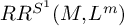
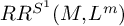
$RR^{S^1}(M,L^m)$
, one sees that each term of the right-hand side of Formula (1.10) for
$RR^{S^1}(M,L^m)$
 is polynomial in
$m\in {\mathbb N}$
is polynomial in
$m\in {\mathbb N}$
 , and Theorem 1.1 thus gives explicit formulas to compute the coefficients of
$RR^{S^1}(M,L^m)$
, and Theorem 1.1 thus gives explicit formulas to compute the coefficients of
$RR^{S^1}(M,L^m)$
 as a polynomial in
$m\in {\mathbb N}$
as a polynomial in
$m\in {\mathbb N}$
 in terms of symplectic invariants of
${\mathscr M}_0$
in terms of symplectic invariants of
${\mathscr M}_0$
 . Let us also point out that Theorem 1.1 is already relevant in the complex case, giving an explicit formula for the coordinate ring of singular projective varieties
${\mathscr M}_0$
. Let us also point out that Theorem 1.1 is already relevant in the complex case, giving an explicit formula for the coordinate ring of singular projective varieties
${\mathscr M}_0$
 obtained as GIT quotients by a
${\mathbb C}^*$
obtained as GIT quotients by a
${\mathbb C}^*$
 -action of a smooth projective variety M.
In case that
$0$
 is a regular value of the moment map
${ \mathcal J}$
is a regular value of the moment map
${ \mathcal J}$
 one has
$M^{S^1}\cap { \mathcal J}^{-1}(\left \{ \mathrm {0} \right \})=\emptyset $
one has
$M^{S^1}\cap { \mathcal J}^{-1}(\left \{ \mathrm {0} \right \})=\emptyset $
 , the last two terms of Formula (1.10) vanish and Theorem 1.1 reduces to the invariant Riemann-Roch formula (1.6), as already explained there. At the other extreme end, in the case when
$0\in \partial \,{ \mathcal J}$
, the last two terms of Formula (1.10) vanish and Theorem 1.1 reduces to the invariant Riemann-Roch formula (1.6), as already explained there. At the other extreme end, in the case when
$0\in \partial \,{ \mathcal J}$
 , we have
${ \mathcal J}^{-1}(\left \{ \mathrm {0} \right \})=M^{S^1}\cap { \mathcal J}^{-1}(\left \{ \mathrm {0} \right \})$
, we have
${ \mathcal J}^{-1}(\left \{ \mathrm {0} \right \})=M^{S^1}\cap { \mathcal J}^{-1}(\left \{ \mathrm {0} \right \})$
 and the first two terms of Formula (1.10) vanish. Theorem 1.1 then yields again (1.6) by taking into account that all weights
$k\in W$
and the first two terms of Formula (1.10) vanish. Theorem 1.1 then yields again (1.6) by taking into account that all weights
$k\in W$
 of the
$S^1$
of the
$S^1$
 -action on
$\Sigma _F$
-action on
$\Sigma _F$
 are of the same sign, its proof reducing to the original proof of Duistermaat, Guillemin, Meinrenken and Wu in [Reference Duistermaat, Guillemin, Meinrenken and Wu8, § 2]. Theorem 1.1 can thus be seen as an interpolation between these two extreme cases which covers also the genuinely singular case. In particular, the middle term in Formula (1.10) appears to be a previously unknown object involving a new explicit symplectic invariant of the singularities.
To describe this term more closely, let
$\Theta ^\pm _{S_F}\in \Omega ^1(S_F,{\mathbb R})$
 be the pullbacks to (1.8) of connections for the
$S^1$
be the pullbacks to (1.8) of connections for the
$S^1$
 -actions on
$S_F^\pm $
-actions on
$S_F^\pm $
 in the sense of (2.8) for any
$F\in {\mathcal F}^0$
in the sense of (2.8) for any
$F\in {\mathcal F}^0$
 . At the level of
$S^1$
. At the level of
$S^1$
 -equivariant differential forms as in Definition (2.7) and using the same notation as for the Kirwan map (4.1), the image of an equivariantly closed form
$\varrho \in \Omega ^*_{S^1}(M)$
-equivariant differential forms as in Definition (2.7) and using the same notation as for the Kirwan map (4.1), the image of an equivariantly closed form
$\varrho \in \Omega ^*_{S^1}(M)$
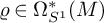 by the exceptional Kirwan map is the element in
$\Omega ^*(\mathfrak {S}_F,{\mathbb C})$
by the exceptional Kirwan map is the element in
$\Omega ^*(\mathfrak {S}_F,{\mathbb C})$
 defined by

where we wrote
$\varrho _{S_F}:=\nu _{S_F}^\ast \mathrm {inc}_F^\ast \varrho \in \Omega ^*_{S^1}(S_F)$
 for the pullback to
$S_F$
for the pullback to
$S_F$
 of the restriction of
$\varrho $
of the restriction of
$\varrho $
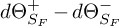
 to F. The numerator on the right-hand side of (1.12) is a multiple of
$d \Theta _{S_F}^+-d \Theta _{S_F }^-$
to F. The numerator on the right-hand side of (1.12) is a multiple of
$d \Theta _{S_F}^+-d \Theta _{S_F }^-$
 inside the ring
$\Omega ^*(S_F,{\mathbb C})$
inside the ring
$\Omega ^*(S_F,{\mathbb C})$
 , which gives an obvious sense to the fraction. Hence, as it is also closed and basic for the action of
$S^1$
, which gives an obvious sense to the fraction. Hence, as it is also closed and basic for the action of
$S^1$
 on both sphere bundles
$S_F^\pm $
on both sphere bundles
$S_F^\pm $
 , by Proposition 2.4, Formula (1.12) induces a well-defined map
$\kappa _F:H_{S^1}^*(M)\to H^*(\mathfrak {S}_F)$
, by Proposition 2.4, Formula (1.12) induces a well-defined map
$\kappa _F:H_{S^1}^*(M)\to H^*(\mathfrak {S}_F)$
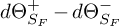
 in cohomology. In fact, the numerator in (1.12) is even a multiple of
$(d \Theta _{S_F}^+-d \Theta _{S_F }^-)^2$
in cohomology. In fact, the numerator in (1.12) is even a multiple of
$(d \Theta _{S_F}^+-d \Theta _{S_F }^-)^2$
 , so that the right-hand side of (1.12) is itself a multiple of
$d \Theta _{S_F}^+-d \Theta _{S_F }^-$
, so that the right-hand side of (1.12) is itself a multiple of
$d \Theta _{S_F}^+-d \Theta _{S_F }^-$
 . This implies in particular that
$\kappa _F$
. This implies in particular that
$\kappa _F$
 , and hence the middle term in Formula (1.10), vanishes when
$\dim M<6$
, and hence the middle term in Formula (1.10), vanishes when
$\dim M<6$
 .
.
The invariant Riemann-Roch formula (1.6) is the content of the celebrated Quantization commutes with Reduction principle of Guillemin and Sternberg, which they formulated in [Reference Guillemin and Sternberg11] in the case of Kähler manifolds, always under the assumption that
$0$
 is a regular value of the moment map. In that case, the kernel of the Spin
$^c$
is a regular value of the moment map. In that case, the kernel of the Spin
$^c$
 -Dirac operator
$D^\pm $
-Dirac operator
$D^\pm $
 reduces to the kernel of the Dolbeault
$\overline \partial $
reduces to the kernel of the Dolbeault
$\overline \partial $
 -operator acting on
$\Omega ^{0,\pm }(M,L)$
-operator acting on
$\Omega ^{0,\pm }(M,L)$
 . In particular, the kernel of the
$\overline \partial $
. In particular, the kernel of the
$\overline \partial $
 -operator restricted to
$\Omega ^{0,0}(M,L)$
-operator restricted to
$\Omega ^{0,0}(M,L)$
 coincides with the space
$H^0(M,L)$
coincides with the space
$H^0(M,L)$
 of holomorphic sections of L over M, which is interpreted in [Reference Guillemin and Sternberg11] as the quantization of the classical phase space
$(M,\omega )$
of holomorphic sections of L over M, which is interpreted in [Reference Guillemin and Sternberg11] as the quantization of the classical phase space
$(M,\omega )$
 . Furthermore,
$0$
. Furthermore,
$0$
 being a regular value, the symplectic reduction
$({\mathscr M}_0,\omega _0)$
being a regular value, the symplectic reduction
$({\mathscr M}_0,\omega _0)$
 inherits a natural structure of a Kähler orbifold, and it was shown in [Reference Guillemin and Sternberg11] that there is a natural isomorphism

The identity (1.13) was generalized to the kernel of the
$\overline \partial $
 -operator restricted to
$\Omega ^{0,j}(M,L)$
-operator restricted to
$\Omega ^{0,j}(M,L)$
 for each
$j>0$
for each
$j>0$
 by Teleman [Reference Teleman37] and Zhang [Reference Zhang42]. Taking the alternating sum of dimensions of these spaces, this precisely leads to the invariant Riemann-Roch formula (1.6) in the context of Kähler manifolds. As we explain in Section 2.2, Formula (1.6) naturally extends to general symplectic manifolds, so that it constitutes the appropriate extension of Quantization commutes with Reduction in the general symplectic case, since the isomorphism (1.13) does not make sense in general. In case that L is replaced by the tensor power
$L^m:=L^{\otimes m}$
by Teleman [Reference Teleman37] and Zhang [Reference Zhang42]. Taking the alternating sum of dimensions of these spaces, this precisely leads to the invariant Riemann-Roch formula (1.6) in the context of Kähler manifolds. As we explain in Section 2.2, Formula (1.6) naturally extends to general symplectic manifolds, so that it constitutes the appropriate extension of Quantization commutes with Reduction in the general symplectic case, since the isomorphism (1.13) does not make sense in general. In case that L is replaced by the tensor power
$L^m:=L^{\otimes m}$
 for
$m\in {\mathbb N}$
for
$m\in {\mathbb N}$
 large enough, Formula (1.6) was established by Meinrenken in [Reference Meinrenken28] by the approach already described above, then by Jeffrey-Kirwan in [Reference Jeffrey and Kirwan18] relying on the so-called Witten non-abelian localization formula stated in [Reference Witten41], which was established rigorously by Jeffrey and Kirwan in [Reference Jeffrey and Kirwan17]. In general, Formula (1.6) was first established by Meinrenken in [Reference Meinrenken29] using the symplectic cutting techniques of Lerman [Reference Lerman24], then by Tian and Zhang [Reference Tian and Zhang38] using the analytic localization techniques of Bismut-Lebeau [Reference Bismut and Lebeau4]. Formula (1.6) was generalized to the case of manifolds with boundary by Tian and Zhang in [Reference Tian and Zhang39], then to the case of non-compact
$(M,\omega )$
large enough, Formula (1.6) was established by Meinrenken in [Reference Meinrenken28] by the approach already described above, then by Jeffrey-Kirwan in [Reference Jeffrey and Kirwan18] relying on the so-called Witten non-abelian localization formula stated in [Reference Witten41], which was established rigorously by Jeffrey and Kirwan in [Reference Jeffrey and Kirwan17]. In general, Formula (1.6) was first established by Meinrenken in [Reference Meinrenken29] using the symplectic cutting techniques of Lerman [Reference Lerman24], then by Tian and Zhang [Reference Tian and Zhang38] using the analytic localization techniques of Bismut-Lebeau [Reference Bismut and Lebeau4]. Formula (1.6) was generalized to the case of manifolds with boundary by Tian and Zhang in [Reference Tian and Zhang39], then to the case of non-compact
$(M,\omega )$
 by Ma and Zhang in [Reference Ma and Zhang27] and Paradan in [Reference Paradan33]. A generalization to compact CR-manifolds was recently established by Ma, Marinescu, and Hsiao in [Reference Hsiao, Ma and Marinescu15].
In case that
$0$
 is a singular value of the moment map, there is an immediate difficulty coming from the fact that there is no natural definition of the Riemann-Roch number
$\text {RR}({\mathscr M}_0,L_0)\in {\mathbb Z}$
is a singular value of the moment map, there is an immediate difficulty coming from the fact that there is no natural definition of the Riemann-Roch number
$\text {RR}({\mathscr M}_0,L_0)\in {\mathbb Z}$
 of a singular symplectic quotient
${\mathscr M}_0$
of a singular symplectic quotient
${\mathscr M}_0$
 , and one is tempted to define it directly as
$\text {RR}({\mathscr M}_0,L_0):=\text {RR}^G(M,L)$
, and one is tempted to define it directly as
$\text {RR}({\mathscr M}_0,L_0):=\text {RR}^G(M,L)$
 , making the result tautological. More substantially, one can consider the Riemann-Roch number of various notions of symplectic desingularization of stratified symplectic spaces, such as Kirwan’s partial desingularization or the shift desingularization. The invariant Riemann-Roch number
$\text {RR}^G(M,L)$
, making the result tautological. More substantially, one can consider the Riemann-Roch number of various notions of symplectic desingularization of stratified symplectic spaces, such as Kirwan’s partial desingularization or the shift desingularization. The invariant Riemann-Roch number
$\text {RR}^G(M,L)$
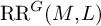 was shown to coincide with the Riemann-Roch number of Kirwan’s partial desingularization by Meinrenken and Sjamaar in [Reference Meinrenken and Sjamaar30], and of the shift desingularization by Meinrenken and Sjamaar in [Reference Meinrenken and Sjamaar30], Zhang in [Reference Zhang42] and Paradan in [Reference Paradan32]. In the case
$G=S^1$
was shown to coincide with the Riemann-Roch number of Kirwan’s partial desingularization by Meinrenken and Sjamaar in [Reference Meinrenken and Sjamaar30], and of the shift desingularization by Meinrenken and Sjamaar in [Reference Meinrenken and Sjamaar30], Zhang in [Reference Zhang42] and Paradan in [Reference Paradan32]. In the case
$G=S^1$
 , Tian and Zhang established in [Reference Tian and Zhang39, Theorem 6.4] an identity in terms of a Riemann-Roch number for shift desingularizations containing a term similar to the last term in Formula (1.10).
A main drawback of the approaches described above is that the desingularization depends on a number of choices and is in no way unique, while the symplectic structure also depends on the choice of an auxiliary parameter
$\varepsilon>0$
 . In particular, these results do not allow to compute
$\text {RR}^G(M,L)$
. In particular, these results do not allow to compute
$\text {RR}^G(M,L)$
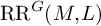 in terms of the symplectic invariants of the symplectic quotient
${\mathscr M}_0$
in terms of the symplectic invariants of the symplectic quotient
${\mathscr M}_0$
 itself and do not provide a canonical Hirzebruch-Riemann-Roch type formula such as (1.6). In contrast, Theorem 1.1 does not rely on any desingularization process and provides an explicit formula for
$\text {RR}^G(M,L)$
itself and do not provide a canonical Hirzebruch-Riemann-Roch type formula such as (1.6). In contrast, Theorem 1.1 does not rely on any desingularization process and provides an explicit formula for
$\text {RR}^G(M,L)$
 in which every term is a well-defined invariant of the Hamiltonian action of
$S^1$
in which every term is a well-defined invariant of the Hamiltonian action of
$S^1$
 on
$(M,\omega )$
on
$(M,\omega )$
 . Thus, our formula satisfies the key requirement of the Guillemin-Sternberg principle that the involved reduced system should only depend on the symplectic data of M, answering an almost 30-year-old question of Sjamaar in [Reference Sjamaar36, pp. 124-126].
In order to compare Theorem 1.1 more closely with the mentioned previous results, we provide in Section 4.2 natural topological conditions on the
$S^1$
 -action under which the first term in (1.10) can be interpreted topologically as

where
$\pi :\widetilde {\mathscr M}_0\to {\mathscr M}_0$
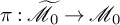 denotes the partial resolution of
${\mathscr M}_0$
denotes the partial resolution of
${\mathscr M}_0$
 and
$\widetilde \omega _0$
and
$\widetilde \omega _0$
 denotes the degenerate
$2$
denotes the degenerate
$2$
 -form over
$\widetilde {\mathscr M}_0$
-form over
$\widetilde {\mathscr M}_0$
 coinciding with
$\omega _0$
coinciding with
$\omega _0$
 on the dense open set
${\mathscr M}_0^{\text {reg}}$
on the dense open set
${\mathscr M}_0^{\text {reg}}$
 , while
$\widetilde \kappa :H^*_{S^1}(M)\longrightarrow H^*(\widetilde {\mathscr M}_0)$
, while
$\widetilde \kappa :H^*_{S^1}(M)\longrightarrow H^*(\widetilde {\mathscr M}_0)$
 is the usual Kirwan map of the resolution. By contrast, the Riemann-Roch formula obtained via the method of Meinrenken and Sjamaar in [Reference Meinrenken and Sjamaar30] reads

where the symplectic form
$\widetilde \omega _{\varepsilon }\in \Omega ^2(\widetilde {\mathscr M}_0,{\mathbb R})$
 depends on the choice of a parameter
$\varepsilon>0$
depends on the choice of a parameter
$\varepsilon>0$
 such that
$\widetilde \omega _{\varepsilon }\xrightarrow {\varepsilon \to 0}\widetilde \omega _0$
such that
$\widetilde \omega _{\varepsilon }\xrightarrow {\varepsilon \to 0}\widetilde \omega _0$
 , while
$\operatorname {\mathrm {Td}}_\varepsilon (\widetilde {\mathscr M}_0)\in \Omega ^\ast (\widetilde {\mathscr M}_0,{\mathbb R})$
, while
$\operatorname {\mathrm {Td}}_\varepsilon (\widetilde {\mathscr M}_0)\in \Omega ^\ast (\widetilde {\mathscr M}_0,{\mathbb R})$
 denotes the induced Todd form. In particular, as
$\widetilde \omega _0$
denotes the induced Todd form. In particular, as
$\widetilde \omega _0$
 is degenerate, the Todd form
$\operatorname {\mathrm {Td}}_\varepsilon (\widetilde {\mathscr M}_0)$
is degenerate, the Todd form
$\operatorname {\mathrm {Td}}_\varepsilon (\widetilde {\mathscr M}_0)$
 does not admit a limit as
$\varepsilon \to 0$
does not admit a limit as
$\varepsilon \to 0$
 , so that the right-hand side is not well defined a priori for
$\varepsilon =0$
, so that the right-hand side is not well defined a priori for
$\varepsilon =0$
 . Let us also point out that Jeffrey, Kiem, Kirwan, and Woolf in [Reference Jeffrey, Kiem, Kirwan and Woolf16], and Lerman and Tolman in [Reference Lerman and Tolman25] in the case of
$G=S^1$
. Let us also point out that Jeffrey, Kiem, Kirwan, and Woolf in [Reference Jeffrey, Kiem, Kirwan and Woolf16], and Lerman and Tolman in [Reference Lerman and Tolman25] in the case of
$G=S^1$
 , studied Kirwan maps to the intersection cohomology of the singular quotient. The relation of their Kirwan maps to our resolution Kirwan map is explained in Remark 4.9.
Our main tool for the proof of Theorem 1.1 is the already mentioned Witten integral, which we introduce in Definition 5.1. In fact, Theorem 1.1 is established as a consequence of our second main result, Theorem 5.7, where we compute an asymptotic expansion of the Witten integral in terms of geometric invariants associated with the singular symplectic quotient. This allows us to directly compute the invariant Riemann-Roch number
$\text {RR}^{S^1}(M,L)$
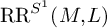 by adapting the method of Meinrenken in [Reference Meinrenken28] to the singular case. The asymptotic parameter in the Witten integral is given by the power
$m\to \infty $
by adapting the method of Meinrenken in [Reference Meinrenken28] to the singular case. The asymptotic parameter in the Witten integral is given by the power
$m\to \infty $
 of the tensor power
$L^m:=L^{\otimes m}$
of the tensor power
$L^m:=L^{\otimes m}$
 of the prequantizing line bundle. It can therefore be regarded as a semiclassical limit, so that from this viewpoint Theorem 1.1 becomes an instance of the correspondence principle of quantum mechanics. Asymptotics of the Witten integral for general Hamiltonian G-manifolds and when
$0$
of the prequantizing line bundle. It can therefore be regarded as a semiclassical limit, so that from this viewpoint Theorem 1.1 becomes an instance of the correspondence principle of quantum mechanics. Asymptotics of the Witten integral for general Hamiltonian G-manifolds and when
$0$
 is a singular value of the moment map were first obtained by Paradan in [Reference Paradan31, Theorem 5.1] relying on partitions of unity in equivariant cohomology with generalized coefficients. There, the coefficients in the expansion are given by integrals over the shifted Marsden-Weinstein reduced spaces
${\mathscr M}_\varepsilon = { \mathcal J}^{-1}(\left \{ \varepsilon \right \})/G$
is a singular value of the moment map were first obtained by Paradan in [Reference Paradan31, Theorem 5.1] relying on partitions of unity in equivariant cohomology with generalized coefficients. There, the coefficients in the expansion are given by integrals over the shifted Marsden-Weinstein reduced spaces
${\mathscr M}_\varepsilon = { \mathcal J}^{-1}(\left \{ \varepsilon \right \})/G$
 for some
$\varepsilon \in \mathbf {\mathfrak g}^\ast $
for some
$\varepsilon \in \mathbf {\mathfrak g}^\ast $
 close to but different from
$0$
close to but different from
$0$
 . In certain algebraic settings, an asymptotic expansion of the Witten integral was also derived by Jeffrey, Kiem, Kirwan, and Woolf in [Reference Jeffrey, Kiem, Kirwan and Woolf16, Section 9] using the localization principle. Accordingly, the coefficients in the asymptotics are given in terms of residues. In contrast, the coefficients in our asymptotic expansion of the Witten integral are given in terms of integrals on the symplectic strata of
${\mathscr M}_0$
. In certain algebraic settings, an asymptotic expansion of the Witten integral was also derived by Jeffrey, Kiem, Kirwan, and Woolf in [Reference Jeffrey, Kiem, Kirwan and Woolf16, Section 9] using the localization principle. Accordingly, the coefficients in the asymptotics are given in terms of residues. In contrast, the coefficients in our asymptotic expansion of the Witten integral are given in terms of integrals on the symplectic strata of
${\mathscr M}_0$
 , which is crucial in proving Theorem 1.1. Our approach was preceded by work of Delarue and Ramacher in [Reference Delarue and Ramacher6] within a purely analytic context, motivated by the original attempt of Ramacher [Reference Ramacher34] of proving residue formulae via singular equivariant asymptotics.
Let us finally note that the assumption of
$S^1$
 acting freely on
${ \mathcal J}^{-1}(\left \{ \mathrm {0} \right \})^{\text {reg}}$
acting freely on
${ \mathcal J}^{-1}(\left \{ \mathrm {0} \right \})^{\text {reg}}$
 , meaning that there are no orbifold singularities over
${\mathscr M}_0^{\text {reg}}$
, meaning that there are no orbifold singularities over
${\mathscr M}_0^{\text {reg}}$
 , is not essential. In fact, the result of Meinrenken in [Reference Meinrenken28], which we extend in this paper to the case when
$0$
, is not essential. In fact, the result of Meinrenken in [Reference Meinrenken28], which we extend in this paper to the case when
$0$
 is a singular value of the moment map, holds for orbifolds as well, and our contribution mainly focuses on the most singular stratum
$M^{S^1}\cap { \mathcal J}^{-1}(\{0\})$
is a singular value of the moment map, holds for orbifolds as well, and our contribution mainly focuses on the most singular stratum
$M^{S^1}\cap { \mathcal J}^{-1}(\{0\})$
 . Following the general method of Meinrenken, one can certainly extend our method to orbifolds, obtaining a Kawasaki-Riemann-Roch type formula which extends (1.10). In a future work, we intend to generalize our results to general compact group actions.
We begin our exposition in Section 2 by giving a detailed account on the background and setup of our paper. In Section 3 we study the geometry of the zero level set of the moment map around its singularities, which will be crucial for the ensuing analysis, and introduce the relevant Kirwan maps in Section 4. Based on these results, we derive in Section 5 a complete asymptotic expansion of the Witten integral. Finally, we establish in Section 6 the proof of our main result Theorem 1.1.
2 Background and setup
Before we introduce our setup, let us first fix some global notation. For any vector bundle E over a smooth manifold M and for all
$k\in {\mathbb N}$
 , we will write
$\Omega ^k(M,E)$
, we will write
$\Omega ^k(M,E)$
 for the space of differential forms of degree k with values in E, and
$\Omega ^*(M,E):=\bigoplus _{k=0}^{\text {dim} M}\Omega ^k(M,E)$
for the space of differential forms of degree k with values in E, and
$\Omega ^*(M,E):=\bigoplus _{k=0}^{\text {dim} M}\Omega ^k(M,E)$
 for the space of differential forms of mixed degrees with values in E. We will use the same notation for any vector space V, which we regard as a trivial vector bundle over M. We will denote the inclusion
$A\hookrightarrow B$
for the space of differential forms of mixed degrees with values in E. We will use the same notation for any vector space V, which we regard as a trivial vector bundle over M. We will denote the inclusion
$A\hookrightarrow B$
 of a subset
$A\subset B$
of a subset
$A\subset B$
 into a set B by
$\mathrm {inc}_A$
into a set B by
$\mathrm {inc}_A$
 , the target set B being clear from the context. For a finite Cartesian product
$X=X_1\times \cdots X_N$
, the target set B being clear from the context. For a finite Cartesian product
$X=X_1\times \cdots X_N$
 , we will write
$\mathrm {pr}_{X_j}:X\to X_j$
, we will write
$\mathrm {pr}_{X_j}:X\to X_j$
 for the canonical projection onto the factor
$X_j$
for the canonical projection onto the factor
$X_j$
 .
.
2.1 Equivariant cohomology
Let M be a smooth manifold equipped with a smooth action of a compact Lie group G. Write
$S^\omega (\mathbf {\mathfrak g}^*)$
 for the complex vector space of analytic series on
$\mathbf {\mathfrak g}$
for the complex vector space of analytic series on
$\mathbf {\mathfrak g}$
 with complex coefficients converging in a neighborhood of
$0\in \mathbf {\mathfrak g}$
with complex coefficients converging in a neighborhood of
$0\in \mathbf {\mathfrak g}$
 . The coadjoint action of G on
$\mathbf {\mathfrak g}^*$
. The coadjoint action of G on
$\mathbf {\mathfrak g}^*$
 induces a natural action on
$S^\omega (\mathbf {\mathfrak g}^*)$
induces a natural action on
$S^\omega (\mathbf {\mathfrak g}^*)$
 .
.
Definition 2.1. The complex of analytic G-equivariant differential forms is the complex vector space of G-invariants

for the natural G-action on the tensor product, equipped with the equivariant differential

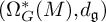
The cohomology of the complex
$(\Omega ^*_G(M),d_{\mathbf {\mathfrak g}})$
 is denoted by
$H^*_G(M)$
is denoted by
$H^*_G(M)$
 and called equivariant cohomology of M with analytic coefficients.
In the above definition and in the sequel, we will often write equivariant differential forms
$\sigma (X)\in \Omega ^*_G(M)$
 with explicit dependence on the variable
$X\in \mathbf {\mathfrak g}$
with explicit dependence on the variable
$X\in \mathbf {\mathfrak g}$
 . We point out that there are several competing conventions for the definition of the equivariant differential in the literature, with the factor
$2\pi i$
. We point out that there are several competing conventions for the definition of the equivariant differential in the literature, with the factor
$2\pi i$
 in (2.1) replaced by other constants. Similarly, the sign in (2.10) is a convention. We follow here Meinrenken’s conventions in [Reference Meinrenken28]. The following version of the Stokes Lemma for equivariant differential forms can be found for instance in [Reference Bott and Tu5, §4].
Lemma 2.2 (Equivariant Stokes’ lemma)
Let
$U\subset M$
 be an open set such that its closure
$\overline U\subset M$
be an open set such that its closure
$\overline U\subset M$
 is a compact submanifold with boundary. Then, for any
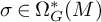
$\sigma \in \Omega ^*_G(M)$
is a compact submanifold with boundary. Then, for any
$\sigma \in \Omega ^*_G(M)$
 we have

For a submanifold
$N\subset M$
 we write
$\nu _{\Sigma _N}:\Sigma _N\to N$
we write
$\nu _{\Sigma _N}:\Sigma _N\to N$
 for its normal bundle inside
$TM$
for its normal bundle inside
$TM$
 and identify N canonically with the zero section in
$\Sigma _N$
and identify N canonically with the zero section in
$\Sigma _N$
 . The following version of the classical homotopy lemma for equivariant differential forms follows for instance from [Reference Goertsches and Zoller10, Theorem 6.1].
Lemma 2.3 (Equivariant homotopy lemma)
Let
$N\subset M$
 be a submanifold preserved by the action of G, and let
$\Phi _N:V_N\to U_N$
be a submanifold preserved by the action of G, and let
$\Phi _N:V_N\to U_N$
 be a G-equivariant diffeomorphism between a tubular neighborhood
$V_N\subset \Sigma _N$
be a G-equivariant diffeomorphism between a tubular neighborhood
$V_N\subset \Sigma _N$
 of the zero section of
$\Sigma _N$
of the zero section of
$\Sigma _N$
 and a tubular neighborhood
$U_N\subset M$
and a tubular neighborhood
$U_N\subset M$
 of N. Then, for any equivariant cohomology class
$[\varrho ] \in H^*_G(M)$
of N. Then, for any equivariant cohomology class
$[\varrho ] \in H^*_G(M)$
 there exists an equivariant form
$\beta _N \in \Omega _{G}^\ast (V_N)$
there exists an equivariant form
$\beta _N \in \Omega _{G}^\ast (V_N)$
 such that

Furthermore, the equivariant form
$\beta _N \in \Omega _{G}^\ast (V_N)$
 can be chosen such that
$\operatorname {{\mathrm {inc}}}_N^*\beta _N\equiv 0$
can be chosen such that
$\operatorname {{\mathrm {inc}}}_N^*\beta _N\equiv 0$
 and such that for any open set
$S\subset V_N$
and such that for any open set
$S\subset V_N$
 on which we already have
$\Phi _{N}^\ast (\varrho |_{U_N})|_{S} = \nu _{\Sigma _N}^\ast \mathrm {inc}_N^*\varrho |_{S}$
on which we already have
$\Phi _{N}^\ast (\varrho |_{U_N})|_{S} = \nu _{\Sigma _N}^\ast \mathrm {inc}_N^*\varrho |_{S}$
 , one has
$\beta _N|_{S}\equiv 0$
, one has
$\beta _N|_{S}\equiv 0$
 .
.
The second part of Lemma 2.3, which will be used in Section 5 to establish Lemma 5.3, follows from the fact that N is a strong deformation retract of
$U_N$
 and the explicit form of the homotopy operator used for instance in [Reference Goertsches and Zoller10, Theorem 6.1] to construct the equivariant form
$\beta _N \in \Omega _{G}^\ast (V_N)$
and the explicit form of the homotopy operator used for instance in [Reference Goertsches and Zoller10, Theorem 6.1] to construct the equivariant form
$\beta _N \in \Omega _{G}^\ast (V_N)$
 of Formula (2.2).
Consider now the important special case when the G-action is locally free, so that the quotient map

is a G-principal bundle over the orbifold
$M/G$
 . We then have the following basic result.
Proposition 2.4. The pullback by the quotient map (2.3) induces an isomorphism of complexes

where the subcomplex of basic differential forms
$\Omega (M)^G_{\mathrm {bas}}\subset \Omega (M,{\mathbb R})$
 is defined by

The cohomology of the complex (2.5) is called the basic cohomology of M, and Proposition 2.4 shows that it is isomorphic to the de Rham cohomology
$H^*(M/G)$
 of the orbifold
$M/G$
of the orbifold
$M/G$
 . On the other hand, one has the following fundamental notion in Chern-Weil theory, which will be of crucial importance in this paper.
Definition 2.5. A connection for a locally free G-action on M is a
$\mathbf {\mathfrak g}$
 -valued
$1$
-valued
$1$
 -form
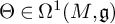
$\Theta \in \Omega ^1(M,\mathbf {\mathfrak g})$
-form
$\Theta \in \Omega ^1(M,\mathbf {\mathfrak g})$
 satisfying for all
$X\in \mathbf {\mathfrak g}$
satisfying for all
$X\in \mathbf {\mathfrak g}$


In what follows, we will mainly be interested in the case where
$G=S^1$
 is the circle group, which we realize as the subgroup of complex numbers of modulus
$1$
is the circle group, which we realize as the subgroup of complex numbers of modulus
$1$
 , inducing an identification

in such a way that
$X\in \mathbf {\mathfrak g}$
 exponentiates to
$e^{2\pi i x}\in S^1\subset {\mathbb C}$
exponentiates to
$e^{2\pi i x}\in S^1\subset {\mathbb C}$
 . This induces in turn an identification
$\mathbf {\mathfrak g}^*\simeq {\mathbb R}$
. This induces in turn an identification
$\mathbf {\mathfrak g}^*\simeq {\mathbb R}$
 of the dual of the Lie algebra with
${\mathbb R}$
of the dual of the Lie algebra with
${\mathbb R}$
 and of the Lebesgue measure on the interval
$[0,1]$
and of the Lebesgue measure on the interval
$[0,1]$
 with the normalized Haar measure on
$S^1$
with the normalized Haar measure on
$S^1$
 . Under this identification, Definition 2.1 becomes

the complex vector space of
$S^1$
 -invariant differential forms with values in entire analytic series of the variable
$x\in {\mathbb R}$
-invariant differential forms with values in entire analytic series of the variable
$x\in {\mathbb R}$
 . We will write
$S^1$
. We will write
$S^1$
 -equivariant differential forms
$\sigma (x)\in \Omega ^*_{S^1}(M)$
-equivariant differential forms
$\sigma (x)\in \Omega ^*_{S^1}(M)$
 with explicit dependence in the variable
$x\in {\mathbb R}$
with explicit dependence in the variable
$x\in {\mathbb R}$
 , when they are understood in the identification (2.7), so that they can actually be seen as functions of
$x\in {\mathbb R}$
, when they are understood in the identification (2.7), so that they can actually be seen as functions of
$x\in {\mathbb R}$
 with values in
$S^1$
with values in
$S^1$
 -invariant differential forms. Furthermore, Definition 2.5 of a connection for the
$S^1$
-invariant differential forms. Furthermore, Definition 2.5 of a connection for the
$S^1$
 -action on M becomes under this identification a
$1$
-action on M becomes under this identification a
$1$
 -form
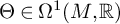
$\Theta \in \Omega ^1(M,{\mathbb R})$
-form
$\Theta \in \Omega ^1(M,{\mathbb R})$
 such that for any
$X\in \mathbf {\mathfrak g}$
such that for any
$X\in \mathbf {\mathfrak g}$
 with image
$x\in {\mathbb R}$
with image
$x\in {\mathbb R}$
 by (2.6), we have

The following basic lemma is then a straightforward consequence of Proposition 2.4 and Definition 2.5 via the identification (2.6).
Lemma 2.6. Assume that the
$S^1$
 -action on M is locally free, let
$\Theta \in \Omega ^1(M,{\mathbb R})$
-action on M is locally free, let
$\Theta \in \Omega ^1(M,{\mathbb R})$
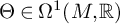 be an associated connection in the sense of (2.8), and let
$\sigma \in \Omega (M/S^1)$
be an associated connection in the sense of (2.8), and let
$\sigma \in \Omega (M/S^1)$
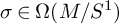 be closed. Then we have

in terms of the isomorphism of complexes (2.4). In particular, the integral on the left-hand side of (2.9) only depends on the basic cohomology class of
$\sigma $
 .
.
2.2 Dirac operators and invariant Riemann-Roch numbers
To introduce our proper setup, let us now focus on the case of a Hamiltonian G-action on a compact connected symplectic manifold
$(M,\omega )$
 of dimension
$2n$
of dimension
$2n$
 . Recall that a G-equivariant map
${ \mathcal J}: M \to \mathbf {\mathfrak g}^\ast $
. Recall that a G-equivariant map
${ \mathcal J}: M \to \mathbf {\mathfrak g}^\ast $
 is called a moment map for such an action if for all
$X\in \mathbf {\mathfrak g}$
is called a moment map for such an action if for all
$X\in \mathbf {\mathfrak g}$
 , the function
${ \mathcal J}(X)\in \mathrm {C^{\infty }}(M,{\mathbb R})$
, the function
${ \mathcal J}(X)\in \mathrm {C^{\infty }}(M,{\mathbb R})$
 satisfies

where d is the de Rham differential and
$\mathbin {\lrcorner }$
 denotes the contraction. By definition, a Hamiltonian G-action on a symplectic manifold
$(M,\omega )$
denotes the contraction. By definition, a Hamiltonian G-action on a symplectic manifold
$(M,\omega )$
 induces a locally free action on the level set
${ \mathcal J}^{-1}(\{0\})$
induces a locally free action on the level set
${ \mathcal J}^{-1}(\{0\})$
 if and only if
$0$
if and only if
$0$
 is a regular value of
${ \mathcal J}:M\to \mathbf {\mathfrak g}^*$
is a regular value of
${ \mathcal J}:M\to \mathbf {\mathfrak g}^*$
 . For
$G=S^1$
. For
$G=S^1$
 , under the identification (2.6) the moment map
${ \mathcal J}:M\to \mathbf {\mathfrak g}^*$
, under the identification (2.6) the moment map
${ \mathcal J}:M\to \mathbf {\mathfrak g}^*$
 corresponds to a function
${ \mathcal J}\in \mathrm {C^{\infty }}(M,{\mathbb R})$
corresponds to a function
${ \mathcal J}\in \mathrm {C^{\infty }}(M,{\mathbb R})$
 which we still call moment map, such that for any
$X\in \mathbf {\mathfrak g}$
which we still call moment map, such that for any
$X\in \mathbf {\mathfrak g}$
 with image
$x\in {\mathbb R}$
with image
$x\in {\mathbb R}$
 by (2.6), we have

Next, let
$(M,\omega )$
 be endowed with a so-called prequantizing line bundle
$(L,h^L,\nabla ^L)$
be endowed with a so-called prequantizing line bundle
$(L,h^L,\nabla ^L)$
 , so that
$(L,h^L)$
, so that
$(L,h^L)$
 is a Hermitian line bundle over M with a Hermitian connection
$\nabla ^L$
is a Hermitian line bundle over M with a Hermitian connection
$\nabla ^L$
 whose curvature
$R^L\in \Omega ^2(M,{\mathbb C})$
whose curvature
$R^L\in \Omega ^2(M,{\mathbb C})$
 satisfies the prequantization condition (1.2). We denote by
$\mathrm {C^{\infty }}(M,L)$
satisfies the prequantization condition (1.2). We denote by
$\mathrm {C^{\infty }}(M,L)$
 the space of smooth sections of L. Let further G be a connected compact Lie group such that G acts on L over M, preserving the Hermitian metric
$h^L$
the space of smooth sections of L. Let further G be a connected compact Lie group such that G acts on L over M, preserving the Hermitian metric
$h^L$
 and the connection
$\nabla ^L$
and the connection
$\nabla ^L$
 . Such an action is called prequantized, and the induced action of G on
$(M,\omega )$
. Such an action is called prequantized, and the induced action of G on
$(M,\omega )$
 then preserves the symplectic form
$\omega $
then preserves the symplectic form
$\omega $
 . Following for instance [Reference Meinrenken28, (25)] adapted to our conventions, there is a canonical choice of moment map
${ \mathcal J}: M \to \mathbf {\mathfrak g}^\ast $
. Following for instance [Reference Meinrenken28, (25)] adapted to our conventions, there is a canonical choice of moment map
${ \mathcal J}: M \to \mathbf {\mathfrak g}^\ast $
 for a prequantized action of G on
$(M,\omega )$
for a prequantized action of G on
$(M,\omega )$
 defined by the Kostant formula

for all
$s\in \mathrm {C^{\infty }}(M,L)$
 and
$X\in \mathbf {\mathfrak g}$
and
$X\in \mathbf {\mathfrak g}$
 , where
$\widetilde X\in \mathrm {C^{\infty }}(M,TM)$
, where
$\widetilde X\in \mathrm {C^{\infty }}(M,TM)$
 denotes the fundamental vector field on M associated with X and
$L_X$
denotes the fundamental vector field on M associated with X and
$L_X$
 denotes the Lie derivative with respect to X induced by the G-action. This is the moment map which will underlie all our considerations from now on.
Next, choose a G-invariant compatible almost complex structure
$J\in \operatorname {\mathrm {End}}(TM)$
 over
$(M,\omega )$
over
$(M,\omega )$
 , inducing a splitting

on the complexification
$TM\otimes {\mathbb C}$
 of
$TM$
of
$TM$
 into the eigenspaces of J corresponding to the eigenvalues i and
$-i$
into the eigenspaces of J corresponding to the eigenvalues i and
$-i$
 , respectively. Consider the total exterior product

where
$T^{*(0,1)}M$
 denotes the dual bundle of
$T^{(0,1)}M$
denotes the dual bundle of
$T^{(0,1)}M$
 . For any
$v\in TM$
. For any
$v\in TM$
 with decomposition
$v=v^{1,0}+v^{0,1}$
with decomposition
$v=v^{1,0}+v^{0,1}$
 according to (2.13), we define its Clifford action on
$\alpha \in \Lambda ( T^{*(0,1)}M)$
according to (2.13), we define its Clifford action on
$\alpha \in \Lambda ( T^{*(0,1)}M)$
 by
by

where
$(v^{1,0})^*$
 denotes the metric dual of
$v^{1,0}$
denotes the metric dual of
$v^{1,0}$
 in
$T^{*(0,1)}M$
in
$T^{*(0,1)}M$
 with respect to the induced Hermitian metric
$g^{TM}$
with respect to the induced Hermitian metric
$g^{TM}$
 defined by (1.3). As explained for instance in [Reference Lawson and Michelsohn23, Appendix D], the Clifford action (2.15) on
$\Lambda ( T^{*(0,1)}M)$
defined by (1.3). As explained for instance in [Reference Lawson and Michelsohn23, Appendix D], the Clifford action (2.15) on
$\Lambda ( T^{*(0,1)}M)$
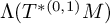 is associated with the canonical
$\mathrm {Spin}^c$
is associated with the canonical
$\mathrm {Spin}^c$
 structure of the almost Hermitian manifold
$(M,J,g^{TM})$
structure of the almost Hermitian manifold
$(M,J,g^{TM})$
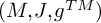 , and there is an induced connection
$\nabla ^{\Lambda ( T^{*(0,1)}M)}$
, and there is an induced connection
$\nabla ^{\Lambda ( T^{*(0,1)}M)}$
 on
$\Lambda ( T^{*(0,1)}M)$
on
$\Lambda ( T^{*(0,1)}M)$
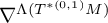
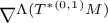
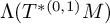 , which we call the Clifford connection. Following [Reference Ma and Marinescu26, §1.3.1], the Clifford connection
$\nabla ^{\Lambda ( T^{*(0,1)}M)}$
, which we call the Clifford connection. Following [Reference Ma and Marinescu26, §1.3.1], the Clifford connection
$\nabla ^{\Lambda ( T^{*(0,1)}M)}$
 is given in any local orthonormal frame
$\{e_j\}_{j=1}^n$
is given in any local orthonormal frame
$\{e_j\}_{j=1}^n$
 of
$(TM,g^{TM})$
of
$(TM,g^{TM})$
 by the formula

where
$\Gamma ^{TM}$
 is the local connection form of the Levi-Civita connection
$\nabla ^{TM}$
is the local connection form of the Levi-Civita connection
$\nabla ^{TM}$
 associated with
$g^{TM}$
associated with
$g^{TM}$
 and
$\Gamma ^{\mathrm {det}\,}$
and
$\Gamma ^{\mathrm {det}\,}$
 is the local connection form associated with the connection on
$\mathrm {det}\,(T^{(1,0)}M):=\Lambda ^n( T^{(1,0)}M)$
is the local connection form associated with the connection on
$\mathrm {det}\,(T^{(1,0)}M):=\Lambda ^n( T^{(1,0)}M)$
 induced by
$\nabla ^{TM}$
induced by
$\nabla ^{TM}$
 . Finally, for any
$m\in {\mathbb N}$
. Finally, for any
$m\in {\mathbb N}$
 , we write
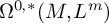
$\Omega ^{0,*}(M,L^m)$
, we write
$\Omega ^{0,*}(M,L^m)$
 for the space of smooth sections of
$\Lambda ( T^{*(0,1)}M)\otimes L^m$
for the space of smooth sections of
$\Lambda ( T^{*(0,1)}M)\otimes L^m$
 , where
$L^m$
, where
$L^m$
 denotes the m-th tensor power of L. We then have the following
Definition 2.7. For any
$m\in {\mathbb N}$
 , the Spin
$^c$
, the Spin
$^c$
 -Dirac operator
$D_m$
-Dirac operator
$D_m$
 is defined in any local orthonormal frame
$\{e_j\}_{j=1}^n$
is defined in any local orthonormal frame
$\{e_j\}_{j=1}^n$
 of
$(TM,g^{TM})$
of
$(TM,g^{TM})$
 by the formula

where
$\nabla ^{\Lambda ( T^{*(0,1)}M)\otimes L^m}$
 is the connection on
$\Lambda ( T^{*(0,1)}M)\otimes L^m$
is the connection on
$\Lambda ( T^{*(0,1)}M)\otimes L^m$
 induced by
$\nabla ^{\Lambda ( T^{*(0,1)}M)}$
induced by
$\nabla ^{\Lambda ( T^{*(0,1)}M)}$
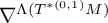 and
$\nabla ^{L^m}$
and
$\nabla ^{L^m}$
 .
.
By definition of the Clifford action (2.15), the
$\mathrm {Spin}^c$
 -Dirac operator
$D_m$
-Dirac operator
$D_m$
 interchanges the space
$\Omega ^{0,+}(M,L^m) \subset \Omega ^{0,*}(M,L^m)$
interchanges the space
$\Omega ^{0,+}(M,L^m) \subset \Omega ^{0,*}(M,L^m)$
 of even-degree forms with the space
$\Omega ^{0,-}(M,L^m)\subset \Omega ^{0,*}(M,L^m)$
of even-degree forms with the space
$\Omega ^{0,-}(M,L^m)\subset \Omega ^{0,*}(M,L^m)$
 of odd-degree forms in the decomposition (2.14) of
$\Lambda ( T^{*(0,1)}M)$
of odd-degree forms in the decomposition (2.14) of
$\Lambda ( T^{*(0,1)}M)$
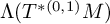 . We write
$D_m^\pm $
. We write
$D_m^\pm $
 for the restriction of
$D_m$
for the restriction of
$D_m$
 to
$\Omega ^{0,\pm }(M,L^m)$
to
$\Omega ^{0,\pm }(M,L^m)$
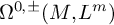 . On the other hand, as shown for instance in [Reference Ma and Marinescu26, Lemma 1.3.4],
$D_m$
. On the other hand, as shown for instance in [Reference Ma and Marinescu26, Lemma 1.3.4],
$D_m$
 is a formally self-adjoint elliptic operator on
$\Omega ^{0,*}(M,L^m)$
is a formally self-adjoint elliptic operator on
$\Omega ^{0,*}(M,L^m)$
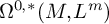 with respect to the
$\mathrm {L}^2$
with respect to the
$\mathrm {L}^2$
 -Hermitian product induced by
$g^{TM}$
-Hermitian product induced by
$g^{TM}$
 and
$h^L$
and
$h^L$
 . In particular, it has finite-dimensional kernel inside
$\Omega ^{0,*}(M,L^m)$
. In particular, it has finite-dimensional kernel inside
$\Omega ^{0,*}(M,L^m)$
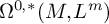 , which allows us to state the following definition.
Definition 2.8. For any
$m\in {\mathbb N}$
 , the Riemann-Roch number
$\text {RR}(M,L^m)\in {\mathbb N}$
, the Riemann-Roch number
$\text {RR}(M,L^m)\in {\mathbb N}$
 of the bundle
$L^m$
of the bundle
$L^m$
 over M is defined by the formula

The standard invariance property of indices of elliptic operators with respect to deformations shows that these Riemann-Roch numbers do not depend on the choice of an almost complex structure J nor on
$h^L$
 and
$\nabla ^L$
and
$\nabla ^L$
 satisfying the prequantization condition (1.2).
On the other hand, recall that the action of G preserves all additional data on M and L by construction, so that there is an induced action of G on
$\Omega ^{0,*}(M,L^m)$
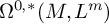 commuting with
$D_m$
commuting with
$D_m$
 . In particular, this induces unitary representations of G on the finite dimensional Hermitian vector spaces
$\operatorname {\mathrm {Ker}} D_m^+$
. In particular, this induces unitary representations of G on the finite dimensional Hermitian vector spaces
$\operatorname {\mathrm {Ker}} D_m^+$
 and
$\operatorname {\mathrm {Ker}} D_m^-$
and
$\operatorname {\mathrm {Ker}} D_m^-$
 . For any
$g\in G$
. For any
$g\in G$
 , we write

We write
$(\operatorname {\mathrm {Ker}} D_m^+)^G$
 and
$(\operatorname {\mathrm {Ker}} D_m^-)^G$
and
$(\operatorname {\mathrm {Ker}} D_m^-)^G$
 for the subspaces of G-invariant vectors inside
$\operatorname {\mathrm {Ker}} D_m^+$
for the subspaces of G-invariant vectors inside
$\operatorname {\mathrm {Ker}} D_m^+$
 and
$\operatorname {\mathrm {Ker}} D_m^-$
and
$\operatorname {\mathrm {Ker}} D_m^-$
 respectively.
Definition 2.9. For any
$m\in {\mathbb N}$
 , the G-invariant Riemann-Roch number
${\text {RR}^G(M,L^m)\in {\mathbb N}}$
, the G-invariant Riemann-Roch number
${\text {RR}^G(M,L^m)\in {\mathbb N}}$
 of the bundle
$L^m$
of the bundle
$L^m$
 over M is defined by the formula

Again by invariance of the index of elliptic operators, the G-invariant Riemann-Roch number does not depend on the choice of a G-invariant almost complex structure J nor on the choice of G-invariant
$h^L$
 and
$\nabla ^L$
and
$\nabla ^L$
 satisfying the prequantization condition (1.2). Note also that we have

where
$dg$
 is the normalized Haar volume form on G.
2.3 Equivariant characteristic forms and Riemann-Roch formulas
In the setting of Section 2.2, and following [Reference Berline, Getzler and Vergne2, Definition 7.5], we define for any Hermitian vector bundle
$(E,h^E)\to M$
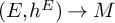 to which the G-action lifts and which is equipped with a G-equivariant Hermitian connection
$\nabla ^E$
to which the G-action lifts and which is equipped with a G-equivariant Hermitian connection
$\nabla ^E$
 the associated moment map
${ \mathcal J}^{E}:M\to \operatorname {\mathrm {End}}(E)\otimes \mathbf {\mathfrak g}^*$
the associated moment map
${ \mathcal J}^{E}:M\to \operatorname {\mathrm {End}}(E)\otimes \mathbf {\mathfrak g}^*$
 via the Kostant formula

where
$L_X$
 denotes the Lie derivative with respect to X induced by the action of G on E. Its equivariant curvature
$R^{E}_{\mathbf {\mathfrak g}}(X)\in \Omega ^*(M,\operatorname {\mathrm {End}}(E))$
denotes the Lie derivative with respect to X induced by the action of G on E. Its equivariant curvature
$R^{E}_{\mathbf {\mathfrak g}}(X)\in \Omega ^*(M,\operatorname {\mathrm {End}}(E))$
 evaluated at
$X\in \mathbf {\mathfrak g}$
evaluated at
$X\in \mathbf {\mathfrak g}$
 is then given by the formula

where
$R^{E}$
 denotes the curvature of
$\nabla ^E$
denotes the curvature of
$\nabla ^E$
 . The associated equivariant Todd form is the equivariantly closed form
$\operatorname {\mathrm {Td}}_{\mathbf {\mathfrak g}}(E)\in \Omega ^*_G(M)$
. The associated equivariant Todd form is the equivariantly closed form
$\operatorname {\mathrm {Td}}_{\mathbf {\mathfrak g}}(E)\in \Omega ^*_G(M)$
 defined for all
$X\in \mathbf {\mathfrak g}$
defined for all
$X\in \mathbf {\mathfrak g}$
 by the formula

One readily checks that its cohomology class in
$H^*_G(M)$
 does not depend on the choice of a Hermitian metric
$h^E$
does not depend on the choice of a Hermitian metric
$h^E$
 and connection
$\nabla ^E$
and connection
$\nabla ^E$
 . In the important case of the tangent bundle
$TM\to M$
. In the important case of the tangent bundle
$TM\to M$
 equipped with the chosen G-invariant compatible almost complex structure
$J\in \operatorname {\mathrm {End}}(TM)$
equipped with the chosen G-invariant compatible almost complex structure
$J\in \operatorname {\mathrm {End}}(TM)$
 over
$(M,\omega )$
over
$(M,\omega )$
 , one can consider the induced Hermitian metric
$g^{TM}$
, one can consider the induced Hermitian metric
$g^{TM}$
 given by Formula (1.3) and the associated Levi-Civita connection
$\nabla ^{TM}$
given by Formula (1.3) and the associated Levi-Civita connection
$\nabla ^{TM}$
 , which are both G-equivariant. This induces a Hermitian metric and connection on
$T^{(1,0)}M$
, which are both G-equivariant. This induces a Hermitian metric and connection on
$T^{(1,0)}M$
 via the splitting (2.13), and the associated equivariant Todd form
$\operatorname {\mathrm {Td}}_{\mathbf {\mathfrak g}}(M)\in \Omega ^*_G(M)$
via the splitting (2.13), and the associated equivariant Todd form
$\operatorname {\mathrm {Td}}_{\mathbf {\mathfrak g}}(M)\in \Omega ^*_G(M)$
 given by
$\operatorname {\mathrm {Td}}_{\mathbf {\mathfrak g}}(M,X):=\operatorname {\mathrm {Td}}_{\mathbf {\mathfrak g}}(T^{(1,0)}M,X)$
given by
$\operatorname {\mathrm {Td}}_{\mathbf {\mathfrak g}}(M,X):=\operatorname {\mathrm {Td}}_{\mathbf {\mathfrak g}}(T^{(1,0)}M,X)$
 does not depend on the choice of the compatible almost complex structure, and hence is an invariant of the Hamiltonian action of G on
$(M,\omega )$
does not depend on the choice of the compatible almost complex structure, and hence is an invariant of the Hamiltonian action of G on
$(M,\omega )$
 . The closed form
$\operatorname {\mathrm {Td}}(M):=\operatorname {\mathrm {Td}}_{\mathbf {\mathfrak g}}(M,0)\in \Omega ^*(M)$
. The closed form
$\operatorname {\mathrm {Td}}(M):=\operatorname {\mathrm {Td}}_{\mathbf {\mathfrak g}}(M,0)\in \Omega ^*(M)$
 is called the Todd form of M, and its cohomology class is a symplectic invariant of
$(M,\omega )$
is called the Todd form of M, and its cohomology class is a symplectic invariant of
$(M,\omega )$
 .
.
Recalling the prequantization condition (1.2), the equivariant Chern character of
$L^m$
 is the equivariantly closed form
$\operatorname {\mathrm {ch}}_{\mathbf {\mathfrak g}}(L^m)\in \Omega ^*_G(M)$
is the equivariantly closed form
$\operatorname {\mathrm {ch}}_{\mathbf {\mathfrak g}}(L^m)\in \Omega ^*_G(M)$
 defined for all
$m\in {\mathbb N}$
defined for all
$m\in {\mathbb N}$
 and
$X\in \mathbf {\mathfrak g}$
and
$X\in \mathbf {\mathfrak g}$
 by the formula

The closed form
$\operatorname {\mathrm {ch}}(L^m):=\operatorname {\mathrm {ch}}_{\mathbf {\mathfrak g}}(L^m,0)=e^{m\omega }\in \Omega ^*(M)$
 is called the Chern character of
$L^m$
is called the Chern character of
$L^m$
 .
.
Consider now for any
$g\in G$
 the fixed point set

which is a smooth submanifold of M, and write
$\Sigma _{M^g}\to M^g$
 for its normal bundle inside
$TM$
for its normal bundle inside
$TM$
 . It is naturally endowed with an action of the centralizer
$Z_g\subset G$
. It is naturally endowed with an action of the centralizer
$Z_g\subset G$
 of g, and we write
$\mathfrak {z}_g$
of g, and we write
$\mathfrak {z}_g$
 for its Lie algebra. Then all of the equivariant characteristic forms considered above make sense for the action of
$Z_g$
for its Lie algebra. Then all of the equivariant characteristic forms considered above make sense for the action of
$Z_g$
 on the vector bundles
$\Sigma _{M^g}$
on the vector bundles
$\Sigma _{M^g}$
 ,
$TM^g$
,
$TM^g$
 , and
$L^m|_{M^g}$
, and
$L^m|_{M^g}$
 over
$M^g$
over
$M^g$
 . In particular, we write
$R^{\Sigma _{M^g}}_{\mathfrak {z}_g}(X)\in \Omega ^2(M^g,\operatorname {\mathrm {End}}(\Sigma _{M^g}))$
. In particular, we write
$R^{\Sigma _{M^g}}_{\mathfrak {z}_g}(X)\in \Omega ^2(M^g,\operatorname {\mathrm {End}}(\Sigma _{M^g}))$
 for the equivariant curvature associated with the connection on
$\Sigma _{M^g}$
for the equivariant curvature associated with the connection on
$\Sigma _{M^g}$
 induced by the Levi-Civita connection of
$g^{TM}$
induced by the Levi-Civita connection of
$g^{TM}$
 .
.
We can now state the following fundamental Kirillov formula, which we present in a guise that can be found in [Reference Meinrenken28, Theorem 3.1 and Remark (4) after Theorem 2.1].
Theorem 2.10. [Reference Berline and Vergne3, Th. 3.23]
For any
$m\in {\mathbb N}$
 ,
$g\in G$
,
$g\in G$
 , and
$X\in \mathfrak {z}_g$
, and
$X\in \mathfrak {z}_g$
 sufficiently close to
$0$
sufficiently close to
$0$
 we have

Note that
$g^{-1}\in G$
 acts fiberwise on the complex line bundle
$L^m|_{M^g}$
acts fiberwise on the complex line bundle
$L^m|_{M^g}$
 by multiplication with a scalar denoted by
$\operatorname {\mathrm {Tr}}_{L^m}[g^{-1}]$
by multiplication with a scalar denoted by
$\operatorname {\mathrm {Tr}}_{L^m}[g^{-1}]$
 in Theorem 2.10. On the one hand, applied to
$g=e$
in Theorem 2.10. On the one hand, applied to
$g=e$
 , the Kirillov formula takes the elegant form

for any
$m\in {\mathbb N}$
 and
$X\in \mathbf {\mathfrak g}$
and
$X\in \mathbf {\mathfrak g}$
 sufficiently close to
$0$
sufficiently close to
$0$
 , compare [Reference Berline, Getzler and Vergne2, Theorem 8.2]. On the other hand, Theorem 2.10 applied to
$X=0$
, compare [Reference Berline, Getzler and Vergne2, Theorem 8.2]. On the other hand, Theorem 2.10 applied to
$X=0$
 recovers the equivariant Atiyah-Segal-Singer index theorem [Reference Atiyah and Segal1]

which is valid for any
$m\in {\mathbb N}$
 and
$g\in G$
and
$g\in G$
 . In particular, Theorem 2.10 applied to
$g=e$
. In particular, Theorem 2.10 applied to
$g=e$
 and
$X=0$
and
$X=0$
 recovers the classical Hirzebruch-Riemann-Roch formula (1.5) for the usual Riemann-Roch numbers of Definition 2.8.
3 Geometry of the zero level set of the moment map
Let
$(M,\omega )$
 be a compact symplectic manifold of dimension
$2n$
be a compact symplectic manifold of dimension
$2n$
 on which
$G=S^1$
on which
$G=S^1$
 acts in a Hamiltonian fashion with moment map
${ \mathcal J}: M \to \mathbf {\mathfrak g}^\ast \simeq {\mathbb R}$
acts in a Hamiltonian fashion with moment map
${ \mathcal J}: M \to \mathbf {\mathfrak g}^\ast \simeq {\mathbb R}$
 . In this section, we will study the geometry of
${ \mathcal J}^{-1}(\{0\})$
. In this section, we will study the geometry of
${ \mathcal J}^{-1}(\{0\})$
 using a local normal form theorem for the
$S^1$
using a local normal form theorem for the
$S^1$
 -action, and introduce corresponding retractions that will be needed later for the implementation of homotopy arguments. We begin by introducing some general notation that will be frequently used.
Notation 3.1. We denote by
${\mathcal F}$
 the set of all connected components of the fixed point set
$M^{S^1}\subset M$
the set of all connected components of the fixed point set
$M^{S^1}\subset M$
 . Given
$F\in {\mathcal F}$
. Given
$F\in {\mathcal F}$
 , we write
${ \mathcal J}(F)\in {\mathbb R}$
, we write
${ \mathcal J}(F)\in {\mathbb R}$
 for the constant value of the moment map
${ \mathcal J}:M\to {\mathbb R}$
for the constant value of the moment map
${ \mathcal J}:M\to {\mathbb R}$
 on F. Furthermore, we introduce the following subsets of
${\mathcal F}$
on F. Furthermore, we introduce the following subsets of
${\mathcal F}$
 :
:

For the connected components
$F\in {\mathcal F}$
 in
${ \mathcal J}^{-1}(\{0\})$
in
${ \mathcal J}^{-1}(\{0\})$
 satisfying
${ \mathcal J}(F)=0$
satisfying
${ \mathcal J}(F)=0$
 we set

3.1 Local normal form theorem
Let
$F\in {\mathcal F}$
 and note that F is a symplectic submanifold of M. When considering a fiber bundle over F with total space E, we will use the notation
$\nu _E:E\to F$
and note that F is a symplectic submanifold of M. When considering a fiber bundle over F with total space E, we will use the notation
$\nu _E:E\to F$
 for its bundle projection. Let
$\nu _{\Sigma _F}:\Sigma _F\to F$
for its bundle projection. Let
$\nu _{\Sigma _F}:\Sigma _F\to F$
 be the symplectic normal bundle of F inside
$TM$
be the symplectic normal bundle of F inside
$TM$
 , so that we have a decomposition

into symplectic vector bundles, where
$\omega _F:=\mathrm {inc}_F^\ast \,\omega \in \Omega ^2(F)$
 and
$\omega ^\perp $
and
$\omega ^\perp $
 is the fiberwise restriction of
$\omega $
is the fiberwise restriction of
$\omega $
 to
$\Sigma _F$
to
$\Sigma _F$
 . Note that the action of
$S^1$
. Note that the action of
$S^1$
 on
$(M,\omega )$
on
$(M,\omega )$
 induces a fiberwise action on
$\Sigma _F$
induces a fiberwise action on
$\Sigma _F$
 , and choose an
$S^1$
, and choose an
$S^1$
 -invariant compatible complex structure
$J_{\Sigma _F}\in \operatorname {\mathrm {End}}(\Sigma _F)$
-invariant compatible complex structure
$J_{\Sigma _F}\in \operatorname {\mathrm {End}}(\Sigma _F)$
 on
$(\Sigma _F,\omega ^{\perp })$
on
$(\Sigma _F,\omega ^{\perp })$
 . The Formula (1.3) then induces a Hermitian metric
$g_{\Sigma _F}:=\omega ^{\perp }(\cdot ,J_{\Sigma _F}\cdot )$
. The Formula (1.3) then induces a Hermitian metric
$g_{\Sigma _F}:=\omega ^{\perp }(\cdot ,J_{\Sigma _F}\cdot )$
 on the complex bundle
$(\Sigma _F,J_{\Sigma _F})$
on the complex bundle
$(\Sigma _F,J_{\Sigma _F})$
 , making
$\Sigma _F$
, making
$\Sigma _F$
 into a Hermitian vector bundle over F. For any
$k\in {\mathbb N}$
into a Hermitian vector bundle over F. For any
$k\in {\mathbb N}$
 and under the identification (2.6) we write

for the associated isotypic component, as well as
$W:=\{k\in {\mathbb Z}~|~\Sigma _F^{(k)}\neq 0\}\subset {\mathbb Z}$
 for the set of weights, which is finite and does not contain
$0$
for the set of weights, which is finite and does not contain
$0$
 by definition of
$\Sigma _F$
by definition of
$\Sigma _F$
 , and let
$\ell _F^{(k)}:=\mathrm {rk}_{\mathbb C}\,\Sigma _F^{(k)}$
, and let
$\ell _F^{(k)}:=\mathrm {rk}_{\mathbb C}\,\Sigma _F^{(k)}$
 be the complex rank of the vector bundle
$\Sigma _F^{(k)}$
be the complex rank of the vector bundle
$\Sigma _F^{(k)}$
 . We thus have a finite decomposition

into hermitian subbundles, with associated structure group

so that there is a principal
$K_F$
 -bundle
$\nu _{P_F}:P_F \rightarrow F$
-bundle
$\nu _{P_F}:P_F \rightarrow F$
 satisfying

and inducing the decomposition (3.2), where
$K_F$
 acts linearly on
$\bigoplus _{k\in W}{\mathbb C}^{\ell _F^{(k)}}$
acts linearly on
$\bigoplus _{k\in W}{\mathbb C}^{\ell _F^{(k)}}$
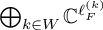 . The diagonal action of
$S^1$
. The diagonal action of
$S^1$
 on
$\bigoplus _{k\in W}{\mathbb C}^{\ell _F^{(k)}}$
on
$\bigoplus _{k\in W}{\mathbb C}^{\ell _F^{(k)}}$
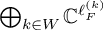 of weight
$k\in W$
of weight
$k\in W$
 on each summand
${\mathbb C}^{\ell _F^{(k)}}$
on each summand
${\mathbb C}^{\ell _F^{(k)}}$
 commutes with the action of
$K_F$
commutes with the action of
$K_F$
 , inducing an
$S^1$
, inducing an
$S^1$
 -action on the right-hand side of (3.3), which makes it an
$S^1$
-action on the right-hand side of (3.3), which makes it an
$S^1$
 -equivariant identification. Note also that the symplectic structure on
$\Sigma _F$
-equivariant identification. Note also that the symplectic structure on
$\Sigma _F$
 is induced by the standard complex structure on each
${\mathbb C}^{\ell _F^{(k)}}$
is induced by the standard complex structure on each
${\mathbb C}^{\ell _F^{(k)}}$
 via this decomposition. In what follows, we will write
$W_\pm :=\{w\in W\,|\,\pm w\in {\mathbb N}\}$
via this decomposition. In what follows, we will write
$W_\pm :=\{w\in W\,|\,\pm w\in {\mathbb N}\}$
 for the sets of positive and negative weights, respectively, so that by (3.2) there is a decomposition

where
$\Sigma _F^\pm :=\bigoplus _{k\in W_\pm }\Sigma _F^{(k)}$
 . Setting
$ \ell ^\pm _F:=\mathrm {rk}_{\mathbb C}\,\Sigma _F^\pm =\sum _{k\in W_\pm }\ell _F^{(k)} $
. Setting
$ \ell ^\pm _F:=\mathrm {rk}_{\mathbb C}\,\Sigma _F^\pm =\sum _{k\in W_\pm }\ell _F^{(k)} $
 , the decomposition (3.4) is induced by the natural embedding
$K_F\subset U(\ell ^+_F)\times U(\ell ^-_F)$
, the decomposition (3.4) is induced by the natural embedding
$K_F\subset U(\ell ^+_F)\times U(\ell ^-_F)$
 . We write
${\mathbb C}^{\ell ^\pm _F}=\bigoplus _{k\in W_\pm }{\mathbb C}^{\ell _F^{(k)}}$
. We write
${\mathbb C}^{\ell ^\pm _F}=\bigoplus _{k\in W_\pm }{\mathbb C}^{\ell _F^{(k)}}$
 and set
$\ell _F:=\mathrm {rk}_{\mathbb C}\,\Sigma _F$
and set
$\ell _F:=\mathrm {rk}_{\mathbb C}\,\Sigma _F$
 .
.
Let
$\omega _{\Sigma _F}$
 be a symplectic form on a neighborhood
$V_F$
be a symplectic form on a neighborhood
$V_F$
 of the zero section in
$\Sigma _F$
of the zero section in
$\Sigma _F$
 such that its restriction to the fibers of
$\Sigma _F$
such that its restriction to the fibers of
$\Sigma _F$
 coincides with the standard symplectic form induced by
$\omega ^{\perp }$
coincides with the standard symplectic form induced by
$\omega ^{\perp }$
 , while the restriction
$(T\Sigma _F,\omega _{\Sigma _F})|_F$
, while the restriction
$(T\Sigma _F,\omega _{\Sigma _F})|_F$
 to the zero section
$F\subset \Sigma _F$
to the zero section
$F\subset \Sigma _F$
 coincides with
$(TM,\omega )|_F$
coincides with
$(TM,\omega )|_F$
 via the natural identification of
$TM$
via the natural identification of
$TM$
 with
$T\Sigma _F$
with
$T\Sigma _F$
 over F. The next proposition gives a canonical description of the moment map
${ \mathcal J}:M\to {\mathbb R}$
over F. The next proposition gives a canonical description of the moment map
${ \mathcal J}:M\to {\mathbb R}$
 in a neighborhood of each
$F \in {\mathcal F}$
in a neighborhood of each
$F \in {\mathcal F}$
 , and constitutes the basis for the computations of the next sections. It is a straightforward consequence of the equivariant Darboux lemma, as explained for instance in [Reference Guillemin, Lerman and Sternberg13, Section 2.2].
Proposition 3.2 (Local normal form theorem)
For each
$F\in {\mathcal F}$
 there is an
$S^1$
there is an
$S^1$
 -equivariant symplectomorphism
$\Phi _F:V_F\rightarrow U_F$
-equivariant symplectomorphism
$\Phi _F:V_F\rightarrow U_F$
 from the open tubular neighborhood
$(V_F,\omega _{\Sigma _F})$
from the open tubular neighborhood
$(V_F,\omega _{\Sigma _F})$
 of the zero section in
$\Sigma _F$
of the zero section in
$\Sigma _F$
 onto an open neighborhood
$U_F\subset (M,\omega )$
onto an open neighborhood
$U_F\subset (M,\omega )$
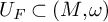 of F, such that

where
$Q_F$
 is the
$K_F$
is the
$K_F$
 -invariant quadratic form on
$\bigoplus _{k\in W}{\mathbb C}^{\ell _F^{(k)}}$
-invariant quadratic form on
$\bigoplus _{k\in W}{\mathbb C}^{\ell _F^{(k)}}$
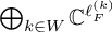 defined by

We write

for the submanifold formed fiberwise by the smooth points of the
$0$
 -level set of the quadratic form
$Q_F$
-level set of the quadratic form
$Q_F$
 . Recalling the stratification (1.7), the set
$Z_F$
. Recalling the stratification (1.7), the set
$Z_F$
 then corresponds to the regular stratum of
$J^{-1}(\{0\})$
then corresponds to the regular stratum of
$J^{-1}(\{0\})$
 in the local normal coordinates of Proposition 3.2, since

3.2 Local model
In this section, we introduce for each
$F\in {\mathcal F}$
 coordinates on
$\bigoplus _{k\in W}{\mathbb C}^{\ell _F^{(k)}}$
coordinates on
$\bigoplus _{k\in W}{\mathbb C}^{\ell _F^{(k)}}$
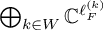 with respect to the zero level set of the quadric
$Q_F$
with respect to the zero level set of the quadric
$Q_F$
 , which will be extended in Section 3.3 to the symplectic normal bundle using the framework of the previous section. We will consider
$\bigoplus _{k\in W}{\mathbb C}^{\ell _F^{(k)}}$
, which will be extended in Section 3.3 to the symplectic normal bundle using the framework of the previous section. We will consider
$\bigoplus _{k\in W}{\mathbb C}^{\ell _F^{(k)}}$
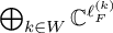 as equipped with the diagonal
$S^1$
as equipped with the diagonal
$S^1$
 -action of weight
$k\in W$
-action of weight
$k\in W$
 on each summand
${\mathbb C}^{\ell _F^{(k)}}$
on each summand
${\mathbb C}^{\ell _F^{(k)}}$
 . To begin, we define the sets

Further, for any
$k_0\in W$
 we write

for the canonical projection, and introduce the weighted Euclidean norms

We then introduce the ellipsoids

Note that the norms
$\left \| \cdot \right \|_{F\pm }$
 are both
$S^1$
are both
$S^1$
 - and
$K_F$
- and
$K_F$
 -invariant. The quadratic form
$Q_F$
-invariant. The quadratic form
$Q_F$
 from (3.5) can be written in norm notation as

Later, it will also be convenient to consider the weighted Hermitian norm

Next, for each weight
$k\in W$
 , we introduce the following standard symplectic and angular forms over
${\mathbb C}^{\ell _F^{(k)}}$
, we introduce the following standard symplectic and angular forms over
${\mathbb C}^{\ell _F^{(k)}}$
 for any
$w=(w_1'+iw_1",\cdots , w_{\ell _F^{(k)}}'+iw_{\ell _F^{(k)}}") \in {\mathbb C}^{\ell _F^{(k)}}$
for any
$w=(w_1'+iw_1",\cdots , w_{\ell _F^{(k)}}'+iw_{\ell _F^{(k)}}") \in {\mathbb C}^{\ell _F^{(k)}}$
 by setting

They are related by
$\omega _{(k)}=\frac {1}{2}d\alpha _{(k)}$
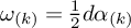 . For any
$X\in \mathbf {\mathfrak g}$
. For any
$X\in \mathbf {\mathfrak g}$
 inducing the fundamental vector field
$\tilde X\in \mathrm {C^{\infty }}({\mathbb C}^{\ell _F^{(k)}},T{\mathbb C}^{\ell _F^{(k)}})$
inducing the fundamental vector field
$\tilde X\in \mathrm {C^{\infty }}({\mathbb C}^{\ell _F^{(k)}},T{\mathbb C}^{\ell _F^{(k)}})$
 associated with the
$S^1$
associated with the
$S^1$
 -action on
${\mathbb C}^{\ell _F^{(k)}}$
-action on
${\mathbb C}^{\ell _F^{(k)}}$
 of weight
$k\in W$
of weight
$k\in W$
 we then get

where
$x\in {\mathbb R}$
 is the image of
$X\in \mathbf {\mathfrak g}$
is the image of
$X\in \mathbf {\mathfrak g}$
 via the identification (2.6). If we now introduce the
$1$
via the identification (2.6). If we now introduce the
$1$
 -forms

then (3.13) and (3.9) imply that the
$1$
 -forms defined by


are connection forms in the sense of Formula (2.8) for the diagonal
$S^1$
 -action of weight
$k\in W$
-action of weight
$k\in W$
 on the k-th summand on
${\mathbb C}^{\ell _F^\pm }_{\bullet }$
on the k-th summand on
${\mathbb C}^{\ell _F^\pm }_{\bullet }$
 and
${\mathbb C}^{\ell _F^+,\ell _F^-}_{\bullet \bullet }$
and
${\mathbb C}^{\ell _F^+,\ell _F^-}_{\bullet \bullet }$
 respectively defined in (3.8).
The following simple lemma will be crucial for all our local and global considerations. Recall the general notation for inclusions and projections introduced at the beginning of Section 2.
Lemma 3.3. Let
$S\subset \bigoplus _{k\in W}{\mathbb C}^{\ell _F^{(k)}}$
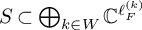 be an embedded smooth submanifold,
$f:(0,\infty )\to (0,\infty )$
be an embedded smooth submanifold,
$f:(0,\infty )\to (0,\infty )$
 a smooth function, and consider the smooth map
$\Psi _{S,f}:S\times (0,\infty )\to \bigoplus _{k\in W}{\mathbb C}^{\ell _F^{(k)}}$
a smooth function, and consider the smooth map
$\Psi _{S,f}:S\times (0,\infty )\to \bigoplus _{k\in W}{\mathbb C}^{\ell _F^{(k)}}$
 ,
$(w,r)\mapsto f(r)w$
,
$(w,r)\mapsto f(r)w$
 . Then one has for each
$k\in W$
. Then one has for each
$k\in W$


Proof. Let
$v\in T_{y}(S \times (0,\infty ))$
 be a tangent vector at
$y:=(w, r)\in S \times (0,\infty )$
be a tangent vector at
$y:=(w, r)\in S \times (0,\infty )$
 and
$\gamma _v(t)=(w(t), r(t))$
and
$\gamma _v(t)=(w(t), r(t))$
 a smooth curve with
$\dot \gamma _v(0)=v$
a smooth curve with
$\dot \gamma _v(0)=v$
 ,
$\gamma _v(0)=y$
,
$\gamma _v(0)=y$
 . Identifying
$T_{y}(S \times (0,\infty ))$
. Identifying
$T_{y}(S \times (0,\infty ))$
 with a subspace of
$\bigoplus _{k\in W}{\mathbb C}^{\ell _F^{(k)}}\times {\mathbb R}$
with a subspace of
$\bigoplus _{k\in W}{\mathbb C}^{\ell _F^{(k)}}\times {\mathbb R}$
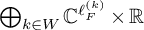 we get

so that with the identification
$w_j\equiv w_j' \operatorname {\mathrm {\partial }}_{w_j'}+w_j" \operatorname {\mathrm {\partial }}_{w_j"}$
 in the notation of (3.12) we obtain

We will now proceed with separate treatments of the cases
$0\in \partial \,{ \mathcal J}(M)$
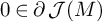 and
$0\in \operatorname {\mathrm {Int}}{ \mathcal J}(M)$
and
$0\in \operatorname {\mathrm {Int}}{ \mathcal J}(M)$
 , respectively. As explained in the introduction, in the first case
${\mathcal F}_0$
, respectively. As explained in the introduction, in the first case
${\mathcal F}_0$
 consists of only one component
$F={ \mathcal J}^{-1}(\left \{ 0 \right \})$
consists of only one component
$F={ \mathcal J}^{-1}(\left \{ 0 \right \})$
 and
$Q_F$
and
$Q_F$
 is definite, while in the second case,
$Q_F$
is definite, while in the second case,
$Q_F$
 is indefinite for all
$F\in {\mathcal F}^0$
is indefinite for all
$F\in {\mathcal F}^0$
 .
.
3.2.1 Definite case
Let us begin with the easier definite case, so that either
$\ell _F^-=0$
 or
$\ell _F^+=0$
or
$\ell _F^+=0$
 , and write
$\ell _F:=\ell _F^+>0$
, and write
$\ell _F:=\ell _F^+>0$
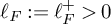 if
$F\in {\mathcal F}_+$
if
$F\in {\mathcal F}_+$
 and
$\ell _F:=\ell _F^->0$
and
$\ell _F:=\ell _F^->0$
 if
$F\in {\mathcal F}_-$
if
$F\in {\mathcal F}_-$
 . The diagonal action of
$S^1$
. The diagonal action of
$S^1$
 on
${\mathbb C}^{\ell _F}=\bigoplus _{k\in W}{\mathbb C}^{\ell _F^{(k)}}$
on
${\mathbb C}^{\ell _F}=\bigoplus _{k\in W}{\mathbb C}^{\ell _F^{(k)}}$
 considered in Section 3.1 restricts to a locally free action on
$S^{2\ell _F-1}$
considered in Section 3.1 restricts to a locally free action on
$S^{2\ell _F-1}$
 , and we introduce the connection form

as the restriction of (3.15) to
$S^{2\ell _F-1}$
 .
.
We now introduce spherical polar coordinates in
${\mathbb C}^{\ell _F}_{\bullet }$
 via the diffeomorphism

which is equivariant for the action of
$S^1$
 introduced above on the first factor and the trivial action on the second factor of
$S^{2\ell _F-1}\times (0,\infty )$
introduced above on the first factor and the trivial action on the second factor of
$S^{2\ell _F-1}\times (0,\infty )$
 . It defines on
${\mathbb C}^{\ell _F}_{\bullet }$
. It defines on
${\mathbb C}^{\ell _F}_{\bullet }$
 the radial coordinate

which is related to the quadratic form
$Q_F$
 by
by

Applying Lemma 3.3 to
$S=S^{2\ell _F-1}$
 and
$f=\mathrm {id}$
and
$f=\mathrm {id}$
 one immediately sees that

Since
$\omega _{\mathrm {std}}=\pm \frac {1}{2}d\theta $
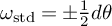 and
$\Theta =\mathrm {inc}^\ast _{S^{2\ell _F-1}}\theta $
and
$\Theta =\mathrm {inc}^\ast _{S^{2\ell _F-1}}\theta $
 , we deduce from this the useful identity

3.2.2 Indefinite case
Let us now turn to the indefinite case, so that
$\ell _F^+,\ell _F^->0$
 . Departing from the quadric formed by the zero level set of
$Q_F$
. Departing from the quadric formed by the zero level set of
$Q_F$
 we define the slit quadric

which is a smooth submanifold of the set
${\mathbb C}^{\ell _F^+,\ell _F^-}_{\bullet \bullet }$
 defined in (3.8). The diagonal action of
$S^1$
defined in (3.8). The diagonal action of
$S^1$
 on
${\mathbb C}^{\ell _F}=\bigoplus _{k\in W}{\mathbb C}^{\ell _F^{(k)}}$
on
${\mathbb C}^{\ell _F}=\bigoplus _{k\in W}{\mathbb C}^{\ell _F^{(k)}}$
 considered in Section 3.1 restricts to locally free
$S^1$
considered in Section 3.1 restricts to locally free
$S^1$
 -actions on
$\mathcal {Q}_\times \subset {\mathbb C}^{\ell _F^+,\ell _F^-}_{\bullet \bullet }$
-actions on
$\mathcal {Q}_\times \subset {\mathbb C}^{\ell _F^+,\ell _F^-}_{\bullet \bullet }$
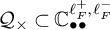 and the product of ellipsoids

of the ellipsoids (3.10). Besides the connection form (3.16) we introduce now also the
$1$
 -form
-form

on
${\mathbb C}^{\ell _F^+,\ell _F^-}_{\bullet \bullet }$
 , and introduce the corresponding restrictions

to
$S^{2\ell _F^+-1}_+\times S^{2\ell _F^--1}_-$
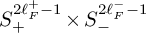 . Clearly,
$\Theta \in \Omega ^1(S^{2\ell _F^+-1}_+\times S^{2\ell _F^--1}_-,{\mathbb R})$
. Clearly,
$\Theta \in \Omega ^1(S^{2\ell _F^+-1}_+\times S^{2\ell _F^--1}_-,{\mathbb R})$
 is a connection for the
$S^1$
is a connection for the
$S^1$
 -action on
$S^{2\ell _F^+-1}_+\times S^{2\ell _F^--1}_-$
-action on
$S^{2\ell _F^+-1}_+\times S^{2\ell _F^--1}_-$
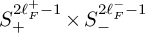 . On the other hand, the
$1$
. On the other hand, the
$1$
 -form
$\overline \Theta \in \Omega ^1(S^{2\ell _F^+-1}_+\times S^{2\ell _F^--1}_-,{\mathbb R})$
-form
$\overline \Theta \in \Omega ^1(S^{2\ell _F^+-1}_+\times S^{2\ell _F^--1}_-,{\mathbb R})$
 is basic in the sense of Proposition 2.4.
Let us now introduce polar moment coordinates in
${\mathbb C}^{\ell _F^+,\ell _F^-}_{\bullet \bullet }$
 via the diffeomorphism

The map
$\Psi $
 is at the basis of our local model. It is equivariant under the action of
$S^1$
is at the basis of our local model. It is equivariant under the action of
$S^1$
 introduced above on
$S^{2\ell _F^+-1}_+\times S^{2\ell _F^--1}_-$
introduced above on
$S^{2\ell _F^+-1}_+\times S^{2\ell _F^--1}_-$
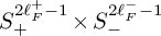 and the trivial action on
$(0,\infty )\times {\mathbb R} $
and the trivial action on
$(0,\infty )\times {\mathbb R} $
 , and defines for
$w \in {\mathbb C}^{\ell _F^+,\ell _F^-}_{\bullet \bullet }$
, and defines for
$w \in {\mathbb C}^{\ell _F^+,\ell _F^-}_{\bullet \bullet }$
 the coordinates

The slit quadric
$\mathcal {Q}_\times \subset {\mathbb C}^{\ell _F^+,\ell _F^-}_{\bullet \bullet }$
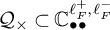 defined in (3.22) corresponds to the set
$\{q=0\}$
defined in (3.22) corresponds to the set
$\{q=0\}$
 , while the coordinate r is radial on
${\mathcal {Q}_\times }$
, while the coordinate r is radial on
${\mathcal {Q}_\times }$
 . Moreover, composing the retraction

with
$\Psi $
 gives us an
$S^1$
gives us an
$S^1$
 -equivariant surjection

Let
$\mathrm {pr}_{S^{2\ell _F^+-1}_+\times S^{2\ell _F^--1}_-}:S^{2\ell _F^+-1}_+\times S^{2\ell _F^--1}_-\times (0,\infty )\times {\mathbb R}\longrightarrow S^{2\ell _F^+-1}_+\times S^{2\ell _F^--1}_-$
 be the canonical projection. We then have
Lemma 3.4. Write
$\alpha :=\frac 12 (\alpha ^++\alpha ^-)$
 and
$\overline \alpha :=\frac 12 (\alpha ^+-\alpha ^-)$
and
$\overline \alpha :=\frac 12 (\alpha ^+-\alpha ^-)$
 . In the coordinates (3.27), one has

Proof. Consider
$\Psi $
 and
$\mathrm {pr}_{S^{2\ell _F^+-1}_+\times S^{2\ell _F^--1}_-}$
and
$\mathrm {pr}_{S^{2\ell _F^+-1}_+\times S^{2\ell _F^--1}_-}$
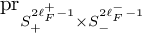 as families of maps defined on
$S^{2\ell _F^+-1}_+\times S^{2\ell _F^--1}_-\times (0,\infty )$
as families of maps defined on
$S^{2\ell _F^+-1}_+\times S^{2\ell _F^--1}_-\times (0,\infty )$
 and parametrized by
$q\in {\mathbb R}$
and parametrized by
$q\in {\mathbb R}$
 . Defining
$f_q^\pm :(0,\infty )\to (0,\infty )$
. Defining
$f_q^\pm :(0,\infty )\to (0,\infty )$
 by
$f_q^\pm (r):=\sqrt {\sqrt {r^4+q^2}\pm q}$
by
$f_q^\pm (r):=\sqrt {\sqrt {r^4+q^2}\pm q}$
 , we can apply Lemma 3.3 with
$S=S^{2\ell _F^+-1}_+\times S^{2\ell _F^--1}_-$
, we can apply Lemma 3.3 with
$S=S^{2\ell _F^+-1}_+\times S^{2\ell _F^--1}_-$
 and
$f=f_q^\pm $
and
$f=f_q^\pm $
 to get

concluding the proof.
A direct consequence of Lemma 3.4 is the following indefinite version of (3.21).
Corollary 3.5. In the coordinates (3.26) one has

Proof. As
$\omega _{\mathrm {std}}=d\bar \alpha $
 , we apply d on both sides of the equation in Lemma 3.4 involving
$\bar \alpha $
, we apply d on both sides of the equation in Lemma 3.4 involving
$\bar \alpha $
 , yielding

We now assert that

Indeed, since
$\overline \Theta =\mathrm {inc}^\ast _{S^{2\ell _F^+-1}_+\times S^{2\ell _F^--1}_-}\bar \alpha $
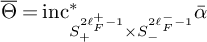 , this is a consequence of the relation

which follows from Lemma 3.3 applied with
$S=S^{2\ell _F^+-1}_+\times S^{2\ell _F^--1}_-$
 ,
$f=\mathrm {id}$
,
$f=\mathrm {id}$
 , and
$q\in {\mathbb R}$
, and
$q\in {\mathbb R}$
 as an additional parameter.
3.3 Application to the symplectic normal bundle
We now translate the fiberwise considerations from Section 3.2 into global statements on the symplectic normal bundle
$\Sigma _F$
 , identified with the associated bundle
$P_F\times _{K_F}\bigoplus _{k\in W}{\mathbb C}^{\ell _F^{(k)}}$
, identified with the associated bundle
$P_F\times _{K_F}\bigoplus _{k\in W}{\mathbb C}^{\ell _F^{(k)}}$
 as in (3.3).
Choose a
$K_F$
 -connection on the principal bundle
$\nu _{P_F}:P_F \rightarrow F$
-connection on the principal bundle
$\nu _{P_F}:P_F \rightarrow F$
 , inducing a Hermitian connection
$\nabla ^{\Sigma _F}$
, inducing a Hermitian connection
$\nabla ^{\Sigma _F}$
 on
$\Sigma _F$
on
$\Sigma _F$
 that preserves the decomposition (3.2). This provides us with a splitting of the short exact sequence

of vector bundles over
$\Sigma _F$
 , yielding the global decomposition

where
$T^{\mathrm {hor}}F\simeq \nu _{\Sigma _F}^*TF$
 is the horizontal distribution defined by
$\nabla ^{\Sigma _F}$
is the horizontal distribution defined by
$\nabla ^{\Sigma _F}$
 and
$\nu _{\Sigma _F}^*\Sigma _F\subset T\Sigma _F$
and
$\nu _{\Sigma _F}^*\Sigma _F\subset T\Sigma _F$
 is the vertical tangent bundle to the fibers. Choose a compatible almost complex structure
$J_F\in \operatorname {\mathrm {End}}(TF)$
is the vertical tangent bundle to the fibers. Choose a compatible almost complex structure
$J_F\in \operatorname {\mathrm {End}}(TF)$
 over
$(F,\omega _F)$
over
$(F,\omega _F)$
 . Together with the natural complex structure
$J_{\Sigma _F}\in \operatorname {\mathrm {End}}(\Sigma _F)$
. Together with the natural complex structure
$J_{\Sigma _F}\in \operatorname {\mathrm {End}}(\Sigma _F)$
 , this induces via the decomposition (3.31) an
$S^1$
, this induces via the decomposition (3.31) an
$S^1$
 -invariant almost complex structure
$J\in \operatorname {\mathrm {End}}(T\Sigma _F)$
-invariant almost complex structure
$J\in \operatorname {\mathrm {End}}(T\Sigma _F)$
 over the total space of
$\Sigma _F$
over the total space of
$\Sigma _F$
 .
.
For any
$k_0\in W$
 , we define
$f_{k_0}\in \mathrm {C^{\infty }}(\Sigma _F,{\mathbb R})$
, we define
$f_{k_0}\in \mathrm {C^{\infty }}(\Sigma _F,{\mathbb R})$
 by setting

where
$\left \| \cdot \right \|$
 denotes the standard Hermitian norm. Note that
$f_{k_0}$
denotes the standard Hermitian norm. Note that
$f_{k_0}$
 is well-defined since for each
$k\in W$
is well-defined since for each
$k\in W$
 the structure group
$K_F$
the structure group
$K_F$
 acts by
$\mathrm {U}(\ell _F^{(k)})$
acts by
$\mathrm {U}(\ell _F^{(k)})$
 on
${\mathbb C}^{\ell _F^{(k)}}$
on
${\mathbb C}^{\ell _F^{(k)}}$
 and thus preserves the Hermitian norm. Using this, we define the
$1$
and thus preserves the Hermitian norm. Using this, we define the
$1$
 -form
$\alpha _{k_0}\in \Omega ^1(\Sigma _F,{\mathbb R})$
-form
$\alpha _{k_0}\in \Omega ^1(\Sigma _F,{\mathbb R})$
 by
by

Comparing with (3.12), one readily checks that for any
$p\in F$
 the restriction of
$\alpha _{k_0}\in \Omega ^1(\Sigma _F,{\mathbb R})$
the restriction of
$\alpha _{k_0}\in \Omega ^1(\Sigma _F,{\mathbb R})$
 to the fiber
$(\Sigma _F)_p\subset \Sigma _F$
to the fiber
$(\Sigma _F)_p\subset \Sigma _F$
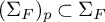 , seen as a submanifold in the total space of
$\Sigma _F$
, seen as a submanifold in the total space of
$\Sigma _F$
 , satisfies

in any trivialization
$(\Sigma _F)_p\simeq \bigoplus _{k\in W}{\mathbb C}^{\ell _F^{(k)}}$
 compatible with the
$K_F$
compatible with the
$K_F$
 -principal bundle structure (3.3). Following (3.14), (3.15) and (3.16), we write

so that the
$1$
 -forms given by


define connections for the
$S^1$
 -action on
$P_F\times _{K_F}{\mathbb C}^{\ell _F^\pm }_{\bullet }$
-action on
$P_F\times _{K_F}{\mathbb C}^{\ell _F^\pm }_{\bullet }$
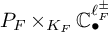 and
$P_F\times _{K_F}{\mathbb C}^{\ell _F^+,\ell _F^-}_{\bullet \bullet }$
and
$P_F\times _{K_F}{\mathbb C}^{\ell _F^+,\ell _F^-}_{\bullet \bullet }$
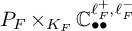 , respectively, such that for all
$p\in F$
, respectively, such that for all
$p\in F$
 the restriction of
$\theta _F^\pm ,\,\theta _F$
the restriction of
$\theta _F^\pm ,\,\theta _F$
 to the fiber over p coincides with
$\theta ^\pm ,\,\theta $
to the fiber over p coincides with
$\theta ^\pm ,\,\theta $
 in any trivialization
$(\Sigma _F)_p\simeq \bigoplus _{k\in W}{\mathbb C}^{\ell _F^{(k)}}$
in any trivialization
$(\Sigma _F)_p\simeq \bigoplus _{k\in W}{\mathbb C}^{\ell _F^{(k)}}$
 compatible with the
$K_F$
compatible with the
$K_F$
 -principal bundle structure (3.3). We also define the vertical form
$\omega _{\mathrm {vert}}\in \Omega ^2(\Sigma _F,{\mathbb R})$
-principal bundle structure (3.3). We also define the vertical form
$\omega _{\mathrm {vert}}\in \Omega ^2(\Sigma _F,{\mathbb R})$
 by
by

Comparing with (3.12) and (3.34), for all
$p\in F$
 the restriction of
$\omega _{\mathrm {vert}}\in \Omega ^2(\Sigma _F,{\mathbb R})$
the restriction of
$\omega _{\mathrm {vert}}\in \Omega ^2(\Sigma _F,{\mathbb R})$
 to the fiber
$(\Sigma _F)_p\subset \Sigma _F$
to the fiber
$(\Sigma _F)_p\subset \Sigma _F$
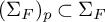 satisfies

in any trivialization
$(\Sigma _F)_p\simeq \bigoplus _{k\in W}{\mathbb C}^{\ell _F^{(k)}}$
 compatible with the
$K_F$
compatible with the
$K_F$
 -principal bundle structure (3.3), where
$\omega _{\mathrm {std}}$
-principal bundle structure (3.3), where
$\omega _{\mathrm {std}}$
 is the standard symplectic form on
$\bigoplus _{k\in W}{\mathbb C}^{\ell _F^{(k)}}$
is the standard symplectic form on
$\bigoplus _{k\in W}{\mathbb C}^{\ell _F^{(k)}}$
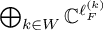 induced by (3.12) for each
$k\in W$
induced by (3.12) for each
$k\in W$
 . Furthermore, note that the restriction
$T\Sigma _F|_F$
. Furthermore, note that the restriction
$T\Sigma _F|_F$
 over the zero section
$F\subset \Sigma _F$
over the zero section
$F\subset \Sigma _F$
 naturally identifies with the restriction
$TM|_F$
naturally identifies with the restriction
$TM|_F$
 over
$F\subset M$
over
$F\subset M$
 , and the restriction of
$\omega _{\mathrm {vert}}$
, and the restriction of
$\omega _{\mathrm {vert}}$
 to
$T\Sigma _F|_F$
to
$T\Sigma _F|_F$
 coincides with
$\omega ^{\perp }$
coincides with
$\omega ^{\perp }$
 in the decomposition (3.1). Consequently, we can explicitly choose the symplectic form
$\omega _{\Sigma _F}$
in the decomposition (3.1). Consequently, we can explicitly choose the symplectic form
$\omega _{\Sigma _F}$
 from Proposition 3.2 to be given by

By construction, the almost complex structure
$J\in \operatorname {\mathrm {End}}(T\Sigma _F)$
 over
$\Sigma _F$
over
$\Sigma _F$
 is compatible with
$\omega _{\Sigma _F}$
is compatible with
$\omega _{\Sigma _F}$
 , and we write
$g^{T\Sigma _F}:=\omega _{\Sigma _F}(\cdot ,J\cdot )$
, and we write
$g^{T\Sigma _F}:=\omega _{\Sigma _F}(\cdot ,J\cdot )$
 for the induced
$S^1$
for the induced
$S^1$
 -invariant Riemannian metric over
$V_F$
-invariant Riemannian metric over
$V_F$
 .
.
3.3.1 Definite case
Let
$F\in {\mathcal F}$
 be such that
$Q_F$
be such that
$Q_F$
 is definite. Recall the definition of
$\ell _F$
is definite. Recall the definition of
$\ell _F$
 from the beginning of Section 3.2.1. As the linear action of
$K_F$
from the beginning of Section 3.2.1. As the linear action of
$K_F$
 on
${\mathbb C}^{\ell _F}$
on
${\mathbb C}^{\ell _F}$
 preserves
$S^{2\ell _F-1}$
preserves
$S^{2\ell _F-1}$
 , we can consider the associated sphere bundle
$ S_F:= P_F\times _{K_F}S^{2\ell _F-1} $
, we can consider the associated sphere bundle
$ S_F:= P_F\times _{K_F}S^{2\ell _F-1} $
 inside
$\Sigma _F=P_F\times _{K_F}{\mathbb C}^{\ell _F}$
inside
$\Sigma _F=P_F\times _{K_F}{\mathbb C}^{\ell _F}$
 , with bundle projection
$\nu _{S_F}:S_F\to F$
, with bundle projection
$\nu _{S_F}:S_F\to F$
 . The
$S^1$
. The
$S^1$
 -action on
$\Sigma _F$
-action on
$\Sigma _F$
 restricts to a locally free
$S^1$
restricts to a locally free
$S^1$
 -action on
$S_F$
-action on
$S_F$
 for which we have the connection

given by restriction of the connection
$\theta _F$
 from (3.36). Using (3.8) to define the subbundle

the
$S^1$
 -equivariant diffeomorphism
$\Psi $
-equivariant diffeomorphism
$\Psi $
 from (3.18) globalizes to an
$S^1$
from (3.18) globalizes to an
$S^1$
 -equivariant diffeomorphism

where
$S^1$
 acts on
$S_F\times (0,\infty )$
acts on
$S_F\times (0,\infty )$
 by the product of the
$S^1$
by the product of the
$S^1$
 -action on
$S_F$
-action on
$S_F$
 and the trivial action on
$(0,\infty )$
and the trivial action on
$(0,\infty )$
 .
$\Psi _{F}$
.
$\Psi _{F}$
 promotes the coordinate r from (3.19) to a global fiber-radial coordinate r on the bundle
$\Sigma _{F\bullet }$
promotes the coordinate r from (3.19) to a global fiber-radial coordinate r on the bundle
$\Sigma _{F\bullet }$
 . Its relation to
$Q_F$
. Its relation to
$Q_F$
 is given by (3.20) with
${\mathbb C}^{\ell _F}_{\bullet }$
is given by (3.20) with
${\mathbb C}^{\ell _F}_{\bullet }$
 replaced by
$\Sigma _{F\bullet }$
replaced by
$\Sigma _{F\bullet }$
 . Note that
$S_F\times (0,\infty )$
. Note that
$S_F\times (0,\infty )$
 is a fiber bundle over F with the projection
$\nu _{S_F\times (0,\infty )}:=\nu _{S_F}\circ \mathrm {pr}_{S_F}$
is a fiber bundle over F with the projection
$\nu _{S_F\times (0,\infty )}:=\nu _{S_F}\circ \mathrm {pr}_{S_F}$
 . We state the global version of (3.21) in
Corollary 3.6. In the coordinate (3.19) provided by the diffeomorphism (3.42) we have

Proof. In view of the definition (3.41) of
$\Theta _{S_F}$
 and the definition (3.42) of
$\Psi _{F}$
and the definition (3.42) of
$\Psi _{F}$
 the assertion follows from (3.40), (3.21), and (3.39).
For a better overview, we illustrate the maps appearing in Corollary 3.6 in the diagram

in which everything commutes except the triangle formed by
$\mathrm {pr}_{S_F}$
 ,
$\mathrm {inc}_{S_F}$
,
$\mathrm {inc}_{S_F}$
 , and
$\Psi _{F}$
, and
$\Psi _{F}$
 , which commutes only up to
$S^1$
, which commutes only up to
$S^1$
 -equivariant homotopy.
3.3.2 Indefinite case
Let
$F\in {\mathcal F}$
 be such that
$Q_F$
be such that
$Q_F$
 is indefinite. As the linear action of
$K_F$
is indefinite. As the linear action of
$K_F$
 on
${\mathbb C}^{\ell _F^++\ell _F^-}$
on
${\mathbb C}^{\ell _F^++\ell _F^-}$
 preserves the bi-ellipsoid (3.23), we can consider the associated fiber bundle

inside
$\Sigma _F\cong P_F\times _{K_F}{\mathbb C}^{\ell _F^++\ell _F^-}$
 . Furthermore, the
$0$
. Furthermore, the
$0$
 -level set
$Z_F\subset \Sigma _F\setminus F$
-level set
$Z_F\subset \Sigma _F\setminus F$
 defined in (3.6) has the fiber bundle structure

associated with the slit quadric (3.22). Recall that we write
$\nu _{S_F}:S_F\to F$
 and
$\nu _{Z_F}:Z_F\to F$
and
$\nu _{Z_F}:Z_F\to F$
 for the fiber bundle projections. The action of
$S^1$
for the fiber bundle projections. The action of
$S^1$
 on
$\Sigma _F$
on
$\Sigma _F$
 restricts to locally free
$S^1$
restricts to locally free
$S^1$
 -actions on
$S_F$
-actions on
$S_F$
 and
$Z_F$
and
$Z_F$
 , respectively, and we set

where
$\theta _F$
 is the connection form on
$\Sigma _F\setminus F$
is the connection form on
$\Sigma _F\setminus F$
 from (3.37) and the
$1$
from (3.37) and the
$1$
 -forms
$\alpha _k$
-forms
$\alpha _k$
 were defined in (3.33). Thus,
$\Theta _{S_F}$
were defined in (3.33). Thus,
$\Theta _{S_F}$
 and
$\Theta _{Z_F}$
and
$\Theta _{Z_F}$
 are connections for the
$S^1$
are connections for the
$S^1$
 -actions on
$S_F$
-actions on
$S_F$
 and
$Z_F$
and
$Z_F$
 , respectively. On the other hand,
$\overline \Theta _{S_F}$
, respectively. On the other hand,
$\overline \Theta _{S_F}$
 and
$\overline \Theta _{Z_F}$
and
$\overline \Theta _{Z_F}$
 are basic differential forms in the sense of Proposition 2.4. Using (3.8) to define the subbundle

the
$S^1$
 -equivariant diffeomorphism
$\Psi $
-equivariant diffeomorphism
$\Psi $
 from (3.26) globalizes to an
$S^1$
from (3.26) globalizes to an
$S^1$
 -equivariant diffeomorphism

where
$S^1$
 acts on
$S_F\times (0,\infty )\times {\mathbb R}$
acts on
$S_F\times (0,\infty )\times {\mathbb R}$
 by the product of the
$S^1$
by the product of the
$S^1$
 -action on
$S_F$
-action on
$S_F$
 and the trivial action on
$(0,\infty )\times {\mathbb R}$
and the trivial action on
$(0,\infty )\times {\mathbb R}$
 . The map
$\Psi _{F}$
. The map
$\Psi _{F}$
 defines coordinates (3.27) on
$\Sigma _{F\bullet \bullet }$
defines coordinates (3.27) on
$\Sigma _{F\bullet \bullet }$
 , in which
$Z_F$
, in which
$Z_F$
 coincides with
$\{q=0\}$
coincides with
$\{q=0\}$
 . The retraction
$\mathrm {ret}_{\mathcal {Q}_\times }$
. The retraction
$\mathrm {ret}_{\mathcal {Q}_\times }$
 from (3.28) and the surjection
$\pi _{\mathcal {Q}_\times }$
from (3.28) and the surjection
$\pi _{\mathcal {Q}_\times }$
 from (3.29) globalize to an
$S^1$
from (3.29) globalize to an
$S^1$
 -equivariant retraction and an
$S^1$
-equivariant retraction and an
$S^1$
 -equivariant surjection onto
$Z_F$
-equivariant surjection onto
$Z_F$
 , respectively, by defining

as well as

The restricted diffeomorphism

denoted again just by
$\Psi _F$
 for simplicity, provides the radial coordinate r on
$Z_F$
for simplicity, provides the radial coordinate r on
$Z_F$
 . Note that the space
$S_F\times (0,\infty )$
. Note that the space
$S_F\times (0,\infty )$
 , which we identify canonically with
$S_F\times (0,\infty )\times \{0\}$
, which we identify canonically with
$S_F\times (0,\infty )\times \{0\}$
 , as well as the space
$S_F\times (0,\infty )\times {\mathbb R}$
, as well as the space
$S_F\times (0,\infty )\times {\mathbb R}$
 , are fiber bundles over F with the corresponding projections
$\nu _{S_F\times (0,\infty )}$
, are fiber bundles over F with the corresponding projections
$\nu _{S_F\times (0,\infty )}$
 ,
$\nu _{S_F\times (0,\infty )\times {\mathbb R}}$
,
$\nu _{S_F\times (0,\infty )\times {\mathbb R}}$
 given by the composition of
$\nu _{S_F}$
given by the composition of
$\nu _{S_F}$
 with the canonical projections onto
$S_F$
with the canonical projections onto
$S_F$
 , respectively. These constructions lead us to the following
Corollary 3.7. In the coordinates (3.27) defined by the diffeomorphism (3.47) one has

as well as

Proof. By the definition of
$\omega _{\Sigma _F}$
 in (3.40) and (3.39), of
$\Theta _{Z_F}$
in (3.40) and (3.39), of
$\Theta _{Z_F}$
 in (3.46), and of
$\omega _{\Sigma _F}$
in (3.46), and of
$\omega _{\Sigma _F}$
 ,
$\omega _{\mathrm {vert}}$
,
$\omega _{\mathrm {vert}}$
 in (3.40) and (3.38), respectively, the claims are direct consequences of Lemma 3.4 and Corollary 3.5.
For an overview, the maps introduced above, and in particular those involved in Corollary 3.7, are illustrated in the diagram

This is the indefinite version of (3.43). In the diagram, everything commutes except the triangles involving an inclusion followed by the retraction
$\mathrm {ret}_{Z_F}$
 , a projection, or the surjection
$\pi _{Z_F}$
, a projection, or the surjection
$\pi _{Z_F}$
 , which commute only up to
$S^1$
, which commute only up to
$S^1$
 -equivariant homotopy. Note that the two canonical projections onto
$S_F$
-equivariant homotopy. Note that the two canonical projections onto
$S_F$
 are both denoted by
$\mathrm {pr}_{S_F}$
are both denoted by
$\mathrm {pr}_{S_F}$
 , whereas each fiber bundle projection onto F has its own name.
4 Kirwan maps
In the setting of Section 2.1, let
$(M,\omega ,{ \mathcal J})$
 be a Hamiltonian
$S^1$
be a Hamiltonian
$S^1$
 -manifold such that the restriction of the
$S^1$
-manifold such that the restriction of the
$S^1$
 -action to
${ \mathcal J}^{-1}(\{0\})$
-action to
${ \mathcal J}^{-1}(\{0\})$
 is locally free, and write
$\text {inc}_0:{ \mathcal J}^{-1}(\{0\})\to M$
is locally free, and write
$\text {inc}_0:{ \mathcal J}^{-1}(\{0\})\to M$
 for the inclusion map. The following classical notion goes back to Kirwan [Reference Kirwan20], which we introduce here only for
$G=S^1$
for the inclusion map. The following classical notion goes back to Kirwan [Reference Kirwan20], which we introduce here only for
$G=S^1$
 .
.
Proposition 4.1. [Reference Kalkman19, (18)] Assume that
$S^1$
 acts locally freely on the level set
${ \mathcal J}^{-1}(\{0\})\subset M$
acts locally freely on the level set
${ \mathcal J}^{-1}(\{0\})\subset M$
 , and let
$\Theta \in \Omega ^1({ \mathcal J}^{-1}(\{0\}),{\mathbb R})$
, and let
$\Theta \in \Omega ^1({ \mathcal J}^{-1}(\{0\}),{\mathbb R})$
 be a connection for the
$S^1$
be a connection for the
$S^1$
 -action. Then, for any
$\varrho (x)\in \Omega _{S^1}^*(M)$
-action. Then, for any
$\varrho (x)\in \Omega _{S^1}^*(M)$


defines a map of complexes
$\kappa :(\Omega _{S^1}^*(M),d_{\mathbf {\mathfrak g}})\to (\Omega ({ \mathcal J}^{-1}(\{0\}))^{S^1}_{\mathrm {bas}},d)$
 , inducing via the isomorphism of Proposition 2.4 a morphism

which does not depend on the choice of the connection
$\Theta \in \Omega ^1({ \mathcal J}^{-1}(\{0\}),{\mathbb R})$
 . The morphism
$\kappa $
. The morphism
$\kappa $
 is called the Kirwan map.
The notation
$\text {inc}_0^*\,\varrho (\frac {i}{2\pi }d\Theta )\in \Omega ^*({ \mathcal J}^{-1}(\{0\}),{\mathbb R})$
 means that we substitute
$\frac {i}{2\pi }d\Theta $
means that we substitute
$\frac {i}{2\pi }d\Theta $
 for X in
$\text {inc}_0^*\,\varrho (X)$
for X in
$\text {inc}_0^*\,\varrho (X)$
 , taking the wedge product with the coefficients of the power series
$\text {inc}_0^*\,\varrho (X)$
, taking the wedge product with the coefficients of the power series
$\text {inc}_0^*\,\varrho (X)$
 .
.
4.1 Regular Kirwan map of a singular symplectic quotient
Let now
$(M,\omega ,{ \mathcal J})$
 be a general Hamiltonian
$S^1$
be a general Hamiltonian
$S^1$
 -manifold, so that the symplectic quotient (1.1) is only a stratified space, and assume that
$0\in \partial \,{ \mathcal J}(M)$
-manifold, so that the symplectic quotient (1.1) is only a stratified space, and assume that
$0\in \partial \,{ \mathcal J}(M)$
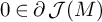 . To introduce the regular Kirwan maps appearing in Theorem 1.1, we will need the following definition.
Definition 4.2. A connection
$\Theta \in \Omega ^1({ \mathcal J}^{-1}(\{0\})^{\mathrm {reg}},{\mathbb R})$
 for the
$S^1$
for the
$S^1$
 -action on
${ \mathcal J}^{-1}(\{0\})^{\mathrm {reg}}$
-action on
${ \mathcal J}^{-1}(\{0\})^{\mathrm {reg}}$
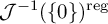 is said to have normal form near the singularities if for each
$F\in {\mathcal F}^0$
is said to have normal form near the singularities if for each
$F\in {\mathcal F}^0$
 one has

where
$U_F\subset M$
 is a neighborhood of F as in Proposition 3.2 and
$\Theta _{Z_F}\in \Omega ^1(Z_F,{\mathbb R})$
is a neighborhood of F as in Proposition 3.2 and
$\Theta _{Z_F}\in \Omega ^1(Z_F,{\mathbb R})$
 denotes the connection form (3.46) over
$Z_F\subset \Sigma _F$
denotes the connection form (3.46) over
$Z_F\subset \Sigma _F$
 via (3.7).
Using a partition of unity, one readily constructs a connection with normal form near all
$F\in {\mathcal F}^0$
 .
.
Definition 4.3. The regular Kirwan map is the map of complexes

defined by the restriction of the formula (4.1) to the regular stratum
${ \mathcal J}^{-1}(\{0\})^{\mathrm {reg}}$
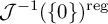 of the stratification (1.7) and using a connection
$\Theta \in \Omega ^1({ \mathcal J}^{-1}(\{0\})^{\mathrm {reg}},{\mathbb R})$
of the stratification (1.7) and using a connection
$\Theta \in \Omega ^1({ \mathcal J}^{-1}(\{0\})^{\mathrm {reg}},{\mathbb R})$
 with normal form near the singularities in the sense of Definition 4.2.
The regular Kirwan map of Definition 4.3 appears in the regular term of the Hirzebruch-Riemann-Roch type formula of Theorem 1.1 inside an integral over the non-compact manifold
${\mathscr M}_0^{\mathrm {reg}}$
 , which is naturally oriented by its symplectic volume form. The next Lemma shows that this integral in fact converges.
Lemma 4.4. For all
$\varrho \in \Omega _{S^1}^*(M)$
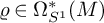 and
$m\in {\mathbb N}$
and
$m\in {\mathbb N}$
 , the integral

converges, where
$\{U_j\}_{j\in {\mathbb N}}$
 denotes an arbitrary exhaustion of
${\mathscr M}_0^{\mathrm {reg}}$
denotes an arbitrary exhaustion of
${\mathscr M}_0^{\mathrm {reg}}$
 by relatively compact open sets, and does not depend on the choice of the exhaustion.
Proof. For any
$F\in {\mathcal F}^0$
 , recall from (3.7) that the diffeomorphism
$\Phi _F$
, recall from (3.7) that the diffeomorphism
$\Phi _F$
 of the local normal form of Proposition 3.2 sends
$Z_F\cap V_F$
of the local normal form of Proposition 3.2 sends
$Z_F\cap V_F$
 to
${ \mathcal J}^{-1}(\{0\})^{\mathrm {reg}}\cap U_F$
to
${ \mathcal J}^{-1}(\{0\})^{\mathrm {reg}}\cap U_F$
 , where
$Z_F=Q_F^{-1}(\{0\})\setminus F$
, where
$Z_F=Q_F^{-1}(\{0\})\setminus F$
 has been introduced in Equation (3.6). Keeping in mind the coordinates (3.27), for any small enough
$\varepsilon>0$
has been introduced in Equation (3.6). Keeping in mind the coordinates (3.27), for any small enough
$\varepsilon>0$
 let
$B_{F,\varepsilon }\subset { \mathcal J}^{-1}(\{0\})\cap U_F$
let
$B_{F,\varepsilon }\subset { \mathcal J}^{-1}(\{0\})\cap U_F$
 be the neighborhood of F defined by

Let
$\Theta \in \Omega ^1({ \mathcal J}^{-1}(\{0\})^{\mathrm {reg}},{\mathbb R})$
 be a connection of normal form near the singularities as in Definition 4.2, so that its restriction to
${ \mathcal J}^{-1}(\{0\})^{\mathrm {reg}}\cap U_F$
be a connection of normal form near the singularities as in Definition 4.2, so that its restriction to
${ \mathcal J}^{-1}(\{0\})^{\mathrm {reg}}\cap U_F$
 pulls back along
$\Phi _F$
pulls back along
$\Phi _F$
 to the connection
$\Theta _{Z_F}\in \Omega ^1(Z_F,{\mathbb R})$
to the connection
$\Theta _{Z_F}\in \Omega ^1(Z_F,{\mathbb R})$
 introduced in (3.46). Let
$\{U_j\}_{j\in {\mathbb N}}$
introduced in (3.46). Let
$\{U_j\}_{j\in {\mathbb N}}$
 be an exhaustion of
${\mathscr M}_0^{\mathrm {reg}}$
be an exhaustion of
${\mathscr M}_0^{\mathrm {reg}}$
 by relatively compact open sets. Using Lemma 2.6 and the fact that the Kirwan map (4.3) is a map of complexes we now get for any
$\varrho \in \Omega _{S^1}^*(M)$
by relatively compact open sets. Using Lemma 2.6 and the fact that the Kirwan map (4.3) is a map of complexes we now get for any
$\varrho \in \Omega _{S^1}^*(M)$
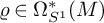 ,
$j,\,m\in {\mathbb N}$
,
$j,\,m\in {\mathbb N}$
 , and
$\varepsilon>0$
, and
$\varepsilon>0$
 small enough the equality

Since
${ \mathcal J}^{-1}(\{0\})^{\mathrm {reg}}\setminus \bigcup _{F\in {\mathcal F}^0}B_{F,\varepsilon }$
 is compact, we have a well-defined limit

which is clearly independent of the exhaustion. Let us now fix
$F\in {\mathcal F}^0$
 and focus on the corresponding summand

Since
$\{U_j\}_{j\in {\mathbb N}}$
 is an exhaustion of
${\mathscr M}_0^{\mathrm {reg}}$
is an exhaustion of
${\mathscr M}_0^{\mathrm {reg}}$
 , for all
$j\in {\mathbb N}$
, for all
$j\in {\mathbb N}$
 large enough, there exist
$R_j,r_j\in (0,\varepsilon )$
large enough, there exist
$R_j,r_j\in (0,\varepsilon )$
 with
$R_j>r_j$
with
$R_j>r_j$
 satisfying
$R_j,r_j\to 0$
satisfying
$R_j,r_j\to 0$
 as
$j\to \infty $
as
$j\to \infty $
 such that the set
$\mathscr U_{j,\varepsilon }:=\Psi _F^{-1}(\Phi _F^{-1}(\pi _0^{-1}(U_j)\cap B_{F,\varepsilon }))\subset S_F\times (0,\infty )$
such that the set
$\mathscr U_{j,\varepsilon }:=\Psi _F^{-1}(\Phi _F^{-1}(\pi _0^{-1}(U_j)\cap B_{F,\varepsilon }))\subset S_F\times (0,\infty )$
 satisfies
$S_F\times (R_j,\varepsilon )\subset \mathscr U_{j,\varepsilon }\subset S_F\times (r_j,\varepsilon )$
satisfies
$S_F\times (R_j,\varepsilon )\subset \mathscr U_{j,\varepsilon }\subset S_F\times (r_j,\varepsilon )$
 . Pulling back along
$\Psi _F$
. Pulling back along
$\Psi _F$
 and using Corollary 3.7, we get

Now, by definition (3.46) of
$\Theta _{S_F}\in \Omega ^1(Z_F,{\mathbb R})$
 one readily sees that all forms in the integrand of the right-hand side of (4.7) are bounded on the whole space
$S_F\times (0,\varepsilon )$
one readily sees that all forms in the integrand of the right-hand side of (4.7) are bounded on the whole space
$S_F\times (0,\varepsilon )$
 , except possibly the form
$\Psi _{F}^\ast \mathrm {inc}_{Z_F}^\ast \Phi _F^\ast \varrho $
, except possibly the form
$\Psi _{F}^\ast \mathrm {inc}_{Z_F}^\ast \Phi _F^\ast \varrho $
 . However, from (3.49) and (3.26) we have

so that
$\Psi _{F}$
 is simply the restriction to
$Z_F\subset \Sigma _F$
is simply the restriction to
$Z_F\subset \Sigma _F$
 of polar coordinates over
$\Sigma _F$
of polar coordinates over
$\Sigma _F$
 . Since
$\Phi _F^\ast \varrho $
. Since
$\Phi _F^\ast \varrho $
 is defined on a neighborhood of the
$0$
is defined on a neighborhood of the
$0$
 -section
$V_F\subset \Sigma _F$
-section
$V_F\subset \Sigma _F$
 rather than just on
$Z_F\cap V_F$
rather than just on
$Z_F\cap V_F$
 , one readily computes that it stays bounded in polar coordinates in the neighborhood
$V_F\subset \Sigma _F$
, one readily computes that it stays bounded in polar coordinates in the neighborhood
$V_F\subset \Sigma _F$
 of the
$0$
of the
$0$
 -section, hence its restriction
$\Psi _{F}^\ast \mathrm {inc}_{Z_F}^\ast \Phi _F^\ast \varrho $
-section, hence its restriction
$\Psi _{F}^\ast \mathrm {inc}_{Z_F}^\ast \Phi _F^\ast \varrho $
 to
$Z_F$
to
$Z_F$
 stays bounded over
$S_F\times (0,\varepsilon )$
stays bounded over
$S_F\times (0,\varepsilon )$
 as well. Therefore, the integral over the whole
$S_F\times (0,\varepsilon )$
as well. Therefore, the integral over the whole
$S_F\times (0,\varepsilon )$
 of the integrand of the right-hand side of (4.7) converges and we have a well-defined limit

which is independent of the exhaustion. This finishes the proof.
Note from Equation (4.1) that for any
$\varrho \in \Omega ^*_{S^1}(M)$
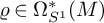 with real values, the integrand of formula (4.4) defines a signed measure on
${\mathscr M}_0^{\mathrm {reg}}$
with real values, the integrand of formula (4.4) defines a signed measure on
${\mathscr M}_0^{\mathrm {reg}}$
 up to a multiplicative constant, so that the fact that the limit (4.4) exists and is independent of the exhaustion actually shows that the integral converges in the usual sense. This is also evident from the proof of Lemma 4.4.
The following result will be used in a crucial way in Section 5.4 to establish Theorem 5.7 on the topological interpretation of the asymptotics of the Witten integral, which forms the core of the proof of Theorem 1.1.
Lemma 4.5. Let
$\sigma \in \Omega ^*_{S^1}(M)$
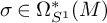 be such that for every
$F\in {\mathcal F}^0$
be such that for every
$F\in {\mathcal F}^0$
 we have
$\operatorname {{\mathrm {inc}}}_F^*\sigma \equiv 0$
we have
$\operatorname {{\mathrm {inc}}}_F^*\sigma \equiv 0$
 . Then for all
$m\in {\mathbb N}$
. Then for all
$m\in {\mathbb N}$
 , we have

where
$\kappa :\Omega _{S^1}^*(M)\to \Omega ({\mathscr M}_0^{\mathrm {reg}})$
 denotes the Kirwan map (4.3).
Proof. For any
$F\in {\mathcal F}^0$
 , recall the definition of the neighborhood (4.5) of F. Using Lemma 2.6 and the fact that the Kirwan map (4.3) is a map of complexes we can apply Stokes’ theorem to get

where the second term of the third line vanishes since the integrand is basic for the
$S^1$
 -action and therefore its top form component is zero. Next, we define for all small enough
$\varepsilon>0$
-action and therefore its top form component is zero. Next, we define for all small enough
$\varepsilon>0$
 the diffeomorphism

using the diffeomorphism
$\Psi _F$
 from (3.47), and we pull back along
$\Phi _F\circ \tilde b_{F,\varepsilon }$
from (3.47), and we pull back along
$\Phi _F\circ \tilde b_{F,\varepsilon }$
 to get

We now investigate each of the three pullbacks along
$\tilde b_{F,\varepsilon }$
 on the right-hand side. From Corollary 3.7, we get

Furthermore, we claim that for any differential form
$\alpha \in \Omega ^*(M)$
 we have

where we write
$\alpha _F:=\operatorname {{\mathrm {inc}}}_F^*\alpha \in \Omega ^*(F)$
 and we use on
$\Omega ^*(S_F)$
and we use on
$\Omega ^*(S_F)$
 the standard Fréchet topology of uniform convergence of all derivatives, recalling that
$S_F$
the standard Fréchet topology of uniform convergence of all derivatives, recalling that
$S_F$
 is compact. To prove the claim, we first note that it is enough to prove (4.13) when
$\alpha \in \Omega ^0(M)=\mathrm {C^{\infty }}(M)$
is compact. To prove the claim, we first note that it is enough to prove (4.13) when
$\alpha \in \Omega ^0(M)=\mathrm {C^{\infty }}(M)$
 is a smooth function, since (4.13) is a local formula involving pullbacks which commute with wedge products and the exterior differential d, which is a continuous operator
$\Omega ^*(S_F)\to \Omega ^*(S_F)$
is a smooth function, since (4.13) is a local formula involving pullbacks which commute with wedge products and the exterior differential d, which is a continuous operator
$\Omega ^*(S_F)\to \Omega ^*(S_F)$
 , and any differential form of positive degree can locally be written as a sum of wedge products of differentials of smooth functions. Now, by passing to a local trivialization of the fiber bundle
$\Sigma _F$
, and any differential form of positive degree can locally be written as a sum of wedge products of differentials of smooth functions. Now, by passing to a local trivialization of the fiber bundle
$\Sigma _F$
 over a local chart of F, the claim (4.13) for
$\alpha \in \mathrm {C^{\infty }}(M)$
over a local chart of F, the claim (4.13) for
$\alpha \in \mathrm {C^{\infty }}(M)$
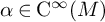 reduces to the claim that for
$n,m\in {\mathbb N}_0$
reduces to the claim that for
$n,m\in {\mathbb N}_0$
 ,
$m>0$
,
$m>0$
 , the operator

satisfies for each
$f\in \mathrm {C^{\infty }_c}({\mathbb R}^n\times {\mathbb R}^m)$
 that
that

where
$f_0(x,y):=f(x,0)$
 . One easily verifies that this holds, finishing the proof of the claim.
Combining (4.12) and (4.13) allows us to evaluate the limit in (4.11), yielding

since
$\sigma _F:=\operatorname {{\mathrm {inc}}}_F^*\sigma \equiv 0$
 by assumption. This concludes the proof.
Lemma 4.5 gives a partial cohomological interpretation for the regular Kirwan map (4.3), since it shows that the integral of the left-hand side of (4.9) does not depend on the choice of a connection with normal form near the singularities. Theorem 5.7 will actually show a posteriori that the condition
$\operatorname {{\mathrm {inc}}}_F^*\sigma \equiv 0$
 is not necessary for (4.9) to hold.
4.2 Kirwan map of a partial resolution
In order to compare our results with those in [Reference Meinrenken and Sjamaar30], let us now discuss the Kirwan map of a partial resolution. Assume that
$0\in \operatorname {\mathrm {Int}}{ \mathcal J}(M)$
 , and recall the notations of Section 3. For any connected component
$F\in {\mathcal F}^0$
, and recall the notations of Section 3. For any connected component
$F\in {\mathcal F}^0$
 of the set of fixed points
$M^{S^1}$
of the set of fixed points
$M^{S^1}$
 contained in
${ \mathcal J}^{-1}(\{0\})$
contained in
${ \mathcal J}^{-1}(\{0\})$
 we consider the complex blow-up

of
$\Sigma _F$
 along its zero section
$F\subset \Sigma _F$
along its zero section
$F\subset \Sigma _F$
 in the sense of [Reference Guillemin and Sternberg12, Section 8], which is equivariant with respect to the
$S^1$
in the sense of [Reference Guillemin and Sternberg12, Section 8], which is equivariant with respect to the
$S^1$
 -action considered in Section 3. The strict transform of the submanifold
$Z_F\subset \Sigma _F$
-action considered in Section 3. The strict transform of the submanifold
$Z_F\subset \Sigma _F$
 introduced in (3.6) is defined as the closure
${\widetilde {Z}_F:= \overline {\beta _{\widetilde {\Sigma }_F}^{-1}(Z_F)}\subset \widetilde {\Sigma }_F}$
introduced in (3.6) is defined as the closure
${\widetilde {Z}_F:= \overline {\beta _{\widetilde {\Sigma }_F}^{-1}(Z_F)}\subset \widetilde {\Sigma }_F}$
 and inherits a natural structure of a smooth
$S^1$
and inherits a natural structure of a smooth
$S^1$
 -submanifold of
$\widetilde {\Sigma }_F$
-submanifold of
$\widetilde {\Sigma }_F$
 . Setting
$\mathbb {F}^0:=\sqcup _{F\in {\mathcal F}^0} F\subset M^{S^1}$
. Setting
$\mathbb {F}^0:=\sqcup _{F\in {\mathcal F}^0} F\subset M^{S^1}$
 we then define the complex blow-up of M along
$\mathbb {F}^0\subset M$
we then define the complex blow-up of M along
$\mathbb {F}^0\subset M$
 as the unique
$S^1$
as the unique
$S^1$
 -equivariant map

which restricts to an
$S^1$
 -equivariant diffeomorphism over
$M\setminus \mathbb {F}^0$
-equivariant diffeomorphism over
$M\setminus \mathbb {F}^0$
 and which, over each open set
$U_F\subset M$
and which, over each open set
$U_F\subset M$
 as in Proposition 3.2 is given by the map
$\beta _{\widetilde {\Sigma }_F}$
as in Proposition 3.2 is given by the map
$\beta _{\widetilde {\Sigma }_F}$
 over
$V_F$
over
$V_F$
 . Like
$\widetilde Z_F$
. Like
$\widetilde Z_F$
 , the strict transform
$\widetilde Z$
, the strict transform
$\widetilde Z$
 of the subset
${ \mathcal J}^{-1}(\{0\})^{\mathrm {reg}}\subset M$
of the subset
${ \mathcal J}^{-1}(\{0\})^{\mathrm {reg}}\subset M$
 is defined as the closure
${\widetilde Z:=\overline {\beta ^{-1} ({ \mathcal J}^{-1}(\{0\})^{{\mathrm {reg}}})}\subset \widetilde M}$
is defined as the closure
${\widetilde Z:=\overline {\beta ^{-1} ({ \mathcal J}^{-1}(\{0\})^{{\mathrm {reg}}})}\subset \widetilde M}$
 and inherits a natural structure of a smooth
$S^1$
and inherits a natural structure of a smooth
$S^1$
 -submanifold of
$\widetilde M$
-submanifold of
$\widetilde M$
 . Since the
$S^1$
. Since the
$S^1$
 -action on
$\widetilde Z$
-action on
$\widetilde Z$
 is locally free, one is led to the following definition.
Definition 4.6. The partial resolution of the symplectic quotient
${\mathscr M}_0$
 is defined as the orbifold

together with the map
$\beta _0:\widetilde {\mathscr M}_0\longrightarrow {\mathscr M}_0$
 induced by the map (4.15) after taking quotients by the
$S^1$
induced by the map (4.15) after taking quotients by the
$S^1$
 -action. The unique form
$\widetilde \omega _0\in \Omega ^2(\widetilde {\mathscr M}_0,{\mathbb R})$
-action. The unique form
$\widetilde \omega _0\in \Omega ^2(\widetilde {\mathscr M}_0,{\mathbb R})$
 satisfying

where
$\widetilde \pi _0:\widetilde Z\longrightarrow \widetilde {\mathscr M}_0$
 denotes the quotient map, is called the degenerate symplectic form of
$\widetilde {\mathscr M}_0$
denotes the quotient map, is called the degenerate symplectic form of
$\widetilde {\mathscr M}_0$
 .
.
Partial resolutions were introduced for arbitrary compact Lie group actions by Kirwan in [Reference Kirwan22] in the algebraic case and by Meinrenken and Sjamaar in [Reference Meinrenken and Sjamaar30, Section 4.1.2] in the symplectic case. As it is explained in [Reference Delarue, Ramacher and Schmitt7, Corollary 3.14], our definition agrees with this definition in the case
$G=S^1$
 .
.
We now define the following alternative notion of a Kirwan map for singular symplectic quotients by an
$S^1$
 -action, even though
$\widetilde M$
-action, even though
$\widetilde M$
 does not admit a canonical structure of a Hamiltonian
$S^1$
does not admit a canonical structure of a Hamiltonian
$S^1$
 -manifold.
Definition 4.7. The resolution Kirwan map is the map

where
$\beta ^*:H^*_{S^1}(M)\to H^*_{S^1}(\widetilde M)$
 is induced by the map (4.15) and
$\kappa :H^*_{S^1}(\widetilde {M})\longrightarrow H^*(\widetilde {\mathscr M}_0)$
is induced by the map (4.15) and
$\kappa :H^*_{S^1}(\widetilde {M})\longrightarrow H^*(\widetilde {\mathscr M}_0)$
 is defined at the level of complexes by the formula (4.1) with
$\operatorname {{\mathrm {inc}}}_0:{ \mathcal J}^{-1}(\{0\})\to M$
is defined at the level of complexes by the formula (4.1) with
$\operatorname {{\mathrm {inc}}}_0:{ \mathcal J}^{-1}(\{0\})\to M$
 replaced by the inclusion map
$\operatorname {{\mathrm {inc}}}_{\widetilde Z}:\widetilde Z\to \widetilde M$
replaced by the inclusion map
$\operatorname {{\mathrm {inc}}}_{\widetilde Z}:\widetilde Z\to \widetilde M$
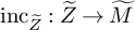 .
.
The following result gives another topological interpretation of the regular Kirwan map (4.3), strengthening Lemma 4.5 under an appropriate combinatorial condition on the
$S^1$
 -action around the fixed points.
Lemma 4.8. With the notation of Section 3.1, assume that the weights of the
$S^1$
 -action satisfy the condition

for each
$F\in {\mathcal F}^0$
 . Then, for any connection
$\Theta \in \Omega ^1({ \mathcal J}^{-1}(\{0\})^{\mathrm {reg}},{\mathbb R})$
. Then, for any connection
$\Theta \in \Omega ^1({ \mathcal J}^{-1}(\{0\})^{\mathrm {reg}},{\mathbb R})$
 with normal form near the singularities in the sense of Definition 4.2 there exists a connection
$\widetilde \Theta \in \Omega ^1(\widetilde Z,{\mathbb R})$
with normal form near the singularities in the sense of Definition 4.2 there exists a connection
$\widetilde \Theta \in \Omega ^1(\widetilde Z,{\mathbb R})$
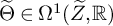 for the
$S^1$
for the
$S^1$
 -action on the strict transform
$\widetilde Z$
-action on the strict transform
$\widetilde Z$
 satisfying

In particular, for any
$\varrho \in \Omega _{S^1}^*(M)$
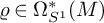 we have

Proof. Let
$F\in {\mathcal F}^0$
 and equip the complex vector bundle
$\nu _F:\Sigma _F\to F$
and equip the complex vector bundle
$\nu _F:\Sigma _F\to F$
 with the Hermitian norm
$\frac {1}{\sqrt {2}}\|\cdot \|_F$
with the Hermitian norm
$\frac {1}{\sqrt {2}}\|\cdot \|_F$
 defined by Equation (3.11). Write
$\nu _{\mathscr {S}_F}:\mathscr {S}_F\to F$
defined by Equation (3.11). Write
$\nu _{\mathscr {S}_F}:\mathscr {S}_F\to F$
 for the associated unit sphere bundle and consider the natural diffeomorphism

Then, the bi-ellipsoid bundle
$S_F\to F$
 defined in (3.44) satisfies
$S_F\subset \mathscr {S}_F$
defined in (3.44) satisfies
$S_F\subset \mathscr {S}_F$
 . Next, using the notation (3.35), let us set

Comparing with Equations (3.37) and (3.41) one gets the identity
$\Theta _{S_F}=\operatorname {{\mathrm {inc}}}_{S_F}^*\Theta _{\mathscr {S}_F}$
 , while via the restricted diffeomorphism (3.49) one has
$\Psi _F^*\Theta _{Z_F}=\mathrm {pr}_{S_F}^*\Theta _{S_F}$
, while via the restricted diffeomorphism (3.49) one has
$\Psi _F^*\Theta _{Z_F}=\mathrm {pr}_{S_F}^*\Theta _{S_F}$
 . On the other hand, by Definitions (3.13) and (3.14) one readily checks that (4.21) is basic for the
$S^1$
. On the other hand, by Definitions (3.13) and (3.14) one readily checks that (4.21) is basic for the
$S^1$
 -action over
$\mathscr {S}_F$
-action over
$\mathscr {S}_F$
 induced by multiplication with
$e^{2\pi i\theta }\in {\mathbb C}^*$
induced by multiplication with
$e^{2\pi i\theta }\in {\mathbb C}^*$
 for all
$\theta \in {\mathbb R}/{\mathbb Z}$
for all
$\theta \in {\mathbb R}/{\mathbb Z}$
 if and only if the condition (4.17) is satisfied. Write
$\vartheta _F\in \Omega ^1(\Sigma _F\backslash F,{\mathbb R})$
if and only if the condition (4.17) is satisfied. Write
$\vartheta _F\in \Omega ^1(\Sigma _F\backslash F,{\mathbb R})$
 for the unique form over the complement of the zero section inside
$\Sigma _F$
for the unique form over the complement of the zero section inside
$\Sigma _F$
 satisfying
$\Psi _{\mathscr {S}_F}^*\vartheta _F =\mathrm {pr}_{\mathscr {S}_F}^*\Theta _{\mathscr {S}_F}$
satisfying
$\Psi _{\mathscr {S}_F}^*\vartheta _F =\mathrm {pr}_{\mathscr {S}_F}^*\Theta _{\mathscr {S}_F}$
 . Then, according to [Reference Guillemin and Sternberg12, Section 11] there exists a unique form
$\widetilde \vartheta _F\in \Omega ^1(\widetilde {\Sigma }_F,{\mathbb R})$
. Then, according to [Reference Guillemin and Sternberg12, Section 11] there exists a unique form
$\widetilde \vartheta _F\in \Omega ^1(\widetilde {\Sigma }_F,{\mathbb R})$
 satisfying

By restricting
$\widetilde \vartheta _F$
 to
$\widetilde {Z}_F\subset \widetilde {\Sigma }_F$
to
$\widetilde {Z}_F\subset \widetilde {\Sigma }_F$
 one gets a form
${\Theta }_{\widetilde Z_F}\in \Omega ^1(\widetilde {Z}_F,{\mathbb R})$
one gets a form
${\Theta }_{\widetilde Z_F}\in \Omega ^1(\widetilde {Z}_F,{\mathbb R})$
 satisfying

In view of Definition 4.2 of a connection
$\Theta \in \Omega ^1({ \mathcal J}^{-1}(\{0\})^{\mathrm {reg}},{\mathbb R})$
 with normal form near the singularities this concludes the proof of (4.18). Formula (4.19) is then a straightforward consequence of the Definitions 4.3 and 4.7 of the regular and resolution Kirwan maps, using the fact that
$ \beta ^{-1}_0({\mathscr M}_0^{\text {reg}})$
with normal form near the singularities this concludes the proof of (4.18). Formula (4.19) is then a straightforward consequence of the Definitions 4.3 and 4.7 of the regular and resolution Kirwan maps, using the fact that
$ \beta ^{-1}_0({\mathscr M}_0^{\text {reg}})$
 is of full measure inside
$\widetilde {\mathscr M}_0$
is of full measure inside
$\widetilde {\mathscr M}_0$
 .
.
Lemma 4.8 shows that, under the combinatorial condition (4.17), the first term in (1.10) can be interpreted topologically in terms of the partial resolution
$\widetilde {\mathscr M}_0$
 of
${\mathscr M}$
of
${\mathscr M}$
 introduced in Definition 4.6. We will show in Section 6.3 that this condition is actually realized on a large class of examples.
Remark 4.9. It is instructive to compare the resolution Kirwan map of Definition 4.7 with the Kirwan map considered by Jeffrey, Kiem, Kirwan, and Woolf in [Reference Jeffrey, Kiem, Kirwan and Woolf16] in the case
$G=S^1$
 . They work in the complex case, so that
${\mathscr M}_0$
. They work in the complex case, so that
${\mathscr M}_0$
 is obtained as a GIT quotient by a
${\mathbb C}^*$
is obtained as a GIT quotient by a
${\mathbb C}^*$
 -action of a smooth projective variety M, and work instead with the so-called intersection cohomology
$IH^{*}({\mathscr M}_{0})$
-action of a smooth projective variety M, and work instead with the so-called intersection cohomology
$IH^{*}({\mathscr M}_{0})$
 of the singular quotient. Relying on the fact that the intersection cohomology naturally occurs as a summand inside the usual cohomology
$H^{*}(\widetilde {\mathscr M}_{0})$
of the singular quotient. Relying on the fact that the intersection cohomology naturally occurs as a summand inside the usual cohomology
$H^{*}(\widetilde {\mathscr M}_{0})$
 of the partial resolution
$\widetilde {\mathscr M}_0$
of the partial resolution
$\widetilde {\mathscr M}_0$
 of Definition 4.6, they consider the canonical map

obtained by composition of the resolution Kirwan map
$\widetilde \kappa :H^*_{S^1}(M)\longrightarrow H^*(\widetilde {\mathscr M}_0)$
 of Definition 4.7 with the canonical projection from
$H^{*}(\widetilde {\mathscr M}_{0})$
of Definition 4.7 with the canonical projection from
$H^{*}(\widetilde {\mathscr M}_{0})$
 onto the summand
$IH^{*}({\mathscr M}_{0})$
onto the summand
$IH^{*}({\mathscr M}_{0})$
 . Nevertheless, in the general symplectic setting, the relation between
$IH^{*}({\mathscr M}_{0})$
. Nevertheless, in the general symplectic setting, the relation between
$IH^{*}({\mathscr M}_{0})$
 and
$H^{*}(\widetilde {\mathscr M}_{0})$
and
$H^{*}(\widetilde {\mathscr M}_{0})$
 is not as clear as in the complex setting considered in [Reference Jeffrey, Kiem, Kirwan and Woolf16], and there might not be a canonical choice of an intersection Kirwan map in general.
5 Asymptotic expansion of the Witten integral
We shall now introduce the Witten integral, which is our main tool in our approach to geometric quantization of singular symplectic quotients. We work in the setting of Section 3.1, so that
$G=S^1$
 and the identification
$\mathbf {\mathfrak g}\simeq {\mathbb R}$
and the identification
$\mathbf {\mathfrak g}\simeq {\mathbb R}$
 of (2.6) is understood. Recall in particular the identification (2.7) of
$\Omega _{S^1}^\ast (M)$
of (2.6) is understood. Recall in particular the identification (2.7) of
$\Omega _{S^1}^\ast (M)$
 with the space of
$S^1$
with the space of
$S^1$
 -invariant differential forms with values in entire analytic series of the variable
$x\in {\mathbb R}$
-invariant differential forms with values in entire analytic series of the variable
$x\in {\mathbb R}$
 , and the identification (2.11) of the moment map with a real-valued function
${ \mathcal J}:M\to {\mathbb R}$
, and the identification (2.11) of the moment map with a real-valued function
${ \mathcal J}:M\to {\mathbb R}$
 .
.
Definition 5.1. For any equivariantly closed
$\varrho \in \Omega _{S^1}^\ast (M)$
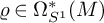 and any test function
${\phi \in \mathrm {C^{\infty }_c}({\mathbb R})}$
and any test function
${\phi \in \mathrm {C^{\infty }_c}({\mathbb R})}$
 , the associated Witten integral depending on a parameter
$m\in {\mathbb N}$
, the associated Witten integral depending on a parameter
$m\in {\mathbb N}$
 is given by the formula

The precise form of the exponents in (5.1) is determined by our conventions in (2.10) and (2.1), as it is crucial that
$\bar \omega (X):=\omega +2\pi i{ \mathcal J}(X)\in \Omega ^*_{S^1}(M)$
 is equivariantly closed. In (5.1),
$\phi \in \mathrm {C^{\infty }_c}({\mathbb R})$
is equivariantly closed. In (5.1),
$\phi \in \mathrm {C^{\infty }_c}({\mathbb R})$
 plays the role of a test function at which the distribution
${\mathcal W}_m(\varrho )\in \mathcal {\mathcal D}'({\mathbb R}) $
plays the role of a test function at which the distribution
${\mathcal W}_m(\varrho )\in \mathcal {\mathcal D}'({\mathbb R}) $
 is evaluated, and this distribution is the object that we are primarily interested in, the main goal being a description of the asymptotic behaviour of
${\mathcal W}_m(\varrho ) $
is evaluated, and this distribution is the object that we are primarily interested in, the main goal being a description of the asymptotic behaviour of
${\mathcal W}_m(\varrho ) $
 as
$m \to \infty $
as
$m \to \infty $
 .
.
The analytic difficulties underlying the study of the asymptotic behaviour of the Witten integral have already been overcome in the previous work [Reference Delarue and Ramacher6]. In that work the problem of deriving asymptotics of (5.1) as
$m\to \infty $
 is considered in the more general setting of studying the asymptotic behaviour of so-called generalized Witten integrals

as
$\varepsilon \to 0^+$
 , with amplitudes
$a\in \mathrm {C^{\infty }_c}(M)$
, with amplitudes
$a\in \mathrm {C^{\infty }_c}(M)$
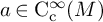 ,
$\phi \in \mathrm {C^{\infty }_c}({\mathbb R})$
,
$\phi \in \mathrm {C^{\infty }_c}({\mathbb R})$
 , and phase function
$\psi \in \mathrm {C^{\infty }}(M\times {\mathbb R})$
, and phase function
$\psi \in \mathrm {C^{\infty }}(M\times {\mathbb R})$
 given by
$\psi (p,x):=2\pi { \mathcal J}(p)(x)$
given by
$\psi (p,x):=2\pi { \mathcal J}(p)(x)$
 ,
$dM:={\omega ^n}/{n!}$
,
$dM:={\omega ^n}/{n!}$
 being the symplectic volume form on M. Since the critical set

is not clean unless
$0$
 is a regular value of
${ \mathcal J}$
is a regular value of
${ \mathcal J}$
 , the stationary phase principle cannot be applied. Instead, a complete asymptotic expansion for integrals of the form (5.2) was derived in [Reference Delarue and Ramacher6, Theorem 1.1] via a process called destratification, the coefficients in the asymptotics being given by integrals over the strata of the singular symplectic quotient
${\mathscr M}_0$
, the stationary phase principle cannot be applied. Instead, a complete asymptotic expansion for integrals of the form (5.2) was derived in [Reference Delarue and Ramacher6, Theorem 1.1] via a process called destratification, the coefficients in the asymptotics being given by integrals over the strata of the singular symplectic quotient
${\mathscr M}_0$
 . From this, the existence of an expansion of (5.1), and also some rough properties of its coefficients, can be inferred. However, within that more general framework the equivariant-cohomological interpretation of the coefficients in the obtained expansion remains elusive. Therefore, we shall not use the results derived there but proceed from scratch, based on the fact that the amplitude in the Witten integral is an equivariantly closed form, which allows a simpler and concise treatment.
5.1 Preliminaries
We begin now with the study of the asymptotics of the Witten integral 5.1. Conceptually, we will follow the method of Meinrenken in [Reference Meinrenken28, Proof of Theorem 3.3], the crucial idea being a retraction onto the zero level set of the moment map and the use of the equivariant homotopy Lemma 2.3 and equivariant Stokes’ Lemma 2.2, combined with the classical stationary phase principle. But since we do not assume zero to be a regular value of the moment map, the situation is much more involved. In fact, we will combine a retraction onto the regular stratum of
${ \mathcal J}^{-1}(\left \{ 0 \right \})$
 with retractions onto the several components of the singular stratum of
${ \mathcal J}^{-1}(\left \{ 0 \right \})$
with retractions onto the several components of the singular stratum of
${ \mathcal J}^{-1}(\left \{ 0 \right \})$
 .
.
As a first step, we choose – once and for all – for each
$F\in {\mathcal F}$
 open sets
$U_F\subset M$
open sets
$U_F\subset M$
 and
$V_F\subset \Sigma _F$
and
$V_F\subset \Sigma _F$
 as in Proposition 3.2. For technical purposes, we choose them small enough such that the symplectic form (3.40) is actually non-degenerate on a slightly larger tubular neighborhood
$\widetilde V_F\subset \Sigma _F$
as in Proposition 3.2. For technical purposes, we choose them small enough such that the symplectic form (3.40) is actually non-degenerate on a slightly larger tubular neighborhood
$\widetilde V_F\subset \Sigma _F$
 of the zero section of
$\Sigma _F$
of the zero section of
$\Sigma _F$
 containing
$\overline V_F$
containing
$\overline V_F$
 , so that Proposition 3.2 applies to a corresponding neighborhood
$\widetilde U_F\subset M$
, so that Proposition 3.2 applies to a corresponding neighborhood
$\widetilde U_F\subset M$
 containing
$\overline U_F$
containing
$\overline U_F$
 with a symplectomorphism
$\widetilde \Phi _F:\widetilde V_F\to \widetilde U_F$
with a symplectomorphism
$\widetilde \Phi _F:\widetilde V_F\to \widetilde U_F$
 extending
$\Phi _F$
extending
$\Phi _F$
 , while keeping the sets
$\widetilde U_F$
, while keeping the sets
$\widetilde U_F$
 obtained for the different F disjoint. This setup will be kept fixed in all of the following.
Lemma 5.2. There exists
$\delta>0$
 and an
$S^1$
and an
$S^1$
 -invariant open neighborhood
$W\subset M\setminus M^{S^1}$
-invariant open neighborhood
$W\subset M\setminus M^{S^1}$
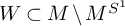 of
${ \mathcal J}^{-1}(\{0\})^{\mathrm {reg}}$
of
${ \mathcal J}^{-1}(\{0\})^{\mathrm {reg}}$
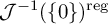 together with a retraction
$\mathrm {ret}_0:W\to { \mathcal J}^{-1}(\{0\})^{\mathrm {reg}}$
together with a retraction
$\mathrm {ret}_0:W\to { \mathcal J}^{-1}(\{0\})^{\mathrm {reg}}$
 and an
$S^1$
and an
$S^1$
 -equivariant diffeomorphism

such that, in case
$0\in \operatorname {\mathrm {Int}}\,J(M)$
 , we have
$\Phi _F^{-1}(U_F\cap W)\subset \Sigma _{F\bullet \bullet }$
, we have
$\Phi _F^{-1}(U_F\cap W)\subset \Sigma _{F\bullet \bullet }$
 for all
$F\in {\mathcal F}^0$
for all
$F\in {\mathcal F}^0$
 and
and

while
$W\cap \widetilde {U}_F=\emptyset $
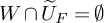 in case
$0\in \partial \,{ \mathcal J}(M)$
in case
$0\in \partial \,{ \mathcal J}(M)$
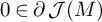 .
.
Proof. Let
$g^{TM}$
 be an
$S^1$
be an
$S^1$
 -invariant Riemannian metric on M satisfying
$\Phi _F^*(g^{TM}|_{\widetilde {U}_F})=g^{T\Sigma _F}$
-invariant Riemannian metric on M satisfying
$\Phi _F^*(g^{TM}|_{\widetilde {U}_F})=g^{T\Sigma _F}$
 in the local normal form coordinates of Proposition 3.2 for all
$F\in {\mathcal F}$
in the local normal form coordinates of Proposition 3.2 for all
$F\in {\mathcal F}$
 . Write
$\mathrm {grad}\,{ \mathcal J}\in \mathrm {C^{\infty }}(M,TM)$
. Write
$\mathrm {grad}\,{ \mathcal J}\in \mathrm {C^{\infty }}(M,TM)$
 for the associated Riemannian gradient of
${ \mathcal J}:M\to {\mathbb R}$
for the associated Riemannian gradient of
${ \mathcal J}:M\to {\mathbb R}$
 , and let
$\xi \in \mathrm {C^{\infty }}(M\backslash M^{S^1},TM)$
, and let
$\xi \in \mathrm {C^{\infty }}(M\backslash M^{S^1},TM)$
 be the vector field

where we use that the Hamiltonian
$S^1$
 -action is locally free on
$M\backslash M^{S^1}$
-action is locally free on
$M\backslash M^{S^1}$
 , so that
$\mathrm {grad}\,{ \mathcal J}$
, so that
$\mathrm {grad}\,{ \mathcal J}$
 is nowhere vanishing on
$M\backslash M^{S^1}$
is nowhere vanishing on
$M\backslash M^{S^1}$
 . In case
$0\in \operatorname {\mathrm {Int}}{ \mathcal J}(M)$
. In case
$0\in \operatorname {\mathrm {Int}}{ \mathcal J}(M)$
 , the vector field (5.5) is transverse to
${ \mathcal J}^{-1}(\{0\})^{\mathrm {reg}}$
, the vector field (5.5) is transverse to
${ \mathcal J}^{-1}(\{0\})^{\mathrm {reg}}$
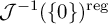 , satisfies
$d{ \mathcal J}\mathbin {\lrcorner } \xi =1$
, satisfies
$d{ \mathcal J}\mathbin {\lrcorner } \xi =1$
 over
$M\backslash M^{S^1}$
over
$M\backslash M^{S^1}$
 , and in view of (3.27) is mapped to the vector field
$\frac {\partial }{\partial q}$
, and in view of (3.27) is mapped to the vector field
$\frac {\partial }{\partial q}$
 by the diffeomorphism of Proposition 3.2 over
$\widetilde U_F\subset M$
by the diffeomorphism of Proposition 3.2 over
$\widetilde U_F\subset M$
 for each
${F\in {\mathcal F}^0}$
for each
${F\in {\mathcal F}^0}$
 . From this explicit description near each
$F\in {\mathcal F}^0$
. From this explicit description near each
$F\in {\mathcal F}^0$
 and the fact that the set
${K:={ \mathcal J}^{-1}(\{0\})^{\mathrm {reg}}\cap (M\setminus \bigcup _{F\in {\mathcal F}^0} U_F)}$
and the fact that the set
${K:={ \mathcal J}^{-1}(\{0\})^{\mathrm {reg}}\cap (M\setminus \bigcup _{F\in {\mathcal F}^0} U_F)}$
 is compact, it follows that there is a
$\delta>0$
is compact, it follows that there is a
$\delta>0$
 such that the flow
$\Phi _t^{\xi }$
such that the flow
$\Phi _t^{\xi }$
 of
$\xi $
of
$\xi $
 is defined on
${ \mathcal J}^{-1}(\{0\})^{\mathrm {reg}}$
is defined on
${ \mathcal J}^{-1}(\{0\})^{\mathrm {reg}}$
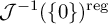 for all
$t\in (-\delta ,\delta )$
for all
$t\in (-\delta ,\delta )$
 . Consequently, the smooth map

is a diffeomorphism onto its image satisfying
${ \mathcal J}(\Phi ^{\xi }(p,t))=t$
 for all
$p\in { \mathcal J}^{-1}(\{0\})^{\mathrm {reg}}$
for all
$p\in { \mathcal J}^{-1}(\{0\})^{\mathrm {reg}}$
 and
$t\in (-\delta ,\delta )$
and
$t\in (-\delta ,\delta )$
 . Setting
$W:=\mathrm {im}(\Phi ^{\xi })\subset M$
. Setting
$W:=\mathrm {im}(\Phi ^{\xi })\subset M$
 , we define the diffeomorphism (5.3) to be the inverse of (5.6). Recalling the definition of
$\mathrm {ret}_{Z_F}$
, we define the diffeomorphism (5.3) to be the inverse of (5.6). Recalling the definition of
$\mathrm {ret}_{Z_F}$
 in (3.48), all claimed properties except the last one are satisfied by construction. Finally, in the case
$0\in \partial \,{ \mathcal J}(M)$
in (3.48), all claimed properties except the last one are satisfied by construction. Finally, in the case
$0\in \partial \,{ \mathcal J}(M)$
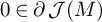 , then K is disjoint from
$\bigcup _{F\in {\mathcal F}^0} \widetilde U_F$
, then K is disjoint from
$\bigcup _{F\in {\mathcal F}^0} \widetilde U_F$
 simply because
${ \mathcal J}^{-1}(\{0\})^{\mathrm {reg}}$
simply because
${ \mathcal J}^{-1}(\{0\})^{\mathrm {reg}}$
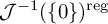 is disjoint from
$\widetilde U_F$
is disjoint from
$\widetilde U_F$
 . Hence in that case, it suffices to take
$\delta $
. Hence in that case, it suffices to take
$\delta $
 small enough to get that
$W\cap \widetilde {U}_F=\emptyset $
small enough to get that
$W\cap \widetilde {U}_F=\emptyset $
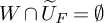 for all
$F\in {\mathcal F}^0$
for all
$F\in {\mathcal F}^0$
 .
.
The following simple consequence of the equivariant Stokes’ Lemma 2.2 and the equivariant homotopy Lemma 2.3 will allow us to greatly simplify the computations of the next section.
Lemma 5.3. The Witten integral of Definition 5.1 only depends on the equivariant cohomology class of
$\varrho \in \Omega _{S^1}^\ast (M)$
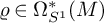 inside
$H_{S^1}^*(M)$
inside
$H_{S^1}^*(M)$
 . Moreover, each equivariant cohomology class in
$H_{S^1}^*(M)$
. Moreover, each equivariant cohomology class in
$H_{S^1}^*(M)$
 has a representative
$\varrho \in \Omega _{S^1}^\ast (M)$
has a representative
$\varrho \in \Omega _{S^1}^\ast (M)$
 satisfying

and

where
$\operatorname {{\mathrm {ret}}}_{0}:W\to { \mathcal J}^{-1}(\{0\})^{\mathrm {reg}}$
 is as in Lemma 5.2 with a suitable
$\delta>0$
is as in Lemma 5.2 with a suitable
$\delta>0$
 and
$\text {inc}_0:{ \mathcal J}^{-1}(\{0\})^{\mathrm {reg}}\to M$
and
$\text {inc}_0:{ \mathcal J}^{-1}(\{0\})^{\mathrm {reg}}\to M$
 denotes the inclusion map.
Proof. The first claim is standard. Indeed, let
$\varrho \in \Omega _{S^1}^\ast (M)$
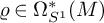 be equivariantly closed. In view of the fact that
$ e^{2\pi im{ \mathcal J}(x)} e^{m \omega }\in \Omega _{S^1}^\ast (M)$
be equivariantly closed. In view of the fact that
$ e^{2\pi im{ \mathcal J}(x)} e^{m \omega }\in \Omega _{S^1}^\ast (M)$
 is equivariantly closed, Lemma 2.2 implies for any equivariant form
$\gamma \in \Omega _{S^1}^\ast (M)$
is equivariantly closed, Lemma 2.2 implies for any equivariant form
$\gamma \in \Omega _{S^1}^\ast (M)$
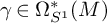 that
that

proving the first claim of the lemma.
Let us consider now an arbitrary equivariantly closed
$\widetilde \varrho \in \Omega _{S^1}^\ast (M)$
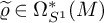 . To prove the remaining assertions of the lemma, we need to construct an equivariantly closed
${\varrho \in \Omega _{S^1}^\ast (M)}$
. To prove the remaining assertions of the lemma, we need to construct an equivariantly closed
${\varrho \in \Omega _{S^1}^\ast (M)}$
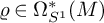 in the cohomology class
$[\widetilde \varrho ]\in H_{S^1}^*(M)$
in the cohomology class
$[\widetilde \varrho ]\in H_{S^1}^*(M)$
 satisfying (5.7) and (5.8). Using Lemma 2.3 with
$N=F$
satisfying (5.7) and (5.8). Using Lemma 2.3 with
$N=F$
 and
$U_N=\widetilde U_F$
and
$U_N=\widetilde U_F$
 we get for each
$F\in {\mathcal F}^0$
we get for each
$F\in {\mathcal F}^0$
 an equivariant form
$\gamma _F\in \Omega _{S^1}^\ast (\widetilde V_F)$
an equivariant form
$\gamma _F\in \Omega _{S^1}^\ast (\widetilde V_F)$
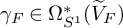 such that

Let
$\chi _F\in \mathrm {C^{\infty }}(M)$
 have compact support in
$\widetilde U_F$
have compact support in
$\widetilde U_F$
 and be identically equal to
$1$
and be identically equal to
$1$
 on
$U_F$
on
$U_F$
 . Setting

the equivariantly closed form
$\widehat \varrho :=\widetilde \varrho -d_{\mathbf {\mathfrak g}}\gamma \in \Omega _{S^1}^\ast (M)$
 satisfies
$\widetilde \Phi _{F}^\ast ( \widehat \varrho |_{U_F}) = (\nu _{\Sigma _F}^\ast \operatorname {{\mathrm {inc}}}_F^\ast \widetilde \varrho )|_{V_F}$
satisfies
$\widetilde \Phi _{F}^\ast ( \widehat \varrho |_{U_F}) = (\nu _{\Sigma _F}^\ast \operatorname {{\mathrm {inc}}}_F^\ast \widetilde \varrho )|_{V_F}$
 . But
$\nu _{\Sigma _F}\circ \widetilde \Phi _F^{-1}\circ \mathrm {inc}_F=\mathrm {inc}_F$
. But
$\nu _{\Sigma _F}\circ \widetilde \Phi _F^{-1}\circ \mathrm {inc}_F=\mathrm {inc}_F$
 , so that (5.9) implies for each
$F\in {\mathcal F}^0$
, so that (5.9) implies for each
$F\in {\mathcal F}^0$


yielding
$\mathrm {inc}_F^*\widehat \varrho =\mathrm {inc}_F^*\widetilde \varrho $
 and consequently

Next, choose
$\delta>0$
 in Lemma 5.2 such that it applies also with a slightly larger
$\widehat \delta>\delta $
in Lemma 5.2 such that it applies also with a slightly larger
$\widehat \delta>\delta $
 and gives us two corresponding retractions
$\widehat {\operatorname {{\mathrm {ret}}}}_{0}:\widehat W\to { \mathcal J}^{-1}(\{0\})^{\mathrm {reg}}$
and gives us two corresponding retractions
$\widehat {\operatorname {{\mathrm {ret}}}}_{0}:\widehat W\to { \mathcal J}^{-1}(\{0\})^{\mathrm {reg}}$
 and
$\operatorname {{\mathrm {ret}}}_{0}:W\to { \mathcal J}^{-1}(\{0\})^{\mathrm {reg}}$
and
$\operatorname {{\mathrm {ret}}}_{0}:W\to { \mathcal J}^{-1}(\{0\})^{\mathrm {reg}}$
 from open subsets
$\widehat W,W\subset M$
from open subsets
$\widehat W,W\subset M$
 onto
$J^{-1}(\{0\})^{\mathrm {reg}}$
onto
$J^{-1}(\{0\})^{\mathrm {reg}}$
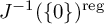 such that
$\widehat {\operatorname {{\mathrm {ret}}}}_{0}|_{W}=\operatorname {{\mathrm {ret}}}_{0}$
such that
$\widehat {\operatorname {{\mathrm {ret}}}}_{0}|_{W}=\operatorname {{\mathrm {ret}}}_{0}$
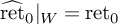 . Let
$\overline {W}$
. Let
$\overline {W}$
 be the closure of W in M. Then the compact set
$\overline {W}\setminus \bigcup _{F\in {\mathcal F}^0}U_F$
be the closure of W in M. Then the compact set
$\overline {W}\setminus \bigcup _{F\in {\mathcal F}^0}U_F$
 lies in
$M\setminus M^{S^1}$
lies in
$M\setminus M^{S^1}$
 and its intersection with
$J^{-1}(\{0\})^{\mathrm {reg}}$
and its intersection with
$J^{-1}(\{0\})^{\mathrm {reg}}$
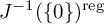 is compact. By making
$\delta $
is compact. By making
$\delta $
 , and hence W, smaller while keeping
$\widehat \delta $
, and hence W, smaller while keeping
$\widehat \delta $
 fixed, we can therefore achieve that
$\widehat W$
fixed, we can therefore achieve that
$\widehat W$
 contains
$\overline {W}\setminus \bigcup _{F\in {\mathcal F}^0}U_F$
contains
$\overline {W}\setminus \bigcup _{F\in {\mathcal F}^0}U_F$
 . Using Lemma 2.3 again, now with
$N={ \mathcal J}^{-1}(\{0\})^{\mathrm {reg}}$
. Using Lemma 2.3 again, now with
$N={ \mathcal J}^{-1}(\{0\})^{\mathrm {reg}}$
 and
$U_N=\widehat W$
and
$U_N=\widehat W$
 , there is a form
$\sigma \in \Omega _{S^1}^\ast (\widehat W)$
, there is a form
$\sigma \in \Omega _{S^1}^\ast (\widehat W)$
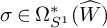 such that

On the other hand, in case
$0\in \operatorname {\mathrm {Int}}{ \mathcal J}(M)$
 , for any
$F\in {\mathcal F}^0$
, for any
$F\in {\mathcal F}^0$
 one has
$\nu _{\Sigma _F}\circ \operatorname {{\mathrm {inc}}}_{Z_F}\circ \operatorname {{\mathrm {ret}}}_{Z_F}=\nu _{\Sigma _F|\Sigma _{F\bullet \bullet }}$
one has
$\nu _{\Sigma _F}\circ \operatorname {{\mathrm {inc}}}_{Z_F}\circ \operatorname {{\mathrm {ret}}}_{Z_F}=\nu _{\Sigma _F|\Sigma _{F\bullet \bullet }}$
 so that from (5.10) we deduce that
$\widetilde \Phi _{F}^\ast (\widehat \varrho |_{\widehat W \cap U_F}) =\operatorname {{\mathrm {ret}}}_{Z_F}^*\operatorname {{\mathrm {inc}}}_{Z_F}^*\widetilde \Phi _{F}^\ast (\widehat \varrho |_{\widehat W \cap U_F})$
so that from (5.10) we deduce that
$\widetilde \Phi _{F}^\ast (\widehat \varrho |_{\widehat W \cap U_F}) =\operatorname {{\mathrm {ret}}}_{Z_F}^*\operatorname {{\mathrm {inc}}}_{Z_F}^*\widetilde \Phi _{F}^\ast (\widehat \varrho |_{\widehat W \cap U_F})$
 for such an F. Thanks to Lemma 5.2 we therefore already know that

Invoking the second part of the equivariant homotopy Lemma 2.3 and recalling that
$\widehat W$
 is disjoint from
$\widetilde U_F$
is disjoint from
$\widetilde U_F$
 for each
$F\in {\mathcal F}^0$
for each
$F\in {\mathcal F}^0$
 in case
$0\in \partial \,{ \mathcal J}(M)$
in case
$0\in \partial \,{ \mathcal J}(M)$
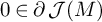 , we can thus choose
$\sigma $
, we can thus choose
$\sigma $
 in Equation (5.11) such that
$\sigma |_{\widehat W\cap U_F}\equiv 0$
in Equation (5.11) such that
$\sigma |_{\widehat W\cap U_F}\equiv 0$
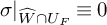 for all
$F\in {\mathcal F}^0$
for all
$F\in {\mathcal F}^0$
 . Let
$\chi \in \mathrm {C^{\infty }_c}(\widehat W)$
. Let
$\chi \in \mathrm {C^{\infty }_c}(\widehat W)$
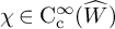 be identically equal to
$1$
be identically equal to
$1$
 on
$\overline W\setminus \bigcup _{F\in {\mathcal F}^0}U_F$
on
$\overline W\setminus \bigcup _{F\in {\mathcal F}^0}U_F$
 . Then we can extend
$\sigma $
. Then we can extend
$\sigma $
 by
$0$
by
$0$
 by setting
$\widehat \sigma :=\chi \sigma \in \Omega _{S^1}^\ast (M)$
by setting
$\widehat \sigma :=\chi \sigma \in \Omega _{S^1}^\ast (M)$
 , and
$\varrho :=\widehat \varrho -d_{\mathbf {\mathfrak g}}\widehat \sigma \in \Omega _{S^1}^\ast (M)$
, and
$\varrho :=\widehat \varrho -d_{\mathbf {\mathfrak g}}\widehat \sigma \in \Omega _{S^1}^\ast (M)$
 satisfies the properties (5.7) and (5.8). Since it differs from
$\widehat \varrho \in \Omega _{S^1}^\ast (M)$
satisfies the properties (5.7) and (5.8). Since it differs from
$\widehat \varrho \in \Omega _{S^1}^\ast (M)$
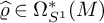 , and hence from
$\widetilde \varrho \in \Omega _{S^1}^\ast (M)$
, and hence from
$\widetilde \varrho \in \Omega _{S^1}^\ast (M)$
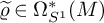 , by an equivariantly exact form,
$[\varrho ]=[\widetilde \varrho ]\in H_{S^1}^*(M)$
, by an equivariantly exact form,
$[\varrho ]=[\widetilde \varrho ]\in H_{S^1}^*(M)$
 , which concludes the proof.
Conceptually, this lemma implies that when computing the Witten integral we can make the following assumption, which will lead to substantial simplifications later.
Assumption 5.4. The equivariantly closed form
$\varrho \in \Omega _{S^1}^\ast (M)$
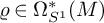 in the Witten integral (5.1) satisfies the conditions (5.7) and (5.8).
In order to obtain a meaningful geometric interpretation for the asymptotic expansion of the Witten integral, we will also make the following assumption.
Assumption 5.5. The test function
$\phi \in \mathrm {C^{\infty }_c}({\mathbb R})$
 in Definition 5.1 is identically equal to
$1$
in Definition 5.1 is identically equal to
$1$
 in a neighborhood of
$0$
in a neighborhood of
$0$
 .
.
Next, we choose a
$\delta>0$
 as in Lemma 5.3 and a cutoff function
$\tau \in \mathrm {C^{\infty }_c}({\mathbb R})$
as in Lemma 5.3 and a cutoff function
$\tau \in \mathrm {C^{\infty }_c}({\mathbb R})$
 with
$\text {supp }\tau \subset (-\delta ,\delta )$
with
$\text {supp }\tau \subset (-\delta ,\delta )$
 such that
$\tau \equiv 1$
such that
$\tau \equiv 1$
 on
$[-\delta /2,\delta /2]$
on
$[-\delta /2,\delta /2]$
 . Since
$e^{m\omega }$
. Since
$e^{m\omega }$
 is a polynomial in
$m\in {\mathbb N}$
is a polynomial in
$m\in {\mathbb N}$
 , the non-stationary phase principle implies that as
$m\to +\infty $
, the non-stationary phase principle implies that as
$m\to +\infty $
 we have for any equivariantly closed
$\varrho $
we have for any equivariantly closed
$\varrho $


so that the integral localizes around the zero level set
${ \mathcal J}^{-1}(\{0\})\subset M$
 . Now, since M is compact, we can take
$\delta $
. Now, since M is compact, we can take
$\delta $
 small enough such that with the coordinates defined by the diffeomorphisms (3.42) and (3.47) introduced in Section 3.3, we can define for every
$F\in {\mathcal F}^0$
small enough such that with the coordinates defined by the diffeomorphisms (3.42) and (3.47) introduced in Section 3.3, we can define for every
$F\in {\mathcal F}^0$
 cutoff functions
$\chi _F\in \mathrm { C^{\infty }_c}(U_F)$
cutoff functions
$\chi _F\in \mathrm { C^{\infty }_c}(U_F)$
 and
$\tau _F\in \mathrm {C^{\infty }_c}(V_F)$
and
$\tau _F\in \mathrm {C^{\infty }_c}(V_F)$
 by the characterizing relations

We then decompose the integral in (5.12) further as

We then obtain

where by pullback along
$\Phi _F$
 and thanks to Assumption 5.4 we have

5.2 Definite fixed point set components
Let us begin with the simpler case when
$0\in \partial \,{ \mathcal J}(M)$
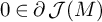 , in which case
$Q_F$
, in which case
$Q_F$
 is definite and either
$F\in {\mathcal F}^0_+$
is definite and either
$F\in {\mathcal F}^0_+$
 or
$F\in {\mathcal F}^0_-$
or
$F\in {\mathcal F}^0_-$
 . Recall also that we have
${ \mathcal J}^{-1}(\{0\})\cap U_F=F$
. Recall also that we have
${ \mathcal J}^{-1}(\{0\})\cap U_F=F$
 , which is fixed by the action of
$S^1$
, which is fixed by the action of
$S^1$
 . Pulling back the inner integral in (5.15) along the diffeomorphism
$\Psi _{F}$
. Pulling back the inner integral in (5.15) along the diffeomorphism
$\Psi _{F}$
 introduced in (3.42), taking into account Diagram (3.43) and the fact that
$\Sigma _{F\bullet }$
introduced in (3.42), taking into account Diagram (3.43) and the fact that
$\Sigma _{F\bullet }$
 has full measure in
$\Sigma _F$
has full measure in
$\Sigma _F$
 , and using (5.13) and (3.20) we get

Corollary 3.6 implies that

so that expanding the exponential series and taking into account the fact that the first and last terms of the right-hand side of (5.16) have no
$dr$
 part as they are pulled back from F and
$S_F$
part as they are pulled back from F and
$S_F$
 respectively, we get

Here we performed the change of variable
$s=m \pi r^2$
 in the last line. Note also that the infinite sum in (5.17) has only finitely many non-zero summands because
$d\Theta _{S_F}^k=0$
in the last line. Note also that the infinite sum in (5.17) has only finitely many non-zero summands because
$d\Theta _{S_F}^k=0$
 for
$k>\ell _F$
for
$k>\ell _F$
 .
.
Recall now that the Heaviside function
$H:{\mathbb R}\to {\mathbb R}$
 is defined by
$H(s)=1$
is defined by
$H(s)=1$
 for all
$s\geq 0$
for all
$s\geq 0$
 and
$H(s)=0$
and
$H(s)=0$
 otherwise. Using a standard formula for its Fourier transform as a tempered distribution [Reference Hörmander14, Example 7.1.17] and the fact that
$\tau \in \mathrm {C^{\infty }_c}({\mathbb R})$
otherwise. Using a standard formula for its Fourier transform as a tempered distribution [Reference Hörmander14, Example 7.1.17] and the fact that
$\tau \in \mathrm {C^{\infty }_c}({\mathbb R})$
 is identically equal to
$1$
is identically equal to
$1$
 on
$(-\delta /2,\delta /2)$
on
$(-\delta /2,\delta /2)$
 , one gets for any
$k\in {\mathbb N}$
, one gets for any
$k\in {\mathbb N}$
 and any Schwartz function
$\psi \in {\mathcal S}({\mathbb R})$
and any Schwartz function
$\psi \in {\mathcal S}({\mathbb R})$
 as
$m\to \infty $
as
$m\to \infty $
 the equality

where we used that
$\hat \psi $
 is rapidly decreasing and introduced the distribution
$\underline {x}^{-k}_\pm $
is rapidly decreasing and introduced the distribution
$\underline {x}^{-k}_\pm $
 defined by

which satisfies the standard relation
$\frac d {dx} \underline {x}^{-k}_\pm =-k \underline {x}^{-k-1}_\pm $
 for all
$k\in {\mathbb N}$
for all
$k\in {\mathbb N}$
 as distributions. More generally, for any absolutely converging Laurent series
$P(x)=\sum _{j=-N}^{+\infty } a_j\,x^j$
as distributions. More generally, for any absolutely converging Laurent series
$P(x)=\sum _{j=-N}^{+\infty } a_j\,x^j$
 , we will write
$P(\underline x_\pm )$
, we will write
$P(\underline x_\pm )$
 for the distribution defined by

We thus get from (5.17) that as
$m\to \infty $


Remark 5.6. Adapting the proof of Duistermaat and Heckman in [Reference Duistermaat and Heckman9, (2.11)-(2.31)] one gets from the first line of (5.21) that

where
$e_F(x)\in \Omega ^*_T(F)$
 is the equivariant Euler class of the normal bundle
${\nu _{\Sigma _F}:\Sigma _F\to F}$
is the equivariant Euler class of the normal bundle
${\nu _{\Sigma _F}:\Sigma _F\to F}$
 . Note that the integrand coincides with the integrand appearing in Berline-Vergne localization formula [Reference Berline and Vergne3], and one can actually see that our method does provide an alternative proof of it. In the application to the computation of the Riemann-Roch numbers in Section 6.1, we will not use Formula (5.22) but instead provide a direct proof based on (5.21) and the Kirillov formula of Theorem 2.10.
5.3 Indefinite fixed point set components
Let now deal with the case when we have
$0\in \operatorname {\mathrm {Int}}{ \mathcal J}(M)$
 , so that
$Q_F$
, so that
$Q_F$
 is indefinite for all
$F\in {\mathcal F}^0$
is indefinite for all
$F\in {\mathcal F}^0$
 and we have
$\ell _F^+>0$
and we have
$\ell _F^+>0$
 and
$\ell _F^->0$
and
$\ell _F^->0$
 . Using the diffeomorphism
$\Psi _{F}$
. Using the diffeomorphism
$\Psi _{F}$
 introduced in (3.47) and the coordinates (3.27), the integral (5.15) becomes

Now, by Corollary 3.7 we know that

where

is a basic form in the sense of (2.5), so that in particular
$d \bar \beta _F =d_{\mathbf {\mathfrak g}}\bar \beta _F$
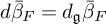 by Definition 2.1. Since

both
$\bar \beta _F$
 and
$d_{\mathbf {\mathfrak g}}\bar \beta _F$
and
$d_{\mathbf {\mathfrak g}}\bar \beta _F$
 have continuous extensions to the manifold with boundary
${S_F \times [0,\infty ) \times {\mathbb R}}$
have continuous extensions to the manifold with boundary
${S_F \times [0,\infty ) \times {\mathbb R}}$
 . On the other hand, the summand
$d\big (q\, \mathrm {pr}_{S_F}^\ast \Theta _{S_F}\big )$
. On the other hand, the summand
$d\big (q\, \mathrm {pr}_{S_F}^\ast \Theta _{S_F}\big )$
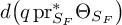 is constant with respect to r, and also the summand
$\pi _{Z_F}^\ast \mathrm {inc}_{Z_F}^\ast \omega _{\Sigma _F}$
is constant with respect to r, and also the summand
$\pi _{Z_F}^\ast \mathrm {inc}_{Z_F}^\ast \omega _{\Sigma _F}$
 extends continuously to
$r=0$
extends continuously to
$r=0$
 in view of Corollary 3.7. Inserting (5.24) into (5.23) therefore yields

where the integrals

are absolutely convergent.
5.3.1 The integral
$I_1^F(m)$


Let us first turn to the integral
$I_1^F(m)$
 . Here we closely follow the method of [Reference Meinrenken28, Proof of Theorem 3.3]. Isolating the
$dq$
. Here we closely follow the method of [Reference Meinrenken28, Proof of Theorem 3.3]. Isolating the
$dq$
 part in (5.24) and expanding the corresponding exponential series we get

Here we took Diagram (3.50) into account. Note that, as before, the infinite sums occurring here are actually finite because
$d\Theta _{S_F }^k=0$
 for
$k\in {\mathbb N}$
for
$k\in {\mathbb N}$
 large enough. Moreover, the integrand of
$\tilde I(m)$
large enough. Moreover, the integrand of
$\tilde I(m)$
 depends on the external parameters
$(p,r)\in S_F\times (0,\infty )$
depends on the external parameters
$(p,r)\in S_F\times (0,\infty )$
 only via the point
$\nu _{S_F\times (0,\infty )}(p,r)=\nu _{S_F}(p)\in F$
only via the point
$\nu _{S_F\times (0,\infty )}(p,r)=\nu _{S_F}(p)\in F$
 , so that
$\tilde I(m)$
, so that
$\tilde I(m)$
 is constant with respect to
$r\in (0,\infty )$
is constant with respect to
$r\in (0,\infty )$
 .
.
Applying the classical stationary phase principle [Reference Hörmander14, Lemma 7.7.3] to
$\tilde I(m)$
 while taking into account Assumption 5.5, we get

the estimate being uniform on
$S_F\times (0,\infty )$
 because
$S_F$
because
$S_F$
 is compact and
$\tilde I(m)$
is compact and
$\tilde I(m)$
 is constant with respect to
$r\in (0,\infty )$
is constant with respect to
$r\in (0,\infty )$
 . This yields

Here, in the second line, we consider r as a coordinate on
$Z_F$
 using the diffeomorphism
$\Psi _{F}$
using the diffeomorphism
$\Psi _{F}$
 from (3.49). The third line is obtained by pullback along the diffeomorphism
$\Phi _F^{-1}$
from (3.49). The third line is obtained by pullback along the diffeomorphism
$\Phi _F^{-1}$
 , taking into account Assumption 5.4, (3.7), the last line in Equation (5.13), and the fact that
$\chi _F$
, taking into account Assumption 5.4, (3.7), the last line in Equation (5.13), and the fact that
$\chi _F$
 is supported in
$U_F$
is supported in
$U_F$
 .
.
5.3.2 The integral
$I_2^F(m)$

Let us now turn to the integral
$ I_2^F(m)$
 . First note from (5.24) that in the coordinates (3.27) defined by the diffeomorphism (3.47), the equivariant form

is equivariantly closed. Note also that

is an equivariantly exact form. By (5.25) one concludes that

has a continuous extension to the manifold with boundary
$S_F\times [0,\infty )\times {\mathbb R}$
 . Analogously as in (4.10), consider further for
$\varepsilon \geq 0$
. Analogously as in (4.10), consider further for
$\varepsilon \geq 0$
 the manifold with boundary
$S_F \times [\varepsilon ,\infty )\times {\mathbb R}$
the manifold with boundary
$S_F \times [\varepsilon ,\infty )\times {\mathbb R}$
 , together with the canonical parametrization of its boundary given by the orientation preserving map

Using Lebesgue’s convergence theorem, Lemma 2.2, and the fact that the form (5.28) is equivariantly closed we get as
$m\to +\infty $


where we wrote

Now, analogously as in (4.12), Corollary 3.7 tells us that

Taking into account (5.30) and expanding the exponential series we therefore see that with

we obtain

Separating the sum over k into even and odd indices and using the sign function
${\mathrm {sgn}:{\mathbb R}\to {\mathbb R}}$
 defined for all
$q\in {\mathbb R}$
defined for all
$q\in {\mathbb R}$
 by
$\mathrm {sgn}(q):=H(q)-H(-q)$
by
$\mathrm {sgn}(q):=H(q)-H(-q)$
 , we rewrite
$\tilde I_2^F(m)$
, we rewrite
$\tilde I_2^F(m)$
 as
as

where we used the fact that, by the definition of
$\Theta _{S_F }$
 and
$\overline \Theta _{S_F }$
and
$\overline \Theta _{S_F }$
 in (3.46), one has

Expanding the exponential series and applying the classical stationary phase principle [Reference Hörmander14, Lemma 7.7.3] to the second term in the square bracket of (5.35) yields the asymptotic expansion

where the remainder estimate is uniform in the base point in
$S_F$
 because the latter is compact. To deal with the first term in the square bracket of (5.35) we note that with the substitution
$s=2\pi mq$
because the latter is compact. To deal with the first term in the square bracket of (5.35) we note that with the substitution
$s=2\pi mq$
 and (5.18) one computes

where we introduced the distributions

We will also use the notation (5.20) with the distributions (5.36). Expanding
$e^{m \nu _{S_F}^\ast \omega _{F}}$
 , separating powers of m, and recalling Assumption 5.5 we get from (5.35) the asymptotic expansion

up to terms of order
${\mathcal O}(m^{-\infty })$
 as
$m \to \infty $
as
$m \to \infty $
 . Let us now simplify (5.37) with the help of the binomial theorem by writing for
$x\neq 0$
. Let us now simplify (5.37) with the help of the binomial theorem by writing for
$x\neq 0$


where in the last step we used the definitions of
$\Theta _{S_F }$
 and
$\overline \Theta _{S_F }$
and
$\overline \Theta _{S_F }$
 given in (3.46). Using the exceptional Kirwan map introduced in (1.12) we finally arrive at

This deals with the first term of the right-hand side of (5.34). Using equations (5.13) and (5.28) the second term
$R_2^F(m)$
 given in (5.32) is seen to be equal to

where the basic forms
$\tilde \beta _F,\,\tilde \beta _{m,F}\in \Omega ^*(U_F\backslash F)^{S^1}_{\text {bas}}$
 are characterized by
$\Phi _F^*\tilde \beta _F:={(\Psi _F^{-1})}^*\bar \beta _F$
are characterized by
$\Phi _F^*\tilde \beta _F:={(\Psi _F^{-1})}^*\bar \beta _F$
 and
$\Phi _F^*\tilde \beta _{m,F}:={(\Psi _F^{-1})}^*\bar \beta _{m,F}$
and
$\Phi _F^*\tilde \beta _{m,F}:={(\Psi _F^{-1})}^*\bar \beta _{m,F}$
 with
$\Phi _F$
with
$\Phi _F$
 restricted to
$V_F\cap \Sigma _{F\bullet \bullet }$
restricted to
$V_F\cap \Sigma _{F\bullet \bullet }$
 ; they can be extended smoothly from
$\Phi _F(V_F\cap \Sigma _{F\bullet \bullet })$
; they can be extended smoothly from
$\Phi _F(V_F\cap \Sigma _{F\bullet \bullet })$
 to
$U_F\backslash F$
to
$U_F\backslash F$
 thanks to Formulas (5.3) and (5.30). Collecting everything we finally get

5.4 Full asymptotic expansion of the Witten integral
Let us now combine the computations of the whole section to establish the full asymptotic expansion of the Witten integral (5.1).
Theorem 5.7. Let
$\phi $
 be identically equal to
$1$
be identically equal to
$1$
 in a neighborhood of
$0$
in a neighborhood of
$0$
 . Then, for any equivariantly closed form
$\varrho \in \Omega _{S^1}^\ast (M)$
. Then, for any equivariantly closed form
$\varrho \in \Omega _{S^1}^\ast (M)$
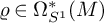 , one has the asymptotic expansion

as
$m\to +\infty $
 , where
$F\in \mathcal {F}^0_{\mathrm {exc}}$
, where
$F\in \mathcal {F}^0_{\mathrm {exc}}$
 is defined as in (1.11). Furthermore, each summand in (5.41) only depends on the equivariant cohomology class
$[\varrho ] \in H_{S^1}^*(M)$
is defined as in (1.11). Furthermore, each summand in (5.41) only depends on the equivariant cohomology class
$[\varrho ] \in H_{S^1}^*(M)$
 .
.
Proof. Let us first establish (5.41) under Assumption 5.4, assuming that
$0\in \operatorname {\mathrm {Int}}{ \mathcal J}(M)$
 . Having treated in the previous subsections all terms in (5.14) except
$\langle {\mathcal W}^{\text {reg}}_m(\varrho ),\phi \rangle $
. Having treated in the previous subsections all terms in (5.14) except
$\langle {\mathcal W}^{\text {reg}}_m(\varrho ),\phi \rangle $
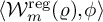 , we are left with studying the latter integral. To this end, we use the
$S^1$
, we are left with studying the latter integral. To this end, we use the
$S^1$
 -equivariant diffeomorphism
$\Phi _W:W\xrightarrow {\sim }{ \mathcal J}^{-1}(\{0\})^{\mathrm {reg}}\times (-\delta ,\delta )$
-equivariant diffeomorphism
$\Phi _W:W\xrightarrow {\sim }{ \mathcal J}^{-1}(\{0\})^{\mathrm {reg}}\times (-\delta ,\delta )$
 of Lemma 5.2, which provides the coordinate
$q:={ \mathcal J}(p)$
of Lemma 5.2, which provides the coordinate
$q:={ \mathcal J}(p)$
 on W. This coordinate coincides for all
$F\in {\mathcal F}^0$
on W. This coordinate coincides for all
$F\in {\mathcal F}^0$
 with the coordinate q of (3.27) via the diffeomorphism (3.47) when restricted to
$U_F\cap W$
with the coordinate q of (3.27) via the diffeomorphism (3.47) when restricted to
$U_F\cap W$
 . Now, following [Reference Meinrenken28, Proof of Theorem 3.3], and analogously to Equation (5.24) one has

where
$\text {inc}_0:{ \mathcal J}^{-1}(\{0\})^{\mathrm {reg}}\to M$
 is the inclusion,
$\Theta \in \Omega ^1({ \mathcal J}^{-1}(\{0\})^{\mathrm {reg}},{\mathbb R})$
is the inclusion,
$\Theta \in \Omega ^1({ \mathcal J}^{-1}(\{0\})^{\mathrm {reg}},{\mathbb R})$
 is any connection for the
$S^1$
is any connection for the
$S^1$
 -action on
${ \mathcal J}^{-1}(\{0\})^{\mathrm {reg}}$
-action on
${ \mathcal J}^{-1}(\{0\})^{\mathrm {reg}}$
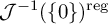 in the sense of (2.8), and
$\tilde \beta \in \Omega ^*(W)^{S^1}_{\text {bas}}$
in the sense of (2.8), and
$\tilde \beta \in \Omega ^*(W)^{S^1}_{\text {bas}}$
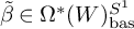 is a basic form in the sense of (2.5) satisfying
$\operatorname {{\mathrm {inc}}}_{0}^*\tilde \beta \equiv 0$
is a basic form in the sense of (2.5) satisfying
$\operatorname {{\mathrm {inc}}}_{0}^*\tilde \beta \equiv 0$
 . Furthermore, thanks to (5.4) and comparing with (5.24), we can choose the forms in (5.42) in such a way that for all
$F\in {\mathcal F}^0$
. Furthermore, thanks to (5.4) and comparing with (5.24), we can choose the forms in (5.42) in such a way that for all
$F\in {\mathcal F}^0$
 we have

with
$\Phi _F$
 suitably restricted. In the same way as in (5.29), let us write

with
$\tilde \beta _{m}\in \Omega ^*(W)^{S^1}_{\text {bas}}$
 satisfying
$\Phi _F^*(\tilde \beta _m|_{ U_F\cap W})=(\Psi _F^{-1})^*\bar \beta _{m,F}$
satisfying
$\Phi _F^*(\tilde \beta _m|_{ U_F\cap W})=(\Psi _F^{-1})^*\bar \beta _{m,F}$
 for all
$F\in {\mathcal F}^0$
for all
$F\in {\mathcal F}^0$
 . In particular, recalling the definitions of the forms appearing in (5.39), we have that
$\tilde \beta =\tilde \beta _F$
. In particular, recalling the definitions of the forms appearing in (5.39), we have that
$\tilde \beta =\tilde \beta _F$
 and
$\tilde \beta _m=\tilde \beta _{m,F}$
and
$\tilde \beta _m=\tilde \beta _{m,F}$
 on
$U_F\cap W$
on
$U_F\cap W$
 . Following [Reference Meinrenken28, Proof of Theorem 3.3], which boils down to carrying over the computations from Section 5.3 to the present situation, and using Assumption 5.4, we then readily obtain

as
$m\to +\infty $
 , with
$R_2^F(m)$
, with
$R_2^F(m)$
 as in (5.39). Inserting (5.43) into the original expression (5.14) for
$\langle {\mathcal W}_m(\varrho ),\phi \rangle $
as in (5.39). Inserting (5.43) into the original expression (5.14) for
$\langle {\mathcal W}_m(\varrho ),\phi \rangle $
 while taking into account (5.26), the first term on the right-hand side of (5.43) combines with the integrals
$I_1^F(m)$
while taking into account (5.26), the first term on the right-hand side of (5.43) combines with the integrals
$I_1^F(m)$
 computed in (5.27) in such a way that all terms involving the cutoff functions
$\chi _F$
computed in (5.27) in such a way that all terms involving the cutoff functions
$\chi _F$
 disappear. Similarly, the remainder term
$R_2^F(m)$
disappear. Similarly, the remainder term
$R_2^F(m)$
 appears in (5.43) and in (5.40) with opposite signs and thus gets cancelled out, which leaves only the term (5.38). Summing up, we get

as
$m\to +\infty $
 . If we now insert the expression (5.21) for the integrals
$\langle {\mathcal W}^{F}_m(\varrho ),\phi \rangle $
. If we now insert the expression (5.21) for the integrals
$\langle {\mathcal W}^{F}_m(\varrho ),\phi \rangle $
 with definite F and the expression (5.38) for the integrals
$\tilde I_2^F(m)$
with definite F and the expression (5.38) for the integrals
$\tilde I_2^F(m)$
 and apply Lemma 2.6 to the regular Kirwan map (4.3), we get the asymptotics (5.41) for any equivariantly closed
$\varrho \in \Omega _{S^1}^\ast (M)$
and apply Lemma 2.6 to the regular Kirwan map (4.3), we get the asymptotics (5.41) for any equivariantly closed
$\varrho \in \Omega _{S^1}^\ast (M)$
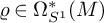 satisfying Assumption 5.4. The asymptotics (5.41) in case
$0\in \partial \,{ \mathcal J}(M)$
satisfying Assumption 5.4. The asymptotics (5.41) in case
$0\in \partial \,{ \mathcal J}(M)$
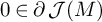 follow in the same way from the computations of Section 5.2.
Let us now deal with the case of a general equivariantly closed form
$\varrho \in \Omega _{S^1}^\ast (M)$
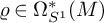 which not necessarily satisfies Assumption 5.4. First, note that thanks to Lemma 5.3 the left-hand side of (5.41) only depends on the equivariant cohomology class of
$\varrho $
which not necessarily satisfies Assumption 5.4. First, note that thanks to Lemma 5.3 the left-hand side of (5.41) only depends on the equivariant cohomology class of
$\varrho $
 . On the other hand, by the same lemma one can write
$\varrho =\tilde \varrho +d_{\mathbf {\mathfrak g}}\beta $
. On the other hand, by the same lemma one can write
$\varrho =\tilde \varrho +d_{\mathbf {\mathfrak g}}\beta $
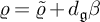 with
$\tilde \varrho \in \Omega _{S^1}^\ast (M)$
with
$\tilde \varrho \in \Omega _{S^1}^\ast (M)$
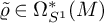 satisfying Assumption 5.4, so that we can apply (5.41) to
$ \langle {\mathcal W}_m(\varrho ),\phi \rangle = \langle {\mathcal W}_m(\tilde \varrho ),\phi \rangle $
satisfying Assumption 5.4, so that we can apply (5.41) to
$ \langle {\mathcal W}_m(\varrho ),\phi \rangle = \langle {\mathcal W}_m(\tilde \varrho ),\phi \rangle $
 . Since the equivariant homotopy Lemma 2.3 implies that we can choose
$\beta $
. Since the equivariant homotopy Lemma 2.3 implies that we can choose
$\beta $
 such that
$\beta _F:=\operatorname {{\mathrm {inc}}}_F^*\beta \equiv 0$
such that
$\beta _F:=\operatorname {{\mathrm {inc}}}_F^*\beta \equiv 0$
 , it follows from Lemma 4.5 that the first term on the right-hand side of (5.41) remains unchanged if we replace
$ \varrho $
, it follows from Lemma 4.5 that the first term on the right-hand side of (5.41) remains unchanged if we replace
$ \varrho $
 by
$\tilde \varrho $
by
$\tilde \varrho $
 ; as
$ \varrho _F=\tilde \varrho _F$
; as
$ \varrho _F=\tilde \varrho _F$
 , all other terms on the right-hand side are also unchanged, and we obtain (5.41) for
$\varrho $
, all other terms on the right-hand side are also unchanged, and we obtain (5.41) for
$\varrho $
 .
.
Finally note that Lemma 2.6, applied to the
$S^1$
 -actions on
$S_F^{\pm }$
-actions on
$S_F^{\pm }$
 in (1.9) with connections
$\Theta ^{\pm }_{S_F}$
in (1.9) with connections
$\Theta ^{\pm }_{S_F}$
 , respectively, implies that all terms on the right-hand side of (5.41), except maybe the first one, depend only on the equivariant cohomology class of
$\varrho $
, respectively, implies that all terms on the right-hand side of (5.41), except maybe the first one, depend only on the equivariant cohomology class of
$\varrho $
 . Since this is also true for the left-hand side by Lemma 5.3, this implies that the first term of the right-hand side only depends on the equivariant cohomology class of
$\varrho $
. Since this is also true for the left-hand side by Lemma 5.3, this implies that the first term of the right-hand side only depends on the equivariant cohomology class of
$\varrho $
 up to an error of
${\mathcal O}(m^{-\infty })$
up to an error of
${\mathcal O}(m^{-\infty })$
 as
$m\to +\infty $
as
$m\to +\infty $
 . But as this term is polynomial in
$m\in {\mathbb N}$
. But as this term is polynomial in
$m\in {\mathbb N}$
 , this error actually vanishes identically in
$m\in {\mathbb N}$
, this error actually vanishes identically in
$m\in {\mathbb N}$
 . This concludes the proof of the theorem.
Remark 5.8. Recalling the definition of
$S_F$
 from (3.44), we see that
$S_F=S_F^+\times _F S_F^-$
from (3.44), we see that
$S_F=S_F^+\times _F S_F^-$
 as a fiberwise product, where we set
$S_F^{\pm }:=P_F\times _{K_F}S_\pm ^{2l^{\pm }+1}$
as a fiberwise product, where we set
$S_F^{\pm }:=P_F\times _{K_F}S_\pm ^{2l^{\pm }+1}$
 . On the other hand, the
$1$
. On the other hand, the
$1$
 -forms
$\Theta _{S_F}^\pm $
-forms
$\Theta _{S_F}^\pm $
 are connections for the
$S^1$
are connections for the
$S^1$
 -actions on
$S_F^{\pm }$
-actions on
$S_F^{\pm }$
 , respectively. Thus, adapting the proof of Duistermaat and Heckman in [Reference Duistermaat and Heckman9, (2.11)-(2.31)], and using the multiplicativity of the Euler class one gets from (5.44) that as
$m\to +\infty $
, respectively. Thus, adapting the proof of Duistermaat and Heckman in [Reference Duistermaat and Heckman9, (2.11)-(2.31)], and using the multiplicativity of the Euler class one gets from (5.44) that as
$m\to +\infty $
 one has

where
$e_F(x)\in \Omega ^*_{S^1}(F)$
 is the equivariant Euler class of the normal bundle
$\nu _{\Sigma _F}:\Sigma _F\to F$
is the equivariant Euler class of the normal bundle
$\nu _{\Sigma _F}:\Sigma _F\to F$
 . Note again that the integrands in the last terms coincide with the integrand appearing in Berline-Vergne localization formula [Reference Berline and Vergne3]. As already pointed out in Remark 5.6, we will not use this fact for the computation of the Riemann-Roch numbers in the next section, but instead provide a direct proof based on (5.41) and the Kirillov formula of Theorem 2.10.
6 Invariant Riemann-Roch formula
In this section, we will proceed to the proof of our main result Theorem 1.1.
6.1 Asymptotics of Riemann-Roch numbers
In what follows, we will relate the asymptotics as
$m\to +\infty $
 of the G-invariant Riemann-Roch numbers of Definition 2.9 for
$G=S^1$
of the G-invariant Riemann-Roch numbers of Definition 2.9 for
$G=S^1$
 with the asymptotics of the Witten integral (5.1). As in Theorem 1.1, we assume that the action of
$S^1$
with the asymptotics of the Witten integral (5.1). As in Theorem 1.1, we assume that the action of
$S^1$
 is free on
${ \mathcal J}^{-1}(\{0\})\setminus M^{S^1}$
is free on
${ \mathcal J}^{-1}(\{0\})\setminus M^{S^1}$
 . Recall the identification (2.6) sending
$X\in \mathbf {\mathfrak g}$
. Recall the identification (2.6) sending
$X\in \mathbf {\mathfrak g}$
 to
$x\in {\mathbb R}$
to
$x\in {\mathbb R}$
 . We then have the following
Proposition 6.1. Under the assumptions of Theorem 1.1, there exists a neighborhood
$V_0\subset \mathbf {\mathfrak g}$
 of
$0\in \mathbf {\mathfrak g}$
of
$0\in \mathbf {\mathfrak g}$
 and a test function
$\psi \in \mathrm {C^{\infty }_c}(\exp (V_0),{\mathbb R})$
and a test function
$\psi \in \mathrm {C^{\infty }_c}(\exp (V_0),{\mathbb R})$
 which is identically equal to
$1$
which is identically equal to
$1$
 around
$e\in S^1$
around
$e\in S^1$
 such that

as
$m\to +\infty $
 , where
$\langle {\mathcal W}_{m}(\varrho ),\phi \rangle $
, where
$\langle {\mathcal W}_{m}(\varrho ),\phi \rangle $
 is the Witten integral (5.1) evaluated on
$\varrho (x):=\operatorname {\mathrm {Td}}_{\mathbf {\mathfrak g}}(M,X)\in \Omega ^*_{S^1}(M)$
is the Witten integral (5.1) evaluated on
$\varrho (x):=\operatorname {\mathrm {Td}}_{\mathbf {\mathfrak g}}(M,X)\in \Omega ^*_{S^1}(M)$
 and
$\phi \in \mathrm {C^{\infty }_c}(V_0,{\mathbb R})$
and
$\phi \in \mathrm {C^{\infty }_c}(V_0,{\mathbb R})$
 is defined by
$\phi (x):=\psi (\exp (X))\in \mathrm {C^{\infty }_c}(V_0,{\mathbb R})$
is defined by
$\phi (x):=\psi (\exp (X))\in \mathrm {C^{\infty }_c}(V_0,{\mathbb R})$
 for all
$x\in {\mathbb R}$
for all
$x\in {\mathbb R}$
 .
.
Proof. In view of the compactness of
$S^1$
 we know that there exists an
$\varepsilon>0$
we know that there exists an
$\varepsilon>0$
 and a finite subset
$\{g_0=e,g_1,\cdots , g_r\}\subset S^1$
and a finite subset
$\{g_0=e,g_1,\cdots , g_r\}\subset S^1$
 such that the Kirillov formula of Theorem 2.10 can be applied with
$g=g_j$
such that the Kirillov formula of Theorem 2.10 can be applied with
$g=g_j$
 for all
$|X|<\varepsilon $
for all
$|X|<\varepsilon $
 and all
$1\leq j\leq r$
and all
$1\leq j\leq r$
 , and such that
$\{g_j\exp (V_0)\}_{j=1}^r$
, and such that
$\{g_j\exp (V_0)\}_{j=1}^r$
 is an open cover of
$S^1$
is an open cover of
$S^1$
 , where
$V_0\simeq (-\varepsilon ,\varepsilon )\subset \mathbf {\mathfrak g}$
, where
$V_0\simeq (-\varepsilon ,\varepsilon )\subset \mathbf {\mathfrak g}$
 under the identification
$\mathbf {\mathfrak g}\simeq {\mathbb R}$
under the identification
$\mathbf {\mathfrak g}\simeq {\mathbb R}$
 of (2.6). Let
$\{\psi _j\}_{j=1}^r$
of (2.6). Let
$\{\psi _j\}_{j=1}^r$
 be an associated partition of unity, and set
$\phi _j(x):=\psi _j(\exp (X))\in \mathrm {C^{\infty }_c}(V_0,{\mathbb R})$
be an associated partition of unity, and set
$\phi _j(x):=\psi _j(\exp (X))\in \mathrm {C^{\infty }_c}(V_0,{\mathbb R})$
 for all
$x\in {\mathbb R}$
for all
$x\in {\mathbb R}$
 under the identification (2.6). We set
$\psi :=\psi _0$
under the identification (2.6). We set
$\psi :=\psi _0$
 and
$\phi :=\phi _0$
and
$\phi :=\phi _0$
 . Note also that for any
$1\leq j\leq r$
. Note also that for any
$1\leq j\leq r$
 we have
$\mathfrak {z}_{g_j}=\mathbf {\mathfrak g}$
we have
$\mathfrak {z}_{g_j}=\mathbf {\mathfrak g}$
 in Theorem 2.10 since
$S^1$
in Theorem 2.10 since
$S^1$
 is abelian. Applying Theorem 2.10 to (2.16) we get with (2.18)

To establish (6.1), we thus need to identify the second term of the right-hand side of (6.2) with the second term of the right-hand side of (6.1) up to
$O(m^{-\infty })$
 .
.
For this sake, note that by the Kostant formula (2.12) and the identification (2.6) we have on
$M^{S^1}$
 the equality

For each
$1\leq j\leq r$
 , let
$X_j\in \mathbf {\mathfrak g}$
, let
$X_j\in \mathbf {\mathfrak g}$
 be such that
$g_j=\exp (X_j)$
be such that
$g_j=\exp (X_j)$
 , and let
$x_j\in {\mathbb R}$
, and let
$x_j\in {\mathbb R}$
 be its image under the identification (2.6) sending
$X\in \mathbf {\mathfrak g}$
be its image under the identification (2.6) sending
$X\in \mathbf {\mathfrak g}$
 to
$x\in {\mathbb R}$
to
$x\in {\mathbb R}$
 . Further, for any
$1\leq j\leq r$
. Further, for any
$1\leq j\leq r$
 let us write
${\mathcal F}_j$
let us write
${\mathcal F}_j$
 for the set of connected components of
$M^{g_j}$
for the set of connected components of
$M^{g_j}$
 , and for each
$F\in {\mathcal F}_j$
, and for each
$F\in {\mathcal F}_j$
 , consider the associated isotypic decomposition as in (3.2) of its normal bundle
$\nu _{\Sigma _F}:\Sigma _F\to F$
, consider the associated isotypic decomposition as in (3.2) of its normal bundle
$\nu _{\Sigma _F}:\Sigma _F\to F$
 with respect to the induced
${S^1}$
with respect to the induced
${S^1}$
 -action. Write
$R^{\Sigma _F}=\sum _{k\in W} R^{\Sigma _F^{(k)}}$
-action. Write
$R^{\Sigma _F}=\sum _{k\in W} R^{\Sigma _F^{(k)}}$
 for the splitting of the curvature of the connection
$\nabla ^{\Sigma _F}$
for the splitting of the curvature of the connection
$\nabla ^{\Sigma _F}$
 in this decomposition. Since
$M^{S^1}\subset M^{g_j}$
in this decomposition. Since
$M^{S^1}\subset M^{g_j}$
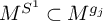 and the
$S^1$
and the
$S^1$
 -action is free on
${ \mathcal J}^{-1}(\left \{ 0 \right \})^{\text {reg}}$
-action is free on
${ \mathcal J}^{-1}(\left \{ 0 \right \})^{\text {reg}}$
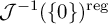 we know that
${\mathcal F}^0\subset {\mathcal F}_j$
we know that
${\mathcal F}^0\subset {\mathcal F}_j$
 , where
${\mathcal F}^0$
, where
${\mathcal F}^0$
 is as in Notation 3.1. Furthermore, by the local normal form theorem of Proposition 3.2 and the compactness of
$M^{g_j}$
is as in Notation 3.1. Furthermore, by the local normal form theorem of Proposition 3.2 and the compactness of
$M^{g_j}$
 we know that there is a
$\delta>0$
we know that there is a
$\delta>0$
 such that

Now, from (2.17) it is clear that for all
$F\in {\mathcal F}_j$
 the forms
$\operatorname {\mathrm {Td}}_{\mathbf {\mathfrak g}}(F,x)\in \Omega ^*(M)$
the forms
$\operatorname {\mathrm {Td}}_{\mathbf {\mathfrak g}}(F,x)\in \Omega ^*(M)$
 induced by the equivariant Todd class
$\operatorname {\mathrm {Td}}_{\mathbf {\mathfrak g}}(F,X)\in \Omega ^*(M)\in \Omega ^*_G(M)$
induced by the equivariant Todd class
$\operatorname {\mathrm {Td}}_{\mathbf {\mathfrak g}}(F,X)\in \Omega ^*(M)\in \Omega ^*_G(M)$
 via the identification (2.6) are smooth in
$x\in {\mathbb R}$
via the identification (2.6) are smooth in
$x\in {\mathbb R}$
 , and that for all
$F\in {\mathcal F}^0$
, and that for all
$F\in {\mathcal F}^0$
 we have
$\operatorname {\mathrm {Td}}_{\mathbf {\mathfrak g}}(F,x)=\operatorname {\mathrm {Td}}(F)$
we have
$\operatorname {\mathrm {Td}}_{\mathbf {\mathfrak g}}(F,x)=\operatorname {\mathrm {Td}}(F)$
 . Using (1.2) and the non-stationary phase principle we then get

as
$m\to +\infty $
 . Summing over all
$1\leq j\leq r$
. Summing over all
$1\leq j\leq r$
 and using that
$\sum _{j=1}^r\psi _j=1-\psi $
and using that
$\sum _{j=1}^r\psi _j=1-\psi $
 , we get that the second term of the right-hand side of (6.2) equals the second term of the right-hand side of (6.1) up to an error of size
${\mathcal O}(m^{-\infty })$
, we get that the second term of the right-hand side of (6.2) equals the second term of the right-hand side of (6.1) up to an error of size
${\mathcal O}(m^{-\infty })$
 , concluding the proof.
6.2 Proof of Theorem 1.1
We are now ready to prove Theorem 1.1 combining Proposition 6.1 with the full asymptotic expansion of the Witten integral in Theorem 5.7. The case of interest is when
$0\in \operatorname {\mathrm {Int}}{ \mathcal J}(M)$
 , so let’s treat this first. Let
$\varrho $
, so let’s treat this first. Let
$\varrho $
 and
$\phi $
and
$\phi $
 be as in the previous proposition, and take
$\tilde \psi \in \mathrm {C^{\infty }}({S^1},{\mathbb R})$
be as in the previous proposition, and take
$\tilde \psi \in \mathrm {C^{\infty }}({S^1},{\mathbb R})$
 with compact support in the small neighborhood
$U_e$
with compact support in the small neighborhood
$U_e$
 of
$e\in {S^1}$
of
$e\in {S^1}$
 , but such that
$e\notin \text {supp}\,\tilde \psi $
, but such that
$e\notin \text {supp}\,\tilde \psi $
 , and write
$\tilde \phi (x):=\tilde \psi (\exp (X))\in \mathrm { C^{\infty }_c}(V_0,{\mathbb R})$
, and write
$\tilde \phi (x):=\tilde \psi (\exp (X))\in \mathrm { C^{\infty }_c}(V_0,{\mathbb R})$
 for the induced function. Since
$\psi + \tilde \psi \in \mathrm {C^{\infty }_c}(U_e,{\mathbb R})$
for the induced function. Since
$\psi + \tilde \psi \in \mathrm {C^{\infty }_c}(U_e,{\mathbb R})$
 is identically
$1$
is identically
$1$
 close to e, Formula (6.1) also holds with the cut-off function
$\psi $
close to e, Formula (6.1) also holds with the cut-off function
$\psi $
 replaced by
$\psi + \tilde \psi $
replaced by
$\psi + \tilde \psi $
 . Therefore, taking the difference of the two resulting formulas, whose left-hand sides do not depend on the cut-off functions, Formula (5.41) applied to
$\phi +\tilde \phi $
. Therefore, taking the difference of the two resulting formulas, whose left-hand sides do not depend on the cut-off functions, Formula (5.41) applied to
$\phi +\tilde \phi $
 and
$\tilde \phi $
and
$\tilde \phi $
 implies

as
$m\to +\infty $
 , where we took into account that the singular support of the distributions appearing in (5.41) is given by
$\{0\}\subset {\mathbb R}$
, where we took into account that the singular support of the distributions appearing in (5.41) is given by
$\{0\}\subset {\mathbb R}$
 , so that they turn into regular integrals over
${\mathbb R}$
, so that they turn into regular integrals over
${\mathbb R}$
 as
$0\notin \operatorname {\mbox {supp }}\tilde \phi $
as
$0\notin \operatorname {\mbox {supp }}\tilde \phi $
 by assumption. Now, as (6.4) holds for all test functions
$\tilde \psi \in \mathrm {C^{\infty }_c}({U_e\setminus \{e\}},{\mathbb R})$
by assumption. Now, as (6.4) holds for all test functions
$\tilde \psi \in \mathrm {C^{\infty }_c}({U_e\setminus \{e\}},{\mathbb R})$
 , one deduces from this for
$x\neq 0$
, one deduces from this for
$x\neq 0$
 the identity of Laurent polynomials

since both sides are polynomials in
$m\in {\mathbb N}$
 , so that the error term
${\mathcal O}(m^{-\infty })$
, so that the error term
${\mathcal O}(m^{-\infty })$
 vanishes. Comparing this with the full asymptotic expansion of the Witten integral (5.41) and using the notation introduced in (5.20), this implies

Plugging this into Proposition 6.1 and expressing the distributions (5.19) and (5.36) as distributions on the Lie group
${S^1}$
 we get

where
$\widetilde {\chi }^{(m)}_F$
 is the meromorphic function defined for any
$F\in {\mathcal F}^0$
is the meromorphic function defined for any
$F\in {\mathcal F}^0$
 and
$z\in {\mathbb C}$
and
$z\in {\mathbb C}$
 by
by

Notice that the dependence on the test function
$\psi $
 has cancelled out in (6.5). Now, by a result of Meinrenken in [Reference Meinrenken28, Theorem 5.1], the left-hand side of (6.5) is an arithmetic polynomial in
$m\in {\mathbb N}$
has cancelled out in (6.5). Now, by a result of Meinrenken in [Reference Meinrenken28, Theorem 5.1], the left-hand side of (6.5) is an arithmetic polynomial in
$m\in {\mathbb N}$
 , while the terms of the right-hand side except
${\mathcal O}(m^{-\infty })$
, while the terms of the right-hand side except
${\mathcal O}(m^{-\infty })$
 are polynomials in
$m\in {\mathbb N}$
are polynomials in
$m\in {\mathbb N}$
 , so that the error term in (6.5) actually vanishes identically in
$m\in {\mathbb N}$
, so that the error term in (6.5) actually vanishes identically in
$m\in {\mathbb N}$
 .
.
Note that, as seen for instance from [Reference Duistermaat, Guillemin, Meinrenken and Wu8, (2.5)], the poles of
$\widetilde {\chi }^{(m)}_F(z)$
 are contained in
$\{0,1\}\subset {\mathbb C}$
are contained in
$\{0,1\}\subset {\mathbb C}$
 . Therefore, with a change of coordinates the residue theorem implies that

Using a change of variable
$z\mapsto z^{-1}$
 we get in the same way

Inserting this in (6.5) and taking
$m=1$
 then finally yields (1.10) in case that
$0\in \operatorname {\mathrm {Int}}{ \mathcal J}(M)$
then finally yields (1.10) in case that
$0\in \operatorname {\mathrm {Int}}{ \mathcal J}(M)$
 . The case
$0\in \partial \,{ \mathcal J}(M)$
. The case
$0\in \partial \,{ \mathcal J}(M)$
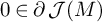 follows in a completely analogous way and reduces to the original proof of Duistermaat, Guillemin, Meinrenken, and Wu in [Reference Duistermaat, Guillemin, Meinrenken and Wu8, § 2].
Remark 6.2. Note that Formula (6.4) can also be obtained from the formula for the Witten integral given in Remark 5.8 by using the explicit Formula (2.17) for the equivariant Todd class and the explicit formula for the equivariant Euler class following for instance [Reference Berline, Getzler and Vergne2, § 8.1]. This fact is actually at the basis of the deduction of the Kirillov formula of Theorem 2.10 from the equivariant index theorem (2.21). In the definite setting of Section 5.2, our method actually gives an alternative proof of this fact, using the theory of distributions instead of the standard methods of equivariant cohomology.
6.3 Examples
Let us close by illustrating Theorem 1.1 through a family of examples. Fix an m-tuple
$(k_1,\cdots , k_m)\in {\mathbb Z}^m$
 with
$m\in {\mathbb N}$
with
$m\in {\mathbb N}$
 . We consider the product
$M=\Pi _{j=1}^m S^2$
. We consider the product
$M=\Pi _{j=1}^m S^2$
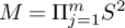 of
$m$
of
$m$
 copies of the
$2$
copies of the
$2$
 -sphere
$S^2$
-sphere
$S^2$
 endowed with the symplectic form
$\omega $
endowed with the symplectic form
$\omega $
 whose pullback to each
$S^2$
whose pullback to each
$S^2$
 -factor is the standard volume form of volume
$1$
-factor is the standard volume form of volume
$1$
 . We regard M as equipped with the diagonal
$S^1$
. We regard M as equipped with the diagonal
$S^1$
 -action such that
$\phi \in {\mathbb R}/{\mathbb Z}\simeq S^1$
-action such that
$\phi \in {\mathbb R}/{\mathbb Z}\simeq S^1$
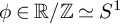 acts on the j-th sphere by a rotation of angle
$2\pi k_j\phi $
acts on the j-th sphere by a rotation of angle
$2\pi k_j\phi $
 around the z-axis of
$S^2\subset {\mathbb R}^3$
around the z-axis of
$S^2\subset {\mathbb R}^3$
 . This action is Hamiltonian for the moment map

where for any
$k\in {\mathbb Z}$
 , the map
${ \mathcal J}_k:S^2\to {\mathbb R}$
, the map
${ \mathcal J}_k:S^2\to {\mathbb R}$
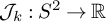 denotes the moment map associated with the
$S^1$
denotes the moment map associated with the
$S^1$
 -action of weight k, which is explicitly given by
${ \mathcal J}_k(x,y,z)=kz$
-action of weight k, which is explicitly given by
${ \mathcal J}_k(x,y,z)=kz$
 in the Euclidean coordinates
$x,y,z$
in the Euclidean coordinates
$x,y,z$
 of
${\mathbb R}^3\supset S^2$
of
${\mathbb R}^3\supset S^2$
 . The connected components of the fixed point set
$M^{S^1}$
. The connected components of the fixed point set
$M^{S^1}$
 are all isolated points, given by products of north and south poles, and the constant term subtracted in (6.7) ensures that at least the product of all north poles (where
$z=1$
are all isolated points, given by products of north and south poles, and the constant term subtracted in (6.7) ensures that at least the product of all north poles (where
$z=1$
 ) is contained in
${ \mathcal J}^{-1}(\{0\})$
) is contained in
${ \mathcal J}^{-1}(\{0\})$
 , with weights counted with multiplicity given by
$(k_1,\ldots , k_m)\in {\mathbb Z}^m$
, with weights counted with multiplicity given by
$(k_1,\ldots , k_m)\in {\mathbb Z}^m$
 . This shows in particular that any given set of weights
$W\subset {\mathbb Z}$
. This shows in particular that any given set of weights
$W\subset {\mathbb Z}$
 with any multiplicities can occur. Theorem 1.1 then provides an explicitly computable formula for the
$S^1$
with any multiplicities can occur. Theorem 1.1 then provides an explicitly computable formula for the
$S^1$
 -invariant Riemann-Roch numbers
$RR(M,L)^{S^1}$
-invariant Riemann-Roch numbers
$RR(M,L)^{S^1}$
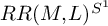 , and under the combinatorial condition (4.17) the regular term can be expressed in terms of characteristic classes involving only the topology of the resolution
$\widetilde {\mathscr M}_0$
, and under the combinatorial condition (4.17) the regular term can be expressed in terms of characteristic classes involving only the topology of the resolution
$\widetilde {\mathscr M}_0$
 .
.
In the particular case of
$M=S^2\times S^2$
 with weights
$k_1=-1$
with weights
$k_1=-1$
 and
$k_2=1$
and
$k_2=1$
 , the partial resolution
$\widetilde {\mathscr M}_0$
, the partial resolution
$\widetilde {\mathscr M}_0$
 is diffeomorphic to
$S^2$
is diffeomorphic to
$S^2$
 , and the quotient map
$\widetilde Z\to \widetilde {\mathscr M}_0$
, and the quotient map
$\widetilde Z\to \widetilde {\mathscr M}_0$
 is a trivial
$S^1$
is a trivial
$S^1$
 -principal bundle. One then checks that we recover the usual Riemann-Roch formula for the sphere
$S^2$
-principal bundle. One then checks that we recover the usual Riemann-Roch formula for the sphere
$S^2$
 as the right-hand side of (1.10), and that the second and third terms of the right-hand side of Formula (1.10) vanish, so that Formula (1.10) reads
$RR(S^2\times S^2,L^m\boxtimes L^m)^{S^1}=RR(S^2,L^m)$
as the right-hand side of (1.10), and that the second and third terms of the right-hand side of Formula (1.10) vanish, so that Formula (1.10) reads
$RR(S^2\times S^2,L^m\boxtimes L^m)^{S^1}=RR(S^2,L^m)$
 for all
$m\in {\mathbb N}$
for all
$m\in {\mathbb N}$
 and L the prequantizing line bundle of
$(S^2,\omega )$
and L the prequantizing line bundle of
$(S^2,\omega )$
 , as one can easily compute explicitly.
Acknowledgement
We would like to thank Michèle Vergne for her continuous interest in our work and her encouragement, and Paul-Emile Paradan for stimulating discussions. The first author has received funding from the Deutsche Forschungsgemeinschaft (DFG, German Research Foundation) – Project-ID 491392403 – TRR 358 and through the Priority Program (SPP) 2026 ‘Geometry at Infinity’, while the second author was partially supported by the Alexander von Humboldt Stiftung (Alexander von Humboldt Foundation) and by ANR-23-CE40-0021-01 JCJC project QCM. Finally, we thank an anonymous referee for suggesting several improvements.
Competing interests
The authors have no competing interests to declare.
Data availability statement
None.


 Open access

