





The performance in a test does not only reflect a test taker’s level of capability, but also his motivation to do well (Knekta, Reference Knekta2017). When test takers have little motivation to take a test, they tend to respond prematurely in order to avoid mental work as soon as test items become harder (Debeer et al., Reference Debeer, Buchholz, Hartig and Janssen2014; Wise & Smith, Reference Wise, Smith, Bovaird, Geisinger and Buckendal2011). This results in an overestimation of the item difficulties, an underestimation of the average capability level of the test takers, and threatens the validity of the test when the test scores are interpreted in terms of capability solely (Oshima, Reference Oshima1994; Rios, Reference Rios2022; van Laar & Braeken, Reference van Laar and Braeken2022).
Premature responses are often conceived as rapid guesses (Wise, Reference Wise2017). Rapid guesses are fast responses based on an incomplete response process that does not reflect the capability of a test taker (Wise & DeMars, Reference Wise and DeMars2006). Rapid guesses are typically accounted for by mixture models that assume two qualitatively different modes of responding (dual-process assumption).Footnote 1 In the first response mode, a test taker employs his capabilities and responds in a regular way, engaging with the content of the item. Such regular responses are modeled by an item response model. In the second response mode, the test taker does not employ his capabilities and responds without any serious effort by a guess on chance level. Several mixture models for rapid guessing have been proposed in the past. In some models, all responses of a rapid guesser are rapid guesses (Liu et al., Reference Liu, Cheng and Liu2020; Meyer, Reference Meyer2010), while in others, it is just a subset (Wang & Xu, Reference Wang and Xu2015). Some models consider solely responses (Bolt et al., Reference Bolt, Cohen and Wollack2002; Boughton & Yamamoto, Reference Boughton, Yamamoto, Davier and Carstensen2007), some solely the response times (Schnipke & Scrams, Reference Schnipke and Scrams1997), and some responses and response times (Alós-Ferrer, Reference Alós-Ferrer2018; Molenaar et al., Reference Molenaar, Bolsinova and Vermunt2018). In some models, the likelihood of rapid guesses depends on the test taker (Lu et al., Reference Lu, Wang, Zhang and Tao2020), in some on the item (Wang & Xu, Reference Wang and Xu2015), and in some on both (Ulitzsch et al., Reference Ulitzsch, von Davier and Pohl2019).
Alternatively, the phenomenon of premature responding can be interpreted as an incomplete response process, whereby the regular response process is interrupted when it exceeds the time a test taker is willing to invest into an item. This can be modeled with race models that assume a race between the response process and a process of disengagement. In the race models, a regular response is given when the response process is completed before disengagement occurs, whereas a premature response is given when the process of disengagement wins. Measurement models based on a race have been proposed by Guo et al. (Reference Guo, Xu, Fang, Ying and Zhang2025), Lee and Ying (Reference Lee and Ying2015), Lu and Wang (Reference Lu and Wang2020), Ranger and Kuhn (Reference Ranger and Kuhn2014), and Ranger et al. (Reference Ranger, Much, Neek, Mutak and Pohl2025); see also Glickman et al. (Reference Glickman, Gray and Morales2005) and Hawkins and Heathcote (Reference Hawkins and Heathcote2021) for the application of race models in experimental psychology. The race models differ in their assumptions about the race and its consequences. In some models, the regular response is always correct (Ranger & Kuhn, Reference Ranger and Kuhn2014), while in others, the regular response is modeled by an item response model (Guo et al., Reference Guo, Xu, Fang, Ying and Zhang2025; Lee & Ying, Reference Lee and Ying2015; Lu & Wang, Reference Lu and Wang2020). In some models, the premature response is a wrong response (Lee & Ying, Reference Lee and Ying2015; Ranger & Kuhn, Reference Ranger and Kuhn2014), a guess (Ranger et al., Reference Ranger, Much, Neek, Mutak and Pohl2025), or an omission (Guo et al., Reference Guo, Xu, Fang, Ying and Zhang2025; Lu & Wang, Reference Lu and Wang2020). The models also differ in their distributional assumptions about the response process and the process of disengagement.
Mixture models and race models have been used successfully in psychological and educational assessment. However, they rely on a simplified view of the process that produces premature responses. The models allow for individual differences in the frequency of premature responses either by allowing for individual differences in the mixing proportion or the willingness to invest time. The response process underlying the premature responses, however, does not depend on characteristics of the test takers or the time on the task as premature responses are either wrong responses, omissions, or random guesses; but see the model of Ranger et al. (Reference Ranger, Much, Neek, Mutak and Pohl2025) for an exception. Guesses are rarely entirely random (Burton, Reference Burton2002; Noventa et al., Reference Noventa, Heller and Kelava2024). Even though the response process was incomplete, the test takers might still have partial knowledge that could be used for an informed guess, either by a comparative evaluation of the response options or an elimination of distractors (Gonthier, Reference Gonthier2023; Lau et al., Reference Lau, Lau, Hong and Usop2011; Weber et al., Reference Weber, Krieger, Spinath, Greiff, Hissbach and Becker2023). Mixture and race models thus capture only an extreme form of premature responding—one in which test takers either lack any relevant information or disregard the information when responding.
In this article, we propose a latent trait model for the responses and the response times on a test with a single-choice format. The model accounts for premature responses based on a race between an information accumulation process and a process of disengagement. The information accumulation process is modeled by a diffusion-based item response theory (diffIRT) model (Molenaar et al., Reference Molenaar, Tuerlinckx and van der Maas2015; Tuerlinckx et al., Reference Tuerlinckx, Molenaar, van der Maas, Linden and Hambleton2016; van der Maas et al., Reference van der Maas, Molenaar, Maris, Kievit and Borsboom2011). We propose two versions of the model. In the first version, premature responses are random guesses. In a second version, the premature responses are informed by the accumulated information. The proposed model makes several contributions. In contrast to the mixture and race models reviewed above, the model allows for estimating item- and person-specific parameters related to the disengagement process, which may serve as indicators of test-taking engagement. The model also accomodates how the guessing process depends on test taker characteristics and the time spent on task. In contrast to the race model of Ranger et al. (Reference Ranger, Much, Neek, Mutak and Pohl2025), the model incorporates within-trial noise in evidence accumulation and does not predict responses and response times deterministically from trial-wise parameters (Kang et al., Reference Kang, Molenaar and Ratcliff2023). Moreover, the diffusion model allows for a more detailed description of test-taking engagement than race model of Ranger et al. (Reference Ranger, Much, Neek, Mutak and Pohl2025) by considering the response caution of a test taker. Finally, the proposed model is an alternative to the mixture-based diffusion model introduced by Alós-Ferrer, (Reference Alós-Ferrer2018).
The outline of this manuscript is as follows. First, we describe the model in detail. Then, we investigate whether the values of the item parameters and the latent traits can be recovered by means of a simulation study. Finally, we illustrate the application of the model with two empirical examples.
1 The extended diffIRT model
The proposed model builds on the diffusion model that is first extended by a censoring process to account for prematurely responding and then embedded within a hierarchical framework to account for individual differences among test takers. We first review the diffusion model, then describe its extension by the censoring process, and finally address its integration into a hierarchical model.
1.1 The diffusion model
The diffusion model was originally developed in experimental psychology for binary decision tasks (Ratcliff, Reference Ratcliff1978), but has been used lately for responses and response times from psychological tests (Kang et al., Reference Kang, de Boeck and Ratcliff2022; Tuerlinckx & De Boeck, Reference Tuerlinckx and De Boeck2005; Tuerlinckx et al., Reference Tuerlinckx, Molenaar, van der Maas, Linden and Hambleton2016; van der Maas et al., Reference van der Maas, Molenaar, Maris, Kievit and Borsboom2011). In these applications, the response is interpreted as a binary decision between the correct and an incorrect response. The diffusion model is based on an information accumulation process. The momentary level of information at time t is represented by the random variable $X(t)$
(
$X(t)$
( $X(t) \in \mathbb {R}$
). It may be interpreted as the relative evidence in favor of the correct (
$X(t) \in \mathbb {R}$
). It may be interpreted as the relative evidence in favor of the correct ( $X(t)>0$
) or an incorrect response (
$X(t)>0$
) or an incorrect response ( $X(t)<0$
). In the unbiased version of the diffusion model, the test takers start without information (
$X(t)<0$
). In the unbiased version of the diffusion model, the test takers start without information ( $X(t=0)=0$
). The change in
$X(t=0)=0$
). The change in $X(t)$
over time is characterized by the stochastic differential equation of a Wiener process with drift
$X(t)$
over time is characterized by the stochastic differential equation of a Wiener process with drift
 $$ \begin{align} dX ( t ) = v \cdot dt + dB( t ) {,} \end{align} $$
where v is the drift rate and $dB(t)$
is a Brownian increment. The drift rate determines the expected level of information at point of time t via the relation
$dB(t)$
is a Brownian increment. The drift rate determines the expected level of information at point of time t via the relation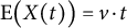 $\text {E}\big ( X(t) \big ) = v \cdot t $
. The Brownian increment represents noise and generates deviations of the actual level from the expected level of information. Its variability is determined by a parameter that is usually fixed to a specific value for the sake of model identification.
$\text {E}\big ( X(t) \big ) = v \cdot t $
. The Brownian increment represents noise and generates deviations of the actual level from the expected level of information. Its variability is determined by a parameter that is usually fixed to a specific value for the sake of model identification.
Test takers accumulate information until the momentary level of information $X(t)$
hits either an upper or a lower boundary. In case the upper boundary is hit, the test taker selects the correct response. In the other case, an incorrect response is selected. Upper and lower boundaries are denoted as
$X(t)$
hits either an upper or a lower boundary. In case the upper boundary is hit, the test taker selects the correct response. In the other case, an incorrect response is selected. Upper and lower boundaries are denoted as $a_C$
(
$a_C$
( $a_C \in \mathbb {R}^+$
) and
$a_C \in \mathbb {R}^+$
) and $a_I$
(
$a_I$
( $a_I \in \mathbb {R}^-$
) in the following. The time required to select a response is the first hitting time. In practice, the processing response time is longer than the first hitting time. Some extra time is required for reading the item or giving the response. This extra time is denominated as the non-decision time d (
$a_I \in \mathbb {R}^-$
) in the following. The time required to select a response is the first hitting time. In practice, the processing response time is longer than the first hitting time. Some extra time is required for reading the item or giving the response. This extra time is denominated as the non-decision time d ( $d \in \mathbb {R}^+$
). The processing time is the sum of the non-decision time and the first hitting time.
$d \in \mathbb {R}^+$
). The processing time is the sum of the non-decision time and the first hitting time.
An illustration of the response process is given in Figure 1, left plot (diffusion model). The straight black line represents the expected level of information of a test taker with drift rate $v=1$
as a function of time. The saw-toothed line represents the actual level of information
$v=1$
as a function of time. The saw-toothed line represents the actual level of information $X(t)$
. The actual level deviates from the expected level due to the Brownian increment. The diffusion process starts with a delay of
$X(t)$
. The actual level deviates from the expected level due to the Brownian increment. The diffusion process starts with a delay of $d=0.5$
time units. It requires
$d=0.5$
time units. It requires $t^*=1.5$
time units in order to hit a boundary for the first time. As the upper boundary
$t^*=1.5$
time units in order to hit a boundary for the first time. As the upper boundary $a_C=2$
is hit, the evidence for the correct response outweighs the evidence for the incorrect response and the test taker selects the correct response. The processing time is the non-decision time plus the first hitting time
$a_C=2$
is hit, the evidence for the correct response outweighs the evidence for the incorrect response and the test taker selects the correct response. The processing time is the non-decision time plus the first hitting time $t=t^* + d = 1.5+0.5=2.0$
. In Figure 1, the non-decision time delays the start of the information accumulation process, rather than constituting the post-decision phase of giving the response. We consider this more plausible in psychological assessment as reading an item requires considerably more time than the physical act of responding.Footnote
2
$t=t^* + d = 1.5+0.5=2.0$
. In Figure 1, the non-decision time delays the start of the information accumulation process, rather than constituting the post-decision phase of giving the response. We consider this more plausible in psychological assessment as reading an item requires considerably more time than the physical act of responding.Footnote
2
Illustration of the response process implied by the diffusion model (left plot) and the extended diffusion model with censoring (right plot). The straight black line represents the expected level of information for a test taker with drift rate $v=1$
and non-decision time
$v=1$
and non-decision time $d=0.5$
. The saw-tooth line represents the actual level of information of a test taker. Boundaries are denoted by
$d=0.5$
. The saw-tooth line represents the actual level of information of a test taker. Boundaries are denoted by $a_C$
and
$a_C$
and $a_I$
. The censoring time is represented by c.
$a_I$
. The censoring time is represented by c.

In the following, we assume that the thresholds are located symmetrically around zero ( $a_I=-a_C$
). This avoids bias in the response process and is plausible in case test takers do not have prior knowledge of which of the response options is correct (Cizek & Wollack, Reference Cizek, Wollack, Cizek and Wollack2017). When boundaries are symmetric, the diffusion process can be parameterized in terms of two parameters, the drift rate v and the boundary separation
$a_I=-a_C$
). This avoids bias in the response process and is plausible in case test takers do not have prior knowledge of which of the response options is correct (Cizek & Wollack, Reference Cizek, Wollack, Cizek and Wollack2017). When boundaries are symmetric, the diffusion process can be parameterized in terms of two parameters, the drift rate v and the boundary separation $a=a_C-a_I$
(
$a=a_C-a_I$
( $a \in \mathbb {R}^+$
).Footnote
3
Both parameters characterize different aspects of the information accumulation process. The drift rate determines the expectation of the accumulated information. It represents the information processing capability of a test taker. Test takers with high levels of v tend to give correct responses fast. The boundary separation a is related to the level of information that is required for the test taker to respond. As test takers with high levels of a tend to respond slowly, but correctly, a is interpreted as the response caution of a test taker (Boehm et al., Reference Boehm, Marsman, van der Maas and Maris2021). The non-decision time is a shift parameter that is usually not considered as a parameter pertaining to the information accumulation process.
$a \in \mathbb {R}^+$
).Footnote
3
Both parameters characterize different aspects of the information accumulation process. The drift rate determines the expectation of the accumulated information. It represents the information processing capability of a test taker. Test takers with high levels of v tend to give correct responses fast. The boundary separation a is related to the level of information that is required for the test taker to respond. As test takers with high levels of a tend to respond slowly, but correctly, a is interpreted as the response caution of a test taker (Boehm et al., Reference Boehm, Marsman, van der Maas and Maris2021). The non-decision time is a shift parameter that is usually not considered as a parameter pertaining to the information accumulation process.
The diffusion model was originally proposed for binary responses. The model can be applied to single-choice tasks in case all incorrect response options are grouped. This requires the assumption that the diffusion process reflects the comparison of the correct response with the most attractive incorrect response option. The assumption is, for example, reasonable in case all incorrect response options are roughly equally attractive (Boehm et al., Reference Boehm, Marsman, van der Maas and Maris2021). Alternatively, the diffusion model can be adapted to items with single-choice format (van der Maas et al., Reference van der Maas, Molenaar, Maris, Kievit and Borsboom2011) or can be used in order to model response-specific information accumulation (Tillman et al., Reference Tillman, Van Zandt and Logan2020), but this requires further extensions.
1.2 The extension of the diffusion model by a censoring process
The time a test taker is willing to spend on the items is an important aspect of test-taking engagement that is closely related to the tendency to respond prematurely (Baumert & Demmerich, Reference Baumert and Demmerich2001; Eklöf, Reference Eklöf2010; Knekta, Reference Knekta2017). In the diffusion model, there is no direct counterpart to the willingness to invest time. Motivational aspects of test-taking are represented by the boundary separation. The boundary separation, however, is conceptually different to the time a test taker is willing to invest. It primarily reflects the aspired level of information that might not be reached in case information accumulation is slow and test takers give up. The boundary separation is also no substitute for the willingness to invest time pragmatically as it is indeed related to the expected response time, but does not limit the actual time on the task.
We propose an extension of the diffusion model in order to account for the willingness to invest time. In the extension, we assume that each test taker sets a censoring time c. The censoring time c is the maximal time, a test taker would spend on an item. The censoring time censors the response process as follows. In case the time required to select the response (first hitting time of the diffusion process plus the non-decision time) does not exceed the censoring time, the response process is ended regularly and the response is generated by the diffusion model. Otherwise, the response process is interrupted prematurely at the censoring time c. Premature responses are generated according to two alternative procedures. In the first version of the model, we assume that the response is randomly selected among the available response options. The correct response is selected with the fixed guessing probability $\pi $
. The momentary level of information
$\pi $
. The momentary level of information $X(c)$
has no impact on the selection as it is completely ignored. In the second version of the model, the test taker responds based on the information that was accumulated until the interruption. In case the level of the accumulated information is positive (
$X(c)$
has no impact on the selection as it is completely ignored. In the second version of the model, the test taker responds based on the information that was accumulated until the interruption. In case the level of the accumulated information is positive ( $X(c)>0$
), the test taker selects the correct response. Otherwise, the test taker selects the incorrect response. Note that only the sign of
$X(c)>0$
), the test taker selects the correct response. Otherwise, the test taker selects the incorrect response. Note that only the sign of $X(c)$
matters, not the absolute value
$X(c)$
matters, not the absolute value $|X(c)|$
. Due to the randomness in
$|X(c)|$
. Due to the randomness in $X(c)$
, the model implies that responses are fast and almost on chance level when the censoring time is short. To account for the randomness in the process of disengagement, we assume that the censoring time c is the realization of a log-normally distributed random variable with scale parameter
$X(c)$
, the model implies that responses are fast and almost on chance level when the censoring time is short. To account for the randomness in the process of disengagement, we assume that the censoring time c is the realization of a log-normally distributed random variable with scale parameter $\mu $
and shape parameter
$\mu $
and shape parameter $\sigma $
. The parameters of the log-normal distribution determine the expected censoring time and will later be related to characteristics of the test taker and the item.
$\sigma $
. The parameters of the log-normal distribution determine the expected censoring time and will later be related to characteristics of the test taker and the item.
An illustration of the response process is given in Figure 1, right plot (extended diffusion model). The plot depicts the accumulated information of two test takers. Both test takers are willing to spend at most $c=2.25$
time units on the item. This is the maximal time the delayed process of information accumulation is allowed to last. One of the test takers manages to finish the response process regularly within the time limit by hitting the upper boundary at
$c=2.25$
time units on the item. This is the maximal time the delayed process of information accumulation is allowed to last. One of the test takers manages to finish the response process regularly within the time limit by hitting the upper boundary at $t=2.00$
. This test taker responds after
$t=2.00$
. This test taker responds after $t=2.00$
time units correctly. The other test taker gives up and stops information accumulation at
$t=2.00$
time units correctly. The other test taker gives up and stops information accumulation at $c=2.25$
. In the first version of the model, the test taker would guess randomly. In the second version of the model, the test taker would choose the more plausible response. As the accumulated information at
$c=2.25$
. In the first version of the model, the test taker would guess randomly. In the second version of the model, the test taker would choose the more plausible response. As the accumulated information at $c=2.25$
time units is positive, the test taker would respond correctly after
$c=2.25$
time units is positive, the test taker would respond correctly after $t=2.25$
time units.
$t=2.25$
time units.
In the second version of the extended diffusion model, the premature responses depend on partial knowledge as premature responses are determined by the sign of the accumulator when the response process is interrupted (sign rule). This response process has some resemblance to the interrogation paradigm (Bogacz et al., Reference Bogacz, Brown, Moehlis, Holmes and Cohen2006). In the interrogation paradigm, the test takers are obliged to respond at a fixed point of time. This fixed point of time, however, is set by the experimenter while in our model, the censoring time is a random variable depending on characteristics of the test taker. Furthermore, in the interrogation paradigm, the test takers are supposed to accumulate information until they are allowed to respond by the experimenter, while in our model, the test takers may respond earlier. Selecting a response based on the sign guarantees that the more likely response is selected (Bogacz et al., Reference Bogacz, Brown, Moehlis, Holmes and Cohen2006). The sign rule can also be justified on psychological grounds. In the diffusion model, the accumulator represents the impression that one response option is more plausible than the other (Fehr & Rangel, Reference Fehr and Rangel2011), the net evidence in favor of one alternative against the other (Baldassi et al., Reference Baldassi, Cerreia-Vioglio, Maccheroni, Marinacci and Pirazzini2020) or the balance of the support for the two alternatives (Kvam, Reference Kvam2019). It can be interpreted as the difference between two accumulators representing evidence for each response option (Webb, Reference Webb2019). The decision rule is relative as a response is given as soon as the evidence for one alternative over the other exceeds a threshold. Even when this threshold is not reached, as it happens when the process of information accumulation is interrupted, the relative decision rule still requires that the alternative with more net evidence (as indicated by the sign of the accumulator) is chosen. This response mechanism is different to the one in the model of Ranger et al. (Reference Ranger, Much, Neek, Mutak and Pohl2025). There, the premature responses were informed guesses with the guessing probability depending on the actual level of the accumulator. We consider this implementation to be inadequate for the diffusion model for two reasons. First, in the model of Ranger et al. (Reference Ranger, Much, Neek, Mutak and Pohl2025), the accumulator represents the actual progress toward the solution, not the relative evidence. Some progress might enable test takers to eliminate distractors, thereby increasing the guessing probability over chance level. Second, the accumulator in the diffusion model is supposed to fully characterize the response process. In case the interruption would trigger a random guess based on the actual level of the accumulator, the same level could result into different responses. Hence, there have to be differences in the knowledge state that are not fully captured by the accumulator and would require a random mechanism beyond the Brownian motion.
1.3 A hierarchical extension of the diffusion model with censoring
The parameters of the extended diffusion model are related to latent traits and item effects via a hierarchical model in order to account for differences between test takers and items. Denote by $v_{ij}$
the drift rate and by
$v_{ij}$
the drift rate and by $a_{ij}$
the boundary separation of test taker i (
$a_{ij}$
the boundary separation of test taker i ( $i=1,\ldots ,N$
) on item j (
$i=1,\ldots ,N$
) on item j ( $j=1,\ldots ,J$
) of a test. We relate the drift rate via a linear model to a first trait
$j=1,\ldots ,J$
) of a test. We relate the drift rate via a linear model to a first trait $\theta _i$
and the boundary separation via a transformed linear model to a second trait
$\theta _i$
and the boundary separation via a transformed linear model to a second trait $\omega _i$
:
$\omega _i$
:
 $$ \begin{align} v_{ij} &= v_j\big( \theta_i \big) = v_{0j} + v_{1j} \theta_i \\ a_{ij} &= a_j\big( \omega_i \big) = \log \big( 1 + \exp( a_{0j} + a_{1j} \omega_i ) \big). \notag \end{align} $$
In Equation (2), the latent traits $\theta _i$
(
$\theta _i$
( $\theta \in \mathbb {R}$
) and
$\theta \in \mathbb {R}$
) and $\omega _i$
(
$\omega _i$
( $\omega \in \mathbb {R}$
) are the capability and the response caution of test taker i, respectively. The capability comes close to what Thurstone (Reference Thurstone1937) called the power of a test taker and is usually the target trait of the assessment. The response caution has a close resemblance to the effort that is needed for a successful termination of the problem-solving process in the theory of test-taking motivation of Knekta (Reference Knekta2017) and represents the aspiration level of a test taker. The item parameters
$\omega \in \mathbb {R}$
) are the capability and the response caution of test taker i, respectively. The capability comes close to what Thurstone (Reference Thurstone1937) called the power of a test taker and is usually the target trait of the assessment. The response caution has a close resemblance to the effort that is needed for a successful termination of the problem-solving process in the theory of test-taking motivation of Knekta (Reference Knekta2017) and represents the aspiration level of a test taker. The item parameters $v_{0j}$
(
$v_{0j}$
( $v_{0j} \in \mathbb {R}$
) and
$v_{0j} \in \mathbb {R}$
) and $a_{0j}$
(
$a_{0j}$
( $a_{0j} \in \mathbb {R}$
) determine the drift rate and boundary separation of a reference test taker with trait levels
$a_{0j} \in \mathbb {R}$
) determine the drift rate and boundary separation of a reference test taker with trait levels $\theta _i=0$
and
$\theta _i=0$
and $\omega _i=0$
. Item parameter
$\omega _i=0$
. Item parameter $v_{0j}$
reflects the difficulty of an item, as it is related to the ease of information accumulation. Item parameter
$v_{0j}$
reflects the difficulty of an item, as it is related to the ease of information accumulation. Item parameter $a_{0j}$
reflects the perceived importance of an item as it determines the typical level of response caution. The item parameters
$a_{0j}$
reflects the perceived importance of an item as it determines the typical level of response caution. The item parameters $v_{1j}$
(
$v_{1j}$
( $v_{1j} \in \mathbb {R}$
) and
$v_{1j} \in \mathbb {R}$
) and $a_{1j}$
(
$a_{1j}$
( $a_{1j} \in \mathbb {R}$
) determine the interindividual variance over the test takers and can be interpreted similar to the loadings in factor analysis. The transformation of the linear predictor
$a_{1j} \in \mathbb {R}$
) determine the interindividual variance over the test takers and can be interpreted similar to the loadings in factor analysis. The transformation of the linear predictor $a_{0j} + a_{1j} \omega _i$
guarantees that the resulting boundary separation
$a_{0j} + a_{1j} \omega _i$
guarantees that the resulting boundary separation $a_{ij}$
is positive. Although in diffIRT models, a log-link is usually used for this purpose, we prefer the transformation given in Equation (2) as it is almost linear for higher levels of the linear predictor. This makes the model numerically more stable. It, however, changes the interpretation as the relation of
$a_{ij}$
is positive. Although in diffIRT models, a log-link is usually used for this purpose, we prefer the transformation given in Equation (2) as it is almost linear for higher levels of the linear predictor. This makes the model numerically more stable. It, however, changes the interpretation as the relation of $a_j( \omega )$
to
$a_j( \omega )$
to $\omega $
in Equation (2) is not multiplicative as in the log-link. The non-decision time
$\omega $
in Equation (2) is not multiplicative as in the log-link. The non-decision time $d_j$
is treated as an item parameter, as in the diffIRT model of Molenaar et al. (Reference Molenaar, Tuerlinckx and van der Maas2015). The parameter that determines the variability of the Brownian motion is set to one for the sake of model identification (Ratcliff, Reference Ratcliff1978).
$d_j$
is treated as an item parameter, as in the diffIRT model of Molenaar et al. (Reference Molenaar, Tuerlinckx and van der Maas2015). The parameter that determines the variability of the Brownian motion is set to one for the sake of model identification (Ratcliff, Reference Ratcliff1978).
The scale parameter $\mu _{ij}$
of the log-normal distribution generating the censoring time of test taker i in item j is related to a third latent trait
$\mu _{ij}$
of the log-normal distribution generating the censoring time of test taker i in item j is related to a third latent trait $\tau _i$
by a linear model:
$\tau _i$
by a linear model:
 $$ \begin{align} \mu_{ij} = \mu_j\big( \tau_i \big) = c_{0j} + c_{1j} \tau_i. \end{align} $$
In Equation (3), the latent trait $\tau _i$
(
$\tau _i$
( $\tau \in \mathbb {R}$
) is the willingness of a test taker to invest time into an item. It maps to the persistence of a test taker in the theory of test-taking motivation by Knekta (Reference Knekta2017) and accounts for the stable individual differences in test-taking engagement that have recently been found in large-scale assessment (Buchholz et al., Reference Buchholz, Cignetti and Piacentini2006). The item parameters
$\tau \in \mathbb {R}$
) is the willingness of a test taker to invest time into an item. It maps to the persistence of a test taker in the theory of test-taking motivation by Knekta (Reference Knekta2017) and accounts for the stable individual differences in test-taking engagement that have recently been found in large-scale assessment (Buchholz et al., Reference Buchholz, Cignetti and Piacentini2006). The item parameters $c_{0j}$
(
$c_{0j}$
( $c_{0j} \in \mathbb {R}$
) and
$c_{0j} \in \mathbb {R}$
) and $c_{1j}$
(
$c_{1j}$
( $c_{1j} \in \mathbb {R}$
) are interpreted as in a linear model, with
$c_{1j} \in \mathbb {R}$
) are interpreted as in a linear model, with $c_{0j}$
being the intercept and
$c_{0j}$
being the intercept and $c_{1j}$
the regression coefficient. The shape parameter
$c_{1j}$
the regression coefficient. The shape parameter $\sigma _j$
is considered as an item parameter, as in the log-normal factor model of van der Linden (Reference van der Linden2006). The hierarchical extension of the diffusion model with censoring will be denoted as diffIRT-R model in case the premature responses are generated by random guessing and as diffIRT-I model in case the premature responses are generated by the sign rule.
$\sigma _j$
is considered as an item parameter, as in the log-normal factor model of van der Linden (Reference van der Linden2006). The hierarchical extension of the diffusion model with censoring will be denoted as diffIRT-R model in case the premature responses are generated by random guessing and as diffIRT-I model in case the premature responses are generated by the sign rule.
1.4 The distribution of the responses and the response times in a test
The proposed model is a race model where the information accumulation process and the censoring process compete. The observed response time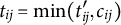 $t_{ij} = \min (t^{\prime }_{ij},c_{ij}) $
is the minimum of the processing time (first hitting time plus non-decision time)
$t_{ij} = \min (t^{\prime }_{ij},c_{ij}) $
is the minimum of the processing time (first hitting time plus non-decision time) $t^{\prime }_{ij}$
and the censoring time
$t^{\prime }_{ij}$
and the censoring time $c_{ij}$
. The distribution of the observed responses and response times can be derived from standard findings for race models.
$c_{ij}$
. The distribution of the observed responses and response times can be derived from standard findings for race models.
In the diffIRT-R model, a specific response is given in case the diffusion process wins by hitting the corresponding boundary before the censoring time or in the case the censoring process wins and the given response is selected by a random guess. Random guesses are generated by a Bernoulli experiment with fixed guessing probability $\pi $
. The defective density function of the response
$\pi $
. The defective density function of the response $x_{ij}$
(1: Correct, 0: Incorrect) and the observed response time
$x_{ij}$
(1: Correct, 0: Incorrect) and the observed response time $t_{ij}$
of a test taker i with fixed latent traits
$t_{ij}$
of a test taker i with fixed latent traits $(\theta _i,\omega _i,\tau _i)$
in item j is
$(\theta _i,\omega _i,\tau _i)$
in item j is
 $$ \begin{align} \text{f} \big(x_{ij},t_{ij}; & \, v_j(\theta_i),a_j(\omega_i),d_j, \mu_j(\tau_i), \sigma_j, \pi \big) \notag \\ & = \text{f}_{\text{D}} \big(x_{ij},t_{ij}; v_j(\theta_i),a_j(\omega_i),d_j \big) \cdot \text{S}_{\text{C}}\big( t_{ij}; \mu_j(\tau_i), \sigma_j \big) \\ & \ \ \ + \text{f}_{\text{C}}\big( t_{ij}; \mu_j(\tau_i), \sigma_j \big) \cdot \text{S}_{\text{D}}\big(t_{ij}; v_j(\theta_i),a_j(\omega_i),d_j \big) \cdot (\pi)^{x_{ij}} \cdot (1-\pi)^{1-x_{ij}}. \notag \end{align} $$
Functions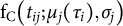 $\text {f}_{\text {C}}\big ( t_{ij}; \mu _j(\tau _i), \sigma _j \big )$
and
$\text {f}_{\text {C}}\big ( t_{ij}; \mu _j(\tau _i), \sigma _j \big )$
and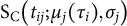 $\text {S}_{\text {C}}\big ( t_{ij}; \mu _j(\tau _i), \sigma _j \big )$
are the density function and the survival function of the log-normal distribution (Crow & Shimizu, Reference Crow and Shimizu1988) with scale parameter
$\text {S}_{\text {C}}\big ( t_{ij}; \mu _j(\tau _i), \sigma _j \big )$
are the density function and the survival function of the log-normal distribution (Crow & Shimizu, Reference Crow and Shimizu1988) with scale parameter $\mu _j(\tau _i)$
and shape parameter
$\mu _j(\tau _i)$
and shape parameter $\sigma _j$
, respectively. Function
$\sigma _j$
, respectively. Function $\text {f}_{\text {D}}\big (x_{ij},t_{ij}; v_j(\theta _i),a_j(\omega _i),d_j \big )$
is the defective density function of the response and the response time implied by the diffusion process with drift rate
$\text {f}_{\text {D}}\big (x_{ij},t_{ij}; v_j(\theta _i),a_j(\omega _i),d_j \big )$
is the defective density function of the response and the response time implied by the diffusion process with drift rate $v_j(\theta _i)$
, boundary separation
$v_j(\theta _i)$
, boundary separation $a_j(\omega _i),$
and shift parameter
$a_j(\omega _i),$
and shift parameter $d_j$
(Tuerlinckx & De Boeck, Reference Tuerlinckx and De Boeck2005, Equation 3). Function
$d_j$
(Tuerlinckx & De Boeck, Reference Tuerlinckx and De Boeck2005, Equation 3). Function $\text {S}_{\text {D}}\big (t_{ij}; v_j(\theta _i),a_j(\omega _i),d_j\big )$
is the survival function of the diffusion process. In Equation (4), the first term accounts for the case that the censoring process loses and the response is determined by the diffusion process, while the second term accounts for the case that the diffusion process loses and the response is determined by a random guess (see Supplement 1 for more details).
$\text {S}_{\text {D}}\big (t_{ij}; v_j(\theta _i),a_j(\omega _i),d_j\big )$
is the survival function of the diffusion process. In Equation (4), the first term accounts for the case that the censoring process loses and the response is determined by the diffusion process, while the second term accounts for the case that the diffusion process loses and the response is determined by a random guess (see Supplement 1 for more details).
In the diffIRT-I model, a specific response is given in case the diffusion process wins by hitting the corresponding boundary before the censoring time or the censoring process wins and the given response is determined by the sign rule. The defective density function of the response $x_{ij}$
(1: Correct, 0: Incorrect) and the observed response time
$x_{ij}$
(1: Correct, 0: Incorrect) and the observed response time $t_{ij}$
of a test taker i with fixed latent traits
$t_{ij}$
of a test taker i with fixed latent traits $(\theta _i,\omega _i,\tau _i)$
in item j is
$(\theta _i,\omega _i,\tau _i)$
in item j is
 $$ \begin{align} \text{f} \big(x_{ij},t_{ij}; & \, v_j(\theta_i),a_j(\omega_i),d_j, \mu_j(\tau_i), \sigma_j \big) \notag \\ & = \text{f}_{\text{D}} \big(x_{ij},t_{ij}; v_j(\theta_i),a_j(\omega_i),d_j \big) \cdot \text{S}_{\text{C}}\big( t_{ij}; \mu_j(\tau_i), \sigma_j \big) \\ & \ \ \ + \text{f}_{\text{C}}\big( t_{ij}; \mu_j(\tau_i), \sigma_j \big) \cdot \text{S}^{*}_{\text{D}}\big(x_{ij},t_{ij}; v_j(\theta_i),a_j(\omega_i),d_j \big). \notag \end{align} $$
As before, function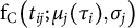 $\text {f}_{\text {C}}\big ( t_{ij}; \mu _j(\tau _i), \sigma _j \big )$
is the density function of the log-normal distribution, function
$\text {f}_{\text {C}}\big ( t_{ij}; \mu _j(\tau _i), \sigma _j \big )$
is the density function of the log-normal distribution, function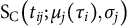 $\text {S}_{\text {C}}\big ( t_{ij}; \mu _j(\tau _i), \sigma _j \big )$
is the survival function, and function
$\text {S}_{\text {C}}\big ( t_{ij}; \mu _j(\tau _i), \sigma _j \big )$
is the survival function, and function $\text {f}_{\text {D}}\big (x_{ij},t_{ij}; v_j(\theta _i),a_j(\omega _i),d_j \big )$
is the defective density function of the response and the response time implied by the diffusion process. Function
$\text {f}_{\text {D}}\big (x_{ij},t_{ij}; v_j(\theta _i),a_j(\omega _i),d_j \big )$
is the defective density function of the response and the response time implied by the diffusion process. Function $\text {S}^{*}_{\text {D}}\big ( x_{ij},t_{ij}; v_j(\theta _i),a_j(\omega _i),d_j \big )$
denotes the probability that the hitting time of the diffusion process is longer than
$\text {S}^{*}_{\text {D}}\big ( x_{ij},t_{ij}; v_j(\theta _i),a_j(\omega _i),d_j \big )$
denotes the probability that the hitting time of the diffusion process is longer than $t_{ij}$
and the value of the accumulator is positive (
$t_{ij}$
and the value of the accumulator is positive ( $X(t_{ij})>0$
) when
$X(t_{ij})>0$
) when $x_{ij}=1$
or negative (
$x_{ij}=1$
or negative ( $X(t_{ij})<0$
) when
$X(t_{ij})<0$
) when $x_{ij}=0$
at
$x_{ij}=0$
at $t_{ij}$
. This probability follows from the distribution of the accumulator in non-terminated processes at the censoring time (Ratcliff, Reference Ratcliff1980, Equation 12/13). The distribution has to be integrated from
$t_{ij}$
. This probability follows from the distribution of the accumulator in non-terminated processes at the censoring time (Ratcliff, Reference Ratcliff1980, Equation 12/13). The distribution has to be integrated from $0$
to
$0$
to $a/2$
in case the response is correct and from
$a/2$
in case the response is correct and from $0$
to
$0$
to $-a/2$
in case the response is incorrect. In Equation (5), the first term accounts for the case that the censoring process loses and the response is determined by the diffusion process, while the second term accounts for the case that the diffusion process loses and the response is determined by the sign of the accumulator (see Supplement 1 for more details).
$-a/2$
in case the response is incorrect. In Equation (5), the first term accounts for the case that the censoring process loses and the response is determined by the diffusion process, while the second term accounts for the case that the diffusion process loses and the response is determined by the sign of the accumulator (see Supplement 1 for more details).
The functions in Equation (4) or Equation (5) are the defective density functions of the response and the response time of test takers with fixed latent traits $(\theta _i,\omega _i,\tau _i)$
on a single item. They specify the distribution of the response and response time conditional on the latent traits. The joint distribution of the responses and response times of a test taker with fixed trait levels on all items of a test follows from the factorization theorem if one makes the conditional independence assumption. The marginal distribution of the responses and response times is the unconditional distribution when latent traits are also sampled randomly. It is obtained by integrating the conditional distribution over the distribution of the latent traits in the population of the potential test takers. This requires an assumption about the distribution of the latent traits. Here, we assume that the latent traits are multivariate normally distributed, with expected values of zero, variances of one, and correlation matrix
$(\theta _i,\omega _i,\tau _i)$
on a single item. They specify the distribution of the response and response time conditional on the latent traits. The joint distribution of the responses and response times of a test taker with fixed trait levels on all items of a test follows from the factorization theorem if one makes the conditional independence assumption. The marginal distribution of the responses and response times is the unconditional distribution when latent traits are also sampled randomly. It is obtained by integrating the conditional distribution over the distribution of the latent traits in the population of the potential test takers. This requires an assumption about the distribution of the latent traits. Here, we assume that the latent traits are multivariate normally distributed, with expected values of zero, variances of one, and correlation matrix $\boldsymbol {\Sigma }$
. Assumptions about the expectation and variance are necessary in order to identify the scale of the latent traits.
$\boldsymbol {\Sigma }$
. Assumptions about the expectation and variance are necessary in order to identify the scale of the latent traits.
2 Simulation study
We conducted three simulation studies. In the first study, we investigated parameter recovery with marginal maximum likelihood (MML) estimation. In the second study, we investigated whether information criteria accurately identify the data-generating model among several alternatives. In the third study, we investigated the performance of the proposed models as measurement models of the latent traits and their capability to detect premature responses.
2.1 Simulation study I: Parameter recovery
In the first study, we generated data according to the extended diffIRT models, estimated the values of the models’ parameters with MML estimation, and compared the estimates to the true values of the parameters. We considered $2 \times 2$
simulation conditions defined by the model (diffIRT-R/diffIRT-I) and the sample size (
$2 \times 2$
simulation conditions defined by the model (diffIRT-R/diffIRT-I) and the sample size ( $N=500$
/
$N=500$
/ $N=1,000$
). The number of items was set to
$N=1,000$
). The number of items was set to $J=24$
. For each simulation condition, we analyzed 100 simulation samples.
$J=24$
. For each simulation condition, we analyzed 100 simulation samples.
Data were generated as follows. We first simulated values for the latent traits of fictitious test takers by random draws from a standardized multivariate normal distribution. For all fictitious test takers and items, we determined the parameters of the diffusion model ( $v_j(\theta _i)$
,
$v_j(\theta _i)$
, $a_j(\omega _i)$
) and the log-normal distribution (
$a_j(\omega _i)$
) and the log-normal distribution ( $\mu _j(\tau _i)$
) according to Equations (2) and (3). We then drew censoring times from a log-normal distribution with parameters
$\mu _j(\tau _i)$
) according to Equations (2) and (3). We then drew censoring times from a log-normal distribution with parameters $\mu _j( \tau _i )$
and
$\mu _j( \tau _i )$
and $\sigma _j$
and simulated the diffusion process with parameters
$\sigma _j$
and simulated the diffusion process with parameters $v_j(\theta _i)$
,
$v_j(\theta _i)$
, $a_j(\omega _i),$
and
$a_j(\omega _i),$
and $d_j$
using the Sim.DiffProc package (Guidoum & Boukhetala, Reference Guidoum and Boukhetala2020) from the statistical computing environment R (R Core Team, 2021). The responses and the response times were determined as illustrated in Figure 1. In the diffIRT-R model, the premature responses were random guesses generated according to a Bernoulli experiment with parameter
$d_j$
using the Sim.DiffProc package (Guidoum & Boukhetala, Reference Guidoum and Boukhetala2020) from the statistical computing environment R (R Core Team, 2021). The responses and the response times were determined as illustrated in Figure 1. In the diffIRT-R model, the premature responses were random guesses generated according to a Bernoulli experiment with parameter $\pi =0.2$
. In the diffIRT-I model, the premature responses were generated according to the sign rule.
$\pi =0.2$
. In the diffIRT-I model, the premature responses were generated according to the sign rule.
For data generation, we used the following model parameters. The correlations of the traits were set to $\rho _{\theta \omega }=0.40$
,
$\rho _{\theta \omega }=0.40$
, $\rho _{\theta \tau }=0.20,$
and
$\rho _{\theta \tau }=0.20,$
and $\rho _{\omega \tau }=0.30$
. We used positive values as we assumed that test takers with higher capability are also more engaged. The item parameters of the diffusion model were set to the values
$\rho _{\omega \tau }=0.30$
. We used positive values as we assumed that test takers with higher capability are also more engaged. The item parameters of the diffusion model were set to the values $a_{0j} \in \{ 2.5,3.0,3.5 \}$
,
$a_{0j} \in \{ 2.5,3.0,3.5 \}$
, $a_{1j} \in \{ 0.8,1.2 \}$
,
$a_{1j} \in \{ 0.8,1.2 \}$
, $v_{0j} \in \{ -1.0,-0.5,0.5,1.0 \}$
,
$v_{0j} \in \{ -1.0,-0.5,0.5,1.0 \}$
, $v_{1j} \in \{ 0.8,1.2 \},$
and
$v_{1j} \in \{ 0.8,1.2 \},$
and $d_{j} \in \{ 0.25 \}$
. The item parameters of the log-normal model were set to the values
$d_{j} \in \{ 0.25 \}$
. The item parameters of the log-normal model were set to the values $c_{0j} \in \{ 0.9,1.1 \}$
,
$c_{0j} \in \{ 0.9,1.1 \}$
, $c_{1j} \in \{ 0.3 \},$
and
$c_{1j} \in \{ 0.3 \},$
and $\sigma _{j} \in \{ 0.4 \}$
. The guessing probability of the diffIRT-R model was set to
$\sigma _{j} \in \{ 0.4 \}$
. The guessing probability of the diffIRT-R model was set to $\pi =0.2$
. When generating the data, we intended to mimic the data from a test on mental rotation (Gaviria, Reference Gaviria2005). We, however, extended the range of
$\pi =0.2$
. When generating the data, we intended to mimic the data from a test on mental rotation (Gaviria, Reference Gaviria2005). We, however, extended the range of $v_{0j}$
in order have more variation in the item difficulties than the mental rotation items had. We also took care to induce a rather low amount of disengaged responding as even in low stakes tests, most test takers are motivated to do well (e.g., Michaelides et al., Reference Michaelides, Ivanova and Nicolaou2020; Wise, Reference Wise2017). A detailed list of the parameters values in all items is given in Supplementary Table S2.1.
$v_{0j}$
in order have more variation in the item difficulties than the mental rotation items had. We also took care to induce a rather low amount of disengaged responding as even in low stakes tests, most test takers are motivated to do well (e.g., Michaelides et al., Reference Michaelides, Ivanova and Nicolaou2020; Wise, Reference Wise2017). A detailed list of the parameters values in all items is given in Supplementary Table S2.1.
For each data set, the parameters of the data-generating model were estimated using MML estimation. In MML estimation, one determines those values of the model parameters that maximize the marginal likelihood function (Berger et al., Reference Berger, Liseo and Wolpert1999, see Integrated Likelihood). The marginal likelihood function was implemented in the Julia programming language (Bezanson et al., Reference Bezanson, Edelman, Karpinski and Shah2017). The density function of the diffusion model was evaluated with the DiffModels.jl package (Drugowitsch, Reference Drugowitsch2017). The function $\text {S}^{*}_{\text {D}}\big ( x_{ij},t_{ij}; v_j(\theta _i),a_j(\omega _i),d_j \big )$
was approximated by limiting the infinite sum to 30 terms. This approximation was sufficient for the present application. Integrals over the latent traits were approximated with the Mislevy quadrature using 20 nodes in case of the diffIRT-R model and 15 nodes in case of the diffIRT-I model (Kim et al., Reference Kim, Bao, Horan, Kim, Cohen, Ark, Bolt, Wang, Douglas and Chow2015). We reduced the number of nodes in the diffIRT-I model in order to save computation time. The marginal likelihood function was maximized within the statistical computing environment R. We used the package optim and the BFGS algorithm (Nocedal & Wright, Reference Nocedal and Wright2006). In addition to point estimates, we also determined Wald-type confidence intervals for a confidence level of
$\text {S}^{*}_{\text {D}}\big ( x_{ij},t_{ij}; v_j(\theta _i),a_j(\omega _i),d_j \big )$
was approximated by limiting the infinite sum to 30 terms. This approximation was sufficient for the present application. Integrals over the latent traits were approximated with the Mislevy quadrature using 20 nodes in case of the diffIRT-R model and 15 nodes in case of the diffIRT-I model (Kim et al., Reference Kim, Bao, Horan, Kim, Cohen, Ark, Bolt, Wang, Douglas and Chow2015). We reduced the number of nodes in the diffIRT-I model in order to save computation time. The marginal likelihood function was maximized within the statistical computing environment R. We used the package optim and the BFGS algorithm (Nocedal & Wright, Reference Nocedal and Wright2006). In addition to point estimates, we also determined Wald-type confidence intervals for a confidence level of $c=0.95$
(
$c=0.95$
( $\alpha =0.05$
) using the observed information matrix. The observed information matrix was approximated by the variance–covariance matrix of the score values.
$\alpha =0.05$
) using the observed information matrix. The observed information matrix was approximated by the variance–covariance matrix of the score values.
The results of the simulation study are summarized in Table 1 for the diffIRT-R model and in Table 2 for the diffIRT-I model. In both tables, we report the true value (TV), the average estimate (M), the standard of error of estimation of the parameters (SE), and the coverage frequency (CI) of confidence intervals. For ease of presentation, the results concerning the parameters have been averaged over items with the same value.
True value (TV), average estimate (M), standard error of estimation (SE), and coverage frequency (CI) of confidence intervals of the parameter estimates for different samples sizes N in the diffIRT-R model with random guessing

Note: Results are based on 100 simulation samples. Results for parameters have been averaged over the items of with the same parameter values. Confidence intervals were determined for a confidence level of $c=0.95 (\alpha =0.05)$
. Standard error of estimation refers to the parameter estimates.
$c=0.95 (\alpha =0.05)$
. Standard error of estimation refers to the parameter estimates.
True value (TV), average estimate (M), standard error of estimation (SE), and coverage frequency (CI) of confidence intervals of the parameter estimates for different samples sizes N in the diffIRT-I model where premature responses are generated by the sign rule

Note: Results are based on 100 simulation samples. Results for parameters have been averaged over the items of with the same parameter values. Confidence intervals were determined for a confidence level of $c=0.95 (\alpha =0.05)$
. Standard error of estimation refers to the parameter estimates.
$c=0.95 (\alpha =0.05)$
. Standard error of estimation refers to the parameter estimates.
In the diffIRT-R model, the MML estimator is virtually unbiased in most parameters. There is a slight bias in parameter $a_0$
for both sample sizes and in parameter
$a_0$
for both sample sizes and in parameter $\sigma $
for samples of
$\sigma $
for samples of $N=500$
subjects. The bias, however, is not large and should not have any significance in practice. The coverage frequencies of the confidence intervals exceed the intended level of
$N=500$
subjects. The bias, however, is not large and should not have any significance in practice. The coverage frequencies of the confidence intervals exceed the intended level of $c=0.95$
. In samples of
$c=0.95$
. In samples of $N=1,000$
, the coverage frequencies are closer to the intended level of
$N=1,000$
, the coverage frequencies are closer to the intended level of $c=0.95$
, but still slightly too high.
$c=0.95$
, but still slightly too high.
In the diffIRT-I model, the MML estimator is virtually unbiased in all parameters except parameter $\sigma $
. Results concerning the coverage frequencies of the confidence intervals depend on the sample size. In samples of
$\sigma $
. Results concerning the coverage frequencies of the confidence intervals depend on the sample size. In samples of $N=500$
, the coverage frequencies are slightly too high in the parameters of the diffusion model, but slightly too low in the parameters of the log-normal model and the coefficients of correlation. In samples of
$N=500$
, the coverage frequencies are slightly too high in the parameters of the diffusion model, but slightly too low in the parameters of the log-normal model and the coefficients of correlation. In samples of $N=1,000$
, the coverage frequencies are close to the intended level of
$N=1,000$
, the coverage frequencies are close to the intended level of $c=0.95$
.
$c=0.95$
.
2.2 Simulation study II: Model selection
In the second simulation study, we addressed the question whether the diffIRT models can be distinguished empirically. For the study, we used the data sets with $N=1,000$
subjects that were generated in the first simulation study. We did not consider the data sets with
$N=1,000$
subjects that were generated in the first simulation study. We did not consider the data sets with $N=500$
subjects due to the high time demand of the data analysis. Each data set was analyzed with the diffIRT, diffIRT-I, and diffIRT-R models. We estimated the item parameters of each model with MML estimation as in the first simulation study. We then determined the Akaike information criterion (AIC) of Akaike, (Reference Akaike, Kotz and Johnson1992) and the Bayes information criterion (BIC) of Schwarz, (Reference Schwarz1978) for the three models. The model with the lowest AIC or BIC value was selected as the one that was presumed to have generated the data (Burnham & Anderson, Reference Burnham and Anderson2013). The relative frequencies by which each model was selected are reported in Table 3 separately for the two information criteria conditional on the true data-generating model.
$N=500$
subjects due to the high time demand of the data analysis. Each data set was analyzed with the diffIRT, diffIRT-I, and diffIRT-R models. We estimated the item parameters of each model with MML estimation as in the first simulation study. We then determined the Akaike information criterion (AIC) of Akaike, (Reference Akaike, Kotz and Johnson1992) and the Bayes information criterion (BIC) of Schwarz, (Reference Schwarz1978) for the three models. The model with the lowest AIC or BIC value was selected as the one that was presumed to have generated the data (Burnham & Anderson, Reference Burnham and Anderson2013). The relative frequencies by which each model was selected are reported in Table 3 separately for the two information criteria conditional on the true data-generating model.
Relative frequencies by which a model was selected as the alleged data-generating model for the information criteria AIC and BIC conditional on the true data-generating model

Note: Results are based on 100 simulation samples. diffIRT: Diffusion model without censoring; diffIRT-R: Diffusion model with censoring and random guessing; diffIRT-I: Diffusion model with censoring and premature responding based on the sign rule.
In all simulation samples, the data-generating model is identified correctly. This suggests that the models can be distinguished empirically. The diffIRT model, for example, predicts generally longer response times than the diffIRT-I and diffIRT-R models. The diffIRT-I models and the diffIRT-R in turn differ in the accuracy of premature responses.
2.3 Simulation study III: Trait recovery
In the third simulation study, we investigated whether the latent traits can be estimated reliably with maximum likelihood estimation, how trait recovery depends on the censoring rate and whether premature responses can be detected.
True value (TV), average estimate (M), standard error of estimation (SE), and coverage frequency (CI) of confidence intervals of the trait estimates for different item number J and the two extended diffIRT models

Note: Results for a trait have been averaged over the other traits. Results are based on 450 data patterns. Confidence intervals were determined for a level of confidence of $c=0.95 (\alpha =0.05)$
. diffIRT-R: Diffusion model with censoring and random guessing; diffIRT-I: Diffusion model with censoring and premature responses based on the sign rule.
$c=0.95 (\alpha =0.05)$
. diffIRT-R: Diffusion model with censoring and random guessing; diffIRT-I: Diffusion model with censoring and premature responses based on the sign rule.
The simulation study was implemented as follows. By fully crossing nine trait levels $\{-2.0,-1.5,\ldots ,1.5,2.0 \}$
, we defined
$\{-2.0,-1.5,\ldots ,1.5,2.0 \}$
, we defined $729$
fictitious test takers who were characterized by a unique combination of capability, response caution, and willingness to invest time. We used fixed trait levels in order to study whether the maximum likelihood estimator is conditionally unbiased. For each test taker, we generated
$729$
fictitious test takers who were characterized by a unique combination of capability, response caution, and willingness to invest time. We used fixed trait levels in order to study whether the maximum likelihood estimator is conditionally unbiased. For each test taker, we generated $50$
responses and response time patterns with the diffIRT-I and diffIRT-R models. We considered a test with 24 items and a test with 48 items. For the test with 24 items, we used the same item parameters as in the first simulation study on parameter recovery. For the test with 48 items, we used each item twice. Data generation resulted in
$50$
responses and response time patterns with the diffIRT-I and diffIRT-R models. We considered a test with 24 items and a test with 48 items. For the test with 24 items, we used the same item parameters as in the first simulation study on parameter recovery. For the test with 48 items, we used each item twice. Data generation resulted in $729 \times 50$
response and response time pattern for each condition defined by the data-generating model and the length of the test.
$729 \times 50$
response and response time pattern for each condition defined by the data-generating model and the length of the test.
We estimate the latent traits of all fictitious test takers with maximum likelihood estimation. The values of the item parameters were set to the true values. The true values of the item parameters were used to prevent confounding of item parameter and trait estimation. In addition to point estimates of the trait values, we determined Wald-type confidence intervals for a confidence level of $c=0.95$
(
$c=0.95$
( $\alpha =0.05$
). The standard errors of estimation were determined by inverting the negative Hessian matrix. The Hessian matrix was approximated using numerical methods. We evaluated the maximum likelihood estimator with respect to the average estimate, the standard error of estimation, and the coverage frequency of the confidence intervals. The results are given in Table 4. Results for one trait have been aggregated over the other traits.
$\alpha =0.05$
). The standard errors of estimation were determined by inverting the negative Hessian matrix. The Hessian matrix was approximated using numerical methods. We evaluated the maximum likelihood estimator with respect to the average estimate, the standard error of estimation, and the coverage frequency of the confidence intervals. The results are given in Table 4. Results for one trait have been aggregated over the other traits.
Rate of false alarms (FA), detection rate (DR), and correlation (R) between the true number of premature responses and the predicted number when responses are flagged as premature with the extended diffIRT models and the estimated trait levels depending on the item number J

Note: Results are based on 36,450 data patterns and are averaged over the items. diffIRT-R: Diffusion model with censoring and random guessing; diffIRT-I: Diffusion model with censoring and premature responding based on the sign rule.
In the condition with $24$
items, the estimator of capability has a small bias and large standard errors of estimation. The standard errors would correspond to reliability coefficients between
$24$
items, the estimator of capability has a small bias and large standard errors of estimation. The standard errors would correspond to reliability coefficients between $0.22$
and
$0.22$
and $0.95$
in case the squared standard errors were interpreted as the error variance. The large standard errors are partly due to a small proportion of extreme estimates. Coverage frequencies of the confidence intervals are close to the intended level of
$0.95$
in case the squared standard errors were interpreted as the error variance. The large standard errors are partly due to a small proportion of extreme estimates. Coverage frequencies of the confidence intervals are close to the intended level of $0.95$
. In the condition with 48 items, the estimator is virtually unbiased and the standard errors of estimation are considerably smaller. The implied reliability coefficients are in the range from 0.77 to 0.98. The willingness to invest time does not impact the estimation of capability much (see Supplementary Figures S3.1 and S3.4). Though, the standard errors tend to be slightly larger when the willingness to invest time is low, especially for the diffIRT-R model. Presumably, this is because censored responses provide little information about a test taker’s capability when they are generated through random guessing.
$0.95$
. In the condition with 48 items, the estimator is virtually unbiased and the standard errors of estimation are considerably smaller. The implied reliability coefficients are in the range from 0.77 to 0.98. The willingness to invest time does not impact the estimation of capability much (see Supplementary Figures S3.1 and S3.4). Though, the standard errors tend to be slightly larger when the willingness to invest time is low, especially for the diffIRT-R model. Presumably, this is because censored responses provide little information about a test taker’s capability when they are generated through random guessing.
The estimator of response caution is biased in all conditions. The bias is smaller in the condition with $48$
items than in the condition with
$48$
items than in the condition with $24$
items. Standard errors are high. The corresponding reliability coefficients range from 0.02 to 0.62 in the test with 24 items and from 0.15 to 0.98 in the test with 48 items. Standard errors are higher and reliabilities are lower for high levels of response caution. Low levels of response caution, however, can be estimated well. Supplementary Figures S3.2 and S3.5 suggest that the reliability depends on the willingness to invest time. The standard error of estimation is highest when a high level of response caution is combined with a low willingness to invest time. This combination is especially problematic for the diffIRT-R model. In that case, almost all of the responses are random guesses that have no direct connection to the diffusion process.
$24$
items. Standard errors are high. The corresponding reliability coefficients range from 0.02 to 0.62 in the test with 24 items and from 0.15 to 0.98 in the test with 48 items. Standard errors are higher and reliabilities are lower for high levels of response caution. Low levels of response caution, however, can be estimated well. Supplementary Figures S3.2 and S3.5 suggest that the reliability depends on the willingness to invest time. The standard error of estimation is highest when a high level of response caution is combined with a low willingness to invest time. This combination is especially problematic for the diffIRT-R model. In that case, almost all of the responses are random guesses that have no direct connection to the diffusion process.
Results are similar for the willingness to invest time. The estimator has a large bias, especially in the diffIRT-R model and the condition with 24 items. Standard errors are high. Corresponding reliability coefficients range from 0.19 to 0.46 in the test with 24 items and from 0.21 to 0.59 in the test with 48 items. The coverage frequencies of the confidence intervals are below the intended level of 0.95. The reliability of the estimates depends on the level of response caution. Supplementary Figures S3.3 and S3.6 suggest that high levels of the willingness to invest time cannot be estimated well when the response caution is low. In this case, the diffusion process wins in most cases.
In an additional analysis, we compared the trait estimates from the extended diffIRT models to those from a misspecified diffIRT model. For this purpose, we determined the diffIRT model that best approximated the extended versions in the Kullback–Leibler sense (White, Reference White1982). We then used this misspecified diffIRT model in order to estimate the capability and the response caution with the generated data. The bias of the trait estimates is visualized in Figure 2 as a function of the rate of premature responding. We also report the bias of the trait estimates when the data-generating model (diffIRT-R/diffIRT-I) is used for trait estimation.
Bias of the estimates of capability $\theta $
and response caution
$\theta $
and response caution $\omega $
when the data-generating model and when the standard diffusion model is used for estimation as a function of the rate of premature responses (censoring rate).
$\omega $
when the data-generating model and when the standard diffusion model is used for estimation as a function of the rate of premature responses (censoring rate).

When data are generated according to the diffIRT-I model, the estimates of capability are virtually unbiased irrespective of whether the diffIRT-I or the misspecified diffIRT model is used as the measurement model. This is even the case when almost all responses are generated prematurely. The estimates of the response caution, however, are affected by the misspecification of the measurement model. When data are generated according to the diffIRT-R model, the estimates of capability are biased when the misspecified diffIRT model is used as the measurement model. The estimates provided by the diffIRT-R model remain unbiased, even when almost all responses are premature. The estimates of response caution, however, have a bias in both models when the rate of premature responses exceeds 50%. The bias, however, decreases in the diffIRT-R model when more items are used for trait estimation.
Finally, we investigated whether premature responses can be detected. We used the data-generating model (diffIRT-I/diffIRT-R) and the trait estimates in order to determine the posterior probability that a response was premature. Responses were flagged as premature when the posterior probability exceeded 0.5. Table 5 contains the detection rate, the rate of false alarms, and the correlation between the true number of premature responses and the predicted number of premature responses. A plot of the true number of premature responses against the expected number is given in the Supplementary Material (see Supplement 2 and Supplementary Figure S3.9).
The models are relatively successful in detecting premature responses. The number of premature responses can be predicted well, especially with the diffIRT-R model. The models are also capable to detect more than half of the premature responses. The rate of false alarms is relatively low.
3 Empirical application
We analyzed two data sets with the extended diffIRT models. The data sets consisted of the responses and response times of test takers on different cognitive tests. The tests varied in their cognitive demands and response formats. We selected the data sets to explore the conditions under which the model can used. This question is particularly relevant for process models that rely on strong assumptions about the response process and may not be suitable in all contexts (Krämer et al., Reference Krämer, Ranger, Koch, Spinath and Schmitz2025). We used the following data sets.
3.1 SPT
The SPT data set comprised responses and response times of 773 university students on 16 items of a test on visuo-spatial perspective taking (Kessler & Thomson, Reference Kessler and Thomson2010). Each item depicted a target person seated at a round table from a bird’s-eye perspective. The person’s position at the table was rotated between 120 $^{\circ }$
, 160
$^{\circ }$
, 160 $^{\circ }$
, 200
$^{\circ }$
, 200 $^{\circ }$
, or 240
$^{\circ }$
, or 240 $^{\circ }$
relative to the test taker’s point of view. Test takers were asked to judge whether a specific object on the table was closer to the person’s left or right arm. Data were collected by Wolgast et al., (Reference Wolgast, Schmidt and Ranger2020) in a low-stakes setting and are available on OSF (https://osf.io/nmxq7/). Before analyzing the data, we removed data from test takers with irregular long response times. Response times were defined as irregular long when they exceeding the median time by
$^{\circ }$
relative to the test taker’s point of view. Test takers were asked to judge whether a specific object on the table was closer to the person’s left or right arm. Data were collected by Wolgast et al., (Reference Wolgast, Schmidt and Ranger2020) in a low-stakes setting and are available on OSF (https://osf.io/nmxq7/). Before analyzing the data, we removed data from test takers with irregular long response times. Response times were defined as irregular long when they exceeding the median time by $2.5$
times the inter quartile range. Such long response times likely reflect interruptions of the solution process that fall outside the scope of the model. Data cleaning reduced the data set to
$2.5$
times the inter quartile range. Such long response times likely reflect interruptions of the solution process that fall outside the scope of the model. Data cleaning reduced the data set to $744$
subjects. In the cleaned data set, the solution frequencies ranged from
$744$
subjects. In the cleaned data set, the solution frequencies ranged from $0.92$
to
$0.92$
to $0.94$
and the average response times varied between
$0.94$
and the average response times varied between $1.64$
to
$1.64$
to $2.02$
seconds. We selected the data set as we considered it well-suited for an analysis with the diffusion model: The response process involves basic mental operations and a binary decision. The applicability of the diffusion model to data from mental rotation tests has been demonstrated in prior research (Molenaar et al., Reference Molenaar, Tuerlinckx and van der Maas2015; van der Maas et al., Reference van der Maas, Molenaar, Maris, Kievit and Borsboom2011).
$2.02$
seconds. We selected the data set as we considered it well-suited for an analysis with the diffusion model: The response process involves basic mental operations and a binary decision. The applicability of the diffusion model to data from mental rotation tests has been demonstrated in prior research (Molenaar et al., Reference Molenaar, Tuerlinckx and van der Maas2015; van der Maas et al., Reference van der Maas, Molenaar, Maris, Kievit and Borsboom2011).
3.2 PERC
The PERC data set comprised the responses and response times of 2,978 high school students on 15 Raven matrix tasks measuring abstract reasoning (Raven et al., Reference Raven, Raven and Court1998). Each item consisted of a matrix of figures which was generated by certain rules. One element of the matrix was missing. Test takers had to choose from a set of figures the one that complemented the matrix consistently. The items were grouped into five blocks. The first block consisted of easy tasks. Its purpose was to create an experience of success. The second block consisted of medium difficult tasks. After the tasks, the test takers received feedback and could access tips on how to improve their performance. Usage of the tips is interpreted as a measure of effort. The third block consisted of very difficult tasks. The time on task in the third block is interpreted as a measure of persistence. The final block consisted of easy tasks that were matched in difficulty to the tasks in the first set. Differences in performance between the first block and the last block are interpreted as a measure of resilience. Data were collected by Porter et al. (Reference Porter, Catalán Molina, Blackwell, Roberts, Quirk, Lee Duckworth and Trzesniewski2020) in a low-stakes setting and are publicly available on OSF (https://osf.io/8xcjp/). For the analysis, we only considered the 1,680 cases with complete data that had previously been analyzed by Domingue et al. (Reference Domingue, Kanopka, Stenhaug, Sulik, Beverly, Brinkhuis, Circi, Faul, Liao, McCandliss, Obradovic, Piech, Porter, Soland, Weeks, Wise and Yeatman2022). We removed test takers with unusually long response times as in the SPT data set. This reduced the data set to 1,560 subjects. In the reduced data set, the solution frequencies ranged from 0.10 to 0.97 and the average response times varied between 8.48 and 57.08 seconds. We included the data set as we wanted to assess whether the model can be used when tests involve more complex mental operations. Furthermore, we expected censoring in the difficult items.
We fitted several models to both data sets. We fitted a standard diffIRT model with ( $d_j \neq 0$
) and without (
$d_j \neq 0$
) and without ( $d_j=0$
) a non-decision time. We fitted both versions of the extended diffIRT model, also either with (
$d_j=0$
) a non-decision time. We fitted both versions of the extended diffIRT model, also either with ( $d_j \neq 0$
) and without (
$d_j \neq 0$
) and without ( $d_j=0$
) a non-decision time. In the diffIRT-R model with random guessing, the guessing probabilities across the items were constrained to be equal. This restriction simplifies parameter estimation and is justified in case guessing is indeed random. For the sake of comparison, we also fitted the hierarchical model proposed by van der Linden (Reference van der Linden2007) to the data. The hierarchical model is one of the most popular models for responses and response times on tests and was included as a benchmark. It combines an item response theory (IRT) model for the responses and a log-normal factor model for the response times. We considered several versions of the hierarchical model, using either a two-parameter logistic (2-PL) or a three-parameter logistic (3-PL) model for the responses, and a log-normal factor model with or without a shift parameter for the response times. All models were fitted with MML estimation. We compared the relative fit of the models with the AIC index and the BIC index. Results concerning relative model fit are given in Table 6 where we report the marginal log-likelihood (LL), the number of model parameters (NP), the AIC index, and the BIC index, as well as the difference between the information criterion for each model and that for the best fitting model (
$d_j=0$
) a non-decision time. In the diffIRT-R model with random guessing, the guessing probabilities across the items were constrained to be equal. This restriction simplifies parameter estimation and is justified in case guessing is indeed random. For the sake of comparison, we also fitted the hierarchical model proposed by van der Linden (Reference van der Linden2007) to the data. The hierarchical model is one of the most popular models for responses and response times on tests and was included as a benchmark. It combines an item response theory (IRT) model for the responses and a log-normal factor model for the response times. We considered several versions of the hierarchical model, using either a two-parameter logistic (2-PL) or a three-parameter logistic (3-PL) model for the responses, and a log-normal factor model with or without a shift parameter for the response times. All models were fitted with MML estimation. We compared the relative fit of the models with the AIC index and the BIC index. Results concerning relative model fit are given in Table 6 where we report the marginal log-likelihood (LL), the number of model parameters (NP), the AIC index, and the BIC index, as well as the difference between the information criterion for each model and that for the best fitting model ( $\Delta $
AIC and
$\Delta $
AIC and $\Delta $
BIC). Note that models with lower AIC and BIC have a better fit.
$\Delta $
BIC). Note that models with lower AIC and BIC have a better fit.
Value of the marginal log-likelihood function (LL), number of parameters (NP), AIC-Index (AIC), difference of AIC-Index ( $\Delta $
AIC), BIC-Index, and difference of BIC-Index (
$\Delta $
AIC), BIC-Index, and difference of BIC-Index ( $\Delta $
BIC) for six versions of the DiffIRT model (diffIRT) and four versions of the hierarchical model (HLM) in the two data sets
$\Delta $
BIC) for six versions of the DiffIRT model (diffIRT) and four versions of the hierarchical model (HLM) in the two data sets

Note: Differences are with respect to the best fitting model with lowest AIC. SPT: Test on perspective taking; PERC: Test with Raven matrices. The model with the best model fit concerning AIC, BIC or LL is highlighted.
In the following, we will briefly discuss the major findings separately for the two data sets. The discussion is based on the implied censoring rates ( $P_c$
), the solution probabilities of premature (
$P_c$
), the solution probabilities of premature ( $P_{x|c}$
) and regular (
$P_{x|c}$
) and regular ( $P_{x|u}$
) responses, and the corresponding expected response times (
$P_{x|u}$
) responses, and the corresponding expected response times ( $M_{t|c}$
,
$M_{t|c}$
, $M_{t|u}$
) on the items of the test. These quantities are reported in Table 7 for the model with the lowest AIC index.
$M_{t|u}$
) on the items of the test. These quantities are reported in Table 7 for the model with the lowest AIC index.
Solution frequency $P_x$
, average response time
$P_x$
, average response time $M_t$
, implied censoring rate
$M_t$
, implied censoring rate $P_c$
, implied solution frequency in regular and premature responses (
$P_c$
, implied solution frequency in regular and premature responses ( $P_{x|c}$
,
$P_{x|c}$
, $P_{x|u}$
), as well as expected response time in regular and premature responses (
$P_{x|u}$
), as well as expected response time in regular and premature responses ( $M_{t|c}$
,
$M_{t|c}$
, $M_{t|u}$
) in the items (I) of the two data sets
$M_{t|u}$
) in the items (I) of the two data sets

Note: Implied statistics are determined with the best fitting model and the MML estimates. SPT: Test on perspective taking; PERC: Test with Raven matrices.
3.3 SPT
The model with the best relative model fit was the diffIRT-I model. This model also had an acceptable absolute model fit in terms of the conditional accuracy functions that could be recovered well apart from some deviations in long response times (see Supplementary Figure S3.7). These deviations, however, should not be overinterpreted due to the small number of incorrect responses. The estimates of the model parameters are reported in Supplementary Table S2.2 along with the standard errors of estimation. According to the results in Table 7, between $2\%$
and
$2\%$
and $5\%$
of the responses were given prematurely on basis of partial information. Responding prematurely, however, was not the only cause for errors despite the easiness of the items. Even in case the response process was regular, the solution probability
$5\%$
of the responses were given prematurely on basis of partial information. Responding prematurely, however, was not the only cause for errors despite the easiness of the items. Even in case the response process was regular, the solution probability $P_{x|u}$
was below 100%. This conforms to the observation that some test takers had a test score of zero. A part of the wrong responses thus seems to be due to a misconception. The solution probability under censoring
$P_{x|u}$
was below 100%. This conforms to the observation that some test takers had a test score of zero. A part of the wrong responses thus seems to be due to a misconception. The solution probability under censoring $P_{x|c}$
was slightly above chance level. This suggests that some test takers responded prematurely without accumulating much information, although some intuitive knowledge concerning the correct response option seemed to be used.
$P_{x|c}$
was slightly above chance level. This suggests that some test takers responded prematurely without accumulating much information, although some intuitive knowledge concerning the correct response option seemed to be used.
3.4 PERC
The model with the best relative model fit was the diffIRT-R model. This model also had a good absolute model fit as the empirical and implied conditional accuracy function agreed closely (see Supplementary Figure S3.8). The estimates of the model parameters are reported in Supplementary Table S2.3. The censoring rates $P_c$
varied over the items and were highest in the difficult items 6, 9, and 12. In these items, the boundary separations were large and the drift rates close to zero (Supplementary Table S2.3). As for the item parameters of the censoring model, the values in the difficult items were comparable to those in the remaining items. This suggests that the low probability of solving the items was mostly due to the high censoring rates caused by difficulties in accumulating information. This conjecture is supported by the observation that premature responses were correct with a probability near the chance level of 1/8. In fact, this is to be expected for items that are supposed to be nearly unsolvable. Note that in a standard diffusion model, low solution probabilities only occur when drift rates are negative. Negative drift rates, however, mean that test takers accumulate information for a wrong response, which is implausible in items that do not have a solution at all. A second observation is that there was no general trend concerning the intercept parameters of the log-normal distribution generating the censoring time. This implies that test takers were resilient on general and did not reduce their willingness to invest time systematically.
$P_c$
varied over the items and were highest in the difficult items 6, 9, and 12. In these items, the boundary separations were large and the drift rates close to zero (Supplementary Table S2.3). As for the item parameters of the censoring model, the values in the difficult items were comparable to those in the remaining items. This suggests that the low probability of solving the items was mostly due to the high censoring rates caused by difficulties in accumulating information. This conjecture is supported by the observation that premature responses were correct with a probability near the chance level of 1/8. In fact, this is to be expected for items that are supposed to be nearly unsolvable. Note that in a standard diffusion model, low solution probabilities only occur when drift rates are negative. Negative drift rates, however, mean that test takers accumulate information for a wrong response, which is implausible in items that do not have a solution at all. A second observation is that there was no general trend concerning the intercept parameters of the log-normal distribution generating the censoring time. This implies that test takers were resilient on general and did not reduce their willingness to invest time systematically.
4 Discussion
The performance in a test depends on the capability of a test taker as well as his test-taking engagement. These determinants of performance are partially confounded in measurement. In standard latent trait models, the latent trait represents the propensity to solve the items of a test and thus mingles capability and the test takers’ willingness to apply it.
In this article, we propose a model that relates the propensity to solve items to more basic determinants of the response process. The proposed model is an extension of the diffIRT model that has recently been proposed for responses and response times on tests (Tuerlinckx et al., Reference Tuerlinckx, Molenaar, van der Maas, Linden and Hambleton2016). The extension consists in the addition of a censoring process that stops information processing at a censoring time. The model combines an information accumulation model (as represented by the diffusion model) with an urgency mechanism (as represented by the log-normal factor model) to a race model. In the model, each test taker is characterized in terms of three traits, his information processing capability, response caution, and willingness to invest time. Capability determines the maximal performance of a test taker under infinite processing time, response caution determines the desired information level when responding, and willingness to invest time determines the maximal amount of time a test taker would spend on an item. Due to this distinction of cognitive and motivational determinants of test-taking, the extended diffIRT model provides a better characterization of a test taker’s capability. It also informs about aspects of test-taking engagement that might be of diagnostic relevance for educational and professional outcomes (Duckworth & Yeager, Reference Duckworth and Yeager2015; Soland et al., Reference Soland, Zamarro, Cheng and Hitt2019).
The extended diffIRT model improves over previous models for rapid guessing in several ways. It improves over the standard diffusion IRT model that mingles persistence and response caution as the simulation study suggests. It improves over mixture models that are very limited in their capability to represent individual differences in persistence. In the mixture models, the test takers only differ in the response mode. Consequently, the only source of individual differences is the frequency by which the response modes occur. Test-taking engagement, however, is not an all-or-nothing decision, but rather manifests itself in varying degrees (e.g., Knekta, Reference Knekta2017; Wigfield & Eccles, Reference Wigfield and Eccles2000). The extended diffIRT model explicitly accounts for this by including the willingness to invest time. The extended diffIRT model also improves over previous models with censoring (Hawkins & Heathcote, Reference Hawkins and Heathcote2021; Lee & Ying, Reference Lee and Ying2015; Lu & Wang, Reference Lu and Wang2020; Ranger & Kuhn, Reference Ranger and Kuhn2014). In the models for censoring, the censored responses are either wrong, random guesses, or omissions and thus do not contain information about the test takers per se. In the proposed model, the premature responses are informed by the information accumulation process. The premature responses therefore reflect the information processing capability of a test taker just as the regular responses. In this aspect, the proposed model is similar to models that relate the time on the task to the solution probability (e.g., Goldhammer et al., Reference Goldhammer, Naumann and Greiff2015; Wang & Hanson, Reference Wang and Hanson2005), although in our model, it is not the time that is crucial, but the information that is accumulated during the time. The model is also different to the model of Ranger et al. (Reference Ranger, Much, Neek, Mutak and Pohl2025), although both models assume information accumulation and censoring. First, the models differ in the interpretation of the accumulator that either represents progress toward the solution or the relative preference for one of the two response options (Webb, Reference Webb2019). This difference has implications for premature responding and its dependency on the partial knowledge. Second, the extended diffIRT models assume noisy instead of linear ballistic information accumulation which introduces a further random component to the regular and premature response process. This could also be used in order to model non-response (when the relative evidence is too weak to respond) or response confidence (which might depend on the amount of relative evidence). Finally, the extended diffIRT models are more closely related to theories of test-taking motivation as test takers are characterized in terms of persistence and their aspiration level, not just in terms of persistence as in the model of Ranger et al. (Reference Ranger, Much, Neek, Mutak and Pohl2025). For this reason, only the extended diffIRT model permits a detailed analysis of test-taking engagement.
We conducted simulation studies on parameter recovery and the recovery of the latent traits. The simulation study on parameter recovery demonstrated that the item parameters of the model can be estimated well when samples consist of 1,000 subjects and more. In this case, the estimates are virtually unbiased and the coverage frequencies of confidence intervals are close to the intended level. The simulation study on trait recovery revealed limitations of the models as measurement models for the traits. Capability, which is usually the target trait of the assessment, can be estimated well even when the rate of premature responding is high. Response caution and the willingness to invest time, however, can be estimated less well. Trait recovery is poor for low levels of the willingness to invest time in case test takers have a high level of response caution and vice versa. This limits the usefulness of the model for individual assessment in its present form. Trait estimation might be improved by an adaptive test where the time demand of the items is adapted to the willingness to invest time. Note that adaptive tests are also necessary in IRT when test are too easy or too difficult. A disadvantage of adaptive tests is that motivation cannot be estimated as a simple byproduct on the fly. The precision of the estimates might alternatively be increased by including the confidence in the response (Reynolds et al., Reference Reynolds, Kvam, Osth and Heathcote2020). However, not all applications of latent trait models require precise estimates of the traits on an individual level. Despite the poor recovery of the traits, the model can still be used in order to flag responses as premature. Furthermore, in standardized assessments of educational attainment (e.g., PISA), the focus is on the comparison of the educational attainment of groups and its relationship to further variables. The measurement imprecision of traits can be accounted for with structural equation models. The extended diffIRT models are also useful research tools whenever motivational aspects of test-taking have to be controlled for or are among the target constructs of the investigation. The model can also be used in order to study effects of time limits on test-taking.
We applied the model to two empirical data sets. The data sets contained data from tests varying in task complexity and response format. The aim of the study was to explore the scope of the models. The study suggests that the diffIRT-I model is suitable for tests with a binary response format and rather simple tasks. This is probably due to the fact that in such tasks, the response process comes close to an information accumulation process that weights relative evidence for the two response options. Our assumed guessing mechanism depends crucially on this assumption. When tests involve more complex mental operations or require a decision between more response options, the diffIRT-R model fits better. Remarkably, the hierarchical model of van der Linden (Reference van der Linden2007) that makes little assumptions about the response process and is sometimes considered as a standard model for responses and response times on tests had the worst relative model fit. In the empirical application, we also demonstrated that the extended diffIRT models provide additional insight into the response process of the test takers.
One of the motivations behind this article was to specify the different aspects of test-taking engagement in mathematical terms. In our model, we consider two aspects of test-taking engagement, persistence and response caution. There are, however, more aspects of test-taking engagement. Instead of assuming a censoring mechanism, one might model test-taking engagement by collapsing boundaries that become narrower over time (Voskuilen et al., Reference Voskuilen, Ratcliff and Smith2016). This would correspond to a lowering of the standards and might be due to a growing desire to finish. Diffusion models with collapsing boundaries, however, are difficult to implement. We also did not address the concentration of a test taker. By concentration, we mean the focus of a test taker on the task. A high level of concentration prevents that information processing is interrupted by task-irrelevant cognition such as mind wandering (Pieters & van der Ven, Reference Pieters and van der Ven1982). Concentration is hardly addressed by psychometric models. In models with a non-decision time component, the non-decision time might absorb time components that are not related to information processing. The non-decision time, however, cannot be interpreted as concentration unambiguously. The only model that explicitly takes task-irrelevant cognitions into account is the model proposed by Boehm et al. (Reference Boehm, Marsman, van der Maas and Maris2021). How concentration can be included into the extended diffIRT models is a topic of future research.
Supplementary material
The supplementary material for this article can be found at https://doi.org/10.1017/psy.2026.10112.
Acknowledgements
We thank Moritz Beleites for his technical support in implementing the simulation study.
Data availability statement
The SPT data are available on OSF (https://osf.io/nmxq7/). The PERC data are available on OSF (https://osf.io/8xcjp/).
Funding statement
The study was funded by the Deutsche Forschungsgemeinschaft (DFG, German Research Foundation) under project number 28872689.
Competing interests
The authors declare none.





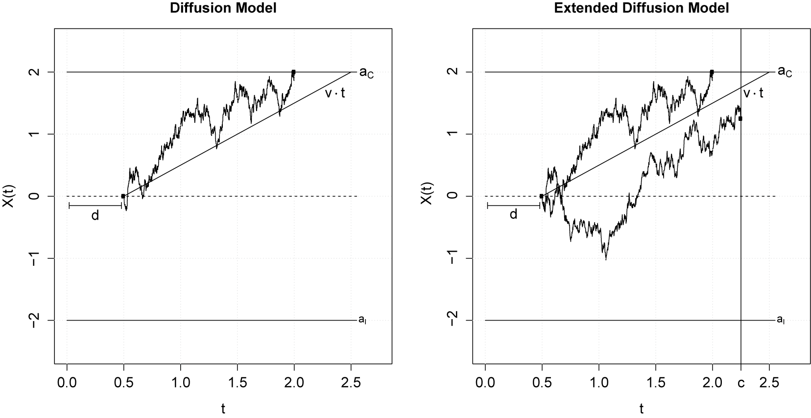


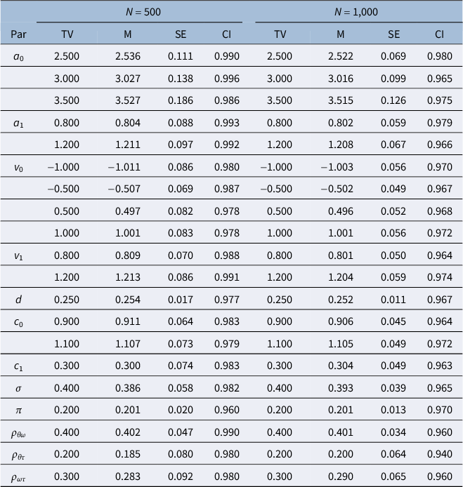
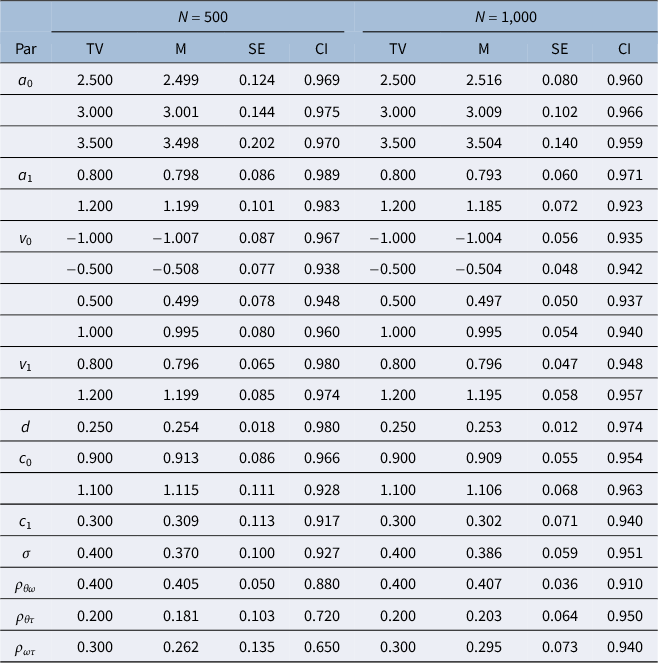

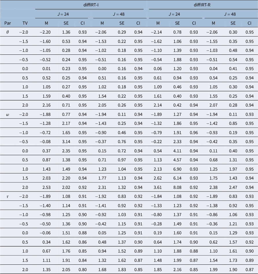
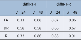
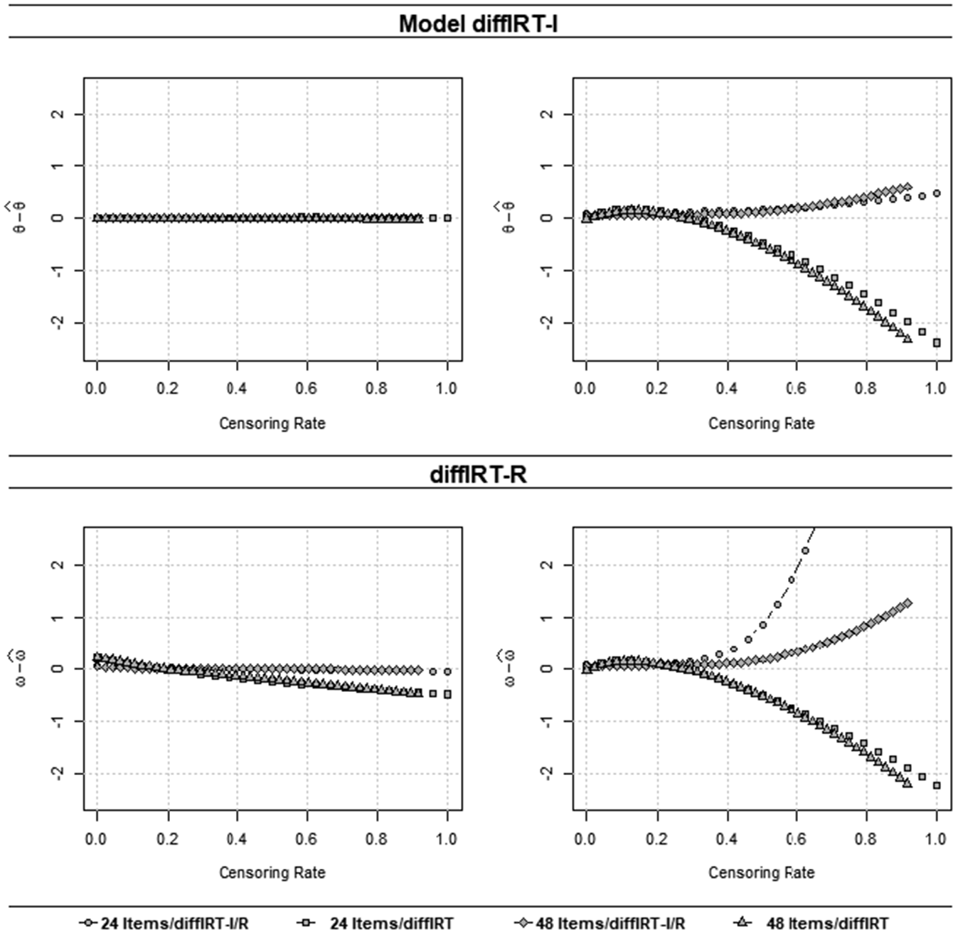


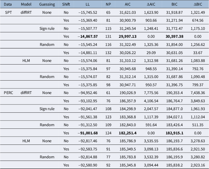


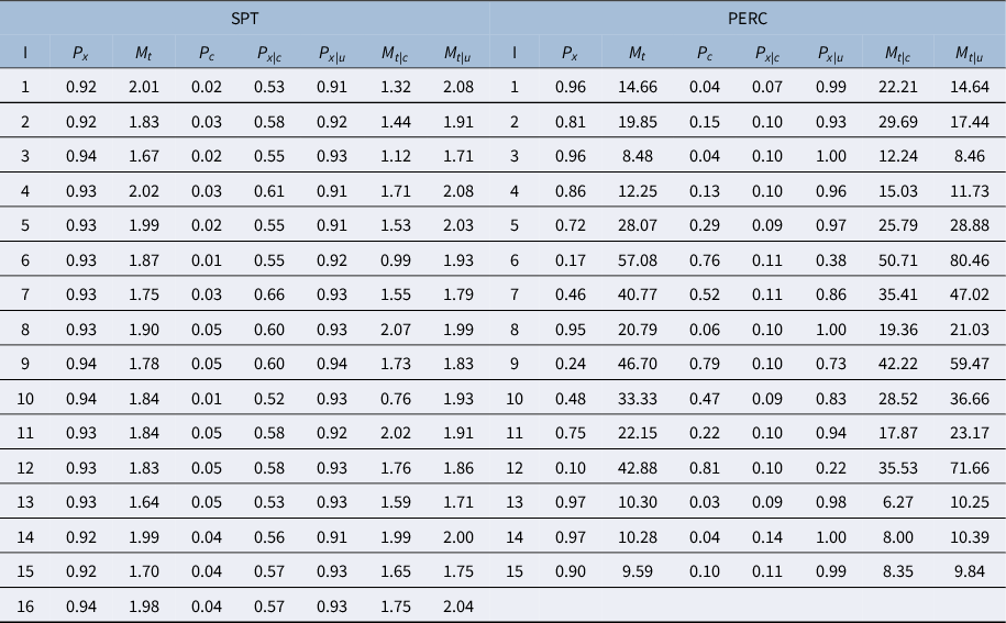


 Open access

