





Introduction
Conservation biocontrol, the promotion of natural enemies of crop pests through land management, can contribute substantially to pest suppression (Symondson et al., Reference Symondson, Sunderland and Greenstone2002; Tschumi et al., Reference Tschumi, Ekroos, Hjort, Smith and Birkhofer2018). Whilst it effectively suppresses disease vectors and crop herbivores (Moore et al., Reference Moore, Borer and Hosseini2010; Michalko et al., Reference Michalko, Pekár, Dul’a and Entling2019), inefficiencies in conservation biocontrol arise through the predation of fellow natural enemies of crop pests (Davey et al., Reference Davey, Vaughan, Andrew King, Bell, Bohan, Bruford, Holland and Symondson2013; Cuff et al., Reference Cuff, Tercel, Drake, Vaughan, Bell, Orozco‐terWengel, Müller and Symondson2022) and other beneficial invertebrates, such as pollinators (Rosenheim et al., Reference Rosenheim, Kaya, Ehler, Marois and Jaffee1995; Hodge, Reference Hodge1999; Tschumi et al., Reference Tschumi, Ekroos, Hjort, Smith and Birkhofer2018). These foraging decisions are usually motivated by complex interactions between biotic drivers, such as the need to redress nutritional deficits (Mayntz et al., Reference Mayntz, Raubenheimer, Salomon, Toft and Simpson2005), and abiotic drivers, such as the management and cycling of crops (Cuff et al., Reference Cuff, Drake, Tercel, Stockdale, Orozco‐terWengel, Bell, Vaughan, Müller and Symondson2021). To optimise the biocontrol activity of natural enemies of crop pests, we must understand how agricultural management decisions, including the myriad changes that arable land progresses through across the annual cycle, affect natural enemy populations and the drivers of their interactions with pests, including nutritional status (Cuff, Gajski et al., Reference Cuff, Gajski, Michalko, Košulič and Pekár2024). From harvest practices (Opatovsky and Lubin, Reference Opatovsky and Lubin2012; Cuff et al., Reference Cuff, Drake, Tercel, Stockdale, Orozco‐terWengel, Bell, Vaughan, Müller and Symondson2021), through tillage (Heimbach and Garbe, Reference Heimbach and Garbe1996; Jowett et al., Reference Jowett, Milne, Garrett, Potts, Senapathi and Storkey2021), to the timing of sowing (Douglas et al., Reference Douglas, Vickery and Benton2010), management decisions can have profound, yet poorly characterised, implications for conservation biocontrol (Cuff, Gajski et al., Reference Cuff, Gajski, Michalko, Košulič and Pekár2024).
The season within which crops are sown can greatly impact their management and productivity; for example, spring-sown crops can see improved disease delay relative to winter-sown crops (Landa et al., Reference Landa, Navas-cortés and Jiménez-díaz2004). As a result, land managers have developed a diverse range of crop management strategies and cycles. Such variations in crop management will also manifest in differences in invertebrate community structure and function due to cascading impacts arising from differences in crop developmental stages (Douglas et al., Reference Douglas, Vickery and Benton2010; Hsu et al., Reference Hsu, Ou and Ho2021). Furthermore, it has the potential to impact the interactions between pests and their predators; for example, when crops sown at different times co-occur in an agricultural landscape, spillover of invertebrates and their interactions from one crop to another presents a significant opportunity for the spread of both pests and predators, especially when earlier-sown crops are harvested (Jaworski et al., Reference Jaworski, Thomine, Rusch, Lavoir, Wang and Desneux2023; Cuff, Gajski et al., Reference Cuff, Gajski, Michalko, Košulič and Pekár2024). By modifying invertebrate community structure (Douglas et al., Reference Douglas, Vickery and Benton2010), agricultural management decisions like crop sowing timing can also indirectly impact the nutrients available to and consumed by natural enemies of crop pests by altering crop development and senescence phenology. As crops senesce in their later developmental stages, nutrients are remobilised away from leaf tissues (Gregersen et al., Reference Gregersen, Holm and Krupinska2008), causing foliar herbivores and their predators to migrate or die (Watt, Reference Watt1979). This is likely to have significant fitness consequences for natural enemies of crop pests, as nutritional deficits will alter their development, fecundity, survival, foraging choices and biocontrol potential (Bilde and Toft, Reference Bilde and Toft1997, Reference Bilde and Toft2001; Mayntz et al., Reference Mayntz, Raubenheimer, Salomon, Toft and Simpson2005).
Nutrients are the fundamental currency of trophic interactions, influencing population dynamics, physiology and species distributions, and driving biocontrol and other ecosystem services (Cuff, Evans et al., Reference Cuff, Evans, Vaughan, Wilder, Tercel and Windsor2024; Wilder et al., Reference Wilder, Herzog, Reeves, Knowles and Cuff2025). Disruption to nutrient acquisition can cascade through consumers (Hedlund et al., Reference Hedlund, Griffiths, Christensen, Scheu, Setälä, Tscharntke and Verhoef2004), reducing energy transfer between trophic groups (Rosenblatt, Reference Rosenblatt2018), ultimately disrupting ecosystem service provision. Generalist predators redress nutritional deficits that arise through such perturbations by engaging in nutrient-specific foraging, the selection of prey based on nutrient content, to optimise their nutrient intake, and therefore fitness (Mayntz et al., Reference Mayntz, Raubenheimer, Salomon, Toft and Simpson2005; Jensen et al., Reference Jensen, Mayntz, Toft, Clissold, Hunt, Raubenheimer and Simpson2012). Nutritional differences between prey are therefore important for the choices predators make, the trophic interactions they engage in, and the ecosystem services they provide, and are likely to be sensitive to agricultural land management practices. By understanding how nutritional dynamics drive ecological processes and are driven by human actions, agricultural land management can be optimised to promote the provision of ecosystem services, including conservation biocontrol, by ensuring sufficient nutrients are available to natural enemies (Cuff, Tercel, Vaughan et al., Reference Cuff, Tercel, Vaughan, Drake, Wilder, Bell, Müller, Orozco‐terWengel and Symondson2024).
Here, we investigated how the timing of crop sowing affects the nutrient content of arthropod predators and whether this is driven by alterations to the prey community available to them. We collected arthropod predators and their prey from winter- and spring-sown wheat, and determined predator biochemical macronutrient (carbohydrate, lipid and protein) content. Using multivariate modelling and null network inference, we tested the following hypotheses: (i) invertebrate prey availability will differ between winter- and spring-sown crops; (ii) arthropod predator nutrient content will differ between winter- and spring-sown crops; (iii) differences in predator nutrient content will relate to recent, but not current, prey availability. By elucidating the nutritional consequences of management decisions such as sowing time for arthropod predators, further investigations can guide optimisation of management to safeguard the nutritional status of natural enemies of crop pests to sustain their beneficial action.
Methods
Arthropod collection and identification
Arthropods were collected from Cockle Park (Morpeth, UK; 55°13′00.8′′ N, 1°41′28.7′′ W) in July 2024. Transects were established in a field containing adjacent plots of spring-sown and winter-sown wheat. Three pairs of belt transects were established 20 m apart within each crop, with 4 m between adjacent transects in the spring and winter-sown crops (fig.1). One pitfall trap was set at the centre of each transect (i.e. three per sowing period), filled with soapy water and deployed for 72 h. Pitfall trapping was conducted twice: once nine days prior to individual arthropod collection (to represent past prey availability) and once in parallel with individual arthropod collection (to represent current prey availability). Invertebrates within these traps were filtered in the field using an AeroPress® and stored in 80% ethanol for subsequent morphological identification. Within each transect, hand-searching was conducted for approximately 10 min, which was deemed sufficient to sample arthropods completely from both the ground and vegetation across the full length of the transect. Individual arthropods were collected directly from the ground or vegetation using a pooter. All arthropods found were collected, but, following morphological identification, only those from known natural enemy groups (i.e. Carabidae, Coccinellidae, Linyphiidae, Lithobiomorpha, Staphylinidae) were included in the analyses below, given the objectives of the study.
Experimental design for invertebrate sampling. Paired sampling locations were established 4 m apart in directly adjacent plots of winter- and spring-sown wheat. Created in BioRender. https://BioRender.com/6rd9udt.

Figure 1 Long description
The diagram illustrates an experimental design for invertebrate sampling in adjacent plots of winter-sown and spring-sown wheat. The left side is labeled 'Winter-sown' and shaded in yellow, while the right side is labeled 'Spring-sown' and shaded in green. Three pairs of pitfall traps are depicted as blue circles, each pair positioned 4 meters apart across the boundary between the two plots. The traps are aligned vertically, with each pair separated by a distance of 20 meters along the transect. The transect is represented by a solid pink line running vertically through both plots, with each trap located 5 meters from the transect line. The key at the bottom of the diagram explains the symbols used: a blue circle represents a pitfall trap, a solid pink line indicates a walked transect and a dashed blue line denotes the distance between samples. The distances between traps and transects are marked with dashed blue lines and labeled with measurements of 4 meters, 5 meters and 20 meters, respectively.
Following collection, the arthropods were frozen onsite at −20 °C to preserve their macronutrient contents for subsequent analysis. The samples were transported to the Molecular Diagnostics Facility at Newcastle University for morphological identification and nutritional analysis. Invertebrates were identified to family level or finer resolution using a stereomicroscope and morphological keys (Luff, Reference Luff2007; Barber, Reference Barber2008; Dallimore and Shaw, Reference Dallimore and Shaw2013; Tilling, Reference Tilling2014; Roberts, Reference Roberts2016). Some invertebrates from pitfall traps were, however, identified to order or suborder, where access to appropriate identification resources or damage to specimens limited identification. Individuals from each taxon were then counted to produce species-by-site abundance data.
Macronutrient quantification
Macronutrient analysis followed the Macronutrient Extraction and Determination from Invertebrates method (Cuff et al., Reference Cuff, Drake, Tercel, Stockdale, Orozco‐terWengel, Bell, Vaughan, Müller and Symondson2021; Cuff and Wilder, Reference JP and SM2021), which streamlines sulfo-phospho-vanillin, anthrone and Lowry colourimetric assays for lipid, carbohydrate and protein estimation, respectively. This protocol was, however, adapted for compatibility with 384-well plates to facilitate a greater analysis throughput, with assay volumes adjusted accordingly. To extract macronutrients from whole arthropods, individuals were placed in 2 ml tubes of a 96-well rack and heated until dry (∼1 h) in an oven at 60 °C. To each sample, 500 μl of 1:12 chloroform:methanol solution was added and left at room temperature for 24 h. After 24 h, 400 μl of the chloroform:methanol solution was removed and retained separately for lipid analysis. A further 500 μl of chloroform:methanol solution was added to the sample and incubated at room temperature for 24 h to remove any residual lipids. All chloroform:methanol solution was removed by pipetting, and any residue was evaporated in an oven at 60 °C for ∼15 min.
To each dried sample, 500 μl 0.1 M NaOH was added, after which the samples were incubated at 80 °C for 30 min and at room temperature overnight (∼16 h). The samples were briefly centrifuged (∼2 min, 2,000× g) to avoid taking solid material through to the subsequent assays. From each sample, 400 μl of the supernatant was transferred into a separate tube for protein and carbohydrate determination. All assays were carried out in a 384-well plate format. For each assay, a stock standard dilution series of a known concentration was made with lard oil, glucose and bovine serum albumin (BSA) for lipid, carbohydrate and protein quantification, respectively. Stock solutions of 2 mg ml−1 glucose and BSA were made using distilled water and subsequently diluted in 0.1 M NaOH, whereas 2 mg ml−1 lard oil was made and diluted with 1:12 chloroform:methanol. Dilution series comprised 0–1 mg ml−1 in nine increments (0, 12.5, 62.5, 125, 250, 375, 500, 750, 1,000 μg ml−1). A quarter of each 384-well assay plate (96 wells) was reserved for repeats of these standards.
Lipid quantification
The sulfo-phospho-vanillin method was used to determine lipid content. The vanillin reagent was prepared by mixing 0.108 mg of vanillin with 18 μl of hot water and 72 μl of 85% phosphoric acid for every 100 μl of reagent. From each sample, three repeats of 20 μl were added to a 384-well plate alongside standards and heated to 100 °C for 5 min to evaporate the chloroform:methanol carrier. To each well, 10 μl of concentrated sulfuric acid was added, mixed briefly on a plate shaker and incubated at room temperature for 15 min. Following this, 75 μl of vanillin reagent was added to each well, mixed briefly on a plate shaker and incubated at room temperature for 10 min. Absorbance at 490 nm for each was determined in a spectrophotometer.
Carbohydrate quantification
The anthrone method was used to determine carbohydrate content. The anthrone reagent was prepared by mixing 100 μg of anthrone with 100 μl of concentrated sulfuric acid for every 100 μl of reagent. From each sample, three repeats of 20 μl were added to a 384-well plate alongside standards, mixed with 80 μl of the anthrone reagent and incubated at 92 °C for 10 min. The plate was incubated at room temperature for 5 min, and absorbance at 620 nm for each well was determined in a spectrophotometer.
Protein quantification
The Lowry method was used to determine protein content. From each sample, three repeats of 20 μl were added to a 384-well plate alongside standards, and 60 μl of modified Lowry reagent was added to each well and mixed briefly on a plate shaker. The plate was incubated at room temperature for 10 min, and 6 μl of 1X Folin-Ciocalteu reagent was added and mixed briefly on a plate shaker. The plate was incubated at room temperature for 30 min, and absorbance at 750 nm for each well was determined in a spectrophotometer.
Statistical analysis
All analyses were conducted in R version 4.5.2 (R Core Team, 2025) and all data processing used the ‘tidyverse’ package for reproducibility (Wickham et al., Reference Wickham, Averick, Bryan, Chang, D’Agostino, François, Grolemund, Hayes, Henry, Hester, Kuhn, Lin Pedersen, Miller, Milton, Müller, Ooms, Robinson, Seidel, Spinu, Takahashi, Vaughan, Wilke, Woo and Yutani2019). Data visualisations were generated using ggplot2 (Wickham, Reference Wickham2016).
The pitfall-trapped invertebrate communities (herein considered representative of prey available to the hand-collected arthropod predators) were compared between winter- and spring-sown crops, pitfall trapping rounds and an interaction between the two using multivariate generalised linear models (MGLMs) with a Poisson error family and Monte Carlo resampling in the ‘mvabund’ package via the ‘manyglm’ function (Wang et al., Reference Wang, Naumann, Wright and Warton2012). These differences were visualised using non-metric multidimensional scaling with a Bray-Curtis dissimilarity matrix in the ‘vegan’ package (Oksanen et al., Reference Oksanen, Simpson, Blanchet, Kindt, Legendre, Minchin, O’hara, Solymos, Stevens, Szoecs, Wagner, Barbour, Bedward, Bengtsson, Bolker, Borcard, Borman, Carvalho, Chirico, De Caceres, Durand, Evangelista, FitzJohn, Friendly, Furneaux, Hannigan, Heida, Hill, Lahti, Martino, McGlinn, Ouellette, Cunha, Smith, Stier, Ter Braak and Weedon2022). Square-root-transformed macronutrient contents (i.e. percentage total macronutrient mass for each macronutrient) of arthropods were compared between taxa (based on the finest taxonomic resolution available for each predator taxon, mostly genus-level), winter- and spring-sown crops and the interaction between the two using multivariate linear models (MLMs) in the ‘mvabund’ package via the ‘manylm’ function (Wang et al., Reference Wang, Naumann, Wright and Warton2012). Due to some taxa being present in only one of the two crops or fewer than three individuals being present overall, Coccinella septempunctata, Loricera pilicornis, Patrobus atrorufus, Lamyctes emarginatus and Anchomenus dorsalis were aggregated as ‘other’ for this comparison of nutrient content.
Null network models were run to infer density-dependent interactions for each of the individually collected arthropod predators based on prey availability and to determine if prey availability explains differences in predator nutrient content. Using pitfall trapping prey availability data, separately for the past and present prey availability based on the two rounds of pitfall trapping, null networks were generated for each of the individually collected predators included in the nutritional analyses above. These null network models assume that the trophic interactions of the predators were density-dependent (i.e. they interacted with the prey most available to them), providing a semi-realistic estimate of how prey availability would translate to trophic interactions.
To construct null networks, null diets were simulated using the ‘generate_null_net’ function in the ‘econullnetr’ package (Vaughan et al., Reference Vaughan, Gotelli, Memmott, Pearson, Woodward and Symondson2018) using the prey availability data from the pitfall traps with random placeholder interaction data. To generate null networks, we required dummy interaction data. We simulated these dummy interactions for each individual arthropod predator by randomly allocating interactions with three of the available prey taxa (approximately reflecting the interaction richness of arable arthropod predators from previous work; Cuff et al., Reference Cuff, Tercel, Drake, Vaughan, Bell, Orozco‐terWengel, Müller and Symondson2022). These dummy data were only required to run null network simulations and did not otherwise feature in any downstream analyses, with the exception of the fact that the node degree is invariable (i.e. a mean of three interactions per predator across all simulations). Using the ‘generate_null_net_indiv’ function (Cuff et al., Reference Cuff, Windsor, Tercel, Bell, Symondson and Vaughan2023), only the simulation data were extracted irrespective of the identities of the random interaction data input. Null networks were visually constructed using ‘igraph’ (Csardi and Nepusz, Reference Csardi and Nepusz2006) and plotted using ‘ggnetwork’ (Briatte, Reference Briatte2021). Null network-inferred predator-prey interactions based on both past and present prey availability were compared against predator nutrient content using redundancy analysis (RDA), and model outputs were analysed using analysis of variance (ANOVA) of the overall model, terms within the model and model axes.
Results
From the six transects, nutritional data were generated for 98 hand-collected predatory arthropods (Supplementary Table S1), 52 from the winter-sown wheat, and 46 from the spring-sown wheat. These belonged to five families: Carabidae (n = 86), Coccinellidae (2), Henicopidae (3), Linyphiidae (3) and Staphylinidae (4; Supplementary Table S1). The pitfall traps collected 668 individual invertebrates across 28 taxa resolved to family (n = 22), suborder (n = 1) or order level (n = 5; Supplementary Table S2), considered representative of prey available to the above predatory arthropods. These taxa included common wheat pests (n = 4), detritivores (n = 7) and natural enemies of crop pests (n = 10).
A significant overall effect on prey community abundances related to sowing period and sampling round was identified (MGLM: Wald = 13.89, p = 0.001), specifically related to carabid beetles (MGLM: Wald = 6.276, p = 0.001), linyphiid spiders (MGLM: Wald = 6.709, p = 0.001) and platygastrid wasps (MGLM: Wald = 8.312, p = 0.001). Sequential multivariate ANOVA identified significant marginal effects of crop sowing period (MGLM: Dev = 213.55, df = 10, p = 0.001; fig. 2), sampling round (MGLM: Dev = 133.33, df = 9, p = 0.001) and the interaction between sowing period and sampling round (MGLM: Dev = 42.98, df = 8, p = 0.001). Specifically, the abundances of brachyceran flies (MGLM: Dev = 20.794, df = 10, p = 0.001), carabid beetles (MGLM: Dev = 28.456, df = 10, p = 0.001), ichneumonid wasps (MGLM: Dev = 8.662, df = 10, p = 0.046), linyphiid spiders (MGLM: Dev = 23.599, df = 10, p = 0.001), platygastrid wasps (MGLM: Dev = 83.939, df = 10, p = 0.001) and stratiomyid flies (MGLM: Dev = 9.704, df = 10, p = 0.034) differed between crops sown in winter and spring. Similarly, the abundances of brachyceran flies (MGLM: Dev = 20.794, df = 9, p = 0.001), carabid beetles (MGLM: Dev = 9.272, df = 9, p = 0.044), linyphiid spiders (MGLM: Dev = 31.662, df = 9, p = 0.001) and stratiomyid flies (MGLM: Dev = 9.704, df = 9, p = 0.044) differed between pitfall trapping rounds. No significant taxon-specific relationships were identified for the interaction between sowing period and pitfall trapping round. Coefficient-level tests also demonstrated that prey community abundances related to sowing period (MGLM: Wald = 6.948, p = 0.001; fig. 2), sampling round (MGLM: Wald = 6.062, p = 0.001) and the interaction between sowing period and sampling round (MGLM: Dev = 3.642, p = 0.018). Specifically, the abundances of linyphiid spiders (MGLM: Wald = 3.827, p = 0.002) and platygastrid wasps (MGLM: Wald = 4.079, p = 0.001) significantly differed between sowing periods. Similarly, the abundances of carabid beetles (MGLM: Wald = 3.330, p = 0.001) differed between sampling rounds, and the abundances of platygastrid wasps related to an interaction between sowing period and sampling round (MGLM: Wald = 2.475, p = 0.046).
Non-metric multidimensional scaling of arthropod prey communities available in spring-sown (n = 6) and winter-sown (n = 6) wheat (left), and between pitfall trapping rounds (right; n = 6 per round). Stress = 0.103.
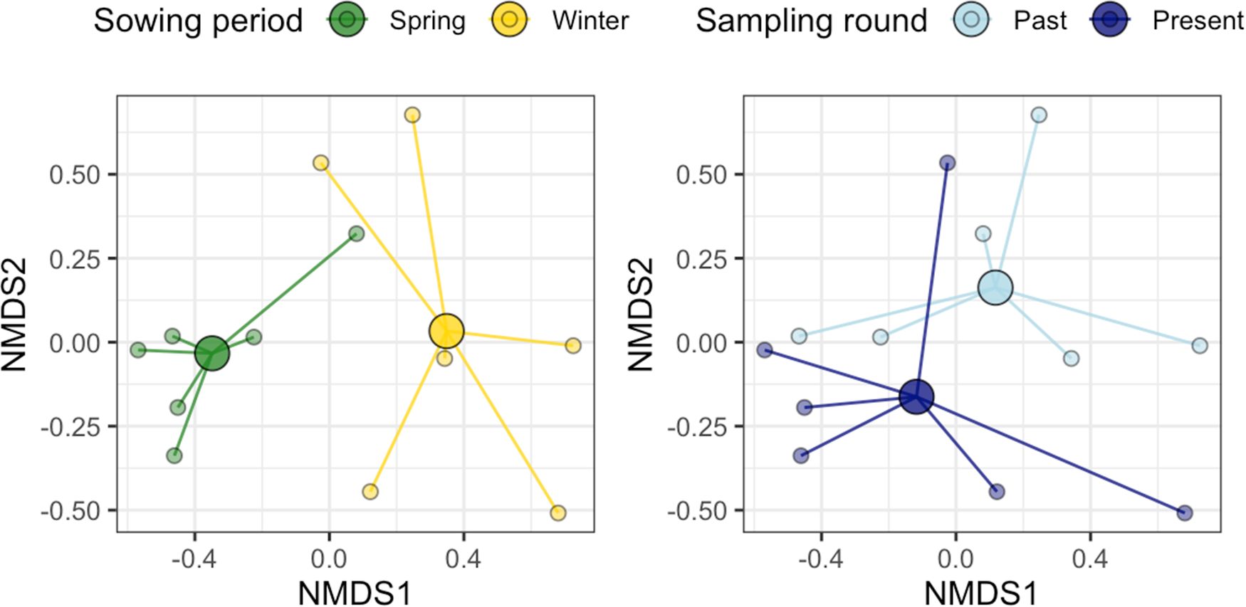
Figure 2 Long description
The left scatter plot represents the sowing period with categories 'Spring' and 'Winter'. The horizontal axis is labeled 'NMDS1' and the vertical axis is labeled 'NMDS2'. NMDS1 ranges from approximately negative 0.5 to 0.5 and NMDS2 ranges from approximately negative 0.5 to 0.6. Points are clustered around larger centroid-like markers, with lines connecting these centroids to individual samples. The 'Spring' group is more dispersed, while the 'Winter' group shows tighter clustering, indicating separation along NMDS1 and NMDS2. The right scatter plot represents the sampling round with categories 'Past' and 'Present'. The axes are similarly labeled 'NMDS1' and 'NMDS2', with the same approximate ranges. Points are connected to larger centroid-like markers, illustrating trajectories or group centroids. The 'Past' group shows more dispersion compared to the 'Present' group, indicating distinct separation between the two categories. The plots aim to show differences in community structure based on sowing period and sampling round, with notable separation and varying dispersion between groups.
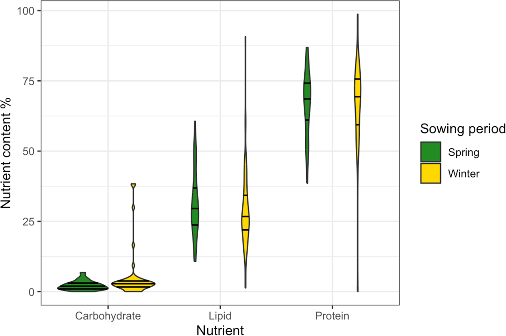
A significant overall effect of sowing period and taxon on predatory arthropod nutrient contents was identified (MLM: Lawley–Hotelling trace = 5.614, p = 0.014), specifically on carbohydrates (MLM: F = 1.629, p = 0.036), lipids (MLM: F = 2.888, p = 0.013) and proteins (MLM: F = 1.097, p = 0.046). Sequential multivariate ANOVA identified no significant marginal effects of crop sowing period (MLM: F 1,96 = 5.265, p = 0.189; fig. 3), taxon (MLM: F 5,91 = 6.141, p = 0.069), or their interaction (MLM: F 5,86 = 4.788, p = 0.156), with no significant underlying univariate relationships. Coefficient-level tests did, however, demonstrate that predator nutrient contents related to sowing period (MGLM: Wald = 9.847, p = 0.006; fig. 3), alongside specific taxon effects and the interaction between specific taxa and sowing periods. The proportional content of carbohydrate (MLM: F = 9.119, p = 0.002) significantly differed between crops sown in winter and spring, with carbohydrate being proportionally higher in winter-sown crops. Lipid (MLM: F = 0.223, p = 0.104) and protein (MLM: F = 0.504, p = 0.098) content did not significantly differ between sowing periods, although all three macronutrients were more variable in their content in winter-sown crops.
Violin plot of proportional macronutrient content (carbohydrate, lipid, protein) of predatory arthropods collected from winter-sown (n = 52) and spring-sown (n = 46) wheat. Horizontal lines within each violin represent the median and quartiles.

Figure 3 Long description
The horizontal axis label is Nutrient. The categories are Carbohydrate, Lipid, Protein. The vertical axis label is Nutrient content percent. The range is 0 to 100. A legend label reads Sowing period, with entries Spring and Winter. Carbohydrate has two violins, Spring and Winter. The Spring violin is concentrated near 0 to about 10. The Winter violin is concentrated near 0 to about 10, with several separate points above the main shape at about 15, about 20, about 30 and about 35. Lipid has two violins, Spring and Winter. The Spring violin spans from about 15 to about 60, with the widest section around about 25 to about 35. The Winter violin spans from about 0 to about 90, with the widest section around about 20 to about 35. Protein has two violins, Spring and Winter. The Spring violin spans from about 40 to about 90, with the widest section around about 65 to about 80. The Winter violin spans from about 0 to about 100, with the widest section around about 60 to about 85. Each violin contains horizontal lines marking the median and quartiles.
Null network predator–prey interactions did not significantly explain predator nutrient contents when considering past (RDA: F = 0.851, df = 19, p = 0.673; fig. 4) nor present (RDA: F = 0.864, df = 24, p = 0.656; fig. 4) prey availability, and most individual model terms (prey) did not significantly explain predator nutrient content, although there was a marginally insignificant relationship between past Keroplatidae abundance and predator nutrient contents (ANOVA: F = 2.686, df = 1, p = 0.089), and significant and marginally insignificant relationships involving present Collembola (ANOVA: F = 6.361, df = 1, p = 0.013) and Braconidae (ANOVA: F = 2.662, df = 1, p = 0.096) abundances, respectively.
Inferred networks of predator-prey interactions based on prey availability for spring wheat (green prey nodes) and winter wheat (yellow prey nodes) based on data taken nine days before (‘past’; light blue links) and in parallel with samples used for nutritional analysis (‘present’; dark blue links). Upper nodes are predators when present nutrient data given with yellow, blue and red denoting carbohydrate, lipid, and protein proportional content, respectively.
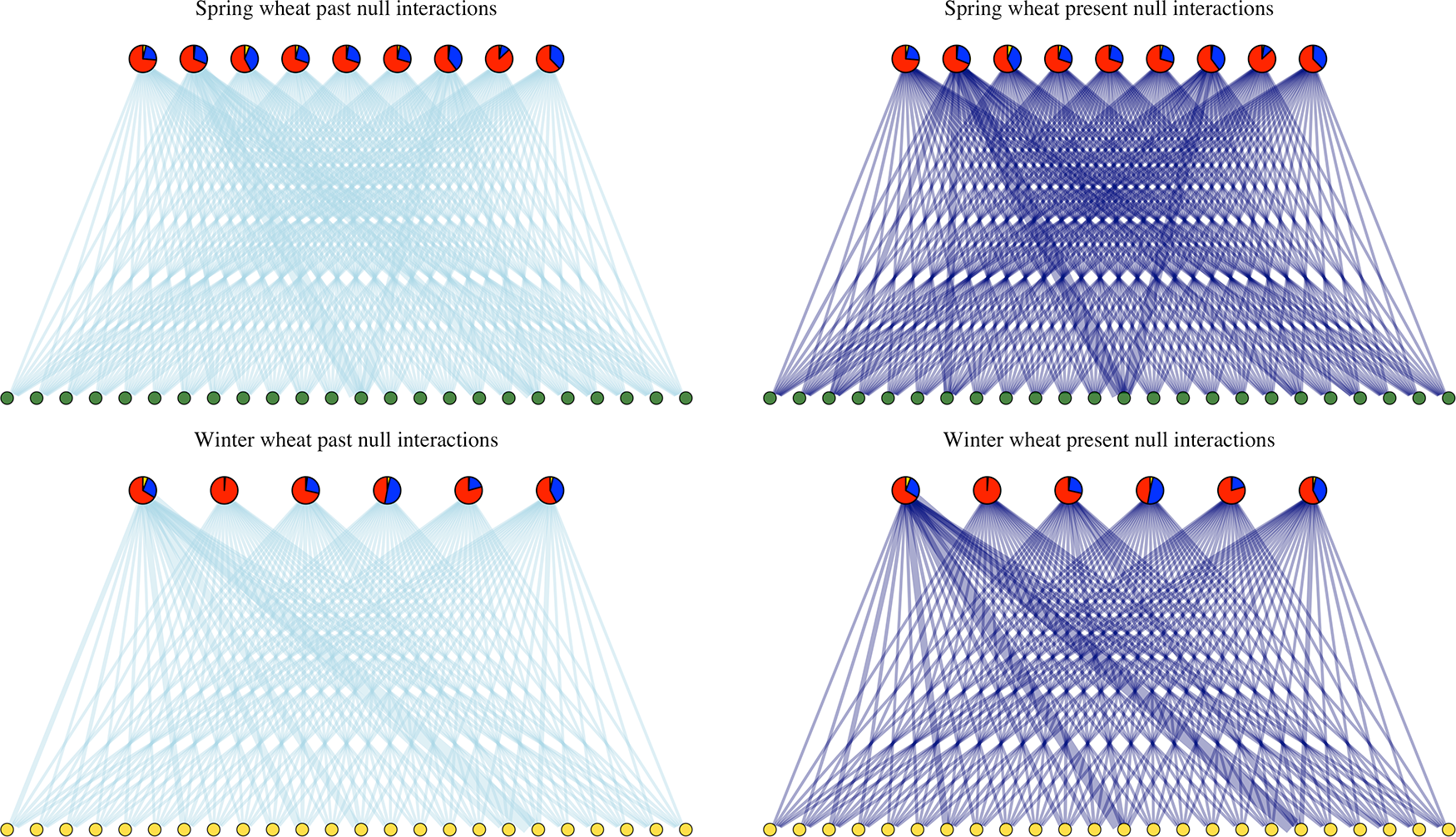
Figure 4 Long description
The image consists of four diagrams illustrating inferred networks of predator-prey interactions based on prey availability for spring and winter wheat. The top left diagram is labeled 'Spring wheat past null interactions' and features light blue links connecting upper predator nodes to lower green prey nodes. The top right diagram, labeled 'Spring wheat present null interactions,' shows dark blue links connecting the same predator nodes to prey nodes, indicating present interactions. The bottom left diagram, labeled 'Winter wheat past null interactions,' displays light blue links connecting upper predator nodes to lower yellow prey nodes. The bottom right diagram, labeled 'Winter wheat present null interactions,' features dark blue links connecting the same predator nodes to prey nodes, representing present interactions. The upper nodes are colored with yellow, blue and red, denoting carbohydrate, lipid and protein proportional content, respectively.
Discussion
The nutrient content of arthropod predators was associated with the timing of crop sowing, even across the small spatial scales used in this study (i.e. parallel transects 4 m apart). Whilst the prey available to those predators also changed across those small spatial scales, neither current nor recent prey availability explained the nutritional differences. This could indicate density-independent foraging of the arthropod predators (i.e. foraging for prey disproportionate to their availability, observed in similar predatory assemblages; Cuff et al., Reference Cuff, Tercel, Drake, Vaughan, Bell, Orozco‐terWengel, Müller and Symondson2022), or a shift in prey quality, irrespective of taxonomic identity, associated with differences in the developmental stage of crops sown in winter and spring. The crops themselves will likely differ markedly in their nutrient content at different developmental stages given the remobilisation of nutrients away from leaf tissue over time (Gregersen et al., Reference Gregersen, Holm and Krupinska2008). This will possibly have concomitant impacts on the herbivorous insects feeding on them, which are then predated by the focal arthropod predators of this study. The greater variability in nutrient content in predators from the winter-sown wheat, for example, could relate to the scarcity of nutrients in the senescing wheat relative to the younger wheat in the spring-sown crop. Senescing crops can drive the death or dispersal of foliar herbivores and their predators (Watt, Reference Watt1979), likely resulting in nutritional variation and decline in those that remain. Prey quality, rather than availability, may therefore be the primary driver of the observed nutritional differences (Wilder et al., Reference Wilder, Mayntz, Toft, Rypstra, Pilati and Vanni2010; Schmidt et al., Reference Schmidt, Sebastian, Wilder and Rypstra2012; Rendon et al., Reference Rendon, Taylor, Wilder and Whitehouse2019). Since prey nutrient content influences the nutrition and trophic interactions of predators (Wilder et al., Reference Wilder, Barnes and Hawlena2019; Cuff, Tercel, Vaughan et al., Reference Cuff, Tercel, Vaughan, Drake, Wilder, Bell, Müller, Orozco‐terWengel and Symondson2024), this could indicate a nutritional cascade from the crop as a basal resource to the arthropod predators, although this requires further investigation in a larger-scale study.
This hypothetical nutritional cascade could have important implications for subsequent biocontrol and the spillover of arthropods and interactions from winter- to spring-sown crops continuously and particularly following harvest. The greater nutritional variation in predators in the winter-sown wheat could indicate increased rates of nutritional imbalance, which would then be likely redressed through nutrient-specific foraging as they migrate to other crops (Mayntz et al., Reference Mayntz, Raubenheimer, Salomon, Toft and Simpson2005). Given the larger variation in nutrient contents of winter-sown wheat predators, it may be harder to predict the interactions and nutritional dynamics of these predators as they migrate to other locations, such as spring-sown crops. Harvest of winter-sown crops, which will increase community turnover through physical disturbance (Opatovsky and Lubin, Reference Opatovsky and Lubin2012; Cuff et al., Reference Cuff, Drake, Tercel, Stockdale, Orozco‐terWengel, Bell, Vaughan, Müller and Symondson2021), is likely to propagate this migration through spillover, especially between adjacent plots (Cuff, Gajski et al., Reference Cuff, Gajski, Michalko, Košulič and Pekár2024).
This work was intentionally carried out at a small spatial scale, with only 4 m separating the transects in winter- and spring-sown crops. The intention was to determine either that differences could be resolved at such small spatial scales, or that arthropods were spilling over between the two adjacent crops. Whilst a significant difference in nutrient content was detected at this resolution, this was not consistent across analyses, and spillover is likely nonetheless, especially given that many of the arthropod predators studied are mobile. Most of the predators collected were small ground beetles such as Bembidion spp., the foraging range of which is poorly characterised; however, other larger ground beetles are known to travel less than 1 m per day (Schreiner and Irmler, Reference Schreiner and Irmler2009). This could imply that the ‘present’ prey availability data were representative of their recent prey availability, even if the ‘past’ prey availability data were less likely to be representative. That some significant difference in nutrient content was observed could support the notion that the difference between the two crop stages resulted in the divergent nutritional states of predators. Alternatively, the nutritional state of the predators could have driven them to forage in a specific crop stage, seeking nutrients that were deficient in the other crop stage. The latter would be consistent with optimal foraging theory if each ‘patch’ presented different nutritional opportunities (Pyke et al., Reference Pyke, Pulliam and Charnov1977). Both eventualities do, however, indicate a nutritional effect of crop developmental stage with implications for wider foraging, predator fitness and biocontrol, which requires further investigation.
This study was a brief snapshot of a potentially complex and continuously evolving dynamic between crop development and predator nutrition. Given the indirect link between predators and crops, other nutrients, including elemental macronutrients and micronutrients, may be important drivers of interactions (Kaspari, Reference Kaspari2021; Wilder et al., Reference Wilder, Herzog, Reeves, Knowles and Cuff2025). This study provides the foundations from which to investigate this dynamic deeper, ideally by linking nutrient flow through each trophic level to determine how nutrients structure the wider ecological system (Cuff, Evans et al., Reference Cuff, Evans, Vaughan, Wilder, Tercel and Windsor2024). Whilst the interactions inferred based on prey availability data are likely to reflect the pool of prey accessible to the predators studied and null models can generate semi-accurate interaction data (Cuff, Tercel, Windsor et al., 2024), trophic interactions are often density-independent (Vaughan et al., Reference Vaughan, Gotelli, Memmott, Pearson, Woodward and Symondson2018; Cuff et al., Reference Cuff, Tercel, Drake, Vaughan, Bell, Orozco‐terWengel, Müller and Symondson2022; Gajski et al., Reference Gajski, Mifková, Košulič, Michálek, Serbina, Michalko and Pekár2024), the deviations of which from our models are unknown. The interactions inferred should therefore be interpreted with caution, and future investigations should identify trophic interactions empirically.
Conclusions
We have demonstrated that, at least in this small-scale snapshot study, the nutrient contents of arthropod predators can change with the sowing period of crops on even very small spatial scales. Whilst prey availability concomitantly changes, it does not explain this nutritional variation, possibly indicating a more complex set of mechanisms, potentially relating to cascading impacts to the nutritional quality of prey as a result of different stages of crop development and senescence. That basal resource quality could underpin predator nutritional fitness through trophic cascades has important implications for the management of crops to sustain healthy natural enemy populations. This is likely to be particularly relevant in monocultural arable systems where alternative basal resources are scarce if available at all. The potential spillover of nutritionally distinct predator and pest populations from winter- to spring-sown crops, either continuously or following harvest, has the potential to rewire nutritional networks in adjacent spring-sown crops. This study provides the foundations for further investigation of this crucial nutritional dynamic, ideally with greater replication across a broader range of contexts to enable greater generalisability of the results. Expansion of the spatiotemporal scope of this study could identify novel management strategies to optimise natural enemy population health and conservation biocontrol.
Supplementary material
The supplementary material for this article can be found at https://doi.org/10.1017/S000748532610114X.
Acknowledgements
The authors are extremely grateful to the editorial team of Bulletin of Entomological Research and Gwenaëlle Deconninck for constructive comments during the peer review process. For the purpose of open access, the authors have applied a Creative Commons Attribution (CC-BY) licence to any Author Accepted Manuscript version arising from this submission. Generative AI (ChatGPT) was used for grammatical checks on an initial draft of the manuscript, which was subsequently checked and edited by all co-authors. Generative AI was also used for error-checking and refinement of initial data analysis scripts in R.
Author contributions
R.C.: data curation, formal analysis, investigation, methodology, visualisation, writing – review and editing. R.W.: conceptualisation, data curation, formal analysis, investigation, methodology, visualisation, writing – original draft. F.M.W.: investigation, methodology, project administration, supervision, writing – review and editing. J.P.C.: conceptualisation, data curation, formal analysis, investigation, methodology, project administration, supervision, visualisation, writing – review and editing. R.C. and R.S.W. contributed equally to this work.
Financial support
R.C. and J.P.C. were funded by a Newcastle University Academic Track Fellowship.
Competing interests
None to declare.
Data availability
All data and code are openly available via Zenodo: https://doi.org/10.5281/zenodo.17911631.



 Open access

