


1. Introduction
The Ly
 $\alpha$
emission (
$\alpha$
emission (
 $1\,215.67$
Å) line of hydrogen atom is a key spectral feature that is used to detect and study high-redshift galaxies (e.g. Dijkstra Reference Dijkstra2014; Hayes Reference Hayes2015; Ouchi, Ono, & Shibuya Reference Ouchi, Ono and Shibuya2020). Due to their resonant nature, Ly
$1\,215.67$
Å) line of hydrogen atom is a key spectral feature that is used to detect and study high-redshift galaxies (e.g. Dijkstra Reference Dijkstra2014; Hayes Reference Hayes2015; Ouchi, Ono, & Shibuya Reference Ouchi, Ono and Shibuya2020). Due to their resonant nature, Ly
 $\alpha$
photons scatter frequently in the interstellar, circumgalactic, and even intergalactic medium (ISM, CGM, and IGM, respectively). This random walk leads to a wide diversity of spectral shapes of Ly
$\alpha$
photons scatter frequently in the interstellar, circumgalactic, and even intergalactic medium (ISM, CGM, and IGM, respectively). This random walk leads to a wide diversity of spectral shapes of Ly
 $\alpha$
that contain information about the kinematics and geometry of the gas present in ISM and CGM (see Dijkstra et al. Reference Dijkstra, Prochaska, Ouchi and Hayes2019 for a review). The characteristic shape of Ly
$\alpha$
that contain information about the kinematics and geometry of the gas present in ISM and CGM (see Dijkstra et al. Reference Dijkstra, Prochaska, Ouchi and Hayes2019 for a review). The characteristic shape of Ly
 $\alpha$
emission, making it easily recognisable, is typically a single red asymmetric line profile (e.g. Shapley et al. Reference Shapley, Steidel, Pettini and Adelberger2003; Tapken et al. Reference Tapken2007). However, over the past decade, double-peaked profiles of Ly
$\alpha$
emission, making it easily recognisable, is typically a single red asymmetric line profile (e.g. Shapley et al. Reference Shapley, Steidel, Pettini and Adelberger2003; Tapken et al. Reference Tapken2007). However, over the past decade, double-peaked profiles of Ly
 $\alpha$
, characterised by two asymmetric peaks, have been detected in both local galaxies (e.g. Jaskot & Oey Reference Jaskot and Oey2014; Henry et al. Reference Henry, Scarlata, Martin and Erb2015; Verhamme et al. Reference Verhamme2017; Orlitová et al. Reference Orlitová2018; Izotov et al. Reference Izotov2018) and galaxies out to high redshifts (i.e.
$\alpha$
, characterised by two asymmetric peaks, have been detected in both local galaxies (e.g. Jaskot & Oey Reference Jaskot and Oey2014; Henry et al. Reference Henry, Scarlata, Martin and Erb2015; Verhamme et al. Reference Verhamme2017; Orlitová et al. Reference Orlitová2018; Izotov et al. Reference Izotov2018) and galaxies out to high redshifts (i.e.
 $z = 2 - 7$
; Kulas et al. Reference Kulas2012; Yamada et al. Reference Yamada2012; Matthee et al. Reference Matthee2018; Hayes et al. Reference Hayes, Runnholm, Gronke and Scarlata2021; Meyer et al. Reference Meyer, Laporte, Ellis, Verhamme and Garel2021; Songaila et al. Reference Songaila, Barger, Cowie, Hu and Taylor2022; Erb et al. Reference Erb2023; Moya-Sierralta et al. Reference Moya-Sierralta2024; Vitte et al. Reference Vitte2025). Double-peaked profiles are also detected in Lyman alpha nebulae, or blobs (Yang et al. Reference Yang, Zabludoff, Jahnke and Davé2014; Vanzella et al. Reference Vanzella2017; Li et al. Reference Li, Steidel, Gronke, Chen and Matsuda2022), suggesting complex radiative transfer effects and the presence of large-scale gas kinematics. In addition, a few triple-peaked profiles have also been reported (e.g. Rivera-Thorsen et al. Reference Rivera-Thorsen2017; Vanzella et al. Reference Vanzella2018; Vitte et al. Reference Vitte2025). The Multi-Unit Spectroscopic Explorer (MUSE) at the Very Large Telescope (VLT; Bacon et al. Reference Bacon, McLean, Ramsay and Takami2010), has revealed a vast population of Ly
$z = 2 - 7$
; Kulas et al. Reference Kulas2012; Yamada et al. Reference Yamada2012; Matthee et al. Reference Matthee2018; Hayes et al. Reference Hayes, Runnholm, Gronke and Scarlata2021; Meyer et al. Reference Meyer, Laporte, Ellis, Verhamme and Garel2021; Songaila et al. Reference Songaila, Barger, Cowie, Hu and Taylor2022; Erb et al. Reference Erb2023; Moya-Sierralta et al. Reference Moya-Sierralta2024; Vitte et al. Reference Vitte2025). Double-peaked profiles are also detected in Lyman alpha nebulae, or blobs (Yang et al. Reference Yang, Zabludoff, Jahnke and Davé2014; Vanzella et al. Reference Vanzella2017; Li et al. Reference Li, Steidel, Gronke, Chen and Matsuda2022), suggesting complex radiative transfer effects and the presence of large-scale gas kinematics. In addition, a few triple-peaked profiles have also been reported (e.g. Rivera-Thorsen et al. Reference Rivera-Thorsen2017; Vanzella et al. Reference Vanzella2018; Vitte et al. Reference Vitte2025). The Multi-Unit Spectroscopic Explorer (MUSE) at the Very Large Telescope (VLT; Bacon et al. Reference Bacon, McLean, Ramsay and Takami2010), has revealed a vast population of Ly
 $\alpha$
emitters (LAEs) with diverse spectral profiles at redshifts
$\alpha$
emitters (LAEs) with diverse spectral profiles at redshifts
 $z = 2.9$
–
$z = 2.9$
–
 $6.7$
(see Herenz et al. Reference Herenz2017; Bacon et al. Reference Bacon2023; Vitte et al. Reference Vitte2025). Meanwhile, the Near Infrared Spectrograph aboard the James Webb Space Telescope (JWST/NIRSpec) is already extending the boundaries of Ly
$6.7$
(see Herenz et al. Reference Herenz2017; Bacon et al. Reference Bacon2023; Vitte et al. Reference Vitte2025). Meanwhile, the Near Infrared Spectrograph aboard the James Webb Space Telescope (JWST/NIRSpec) is already extending the boundaries of Ly
 $\alpha$
line observations to even higher redshifts (Bunker et al. Reference Bunker2024).
$\alpha$
line observations to even higher redshifts (Bunker et al. Reference Bunker2024).
Double-peaked Ly
 $\alpha$
profiles typically arise due to scattering of photons from a static or expanding/infalling medium of neutral hydrogen cloud, which shifts their frequencies away from the line center and produces two peaks. In an outflowing medium, photons preferentially escape on the red side, producing a dominant red peak with a weaker blue bump. Additionally, Ly
$\alpha$
profiles typically arise due to scattering of photons from a static or expanding/infalling medium of neutral hydrogen cloud, which shifts their frequencies away from the line center and produces two peaks. In an outflowing medium, photons preferentially escape on the red side, producing a dominant red peak with a weaker blue bump. Additionally, Ly
 $\alpha$
photons can backscatter off a receding outflow on the far side of the galaxy, which shifts their frequency out of resonance and allows them to escape without further scatterings (Dijkstra, Haiman, & Spaans Reference Dijkstra, Haiman and Spaans2006; Verhamme, Schaerer, & Maselli Reference Verhamme, Schaerer and Maselli2006; Steidel et al. Reference Steidel2010), while multiple backscattering events can generate additional redshifted peaks and broad, extended red wings (Verhamme et al. Reference Verhamme, Schaerer and Maselli2006). A blueshifted peak usually appears when either the outflow has low opacity (e.g. lower column density or higher ionisation), enabling some photons to escape directly or when the photons scatter off of the neutral hydrogen (H i) gas in an inflowing CGM (Zheng & Miralda-Escudé Reference Zheng and Miralda-Escudé2002; Dijkstra et al. Reference Dijkstra, Haiman and Spaans2006). Moreover, a dominant blueshifted peak over a redshifted peak arises when accretion/inflow dominates over outflow (see Mukherjee et al. Reference Mukherjee2023; Bolda et al. Reference Bolda, Li, Erb, Steidel and Chen2024, and references therein). Alternatively, double-peaked Ly
$\alpha$
photons can backscatter off a receding outflow on the far side of the galaxy, which shifts their frequency out of resonance and allows them to escape without further scatterings (Dijkstra, Haiman, & Spaans Reference Dijkstra, Haiman and Spaans2006; Verhamme, Schaerer, & Maselli Reference Verhamme, Schaerer and Maselli2006; Steidel et al. Reference Steidel2010), while multiple backscattering events can generate additional redshifted peaks and broad, extended red wings (Verhamme et al. Reference Verhamme, Schaerer and Maselli2006). A blueshifted peak usually appears when either the outflow has low opacity (e.g. lower column density or higher ionisation), enabling some photons to escape directly or when the photons scatter off of the neutral hydrogen (H i) gas in an inflowing CGM (Zheng & Miralda-Escudé Reference Zheng and Miralda-Escudé2002; Dijkstra et al. Reference Dijkstra, Haiman and Spaans2006). Moreover, a dominant blueshifted peak over a redshifted peak arises when accretion/inflow dominates over outflow (see Mukherjee et al. Reference Mukherjee2023; Bolda et al. Reference Bolda, Li, Erb, Steidel and Chen2024, and references therein). Alternatively, double-peaked Ly
 $\alpha$
profiles can also arise from two distinct, closely separated galaxies, each contributing its own Ly
$\alpha$
profiles can also arise from two distinct, closely separated galaxies, each contributing its own Ly
 $\alpha$
emission line peak with a velocity offset (Cooke et al. Reference Cooke, Berrier, Barton, Bullock and Wolfe2010). In the local universe, the separation between the two Ly
$\alpha$
emission line peak with a velocity offset (Cooke et al. Reference Cooke, Berrier, Barton, Bullock and Wolfe2010). In the local universe, the separation between the two Ly
 $\alpha$
peaks is found to correlate with the escape of ionising Lyman-continuum (LyC) radiation, potentially due to low column density channel of H i (e.g. Verhamme et al. Reference Verhamme2017; Izotov et al. Reference Izotov2018; Flury et al. Reference Flury2022), although this trend does not appear to hold at
$\alpha$
peaks is found to correlate with the escape of ionising Lyman-continuum (LyC) radiation, potentially due to low column density channel of H i (e.g. Verhamme et al. Reference Verhamme2017; Izotov et al. Reference Izotov2018; Flury et al. Reference Flury2022), although this trend does not appear to hold at
 $z \gt 3$
(see Kerutt et al. Reference Kerutt2024). Direct observations of the escaping LyC photons become nearly impossible at
$z \gt 3$
(see Kerutt et al. Reference Kerutt2024). Direct observations of the escaping LyC photons become nearly impossible at
 $z \gt 4$
due to significant attenuation by neutral hydrogen in the IGM (see Ouchi et al. Reference Ouchi, Ono and Shibuya2020; and references therein). Therefore, the double-peaked Ly
$z \gt 4$
due to significant attenuation by neutral hydrogen in the IGM (see Ouchi et al. Reference Ouchi, Ono and Shibuya2020; and references therein). Therefore, the double-peaked Ly
 $\alpha$
profile emerges as an indirect tracer of LyC escape, as well as the outflow and inflow kinematics that regulate the escape of both Ly
$\alpha$
profile emerges as an indirect tracer of LyC escape, as well as the outflow and inflow kinematics that regulate the escape of both Ly
 $\alpha$
and LyC photons.
$\alpha$
and LyC photons.
The theory describing Ly
 $\alpha$
radiative transfer has been studied for decades and for a range of gas geometries. A variety of powerful public codes have enabled numerical solutions to the Ly
$\alpha$
radiative transfer has been studied for decades and for a range of gas geometries. A variety of powerful public codes have enabled numerical solutions to the Ly
 $\alpha$
radiative transfer problem. The most widely used radiative transfer models typically describe outflows as spherical, expanding shells around a point-like Ly
$\alpha$
radiative transfer problem. The most widely used radiative transfer models typically describe outflows as spherical, expanding shells around a point-like Ly
 $\alpha$
emitting region (e.g. Verhamme et al. Reference Verhamme, Schaerer, Atek and Tapken2008; Verhamme et al. Reference Verhamme, Orlitová, Schaerer and Hayes2015; Gronke, Bull, & Dijkstra Reference Gronke, Bull and Dijkstra2015; Gurung-López et al. Reference Gurung-López, Gronke, Saito, Bonoli and Orsi2022; Gurung-Lopez et al. Reference Gurung-Lopez2025). Despite their simple geometry, these models successfully reproduce various observed Ly
$\alpha$
emitting region (e.g. Verhamme et al. Reference Verhamme, Schaerer, Atek and Tapken2008; Verhamme et al. Reference Verhamme, Orlitová, Schaerer and Hayes2015; Gronke, Bull, & Dijkstra Reference Gronke, Bull and Dijkstra2015; Gurung-López et al. Reference Gurung-López, Gronke, Saito, Bonoli and Orsi2022; Gurung-Lopez et al. Reference Gurung-Lopez2025). Despite their simple geometry, these models successfully reproduce various observed Ly
 $\alpha$
profiles, including single and double-peaked features seen in Lyman break galaxies, LAEs, damped Ly
$\alpha$
profiles, including single and double-peaked features seen in Lyman break galaxies, LAEs, damped Ly
 $\alpha$
systems, and Green Pea galaxies (e.g. Verhamme et al. Reference Verhamme, Schaerer, Atek and Tapken2008; Vanzella et al. Reference Vanzella2010; Hashimoto et al. Reference Hashimoto2015; Gronke Reference Gronke2017; Yang et al. Reference Yang2017) and constrained properties of the scattering medium, such as H i column density and shell velocity (e.g. Verhamme et al. Reference Verhamme, Orlitová, Schaerer and Hayes2015; Gronke et al. Reference Gronke, Dijkstra, McCourt and Oh2017). In general, a lower shell velocity enhances the blue peak, while a lower H i column density reduces the peak separation (Verhamme et al. Reference Verhamme, Orlitová, Schaerer and Hayes2015). However, physical parameters derived from the shell model often differ from those constrained by interstellar absorption and nebular emission lines (Kulas et al. Reference Kulas2012; Orlitová et al. Reference Orlitová2018). Recent studies have expanded Ly
$\alpha$
systems, and Green Pea galaxies (e.g. Verhamme et al. Reference Verhamme, Schaerer, Atek and Tapken2008; Vanzella et al. Reference Vanzella2010; Hashimoto et al. Reference Hashimoto2015; Gronke Reference Gronke2017; Yang et al. Reference Yang2017) and constrained properties of the scattering medium, such as H i column density and shell velocity (e.g. Verhamme et al. Reference Verhamme, Orlitová, Schaerer and Hayes2015; Gronke et al. Reference Gronke, Dijkstra, McCourt and Oh2017). In general, a lower shell velocity enhances the blue peak, while a lower H i column density reduces the peak separation (Verhamme et al. Reference Verhamme, Orlitová, Schaerer and Hayes2015). However, physical parameters derived from the shell model often differ from those constrained by interstellar absorption and nebular emission lines (Kulas et al. Reference Kulas2012; Orlitová et al. Reference Orlitová2018). Recent studies have expanded Ly
 $\alpha$
radiative transfer to multiphase, clumpy media, where cool H i clumps are embedded in a hot, ionised inter-clump medium (e.g. Neufeld Reference Neufeld1991; Hansen & Oh Reference Hansen and Oh2006; Laursen, Duval, & Östlin Reference Laursen, Duval and Östlin2013; Gronke & Dijkstra Reference Gronke and Dijkstra2016; Li & Gronke Reference Li and Gronke2022).
$\alpha$
radiative transfer to multiphase, clumpy media, where cool H i clumps are embedded in a hot, ionised inter-clump medium (e.g. Neufeld Reference Neufeld1991; Hansen & Oh Reference Hansen and Oh2006; Laursen, Duval, & Östlin Reference Laursen, Duval and Östlin2013; Gronke & Dijkstra Reference Gronke and Dijkstra2016; Li & Gronke Reference Li and Gronke2022).
Ly
 $\alpha$
halos or extended Ly
$\alpha$
halos or extended Ly
 $\alpha$
emission, extending several kiloparsecs around galaxies, trace CGM gas distribution, and kinematics through resonant scattering. Extended Ly
$\alpha$
emission, extending several kiloparsecs around galaxies, trace CGM gas distribution, and kinematics through resonant scattering. Extended Ly
 $\alpha$
halos are generally interpreted as arising from resonant scattering of Ly
$\alpha$
halos are generally interpreted as arising from resonant scattering of Ly
 $\alpha$
photons produced in central star-forming regions, rather than in-situ recombination at large radii. This is evident from local-universe studies (e.g. Lyman Alpha Reference Sample or LARS) showing Ly
$\alpha$
photons produced in central star-forming regions, rather than in-situ recombination at large radii. This is evident from local-universe studies (e.g. Lyman Alpha Reference Sample or LARS) showing Ly
 $\alpha$
emission extending 2–4 times farther than H
$\alpha$
emission extending 2–4 times farther than H
 $\alpha$
(Hayes et al. Reference Hayes2013; Östlin et al. Reference Östlin2014), and by high-z statistical analyses indicating that halo properties correlate with central Ly
$\alpha$
(Hayes et al. Reference Hayes2013; Östlin et al. Reference Östlin2014), and by high-z statistical analyses indicating that halo properties correlate with central Ly
 $\alpha$
luminosity rather than halo mass (Momose et al. Reference Momose2014; Kusakabe et al. Reference Kusakabe2019). However, detecting Ly
$\alpha$
luminosity rather than halo mass (Momose et al. Reference Momose2014; Kusakabe et al. Reference Kusakabe2019). However, detecting Ly
 $\alpha$
halos at
$\alpha$
halos at
 $z \gtrsim 2$
is challenging due to their faint emission and sensitivity limits. In recent years, IFU surveys such as MUSE and the Keck Cosmic Web Imager (KCWI; Martin et al. Reference Martin, McLean, Ramsay and Takami2010) have enabled the detailed study of individual halos around galaxies from
$z \gtrsim 2$
is challenging due to their faint emission and sensitivity limits. In recent years, IFU surveys such as MUSE and the Keck Cosmic Web Imager (KCWI; Martin et al. Reference Martin, McLean, Ramsay and Takami2010) have enabled the detailed study of individual halos around galaxies from
 $2 \lesssim z \lesssim 6$
(see Wisotzki et al. Reference Wisotzki2016; Leclercq et al. Reference Leclercq2017; Erb, Steidel, & Chen Reference Erb, Steidel and Chen2018; Leclercq et al. Reference Leclercq2020; Erb et al. Reference Erb2023; Weldon et al. Reference Weldon, Song, Reddy and Shapley2024). So far, MUSE studies have analysed the spectral properties across the halo around single-peaked LAEs, finding a correlation between line width and velocity shift of the peak, with broader emission often tending to come from the outer regions of halo (Claeyssens et al. Reference Claeyssens2019; Leclercq et al. Reference Leclercq2020). On the other hand, Erb et al. (Reference Erb2023) and Weldon et al. (Reference Weldon, Song, Reddy and Shapley2024) study variations in the peak ratio and separation of the double-peaked Ly
$2 \lesssim z \lesssim 6$
(see Wisotzki et al. Reference Wisotzki2016; Leclercq et al. Reference Leclercq2017; Erb, Steidel, & Chen Reference Erb, Steidel and Chen2018; Leclercq et al. Reference Leclercq2020; Erb et al. Reference Erb2023; Weldon et al. Reference Weldon, Song, Reddy and Shapley2024). So far, MUSE studies have analysed the spectral properties across the halo around single-peaked LAEs, finding a correlation between line width and velocity shift of the peak, with broader emission often tending to come from the outer regions of halo (Claeyssens et al. Reference Claeyssens2019; Leclercq et al. Reference Leclercq2020). On the other hand, Erb et al. (Reference Erb2023) and Weldon et al. (Reference Weldon, Song, Reddy and Shapley2024) study variations in the peak ratio and separation of the double-peaked Ly
 $\alpha$
profile across the extended halos detected in KCWI, and find that peak separation decreases and the blue-to-red flux ratio increases toward the outskirts of the halo.
$\alpha$
profile across the extended halos detected in KCWI, and find that peak separation decreases and the blue-to-red flux ratio increases toward the outskirts of the halo.
In this paper, we present a large sample of double-peaked Ly
 $\alpha$
emitters identified through MUSE observations from the Middle Ages Galaxy Properties with Integral Field Spectroscopy (MAGPI) survey (Foster et al. Reference Foster2021), and provide a comprehensive analysis of their spectroscopic properties. In addition to characterising global spectral features, we conduct a spatially resolved analysis of double-peaked Ly
$\alpha$
emitters identified through MUSE observations from the Middle Ages Galaxy Properties with Integral Field Spectroscopy (MAGPI) survey (Foster et al. Reference Foster2021), and provide a comprehensive analysis of their spectroscopic properties. In addition to characterising global spectral features, we conduct a spatially resolved analysis of double-peaked Ly
 $\alpha$
profiles across ten extended halos at
$\alpha$
profiles across ten extended halos at
 $z \gt 3$
. To interpret these observations, we employ radiative transfer modeling to study the underlying gas kinematics and physical conditions driving Ly
$z \gt 3$
. To interpret these observations, we employ radiative transfer modeling to study the underlying gas kinematics and physical conditions driving Ly
 $\alpha$
line formation.
$\alpha$
line formation.
The paper is structured as follows: In Section 2, we briefly describe the MAGPI observations, data reduction, and the method of identifying LAEs from datacubes. Section 3 outlines our automated classification method for various Ly
 $\alpha$
spectral shapes and the selection of double-peaked LAEs. In Section 4, we present a forward-modeling approach to fit the observed double-peaked profiles while accounting for the instrumental resolution. In Section 5, we present both global and spatially resolved spectroscopic properties of our sample. Section 6 discusses these results in the context of radiative transfer models. We summarise our conclusions in Section 7. Throughout, we assume a flat
$\alpha$
spectral shapes and the selection of double-peaked LAEs. In Section 4, we present a forward-modeling approach to fit the observed double-peaked profiles while accounting for the instrumental resolution. In Section 5, we present both global and spatially resolved spectroscopic properties of our sample. Section 6 discusses these results in the context of radiative transfer models. We summarise our conclusions in Section 7. Throughout, we assume a flat
 $\Lambda$
CDM cosmology with
$\Lambda$
CDM cosmology with
 $H_0 = 70\, \mathrm{km}\,\mathrm{s}^{-1}\,\mathrm{Mpc}^{-1}$
,
$H_0 = 70\, \mathrm{km}\,\mathrm{s}^{-1}\,\mathrm{Mpc}^{-1}$
,
 $\Omega_{\mathrm{m}} = 0.3$
, and
$\Omega_{\mathrm{m}} = 0.3$
, and
 $\Omega_{\Lambda} = 0.7$
.
$\Omega_{\Lambda} = 0.7$
.
2. Data
2.1. Observations and data reduction
The MAGPI surveyFootnote
a
is an ongoing Large Program on the VLT/MUSE, targeting 56 fields from the Galaxy and Mass Assembly (GAMA; Driver et al. Reference Driver2011) G12, G15 and G23 fields. MAGPI also includes archival observations of legacy fields Abell 370 and Abell 2744. The survey targets a total of 60 primary galaxies with stellar masses
 $M_{*} \gt \! 7 \times10^{10}$
M
$M_{*} \gt \! 7 \times10^{10}$
M
 $_\odot$
and
$_\odot$
and
 $\sim$
100 satellite galaxies with
$\sim$
100 satellite galaxies with
 $M_{*} \gt \! 10^{9}$
M
$M_{*} \gt \! 10^{9}$
M
 $_\odot$
. The primary objective of MAGPI is to perform a detailed spatially resolved spectroscopic analysis of stars and ionised gas within
$_\odot$
. The primary objective of MAGPI is to perform a detailed spatially resolved spectroscopic analysis of stars and ionised gas within
 $0.25\lt z \lt0.35$
galaxies (see Foster et al. Reference Foster2021). Data are taken using the MUSE Wide Field Mode (
$0.25\lt z \lt0.35$
galaxies (see Foster et al. Reference Foster2021). Data are taken using the MUSE Wide Field Mode (
 $1'\times1'$
) with a spatial sampling rate of
$1'\times1'$
) with a spatial sampling rate of
 $0.2''$
/pixel and the median Full Width at Half Maximum (FWHM) is
$0.2''$
/pixel and the median Full Width at Half Maximum (FWHM) is
 $0.64''$
,
$0.64''$
,
 $0.6''$
and
$0.6''$
and
 $0.55''$
in the g, r and i bands, respectively. Each field is observed in six observing blocks, each comprising
$0.55''$
in the g, r and i bands, respectively. Each field is observed in six observing blocks, each comprising
 $2\times 1\,320$
s exposures, resulting in a total integration time of
$2\times 1\,320$
s exposures, resulting in a total integration time of
 $4.4$
h. The survey primarily employs the nominal mode (data are taken with the blue cut-off filter in place), providing a wavelength coverage ranging from
$4.4$
h. The survey primarily employs the nominal mode (data are taken with the blue cut-off filter in place), providing a wavelength coverage ranging from
 $4\,700$
to
$4\,700$
to
 $9\,350$
Å, with a dispersion of
$9\,350$
Å, with a dispersion of
 $1.25$
Å. Ground-layer adaptive optics (GLAO) is used to correct atmospheric seeing effects, resulting in a gap between
$1.25$
Å. Ground-layer adaptive optics (GLAO) is used to correct atmospheric seeing effects, resulting in a gap between
 $5\,805$
and
$5\,805$
and
 $5\,965$
Å due to the GALACSI laser notch filter. The MUSE data reduction process is thoroughly described in Foster et al. (Reference Foster2021).
$5\,965$
Å due to the GALACSI laser notch filter. The MUSE data reduction process is thoroughly described in Foster et al. (Reference Foster2021).
2.2. LAE identification
The depth of the MAGPI data enables the detection of both foreground sources within the Local Universe and distant background sources, including LAEs in the redshift range
 $2.9 \lesssim z \lesssim 6.6$
. To identify emission lines, we employ LSDCat1.0
Footnote
b
(Herenz & Wisotzki Reference Herenz and Wisotzki2017), a Python-based tool designed to detect faint emission lines in integral-field spectroscopic datacubes by correlating a matched filter with the data. A detection threshold of
$2.9 \lesssim z \lesssim 6.6$
. To identify emission lines, we employ LSDCat1.0
Footnote
b
(Herenz & Wisotzki Reference Herenz and Wisotzki2017), a Python-based tool designed to detect faint emission lines in integral-field spectroscopic datacubes by correlating a matched filter with the data. A detection threshold of
 $\mathrm{SN}_{\mathrm{thresh}} = 7.0$
was adopted to minimise false positives. This choice is in line with the thresholds used in other MUSE-based LAE searches; for instance, the MUSE-WIDE survey applies a threshold of 5–6.4 for LAE detection (see Kerutt et al. Reference Kerutt2022). The initial list of emission-line candidates is then passed through the LAE_Scanner
Footnote
c
tool, which filters out spurious and low-significance detections by enforcing criteria on spectral shape, substantially reducing the false-positive rate. For the remaining candidates, segmentation maps were created using the PROFOUND R package (Robotham et al. Reference Robotham2018) and then global spectra are extracted. Redshifts are estimated using the MARZ
Footnote
d
software (Hinton et al. Reference Hinton, Davis, Lidman, Glazebrook and Lewis2016), which provides automated redshift identification based on spectral templates. During this step, all candidates undergo visual inspection to confirm the presence and shape of the Ly
$\mathrm{SN}_{\mathrm{thresh}} = 7.0$
was adopted to minimise false positives. This choice is in line with the thresholds used in other MUSE-based LAE searches; for instance, the MUSE-WIDE survey applies a threshold of 5–6.4 for LAE detection (see Kerutt et al. Reference Kerutt2022). The initial list of emission-line candidates is then passed through the LAE_Scanner
Footnote
c
tool, which filters out spurious and low-significance detections by enforcing criteria on spectral shape, substantially reducing the false-positive rate. For the remaining candidates, segmentation maps were created using the PROFOUND R package (Robotham et al. Reference Robotham2018) and then global spectra are extracted. Redshifts are estimated using the MARZ
Footnote
d
software (Hinton et al. Reference Hinton, Davis, Lidman, Glazebrook and Lewis2016), which provides automated redshift identification based on spectral templates. During this step, all candidates undergo visual inspection to confirm the presence and shape of the Ly
 $\alpha$
line, and to exclude contaminants such as low-redshift [O ii] emitters by checking whether the observed line profile matches the expected [O ii]
$\alpha$
line, and to exclude contaminants such as low-redshift [O ii] emitters by checking whether the observed line profile matches the expected [O ii]
 $\lambda3726,3729$
doublet separation at lower redshifts. Following these steps, we identified 417 LAEs in the first 35 MAGPI fields. A circular aperture of
$\lambda3726,3729$
doublet separation at lower redshifts. Following these steps, we identified 417 LAEs in the first 35 MAGPI fields. A circular aperture of
 $1.4''$
radius is used to compute spectroscopic properties, chosen to match the typical extent of LAEs while minimising contamination from noisy spaxels. The redshift distribution of Ly
$1.4''$
radius is used to compute spectroscopic properties, chosen to match the typical extent of LAEs while minimising contamination from noisy spaxels. The redshift distribution of Ly
 $\alpha$
luminosities is presented in Figure 1.
$\alpha$
luminosities is presented in Figure 1.
Ly
 $\alpha$
luminosity as a function of spectroscopic redshift for 417 LAEs identified in first 35 MAGPI fields, spanning the redshift range
$\alpha$
luminosity as a function of spectroscopic redshift for 417 LAEs identified in first 35 MAGPI fields, spanning the redshift range
 $2.9 \lesssim z \lesssim 6.6$
.
$2.9 \lesssim z \lesssim 6.6$
.

3. Peak classification and sample selection
In this section, we outline the process of selecting double-peaked profiles from the MAGPI LAEs. Given that the observed Ly
 $\alpha$
line profiles can show multiple peaks, we develop an automated method to systematically identify and characterise spectral features throughout the entire MAGPI LAE sample. The process involves the following steps:
$\alpha$
line profiles can show multiple peaks, we develop an automated method to systematically identify and characterise spectral features throughout the entire MAGPI LAE sample. The process involves the following steps:
-
• We first convert the observed wavelengths to vacuum wavelengths using the pyasl module from the PyAstronomy package. We then use a python package pyplatefit Footnote e (Bacon et al. Reference Bacon2023) to fit and subtract any stellar continuum from each spectrum. Finally, we convert these spectra from wavelength to velocity space, over a velocity window of
 $\pm 2\,000$
km/s, ensuring that this covers the entire Ly
$\alpha$
emission (Kerutt et al. Reference Kerutt2022; Vitte et al. Reference Vitte2025).
$\pm 2\,000$
km/s, ensuring that this covers the entire Ly
$\alpha$
emission (Kerutt et al. Reference Kerutt2022; Vitte et al. Reference Vitte2025). -
• We take the continuum-subtracted Ly
$\alpha$
spectra and obtain S/N spectra using the corresponding 1
$\sigma$
uncertainties on flux densities. We smooth the S/N spectra with a 1-pixel moving average to reduce the impact of isolated noisy pixels. We then run find_peaks from SciPy.signal on the S/N spectra with a threshold of 1.5 to detect faint local maxima. For each local maxima, we locate the nearest local minima on either side and confirm whether at least two adjacent pixels in that window have S/N
$\geq$
1.5. If this holds, we mark those regions as significant with the maxima as possible peaks. -
• We then fit a multi-asymmetric Gaussian function to the original spectra, focusing only on the regions around potential peaks and fixing the Gaussian mean to the corresponding peak velocity. The fitting function is defined as:
(1)where N is the number of potential peaks from the previous step,
\begin{equation} \begin{aligned} F(v) = \sum_{i=1}^{N} A_i \, \mathrm{exp} \left(-\, \frac{\Delta v^{\, 2}_i}{2(a_{\mathrm{asym},i}\, \Delta v_i + w_i)^2}\right) \end{aligned} \end{equation}
$A_i$
is the peak amplitude,
$\Delta v_{i} = v - v_{0, i}$
is the velocity offset (in
$\mathrm{km}\, \mathrm{s}^{-1}$
),
$a_{\mathrm{asym}, i}$
controls the asymmetry (or skewness), and
$w_i$
is the line width (in
$\mathrm{km}\, \mathrm{s}^{-1}$
). We perform the fit using curve_fit from the scipy.optimize package, incorporating the 1
$\sigma$
flux uncertainties. During fitting, we impose two criteria: (i) the integrated S/N of each Gaussian must be
$\geq$
1.5; (ii) the FWHM must exceed the wavelength-dependent line spread function (LSF). We compute LSF for each MAGPI field using a second-order polynomial of the form:
$\mathrm{FWHM} (\lambda) = A\, \lambda^{-2} + B\, \lambda^{-1} + C$
(see e.g. Kerutt et al. Reference Kerutt2022). This step results in the detection of up to
$N=3$
significant peaks, classified as single, double, or triple-peaked profiles for
$N=1,2,$
and 3, respectively.
Figure 2.Redshift distribution of MAGPI LAEs classified by their Ly
$\alpha$
profile as outlined in Section 3: single-peaked (light-blue), double-peaked (green), and triple-peaked (red). The grey-shaded region (
$z = 3.75$
–
$3.9$
) marks a spectral gap due to the GALACSI laser notch filter, resulting in a lack of detected sources in this range. -
• We then spatially verify those candidates using Ly
$\alpha$
narrow-band (NB) images. For this, we use the MUSE Python Data Analysis Framework (MPDAF
Footnote
f
) package to generate NB images for each peak and compare centroids. In this process, we apply a signal-to-noise threshold of S/N = 1.5 to the NB images. A secondary peak is considered co-spatial if its NB centroid falls within a
$0.6''$
radius aperture centered on the centroid of the primary peak (i.e. the peak with the highest integrated flux). This step reclassifies the peaks based on their spatial origin, as the two peaks in some double-peaked profiles arise from distinct spatial locations, indicating that the observed structure is not the result of radiative transfer effects. Therefore, we retain only the co-spatial peaks, resulting in a final classification of 108 double-peaked, 4 triple-peaked, and the remaining 306 classified as single-peaked profiles (Figure 2).


A comprehensive analysis of all MAGPI LAE profiles will be presented in Mukherjee et al. (in preparation). Here, we focus exclusively on the 108 confirmed double-peaked LAEs, representing
 $\sim$
26% of the MAGPI LAEs. However, this fraction can be influenced by selection biases, including survey depth and the adopted S/N threshold. At
$\sim$
26% of the MAGPI LAEs. However, this fraction can be influenced by selection biases, including survey depth and the adopted S/N threshold. At
 $z\lt4$
, we find a double-peaked fraction of
$z\lt4$
, we find a double-peaked fraction of
 $\sim$
37%, consistent with previous studies: 30% by Kulas et al. (Reference Kulas2012), 25% by Sobral et al. (Reference Sobral2018),
$\sim$
37%, consistent with previous studies: 30% by Kulas et al. (Reference Kulas2012), 25% by Sobral et al. (Reference Sobral2018),
 $32.9$
% for MUSE-Deep, and
$32.9$
% for MUSE-Deep, and
 $33.8$
% for MUSE-Wide by Kerutt et al. (Reference Kerutt2022). As shown in Figure 2, the distribution of double-peaked LAEs peaks at
$33.8$
% for MUSE-Wide by Kerutt et al. (Reference Kerutt2022). As shown in Figure 2, the distribution of double-peaked LAEs peaks at
 $z \sim 3.2$
and rapidly drops beyond
$z \sim 3.2$
and rapidly drops beyond
 $z \gt 4$
. This decline is expected due to the increasing neutral fraction of the IGM at higher redshifts (Hayes et al. Reference Hayes, Runnholm, Gronke and Scarlata2021). At
$z \gt 4$
. This decline is expected due to the increasing neutral fraction of the IGM at higher redshifts (Hayes et al. Reference Hayes, Runnholm, Gronke and Scarlata2021). At
 $z \gt 4$
, we find the double-peak fraction to be only
$z \gt 4$
, we find the double-peak fraction to be only
 $\sim$
14%, consistent with the fraction reported for other MUSE observations (Kerutt et al. Reference Kerutt2022) at similar redshifts.
$\sim$
14%, consistent with the fraction reported for other MUSE observations (Kerutt et al. Reference Kerutt2022) at similar redshifts.
One example of rest-frame spectrum of a bright LAE (ID: 1201250296) with detected C iii]
 $\lambda 1907$
emission (
$\lambda 1907$
emission (
 $\sim 2.75 \, \sigma$
) probing the systemic redshift
$\sim 2.75 \, \sigma$
) probing the systemic redshift
 $z_{\mathrm{sys}} = 3.2377$
.
$z_{\mathrm{sys}} = 3.2377$
.

Forward modeling of three representative double-peaked Ly
 $\alpha$
spectra. The observed spectra are shown in black, with the best-fit forward-modeled profiles overplotted in green after convolution with the instrumental LSF. The intrinsic double asymmetric Gaussian models prior to convolution are shown in red. The corresponding MAGPI IDs are shown in the top left corner of each panel.
$\alpha$
spectra. The observed spectra are shown in black, with the best-fit forward-modeled profiles overplotted in green after convolution with the instrumental LSF. The intrinsic double asymmetric Gaussian models prior to convolution are shown in red. The corresponding MAGPI IDs are shown in the top left corner of each panel.

4. Forward modeling
In this section, we introduce a forward modeling approach based on double-asymmetric Gaussian (DAG) functions to characterise the double-peaked profiles observed in our sample. The idea of a forward model is to take into account the MUSE instrumental broadening. To accurately infer the intrinsic properties of the Ly
 $\alpha$
line profiles, it is crucial to account for this instrumental effect. Forward modeling provides a robust framework to do this. Before that, we first determine their systemic redshifts. For this, we apply the pyplatefit to search for C iii]
$\alpha$
line profiles, it is crucial to account for this instrumental effect. Forward modeling provides a robust framework to do this. Before that, we first determine their systemic redshifts. For this, we apply the pyplatefit to search for C iii]
 $\lambda 1907$
Å emission, a known proxy for systemic redshift in LAEs (Verhamme et al. Reference Verhamme2018). We detect C iii] emission with
$\lambda 1907$
Å emission, a known proxy for systemic redshift in LAEs (Verhamme et al. Reference Verhamme2018). We detect C iii] emission with
 $\gt2\,\sigma$
significance in 14 sources at
$\gt2\,\sigma$
significance in 14 sources at
 $z = 2.9$
–
$z = 2.9$
–
 $3.7$
, and adopt their C iii] redshifts as systemic redshift (
$3.7$
, and adopt their C iii] redshifts as systemic redshift (
 $z_{\mathrm{sys}}$
). An example of this is presented in Figure 3. Unfortunately, with the current MUSE data, we are limited in the precision we can achieve for these faint emission lines. Therefore, we caution that the reported systemic redshifts should be considered as indicative rather than definitive. For LAEs without C iii] detection, we use the redshift of the absorption trough between the two Ly
$z_{\mathrm{sys}}$
). An example of this is presented in Figure 3. Unfortunately, with the current MUSE data, we are limited in the precision we can achieve for these faint emission lines. Therefore, we caution that the reported systemic redshifts should be considered as indicative rather than definitive. For LAEs without C iii] detection, we use the redshift of the absorption trough between the two Ly
 $\alpha$
peaks as a proxy for
$\alpha$
peaks as a proxy for
 $z_{\mathrm{sys}}$
. In the forward modeling approach:
$z_{\mathrm{sys}}$
. In the forward modeling approach:
-
• We begin with a double-asymmetric Gaussian (i.e. N = 2 in Eq. 1), with eight parameters in total. These parameters represent the intrinsic, pre-convolution state of the emission line, which is what the profile would look like without instrumental effects.
-
• This model is then convolved with the wavelength dependent LSF, assumed to be Gaussian (with FWHM as mentioned in Section 3) to match the spectral resolution of the data. This convolution accounts for the spectral resolution of MUSE and models the blurring introduced by the instrument.
-
• Finally, we fit this convolved model to the observed double-peaked profiles. For this, we first used the curve_fit routine to perform a non-linear least squares fit to the observed spectrum. The purpose of this initial fit is to obtain reasonable estimates of the parameters.
-
• The parameter estimates from curve_fit is then used as the initial positions for the walkers in the Markov Chain Monte Carlo (MCMC) sampling, performed using the emcee Footnote g package. MCMC explores the parameter space to derive the probability distribution. By setting is_weighted = True, we force the emcee to directly sample the posterior distributions of the parameters with the correct weighting from
$1\sigma$
uncertainty array, obtained from the variance cube. We use a sufficiently large chain length (steps = 10 000) to ensure that the MCMC solution has converged.

Figure 4 shows how instrumental broadening affects the observed spectra. We present all the double-peaked profiles and their corresponding DAG fits in Figure A1 in the Appendix. The observed profiles are well described by these fits.
5. Results
We now present the analysis of the spectroscopic properties of the 108 confirmed double-peaked LAEs in our sample. In this section, we describe how key spectral measurements are obtained and outline the global and spatially resolved properties of these sources.
5.1. Spectral measurements
We measure the following spectroscopic quantities from the intrinsic model parameters, reflecting true profiles before instrumental broadening:
-
• Peak velocity separation (
$\Delta_{\mathrm{peak}}$
): Defined as the velocity difference between the red and blue peaks,
$\Delta_{\mathrm{peak}} = V_{\mathrm{red}} - V_{\mathrm{blue}}$
, where both velocities are measured with respect to the systemic redshift, in km s-1. -
• Total Ly
$\alpha$
flux and luminosity: The total Ly
$\alpha$
flux is obtained by integrating the flux density under the area of the DAG. Flux uncertainties are drawn from the posterior distributions of the MCMC chains, providing parameter uncertainties that better reflect the full likelihood landscape. The Ly
$\alpha$
luminosity,
$L_{\mathrm{Ly} \alpha}$
, is derived from the total flux, and its corresponding errors. -
• Integrated signal-to-noise ratio, (S/N)
$_{\mathrm{total}}$
: Calculated as the total integrated Ly
$\alpha$
flux divided by the flux uncertainty. -
• Blue-to-total flux ratio (
$F_{\mathrm{blue}}\, / F_{\mathrm{total}}$
): The relative strength of the blue peak is quantified as
$F_{\mathrm{blue}} / F_{\mathrm{total}} = F_{\mathrm{blue}} / (F_{\mathrm{blue}} + F_{\mathrm{red}})$
, where
$F_{\mathrm{blue}}$
and
$F_{\mathrm{red}}$
are the integrated fluxes of the blue and red peaks, respectively. -
• FWHM of each peak: The line width of each peak is calculated using the fitting parameters (see Mukherjee et al. Reference Mukherjee2024):
(2)where w and
\begin{equation} \mathrm{FWHM}\, (\mathrm{km}\, \mathrm{s}^{-1}) = \frac{2\sqrt{2\,\ln \! (2)} \, w}{1 - 2\,\ln \! (2)\, a_{\mathrm{asym}}^2} \end{equation}
$a_{\mathrm{asym}}$
are the width and asymmetry parameters of the fit, respectively. Uncertainties are derived from errors in the fit parameter returned by emcee.
-
• Flux density in the absorption trough (
$F_{\mathrm{trough}}$
): measured directly from the intrinsic DAG profile as the flux density at the minimum between the two peaks, with uncertainties estimated from MCMC sampling. -
• Ly
$\alpha$
red peak asymmetry parameter,
$A_{f}$
: This is defined as follows: (3)where
\begin{equation} A_{f} = \frac{\int_{\lambda_{\mathrm{red}}}^{\infty} f_{\lambda} d\lambda}{\int_{\lambda_{\mathrm{trough}}}^{\lambda_{\mathrm{red}}} f_{\lambda} d\lambda} \end{equation}
$\lambda_{\mathrm{red}}$
and
$\lambda_{\mathrm{trough}}$
are the wavelengths of the red peak and absorption trough, respectively (Rhoads et al. Reference Rhoads2003; Kakiichi & Gronke Reference Kakiichi and Gronke2021).


5.2. Global Ly
$\alpha$
profiles

This section describes the global properties of Ly
 $\alpha$
emission measured from spatially integrated spectra. Full spectroscopic measurements are listed in Table A1 in the Appendix.
$\alpha$
emission measured from spatially integrated spectra. Full spectroscopic measurements are listed in Table A1 in the Appendix.
5.2.1. Fraction of blue and red-dominated profiles
In our parent double-peaked LAE sample, the total integrated S/N of the Ly
 $\alpha$
line ranges from 3.52 to 92.11. We find
$\alpha$
line ranges from 3.52 to 92.11. We find
 $18/108 (\sim 17$
%) double-peaked profiles are blue-dominated (
$18/108 (\sim 17$
%) double-peaked profiles are blue-dominated (
 $F_{\mathrm{blue}}\, / F_{\mathrm{total}}$
 $ \gt 0.5$
). Three of these with MAGPI IDs 1534253170, 1207170349, and 2302106291 have systemic redshifts that confirm inflows or accretion-dominated sources. Of which two bright cases showing extended halos are reported in Mukherjee et al. (Reference Mukherjee2023). The remaining 90 sources are red-dominated (
$ \gt 0.5$
). Three of these with MAGPI IDs 1534253170, 1207170349, and 2302106291 have systemic redshifts that confirm inflows or accretion-dominated sources. Of which two bright cases showing extended halos are reported in Mukherjee et al. (Reference Mukherjee2023). The remaining 90 sources are red-dominated (
 $F_{\mathrm{blue}}\, / F_{\mathrm{total}}$
 $ \lt 0.5$
), indicating gas outflows. This blue-to-red fraction is in agreement with the cosmological zoom-in simulation (Blaizot et al. Reference Blaizot2023) of a galaxy, where
$ \lt 0.5$
), indicating gas outflows. This blue-to-red fraction is in agreement with the cosmological zoom-in simulation (Blaizot et al. Reference Blaizot2023) of a galaxy, where
 $\lt$
20% of the profiles are found to be blue-dominated. However, a recent study of LAEs from the MUSE Extremely Deep Field found a significantly higher fraction (
$\lt$
20% of the profiles are found to be blue-dominated. However, a recent study of LAEs from the MUSE Extremely Deep Field found a significantly higher fraction (
 $\gt$
40%) (Vitte et al. Reference Vitte2025). However, we note that numerous blue-dominated profiles lacking systemic redshift measurements could also arise from backscattering events (Verhamme et al. Reference Verhamme, Schaerer and Maselli2006), where the observed smaller red bump originates from redshifted photons scattered off the far side of the outflowing medium. In particular, we observe several such cases at
$\gt$
40%) (Vitte et al. Reference Vitte2025). However, we note that numerous blue-dominated profiles lacking systemic redshift measurements could also arise from backscattering events (Verhamme et al. Reference Verhamme, Schaerer and Maselli2006), where the observed smaller red bump originates from redshifted photons scattered off the far side of the outflowing medium. In particular, we observe several such cases at
 $z\gt4$
. Without systemic redshifts, it remains uncertain whether these cases truly represent gas inflows or are instead manifestations of such backscattering effects. Figure 5 shows the blue-to-toal flux ratio versus (S/N)
$z\gt4$
. Without systemic redshifts, it remains uncertain whether these cases truly represent gas inflows or are instead manifestations of such backscattering effects. Figure 5 shows the blue-to-toal flux ratio versus (S/N)
 $_{\mathrm{total}}$
, including data from Vitte et al. (Reference Vitte2025). We find that blue peak flux increases with decreasing (S/N)
$_{\mathrm{total}}$
, including data from Vitte et al. (Reference Vitte2025). We find that blue peak flux increases with decreasing (S/N)
 $_{\mathrm{total}}$
, while extreme blue-dominated LAEs with
$_{\mathrm{total}}$
, while extreme blue-dominated LAEs with
 $F_{\mathrm{blue}}\, / F_{\mathrm{total}}$
 $\gt 0.8$
are only detected for (S/N)
$\gt 0.8$
are only detected for (S/N)
 $_{\mathrm{total}} \gtrsim 7$
.
$_{\mathrm{total}} \gtrsim 7$
.
Summary of the double-peaked LAE sample used in this work.

Blue-to-total flux ratio as a function of the total S/N of the Ly
 $\alpha$
line in our parent sample. Pink triangles are taken from Vitte et al. (Reference Vitte2025). The horizontal black dashed line marks the division between blue- and red-dominated regions.
$\alpha$
line in our parent sample. Pink triangles are taken from Vitte et al. (Reference Vitte2025). The horizontal black dashed line marks the division between blue- and red-dominated regions.

For robust measurements, we adopt a conservative threshold of
 $(\mathrm{S}/\mathrm{N})_{\mathrm{blue}} \geq 3$
and
$(\mathrm{S}/\mathrm{N})_{\mathrm{blue}} \geq 3$
and
 $(\mathrm{S}/\mathrm{N})_{\mathrm{red}} \geq 3$
throughout the rest of the paper, resulting in a ‘Conservative sample’ of 76 sources (see Table 1). Our conservative sample includes 9 blue-dominated LAEs.
$(\mathrm{S}/\mathrm{N})_{\mathrm{red}} \geq 3$
throughout the rest of the paper, resulting in a ‘Conservative sample’ of 76 sources (see Table 1). Our conservative sample includes 9 blue-dominated LAEs.
5.2.2. Ly
$\alpha$
luminosity versus flux ratio

In Figure 6, we study the relationship between Ly
 $\alpha$
luminosity and
$\alpha$
luminosity and
 $F_{\mathrm{blue}}\, / F_{\mathrm{total}}$
for our conservative sample. For this, we take sources only up to
$F_{\mathrm{blue}}\, / F_{\mathrm{total}}$
for our conservative sample. For this, we take sources only up to
 $z \lt 4.5$
. Sources at higher redshift (
$z \lt 4.5$
. Sources at higher redshift (
 $z \gt 4.5$
) are excluded, as they are strongly affected by IGM absorption and tend to be more luminous, which could bias the relation. We find a strong anticorrelation (Spearman
$z \gt 4.5$
) are excluded, as they are strongly affected by IGM absorption and tend to be more luminous, which could bias the relation. We find a strong anticorrelation (Spearman
 $\rho = - 0.48$
, p-value
$\rho = - 0.48$
, p-value
 $= 4.95 \times 10^{-5}$
) between Ly
$= 4.95 \times 10^{-5}$
) between Ly
 $\alpha$
luminosity and
$\alpha$
luminosity and
 $F_{\mathrm{blue}}\, / F_{\mathrm{total}}$
(Figure 6): Brighter Ly
$F_{\mathrm{blue}}\, / F_{\mathrm{total}}$
(Figure 6): Brighter Ly
 $\alpha$
profiles show stronger red peaks, while fainter ones have more flux in the blue peak. We perform a quantile-based binning, taking the same number of sources within each
$\alpha$
profiles show stronger red peaks, while fainter ones have more flux in the blue peak. We perform a quantile-based binning, taking the same number of sources within each
 $F_{\mathrm{blue}}\, / F_{\mathrm{total}}$
bin. We find that in the red-dominated region, the bin median luminosity decreases as
$F_{\mathrm{blue}}\, / F_{\mathrm{total}}$
bin. We find that in the red-dominated region, the bin median luminosity decreases as
 $F_{\mathrm{blue}}\, / F_{\mathrm{total}}$
increases (see Figure 6). This trend is consistent with cosmological simulations (Blaizot et al. Reference Blaizot2023) using mock Ly
$F_{\mathrm{blue}}\, / F_{\mathrm{total}}$
increases (see Figure 6). This trend is consistent with cosmological simulations (Blaizot et al. Reference Blaizot2023) using mock Ly
 $\alpha$
spectra. Blaizot et al. (Reference Blaizot2023) identify this relation in a single simulated galaxy with a relatively constant stellar mass and star formation rate (SFR) during its evolutionary phase. Our results extend this trend to a broader population of double-peaked LAEs across a wide redshift range.
$\alpha$
spectra. Blaizot et al. (Reference Blaizot2023) identify this relation in a single simulated galaxy with a relatively constant stellar mass and star formation rate (SFR) during its evolutionary phase. Our results extend this trend to a broader population of double-peaked LAEs across a wide redshift range.
Observed Ly
 $\alpha$
luminosity versus
$\alpha$
luminosity versus
 $F_{\mathrm{blue}}\, / F_{\mathrm{total}}$
for 64 LAEs in our conservative sample at
$F_{\mathrm{blue}}\, / F_{\mathrm{total}}$
for 64 LAEs in our conservative sample at
 $z \lt 4.5$
, where the IGM has less effect. The vertical black dashed line separates the blue-dominated and red-dominated regions. Orange stars represent the median luminosity within each of the 7 equal-population bins (9 sources per bin), with the scatter in each bin indicated by black error bars.
$z \lt 4.5$
, where the IGM has less effect. The vertical black dashed line separates the blue-dominated and red-dominated regions. Orange stars represent the median luminosity within each of the 7 equal-population bins (9 sources per bin), with the scatter in each bin indicated by black error bars.

The relation flattens at lower luminosities and higher ratios. The flattening is likely a selection effect rather than astrophysical. Since each Ly
 $\alpha$
peak must have S/N
$\alpha$
peak must have S/N
 $\geq 3$
in our conservative sample, galaxies with low total S/N (i.e. (S/N)
$\geq 3$
in our conservative sample, galaxies with low total S/N (i.e. (S/N)
 $_{\mathrm{total}} \sim 5 - 6)$
can only be included if both peaks are of similar strength, driving
$_{\mathrm{total}} \sim 5 - 6)$
can only be included if both peaks are of similar strength, driving
 $F_{\mathrm{blue}}\, / F_{\mathrm{total}}$
 $\to 0.5$
. This bias emerges near the luminosity where (S/N)
$\to 0.5$
. This bias emerges near the luminosity where (S/N)
 $_{\mathrm{total}}$
drops below
$_{\mathrm{total}}$
drops below
 $\sim$
6 and may also contribute to the apparent slope at higher luminosities and lower ratios.
$\sim$
6 and may also contribute to the apparent slope at higher luminosities and lower ratios.
Redshift distribution of Ly
 $\alpha$
peak line widths in our conservative sample. The left panel shows the FWHM of the red peak (
$\alpha$
peak line widths in our conservative sample. The left panel shows the FWHM of the red peak (
 $\mathrm{FWHM}_{\mathrm{red}}$
), while the right panel presents the FWHM of the blue peak (
$\mathrm{FWHM}_{\mathrm{red}}$
), while the right panel presents the FWHM of the blue peak (
 $\mathrm{FWHM}_{\mathrm{blue}}$
), both obtained from DAG fitting. In the left panel, the pink triangle markers represent LAEs from the MUSE-Wide and MUSE-Deep surveys (Kerutt et al. Reference Kerutt2022).
$\mathrm{FWHM}_{\mathrm{blue}}$
), both obtained from DAG fitting. In the left panel, the pink triangle markers represent LAEs from the MUSE-Wide and MUSE-Deep surveys (Kerutt et al. Reference Kerutt2022).

5.2.3. Redshift distribution of line widths
We find mean FWHMs of
 $\, 226.03 \pm 125.15$
and
$\, 226.03 \pm 125.15$
and
 $225.86 \pm 42.80 \,\mathrm{km}\,\mathrm{s}^{-1} $
for the blue and red peak, respectively. In Figure 7, we investigate the redshift dependence of the FWHM for both the red and blue peaks of the Ly
$225.86 \pm 42.80 \,\mathrm{km}\,\mathrm{s}^{-1} $
for the blue and red peak, respectively. In Figure 7, we investigate the redshift dependence of the FWHM for both the red and blue peaks of the Ly
 $\alpha$
line profile. We find that at
$\alpha$
line profile. We find that at
 $z \lt 4$
, the red peak exhibits a wide range of line widths, including both narrow and broad profiles (see the left panel of Figure 7), indicating greater diversity in kinematic conditions or radiative transfer effects at these redshifts. In contrast, at
$z \lt 4$
, the red peak exhibits a wide range of line widths, including both narrow and broad profiles (see the left panel of Figure 7), indicating greater diversity in kinematic conditions or radiative transfer effects at these redshifts. In contrast, at
 $z \gtrsim 4$
, the FWHM of the red peak shows a tendency to decrease with increasing redshift. We compare our data with that of Kerutt et al. (Reference Kerutt2022) and notice a comprehensive trend for MUSE LAEs. This narrowing is not seen with high significance in the FWHM of the blue peak (right panel). Typically, at
$z \gtrsim 4$
, the FWHM of the red peak shows a tendency to decrease with increasing redshift. We compare our data with that of Kerutt et al. (Reference Kerutt2022) and notice a comprehensive trend for MUSE LAEs. This narrowing is not seen with high significance in the FWHM of the blue peak (right panel). Typically, at
 $z \gtrsim 4$
, the abundance of Ly
$z \gtrsim 4$
, the abundance of Ly
 $\alpha$
forest absorbers along the line of sight increases substantially, leading to enhanced attenuation of the Ly
$\alpha$
forest absorbers along the line of sight increases substantially, leading to enhanced attenuation of the Ly
 $\alpha$
line profile. At even higher redshifts (i.e.
$\alpha$
line profile. At even higher redshifts (i.e.
 $z \gtrsim 5$
), the cumulative opacity of the IGM to Ly
$z \gtrsim 5$
), the cumulative opacity of the IGM to Ly
 $\alpha$
photons further increases due to the rising incidence of optically thick H i absorbers. However, such absorptions cannot significantly attenuate the red peak without almost completely suppressing the blue peak. In our case, the persistence of a blue peak indicates that the absorptions in the IGM cannot be the primary cause of the red peak narrowing at high redshift. Instead, the narrowing is more likely driven by intrinsic galaxy/CGM evolution. More luminous galaxies, which are generally observed at higher redshifts (Figure 1), are expected to exhibit broader intrinsic line widths prior to radiative transfer. The observed narrowing of the red peak, in contrast to the expected intrinsic broadening, further supports the interpretation that the effect arises from ISM/CGM evolution, such as lower outflow velocity dispersion, reduced H i column density in outflows, or more ionised outflows at high redshift. The trend is influenced by limited statistics at
$\alpha$
photons further increases due to the rising incidence of optically thick H i absorbers. However, such absorptions cannot significantly attenuate the red peak without almost completely suppressing the blue peak. In our case, the persistence of a blue peak indicates that the absorptions in the IGM cannot be the primary cause of the red peak narrowing at high redshift. Instead, the narrowing is more likely driven by intrinsic galaxy/CGM evolution. More luminous galaxies, which are generally observed at higher redshifts (Figure 1), are expected to exhibit broader intrinsic line widths prior to radiative transfer. The observed narrowing of the red peak, in contrast to the expected intrinsic broadening, further supports the interpretation that the effect arises from ISM/CGM evolution, such as lower outflow velocity dispersion, reduced H i column density in outflows, or more ionised outflows at high redshift. The trend is influenced by limited statistics at
 $z \gt 5.5$
, where the likelihood of observing a double peak becomes nearly negligible due to the impact of the IGM.
$z \gt 5.5$
, where the likelihood of observing a double peak becomes nearly negligible due to the impact of the IGM.
We also note that the spectral resolution of MUSE improves with wavelength, from a line spread function (LSF) of approximately
 $170 \, \mathrm{km}\,\mathrm{s}^{-1}$
at
$170 \, \mathrm{km}\,\mathrm{s}^{-1}$
at
 $4\,700$
Å to about
$4\,700$
Å to about
 $90 \, \mathrm{km}\,\mathrm{s}^{-1}$
at
$90 \, \mathrm{km}\,\mathrm{s}^{-1}$
at
 $9\,350$
Å. This enhances resolution at longer wavelengths and makes it easier to resolve and detect narrow features, particularly the blue peak, at higher redshifts. However, despite this advantage, the consistent suppression of the blue peak’s line width across redshift further underscores the strong and persistent impact of IGM attenuation on the blue side of Ly
$9\,350$
Å. This enhances resolution at longer wavelengths and makes it easier to resolve and detect narrow features, particularly the blue peak, at higher redshifts. However, despite this advantage, the consistent suppression of the blue peak’s line width across redshift further underscores the strong and persistent impact of IGM attenuation on the blue side of Ly
 $\alpha$
emission.
$\alpha$
emission.
5.2.4. Correlations among velocities, peak separation and line width
Our conservative sample spans Ly
 $\alpha$
peak separations of
$\alpha$
peak separations of
 $\Delta_{\mathrm{peak}} = 223$
–
$\Delta_{\mathrm{peak}} = 223$
–
 $1\,008\, \mathrm{km}\,\mathrm{s}^{-1}$
, with a mean of
$1\,008\, \mathrm{km}\,\mathrm{s}^{-1}$
, with a mean of
 $498.98\,\pm\,73.12 \, \mathrm{km}\,\mathrm{s}^{-1} $
. This is consistent with previous findings from MUSE-Wide and MUSE-Deep LAEs (
$498.98\,\pm\,73.12 \, \mathrm{km}\,\mathrm{s}^{-1} $
. This is consistent with previous findings from MUSE-Wide and MUSE-Deep LAEs (
 $481 \,\pm\, 244 \, \mathrm{km}\,\mathrm{s}^{-1} $
; Kerutt et al. Reference Kerutt2022), the MUSE Extremely Deep Field (
$481 \,\pm\, 244 \, \mathrm{km}\,\mathrm{s}^{-1} $
; Kerutt et al. Reference Kerutt2022), the MUSE Extremely Deep Field (
 $534 \pm 28 \,\mathrm{km}\,\mathrm{s}^{-1}$
; Vitte et al. Reference Vitte2025), and
$534 \pm 28 \,\mathrm{km}\,\mathrm{s}^{-1}$
; Vitte et al. Reference Vitte2025), and
 $z \sim 2.2$
LAEs (
$z \sim 2.2$
LAEs (
 $500 \pm 56 \,\mathrm{km}\,\mathrm{s}^{-1}$
; Hashimoto et al. Reference Hashimoto2015). Our sample remains above the minimum measurable threshold of
$500 \pm 56 \,\mathrm{km}\,\mathrm{s}^{-1}$
; Hashimoto et al. Reference Hashimoto2015). Our sample remains above the minimum measurable threshold of
 $150\, \mathrm{km}\,\mathrm{s}^{-1}$
reported by Vitte et al. (Reference Vitte2025).
$150\, \mathrm{km}\,\mathrm{s}^{-1}$
reported by Vitte et al. (Reference Vitte2025).
For LAEs with known systemic redshifts, we display the blue and red peak velocities as a function of half the peak separation (
 $\Delta_{\mathrm{peak}}/2$
) in Figure 8, and we notice a strong correlation close to the one-to-one relation. This indicates that double-peaked profiles are typically symmetrically centered around the systemic velocity. Pahl et al. (2024) report that the ionising photon escape fraction,
$\Delta_{\mathrm{peak}}/2$
) in Figure 8, and we notice a strong correlation close to the one-to-one relation. This indicates that double-peaked profiles are typically symmetrically centered around the systemic velocity. Pahl et al. (2024) report that the ionising photon escape fraction,
 $f^{\mathrm{LyC}}_{\mathrm{esc}}$
correlates more strongly with both
$f^{\mathrm{LyC}}_{\mathrm{esc}}$
correlates more strongly with both
 $\Delta_{\mathrm{peak}}$
and
$\Delta_{\mathrm{peak}}$
and
 $V_{\mathrm{blue}}$
than with
$V_{\mathrm{blue}}$
than with
 $V_{\mathrm{red}}$
at
$V_{\mathrm{red}}$
at
 $z \sim 0.3$
. This suggests that the visibility of the blue peak in LAEs is closely linked to the escape of ionising photons, potentially indicating that similar neutral-phase gas dynamics govern both the escape of the blue Ly
$z \sim 0.3$
. This suggests that the visibility of the blue peak in LAEs is closely linked to the escape of ionising photons, potentially indicating that similar neutral-phase gas dynamics govern both the escape of the blue Ly
 $\alpha$
peak and the ionising photons.
$\alpha$
peak and the ionising photons.
Velocities of Ly
 $\alpha$
blue and red peak are plotted against half of the peak separation (
$\alpha$
blue and red peak are plotted against half of the peak separation (
 $\Delta_{\mathrm{peak}}/2$
) for LAEs with known systemic redshifts in our sample. The black dashed line shows the one-to-one relation.
$\Delta_{\mathrm{peak}}/2$
) for LAEs with known systemic redshifts in our sample. The black dashed line shows the one-to-one relation.

We find a strong correlation between
 $\mathrm{FWHM}_{\mathrm{red}}$
and
$\mathrm{FWHM}_{\mathrm{red}}$
and
 $\Delta_{\mathrm{peak}}$
(see Figure 9), indicating that broader red components are associated with larger peak separations. This trend is consistent with both observations (Yang et al. Reference Yang2017; Verhamme et al. Reference Verhamme2018; Kerutt et al. Reference Kerutt2022) and radiative transfer models (Verhamme et al. Reference Verhamme, Orlitová, Schaerer and Hayes2015). To carry out a linear regression, we merge our dataset with those of Kerutt et al. (Reference Kerutt2022), Yang et al. (Reference Yang2017), and Verhamme et al. (Reference Verhamme2018), and use LtsFit
Footnote
h
(Cappellari et al. Reference Cappellari2013), which accounts for uncertainties in both variables and incorporates intrinsic scatter in the data. The combined data show Spearman correlation coefficients of p-value =
$\Delta_{\mathrm{peak}}$
(see Figure 9), indicating that broader red components are associated with larger peak separations. This trend is consistent with both observations (Yang et al. Reference Yang2017; Verhamme et al. Reference Verhamme2018; Kerutt et al. Reference Kerutt2022) and radiative transfer models (Verhamme et al. Reference Verhamme, Orlitová, Schaerer and Hayes2015). To carry out a linear regression, we merge our dataset with those of Kerutt et al. (Reference Kerutt2022), Yang et al. (Reference Yang2017), and Verhamme et al. (Reference Verhamme2018), and use LtsFit
Footnote
h
(Cappellari et al. Reference Cappellari2013), which accounts for uncertainties in both variables and incorporates intrinsic scatter in the data. The combined data show Spearman correlation coefficients of p-value =
 $6.4\, \times 10^{-33}, \rho = 0.48$
. The intrinsic scatter estimated from the fit is
$6.4\, \times 10^{-33}, \rho = 0.48$
. The intrinsic scatter estimated from the fit is
 $29.6 \, \mathrm{km}\,\mathrm{s}^{-1}$
. The resulting best-fit, shown by the solid black line in Figure 9, is given by
$29.6 \, \mathrm{km}\,\mathrm{s}^{-1}$
. The resulting best-fit, shown by the solid black line in Figure 9, is given by
 \begin{equation} \mathrm{FWHM}_{\mathrm{red}} = (0.336 \pm 0.017) \Delta_{\mathrm{peak}} + (69.1 \pm 8.6)\end{equation}
FWHM of the main (red) peak as a function of double-peak separation of Ly
 $\alpha$
. Red circles represent
$\alpha$
. Red circles represent
 $z \sim 0.3$
Green Pea galaxies compiled by Yang et al. (Reference Yang2017). Yellow diamonds denote
$z \sim 0.3$
Green Pea galaxies compiled by Yang et al. (Reference Yang2017). Yellow diamonds denote
 $z = 3$
–4 LAEs from Verhamme et al. (Reference Verhamme2018), using objects with peak separations listed in their Table 1, and pink triangles correspond to LAEs at
$z = 3$
–4 LAEs from Verhamme et al. (Reference Verhamme2018), using objects with peak separations listed in their Table 1, and pink triangles correspond to LAEs at
 $z \sim 2.9$
–
$z \sim 2.9$
–
 $6.6$
from the MUSE-Wide and MUSE-Deep surveys (Kerutt et al. Reference Kerutt2022). The best-fit to the combined data is shown as a black solid line, with the corresponding
$6.6$
from the MUSE-Wide and MUSE-Deep surveys (Kerutt et al. Reference Kerutt2022). The best-fit to the combined data is shown as a black solid line, with the corresponding
 $1\sigma$
confidence bounds indicated by blue dashed lines. The Spearman correlation coefficients and the equation of the best-fit line are displayed in the top left corner.
$1\sigma$
confidence bounds indicated by blue dashed lines. The Spearman correlation coefficients and the equation of the best-fit line are displayed in the top left corner.

This result implies that the redshifted Ly
 $\alpha$
emission broadens as it escapes further from the systemic velocity. This behaviour has been interpreted via radiative transfer model using homogeneous shell models (Verhamme et al. Reference Verhamme2018), simulations considering anisotropic or bipolar outflows and inhomogeneous gas distributions (Zheng & Wallace Reference Zheng and Wallace2014), and multiphase clumpy media models (Gronke & Dijkstra Reference Gronke and Dijkstra2016). Together, these models predict a robust
$\alpha$
emission broadens as it escapes further from the systemic velocity. This behaviour has been interpreted via radiative transfer model using homogeneous shell models (Verhamme et al. Reference Verhamme2018), simulations considering anisotropic or bipolar outflows and inhomogeneous gas distributions (Zheng & Wallace Reference Zheng and Wallace2014), and multiphase clumpy media models (Gronke & Dijkstra Reference Gronke and Dijkstra2016). Together, these models predict a robust
 $V_{\mathrm{red}}$
–
$V_{\mathrm{red}}$
–
 $\mathrm{FWHM}_{\mathrm{red}}$
correlation independent of outflow geometry or kinematics.
$\mathrm{FWHM}_{\mathrm{red}}$
correlation independent of outflow geometry or kinematics.
5.2.5. Trough flux density distribution
We find that several LAEs in our sample show positive residual flux in the absorption trough,
 $F_{\mathrm{trough}}$
, between the two peaks. The ratio of
$F_{\mathrm{trough}}$
, between the two peaks. The ratio of
 $F_{\mathrm{trough}}$
and the mean flux of the peak maxima,
$F_{\mathrm{trough}}$
and the mean flux of the peak maxima,
 $\bar{F}_{\mathrm{peak}}$
, serves as a diagnostic to distinguish clumpy from homogeneous shell models, showing different distributions in each (Gronke & Dijkstra Reference Gronke and Dijkstra2016). Throughout the rest of this paper, we refer to this ratioFootnote
i
(
$\bar{F}_{\mathrm{peak}}$
, serves as a diagnostic to distinguish clumpy from homogeneous shell models, showing different distributions in each (Gronke & Dijkstra Reference Gronke and Dijkstra2016). Throughout the rest of this paper, we refer to this ratioFootnote
i
(
 $F_{\mathrm{trough}}/ \bar{F}_{\mathrm{peak}}$
) as the normalised trough flux density. Our result shows an anticorrelation between this ratio and peak separation (Figure 10, left panel), consistent with Orlitová et al. (Reference Orlitová2018) for the green pea galaxies at
$F_{\mathrm{trough}}/ \bar{F}_{\mathrm{peak}}$
) as the normalised trough flux density. Our result shows an anticorrelation between this ratio and peak separation (Figure 10, left panel), consistent with Orlitová et al. (Reference Orlitová2018) for the green pea galaxies at
 $z \sim 0.2$
–
$z \sim 0.2$
–
 $0.3$
. Such a correlation is absent in the clumpy model (Gronke & Dijkstra Reference Gronke and Dijkstra2016). While the clumpy model predicts
$0.3$
. Such a correlation is absent in the clumpy model (Gronke & Dijkstra Reference Gronke and Dijkstra2016). While the clumpy model predicts
 $F_{\mathrm{trough}}/ \bar{F}_{\mathrm{peak}}$
up to
$F_{\mathrm{trough}}/ \bar{F}_{\mathrm{peak}}$
up to
 $\sim 0.8$
, our sample spans only between 0 and
$\sim 0.8$
, our sample spans only between 0 and
 $0.4$
. We also find large scatter in peak separation for
$0.4$
. We also find large scatter in peak separation for
 $F_{\mathrm{trough}}/ \bar{F}_{\mathrm{peak}} \sim 0 $
, and a decrease to
$F_{\mathrm{trough}}/ \bar{F}_{\mathrm{peak}} \sim 0 $
, and a decrease to
 $\lesssim$
 $500\, \mathrm{km}\, \mathrm{s}^{-1}$
for
$500\, \mathrm{km}\, \mathrm{s}^{-1}$
for
 $F_{\mathrm{trough}}/ \bar{F}_{\mathrm{peak}} \gtrsim 0.2 $
, supporting the predictions from the homogeneous shell model (Orlitová et al. Reference Orlitová2018).
$F_{\mathrm{trough}}/ \bar{F}_{\mathrm{peak}} \gtrsim 0.2 $
, supporting the predictions from the homogeneous shell model (Orlitová et al. Reference Orlitová2018).
Ly
 $\alpha$
double peak separation (left panel) and blue-to-total flux ratio (right panel) versus normalised trough flux density
$\alpha$
double peak separation (left panel) and blue-to-total flux ratio (right panel) versus normalised trough flux density
 $F_{\mathrm{trough}}/ \bar{F}_{\mathrm{peak}}$
for the conservative sample. Red diamonds are data points from Orlitová et al. (Reference Orlitová2018). Only sources with
$F_{\mathrm{trough}}/ \bar{F}_{\mathrm{peak}}$
for the conservative sample. Red diamonds are data points from Orlitová et al. (Reference Orlitová2018). Only sources with
 $F_{\mathrm{trough}}/ \bar{F}_{\mathrm{peak}} \gt 0.009$
, corresponding to the lowest value reported in Orlitová et al. (Reference Orlitová2018), are presented. In the right panel, the horizontal black dashed line indicates the boundary between blue- and red-dominated regions.
$F_{\mathrm{trough}}/ \bar{F}_{\mathrm{peak}} \gt 0.009$
, corresponding to the lowest value reported in Orlitová et al. (Reference Orlitová2018), are presented. In the right panel, the horizontal black dashed line indicates the boundary between blue- and red-dominated regions.

In Figure 10 (right panel), we plot
 $F_{\mathrm{blue}}\, / F_{\mathrm{total}}$
against
$F_{\mathrm{blue}}\, / F_{\mathrm{total}}$
against
 $F_{\mathrm{trough}}/ \bar{F}_{\mathrm{peak}}$
, revealing distinct distributions in blue- and red-dominated regions. In red-dominated regions, the trough flux rises with increasing blue peak flux. In contrast, strong blue-dominated LAEs (
$F_{\mathrm{trough}}/ \bar{F}_{\mathrm{peak}}$
, revealing distinct distributions in blue- and red-dominated regions. In red-dominated regions, the trough flux rises with increasing blue peak flux. In contrast, strong blue-dominated LAEs (
 $F_{\mathrm{blue}}\, / F_{\mathrm{total}}$
 $\gt 0.8$
) show low trough flux (
$\gt 0.8$
) show low trough flux (
 $F_{\mathrm{trough}}/ \bar{F}_{\mathrm{peak}} \lt 0.2$
). This is likely due to the S/N of the Ly
$F_{\mathrm{trough}}/ \bar{F}_{\mathrm{peak}} \lt 0.2$
). This is likely due to the S/N of the Ly
 $\alpha$
line, given that the blue-to-total flux ratio shows a strong dependence on (S/N)
$\alpha$
line, given that the blue-to-total flux ratio shows a strong dependence on (S/N)
 $_{\mathrm{total}}$
, as discussed in Section 5.2.1.
$_{\mathrm{total}}$
, as discussed in Section 5.2.1.
5.3. Spatially resolved Ly
$\alpha$
profiles

Integral field spectroscopy has enabled spatially resolved studies of LAEs. To investigate general trends and analyse the spectral properties of double-peaked LAEs as a function of radius, we employ a method similar to Erb et al. (Reference Erb2023). Among our 108 LAEs, we select 10 bright LAEs that show double-peaked profiles throughout their spatial extent with good S/N and exhibit clear spatial variations in their spectral profiles. They show extended Ly
 $\alpha$
halos in the continuum-subtracted narrowband images. While our selection ensures robust spatially resolved measurements, we note that double-peaked morphology does not necessarily persist at all radii in general. For example, Weldon et al. (Reference Weldon, Song, Reddy and Shapley2024) report a halo with a single peak in the central region but double peaks in the inner and outer halo.
$\alpha$
halos in the continuum-subtracted narrowband images. While our selection ensures robust spatially resolved measurements, we note that double-peaked morphology does not necessarily persist at all radii in general. For example, Weldon et al. (Reference Weldon, Song, Reddy and Shapley2024) report a halo with a single peak in the central region but double peaks in the inner and outer halo.
Spatially resolved properties of one extended Ly
 $\alpha$
halo (ID: 1201250296) in our sample. 1st panel: Ly
$\alpha$
halo (ID: 1201250296) in our sample. 1st panel: Ly
 $\alpha$
pseudo narrow-band image; Coordinate is centred on the brightest pixel. Shown contours in white represent 2 and 4
$\alpha$
pseudo narrow-band image; Coordinate is centred on the brightest pixel. Shown contours in white represent 2 and 4
 $\sigma$
significance levels. The black circle denotes the location of stellar continuum detected in the MUSE white light image. The regions of spectral extraction using circular annular binning (as as described in Section 5.3) are shown as cyan circles. 2nd panel: Spectra from annular bins. 3rd and 4th panels: Pixel-by-pixel maps of the blue-to-total flux ratio (
$\sigma$
significance levels. The black circle denotes the location of stellar continuum detected in the MUSE white light image. The regions of spectral extraction using circular annular binning (as as described in Section 5.3) are shown as cyan circles. 2nd panel: Spectra from annular bins. 3rd and 4th panels: Pixel-by-pixel maps of the blue-to-total flux ratio (
 $F_{\mathrm{blue}}\, / F_{\mathrm{total}}$
) and peak separation, respectively, shown only for regions with
$F_{\mathrm{blue}}\, / F_{\mathrm{total}}$
) and peak separation, respectively, shown only for regions with
 $\geq 2 \, \sigma$
significance and zoomed to this area, and therefore not on the same spatial scale as the narrow-band image. These two maps are showing azimuthal variations in flux ratio and peak separation across the halo.
$\geq 2 \, \sigma$
significance and zoomed to this area, and therefore not on the same spatial scale as the narrow-band image. These two maps are showing azimuthal variations in flux ratio and peak separation across the halo.

Annular spectra are created by binning spaxels radially. The high S/N of the Ly
 $\alpha$
halos enables reliable spatial binning. Starting from the central spaxel with the highest surface brightness, we include all spaxels with S/N
$\alpha$
halos enables reliable spatial binning. Starting from the central spaxel with the highest surface brightness, we include all spaxels with S/N
 $\gt 2$
in the continuum-subtracted Ly
$\gt 2$
in the continuum-subtracted Ly
 $\alpha$
narrowband images. Each halo is binned in radial increments corresponding to a single spaxel (
$\alpha$
narrowband images. Each halo is binned in radial increments corresponding to a single spaxel (
 $0.2''$
). The spectra within each radial bin are summed to construct Ly
$0.2''$
). The spectra within each radial bin are summed to construct Ly
 $\alpha$
profiles for different radii. We normalise these spectra by the total Ly
$\alpha$
profiles for different radii. We normalise these spectra by the total Ly
 $\alpha$
flux to clearly witness the variations in both peaks. We then fit a double-asymmetric Gaussian to these spectra by forward modeling, as in Section 4. In addition to analysing spatially averaged profiles, we also create pixel-by-pixel maps of the blue-to-total flux ratio and peak separation across the halos to investigate their azimuthal variations. Figure 11 shows an example of an extended Ly
$\alpha$
flux to clearly witness the variations in both peaks. We then fit a double-asymmetric Gaussian to these spectra by forward modeling, as in Section 4. In addition to analysing spatially averaged profiles, we also create pixel-by-pixel maps of the blue-to-total flux ratio and peak separation across the halos to investigate their azimuthal variations. Figure 11 shows an example of an extended Ly
 $\alpha$
halo in our sample, where the pseudo-NB image displays the extended emission. The spatially-resolved properties for all ten halos at
$\alpha$
halo in our sample, where the pseudo-NB image displays the extended emission. The spatially-resolved properties for all ten halos at
 $z = 3.2 - 3.7$
are shown in Figure A3 in the Appendix.
$z = 3.2 - 3.7$
are shown in Figure A3 in the Appendix.
Figure 12 presents the spatial variations of the spectroscopic quantities as a function of radius in kpc. Halo radii span
 $4.6$
–12 kpc. In 9 of 10 halos,
$4.6$
–12 kpc. In 9 of 10 halos,
 $F_{\mathrm{blue}} / F_{\mathrm{total}}$
increases with radius, consistent with
$F_{\mathrm{blue}} / F_{\mathrm{total}}$
increases with radius, consistent with
 $z \sim 2$
double-peaked Ly
$z \sim 2$
double-peaked Ly
 $\alpha$
studies (Erb et al. Reference Erb2023; Weldon et al. Reference Weldon, Song, Reddy and Shapley2024), likely due to line-of-sight effects in the outer halo showing more flux in the blue peak. In addition, peak separation decreases with radius, in agreement with the findings of Erb et al. (Reference Erb2023) and Weldon et al. (Reference Weldon, Song, Reddy and Shapley2024). However, we find that these spatial variations are not always circularly symmetric. Instead, significant azimuthal differences are present in some cases (see the example given in Figure 11, and also see Figure A3 in the Appendix), with certain regions within the halo exhibiting enhanced blue flux and reduced peak separation, rather than these features being uniformly distributed from the core to the outskirts. As a result, this azimuthal structure also somewhat influences the interpretations drawn from spatially averaged profiles based on annular regions. Azimuthal variations in the peak ratio suggest velocity asymmetries and nonradial gas motions at large radii. We also observe that the normalised trough flux density generally shows an increasing trend with radius, while Ly
$\alpha$
studies (Erb et al. Reference Erb2023; Weldon et al. Reference Weldon, Song, Reddy and Shapley2024), likely due to line-of-sight effects in the outer halo showing more flux in the blue peak. In addition, peak separation decreases with radius, in agreement with the findings of Erb et al. (Reference Erb2023) and Weldon et al. (Reference Weldon, Song, Reddy and Shapley2024). However, we find that these spatial variations are not always circularly symmetric. Instead, significant azimuthal differences are present in some cases (see the example given in Figure 11, and also see Figure A3 in the Appendix), with certain regions within the halo exhibiting enhanced blue flux and reduced peak separation, rather than these features being uniformly distributed from the core to the outskirts. As a result, this azimuthal structure also somewhat influences the interpretations drawn from spatially averaged profiles based on annular regions. Azimuthal variations in the peak ratio suggest velocity asymmetries and nonradial gas motions at large radii. We also observe that the normalised trough flux density generally shows an increasing trend with radius, while Ly
 $\alpha$
red peak asymmetry shows a mild anticorrelation for some of them, but no strong trend is observed. Generally, beyond
$\alpha$
red peak asymmetry shows a mild anticorrelation for some of them, but no strong trend is observed. Generally, beyond
 $\sim$
4 kpc, the blue flux and the flux in the absorption trough rise, while the peak separation falls from center to outward, though the small sample limits physical constraints on this scale.
$\sim$
4 kpc, the blue flux and the flux in the absorption trough rise, while the peak separation falls from center to outward, though the small sample limits physical constraints on this scale.
We also see some exceptions in these trends. Interestingly, one halo (ID: 1529235291) shows the opposite trend: a decreasing flux ratio with radius, while peak separation still decreases. Similar behaviour is seen in blue-dominated halos (Mukherjee et al. Reference Mukherjee2023; Bolda et al. Reference Bolda, Li, Erb, Steidel and Chen2024), where the central regions with the highest surface brightness are blue-dominated and the outskirts show a stronger red peak. We also notice a moderate decrease in normalised trough flux density with radius for this source. Additionally, the halo with ID: 1503243260 shows a slight increase in peak separation with radius. We explore these trends in more detail in the next section in the context of spatially resolved radiative transfer modeling.
Shown are results from line profile measurements of the spatially resolved spectra extracted from the annular regions described in Section 5.3. (top row) Left panel: blue-to-total flux ratio (
 $F_{\mathrm{blue}}\, / F_{\mathrm{total}}$
) as a function of radius (kpc), Right panel: Ly
$F_{\mathrm{blue}}\, / F_{\mathrm{total}}$
) as a function of radius (kpc), Right panel: Ly
 $\alpha$
peak separation versus radius; (bottom row) Left panel: normalised trough flux density (
$\alpha$
peak separation versus radius; (bottom row) Left panel: normalised trough flux density (
 $F_{\mathrm{trough}}/ \bar{F}_{\mathrm{peak}}$
) versus radius, Right panel: Ly
$F_{\mathrm{trough}}/ \bar{F}_{\mathrm{peak}}$
) versus radius, Right panel: Ly
 $\alpha$
red peak asymmetry (
$\alpha$
red peak asymmetry (
 $A_{f}$
) versus radius. MAGPI IDs corresponding to each galaxy are indicated in the Right panel of bottom row.
$A_{f}$
) versus radius. MAGPI IDs corresponding to each galaxy are indicated in the Right panel of bottom row.

6. Discussions
In this section, we discuss the spectroscopic properties in the context of Ly
 $\alpha$
radiative transfer simulation at both global and local scales.
$\alpha$
radiative transfer simulation at both global and local scales.
6.1. Radiative transfer modeling
Studies on Ly
 $\alpha$
radiative transfer through clumpy shells have shown that the Ly
$\alpha$
radiative transfer through clumpy shells have shown that the Ly
 $\alpha$
spectral profiles can be more complex than those from homogeneous shells. In this work, we adopt the simple and widely used homogeneous shell model. We use the publicly available radiative transfer code zELDA
Footnote
j
(Gurung-López et al. Reference Gurung-López, Gronke, Saito, Bonoli and Orsi2022) to model both spatially integrated and resolved double-peaked Ly
$\alpha$
spectral profiles can be more complex than those from homogeneous shells. In this work, we adopt the simple and widely used homogeneous shell model. We use the publicly available radiative transfer code zELDA
Footnote
j
(Gurung-López et al. Reference Gurung-López, Gronke, Saito, Bonoli and Orsi2022) to model both spatially integrated and resolved double-peaked Ly
 $\alpha$
profiles. zELDA is based on radiative transfer code FLaREON (Gurung-López, Orsi, & Bonoli Reference Gurung-López, Orsi and Bonoli2019). This code employs a thin-shell geometry for the gas distribution surrounding the Ly
$\alpha$
profiles. zELDA is based on radiative transfer code FLaREON (Gurung-López, Orsi, & Bonoli Reference Gurung-López, Orsi and Bonoli2019). This code employs a thin-shell geometry for the gas distribution surrounding the Ly
 $\alpha$
emitting region, assuming an isothermal, homogeneous, spherical shell of neutral hydrogen at
$\alpha$
emitting region, assuming an isothermal, homogeneous, spherical shell of neutral hydrogen at
 $10^4$
K, characterised by a uniform radial bulk velocity,
$10^4$
K, characterised by a uniform radial bulk velocity,
 $V_{\mathrm{shell}}$
. Importantly, zELDA accommodates both inflow (
$V_{\mathrm{shell}}$
. Importantly, zELDA accommodates both inflow (
 $V_{\mathrm{shell}} \lt 0$
) and outflow (
$V_{\mathrm{shell}} \lt 0$
) and outflow (
 $V_{\mathrm{shell}} \gt 0$
) scenarios, with emergent spectra from inflow is identical to those of a shell with an outflow velocity, but mirrored around the zero Ly
$V_{\mathrm{shell}} \gt 0$
) scenarios, with emergent spectra from inflow is identical to those of a shell with an outflow velocity, but mirrored around the zero Ly
 $\alpha$
velocity (systemic). This framework enables an effective analysis of the gas dynamics within the ISM and CGM of the studied LAEs. The model incorporates five free parameters: shell velocity (
$\alpha$
velocity (systemic). This framework enables an effective analysis of the gas dynamics within the ISM and CGM of the studied LAEs. The model incorporates five free parameters: shell velocity (
 $V_{\mathrm{shell}}$
in km
$V_{\mathrm{shell}}$
in km
 $\mathrm{s}^{-1}$
), neutral hydrogen column density (
$\mathrm{s}^{-1}$
), neutral hydrogen column density (
 $\log(N_{HI})$
in cm
$\log(N_{HI})$
in cm
 $^{-2}$
), dust optical depth (
$^{-2}$
), dust optical depth (
 $\tau$
), intrinsic equivalent width (
$\tau$
), intrinsic equivalent width (
 $\log(EW)_{\mathrm{int}}$
in Å), and intrinsic line width (
$\log(EW)_{\mathrm{int}}$
in Å), and intrinsic line width (
 $W_{\mathrm{int}}$
in Å). Ly
$W_{\mathrm{int}}$
in Å). Ly
 $\alpha$
and continuum photons are generated from the central source with an intrinsic width of
$\alpha$
and continuum photons are generated from the central source with an intrinsic width of
 $W_{\mathrm{int}}$
and an intrinsic equivalent width of
$W_{\mathrm{int}}$
and an intrinsic equivalent width of
 $\log(EW)_{\mathrm{int}}$
and propagate through the H i shell, undergoing absorption or resonant scattering while traveling.
$\log(EW)_{\mathrm{int}}$
and propagate through the H i shell, undergoing absorption or resonant scattering while traveling.
zELDA performs forward modeling that accounts for the instrument’s resolution and pixelisation, and employs an MCMC approach to fit the observed line profiles. The S/N of the spectrum is also incorporated. To estimate uncertainties, the shell parameters and redshift are derived from the observed spectrum after applying noise perturbations 1 000 times. The best-fit models effectively reproduce key features of global double-peaked Ly
 $\alpha$
profiles. The best-fit H i column densities range from log
$\alpha$
profiles. The best-fit H i column densities range from log
 $(N_{\mathrm{HI}}) = 18.36$
–
$(N_{\mathrm{HI}}) = 18.36$
–
 $21.12 \, \mathrm{cm}^{-2}$
, which is consistent with the typical range observed in previous LAE studies.
$21.12 \, \mathrm{cm}^{-2}$
, which is consistent with the typical range observed in previous LAE studies.
6.2. Global spectroscopic properties and
$N_{\mathrm{HI}}$
dependence

Radiative transfer modeling of Ly
 $\alpha$
emission, using both simplified shell geometries and more complex clumpy configurations, has successfully reproduced observed correlations between spectral features and physical model parameters. For example, a strong correlation has been found between the separation of the Ly
$\alpha$
emission, using both simplified shell geometries and more complex clumpy configurations, has successfully reproduced observed correlations between spectral features and physical model parameters. For example, a strong correlation has been found between the separation of the Ly
 $\alpha$
peaks and
$\alpha$
peaks and
 $N_{\mathrm{HI}}$
in the ISM and CGM of galaxies (see Verhamme et al. Reference Verhamme, Orlitová, Schaerer and Hayes2015; Verhamme et al. Reference Verhamme2018; Li & Gronke Reference Li and Gronke2022). A lower
$N_{\mathrm{HI}}$
in the ISM and CGM of galaxies (see Verhamme et al. Reference Verhamme, Orlitová, Schaerer and Hayes2015; Verhamme et al. Reference Verhamme2018; Li & Gronke Reference Li and Gronke2022). A lower
 $N_{\mathrm{HI}}$
allows Ly
$N_{\mathrm{HI}}$
allows Ly
 $\alpha$
photons to escape with fewer scatterings, resulting in narrower lines and leading to a smaller peak separation. Conversely, at very high redshifts (
$\alpha$
photons to escape with fewer scatterings, resulting in narrower lines and leading to a smaller peak separation. Conversely, at very high redshifts (
 $z \gt 6$
), LAEs within larger ionised bubbles exhibit broader red peaks (e.g. Mukherjee et al. Reference Mukherjee2024). Additionally, the removal of neutral gas at zero velocity due to early photoionisation facilitates the escape of Ly
$z \gt 6$
), LAEs within larger ionised bubbles exhibit broader red peaks (e.g. Mukherjee et al. Reference Mukherjee2024). Additionally, the removal of neutral gas at zero velocity due to early photoionisation facilitates the escape of Ly
 $\alpha$
photons on the blue side (Hayes et al. Reference Hayes, Runnholm, Scarlata, Gronke and Rivera-Thorsen2023). On the other hand, the strength of the blue peak tends to decrease with increasing shell outflow velocity (e.g. Verhamme et al. Reference Verhamme, Orlitová, Schaerer and Hayes2015; Li & Gronke Reference Li and Gronke2022; Erb et al. Reference Erb2023).
$\alpha$
photons on the blue side (Hayes et al. Reference Hayes, Runnholm, Scarlata, Gronke and Rivera-Thorsen2023). On the other hand, the strength of the blue peak tends to decrease with increasing shell outflow velocity (e.g. Verhamme et al. Reference Verhamme, Orlitová, Schaerer and Hayes2015; Li & Gronke Reference Li and Gronke2022; Erb et al. Reference Erb2023).
The IGM predominantly absorbs the blue peak, diminishing its line flux, while the red peak is shifted out of the resonance frequency. Stacked Ly
 $\alpha$
spectra reveal a decreasing fraction of blue-side flux with increasing redshift (Hayes et al. Reference Hayes, Runnholm, Gronke and Scarlata2021; Kramarenko et al. Reference Kramarenko2024), making double-peaked structures challenging to observe at high redshifts (Mason & Gronke Reference Mason and Gronke2020). Consequently, the number of double-peaked LAEs decreases rapidly with redshift (see Figure 2), as the increasingly neutral IGM attenuates the blue peak, leading to single-peak detections. Ionised bubbles around high-redshift LAEs may allow blue peaks with small separations to shift out of resonance before encountering the IGM. Therefore, we observe minimal redshift effects on
$\alpha$
spectra reveal a decreasing fraction of blue-side flux with increasing redshift (Hayes et al. Reference Hayes, Runnholm, Gronke and Scarlata2021; Kramarenko et al. Reference Kramarenko2024), making double-peaked structures challenging to observe at high redshifts (Mason & Gronke Reference Mason and Gronke2020). Consequently, the number of double-peaked LAEs decreases rapidly with redshift (see Figure 2), as the increasingly neutral IGM attenuates the blue peak, leading to single-peak detections. Ionised bubbles around high-redshift LAEs may allow blue peaks with small separations to shift out of resonance before encountering the IGM. Therefore, we observe minimal redshift effects on
 $\mathrm{FWHM}_{\mathrm{blue}}$
. Kerutt et al. (Reference Kerutt2022) suggest that smaller peak separations correspond to smaller ionised bubbles necessary for the blue bump to shift sufficiently to survive IGM attenuation. More realistic radiative transfer models are required to further constrain these properties.
$\mathrm{FWHM}_{\mathrm{blue}}$
. Kerutt et al. (Reference Kerutt2022) suggest that smaller peak separations correspond to smaller ionised bubbles necessary for the blue bump to shift sufficiently to survive IGM attenuation. More realistic radiative transfer models are required to further constrain these properties.
Normalised trough flux density
 $F_{\mathrm{trough}}/ \bar{F}_{\mathrm{peak}}$
versus global neutral hydrogen column density (
$F_{\mathrm{trough}}/ \bar{F}_{\mathrm{peak}}$
versus global neutral hydrogen column density (
 $N_{\mathrm{HI}}$
) for sources with
$N_{\mathrm{HI}}$
) for sources with
 $F_{\mathrm{trough}}/ \bar{F}_{\mathrm{peak}} \gt 0.009$
(similar to Figure 10).
$F_{\mathrm{trough}}/ \bar{F}_{\mathrm{peak}} \gt 0.009$
(similar to Figure 10).

Examples of spatially resolved radiative transfer modeling of Ly
 $\alpha$
across four bright halos are shown. Observed spectra (black) and best-fit zELDA models (red) are presented for the ‘Core’ and ‘Outer halo’, with best-fit shell outflow velocities and H i column densities indicated in the top-left corner of each panel.
$\alpha$
across four bright halos are shown. Observed spectra (black) and best-fit zELDA models (red) are presented for the ‘Core’ and ‘Outer halo’, with best-fit shell outflow velocities and H i column densities indicated in the top-left corner of each panel.

In Figure 13, the residual trough flux density is shown as a function of the global H i column density. In general, we find that LAEs with relatively lower column densities typically show a higher trough flux. The higher the column density, the more scattering and absorption Ly
 $\alpha$
photons experience near the line center. This pushes Ly
$\alpha$
photons experience near the line center. This pushes Ly
 $\alpha$
photons further into the red and blue wings before they can escape. This results in greater suppression of the central flux, causing the trough between the peaks to deepen as
$\alpha$
photons further into the red and blue wings before they can escape. This results in greater suppression of the central flux, causing the trough between the peaks to deepen as
 $N_{\mathrm{HI}}$
increases. This trend is in agreement with the well-known correlation between peak separation and
$N_{\mathrm{HI}}$
increases. This trend is in agreement with the well-known correlation between peak separation and
 $N_{\mathrm{HI}}$
, given the anticorrelation between peak separation and
$N_{\mathrm{HI}}$
, given the anticorrelation between peak separation and
 $F_{\mathrm{trough}}/ \bar{F}_{\mathrm{peak}}$
in Figure 10. Therefore, a smaller peak separation and a higher trough flux strongly suggest the presence of low-
$F_{\mathrm{trough}}/ \bar{F}_{\mathrm{peak}}$
in Figure 10. Therefore, a smaller peak separation and a higher trough flux strongly suggest the presence of low-
 $N_{\mathrm{HI}}$
channels, which we will explore further in Section 6.4.
$N_{\mathrm{HI}}$
channels, which we will explore further in Section 6.4.
6.3. Spatially resolved modeling and variations across halos
To characterise the gas properties across the Ly
 $\alpha$
halos, we perform spatially resolved spectral modeling using zELDA. We fit spectra from the central ‘core’ region (within a
$\alpha$
halos, we perform spatially resolved spectral modeling using zELDA. We fit spectra from the central ‘core’ region (within a
 $0.2''$
radius aperture) and the ‘outer halo’ region, selecting either the outermost annular bin or the preceding bin based on spectral quality. The modeling results for four bright halos are presented in Figure 14. zELDA successfully reproduces the observed double-peaked profiles in both the core and outer halo regions. The presence of a double-peaked profile in the cores indicates that Ly
$0.2''$
radius aperture) and the ‘outer halo’ region, selecting either the outermost annular bin or the preceding bin based on spectral quality. The modeling results for four bright halos are presented in Figure 14. zELDA successfully reproduces the observed double-peaked profiles in both the core and outer halo regions. The presence of a double-peaked profile in the cores indicates that Ly
 $\alpha$
photons experience multiple scatterings within the neutral gas shell. This contrasts with the halo studied by Weldon et al. (Reference Weldon, Song, Reddy and Shapley2024), where the central region appears single-peaked. They attribute this to backscattering, implying strong outflows that allow photons to escape without undergoing additional scatterings. In our case, the persistent double-peaked profile suggests that Ly
$\alpha$
photons experience multiple scatterings within the neutral gas shell. This contrasts with the halo studied by Weldon et al. (Reference Weldon, Song, Reddy and Shapley2024), where the central region appears single-peaked. They attribute this to backscattering, implying strong outflows that allow photons to escape without undergoing additional scatterings. In our case, the persistent double-peaked profile suggests that Ly
 $\alpha$
photons are more likely to undergo multiple scatterings before escaping.
$\alpha$
photons are more likely to undergo multiple scatterings before escaping.
For all ten halos, best-fit shell velocities and
 $N_{\mathrm{HI}}$
values for the core and outer halo regions are shown in Figure 15, revealing a clear decline in both parameters from the core to the outskirts. These findings align with previous studies (e.g. Erb et al. Reference Erb2023; Weldon et al. Reference Weldon, Song, Reddy and Shapley2024), supporting the notion that neutral gas velocity and
$N_{\mathrm{HI}}$
values for the core and outer halo regions are shown in Figure 15, revealing a clear decline in both parameters from the core to the outskirts. These findings align with previous studies (e.g. Erb et al. Reference Erb2023; Weldon et al. Reference Weldon, Song, Reddy and Shapley2024), supporting the notion that neutral gas velocity and
 $N_{\mathrm{HI}}$
regulate Ly
$N_{\mathrm{HI}}$
regulate Ly
 $\alpha$
spectral variations across halos. The Ly
$\alpha$
spectral variations across halos. The Ly
 $\alpha$
blue-to-total flux ratio is influenced by the line-of-sight velocity, which is largely a geometric effect arising from the decreasing projected component of the radial outflow velocity with increasing radius (Li et al. Reference Li, Steidel, Gronke, Chen and Matsuda2022). Although the decrease in shell expansion velocity in the outermost regions of the Ly
$\alpha$
blue-to-total flux ratio is influenced by the line-of-sight velocity, which is largely a geometric effect arising from the decreasing projected component of the radial outflow velocity with increasing radius (Li et al. Reference Li, Steidel, Gronke, Chen and Matsuda2022). Although the decrease in shell expansion velocity in the outermost regions of the Ly
 $\alpha$
halo can be attributed to the gravitational deceleration of galactic winds at large radii (Weldon et al. Reference Weldon, Song, Reddy and Shapley2024), consistent with several observational and simulation studies (Barai et al. Reference Barai2013; Thompson et al. Reference Thompson, Quataert, Zhang and Weinberg2016; Chen et al. Reference Chen2020), the broader theoretical picture is more nuanced. Recent high-resolution simulations (e.g. Schneider et al. Reference Schneider, Ostriker, Robertson and Thompson2020) demonstrate that momentum transfer from the hot to the cool phase can efficiently accelerate cool gas out to kiloparsec scales. Additionally, the enhanced blue peak observed in the outer regions may also result from the preferential scattering of blueshifted Ly
$\alpha$
halo can be attributed to the gravitational deceleration of galactic winds at large radii (Weldon et al. Reference Weldon, Song, Reddy and Shapley2024), consistent with several observational and simulation studies (Barai et al. Reference Barai2013; Thompson et al. Reference Thompson, Quataert, Zhang and Weinberg2016; Chen et al. Reference Chen2020), the broader theoretical picture is more nuanced. Recent high-resolution simulations (e.g. Schneider et al. Reference Schneider, Ostriker, Robertson and Thompson2020) demonstrate that momentum transfer from the hot to the cool phase can efficiently accelerate cool gas out to kiloparsec scales. Additionally, the enhanced blue peak observed in the outer regions may also result from the preferential scattering of blueshifted Ly
 $\alpha$
photons to larger radii (Zheng et al. Reference Zheng, Cen, Trac and Miralda-Escudé2010). Peak separation trends are primarily driven by line-of-sight variations in
$\alpha$
photons to larger radii (Zheng et al. Reference Zheng, Cen, Trac and Miralda-Escudé2010). Peak separation trends are primarily driven by line-of-sight variations in
 $N_{\mathrm{HI}}$
, with lower column densities at larger radii allowing photons to escape closer to the line center without suffering much scattering, reducing overall peak separation. Additionally, the observed trend of increasing residual flux in the absorption troughs with radius is mainly governed by the amount of residual neutral hydrogen in the ISM. A high
$N_{\mathrm{HI}}$
, with lower column densities at larger radii allowing photons to escape closer to the line center without suffering much scattering, reducing overall peak separation. Additionally, the observed trend of increasing residual flux in the absorption troughs with radius is mainly governed by the amount of residual neutral hydrogen in the ISM. A high
 $N_{\mathrm{HI}}$
indicates a larger amount of H i along the line of sight, which tend to absorb more Ly
$N_{\mathrm{HI}}$
indicates a larger amount of H i along the line of sight, which tend to absorb more Ly
 $\alpha$
photons near the line center, leading to a deeper trough between the peaks.
$\alpha$
photons near the line center, leading to a deeper trough between the peaks.
Notably, MAGPI1529235291 shows an increase in shell outflow velocity from the core to outer halo (panel d of Figures 14 and 15), alongside a decreasing flux ratio with radius (Figure 12). Although its global and central Ly
 $\alpha$
spectra are red-dominated, the radial trend resembles that of a blue-dominated (accretion-dominated) system, suggesting active gas accretion in the central region and outflows in the outskirts. This LAE, with an integrated blue-to-total flux ratio of
$\alpha$
spectra are red-dominated, the radial trend resembles that of a blue-dominated (accretion-dominated) system, suggesting active gas accretion in the central region and outflows in the outskirts. This LAE, with an integrated blue-to-total flux ratio of
 $0.42$
, exhibits a higher Ly
$0.42$
, exhibits a higher Ly
 $\alpha$
luminosity (
$\alpha$
luminosity (
 $6.92 \times 10^{42}\, \mathrm{erg}\, \mathrm{s}^{-1}$
) compared to others within the same ratio bin (see Figure 6), highlighting its distinct behaviour relative to typical outflow-dominated systems. In the future, spatially resolved studies of sources with comparable blue-to-total flux ratios could constrain the turnover point, beyond which the opposite trend is expected.
$6.92 \times 10^{42}\, \mathrm{erg}\, \mathrm{s}^{-1}$
) compared to others within the same ratio bin (see Figure 6), highlighting its distinct behaviour relative to typical outflow-dominated systems. In the future, spatially resolved studies of sources with comparable blue-to-total flux ratios could constrain the turnover point, beyond which the opposite trend is expected.
Results from the spatially resolved modeling showing the shell velocity (
 $V_{\mathrm{shell}}$
) and H i column density for two distinct regions: the core and the outer halo. MAGPI IDs are indicated in the legend, following the same order as in Figure 12.
$V_{\mathrm{shell}}$
) and H i column density for two distinct regions: the core and the outer halo. MAGPI IDs are indicated in the legend, following the same order as in Figure 12.

6.4. Connection to global LyC escape
Previous studies suggest that significant Ly
 $\alpha$
flux near systemic velocity may be a potential indicator of LyC escape (e.g. Rivera-Thorsen et al. Reference Rivera-Thorsen2017; Naidu et al. Reference Naidu2022). Given that many LAEs in our sample display positive residual flux at the absorption trough or close to the systemic velocity, we revisit the spatially integrated Ly
$\alpha$
flux near systemic velocity may be a potential indicator of LyC escape (e.g. Rivera-Thorsen et al. Reference Rivera-Thorsen2017; Naidu et al. Reference Naidu2022). Given that many LAEs in our sample display positive residual flux at the absorption trough or close to the systemic velocity, we revisit the spatially integrated Ly
 $\alpha$
profiles to assess their potential as LyC leaker candidates. In the local universe, double peak separation correlates with LyC escape, with narrower peak separations generally associated with higher escape fractions (Verhamme et al. Reference Verhamme2017; Izotov et al. Reference Izotov2018). Peak separation is a well-established parameter in the context of Ly
$\alpha$
profiles to assess their potential as LyC leaker candidates. In the local universe, double peak separation correlates with LyC escape, with narrower peak separations generally associated with higher escape fractions (Verhamme et al. Reference Verhamme2017; Izotov et al. Reference Izotov2018). Peak separation is a well-established parameter in the context of Ly
 $\alpha$
radiative transfer, and is directly linked to
$\alpha$
radiative transfer, and is directly linked to
 $N_{\mathrm{HI}}$
(Verhamme et al. Reference Verhamme, Orlitová, Schaerer and Hayes2015; Verhamme et al. Reference Verhamme2017; Li & Gronke Reference Li and Gronke2022). However, peak separation alone does not uniquely reveal Ly
$N_{\mathrm{HI}}$
(Verhamme et al. Reference Verhamme, Orlitová, Schaerer and Hayes2015; Verhamme et al. Reference Verhamme2017; Li & Gronke Reference Li and Gronke2022). However, peak separation alone does not uniquely reveal Ly
 $\alpha$
escape routes (Kakiichi & Gronke Reference Kakiichi and Gronke2021), as narrow separations can result from multiple small openings in a turbulent medium or a single large, wind-driven cavity (Hu et al. Reference Hu2023). Instead, it can distinguish between different LyC leakage paths. Low LyC leakage, where only a few pathways allow LyC to escape, scattered Ly
$\alpha$
escape routes (Kakiichi & Gronke Reference Kakiichi and Gronke2021), as narrow separations can result from multiple small openings in a turbulent medium or a single large, wind-driven cavity (Hu et al. Reference Hu2023). Instead, it can distinguish between different LyC leakage paths. Low LyC leakage, where only a few pathways allow LyC to escape, scattered Ly
 $\alpha$
photons traverse optically thick channels with high
$\alpha$
photons traverse optically thick channels with high
 $N_{\mathrm{HI}}$
, resulting in a broad peak separation. In contrast, high leakage corresponds to narrow separations in density-bounded channels. However, at high redshifts (
$N_{\mathrm{HI}}$
, resulting in a broad peak separation. In contrast, high leakage corresponds to narrow separations in density-bounded channels. However, at high redshifts (
 $z \gt 2$
), no clear correlation is observed between peak separation and LyC escape fraction (Kerutt et al. Reference Kerutt2024).
$z \gt 2$
), no clear correlation is observed between peak separation and LyC escape fraction (Kerutt et al. Reference Kerutt2024).
We present the red peak asymmetry parameter,
 $A_{f}$
, originally introduced by Rhoads et al. (Reference Rhoads2003). This parameter has recently been used to quantify the multiphase nature of turbulent H ii regions and their connection to LyC escape (Kakiichi & Gronke Reference Kakiichi and Gronke2021; Hu et al. Reference Hu2023).
$A_{f}$
, originally introduced by Rhoads et al. (Reference Rhoads2003). This parameter has recently been used to quantify the multiphase nature of turbulent H ii regions and their connection to LyC escape (Kakiichi & Gronke Reference Kakiichi and Gronke2021; Hu et al. Reference Hu2023).
Figure 16 illustrates the relationship between Ly
 $\alpha$
peak separation and red peak asymmetry, revealing an anticorrelation: profiles with strong asymmetry exhibit small peak separations, while a wider range of separations is observed for profiles with low asymmetry. When Ly
$\alpha$
peak separation and red peak asymmetry, revealing an anticorrelation: profiles with strong asymmetry exhibit small peak separations, while a wider range of separations is observed for profiles with low asymmetry. When Ly
 $\alpha$
photons have direct escape routes through ionised, low-density channels, they experience fewer scatterings, leading to more symmetric profiles. Similarly, if the ISM is largely neutral but has a few clear, direct paths, the result is also relatively symmetric. However, in media with both density-bounded (low
$\alpha$
photons have direct escape routes through ionised, low-density channels, they experience fewer scatterings, leading to more symmetric profiles. Similarly, if the ISM is largely neutral but has a few clear, direct paths, the result is also relatively symmetric. However, in media with both density-bounded (low
 $N_{\mathrm{HI}}$
) and optically thick neutral regions, some photons escape directly, while others scatter extensively within the dense, neutral gas, resulting in asymmetric profiles. In such a scenario, the scattered photons take longer paths, potentially emerging at different velocities than those escaping directly.
$N_{\mathrm{HI}}$
) and optically thick neutral regions, some photons escape directly, while others scatter extensively within the dense, neutral gas, resulting in asymmetric profiles. In such a scenario, the scattered photons take longer paths, potentially emerging at different velocities than those escaping directly.
Ly
 $\alpha$
double peak separation versus Ly
$\alpha$
double peak separation versus Ly
 $\alpha$
red peak asymmetry. The grey-, blue-, and pink-shaded regions correspond to distinct LyC leakage regimes: minimal leakage (grey), escape through low
$\alpha$
red peak asymmetry. The grey-, blue-, and pink-shaded regions correspond to distinct LyC leakage regimes: minimal leakage (grey), escape through low
 $N_{\mathrm{HI}}$
channels (pink), and escape through large, density-bounded holes (blue). The black dashed line corresponds to the empirical boundary set by Hu et al. (Reference Hu2023). The brown squares mark 5 LAEs in our sample with
$N_{\mathrm{HI}}$
channels (pink), and escape through large, density-bounded holes (blue). The black dashed line corresponds to the empirical boundary set by Hu et al. (Reference Hu2023). The brown squares mark 5 LAEs in our sample with
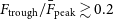 $F_{\mathrm{trough}}/ \bar{F}_{\mathrm{peak}} \gtrsim 0.2$
, indicating they may be potential LyC leakers.
$F_{\mathrm{trough}}/ \bar{F}_{\mathrm{peak}} \gtrsim 0.2$
, indicating they may be potential LyC leakers.

Following Hu et al. (Reference Hu2023), we classify the diagram (Figure 16) into three regions: (grey) minimal LyC leakage corresponding to systems with no or very few escape paths; (pink) significant leakage through ionisation-bounded channels with low column density (
 $f^{\mathrm{LyC}}_{\mathrm{esc}}$
 $\gt 10\%$
); and (blue) substantial leakage through large holes or density-bounded channels (
$\gt 10\%$
); and (blue) substantial leakage through large holes or density-bounded channels (
 $f^{\mathrm{LyC}}_{\mathrm{esc}}$
 $\gt 10\%$
). Based on this classification, we identify five LAEs as potential LyC leakers: four in the blue region (
$\gt 10\%$
). Based on this classification, we identify five LAEs as potential LyC leakers: four in the blue region (
 $A_{f} \lt 3$
), suggesting escape through density-bounded channels, and one in the pink region (
$A_{f} \lt 3$
), suggesting escape through density-bounded channels, and one in the pink region (
 $A_{f} \gt 3$
), indicating ionisation-bounded leakage in a multiphase medium. Using the empirical relation between peak separation and
$A_{f} \gt 3$
), indicating ionisation-bounded leakage in a multiphase medium. Using the empirical relation between peak separation and
 $f^{\mathrm{LyC}}_{\mathrm{esc}}$
from Izotov et al. (Reference Izotov2018), these five LAEs have
$f^{\mathrm{LyC}}_{\mathrm{esc}}$
from Izotov et al. (Reference Izotov2018), these five LAEs have
 $f^{\mathrm{LyC}}_{\mathrm{esc}}$
 $\sim 10$
–27%. Many LAEs reside in the grey region, suggesting lower LyC escape fractions compared to those five LAEs in the blue and pink zones. Additionally, as discussed in Section 5.2.5, an anticorrelation exists between the peak separation and
$\sim 10$
–27%. Many LAEs reside in the grey region, suggesting lower LyC escape fractions compared to those five LAEs in the blue and pink zones. Additionally, as discussed in Section 5.2.5, an anticorrelation exists between the peak separation and
 $F_{\mathrm{trough}}/ \bar{F}_{\mathrm{peak}}$
. Three LAEs in the blue zone exhibit higher net Ly
$F_{\mathrm{trough}}/ \bar{F}_{\mathrm{peak}}$
. Three LAEs in the blue zone exhibit higher net Ly
 $\alpha$
flux in the trough (i.e.
$\alpha$
flux in the trough (i.e.
 $F_{\mathrm{trough}}/\bar{F}_{\mathrm{peak}} \gt 0.2$
), supporting the conclusion that these galaxies have LyC-thin sightlines (Verhamme et al. Reference Verhamme, Orlitová, Schaerer and Hayes2015; Gazagnes et al. Reference Gazagnes, Chisholm, Schaerer, Verhamme and Izotov2020). Recent studies show that some high-redshift strong leakers instead exhibit large peak separations (
$F_{\mathrm{trough}}/\bar{F}_{\mathrm{peak}} \gt 0.2$
), supporting the conclusion that these galaxies have LyC-thin sightlines (Verhamme et al. Reference Verhamme, Orlitová, Schaerer and Hayes2015; Gazagnes et al. Reference Gazagnes, Chisholm, Schaerer, Verhamme and Izotov2020). Recent studies show that some high-redshift strong leakers instead exhibit large peak separations (
 $\Delta_{\mathrm{peak}} \gt 350\, \mathrm{km} \,\mathrm{s}^{-1}$
; Fletcher et al. Reference Fletcher2019; Naidu et al. Reference Naidu2022; Kerutt et al. Reference Kerutt2024). Hu et al. (Reference Hu2023) has established an empirical boundary between the blue and grey zones, located near a peak separation of 400 km s
$\Delta_{\mathrm{peak}} \gt 350\, \mathrm{km} \,\mathrm{s}^{-1}$
; Fletcher et al. Reference Fletcher2019; Naidu et al. Reference Naidu2022; Kerutt et al. Reference Kerutt2024). Hu et al. (Reference Hu2023) has established an empirical boundary between the blue and grey zones, located near a peak separation of 400 km s
 $^{-1}$
. Applying this boundary, along with the trough flux criterion of
$^{-1}$
. Applying this boundary, along with the trough flux criterion of
 $F_{\mathrm{trough}}/\bar{F}_{\mathrm{peak}} \gt 0.2$
, we identify an additional two LAEs, resulting in a total of five LAEs as possible LyC leakers.
$F_{\mathrm{trough}}/\bar{F}_{\mathrm{peak}} \gt 0.2$
, we identify an additional two LAEs, resulting in a total of five LAEs as possible LyC leakers.
Cosmological hydrodynamic simulations highlight that the central escape fraction (fraction of the flux near the systemic velocity or absorption trough) is a more robust diagnostic of LyC leakage, whereas peak separation or asymmetry separately are insufficient indicators (Choustikov et al. Reference Choustikov2024). Given the diagnostic potential of double-peaked Ly
 $\alpha$
profiles in constraining CGM kinematics, column density, and LyC escape, expanding double-peaked sample will provide a more statistically significant dataset to further explore the physical mechanisms driving Ly
$\alpha$
profiles in constraining CGM kinematics, column density, and LyC escape, expanding double-peaked sample will provide a more statistically significant dataset to further explore the physical mechanisms driving Ly
 $\alpha$
and LyC radiative transfer.
$\alpha$
and LyC radiative transfer.
6.5. Caveats in modeling and analysis
Finally, we note several caveats, particularly concerning the modeling of Ly
 $\alpha$
profiles and the interpretation of the derived results. Our analysis employs a spherically symmetric radiative transfer model applied to annularly averaged spectra, assuming that all Ly
$\alpha$
profiles and the interpretation of the derived results. Our analysis employs a spherically symmetric radiative transfer model applied to annularly averaged spectra, assuming that all Ly
 $\alpha$
photons originate at the galaxy center and then scatter through an expanding or infalling shell before escaping into the CGM. This geometry is highly simplified, and the assumptions of central photon production and spherical symmetry are not fully consistent with the setup of annular averaging. In addition, the best-fit models are mainly driven by the high-S/N spectra from the innermost bins, while the outermost bins, though critical for tracing gradients in spectroscopic properties, provide weaker constraints on model parameters. Extracting physical insights from different halo regions will require more realistic anisotropic radiative transfer models with non-uniform H i distributions. Thus, the results presented here should be regarded as average parameters representative of the modeled regions rather than as precise local measurements.
$\alpha$
photons originate at the galaxy center and then scatter through an expanding or infalling shell before escaping into the CGM. This geometry is highly simplified, and the assumptions of central photon production and spherical symmetry are not fully consistent with the setup of annular averaging. In addition, the best-fit models are mainly driven by the high-S/N spectra from the innermost bins, while the outermost bins, though critical for tracing gradients in spectroscopic properties, provide weaker constraints on model parameters. Extracting physical insights from different halo regions will require more realistic anisotropic radiative transfer models with non-uniform H i distributions. Thus, the results presented here should be regarded as average parameters representative of the modeled regions rather than as precise local measurements.
7. Summary and conclusions
We present a comprehensive spectroscopic study of 108 double-peaked LAEs in the first 35 fields of the MAGPI survey, including spatially resolved analysis of ten extended Ly
 $\alpha$
halos. To interpret the observed features in the context of gas kinematics in galaxies, we conduct radiative transfer modeling on both global and spatially resolved spectra. Our main findings are summarised as follows:
$\alpha$
halos. To interpret the observed features in the context of gas kinematics in galaxies, we conduct radiative transfer modeling on both global and spatially resolved spectra. Our main findings are summarised as follows:
-
• We apply an automated peak identification technique followed by spatial verification of double- and triple-peaked profiles, identifying 108 double-peaked LAEs. The number of double-peaked LAEs peaks at
$z = 3.2$
and drops sharply beyond
$z \gt 4$
, likely due to IGM attenuation. The double-peaked fraction at
$z \lt 4$
is
$\sim$
37%, consistent with previous such MUSE results at similar redshifts. Systemic redshifts are determined for 14 LAEs using C iii] emission. -
• We employ a forward modeling approach in which the intrinsic double-asymmetric Gaussian profile is convolved with the instrumental LSF to account for instrumental broadening. This allows us to recover the intrinsic spectra prior to broadening.
-
• We find that 17% of the double-peaked LAEs are blue-dominated, which may indicate gas accretion, although backscattering remains a possible alternative for sources without systemic redshifts. The blue-to-total flux ratio strongly depends on the Ly
$\alpha$
integrated total S/N. We observe an anti-correlation between Ly
$\alpha$
luminosity and the blue-to-total flux ratio, with fainter LAEs showing a higher fraction of flux in the blue peak. However, the relation flattens at lower luminosities and higher flux ratios. -
• The spectroscopic properties evolve with redshift: the red peak narrows significantly at
$z \gt 4$
, while the blue peak shows a weaker trend. Since the blue peak escape is strongly regulated by the IGM, its persistence implies that the red peak narrowing is instead driven by intrinsic galaxy/CGM evolution (e.g. reduced outflow velocity dispersion, lower H i column densities, or more ionised outflows). We therefore conclude that the H i column density in the ISM and/or CGM is the dominant factor shaping the Ly
$\alpha$
red peak, independent of outflow geometry or kinematics. -
• Several LAEs in our sample show residual trough flux between the two Ly
$\alpha$
peaks. The normalised trough flux density anticorrelates with the peak separation, both tracing H i column density. The trough flux also correlates with the blue-to-total flux ratio, a trend largely driven by the total line S/N. -
• We analyse spatially averaged Ly
$\alpha$
profiles across galactic radii in ten LAEs with extended Ly
$\alpha$
halos. Most of them show increasing blue-to-total flux ratios, normalized trough flux densities, and decreasing peak separations with radius. However, these trends are not always spherically symmetric – some systems exhibit significant azimuthal variations, with localised blue flux enhancements and reduced peak separations, complicating interpretations based on radial averages. Spatially-resolved radiative transfer modeling shows a clear line-of-sight effect: a declining shell expansion velocity and H i column density from center to outskirts, explaining the observed trends in blue-to-total flux ratio, peak separation and trough flux densities. One outlier shows increasing shell velocity and decreasing flux ratio in the outer halo. Though red-dominated, its kinematics resemble blue-dominated systems, suggesting a complex structure with central accretion and peripheral outflows. -
• We observe an inverse correlation between peak separation and red peak asymmetry. Highly asymmetric red peaks are found to exhibit smaller peak separations. Using peak separation, red peak asymmetry, and normalised trough flux, we identify 5 LAEs in our sample as strong LyC leaker candidates.


In general, we find that double-peaked Ly
 $\alpha$
profiles, both globally and locally, consistently trace the kinematics and distribution of neutral hydrogen. This demonstrates the power of such profiles in probing the gas dynamics and ionising photon escape in high-redshift galaxies. In the future, a more robust statistical analysis of the double-peak fraction and its redshift evolution will help to further quantify these trends. Additionally, advanced radiative transfer modeling that relaxes the assumption of azimuthal symmetry could provide deeper insight into the complex interplay between double-peaked profiles, gas kinematics, and escape of ionising photons in realistic, anisotropic environments in extended Ly
$\alpha$
profiles, both globally and locally, consistently trace the kinematics and distribution of neutral hydrogen. This demonstrates the power of such profiles in probing the gas dynamics and ionising photon escape in high-redshift galaxies. In the future, a more robust statistical analysis of the double-peak fraction and its redshift evolution will help to further quantify these trends. Additionally, advanced radiative transfer modeling that relaxes the assumption of azimuthal symmetry could provide deeper insight into the complex interplay between double-peaked profiles, gas kinematics, and escape of ionising photons in realistic, anisotropic environments in extended Ly
 $\alpha$
halos.
$\alpha$
halos.
Acknowledgements
We thank the anonymous referee for their constructive and insightful feedback, which significantly improved this paper. We thank the ESO staff, and in particular the staff at Paranal Observatory, for carrying out the MAGPI observations. MAGPI targets were selected from GAMA. GAMA is a joint European-Australasian project based around a spectroscopic campaign using the Anglo-Australian Telescope. GAMA was funded by the STFC (UK), the ARC (Australia), the AAO, and the participating institutions. GAMA photometry is based on observations made with ESO Telescopes at the La Silla Paranal Observatory under programme ID 179.A-2004, ID 177.A-3016. The MAGPI team acknowledge support from the Australian Research Council Centre of Excellence for All Sky Astrophysics in 3 Dimensions (ASTRO 3D), through project number CE170100013. K.G. and T.N. acknowledge support from Australian Research Council Laureate Fellowship FL180100060. SGL acknowledges the financial support from the MICIU with funding from the European Union NextGenerationEU and Generalitat Valenciana in the call Programa de Planes Complementarios de I+D+i (PRTR 2022) Project (VAL-JPAS), reference ASFAE/2022/025. This work is part of the research Project PID2023-149420NB-I00 funded by MI- CIU/AEI/10.13039/501100011033 and by ERDF/EU. This work is also supported by the project of excellence PROMETEO CIPROM/2023/21 of the Conselleria de Educación, Cultura, Universidades y Empleo (Generalitat Valenciana). CF is the recipient of an Australian Research Council Future Fellowship (project number FT210100168) funded by the Australian Government. CL, JTM and CF are the recipients of funding from the Australian Research Council (ARC) Discovery Project DP210101945. KH acknowledges support by the Royal Society through a Dorothy Hodgkin Fellowship to KA Oman (DHF/R1/231105). SB acknowledges the support from the Physics Foundation through the Messel Research Fellowship. SMS acknowledges funding from the Australian Research Council (DE220100003). LMV acknowledges support by the German Academic Scholarship Foundation (Studienstiftung des deutschen Volkes) and the Marianne-Plehn-Program of the Elite Network of Bavaria.
Data availability statement
All MUSE data used in this work are publicly accessible through the ESO archive (http://archive.eso.org/cms.html). Data products such as fully reduced data cubes and emission line fits will be made available as part of an upcoming MAGPI team data release (Mendel et al. in preparation; Battisti et al. in preparation).
Appendix A
Double-asymmetric Gaussian (DAG) fitting to each line profiles as discussed in Section 4. The original spectra are shown in black, while the best-fit convolved models are presented in green. The corresponding MAGPI IDs are shown in the top right corner, and the redshifts are displayed in the top left corner of each frame. For LAEs with a known systemic redshift, the redshifts are highlighted in magenta. The frames are arranged in ascending order of redshift.

Same as Figure A1.

Spatially resolved properties of extended Ly
 $\alpha$
halos in our sample. 1st panel: Ly
$\alpha$
halos in our sample. 1st panel: Ly
 $\alpha$
pseudo narrow-band image; Coordinates are centred on the brightest pixel. Shown contours represent 2 and 4
$\alpha$
pseudo narrow-band image; Coordinates are centred on the brightest pixel. Shown contours represent 2 and 4
 $\sigma$
significance levels. The black circles denote the location of stellar continuum detected in the MUSE white light image. 2nd panel: Spectra from annular bins as described in Section 5.3. Corresponding MAGPI IDs are shown in the top left corner. 3rd panel: blue-to-total flux ratio (
$\sigma$
significance levels. The black circles denote the location of stellar continuum detected in the MUSE white light image. 2nd panel: Spectra from annular bins as described in Section 5.3. Corresponding MAGPI IDs are shown in the top left corner. 3rd panel: blue-to-total flux ratio (
 $F_{\mathrm{blue}}\, / F_{\mathrm{total}}$
) map. 4th panel: Peak separation map.
$F_{\mathrm{blue}}\, / F_{\mathrm{total}}$
) map. 4th panel: Peak separation map.

Same as Figure A3.

Spectroscopic properties of 110 MAGPI double-peaked LAEs in the sample, in order of increasing redshift.


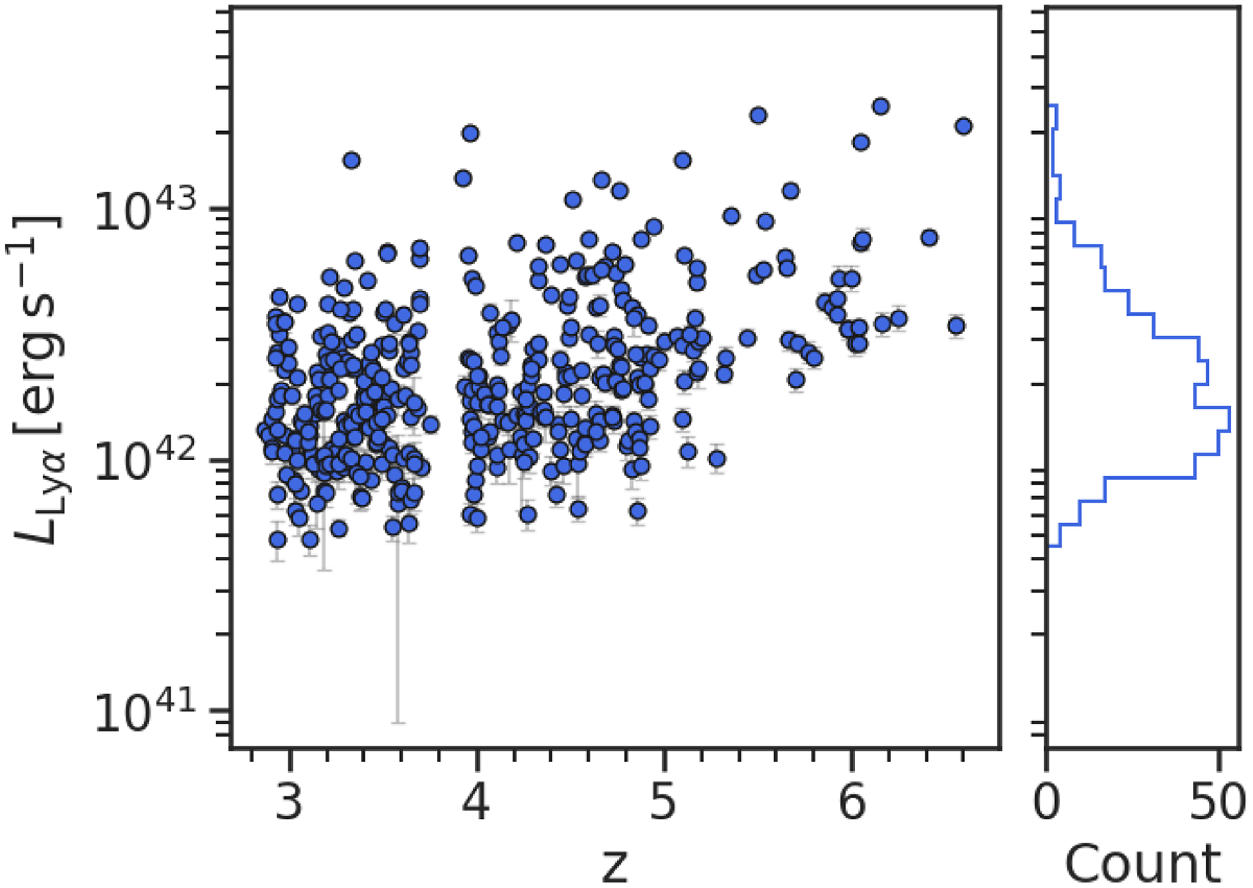


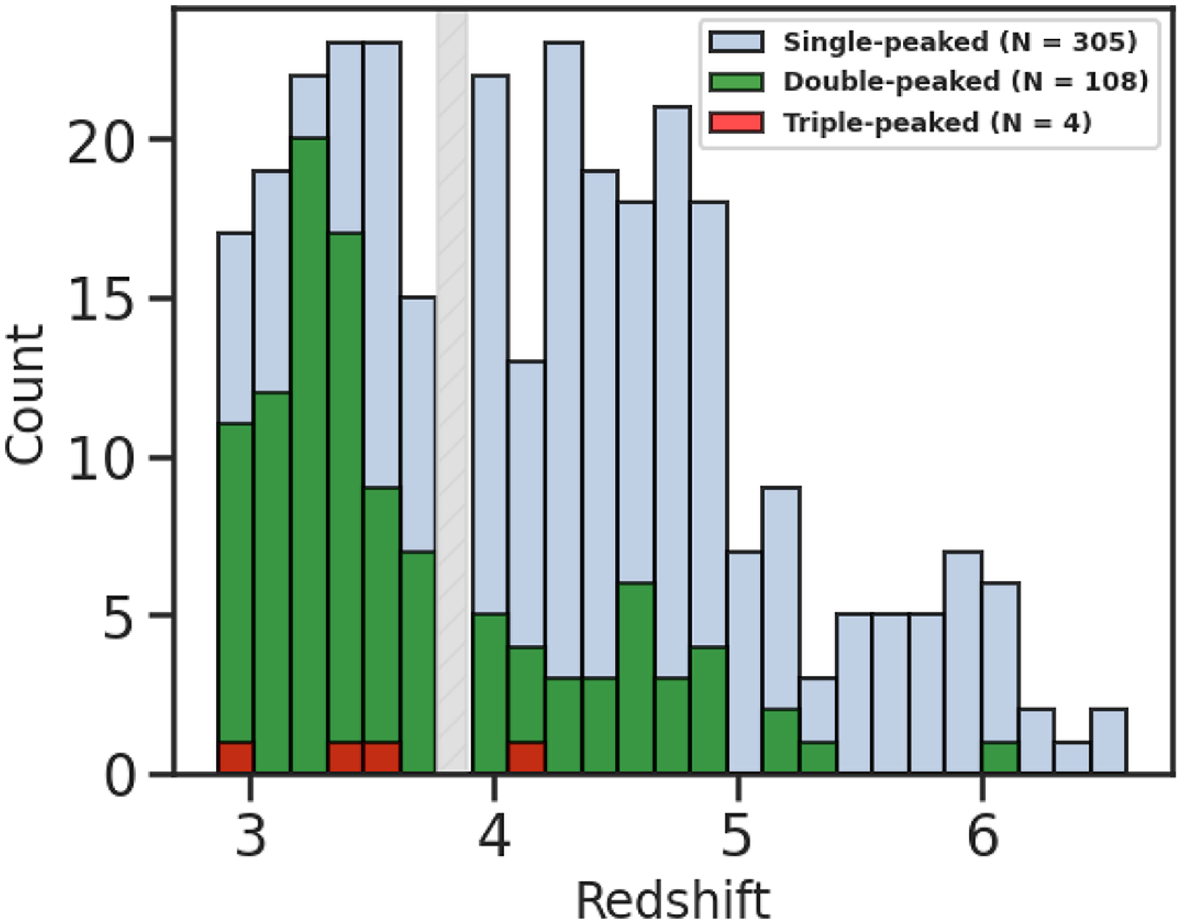


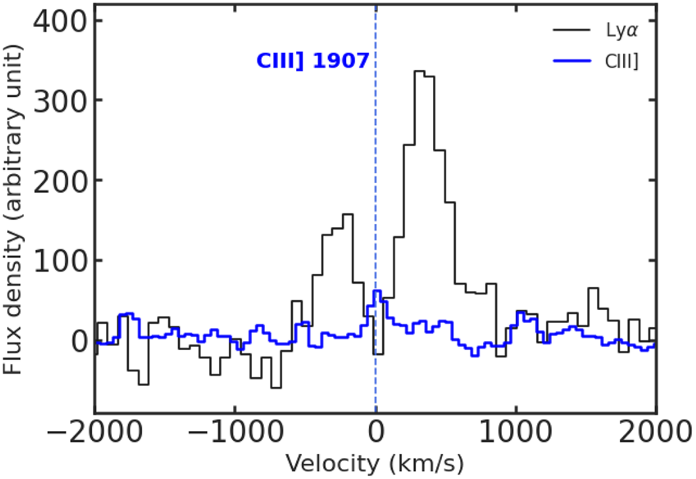


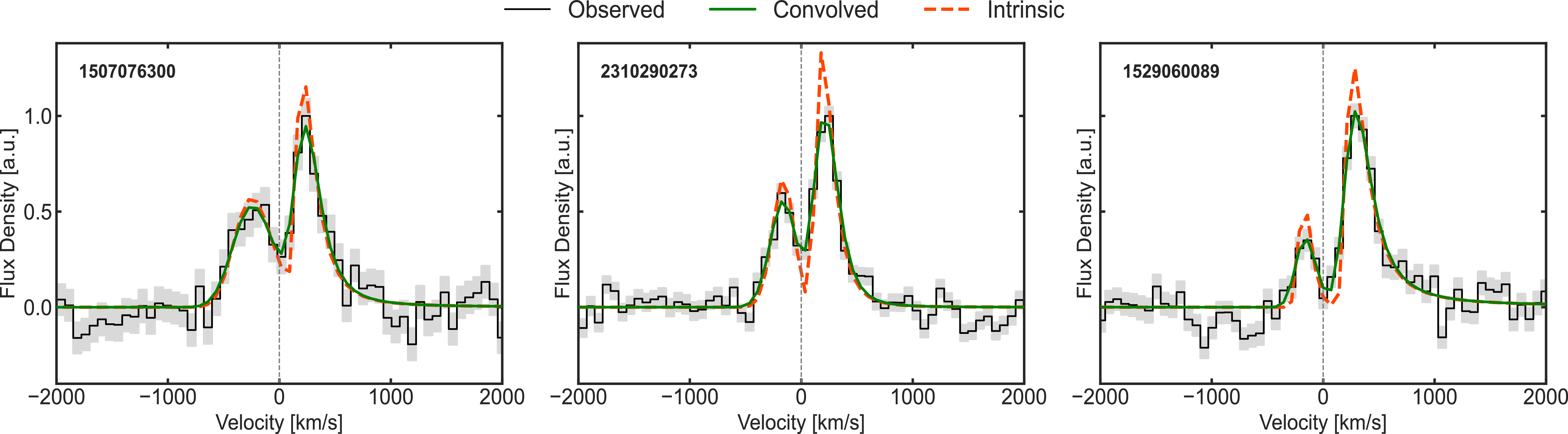

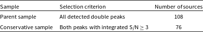
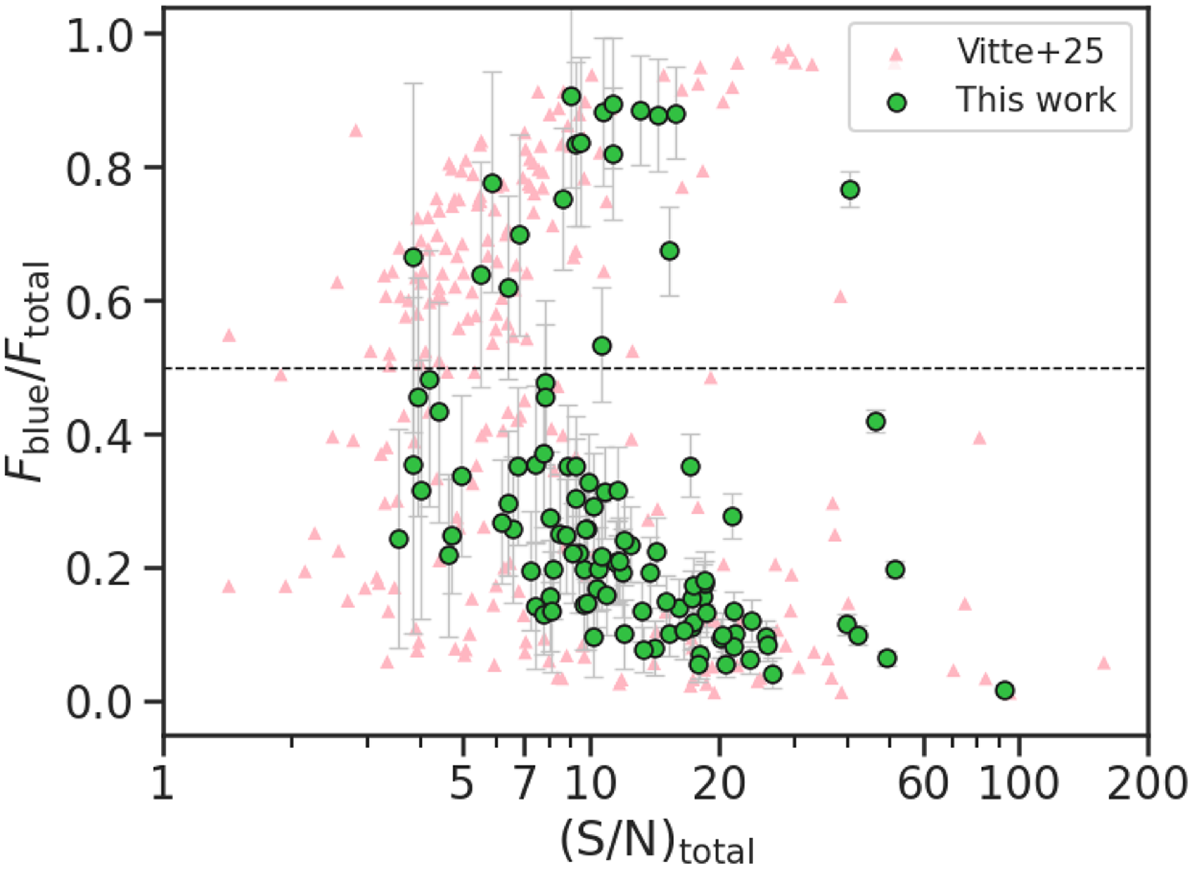

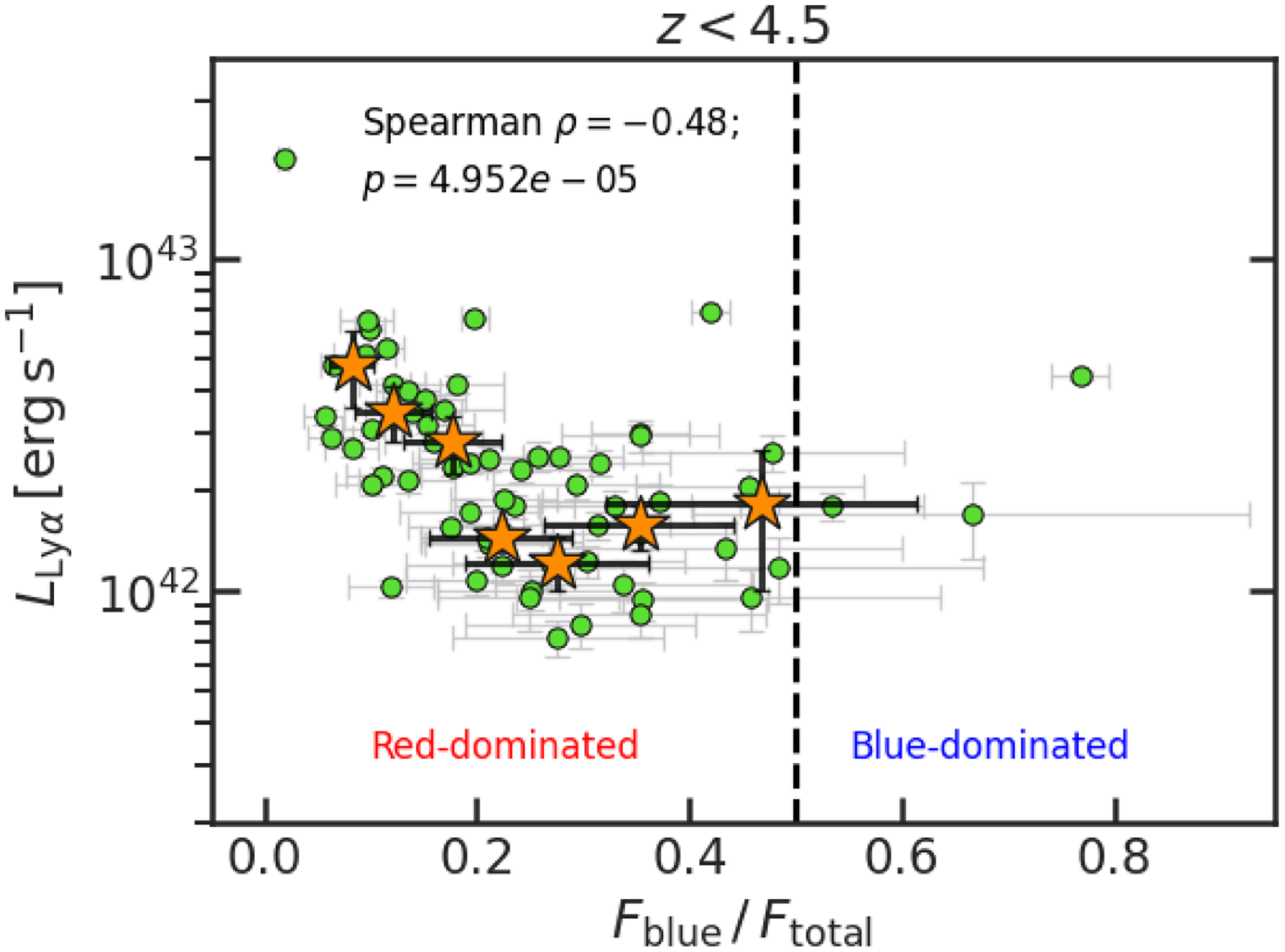


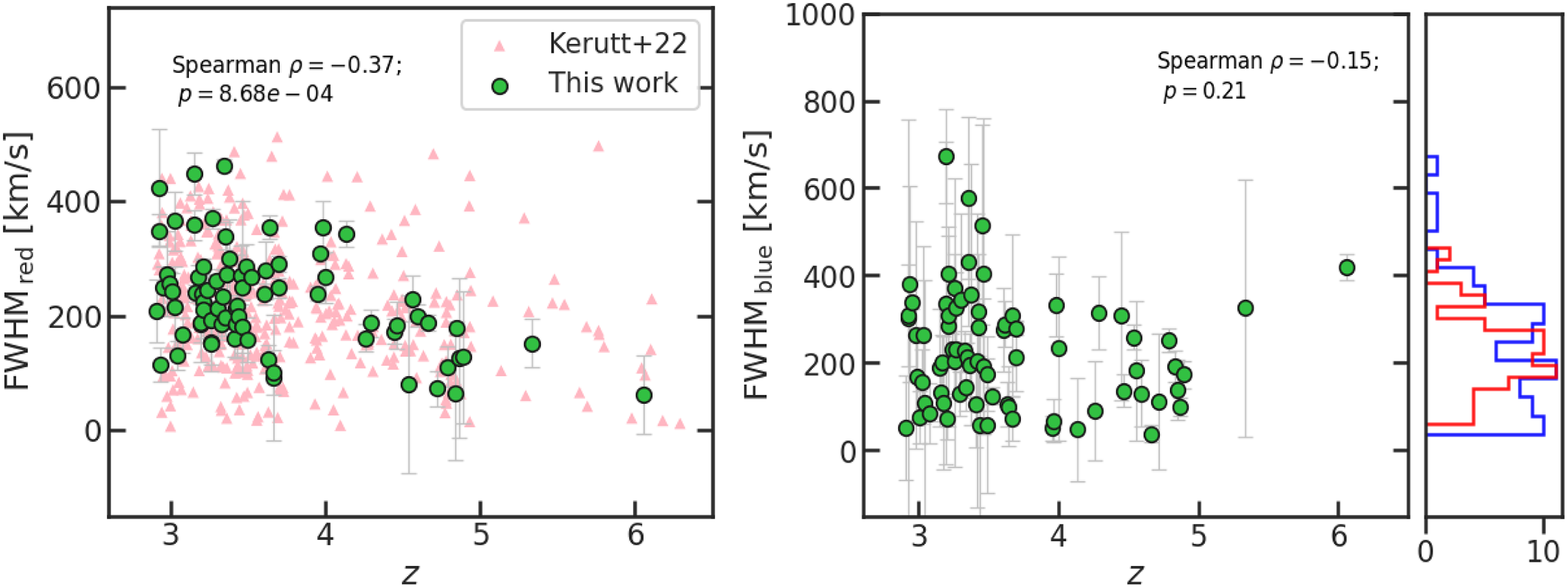


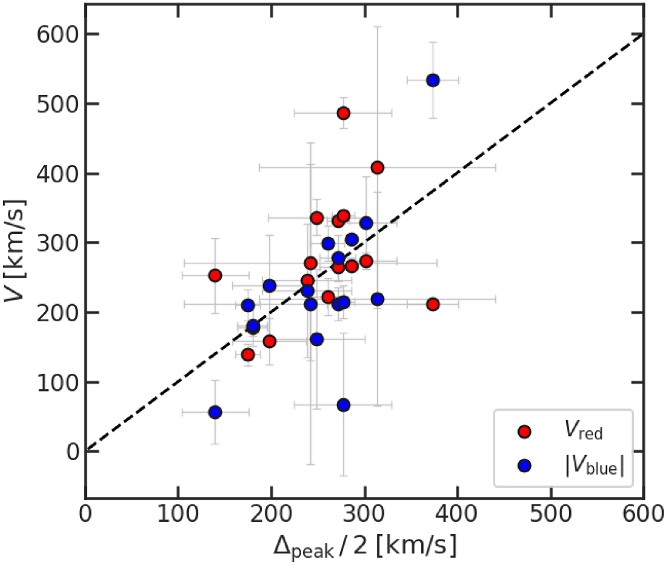


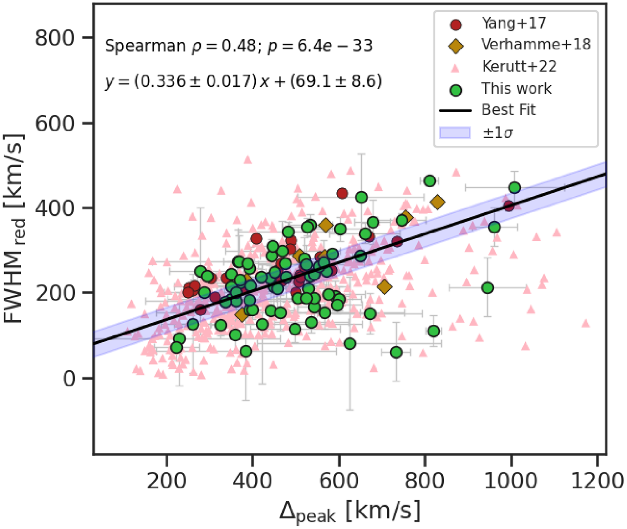


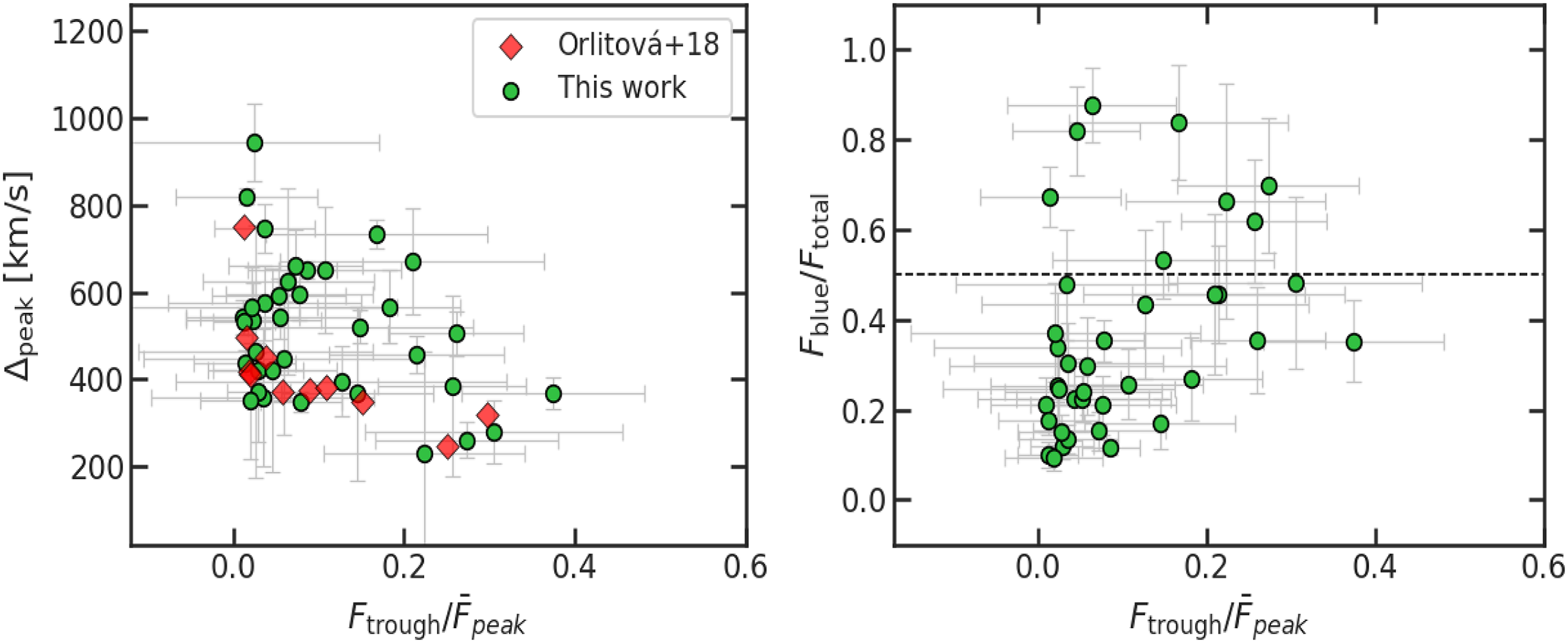


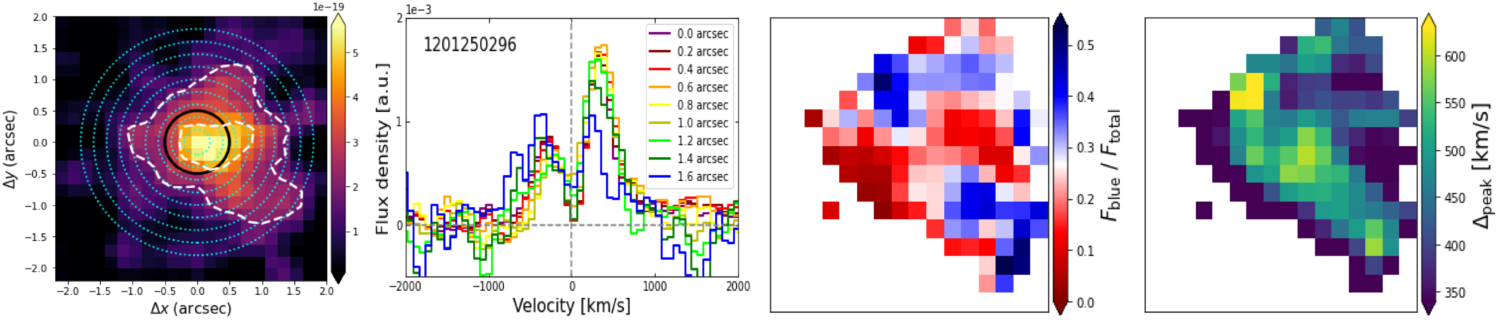


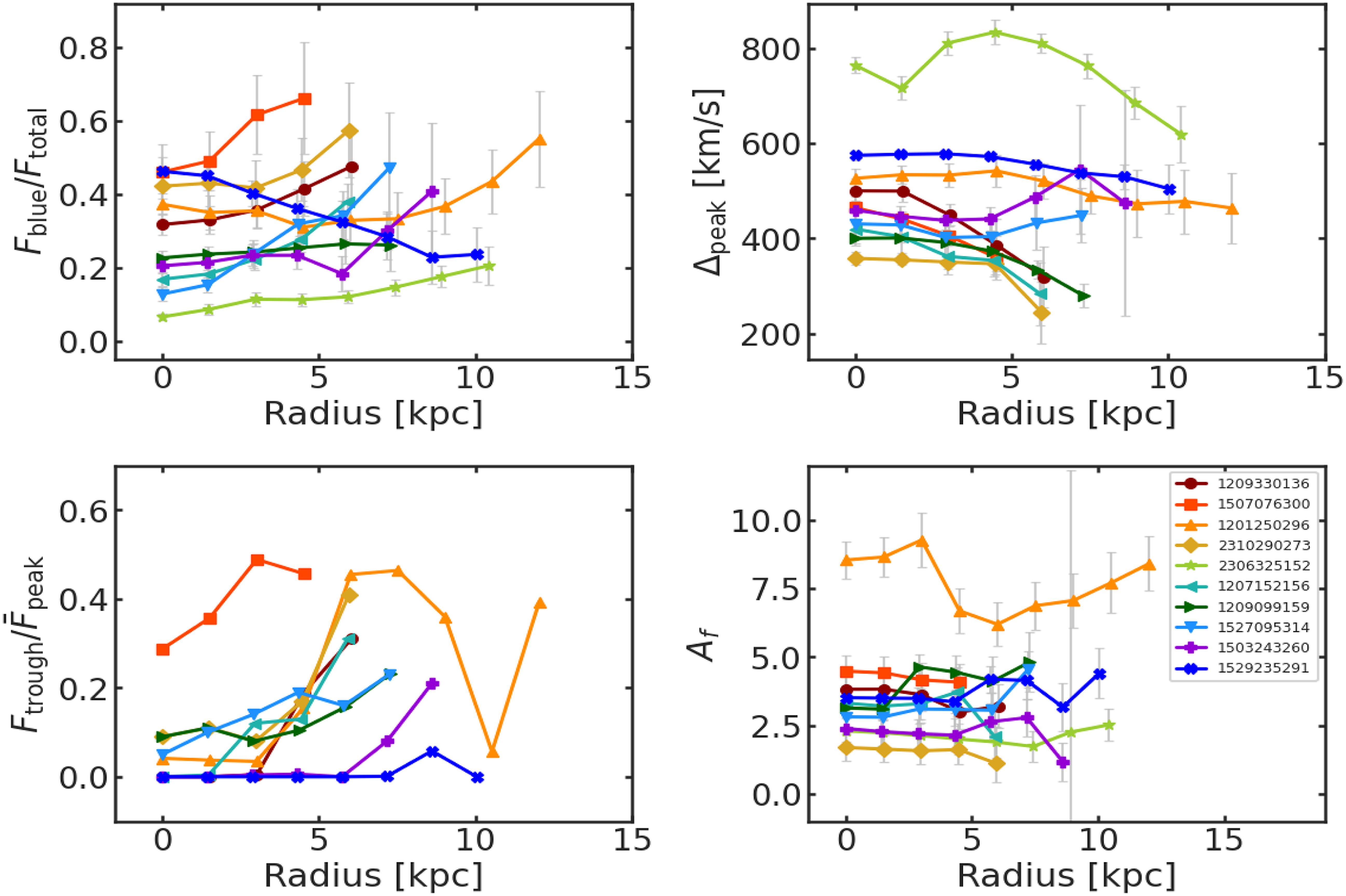


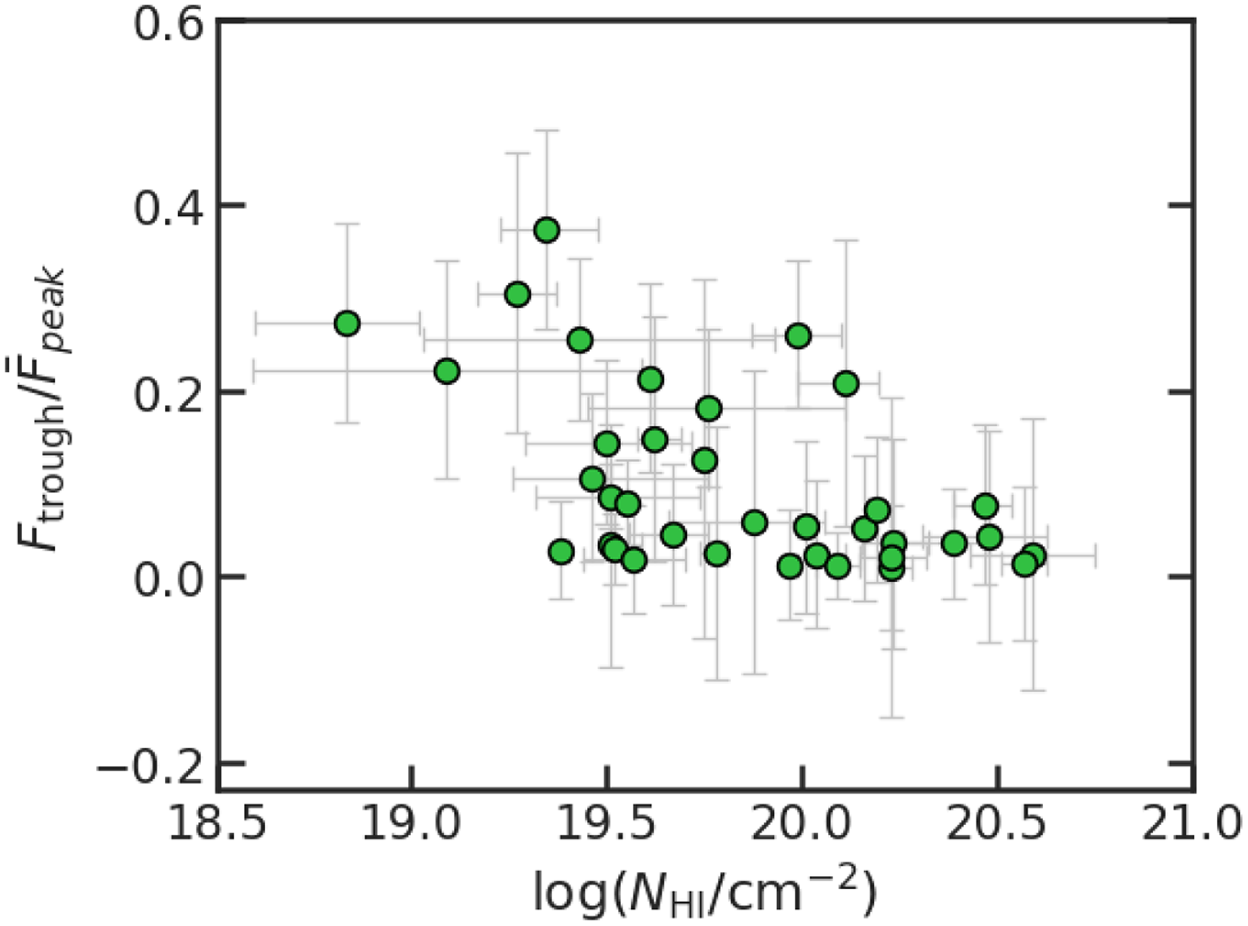


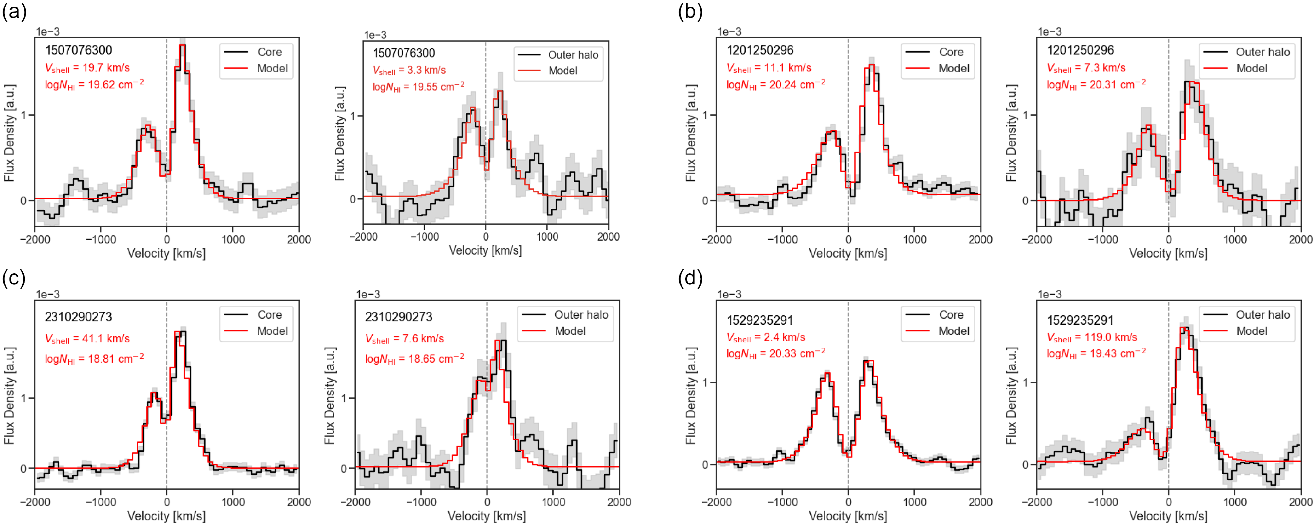

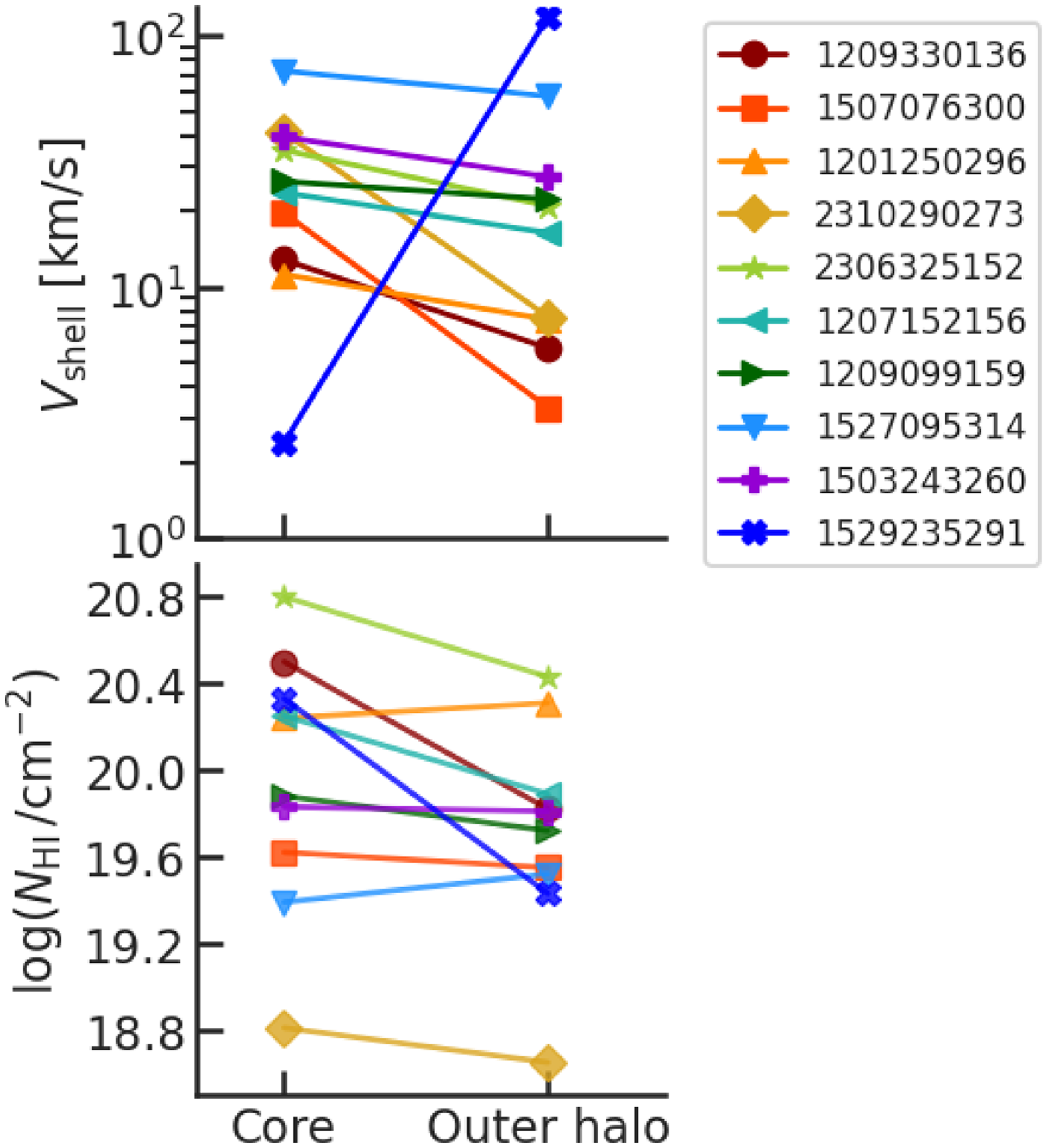

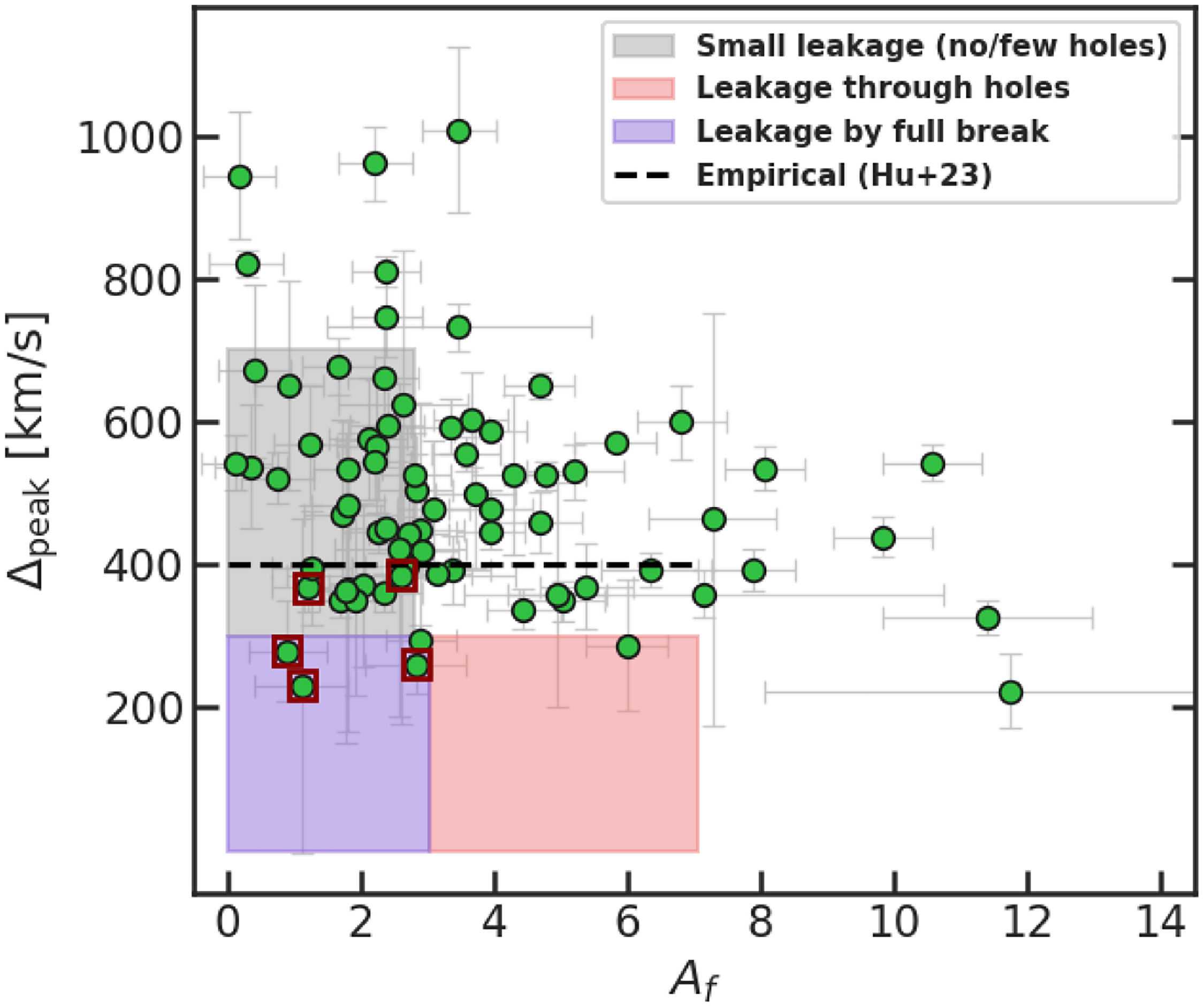


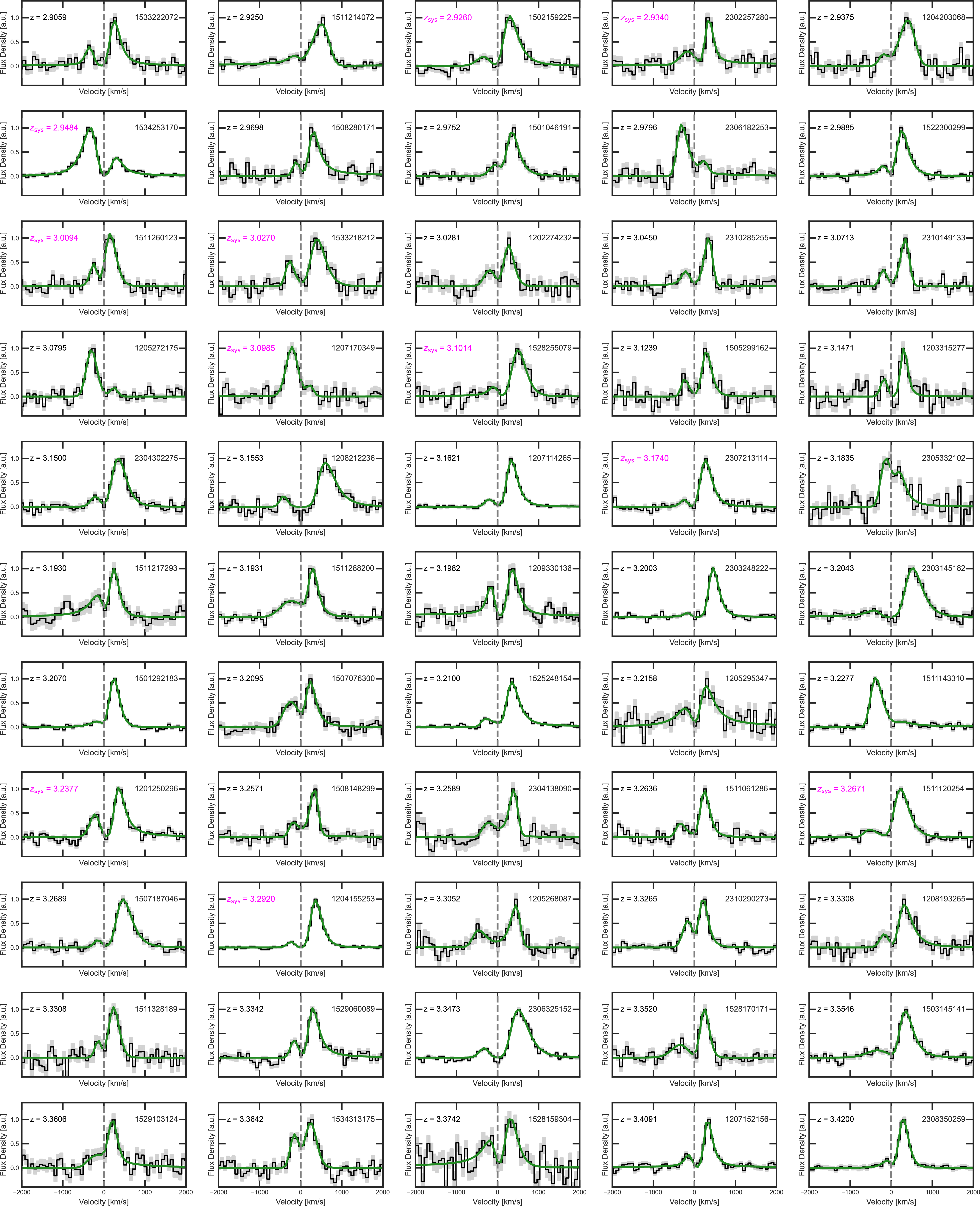
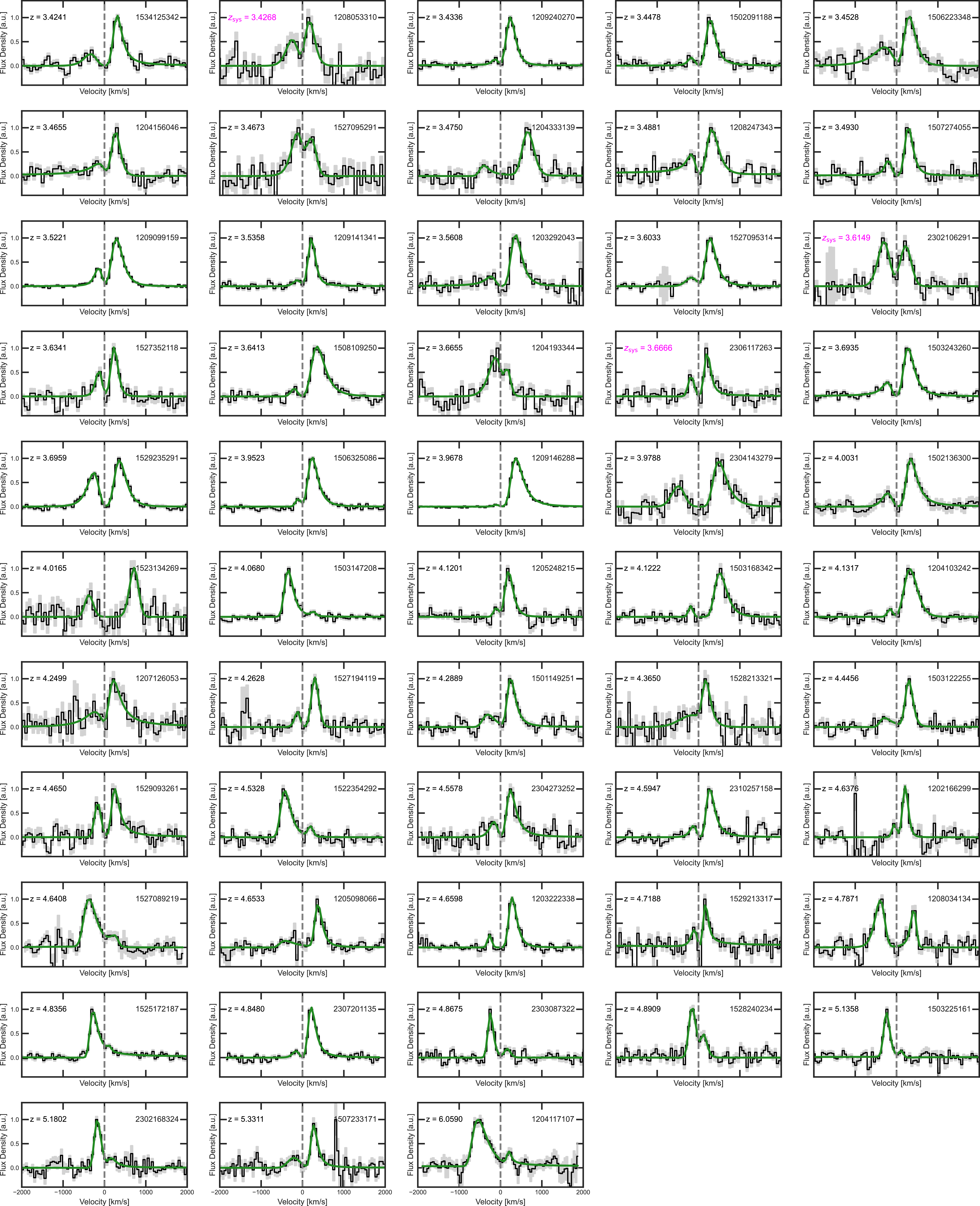
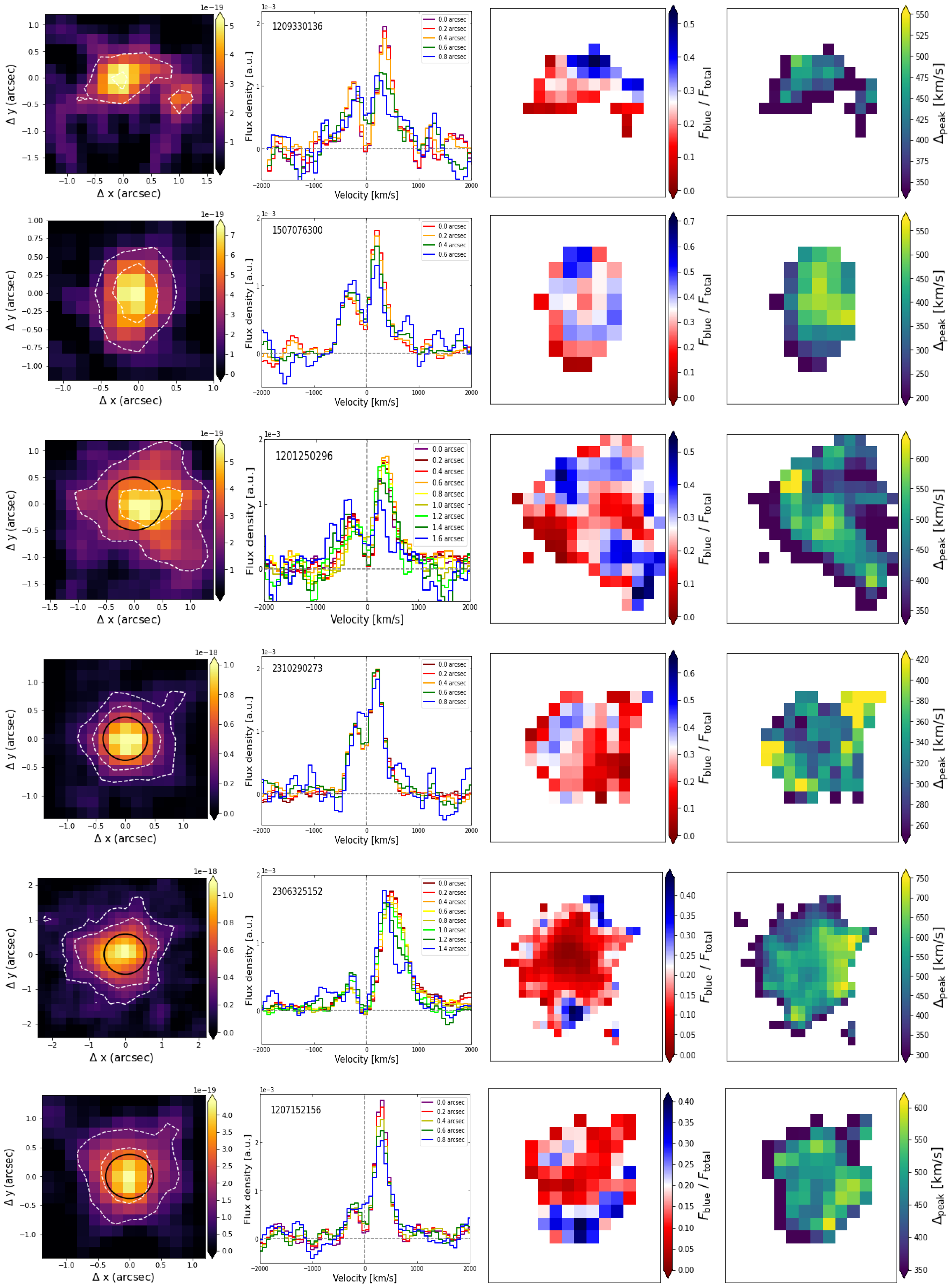


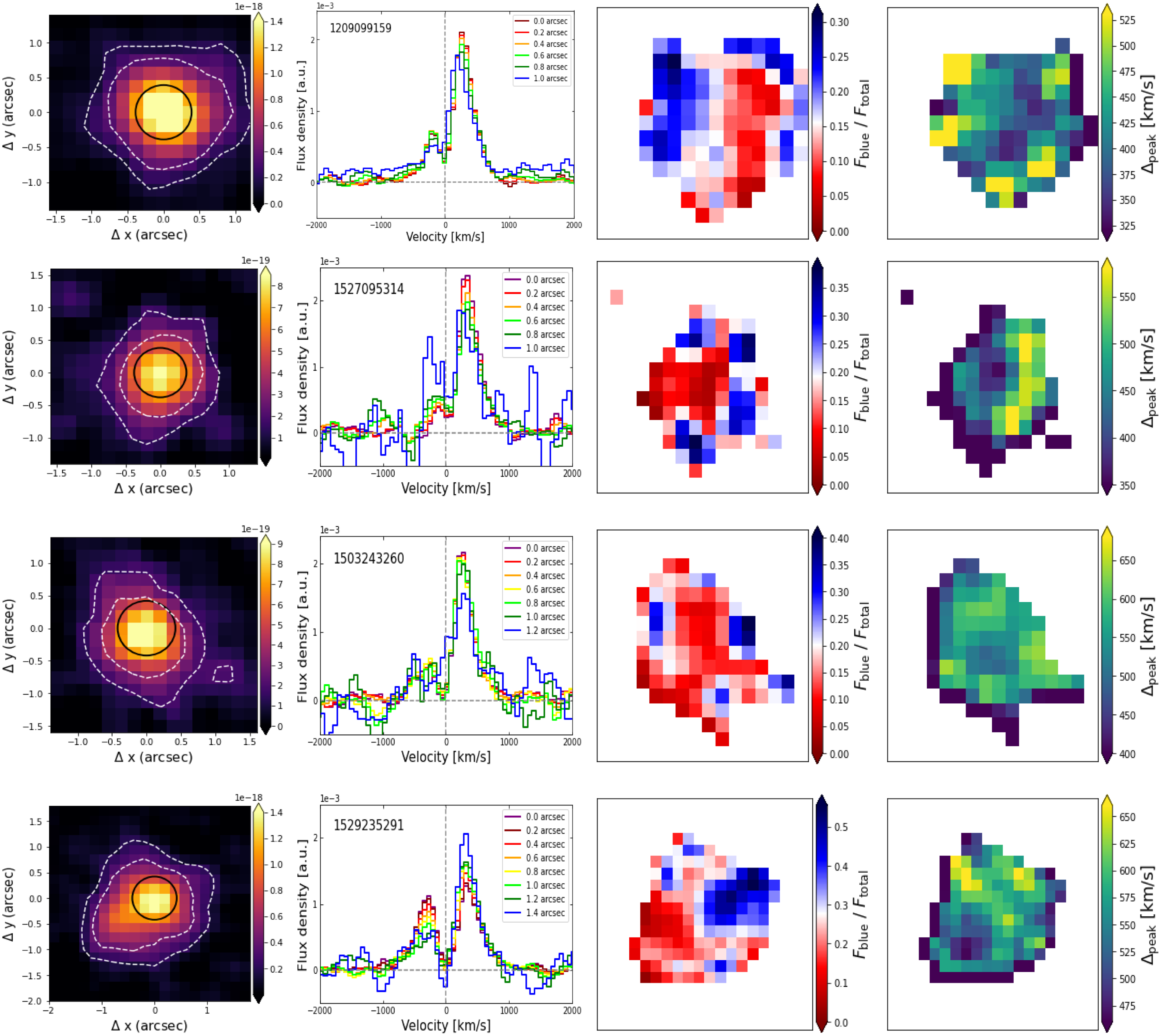
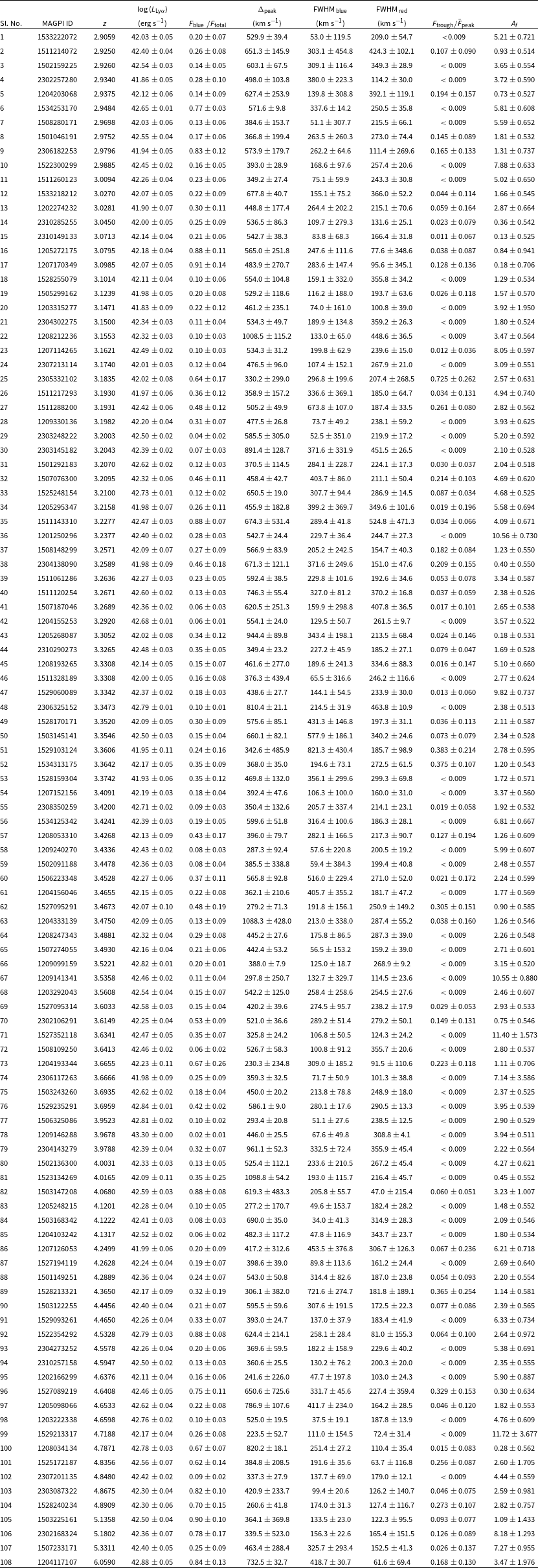

 Open access