This discussion relates to the IFoA sessional webinar presented by Matt Fletcher and Piero Cocevar on Wednesday, 10 September 2025.

Moderator (Dr C. N. Reynolds, F.I.A., C.Act): Welcome to today’s webinar on “Graduating Mortality Base Tables,” which is jointly produced by the IFoA’s Mortality Research Committee and the CMI. I am Chris Reynolds, and I will be the Chair for today’s session. I am also involved in the CMI, as Chair of the CMI Assurances Committee.

Today’s webinar is part one of a two-part series focused on graduating mortality base tables. I am pleased to be joined by Matt Fletcher and Piero Cocevar. Matt (Fletcher) is an actuary with 25 years of consultancy experience. He is the head of Aon’s Demographic Horizons team, where he provides advice on setting best estimates and evaluating risk for longevity. He does this both for the UK and overseas. Matt (Fletcher) has held many specialist longevity positions in the UK actuarial profession, including being a founder member of the COVID-19 Actuaries Response Group. He is a former Chair of the CMI Self-administered Pension Schemes Committee, and he is the current Chair of the IFoA’s Mortality Research Steering Committee.

Piero (Cocevar) is an actuary with 30 years of experience in the life insurance industry. He is the Head of Insurance, Strategic and Operational Risk at the Phoenix Group. He is also a longstanding volunteer with the CMI where he has contributed to work on both the Annuity Committee and the Mortality Projections Committee. Piero (Cocevar) is here today representing himself as a member of the CMI Annuities Committee.

Mr M. K. Fletcher, F.I.A., C.Act: This is a webinar in two parts. Across the whole of the two parts, our aim is to give an idea of how mortality tables are produced via graduation of mortality rates. We will also touch on morbidity as the CMI also produces critical illness and income protection tables. My experience and that of the other speakers, both today and next week, mainly relates to CMI graduations. Our examples will mainly be based on CMI tables, but the theory and practice will translate into other applications and areas.

This first session focuses on the theory of graduation. The session next week looks more at the practical aspects. Taken as a whole, our aim is to help you understand the data that are needed to carry out graduations, the pros and cons of graduating mortality and morbidity, the principles of graduation techniques and how to apply these in practice, and how to engage with your stakeholders. So, we cover the matters necessary to meet the requirements of stakeholders before, during, and after the production of mortality tables.

We start with a very brief history of mortality analysis, which started with the analysis of London death records by John Graunt in the 1660s. In 1693, Edmund Halley, after whom the comet is named, published what was arguably the world’s first life table, setting out the chances of survival to each age. After this, through the 19th and early 20th century, mortality curves were generally drawn by eye to provide a reasonable fit to the raw data that had been collected. Just over a hundred years ago, the CMI was established in the UK to collect and analyse data from insurers and, later, pension schemes. The CMI soon started producing graduated mortality tables that were based on numerical rather than graphical methods. By this point, the Gompertz and Makeham formulae were well known to actuaries, having been set out in the 1800s. The general Gompertz-Makeham approach started to be used by CMI in the mid to late part of the 20th century and is still in common use today. We will come back to this in Piero (Cocevar)’s section. Bringing things up to the present, about ten years ago the CMI set up a Graduation and Modelling Working Party, to which both Piero (Cocevar) and I both contributed. This had the aim of reviewing and assessing the theoretical and practical aspects of the graduation process. The Working Party ultimately produced a working paper and software for CMI subscribers. We will talk through some of the output and findings of this paper.

We are aware that we have an audience today who may have different levels of prior knowledge of mortality analysis. Thus, we wanted to define a few key terms that we use at various points through the presentation. Firstly, the concept of exposure to risk. In mortality analysis, we need to know how long someone was both alive and in the dataset. Once we have that for each individual, we can sum those up across a group of individuals to get an overall exposure across a different range of ages. If we also then know how many people die at age x in the same population, we can compare these actual deaths to the exposure to give a crude mortality rate for age x in the population. In mortality graduations, we often think in terms of the force of mortality. The force of mortality for μ_x for age x can be conceptualised as the probability that an individual aged x dies in the next infinitesimally small time period. We will see this concept come up later when we start looking at choosing our statistical model for deaths.

If we convert the force of mortality into a probability of death and sum across all individuals, this will give us the expected number of deaths at age x across our population. It is important that expected and actual deaths are calculated consistently; Piero (Cocevar) will expand on this later. The final point to mention is that the definitions here count each life equally. It is possible, and quite common and useful, to add different weights into the mix. For example, the CMI SAPS tables for pensioners have versions that are lives-weighted and amounts-weighted. This can be helpful when calculating a pension scheme’s liabilities, which are inherently weighted towards those with higher pensions.

The next step is mortality graduation. Even for a very large population, mortality and morbidity data does not follow a completely smooth pattern, even though we might have an expectation that the true underlying force of mortality, or force of morbidity, should be smooth both across time and by age. The charts on the right in Figure 1 show some examples of noisy data that CMI have obtained and graduated. The top right chart shows crude rates by age for female non-smokers from the assurances dataset, where you can see various bumps in the data between the ages of about 45 to 57. The bottom chart shows even more noisy data from the SAPS pension scheme dataset. We see this noisiness when we split a large population into socioeconomic groups. At its core, graduation is just the process of taking that noisy, observed mortality data and producing a smooth set of mortality or morbidity rates.

Figure 1. What is graduation?

Why do we graduate mortality rates rather than just using the raw rates? Typically, we see mortality rates being graduated for national populations, which is usually done by statistical bodies such as the Office for National Statistics in the UK. It gives us a smooth baseline set of mortality rates by age for the population instead of having to rely on raw data. Where we have subpopulations of suitable size, for example male annuitants or female pensioners with high pensions (over £16,000 per annum, say) we would likely want to graduate these tables for these subpopulations separately to allow us to recognise differences in mortality between subpopulations. This might simply be a different level of mortality, so higher or lower than an existing population, or it may be an observed difference in the shape of mortality. For example, it might be close to population-level mortality at some ages but further away at other ages. The table to the right of Figure 2 shows some life expectancies at age 65. These are period life expectancies, excluding allowance for future improvements. The top line is for the UK population and then the rest are the results of some selected CMI graduations. For males, there is about a three-year range in life expectancies across the different tables. For females it is around two years, which indicates that there is a difference in the levels of mortality in these subpopulations. It is part of the reason we graduate for these different populations. Using graduated tables rather than using raw mortality figures gives us a stable, reliable and smooth set of mortality rates. It also gives actuaries a common currency to work with. For example, every actuary working in insurance or pensions in the UK will be familiar with the SAPS S4 tables. Different parties can understand what is being referenced without having to share a full set of mortality rates each time. It also gives a good starting point against which to benchmark mortality experience in a subset of data, which is typically a smaller subset than the graduated set of data.

Figure 2. Why should we graduate mortality?

Having said why we would graduate mortality, there are some reasons why or where we would not want to produce graduations. Firstly, an obvious one is where there is insufficient volume or quality of data. You do need a lot of high-quality data on deaths and exposeds to risk to produce a credible graduation. In particular, it is important to have age-by-age data so that we can produce a graduation that is not biased by changes in the mix of ages in the population. Secondly, even if we do have enough data, it might be that perfectly suitable tables exist already. This is one reason, for example, why we do not produce mortality tables on an annual basis even though it would theoretically be possible to do so. The existing tables should still be suitable for almost all purposes. Thirdly, we should be wary that tables are not treated as being recommendations for use for a particular population. For example, if a male pensioners table is created, some users may view this as being a recommendation that this table should be used unadjusted wherever male pensioner liabilities are being calculated, even where this population being considered might have much heavier or much lighter mortality than a typical male pensioner population. It is fair to say this is partly a communication point. Users of the tables should be warned against this when the tables are published. It may be a reason to consider an alternative to graduation for particular subpopulations. Finally, it would be quite possible to use the existing CMI datasets. These are based on lots of insurance and pensioner data. We could produce huge numbers of graduations using all sorts of different ways of subdividing or combining data. In general, we seek to avoid complexity from having too many tables. We focus our graduation on key groups and we only comment on differences for others. To take a SAPS example, when we produced the S3 and S4 tables, we did some analysis of differences between public and private sector mortality experience, but we stopped short of producing additional graduations for the two sectors because we felt that would be overly complicated.

If we are not graduating mortality but we have looked at the mortality experience and we see that the population in which we are interested has a different mortality profile to our existing tables, we should not just ignore that. We should reflect it when coming up with a mortality assumption for that population. There are lots of different options to use when adjusting existing tables. We could simply use a flat scale. For example, use 110% of the rates in an existing table at all ages. This is very simple to describe and understand. The chart on the right in Figure 3 shows an example of what happens if you do a flat scaling, and it does significantly change the assumed mortality rates relative to the existing table at high ages. Those are ages where we are unlikely to have much data. You need to consider whether this is material to the results and whether it is a desirable feature of the assumption that you are using.

Figure 3. Alternatives to graduation.

An alternative might be to restructure the scaling applied. For example, using 90% up to age 60, tapering to 100% at age 90. This is obviously a more complex structure. It is slightly harder to implement and to communicate. Arguably, it might give a more appropriate shape, particularly at those higher ages. Without going into detail, there are lots of other ways to tweak mortality that stop short of carrying out full graduations.

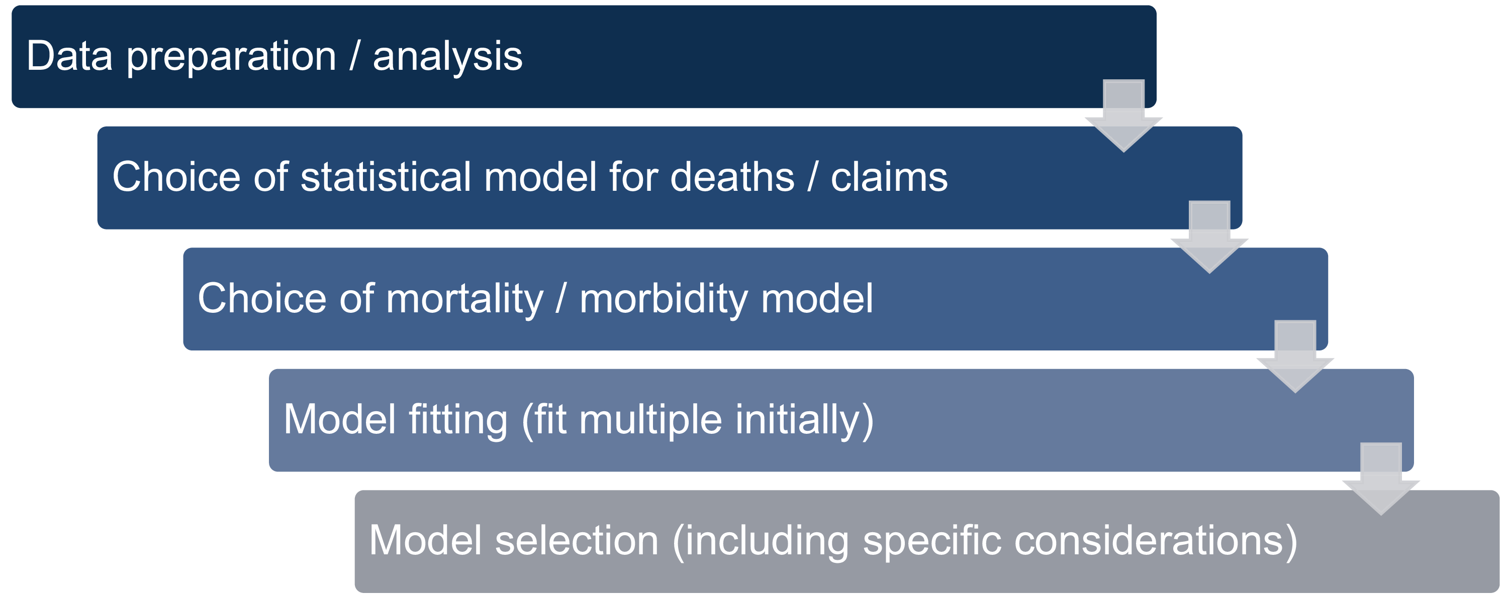
Once we have decided that we do want to graduate mortality for a dataset, we need to determine our objectives. Initially, it is worth saying that even though modern graduation involves a significant amount of statistical modelling and testing, there is still a lot of judgement to be applied throughout the process. When graduating we have several objectives. We want to produce a smooth set of tables and remove random fluctuations that may be present in the data. We want to remain close to the observed experiences but without over-fitting our model. We aim to produce a set of tables that are practically useable and fit for their purposes. Ideally the table of mortality rates should increase monotonically with age, and it should be continuous without jumps or gaps between different ages, even if different formulae are used for different age ranges.

Our process for graduation should follow the steps that are set out in Figure 4. I am going to cover data preparation, then I am going to hand over to Piero (Cocevar) to go through the various stages in the model selection and fitting process. When we are collecting our mortality data for graduation, our initial objective is to calculate crude mortality, or if we are doing morbidity analysis, crude morbidity rates by age. That is, deaths or claims divided by exposure. We collect data for individual lives. We collect deaths data for mortality or claims data for morbidity. We also collect details of dates when each life went on risk and off risk during the investigation period. This is hugely important to enable us to accurately calculate the exposure part of the formula. It is worth pointing out here that for CMI, typically we would get data from multiple sources. So we would get data from multiple insurers for insured data and from multiple consultancies and other sources like the Pension Protection Fund for pension data. It is quite possible for data for a graduation to come from a single source instead, either for a whole population or from a single organisation. It is important to validate the data – to make sure it is fit for purpose – before you start on the graduation. We could quite easily spend this whole talk going through the data validation processes but suffice to say it is vital for deaths and exposures to be consistent to enable us to do sensible graduations. When doing that, we need to make sure that we query abnormal data. Anything incorrect should be either corrected or excluded from our dataset. Then, when we have credible data for individual lives, we usually aggregate by age as that is the key rating factor for mortality.

Figure 4. Graduation process.

Once we have data by age, we can start to subdivide it into homogeneous subsets. These are subsets of the data that are large enough to justify separate graduations but where we would expect mortality or morbidity experience to be similar across that subset. This can be monitored before graduating by carrying out regular experience analyses for subgroups of interest and, again, typically those would be measured against existing tables. That should identify differences in mortality experience between different groups. The groups into which we might split data will depend on the availability of data fields. Various rating factors are used across the different CMI investigations as shown in the following examples. Sex is almost always used as a rating factor as mortality does differ significantly for males and females. Smoker status is a possible rating factor as there are differences in experience for smokers versus non-smokers. CMI do not have smoker status for pension schemes, but they do for some of the insured data. Socioeconomic measures are relevant. CMI have some data on deprivation across most of their datasets and we do see different experience depending on the level of deprivation in the area where an individual is living. Policy or pensioner type is potentially important. Examples of this include ill health retirements or contingent dependence and benefit or pension amount. Benefit or pension amounts are clearly correlated with deprivation but when looking at the SAPS and other data CMI did see benefit in using pension amount alongside deprivation when the SAPS data was split for graduation. The factors are not perfectly correlated so it makes sense to look at pension amount as well as socioeconomic factors.

When determining the subsets of data to analyse, we should consider how much data is in each subset. It is possible that low data volumes may mean you cannot realistically use exactly the subsets that you want. Subdividing in the way that you prefer may mean, for example, that you cannot graduate across the full range in which you are interested. An important decision is the time period of data to use. Using too long a period could mean that the early data might not be consistent with the later data, whereas too short a period may mean that you do not have enough data to perform graduations. For example, SAPS uses data for the full years 2014 to 2019, which is a six-year period.

Finally, it is important to consider what subsets are likely to be of interest to the ultimate users of the tables, because there is no point in producing tables that no one would ever use. Once you have decided on which subsets of data you are going to use, it is then time to start choosing and ultimately fitting your model.

Mr P. Cocevar, F.I.A., C.Act: In the next part of the presentation, we are going to cover the process of choosing a statistical model for our data, which will be the cornerstone for deciding on the actual mortality law to fit. Important considerations are how to select the models from the many models available and how to choose appropriate parameters. We mainly focus on the activity of the CMI committees and my own experience. Once you have the subset of data ready for graduation, you need to make an assumption about which statistical model to use. In terms of what the CMI usually does, the common assumption is that deaths are distributed with a Poisson distribution. This is simple and works well for large datasets. In the Poisson model the mean and the variance are both equal to the central exposure multiplied by the force of mortality or morbidity. The Poisson distribution arises quite naturally for independent events and a survival model. The model describes how your data is statistically governed. It helps you with the next steps when you want to fit your model. The Poisson model allows the use of maximum likelihood estimation, which is a simple statistical approach obeying parametric laws. Although the Poisson model is the model we use at the CMI, it is not the only model available. We recognise that there are alterative statistical models to use when the Poisson does not work well. Generally, with the CMI data, we have very large datasets, and the Poisson distribution works reasonably well. An additional reference about this can be found in Working Paper 77, which summarises the work of the Graduation Modelling Working Party.

Once we have a statistical model, we can move on to choosing a mathematical formula to fit mortality or morbidity rates. The early historical approach, as outlined previously, was for people to draw a curve. Now we have computers and a rich family of models from which we can choose. Many formulae will work and provide a visually good fit. Choosing the formula is where theory meets actuarial judgements. It is not just about fitting the data well. There are other considerations. We will link back to the graduation objectives. The formula we choose needs to achieve an appropriate balance. You should choose a formula that balances what I call biological realism, good statistical fit, and actuarial usability. By biological realism I mean a relationship with the survival of humans. As I said, there is not a single law that is the best. The right choice depends on the data you have and your ultimate purpose.

We will now focus on the parametric formulae that the CMI uses. We start with the Gompertz law. In 1825 Gompertz observed that adult mortality increases roughly exponentially with age. Another way to look at this is that the logarithm of deaths is linear. That is really the fundamental basis of the Gompertz-Makeham model. Makeham observed that you can get a better fit to the younger ages if a non-exponential element is added to the formula. The CMI has taken this concept and allowed higher-order polynomials in age and generalised this concept in the third formula in Figure 5. You can choose the order of the polynomial used in the exponential and non-exponential terms. Much of the work the CMI committee does is around choosing the right order of the polynomials. There are other, more complex laws that could be used. For example, the Heligman-Pollard law has eight parameters. These complex laws can fit any pattern very well but at the cost of simplicity.

Figure 5. Choice of mortality/morbidity model I.

Figure 6 highlights that, in practice, the CMI committees have tended to use the simple Gompertz model, or the Gompertz-Makeham model, with the exception of the income protection committees that used GLMs. As you can see from the table in Figure 6, simpler laws with fewer parameters are often required for the mortality graduation at older ages for SAPS or annuities. On assurances, you can see there is the use of a Gompertz-Makeham model at younger ages where the exponential law does not work as well. The choice of model is driven by balancing several factors. Simplicity is desirable as you do not want to have a complex, difficult to explain model. It is important to consider how well the model fits the data. There is a wider point about consistency with similar datasets where graduations have been already performed.

Figure 6. Choice of mortality/morbidity model II.

Once you have obtained your dataset and chosen your statistical model and your law of mortality, you must then fit the coefficients. The Maximum Likelihood Estimation process finds the set of model parameters that make sure the observed deaths count is the most probable under the Poisson distribution by giving the right weighting to each age in proportion to exposure. The important thing is to have good and well-tested software. CMI committees have generally used the CMI graduation software that was initially developed by the Graduation Modelling Working Party. There have subsequently been a couple of additional versions of that software. It is reliable and well-tested and not only fits the Gompertz-Makeham formula but also other formulae.

We select our model parameters using an iterative process. We start with the simplest mortality law possible. Then we test whether adding extra parameters improves the fit. For example, with the Gompertz-Makeham law we consider whether using a higher number of parameters and exponential or non-exponential forms will improve the fit and retain plausibility. When we consider the fit, it is not just something done by the eye, although judgement is important. We also use a variety of statistical tests. The sweet spot is sometimes found where there are no more parameters we can remove without compromising the fit. To quote a famous writer (Antoine de Saint-Exupéry), “Perfection is achieved not when there is nothing more to add but where there is nothing left to take away.” This is the case with graduation. You want it to be as simple as possible without compromising the fit.

I want to mention a really important tool that we use when we carry out these graduations. Again, this was introduced at the time of the working party. This is the Gompertz Log-Difference (GoLD) chart, which plots the logarithmic difference between a simple Gompertz model and more complicated and flexible models by age.

I will try to make the process come alive with an example. I have used data for annuities because I am part of the Annuity Committee. Figure 7 shows pensioner lives, aged 60 to 95, in the years 2015 to 2019. We have deaths and exposures. You can see that the numbers of deaths are quite significant for each age but lower at the extremities. It is a reasonably smooth curve. For exposures, you can see some discontinuity and that is due to the way the offices write business and report the data to the CMI.

Figure 7. Model selection example.

Figure 8 shows an example of a graduation. The figure shows the results from a G4 model, which is a simple Gompertz model with a four-degree polynomial. That is fitted to the male pensioner data that was shown in Figure 7. If we consider the graph on the left-hand side of the figure where we have the crude rates, we can see the fitted line interprets the crude rates quite well. If we tried different laws of mortality and different parameters it would be very hard to distinguish the fitted lines on the graph. Very often one fitted line would be superimposed on another. The data that you see on the left-hand side has been replicated on the right-hand side under a GoLD chart.

Figure 8. Model selection example II.

The GoLD chart was developed to better illustrate differences between graduations by plotting the log difference between a deliberately over-simple model graduation and more complex ones. In this chart, the solid line shows the log difference between simple G2 Gompertz model and the more complex mortality law, the G4. The dots are the log difference between the G2 model and the crude observed mortality rates at each age, and the x-axis can be interpreted as representing the G2 model fit (because the difference between G2 and itself is zero). You can see the G4 shape fits the crude data much better than the G2 model.

The use of the GoLD chart is evident in Figure 9 where we are comparing different models on the same data that you have seen. Here, instead of just showing the G4 model, we are showing a range of models. The G2 is the 0% line. The G3 model is a parabola in orange. It fits better than the G2 but is not a good fit at the younger and older ages. Overall, it is not a very good fit to the data. The G4 and the G5 are difficult to distinguish. You can see that they fit the data very well. As you increase the order of the polynomials your fit is going to increase, as seen in the G6 line. The decision becomes whether by increasing the order of your polynomials you are capturing new information and features or over-fitting your data. This is where the actuarial dark art of graduation comes into play.

Figure 9. Model selection example III.

It is important to outline that all of this is not completely done by eye. We also have a statistical toolkit at our disposal because we have used a statistical model. Within the CMI graduation software, there are a number of statistical indicators that can be used. There are, for example, information criteria where graduations are scored. In simple terms, you award some points for a good fit, but you lose points if your model has too many parameters. This is where you use the AIC and the BIC information criteria. Another important thing you should consider is the residuals. They indicate how well your model represents reality. Among the tests we use there is the sign test, where we count how often crude rates are above the fitted rates. You are aiming for a 50/50 split. We have the run test, which considers the number of consecutive negative and positive residuals you get. Another aspect to consider is the standardised residuals, where you want your residuals to be normally distributed in broad terms and not skewed. The fit then comes into the judgement considerations. You want to have a smooth graduation with mortality increasing with age. You also want to have a reasonable behaviour of fit in the tails of the distribution, particularly at high ages. You want to have a law you can compare with what you have done in the past. That is quite helpful for explaining the results. The most important thing is that you are going to produce something that is going to be used; otherwise, it is a pointless exercise.

When we graduate multiple datasets, we carry out consistency checks to ensure that multiple graduations are not just satisfactory individually but are also coherent, stable and plausible relative to each other. There are a number of factors to consider. For example, if we were to graduate a subset of datasets spanning from low to medium to high amounts of pensioner lives, you would want to make sure there is a plausible ordering that is supported by external references. The ratio between each of these sub-graduations should be smooth by age. It should not go up and then down. It should be consistent and coherent. You want to avoid crossovers where the graduated rates of one subgroup overtake another at an age we would not expect. There is a wider point on convergence of mortality, where subgroups of populations should converge reasonably to one another and to the aggregate dataset.

Another consideration in terms of preparing a table with graduated rates is dealing with extremities. Younger and older age data can be both sparse and unreliable. Within the context of model fitting, one of the steps is that we select an age range where we deem data to be reliable. From a usability perspective, we need to consider that the convention is that insurers’ pensions systems will have mortality tables starting at age 20 and going to age 120. We need to come up with a table that is complete, even if the data are sparse. Generally this is done to a large extent using expert judgement as opposed to relying on data. You can draw a little on data (possibly external data) and on research, but there is considerable expert judgement involved. At the younger ages, the issue tends be less material and the approach used is often to just smooth back to a reference rate from external tables. The issue at older ages is much more material, particularly for annuities, and different approaches may be used. Perhaps this aspect is something that could be expanded in the presentation of part two of this work.

Mr Fletcher: We have provided you today with an overview of the data that we need to obtain to perform a graduation, the key principles underpinning graduation, and some of the process used when graduating. It is worth remembering that whilst the principles of smoothness and parsimony are quite simple and remain consistent over time, the exact process is developed over many years and is hard to summarise in one short session. Hopefully, we have given you a flavour of what we need to do. The process we have set out will get you from a dataset and a set of raw mortality rates to a graduated set of rates based on that dataset, as well as subsets if needed. But even though the fitting and selection process involves various levels of statistical testing, hopefully we have made it clear that there are multiple areas where decisions will need to be made outside of the statistical framework. There is an art as well as a science to mortality and morbidity graduation. Next week’s session will expand on various areas in graduation. It will cover the decisions that need to be made in practice as well as further aspects that need to be considered and addressed before you have a finalised set of graduated tables that can be used in the wider world.

Moderator (starting the Q&A session): How would you go about applying mortality improvements in a life table that is used for calculating pension annuity factors?

Response: This session has been on base mortality in general. Having said that, one thing that needs to be considered is how and whether to use mortality improvements within the period of data that you considering. The key thing you would need to factor in is the coherence between the graduations and the improvements. What you do not want is to have a base mortality table graduated to a particular point in time, but when you start applying improvements from that point of time, your improvements model is not starting from the same time point. You end up either overstating or understating mortality improvements. A very important consideration within your graduations is to make sure everything ties together so that you are not creating problems when you start applying improvements to those mortality base rates.

Question: In the model selection, do we consider a criterion around having the best fit to the underlying data where the exposure is the greatest?

Response: It is a consequence of the process we follow. You choose your mortality law, and then you run these models. Where you have more data your model will fit better. Where you have more data, because you are using maximum likelihood estimation and the Poisson distribution, it will lead you to a very good fit. I think it is important to make a distinction here. You can have a lot of data but discontinuities are where the problems arise. Then you need actuarial judgement to come up with a pragmatic solution.

Question: Is smoking status a consistent definition across the industry or profession? Are there complications around sex as a definition?

Response: Smoking status is more relevant for assurances. My understanding is that CMI has smoker and non-smoker data. There is a potential consideration at some point of looking at different types of smoker, for example whether there should be a vaping status or other distinctions of that nature. I assume that is something that CMI will consider in due course, to the extent that the data providers gather that data and want to do some analysis of it. On sex, I think the CMI is moving towards labelling tables as being based on sex. The possible grey area there is what the data providers record. My assumption would be that pension schemes, and insurers, would typically record gender rather than sex, even if it is labelled as sex. There may be some slight blurring there, albeit it is likely to be relatively immaterial. I guess that is another issue that the CMI need to consider.

Question: Why do you assume reliable data is between the years of 60 and 90 for pension data? What would make the other years unreliable?

Response: The CMI collects data from subscribers. We need to go through a process whereby we are comfortable we have a set of reasonable, homogeneous data. We see the data submitted by the subscribers and we use our judgement and experience to decide whether a particular data subset can be considered unreliable. In the example of data before age 60 for pension annuities, in a lot of cases, mortality is very high, with people retiring early. When you combine people who took normal retirement with those who took early retirement, your graduation does not usually work very well, perhaps because of having two separate assumptions.

At the older ages, it is a different story. The problem is due to the under-reporting of deaths at older ages, which affects the reliability of the data. That is not something just seen in CMI data. It also appears in population data. We cannot cherry-pick which lives we like and do not like from a dataset. Ultimately, we do not have full information so we must draw a line and say, “Up to this age the pattern is reasonable,” and stop at that point.

Question: I have heard of discrimination laws that prohibit insurers from coming up with different sets of premium rates for males and females. Can you confirm there is no restriction on an insurer reserving and conducting its own solvency assessment based on gender-specific mortality tables, considering this is purely part of their internal capital management and risk management.

Response: This is correct. Insurers can utilise gender specific mortality tables for their own internal analysis and risk management. Additionally, there is no restriction on reinsurers using gender-based tables for their pricing work.

Question: How do you think graduation techniques compare to survival models?

Response: The CMI’s approach is based on schedule data (where records are grouped together), whereas survival modelling treats each record individually. The CMI does hold individual data in some of the investigations that would allow survival models to be considered. The Graduation and Modelling Working Party (GMWP) carried out a high-level investigation into using survival models, concluding that the approach tended to lead to very similar results to traditional schedule-based graduation (at least for quite large datasets), if the same covariates and factors are used.

Question: How would you choose between G3 and the other curves? G3 has less cumulative deviation up till about age 91 or so.

Response: The GoLD chart on page 20 shows the difference between a simple G(2) graduation and the other graduations G(3) to G(6). If a point appears on the x-axis it means that there is no difference between the illustrated graduation and G(2). The raw rates by age are also illustrated (as dots with confidence intervals) on the chart, and it can be seen by eye that the more complex graduations fit to these raw rates better than the G(3) graduation.

Question: Does the Poisson assumption that the mean and variance are equal ever hold in practice, even for large data sets? Even when it does not hold it still tends to be the most commonly used distribution (e.g. more used than the binomial, negative binomial). What exact checks do you typically do to check the Poisson assumption is appropriate?

Response: Overdispersion is a key feature of CMI investigations, that is, that the distribution of events has higher variance than implied by the Poisson model. The CMI recognises overdispersion within the fitting process, for example in the SAPS graduations a Quasi-Bayesian information criterion (QBIC) is used alongside a Poisson model. QBIC penalises extra parameters more strongly than BIC, so the fit for each model is the same, but QBIC will tend to prefer a simpler model. GMWP looked at using the negative binomial distribution (where the variance is greater than the mean) as an alternative way of recognising overdispersion, but this did not change the resulting fitted mortality rates. This is documented in more detail in the GMWP working paper https://www.actuaries.org.uk/learn-and-develop/continuous-mortality-investigation/cmi-working-papers/mortality-projections/cmi-wp-77

Question: Is there any removal of outliers?

Response: Where data are seen to be incorrect, they are removed from the dataset. In addition, we choose the graduated age ranges and do not graduate where the data are sparse (typically the highest and lowest ages) or where data are likely to fail the assumption of homogeneity (e.g. retirements below age 55). We address this further in part 2 of the webinar.

Question: Please confirm that the graduation we are covering focuses on one age curve at a time, as opposed to a GLM that can create a fit for multiple rating factors at the same time?

Response: In this first session, we focus on graduating single curves, though the use of generalised linear models (GLM) by the Income Protection Committee in their latest table was mentioned. The second session will touch on “co-graduation” (which allows us to graduate related tables together). GLMs provide an approach that is often used in mortality modelling. They can definitely be utilised in graduation, and co-graduation is an example of a GLM.

Question: Where can we get more practical material to practice graduation? I am from a non-traditional background and would like to learn more about this.

Response: CMI subscribers can find the graduation software here: https://www.actuaries.org.uk/learn-and-develop/continuous-mortality-investigation/cmi-working-papers/mortality-projections/cmi-wp-77

The Society of Actuaries (SOA) published a guide to mortality graduation, covering similar ground to the webinars, which can be found at: https://www.soa.org/49347d/globalassets/assets/files/resources/tables-calcs-tools/2018-stat-mort-graduation.pdf

Question: What is your view on using splines rather than Gompertz–Makeham formulae for graduation?

Response: The CMI typically use G(s) on the basis that it tends to provide a good fit (in particular to old-age mortality data) and is likely to be more readily understood than spline models. Approaches using splines or GM(r, s) are likely to be useful for mortality at younger ages, or otherwise where mortality shows a different pattern to the exponential increases typical of old-age mortality. Appendix D of the GMWP report (available to CMI subscribers from https://www.actuaries.org.uk/learn-and-develop/continuous-mortality-investigation/cmi-working-papers/mortality-projections/cmi-wp-77 ) discusses splines and Appendix H shows some results from using them.

Question: I understand that the focus is on mortality and morbidity. Is the same approach adopted for other decrements?

Response: The CMI graduates tables where the decrements are mortality and morbidity (in the form of claim inception rates for critical illness and income protection). It is possible to apply the same principles to graduate rates for other decrements, but the CMI does not produce such graduations.

Moderator: I would like to thank today’s speakers, Matt (Fletcher) and Piero (Cocevar), and of course you, the audience, for attending today’s webinar. As mentioned, this is part one, and I very much hope you will be able to join us for part two.