


1. Introduction
In the first half of the 20th century, a large-scale rabies epizootic swept across Europe, primarily transmitted by foxes—a transmission pattern markedly different from that observed in many African and Asian regions, where domestic and stray dogs are the principal vectors [Reference Ruan25, Reference Zhang, Jin, Sun, Zhou and Ruan38, Reference Zinsstag, Dürr, Penny, Mindekem, Roth, Gonzalez, Naissengar and Hattendorf39]. The outbreak is believed to have originated near Gdansk in southern Poland around 1939, subsequently advancing westward at an average rate of approximately 20–60 kilometres per year [Reference Lloyd20, Reference Toma and Andral27, Reference van den Bosch, Metz and Diekmann28].
This phenomenon has attracted considerable research interest, leading to the development of several mathematical models aimed at understanding the dynamics of rabies transmission among foxes (e.g., [Reference Anderson, Jackson, May and Smith1, Reference Kallen, Arcuri and Murray14, Reference Liu19, Reference Macdonald21–Reference Ou and Wu23, Reference Thieme, Jäger, Rost and Tautu26, Reference van den Bosch, Metz and Diekmann28]). Drawing on established biological facts [Reference Kaplan16, Reference Macdonald21], the fox population can be divided into three distinct compartments: susceptible foxes, with population density  $S$; infected but non-infectious foxes, with density
  $E$; and infectious (rabid) foxes, with density
  $I$. It is further assumed that both susceptible and infected foxes are territorial, occupying non-overlapping home ranges, whereas rabid foxes may become aggressive and disoriented, losing their sense of direction and territoriality, and wander randomly. These rabid foxes act as the primary vectors of transmission, spreading the disease through direct contact, typically via biting. Based on these biological insights, Murray, Stanley, and Brown [Reference Murray, Stanley and Brown22] proposed the following mathematical model:
 \begin{equation}
\begin{cases}
E_{t}=\beta I S-\sigma E- \left[b+(a-b)\displaystyle\frac{N}{K}\right]E,\ \ &t \gt 0, \ -\infty \lt x \lt \infty,\\
I_{t}=D I_{xx}+\sigma E-\alpha I- \left[b+(a-b)\displaystyle\frac{N}{K}\right]I ,\ \ &t \gt 0, \ -\infty \lt x \lt \infty,\\
S_{t}=(a-b)S\left(1-\displaystyle\frac{N}{K}\right)-\beta I S,\ \ &t \gt 0, \ -\infty \lt x \lt \infty,
\end{cases}
\end{equation}
\begin{equation}
\begin{cases}
E_{t}=\beta I S-\sigma E- \left[b+(a-b)\displaystyle\frac{N}{K}\right]E,\ \ &t \gt 0, \ -\infty \lt x \lt \infty,\\
I_{t}=D I_{xx}+\sigma E-\alpha I- \left[b+(a-b)\displaystyle\frac{N}{K}\right]I ,\ \ &t \gt 0, \ -\infty \lt x \lt \infty,\\
S_{t}=(a-b)S\left(1-\displaystyle\frac{N}{K}\right)-\beta I S,\ \ &t \gt 0, \ -\infty \lt x \lt \infty,
\end{cases}
\end{equation} Here,  $N = S + E + I$ denotes the total fox population;
  $D \gt 0$ is the diffusion rate of rabid foxes;
  $a \gt 0$ and
  $b \gt 0$ are, respectively, the per capita birth and natural death rates of all foxes; and
  $K \gt 0$ is the environmental carrying capacity. The parameter
  $\beta \gt 0$ represents the disease transmission rate,
  $\sigma \gt 0$ is the rate at which infected foxes progress to the infectious (rabid) stage, and
  $\alpha \gt 0$ denotes the disease-induced mortality rate of rabid individuals. The spatial variable
  $x$ represents one-dimensional position. The term
  $(a - b)N/K$ accounts for mortality resulting from competition for limited resources among all foxes. To ensure a viable population in the absence of disease, it is assumed that
  $a \gt b$.
Clearly, system (1) has at least two nonnegative equilibria: the trivial equilibrium  $(0,0,0)$ and the disease-free equilibrium
 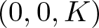 $(0,0,K)$. Moreover, (1) admits a unique positive constant equilibrium
  $(E^*,I^*,S^*)$ if and only if
 \begin{equation}
\mathcal{R}_0:=\frac{\sigma \beta K}{(\sigma + a)(\alpha + a)} \gt 1.
\end{equation}
\begin{equation}
\mathcal{R}_0:=\frac{\sigma \beta K}{(\sigma + a)(\alpha + a)} \gt 1.
\end{equation} In the case 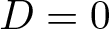 $D=0$, system (1) becomes an ODE model, for which Anderson et al. [Reference Anderson, Jackson, May and Smith1] established the following result: Introducing rabies into a stable population of healthy foxes leads to three possible dynamical outcomes:
(a) If
 $\mathcal{R}_0 \lt 1$, the disease eventually dies out.
(b) If
$\mathcal{R}_0 \gt 1$, the population exhibits oscillations around
$(E^*,I^*,S^*)$; moreover, when the above inequality holds but
$\mathcal R_0$ exceeds
$1$ only slightly, these oscillations are damped over time, and the solution converges to
$(E^*,I^*,S^*)$.(c) In contrast, if
$\mathcal R_0$ is sufficiently large, the system approaches a limit cycle.


The number  $\mathcal R_0$ is widely known as the ‘basic reproduction number’ of the ODE model.
When 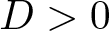 $D \gt 0$, the propagation speed of the epizootic front was investigated in [Reference Murray, Stanley and Brown22] under certain parameter conditions, and the minimal wave speed was analytically derived from fundamental epidemiological and ecological parameters.
In addition, some studies have incorporated the diffusion of juvenile foxes into the model (see, e.g., Ou and Wu [Reference Ou and Wu23]), since juvenile foxes may leave their home range in autumn and disperse over long distances to establish new territories, potentially carrying rabies during such movements.
In general, the mathematical modelling of ecological processes remains highly challenging, largely due to the absence of well-established ‘first principles’ governing their evolutionary mechanisms. As a model describing the evolving rabid fox population with density  $ I(t, x)$, system (1) does not provide enough information for the spatial location of the infected region. For instance, although the initial rabid fox population
 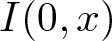 $ I(0, x) $ is naturally assumed to be compactly supported in space, the strong maximum principle implies that
  $ I(t, x) \gt 0 $ for all
  $ x \in \mathbb{R} $ once
  $ t \gt 0 $.
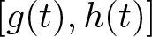
To more accurately characterize the expanding spatial range of rabid foxes, in this paper, we use an evolving one-dimensional interval  $[g(t), h(t)]$ to represent this range, and modify (1) into the following system with moving boundaries:
 \begin{equation}
\left\{\begin{array}{ll}
E_{t}=\beta I S-\sigma E- \left[b+(a-b)\displaystyle\frac{E+I+S}{K}\right]E,\ \ &t \gt 0, \ g(t) \lt x \lt h(t),\\
I_{t}=D I_{xx}+\sigma E-\alpha I- \left[b+(a-b)\displaystyle\frac{E+I+S}{K}\right]I ,\ \ &t \gt 0, \ g(t) \lt x \lt h(t),\\
S_{t}=(a-b)S\left(1-\displaystyle\frac{E+I+S}{K}\right)-\beta I S,\ \ &t \gt 0, \ -\infty \lt x \lt \infty,\\
E(t,x)=I(t,x)=0, & t\geq 0,\ x\not\in (g(t), h(t)), \\
h'(t)=-\mu I_{x}(t,h(t)) , \ &t \gt 0,\\
g'(t)=-\mu I_{x}(t,g(t)), \ &t \gt 0,\\
E(0,x)=E_0(x),\, I(0,x)=I_0(x), \ \ &-h_0\leq x \leq h_0,\\
S(0,x)=S_{0}(x),\, \ \ \ & -\infty \lt x \lt \infty,\\
h(0)=h_0,\,g(0)=-h_0, &
\end{array}\right.
\end{equation}
\begin{equation}
\left\{\begin{array}{ll}
E_{t}=\beta I S-\sigma E- \left[b+(a-b)\displaystyle\frac{E+I+S}{K}\right]E,\ \ &t \gt 0, \ g(t) \lt x \lt h(t),\\
I_{t}=D I_{xx}+\sigma E-\alpha I- \left[b+(a-b)\displaystyle\frac{E+I+S}{K}\right]I ,\ \ &t \gt 0, \ g(t) \lt x \lt h(t),\\
S_{t}=(a-b)S\left(1-\displaystyle\frac{E+I+S}{K}\right)-\beta I S,\ \ &t \gt 0, \ -\infty \lt x \lt \infty,\\
E(t,x)=I(t,x)=0, & t\geq 0,\ x\not\in (g(t), h(t)), \\
h'(t)=-\mu I_{x}(t,h(t)) , \ &t \gt 0,\\
g'(t)=-\mu I_{x}(t,g(t)), \ &t \gt 0,\\
E(0,x)=E_0(x),\, I(0,x)=I_0(x), \ \ &-h_0\leq x \leq h_0,\\
S(0,x)=S_{0}(x),\, \ \ \ & -\infty \lt x \lt \infty,\\
h(0)=h_0,\,g(0)=-h_0, &
\end{array}\right.
\end{equation}where  $\mu$ and
  $h_0$ are positive constants. Here,
  $[g(t), h(t)]$ is the infected region at time
  $t$, in which
  $I$, the rabid foxes, are diffusive, and
  $S$ gets infected by
  $I$ to become
  $E$. The expansion of
  $[g(t), h(t)]$ is driven solely by
  $I$. Both
  $E$ and
  $I$ are absent (identically 0) outside the infected region
  $[g(t), h(t)]$. On the other hand,
  $S$ is assumed to exist over the entire space
  $\mathbb{R}$.
The moving boundaries  $ x = h(t) $ and
  $ x = g(t) $ are also known as free boundaries; they form part of the unknowns in (3) (apart from
  $E,I, S$). The fifth and sixth equations in (3), which govern the evolution of these free boundaries, coincide with the well-known Stefan condition. Such a boundary condition was applied to model the propagation of an invasive species by Du and Lin [Reference Du and Lin10] within the framework of a KPP-type scalar reaction-diffusion equation, and has since been extended to a broad range of problems with a single species (see, e.g., [Reference Du and Guo6–Reference Du and Liang9, Reference Du, Matsuzawa and Zhou12, Reference Kaneko, Matsuzawa and Yamada15, Reference Li, Liang and Shen17, Reference Peng and Zhao24, Reference Wang30]). A deduction of the Stefan condition from some plausible biological assumptions can be found in [Reference Bunting, Du and Krakowski2]. Related free boundary models for multi-species systems of Lotka–Volterra type can be found in [Reference Du and Lin11, Reference Guo and Wu13, Reference Wang29, Reference Wang and Zhang31–Reference Wang and Zhao33, Reference Wang, Qin and Wu37], some similar free boundary systems for epidemic models may be found in [Reference Lin and Zhu18, Reference Wang and Du34, Reference Wang, Nie and Du36] and the associated literature. See also [Reference Du4] for a review.
We note that system (3) differs significantly from the above-mentioned free boundary systems in that two equations in (3) have no diffusion term, and interact nontrivially with a single reaction diffusion equation with free boundaries, which are shared with one of the ODEs in the system. This unusual feature of (3) causes many technical difficulties in the mathematical treatment.
Throughout this paper, the initial functions  $E_0(x)$,
  $I_0(x)$ and
  $S_0(x)$ in (3) are assumed to satisfy
 \begin{equation}
\begin{cases}
E_0\in {\rm Lip}([-h_0,h_0]), E_0(-h_0)=E_0(h_0)=0 \,\text{and } E_0(x) \gt 0 \text{ in } (-h_0,h_0);\\
I_0\in C^{2}([-h_0,h_0]), I_0(\pm h_0)=0, I_0'(-h_0) \gt 0 \gt I_0'(h_0) \ {\rm and}\ I_0(x) \gt 0 \\
\quad {\rm in}\ (-h_0,h_0);\\
S_0\in {\rm Lip}(\mathbb{R}),
0 \lt S_0(x)\leq K\ {\rm in}\ (-\infty, \infty).
\end{cases}
\end{equation}
\begin{equation}
\begin{cases}
E_0\in {\rm Lip}([-h_0,h_0]), E_0(-h_0)=E_0(h_0)=0 \,\text{and } E_0(x) \gt 0 \text{ in } (-h_0,h_0);\\
I_0\in C^{2}([-h_0,h_0]), I_0(\pm h_0)=0, I_0'(-h_0) \gt 0 \gt I_0'(h_0) \ {\rm and}\ I_0(x) \gt 0 \\
\quad {\rm in}\ (-h_0,h_0);\\
S_0\in {\rm Lip}(\mathbb{R}),
0 \lt S_0(x)\leq K\ {\rm in}\ (-\infty, \infty).
\end{cases}
\end{equation}For convenience, we will also write
 \begin{eqnarray*}
\begin{array}{ll}
&f_{1}(E,I,S):=\beta I S-\sigma E- \left[b+(a-b)\displaystyle\frac{E+I+S}{K}\right]E;\ \ \\
&f_{2}(E,I,S):=\sigma E-\alpha I- \left[b+(a-b)\displaystyle\frac{E+I+S}{K}\right]I;\ \ \\
&f_{3}(E,I,S):=(a-b)S\left(1-\displaystyle\frac{E+I+S}{K}\right)-\beta I S.\ \
\end{array}
\end{eqnarray*}
\begin{eqnarray*}
\begin{array}{ll}
&f_{1}(E,I,S):=\beta I S-\sigma E- \left[b+(a-b)\displaystyle\frac{E+I+S}{K}\right]E;\ \ \\
&f_{2}(E,I,S):=\sigma E-\alpha I- \left[b+(a-b)\displaystyle\frac{E+I+S}{K}\right]I;\ \ \\
&f_{3}(E,I,S):=(a-b)S\left(1-\displaystyle\frac{E+I+S}{K}\right)-\beta I S.\ \
\end{array}
\end{eqnarray*} The local existence and uniqueness of solutions to system (3) are established in Section 2 by employing several novel techniques (including applying the Banach fixed point theorem in combination with a parameterized ODE analysis), and then the local solution is uniquely extended to all time  $t \gt 0$ by deriving suitable a priori bounds for the solution; the main results are stated in Theorems 2.1 and 2.2.
The long-time dynamics of (3) is considered in Section 3, based on the comparison principle and the analysis of some associated eigenvalue problems. It is easily seen by the Hopf boundary lemma that  $h'(t) \gt 0 \gt g'(t)$ for
  $t \gt 0$, and hence the following limits always exist:
 \begin{equation*}h_\infty:=\lim_{t\to\infty} h(t)\in (h_0,\infty],~~ g_\infty:=\lim_{t\to\infty} g(t)\in [-\infty, -h_0).\end{equation*}
We have either
 \begin{equation*}
0 \lt h_\infty-g_\infty \lt \infty\ \text{or}\ h_{\infty}-g_\infty =\infty.
\end{equation*}
\begin{equation*}
0 \lt h_\infty-g_\infty \lt \infty\ \text{or}\ h_{\infty}-g_\infty =\infty.
\end{equation*}In the former case, we can show (see Theorem 3.1) that
 \begin{equation*}
(E(t,x), I(t,x), S(t,x))\to (0,0, K) \mbox \ {as}\ t\to\infty.
\end{equation*}
\begin{equation*}
(E(t,x), I(t,x), S(t,x))\to (0,0, K) \mbox \ {as}\ t\to\infty.
\end{equation*}So the rabid foxes vanish eventually, and we will call this the vanishing case.
If  $h_{\infty}-g_\infty =\infty$, a reasonable understanding of the long-time behaviour of (3) is gained when
  $\mathcal R_0 \gt 1$; in this case, we can show that the range of the rabid foxes spread to the entire space
  $\mathbb{ R}$, with density persisting weakly (see Theorem 3.4), namely
 \begin{equation*}
(g_\infty, h_\infty)=(-\infty,\infty) \,\mbox{and } \limsup_{t\to\infty}\min_{x\in [-l, l]}I(t,x) \gt 0\,\mbox{for any } l \gt 0.
\end{equation*}
\begin{equation*}
(g_\infty, h_\infty)=(-\infty,\infty) \,\mbox{and } \limsup_{t\to\infty}\min_{x\in [-l, l]}I(t,x) \gt 0\,\mbox{for any } l \gt 0.
\end{equation*}This will be called the spreading case in this paper.
Thus, in the parameter regime that  $\mathcal R_0 \gt 1$, the long-time dynamics of the model are governed by a spreading-vanishing dichotomy, according to whether
 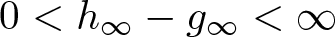 $0 \lt h_\infty-g_\infty \lt \infty$ or
  $h_{\infty}-g_\infty =\infty$.
We believe that strong persistence of  $I$ holds in the spreading case, namely we believe the following conclusions should be true:
 \begin{equation*}
(g_\infty, h_\infty)=(-\infty,\infty)\,\mbox{and } \liminf_{t\to\infty}\min_{x\in [-l, l]}I(t,x) \gt 0\,\mbox{for any } l \gt 0,
\end{equation*}
\begin{equation*}
(g_\infty, h_\infty)=(-\infty,\infty)\,\mbox{and } \liminf_{t\to\infty}\min_{x\in [-l, l]}I(t,x) \gt 0\,\mbox{for any } l \gt 0,
\end{equation*}but we have been unable to prove it, mainly due to the lack of compactness of the solutions  $\{(E(t,\cdot), S(t,\cdot)): t \gt 0\}$ in a suitable function space, caused by the lack of enough regularity of the ODE solutions in the system. This question is left as an open problem at the end of the paper.
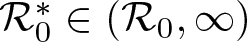
Some easy-to-check sufficient conditions for vanishing and spreading are obtained with the help of certain associated eigenvalue problems, and the results are summarized below (which follow directly from Theorems 3.2, 3.3, 3.4, 3.5, and 3.6):
Let  $(E,I,S,g,h)$ be the solution of (3), and
 \begin{equation*}
\mathcal{R}_0^*:=\displaystyle\frac{\beta\sigma K}{(\alpha+b)(\sigma+b)}.
\end{equation*}
\begin{equation*}
\mathcal{R}_0^*:=\displaystyle\frac{\beta\sigma K}{(\alpha+b)(\sigma+b)}.
\end{equation*}Then we have the following conclusions:
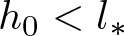
(i) If
$\mathcal R_0^*\leq 1$, then vanishing always happens.(ii) If
$\mathcal R_0^* \gt 1$ and
$l_*$ is given by
then vanishing happens if
\begin{equation*}
l_*:=l(b)=\displaystyle\frac{\pi}{2}\sqrt{\frac{D(\sigma+b)}{\sigma \beta K-(\alpha+b)(\sigma+b)}},
\end{equation*}
$h_0 \lt l_*$ and
$\mu$ is sufficiently small
$($depending on
$E_0, I_0, S_0)$.(iii) If
$\mathcal R_0 \gt 1$ and
$\tilde l_*$ is given by
then spreading always occurs when
\begin{equation*}
\tilde l_*:=l(a)=\displaystyle\frac{\pi}{2}\sqrt{\frac{D(\sigma+a)}{\sigma \beta K-(\alpha+a)(\sigma+a)}},
\end{equation*}
$h_0\geq \tilde l_*$, and when
$h_0 \lt \tilde l_*$, spreading occurs for all sufficiently large
$\mu \ ($depending on
$E_0$,
$I_0$ and
$S_0)$.


2. Existence and uniqueness of a global solution
In this section, we first establish the local existence and uniqueness of solutions to the system (3). Subsequently, by deriving suitable a priori estimates, we show that the local solution can be extended globally. For convenience, we denote
 \begin{eqnarray*}
\Pi:=\{a, b, D,\alpha, \beta, \sigma, \mu, h_0, \|E_0\|_{{\rm Lip}([-h_0,h_0])},\|I_0\|_{C^2([-h_0,h_0])},\|S_0\|_{{\rm Lip}(\mathbb{R})}\}.
\end{eqnarray*}
\begin{eqnarray*}
\Pi:=\{a, b, D,\alpha, \beta, \sigma, \mu, h_0, \|E_0\|_{{\rm Lip}([-h_0,h_0])},\|I_0\|_{C^2([-h_0,h_0])},\|S_0\|_{{\rm Lip}(\mathbb{R})}\}.
\end{eqnarray*}Theorem 2.1. For any given  $(E_0, I_0, S_0)$ satisfying (4) and any
  $\gamma\in(0,1)$, there exists
  $T \gt 0$ depending on
  $\Pi$ and
  $\gamma$ such that problem (3) admits a unique solution
  $(E,I,S,h,g)$ for
  $t\in [0, T]$ with
  $g,h\in C^{\frac{3+ \gamma }{2}}((0,T])\cap C^1([0,T])$ and
 \begin{align*}
&E\in C^{1}([0,T]; L^{\infty}(\mathbb{ R})),\ I\in C^{1+\frac{\gamma}{2}, 2+\gamma}(\Sigma_{T})\cap C^{(1+\gamma)/2, 1+\gamma}(\overline{\Sigma}_{T}),\\
&\quad S\in C^{1}([0,T]; L^{\infty}(\mathbb{R})),\ \end{align*}
\begin{align*}
&E\in C^{1}([0,T]; L^{\infty}(\mathbb{ R})),\ I\in C^{1+\frac{\gamma}{2}, 2+\gamma}(\Sigma_{T})\cap C^{(1+\gamma)/2, 1+\gamma}(\overline{\Sigma}_{T}),\\
&\quad S\in C^{1}([0,T]; L^{\infty}(\mathbb{R})),\ \end{align*}where
 \begin{equation*}
\Sigma_T=\Sigma_{T,g,h}:=\left\{(t,x)\in \mathbb{ R}^{2}:\ t\in(0,T],\ g(t)\leq x\leq h(t)\right\}.
\end{equation*}
\begin{equation*}
\Sigma_T=\Sigma_{T,g,h}:=\left\{(t,x)\in \mathbb{ R}^{2}:\ t\in(0,T],\ g(t)\leq x\leq h(t)\right\}.
\end{equation*} Moreover, there exists  $C \gt 0$ depending on
  $\Pi$ and
  $\gamma$, such that
 \begin{eqnarray*}
\sup_{x\in \mathbb{ R}}\|(E(\cdot,x), S(\cdot,x))\|_{C^1([0,T])}+\|I\|_{C^{(1+\gamma)/2, 1+\gamma}(\overline{\Sigma}_{T})}+\|(g,h)\|_{C^{1+\gamma/2}([0, T])}\leq C.
\end{eqnarray*}
\begin{eqnarray*}
\sup_{x\in \mathbb{ R}}\|(E(\cdot,x), S(\cdot,x))\|_{C^1([0,T])}+\|I\|_{C^{(1+\gamma)/2, 1+\gamma}(\overline{\Sigma}_{T})}+\|(g,h)\|_{C^{1+\gamma/2}([0, T])}\leq C.
\end{eqnarray*}Proof. For clarity, we divide the rather involved proof into several steps. Some ideas in nonlocal diffusion models with free boundary (see, e.g., [Reference Cao, Du, Li and Li3]) will be adapted and used here.
Step 1. Some notations.
Let  $\displaystyle T_1:= \frac{3h_0}{2(2+|g^{*}|+|h^{*}|)}$ with
  $h^{*}:=-\mu I_0'(h_0) \gt 0$,
  $g^{*}:=-\mu I_0'(-h_0) \lt 0$.
For  $0 \lt T\leq T_1$, define
 \begin{align*}
Y_{1,T}&:= \{g\in C^{1}([0, T]):\, g(0)=-h_0,\ g'(0)=g^*,\ g'(t)\leq \frac{g^*}{7}\,\text{for } t\in[0,T],\\ &\quad \|g'-g^*\|_{C([0,T])}\leq 1\},\\[1mm]
Y_{2,T}&:= \{h\in C^{1}([0, T]):\, h(0)=h_0,\ h'(0)=h^*,\ h'(t)\geq \frac{h^*}{7}\,\text{for } t\in[0,T],\\ &\quad \|h'-h^*\|_{C([0,T])}\leq 1\}.
\end{align*}
\begin{align*}
Y_{1,T}&:= \{g\in C^{1}([0, T]):\, g(0)=-h_0,\ g'(0)=g^*,\ g'(t)\leq \frac{g^*}{7}\,\text{for } t\in[0,T],\\ &\quad \|g'-g^*\|_{C([0,T])}\leq 1\},\\[1mm]
Y_{2,T}&:= \{h\in C^{1}([0, T]):\, h(0)=h_0,\ h'(0)=h^*,\ h'(t)\geq \frac{h^*}{7}\,\text{for } t\in[0,T],\\ &\quad \|h'-h^*\|_{C([0,T])}\leq 1\}.
\end{align*} Step 2. Transformation of problem (3) for given  $(g,h)\in T_{1,T}\times Y_{2,T}$.
We consider the transformation 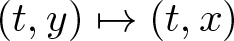 $(t,y)\mapsto(t,x)$ defined by
 \begin{equation*}
x=\Psi(t,y):=\frac{g(t)+h(t)+y(h(t)-g(t))}{2} \quad \text{for } y\in\mathbb{R}.
\end{equation*}
\begin{equation*}
x=\Psi(t,y):=\frac{g(t)+h(t)+y(h(t)-g(t))}{2} \quad \text{for } y\in\mathbb{R}.
\end{equation*} For any fixed  $t\in[0,T]$, it is easily seen that
  $\Psi$ is a diffeomorphism on
  $\mathbb{R}$ due to
  $T\in \left.(0, T_1\right]$ (which implies
  $h(t)-g(t)\geq h_0/2$ for
  $t\in[0,T]$).
By direct calculations, one has
 \begin{equation}
\begin{cases}
\displaystyle\frac{\partial y}{\partial x}&=\displaystyle\frac{2}{h(t)-g(t)}:=\rho(t)=\rho_{g,h}(t), \qquad \displaystyle\frac{\partial^2 y}{\partial x^2}=0, \\
\displaystyle\frac{\partial y}{\partial t}&=\displaystyle\frac{-(h(t)-g(t))(h'(t)+g'(t))-(h'(t)-g'(t))(2x-g(t)-h(t))}{(h(t)-g(t))^2}\\
&=-\displaystyle\frac{h'(t)+g'(t)}{h(t)-g(t)}-\displaystyle\frac{h'(t)-g'(t)}{h(t)-g(t)}y:=-\zeta(t,y)=-\zeta_{g,h}(t,y).\\
\end{cases}
\end{equation}
\begin{equation}
\begin{cases}
\displaystyle\frac{\partial y}{\partial x}&=\displaystyle\frac{2}{h(t)-g(t)}:=\rho(t)=\rho_{g,h}(t), \qquad \displaystyle\frac{\partial^2 y}{\partial x^2}=0, \\
\displaystyle\frac{\partial y}{\partial t}&=\displaystyle\frac{-(h(t)-g(t))(h'(t)+g'(t))-(h'(t)-g'(t))(2x-g(t)-h(t))}{(h(t)-g(t))^2}\\
&=-\displaystyle\frac{h'(t)+g'(t)}{h(t)-g(t)}-\displaystyle\frac{h'(t)-g'(t)}{h(t)-g(t)}y:=-\zeta(t,y)=-\zeta_{g,h}(t,y).\\
\end{cases}
\end{equation}Now we define
 \begin{equation*}
(z_1,z_2,z_3)(t,y):=(E,I,S)(t,x)\,\mbox{for } (t,x)\in \Sigma_T.
\end{equation*}
\begin{equation*}
(z_1,z_2,z_3)(t,y):=(E,I,S)(t,x)\,\mbox{for } (t,x)\in \Sigma_T.
\end{equation*} Then system (3) for  $0 \lt t\leq T$ can be equivalently reformulated as the following two subsystems:
 \begin{equation}
\left\{\begin{array}{ll}
E_t=f_1(E,I,S),\ &0 \lt t\leq T,\ g(t) \lt x \lt h(t), \\
S_t=f_3(E,I,S),\ &0 \lt t\leq T,\ x\in \mathbb{R}, \\
E(t,x)=0,\ & 0 \lt t\leq T, \ x\not\in(g(t),h(t)),\\
E(0,x)=E_0(x),\ &-h_0 \lt x \lt h_0, \\
S(0,x)=S_0(x),\ &x\in \mathbb{R}\\
\end{array}\right.
\end{equation}
\begin{equation}
\left\{\begin{array}{ll}
E_t=f_1(E,I,S),\ &0 \lt t\leq T,\ g(t) \lt x \lt h(t), \\
S_t=f_3(E,I,S),\ &0 \lt t\leq T,\ x\in \mathbb{R}, \\
E(t,x)=0,\ & 0 \lt t\leq T, \ x\not\in(g(t),h(t)),\\
E(0,x)=E_0(x),\ &-h_0 \lt x \lt h_0, \\
S(0,x)=S_0(x),\ &x\in \mathbb{R}\\
\end{array}\right.
\end{equation}and
 \begin{equation}
\left\{\begin{array}{ll}
z_{2t}-D\rho^{2}z_{2yy}-\zeta z_{2y}=f_2(z_1,z_2,z_3),\ & 0 \lt t\leq T,\ |y| \lt 1, \\
z_{2}(t,1)=z_{2}(t,-1)=0,\ &0 \lt t\leq T, \\
h'(t)=-\mu\rho z_{2y}(t,1),\ &0 \lt t\leq T, \\
g'(t)=-\mu\rho z_{2y}(t,-1),\ & 0 \lt t\leq T, \\
z_{2}(0,y)=I_{0}(h_{0}y)=:z_{20}(y), \ & |y| \lt 1,\\
g(0)=-h_0,\ h(0)=h_0.
\end{array}\right.
\end{equation}
\begin{equation}
\left\{\begin{array}{ll}
z_{2t}-D\rho^{2}z_{2yy}-\zeta z_{2y}=f_2(z_1,z_2,z_3),\ & 0 \lt t\leq T,\ |y| \lt 1, \\
z_{2}(t,1)=z_{2}(t,-1)=0,\ &0 \lt t\leq T, \\
h'(t)=-\mu\rho z_{2y}(t,1),\ &0 \lt t\leq T, \\
g'(t)=-\mu\rho z_{2y}(t,-1),\ & 0 \lt t\leq T, \\
z_{2}(0,y)=I_{0}(h_{0}y)=:z_{20}(y), \ & |y| \lt 1,\\
g(0)=-h_0,\ h(0)=h_0.
\end{array}\right.
\end{equation}Step 3. An extension trick.
For  $T\in \left.(0, T_1\right]$ define
  $D_T=[0,T]\times [-1,1]$ and
 \begin{align*}
Y_{3,T}:=\Big\{z_2\in C(D_{T}): & z_2\geq 0\,\text{in } D_{T},\, z_2(0,y)=z_{20}(y),\, z_2(t,\pm 1)=0, \\
& \,\sup\limits_{-1\leq y_1,y_2\leq 1,t\in[0,T]\atop y_1\neq y_2}\frac{|z_2(t,y_1)-z_2(t,y_2)|}{|y_1-y_2|}\leq B,\\
&\|z_2-z_{20}\|_{C(D_T)}\leq 1
\Big\},
\end{align*}
\begin{align*}
Y_{3,T}:=\Big\{z_2\in C(D_{T}): & z_2\geq 0\,\text{in } D_{T},\, z_2(0,y)=z_{20}(y),\, z_2(t,\pm 1)=0, \\
& \,\sup\limits_{-1\leq y_1,y_2\leq 1,t\in[0,T]\atop y_1\neq y_2}\frac{|z_2(t,y_1)-z_2(t,y_2)|}{|y_1-y_2|}\leq B,\\
&\|z_2-z_{20}\|_{C(D_T)}\leq 1
\Big\},
\end{align*}with  $B \gt 0$ to be specified later. Clearly
 \begin{equation*}
Y_T:=\prod_{i=1}^3 Y_{i,T}
\end{equation*}
\begin{equation*}
Y_T:=\prod_{i=1}^3 Y_{i,T}
\end{equation*}is a complete metric space endowed with the following metric:
 \begin{equation*}
d((g_1,h_1, z_{21}),(g_2,h_2, z_{22}) ):=\|g_1'-g_2'\|_{C([0,T])}+\|h_1'-h_2'\|_{C([0,T])}+\|z_{21}-z_{22}\|_{C(D_T)}.
\end{equation*}
\begin{equation*}
d((g_1,h_1, z_{21}),(g_2,h_2, z_{22}) ):=\|g_1'-g_2'\|_{C([0,T])}+\|h_1'-h_2'\|_{C([0,T])}+\|z_{21}-z_{22}\|_{C(D_T)}.
\end{equation*} With  $0 \lt T \lt T_1$, we define a subspace of
  $Y_{T_1}$, denoted by
  $Y_{T_1}^{T}:=\prod_{i=1}^3 Y_{i,T_1}^{T}$, with
 \begin{align*}
Y^{T}_{1,T_1}&:=\{g\in C^{1}([0, T_1]):\ g|_{[0,T]}\in Y_{1,T},\\
&\quad g(t)=g(T)+g'(T)(t-T)\,\text{for }T\leq t\leq T_1\},\\[1mm]
Y^{T}_{2,T_1}&:=\{h\in C^{1}([0, T_1]):\ h|_{[0,T]}\in Y_{2,T}, \\
&\quad h(t)=h(T)+h'(T)(t-T)\text{for }T\leq t\leq T_1\},\\[1mm]
Y^{T}_{3,T_1}&:=\{z_2\in C(D_{T_1}): z_2|_{[0,T]}\in Y_{3,T},\ z_2(t,y)=z_2(T,y)\text{for }T\leq t\leq T_1 \}.
\end{align*}
\begin{align*}
Y^{T}_{1,T_1}&:=\{g\in C^{1}([0, T_1]):\ g|_{[0,T]}\in Y_{1,T},\\
&\quad g(t)=g(T)+g'(T)(t-T)\,\text{for }T\leq t\leq T_1\},\\[1mm]
Y^{T}_{2,T_1}&:=\{h\in C^{1}([0, T_1]):\ h|_{[0,T]}\in Y_{2,T}, \\
&\quad h(t)=h(T)+h'(T)(t-T)\text{for }T\leq t\leq T_1\},\\[1mm]
Y^{T}_{3,T_1}&:=\{z_2\in C(D_{T_1}): z_2|_{[0,T]}\in Y_{3,T},\ z_2(t,y)=z_2(T,y)\text{for }T\leq t\leq T_1 \}.
\end{align*} It is clear that each element of  $Y_{T}$ can be extended to be an element of
  $Y_{T_1}^T$. As a result, in what follows we will always identify
  $Y_T$ with
  $Y_{T_1}^T$. This extension trick will be used in our proof of local existence to (7).
Step 4. Solving (6) for any given  $(g,h, z_2)\in Y_T=Y_{T_1}^T\subseteq Y_{T_1}$.
By the definition of  $T_1$, we have
 \begin{equation*}
\frac{7h_0}{2}\geq 2h_0+(2+h^*-g^*)T_1\geq h(t)-g(t)\geq 2h_0+(h^*-g^*-2)T_1\geq \frac{h_0}{2}\,\text{for }t\in[0,T_1],
\end{equation*}
\begin{equation*}
\frac{7h_0}{2}\geq 2h_0+(2+h^*-g^*)T_1\geq h(t)-g(t)\geq 2h_0+(h^*-g^*-2)T_1\geq \frac{h_0}{2}\,\text{for }t\in[0,T_1],
\end{equation*}which implies that the map  $y\to x=\Psi(t,y)$ is a diffeomorphism on
  $\mathbb{R}$ for each
  $t\in[0,T_1]$. Therefore, the function
  $I(t,x):=z_2(t,y)$ is well-defined for all
  $(t,x)\in\Sigma_{T_1}$. We extend
  $ I(t,x) $ by zero outside the interval
  $ [g(t), h(t)] $ of
  $x$ for each
  $ t \in [0, T_1] $, and denote the extended function by
  $ \bar{I}(t,x) $.
For any given  $x\in[g(T_1),h(T_1)]$, let
 \begin{eqnarray*}
\begin{array}{l}
\tilde{E}_0(x):=\left\{\begin{array}{ll}
E_0(x),\ &-h_0\leq x\leq h_0, \\
0,\ &x\not\in[-h_0,h_0]
\end{array}\right.
\\
t_{x}:=\left\{\begin{array}{ll}
t_{x}^{g},\ & \text{if }g(T_1)\leq x \lt -h_0\ {\rm and}\ x=g(t_{x}^{g}), \\
0,\ & \text{if }-h_0\leq x\leq h_0, \\
t_{x}^{h},\ &\text{if }h_0 \lt X\leq h(T_1)\ {\rm and}\ x=h(t_{x}^{h}).
\end{array}\right.
\end{array}
\end{eqnarray*}
\begin{eqnarray*}
\begin{array}{l}
\tilde{E}_0(x):=\left\{\begin{array}{ll}
E_0(x),\ &-h_0\leq x\leq h_0, \\
0,\ &x\not\in[-h_0,h_0]
\end{array}\right.
\\
t_{x}:=\left\{\begin{array}{ll}
t_{x}^{g},\ & \text{if }g(T_1)\leq x \lt -h_0\ {\rm and}\ x=g(t_{x}^{g}), \\
0,\ & \text{if }-h_0\leq x\leq h_0, \\
t_{x}^{h},\ &\text{if }h_0 \lt X\leq h(T_1)\ {\rm and}\ x=h(t_{x}^{h}).
\end{array}\right.
\end{array}
\end{eqnarray*} Clearly,  $t_{g(T_1)}=t_{h(T_1)}=T_1$. Moreover, we set
  $t_x=T_1$ for
 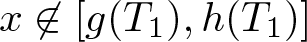 $x\not\in [g(T_1),h(T_1)]$.
We now consider the following ODE problems with parameter  $x$:
$x$:
 \begin{equation}
\left\{\begin{array}{ll}
E_t=f_1(E,\bar{I}(t,x),S),\ E(t_x,x)=\tilde{E}_0(x),\, & t_x \lt t\leq T_1, x\in(g(T_1),h(T_1)), \\
E(t,x)=0, & 0\leq t\leq T_1,\ x\not\in[g(t),h(t)],\\
S_t=f_3(E,\bar{I}(t,x),S),\ S(0,x)=S_0(x),\,& 0 \lt t\leq T_1,\ x\in\mathbb{ R}.
\end{array}\right.
\end{equation}
\begin{equation}
\left\{\begin{array}{ll}
E_t=f_1(E,\bar{I}(t,x),S),\ E(t_x,x)=\tilde{E}_0(x),\, & t_x \lt t\leq T_1, x\in(g(T_1),h(T_1)), \\
E(t,x)=0, & 0\leq t\leq T_1,\ x\not\in[g(t),h(t)],\\
S_t=f_3(E,\bar{I}(t,x),S),\ S(0,x)=S_0(x),\,& 0 \lt t\leq T_1,\ x\in\mathbb{ R}.
\end{array}\right.
\end{equation} Before starting to solve (8), let us note that due to 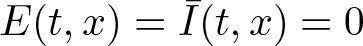 $E(t,x)=\bar{I}(t,x)=0$ for
 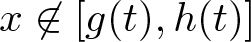 $x\not\in[g(t),h(t)]$, for each
  $x\in \mathbb{ R}\setminus[-h_0,h_0]$, problem (8) reduces to the following single logistic equation for
  $t\in[0,t_x]$:
 \begin{equation}
S_t=(a-b)S(1-\frac{S}{K})\,\text{for } t\in(0,t_x], \quad S(0,x)=S_0(x),
\end{equation}
\begin{equation}
S_t=(a-b)S(1-\frac{S}{K})\,\text{for } t\in(0,t_x], \quad S(0,x)=S_0(x),
\end{equation}which admits a unique solution  $\hat{S}\in C^{1}([0,t_x])$ satisfying
 \begin{equation}
0 \lt \hat{S}(t,x)\leq K\,\text{for }t\in[0,t_x].
\end{equation}
\begin{equation}
0 \lt \hat{S}(t,x)\leq K\,\text{for }t\in[0,t_x].
\end{equation}We are now ready to fully solve (8). Set
 \begin{equation*}
\textbf{V}:=\left(\begin{array}{c}E\\S\end{array}\right)
\text{and }\textbf{F}(t,x,\textbf{V}):=\left(\begin{array}{c}
f_1(E,\bar{I}(t,x),S) \\
f_3(E,\bar{I}(t,x),S)
\end{array}\right).
\end{equation*}
\begin{equation*}
\textbf{V}:=\left(\begin{array}{c}E\\S\end{array}\right)
\text{and }\textbf{F}(t,x,\textbf{V}):=\left(\begin{array}{c}
f_1(E,\bar{I}(t,x),S) \\
f_3(E,\bar{I}(t,x),S)
\end{array}\right).
\end{equation*} Then the pair  $(E,S)$ is a solution to (8) if and only if
  $\mathbf{V}$ is a solution to the following system with parameter
  $x\in\mathbb{ R}$:
 \begin{equation}
\begin{cases}
\textbf{V}_t=\textbf{F}(t,x,\textbf{V}) &\text{for }t\in[t_x,T_1],\\
\textbf{V}(t,x)=\left(\begin{array}{c}
0 \\
\hat{S}(t,x)
\end{array}\right)
&\text{for }t\in[0,t_x].
\end{cases}
\end{equation}
\begin{equation}
\begin{cases}
\textbf{V}_t=\textbf{F}(t,x,\textbf{V}) &\text{for }t\in[t_x,T_1],\\
\textbf{V}(t,x)=\left(\begin{array}{c}
0 \\
\hat{S}(t,x)
\end{array}\right)
&\text{for }t\in[0,t_x].
\end{cases}
\end{equation} Since  $f_1$ and
  $f_3$ are smooth in
  $(E,\bar{I},S)$, and
  $\bar{I}$ is continuous and uniformly bounded, it is easy to verify that
  $\textbf{F}$ is Lipschitz continuous in
  $\textbf{V}\in[0,L_1]^2$, uniformly with respect to
  $(t,x)\in[0,T_1]\times\mathbb{ R}$, where
 \begin{equation*}
L_1:=\max\{K, \|E_0\|_{L^\infty([-h_0,h_0]\|)}+\|S_0\|_{L^\infty(\mathbb{R})}\}.
\end{equation*}
\begin{equation*}
L_1:=\max\{K, \|E_0\|_{L^\infty([-h_0,h_0]\|)}+\|S_0\|_{L^\infty(\mathbb{R})}\}.
\end{equation*} Hence, it follows from the fundamental theorem of ODEs that for each  $x\in\mathbb{ R}$, (11) possesses a unique solution
  $\textbf{V}\in [C^1([t_x,T_x])]^2$ for some
  $T_x\in \left. (t_x, T_1\right]$. Consequently, for each
  $x\in\mathbb{ R}$, (8) has a unique solution
  $(E,S)$ defined on
  $[0,T_x]$.
Next, we show that  $(E,S)$ can be uniquely extended to
  $[0,T_1]$. It suffices to show that for each
  $x\in\mathbb{ R}$ and
  $T_a\in[T_x,T_1]$, if
  $(E,S)$ solves (8) for
  $t\in[0,T_a]$, then
 \begin{equation}
0\leq S(t,x),E(t,x)\leq L_1 \ \text{for } t\in[0,T_a].
\end{equation}
\begin{equation}
0\leq S(t,x),E(t,x)\leq L_1 \ \text{for } t\in[0,T_a].
\end{equation} For each  $x\in\mathbb{ R}$, since
  $E(t,x)=0$ and
  $S(t,x)=\hat{S}(t,x)$ for
  $t\in[0,t_x]$, inequality (12) holds obviously for
  $t\in[0,t_x]$. Hence, it remains to prove (12) for
  $t\in[t_x,T_a]$.
Denote  $X_g:=g(T_a)$ and
  $X_h:=h(T_a)$. If
  $x\in\left. (-\infty,X_g \right]\cup \left[X_h,\infty) \right.$, it is clear that
  $T_a\leq t_x$, and thus (12) already holds. If
  $x\in [X_g, X_h]$, we complete the proof according to two cases.
Case (a):  $x\in(-h_0,h_0)$. For such
  $x$ we have
  $E_0(x),S_0(x) \gt 0$, and it follows by continuity that
  $E(t,x),S(t,x)\geq 0$ for all
  $t\in[0,\tau]$ with some small
  $\tau \gt 0$. Thus, we have
 \begin{equation*}
S_t\leq (a-b)S\left(1-\displaystyle\frac{S}{K}\right) \text{for } t\in(0,\tau],
\end{equation*}
\begin{equation*}
S_t\leq (a-b)S\left(1-\displaystyle\frac{S}{K}\right) \text{for } t\in(0,\tau],
\end{equation*}which combined with  $0 \lt S(0,x) \lt K$ yields
  $0\leq S(t,x) \lt K$ for
  $t\in[0,\tau]$.
Define 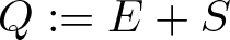 $Q:=E+S$; then
  $Q$ satisfies
 \begin{equation*}\begin{cases}
Q_t=-(\sigma+b)E+(a-b)S-(a-b)\displaystyle\frac{\bar{I}+Q}{K}Q\leq (a-b)Q(1-\frac{Q}{K}), ~~~t\in[0,\tau],\\
Q(0,x)\leq L_1.
\end{cases}
\end{equation*}
\begin{equation*}\begin{cases}
Q_t=-(\sigma+b)E+(a-b)S-(a-b)\displaystyle\frac{\bar{I}+Q}{K}Q\leq (a-b)Q(1-\frac{Q}{K}), ~~~t\in[0,\tau],\\
Q(0,x)\leq L_1.
\end{cases}
\end{equation*} By comparing  $Q$ with
  $L_1$, we deduce that
  $Q(t,x)\leq L_1$ and thus
  $0\leq E(t,x)\leq L_1$ for
  $t\in[0,\tau]$. This establishes (12) for
  $t\in[0,\tau]$.
We now claim that (12) holds for all  $t\in[0,T_a]$. From the arguments above, one obtains that
  $E,S\leq L_1$ as long as
  $E,S\geq 0$. Therefore, it suffices to prove
  $E,S\geq 0$ for
  $t\in[0,T_a]$. Suppose on the contrary that this conclusion does not hold; then there exists a first time moment
  $t^*\in\left. (0,T_a\right]$ such that
  $L_1\geq E(t,x), S(t,x)\geq 0$ for
  $t\in\left. (0,t^* \right]$ and at least one of the following happens:
 \begin{equation*}
{\rm (i)} \ S(t^*,x)=0, \ \
{\rm (ii)}\ E(t^*,x)=0.
\end{equation*}
\begin{equation*}
{\rm (i)} \ S(t^*,x)=0, \ \
{\rm (ii)}\ E(t^*,x)=0.
\end{equation*} However, using (8) we see there are some continuous functions  $C^x_1(t)$ and
  $C^x_2(t)$ such that
 \begin{equation*}
S_t\geq C^x_1(t)S\,\mbox{for } 0=t_x \lt t\leq t^*,\ E_t\geq C^x_2(t)E \ \mbox{for } 0 \lt t\leq t^*.
\end{equation*}
\begin{equation*}
S_t\geq C^x_1(t)S\,\mbox{for } 0=t_x \lt t\leq t^*,\ E_t\geq C^x_2(t)E \ \mbox{for } 0 \lt t\leq t^*.
\end{equation*} These inequalities imply, due to  $E(0,x)=0$ and
  $S(0,x) \gt 0$, that
  $E(t^*,x) \gt 0$ and
  $S(t^*,x) \gt 0$. This contradiction indicates that
  $E,S\geq 0$ for
  $t\in[0,T_a]$ and thus (12) holds.
Case (b):  $x\in \left.(X_g,-h_0\right]\cup \left[h_0,X_h)\right.$. By (10), we see that
  $0 \lt S(t,x)\leq K$ for
  $t\in[0,t_x]$. Let
  $(E_\delta,S_\delta)$ be the solution of
 \begin{equation}
\left\{\begin{array}{ll}
E_t=f_1(E,\bar{I},S),\ & t_x \lt t\leq T_a, \\
S_t=f_3(E,\bar{I},S),\ & t_x \lt t\leq T_a
\end{array}\right.
\end{equation}
\begin{equation}
\left\{\begin{array}{ll}
E_t=f_1(E,\bar{I},S),\ & t_x \lt t\leq T_a, \\
S_t=f_3(E,\bar{I},S),\ & t_x \lt t\leq T_a
\end{array}\right.
\end{equation}with initial conditions
 \begin{equation*}
E_\delta(t_x,x)=\delta,~S_\delta(t_x,x)=S(t_x,x),
\end{equation*}
\begin{equation*}
E_\delta(t_x,x)=\delta,~S_\delta(t_x,x)=S(t_x,x),
\end{equation*}where  $\delta \gt 0$ is a small constant. By the continuous dependence of solutions for ODE on initial values, we know that
  $(E_{\delta}, S_\delta)$ is well-defined in
  $[t_x,T_a]$ for all small
  $\delta \gt 0$, and
 \begin{equation*}E(t,x)=\lim_{\delta\to 0}E_\delta(t,x),\ S(t,x)=\lim_{\delta\to 0}S_\delta(t,x)\,\text{uniformly for } t\in[t_x,T_a].\end{equation*}
 Using arguments similar to those of Case (1), we have  $E_{\delta}(t,x), S_\delta(t,x) \gt 0$ for
  $t\in[t_x,T_a]$. Hence,
  $E(t,x),S(t,x)\geq 0$ for
  $t\in[t_x,T_a]$.
Consequently, for any given  $(g,h, z_2)\in Y_T=Y_{T_1}^T\subseteq Y_{T_1}$ and fixed
  $x\in\mathbb{R}$, (8) admits a unique solution
  $(E(\cdot, x),S(\cdot, x))\in C^{1}([0,T_1])\times C^{1}([0,T_1])$, and
 \begin{eqnarray*}
0\leq E(t,x),S(t,x)\leq L_1 \quad \text{for }t\in[0,T_1],\ x\in\mathbb{ R},
\end{eqnarray*}
\begin{eqnarray*}
0\leq E(t,x),S(t,x)\leq L_1 \quad \text{for }t\in[0,T_1],\ x\in\mathbb{ R},
\end{eqnarray*}which induces a nonlinear mapping  $\mathcal{N}:Y_T\to \left[C^1([0,T_1];L^\infty(\mathbb{ R}))\right]^2$ given by
 \begin{equation}
\mathcal{N}(g,h, z_2) = (E,S).
\end{equation}
\begin{equation}
\mathcal{N}(g,h, z_2) = (E,S).
\end{equation} Step 5: We show that  $(E,S)=\mathcal{N}(g,h, z_2)\in {\rm Lip}([0,T_1]\times\mathbb{ R})$.
Since  $\bar{I}(t,x)=E(t,x)=0$ for
  $t\in [0, T_1]$,
  $x\not\in [g(t),h(t)]$, it is easily seen that, for every
  $x\in\mathbb{ R}$,
 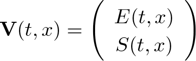 $\textbf{V}(t,x)=\left(\begin{array}{c}
E(t,x) \\
S(t,x)
\end{array}\right)
$ satisfies
$\textbf{V}(t,x)=\left(\begin{array}{c}
E(t,x) \\
S(t,x)
\end{array}\right)
$ satisfies
 \begin{equation*}
\textbf{V}_t=\textbf{F}(t,x,\textbf{V}) \ \text{for } t\in[0,T], \quad \textbf{V}(0,x)=\textbf{V}_0(x):=\left(\begin{array}{c}
\tilde E_0(x) \\
S_0(x)
\end{array}\right),
\end{equation*}
\begin{equation*}
\textbf{V}_t=\textbf{F}(t,x,\textbf{V}) \ \text{for } t\in[0,T], \quad \textbf{V}(0,x)=\textbf{V}_0(x):=\left(\begin{array}{c}
\tilde E_0(x) \\
S_0(x)
\end{array}\right),
\end{equation*}which is equivalent to the integral equation
 \begin{equation}
\textbf{V}(t,x)= \textbf{V}_0(x)+\int_0^t\textbf{F}(\tau,x,\textbf{V}(\tau,x))d\tau \ \text{for }t\in[0,T],\ x\in\mathbb{ R}.
\end{equation}
\begin{equation}
\textbf{V}(t,x)= \textbf{V}_0(x)+\int_0^t\textbf{F}(\tau,x,\textbf{V}(\tau,x))d\tau \ \text{for }t\in[0,T],\ x\in\mathbb{ R}.
\end{equation} Since  $f_1$ and
  $f_3$ are smooth, by (12) and the choice of
  $\bar{I}$, there exists a constant
  $N_1 \gt 0$ such that, for any
  $t\in[0,T_1]$ and
  $x_1,x_2\in\mathbb{ R}$,
 \begin{equation}\begin{cases}
|\textbf{F}(t,x_1,\textbf{V}(t,x_1))-\textbf{F}(t,x_1,\textbf{V}(t,x_2))|\leq N_1|\textbf{V}(t,x_1)-\textbf{V}(t,x_2)|,\\
|\textbf{F}(t,x_1,\textbf{V}(t,x_2))- \textbf{F}(t,x_2,\textbf{V}(t,x_2))|\leq N_1|\bar{I}(t,x_1)-\bar{I}(t,x_2)|.
\end{cases}
\end{equation}
\begin{equation}\begin{cases}
|\textbf{F}(t,x_1,\textbf{V}(t,x_1))-\textbf{F}(t,x_1,\textbf{V}(t,x_2))|\leq N_1|\textbf{V}(t,x_1)-\textbf{V}(t,x_2)|,\\
|\textbf{F}(t,x_1,\textbf{V}(t,x_2))- \textbf{F}(t,x_2,\textbf{V}(t,x_2))|\leq N_1|\bar{I}(t,x_1)-\bar{I}(t,x_2)|.
\end{cases}
\end{equation}It then follows from (15) that
 \begin{align*}
&|\textbf{V}(t,x_1)-\textbf{V}(t,x_2)|\\
\leq&\ |\textbf{V}_0(x_1)-\textbf{V}_0(x_2)|+\int_0^t|F(\tau,x_1,\textbf{V}(\tau,x_1))-F(\tau,x_2,\textbf{V}(\tau,x_2))|d\tau\\
\leq&\ |\textbf{V}_0(x_1)-\textbf{V}_0(x_2)|+N_1\int_0^t(|\bar{I}(\tau,x_1)-\bar{I}(\tau,x_2)|+|\textbf{V}(\tau,x_1)-\textbf{V}(\tau,x_2)|)d\tau\\
\leq&\ \left([\textbf{V}_0]_{{\rm Lip}(\mathbb{ R})}+N_1T_1\sup_{t\in[0,T_1]}[\bar{I}(t,\cdot)]_{{\rm Lip}(\mathbb{ R})}\right)|x_1-x_2|\\
&\quad +N_1\int_0^t|\textbf{V}(\tau,x_1)-\textbf{V}(\tau,x_2)|d\tau.
\end{align*}
\begin{align*}
&|\textbf{V}(t,x_1)-\textbf{V}(t,x_2)|\\
\leq&\ |\textbf{V}_0(x_1)-\textbf{V}_0(x_2)|+\int_0^t|F(\tau,x_1,\textbf{V}(\tau,x_1))-F(\tau,x_2,\textbf{V}(\tau,x_2))|d\tau\\
\leq&\ |\textbf{V}_0(x_1)-\textbf{V}_0(x_2)|+N_1\int_0^t(|\bar{I}(\tau,x_1)-\bar{I}(\tau,x_2)|+|\textbf{V}(\tau,x_1)-\textbf{V}(\tau,x_2)|)d\tau\\
\leq&\ \left([\textbf{V}_0]_{{\rm Lip}(\mathbb{ R})}+N_1T_1\sup_{t\in[0,T_1]}[\bar{I}(t,\cdot)]_{{\rm Lip}(\mathbb{ R})}\right)|x_1-x_2|\\
&\quad +N_1\int_0^t|\textbf{V}(\tau,x_1)-\textbf{V}(\tau,x_2)|d\tau.
\end{align*}Because
 \begin{align*}
&\sup_{t\in[0,T_1]}[\bar{I}(t,\cdot)]_{{\rm Lip}(\mathbb{ R})}=\sup_{t\in[0,T_1]}[I(t,\cdot)]_{{\rm Lip}([g(t),h(t)])}\\
=&\sup_{t\in[0,T_1],x_1,x_2\in[g(t),h(t)]\atop x_1\neq x_2} \frac{|z_2(t,\Psi^{-1}(t,x_1))-z_2(t,\Psi^{-1}(t,x_2))|}{x_1-x_2}\\
\leq& \sup_{t\in[0,T_1],x_1,x_2\in[g(t),h(t)]\atop x_1\neq x_2}\left([z(t,\cdot)]_{{\rm Lip}([-1,1])}\frac{|\Psi^{-1}(t,x_1)-\Psi^{-1}(t,x_2)|}{x_1-x_2}\right)\leq \frac{4B}{h_0},
\end{align*}
\begin{align*}
&\sup_{t\in[0,T_1]}[\bar{I}(t,\cdot)]_{{\rm Lip}(\mathbb{ R})}=\sup_{t\in[0,T_1]}[I(t,\cdot)]_{{\rm Lip}([g(t),h(t)])}\\
=&\sup_{t\in[0,T_1],x_1,x_2\in[g(t),h(t)]\atop x_1\neq x_2} \frac{|z_2(t,\Psi^{-1}(t,x_1))-z_2(t,\Psi^{-1}(t,x_2))|}{x_1-x_2}\\
\leq& \sup_{t\in[0,T_1],x_1,x_2\in[g(t),h(t)]\atop x_1\neq x_2}\left([z(t,\cdot)]_{{\rm Lip}([-1,1])}\frac{|\Psi^{-1}(t,x_1)-\Psi^{-1}(t,x_2)|}{x_1-x_2}\right)\leq \frac{4B}{h_0},
\end{align*}it follows from Gronwall’s inequality that
 \begin{align}
&|\textbf{V}(t,x_1)-\textbf{V}(t,x_2)|\leq (1+N_1T_1e^{N_1T_1})\left(\|\textbf{V}_0\|_{{\rm Lip}(\mathbb{ R})}+\frac{4N_1T_1B}{h_0}\right)|x_1-x_2| \nonumber\\
&\quad := K_1 |x_1-x_2|.
\end{align}
\begin{align}
&|\textbf{V}(t,x_1)-\textbf{V}(t,x_2)|\leq (1+N_1T_1e^{N_1T_1})\left(\|\textbf{V}_0\|_{{\rm Lip}(\mathbb{ R})}+\frac{4N_1T_1B}{h_0}\right)|x_1-x_2| \nonumber\\
&\quad := K_1 |x_1-x_2|.
\end{align} Similarly, there exists a constant  $K_2 \gt 0$ depending on
  $L_1$ and
  $\Pi$ such that
 \begin{equation*}
|\textbf{V}(t,x_2)-\textbf{V}(s,x_2)|\leq K_2 |t-s|\,\mbox{for all } t,s \in [0,T_{1}],\ x_2\in\mathbb{R}.
\end{equation*}
\begin{equation*}
|\textbf{V}(t,x_2)-\textbf{V}(s,x_2)|\leq K_2 |t-s|\,\mbox{for all } t,s \in [0,T_{1}],\ x_2\in\mathbb{R}.
\end{equation*}As a result, we conclude that
 \begin{align*}
&\|\textbf{V}\|_{{\rm Lip}([0,T_1]\times\mathbb{ R})}=\|\textbf{V}\|_{L^\infty([0,T_1]\times\mathbb{ R})}+[\textbf{V}]_{{\rm Lip}([0,T_1]\times \mathbb{ R})}\\
\leq&\ \|\textbf{V}\|_{L^\infty([0,T_1]\times\mathbb{ R})}+\sup_{t\in[0,T_1],x_1,x_2\in\mathbb{ R}\atop x_1\neq x_2}\frac{|\textbf{V}(t,x_1)-\textbf{V}(t,x_2)|}{|x_1-x_2|}\\
&\quad +\sup_{(t,s)\in[0,T_1],x_2\in\mathbb{ R}\atop t\neq s}\frac{|\textbf{V}(t,x_2)-\textbf{V}(s,x_2)|}{|t-s|}\\
\leq&\ L_1+K_1+2K_2 \lt \infty,
\end{align*}
\begin{align*}
&\|\textbf{V}\|_{{\rm Lip}([0,T_1]\times\mathbb{ R})}=\|\textbf{V}\|_{L^\infty([0,T_1]\times\mathbb{ R})}+[\textbf{V}]_{{\rm Lip}([0,T_1]\times \mathbb{ R})}\\
\leq&\ \|\textbf{V}\|_{L^\infty([0,T_1]\times\mathbb{ R})}+\sup_{t\in[0,T_1],x_1,x_2\in\mathbb{ R}\atop x_1\neq x_2}\frac{|\textbf{V}(t,x_1)-\textbf{V}(t,x_2)|}{|x_1-x_2|}\\
&\quad +\sup_{(t,s)\in[0,T_1],x_2\in\mathbb{ R}\atop t\neq s}\frac{|\textbf{V}(t,x_2)-\textbf{V}(s,x_2)|}{|t-s|}\\
\leq&\ L_1+K_1+2K_2 \lt \infty,
\end{align*}which indicates that  $E,S\in {\rm Lip}([0,T_1]\times\mathbb{ R}).$
Step 6: We solve a linear parabolic problem arising from (7).
For given  $(g,h, z_2)\in Y_T=Y_{T_1}^T$, from Step 4 we obtain the solution
 \begin{equation*}
(E, S)=\mathcal N(g,h,z_2).
\end{equation*}
\begin{equation*}
(E, S)=\mathcal N(g,h,z_2).
\end{equation*} Recalling the notation  $z_1(t,y)=E(t,x)$ and
  $z_3(t,y)=S(t,x)$ for
  $(t,x)\in\Sigma_{T_1}$, and our estimate
 \begin{equation*}
0\leq z_1(t,y),z_3(t,y)\leq L_1\,\text{for }(t,y)\in D_{T_1},
\end{equation*}
\begin{equation*}
0\leq z_1(t,y),z_3(t,y)\leq L_1\,\text{for }(t,y)\in D_{T_1},
\end{equation*}we now set to solve the following linear parabolic initial boundary value problem:
 \begin{equation}
\left\{\begin{array}{ll}
\tilde{z}_{2t}-D\rho^{2}\tilde{z}_{2yy}-D\zeta \tilde{z}_{2y}=f_2(z_1,z_2,z_3),\ &t \gt 0,\ y\in[-1,1], \\
\tilde{z}_{2}(t,\pm 1)=0,\ &t\geq 0, \\
\tilde{z}_{2}(0,y)=I_{0}(h_{0}y):=z_{20}(y), \ & y\in[-1,1].
\end{array}\right.
\end{equation}
\begin{equation}
\left\{\begin{array}{ll}
\tilde{z}_{2t}-D\rho^{2}\tilde{z}_{2yy}-D\zeta \tilde{z}_{2y}=f_2(z_1,z_2,z_3),\ &t \gt 0,\ y\in[-1,1], \\
\tilde{z}_{2}(t,\pm 1)=0,\ &t\geq 0, \\
\tilde{z}_{2}(0,y)=I_{0}(h_{0}y):=z_{20}(y), \ & y\in[-1,1].
\end{array}\right.
\end{equation} By the expressions of  $\rho$ and
  $\zeta$ given in (5), we can calculate to obtain that
 \begin{equation}
\frac{D}{4h_0^2}\leq D\rho^2(g(t),h(t))\leq \frac{16D}{h_0^2}\,\mbox{for } (t,y)\in D_{T_1},
\end{equation}
\begin{equation}
\frac{D}{4h_0^2}\leq D\rho^2(g(t),h(t))\leq \frac{16D}{h_0^2}\,\mbox{for } (t,y)\in D_{T_1},
\end{equation} \begin{equation}
\begin{aligned}
\|\zeta\|_{C(D_{T_1})}
\leq &\sup_{(t,x)\in D_{T_1}}\left|\frac{h'(t)+g'(t)}{h(t)-g(t)}\right|+ \sup_{(t,x)\in D_{T_1}}\left|\frac{(h'(t)-g'(t))y}{h(t)-g(t)}\right|\\
\leq &\ \frac{4(|g^*|+|h^*|+2)}{h_0}:=C_0.
\end{aligned}
\end{equation}
\begin{equation}
\begin{aligned}
\|\zeta\|_{C(D_{T_1})}
\leq &\sup_{(t,x)\in D_{T_1}}\left|\frac{h'(t)+g'(t)}{h(t)-g(t)}\right|+ \sup_{(t,x)\in D_{T_1}}\left|\frac{(h'(t)-g'(t))y}{h(t)-g(t)}\right|\\
\leq &\ \frac{4(|g^*|+|h^*|+2)}{h_0}:=C_0.
\end{aligned}
\end{equation} Moreover, for any  $P_1=(s_1,y_1)$ and
  $P_2=(s_2,y_2)$ belonging to
  $D_{T_1}$, with parabolic distance
  $\delta(P_1,P_2)=\sqrt{(y_1-y_2)^2+|s_1-s_2|}$, we have
 \begin{equation}\begin{aligned}
w(R):=&\ D\sup_{P_1,P_2\in D_{T_1} \atop \delta(P_1,P_2)\leq R}|\rho^2(s_1)-\rho^2(s_2)|\\
\leq &\ \frac{448D}{h_0^3}|h(s_2)-h(s_1)+g(s_1)-g(s_2)|\\
\leq &\ \frac{896D}{h_0^3}(2+|g^*|+|h^*|)R^2\to 0\text{as }R\to 0.
\end{aligned}
\end{equation}
\begin{equation}\begin{aligned}
w(R):=&\ D\sup_{P_1,P_2\in D_{T_1} \atop \delta(P_1,P_2)\leq R}|\rho^2(s_1)-\rho^2(s_2)|\\
\leq &\ \frac{448D}{h_0^3}|h(s_2)-h(s_1)+g(s_1)-g(s_2)|\\
\leq &\ \frac{896D}{h_0^3}(2+|g^*|+|h^*|)R^2\to 0\text{as }R\to 0.
\end{aligned}
\end{equation} It is easily seen that  $\zeta$ and
  $f_2(z_1, z_2, z_3)$ in (18) are bounded in
  $L^\infty$. Hence, for any
  $(z_2,g,h)\in Y_T$, we can apply the standard
  $L^p$ theory and Sobolev embedding theorem to conclude that (18) admits a unique solution
  $\tilde{z}_2$ with
 \begin{equation}
\|\tilde{z}_{2}\|_{C^{(1+\gamma)/2, 1+\gamma}(D_{T_1})}\leq C_{T_1}\| \tilde{z}_{2}\|_{W_p^{1,2}(D_{T_1})}\leq C_1,
\end{equation}
\begin{equation}
\|\tilde{z}_{2}\|_{C^{(1+\gamma)/2, 1+\gamma}(D_{T_1})}\leq C_{T_1}\| \tilde{z}_{2}\|_{W_p^{1,2}(D_{T_1})}\leq C_1,
\end{equation}where  $p \gt 3/(2-\gamma)$,
  $C_1$ depends on
  $p$,
$p$,  $\|f_2(z_1,z_2,z_3)\|_{L^p(D_{T_1})}$,
  $\|I_0\|_{C^2([-h_0,h_0])}$,
  $C_0$,
  $h_0$,
  $D_{T_1}$ and
  $C_{T_1}$, and
  $C_{T_1}$ depends on
  $D_{T_1}$ and
  $\gamma$. Moreover, since
  $z_1\geq 0$, we see that 0 is a lower solution of (18), and by the strong parabolic maximum principle and the Hopf boundary lemma have
  $z_2(t,y) \gt 0$ and
  $\pm z_{2y}(t,\pm 1) \lt 0$ for
  $(t,y)\in(0,T_1]\times(-1,1)$.
Step 7: A fixed point problem.
With  $\tilde z_2$ obtained in Step 6, we set
 \begin{equation}
\begin{cases}
\tilde{g}(t):=-h_0-\mu\displaystyle\int^{t}_{0}\rho(\tau)\tilde{z}_{2y}(\tau,-1)d\tau,\\ \tilde{h}(t):=h_0-\mu\displaystyle\int^{t}_{0}\rho(\tau)\tilde{z}_{2y}(\tau,1)d\tau \end{cases}\text{for }t\in[0,T_1].
\end{equation}
\begin{equation}
\begin{cases}
\tilde{g}(t):=-h_0-\mu\displaystyle\int^{t}_{0}\rho(\tau)\tilde{z}_{2y}(\tau,-1)d\tau,\\ \tilde{h}(t):=h_0-\mu\displaystyle\int^{t}_{0}\rho(\tau)\tilde{z}_{2y}(\tau,1)d\tau \end{cases}\text{for }t\in[0,T_1].
\end{equation} Then  $\tilde{g}(0)=-h_0$,
  $\tilde{h}(0)=h_0$,
  $\tilde{g}'(0)=g^{*}$,
  $\tilde{h}'(0)=h^{*}$,
  $-\tilde{g}'(t),\tilde{h}'(t) \lt 0$ for
  $t\in[0,T_1]$ and
 \begin{equation}
\|\tilde{h}\|_{C^{1+\gamma/2}([0, T_1])}+\|\tilde{g}\|_{C^{1+\gamma/2}([0, T_1])} \leq C_2,
\end{equation}
\begin{equation}
\|\tilde{h}\|_{C^{1+\gamma/2}([0, T_1])}+\|\tilde{g}\|_{C^{1+\gamma/2}([0, T_1])} \leq C_2,
\end{equation}where  $C_2$ depends on
  $C_1$.
Now, we define a mapping  $\mathfrak{F}:Y_{T}\rightarrow [C^{1}([0,T])]^{2}\times C(D_T)$ by
 \begin{eqnarray*}
\mathfrak{F}(g,h, z_2)=(\tilde{g},\tilde{h}, \tilde{z}_2)|_{Y_T}.
\end{eqnarray*}
\begin{eqnarray*}
\mathfrak{F}(g,h, z_2)=(\tilde{g},\tilde{h}, \tilde{z}_2)|_{Y_T}.
\end{eqnarray*} Clearly, if  $(g,h,z_2)$ is a fixed point of
  $\mathfrak{F}$, then
  $(E,S,I)$ is a solution of system (3) with
  $(E,S):=\mathcal{N}(g,h,z_2)$,
  $I(t,x):=z_2(t,y)$, and
  $\mathcal{N}$ given by (14).
Step 8. We show that  $\mathfrak{F}$ is a contraction mapping in
  $Y_T$ with
  $B:=C_1$ in the definition of
  $Y_{1,T}$, provided that
  $T \gt 0$ is small enough. (We note that the extension trick in Step 3 is used in Step 6 already, and it is needed here.)
Obviously,
 \begin{equation*}
\sup\limits_{-1\leq y_1,y_2\leq 1,t\in[0,T_1]\atop y_1\neq y_2}\frac{|\tilde{z}_2(t,y_1)-\tilde{z}_2(t,y_2)|}{|y_1-y_2|}\leq \|\tilde{z}_{2y}\|_{L^\infty(D_{T_1})}\leq C_1=B.
\end{equation*}
\begin{equation*}
\sup\limits_{-1\leq y_1,y_2\leq 1,t\in[0,T_1]\atop y_1\neq y_2}\frac{|\tilde{z}_2(t,y_1)-\tilde{z}_2(t,y_2)|}{|y_1-y_2|}\leq \|\tilde{z}_{2y}\|_{L^\infty(D_{T_1})}\leq C_1=B.
\end{equation*} Denote  $T_2:=\min\{T_1,(-\frac{3h_0}{4C_1}I_0'(h_0))^{\frac{2}{\gamma}},(\frac{3h_0}{4C_1}I_0'(-h_0))^{\frac{2}{\gamma}}\}$. It follows from (22) that
 \begin{eqnarray*}
|\tilde{z}_{2y}(t,1)-z_{20}'(1)|\leq C_1t^{\frac{\gamma}{2}}\leq-\frac{3h_0}{4}I_0'(h_0)\,\text{for }t\in[0,T_2].
\end{eqnarray*}
\begin{eqnarray*}
|\tilde{z}_{2y}(t,1)-z_{20}'(1)|\leq C_1t^{\frac{\gamma}{2}}\leq-\frac{3h_0}{4}I_0'(h_0)\,\text{for }t\in[0,T_2].
\end{eqnarray*} Recalling  $z_{20}'(1)=I_0'(h_0)h_0$ and
  $\rho(t)=\frac 2{h(t)-g(t)}\geq \frac{4}{7h_0}$, one has
 \begin{eqnarray*}
\tilde{h}'(t)=-\mu\rho(t)\tilde{z}_{2y}(t,1)\geq -\frac{4\mu}{7h_0}\tilde{z}_{2y}(t,1)\geq-\frac{1}{7}\mu I_0'(h_0)=\frac{h^*}{7}\,\text{for }t\in[0,T_2].
\end{eqnarray*}
\begin{eqnarray*}
\tilde{h}'(t)=-\mu\rho(t)\tilde{z}_{2y}(t,1)\geq -\frac{4\mu}{7h_0}\tilde{z}_{2y}(t,1)\geq-\frac{1}{7}\mu I_0'(h_0)=\frac{h^*}{7}\,\text{for }t\in[0,T_2].
\end{eqnarray*}Similarly,
 \begin{eqnarray*}
\tilde{g}'(t)=-\mu\rho(t)\tilde{z}_{2y}(t,-1)\leq \frac{g^*}{7}\,\text{for }t\in[0,T_2].
\end{eqnarray*}
\begin{eqnarray*}
\tilde{g}'(t)=-\mu\rho(t)\tilde{z}_{2y}(t,-1)\leq \frac{g^*}{7}\,\text{for }t\in[0,T_2].
\end{eqnarray*}Moreover, for any fixed
 \begin{eqnarray*}
T\leq \min\{T_1, T_2,\,C_2^{-2/\gamma},\,C_1^{-2/(1+\gamma)}\},
\end{eqnarray*}
\begin{eqnarray*}
T\leq \min\{T_1, T_2,\,C_2^{-2/\gamma},\,C_1^{-2/(1+\gamma)}\},
\end{eqnarray*}using (22) and (24), we obtain
 \begin{align*}
&\|\tilde{z}_2-z_{20}\|_{L^{\infty}(D_{T})}\leq \|\tilde{z}_2\|_{C^{(1+\gamma)/2,0}(D_{T})}T^{(1+\gamma)/2}\leq \|\tilde{z}_2\|_{C^{(1+\gamma)/2,0}(D_{T_1})}T^{(1+\gamma)/2}\\
&\quad \leq C_1 T^{(1+\gamma)/2}\leq 1, \\[1mm]
&\|\tilde{g}'-g^{*}\|_{L^{\infty}([0,T])}\leq \|\tilde{g}'\|_{C^{\gamma/2}([0,T])}T^{\gamma/2}\leq \|\tilde{g}'\|_{C^{\gamma/2}([0,T_1])}T^{\gamma/2}\leq C_2 T^{\gamma/2}\leq 1,\\[1mm]
&\|\tilde{h}'-h^{*}\|_{L^{\infty}([0,T])}\leq \|\tilde{h}'\|_{C^{\gamma/2}([0,T])}T^{\gamma/2}\leq \|\tilde{h}'\|_{C^{\gamma/2}([0,T_1])}T^{\gamma/2}\leq C_2 T^{\gamma/2}\leq 1.
\end{align*}
\begin{align*}
&\|\tilde{z}_2-z_{20}\|_{L^{\infty}(D_{T})}\leq \|\tilde{z}_2\|_{C^{(1+\gamma)/2,0}(D_{T})}T^{(1+\gamma)/2}\leq \|\tilde{z}_2\|_{C^{(1+\gamma)/2,0}(D_{T_1})}T^{(1+\gamma)/2}\\
&\quad \leq C_1 T^{(1+\gamma)/2}\leq 1, \\[1mm]
&\|\tilde{g}'-g^{*}\|_{L^{\infty}([0,T])}\leq \|\tilde{g}'\|_{C^{\gamma/2}([0,T])}T^{\gamma/2}\leq \|\tilde{g}'\|_{C^{\gamma/2}([0,T_1])}T^{\gamma/2}\leq C_2 T^{\gamma/2}\leq 1,\\[1mm]
&\|\tilde{h}'-h^{*}\|_{L^{\infty}([0,T])}\leq \|\tilde{h}'\|_{C^{\gamma/2}([0,T])}T^{\gamma/2}\leq \|\tilde{h}'\|_{C^{\gamma/2}([0,T_1])}T^{\gamma/2}\leq C_2 T^{\gamma/2}\leq 1.
\end{align*} Therefore,  $\mathfrak{F}$ maps
  $Y_{T}$ into itself.
Next, we prove that  $\mathfrak{F}$ is a contraction map on
  $Y_T$ for all small
  $T \gt 0$. Let
  $(g_i,h_i, z_{2i})\in Y_T=Y_{T_1}^T$,
  $(E_i,S_i)=\mathcal{N}(g_i,h_i, z_{2i})$,
  $\tilde{z}_{2i}$ be the solution of (18) for
  $i=1,2$, and
 \begin{equation*}
W:=\tilde{z}_{21}-\tilde{z}_{22}.
\end{equation*}
\begin{equation*}
W:=\tilde{z}_{21}-\tilde{z}_{22}.
\end{equation*} Then  $W$ solves
 \begin{equation}
\begin{cases}
W_t-D\rho_1^2W_{yy}-D\zeta_1W_y=\Phi, &t\in(0,T_1],y\in[-1,1],\\
W(t,-1)=W(t,1)=0, &t\in(0,T_1],\\
W(0,y)=0, &y\in[-1,1],
\end{cases}
\end{equation}
\begin{equation}
\begin{cases}
W_t-D\rho_1^2W_{yy}-D\zeta_1W_y=\Phi, &t\in(0,T_1],y\in[-1,1],\\
W(t,-1)=W(t,1)=0, &t\in(0,T_1],\\
W(0,y)=0, &y\in[-1,1],
\end{cases}
\end{equation}with
 \begin{equation*}
\Phi:=D\tilde{z}_{22yy}(\rho_1^2-\rho_2^2)+D\tilde{z}_{22y}(\zeta_1-\zeta_2)+f_2(z_{11},z_{21},z_{31})-f_2(z_{12},z_{22},z_{32}),
\end{equation*}
\begin{equation*}
\Phi:=D\tilde{z}_{22yy}(\rho_1^2-\rho_2^2)+D\tilde{z}_{22y}(\zeta_1-\zeta_2)+f_2(z_{11},z_{21},z_{31})-f_2(z_{12},z_{22},z_{32}),
\end{equation*}where  $\rho_i:=\rho_{g_i,h_i}$,
  $\zeta_i:=\zeta_{g_i,h_i}(t,y)$,
  $z_{1i}(t,y)=E_i(t,x),z_{3i}(t,y)=S_i(t,x)$ with
 \begin{equation*}
y=\Psi_i^{-1}(t,x)=\frac{2x-g_i(t)-h_i(t)}{h_i(t)-g_i(t)} \quad \text{for } x\in[g_i(t),h_i(t)]\,\text{and }i=1,2.
\end{equation*}
\begin{equation*}
y=\Psi_i^{-1}(t,x)=\frac{2x-g_i(t)-h_i(t)}{h_i(t)-g_i(t)} \quad \text{for } x\in[g_i(t),h_i(t)]\,\text{and }i=1,2.
\end{equation*}By direct calculations, we have
 \begin{equation}
\begin{aligned}
\|\rho^2_1-\rho^2_2\|_{C(D_{T_1})}&=\sup_{(t,y)\in D_{T_1}}|\rho^2_{g_1,h_1}(t)-\rho^2_{g_2,h_2}(t)|\\
&\leq \frac 2 {h_0}\sup_{(t,y)\in D_{T_1}}\left\lvert\frac{2}{h_1(t)-g_1(t)}-\frac{2}{h_2(t)-g_2(t)} \right\rvert\\
&\leq R_1(\|g_1-g_2\|_{C([0,T_1])}+\|h_1-h_2\|_{C([0,T_1])}),
\end{aligned}
\end{equation}
\begin{equation}
\begin{aligned}
\|\rho^2_1-\rho^2_2\|_{C(D_{T_1})}&=\sup_{(t,y)\in D_{T_1}}|\rho^2_{g_1,h_1}(t)-\rho^2_{g_2,h_2}(t)|\\
&\leq \frac 2 {h_0}\sup_{(t,y)\in D_{T_1}}\left\lvert\frac{2}{h_1(t)-g_1(t)}-\frac{2}{h_2(t)-g_2(t)} \right\rvert\\
&\leq R_1(\|g_1-g_2\|_{C([0,T_1])}+\|h_1-h_2\|_{C([0,T_1])}),
\end{aligned}
\end{equation} \begin{equation}
\begin{aligned}
\|\zeta_1-\zeta_2\|_{C(D_{T_1})}&=\sup_{(t,y)\in D_{T_1}}\left\lvert \frac{h_1'+g_1'}{h_1-g_1}-\frac{h_1'-g_1'}{h_1-g_1}y-\frac{h_2'+g_2'}{h_2-g_2}+\frac{h_2'-g_2'}{h_2-g_2}y\right\rvert\\
& \leq R_2(\|g_1-g_2\|_{C^1([0,T_1])}+\|h_1-h_2\|_{C^1([0,T_1])}),
\end{aligned}
\end{equation}
\begin{equation}
\begin{aligned}
\|\zeta_1-\zeta_2\|_{C(D_{T_1})}&=\sup_{(t,y)\in D_{T_1}}\left\lvert \frac{h_1'+g_1'}{h_1-g_1}-\frac{h_1'-g_1'}{h_1-g_1}y-\frac{h_2'+g_2'}{h_2-g_2}+\frac{h_2'-g_2'}{h_2-g_2}y\right\rvert\\
& \leq R_2(\|g_1-g_2\|_{C^1([0,T_1])}+\|h_1-h_2\|_{C^1([0,T_1])}),
\end{aligned}
\end{equation} where  $R_1$ and
  $R_2$ are constants depending on
  $h_0,g^*,h^*$ and
  $T_1$.
We now estimate  $\|z_{11}-z_{12}\|_{L^\infty(D_{T_1})}$ and
  $\|z_{31}-z_{32}\|_{L^\infty(D_{T_1})}$. Let
  $I_i(t,x):=z_{2i}(t,y)$ for
  $(t,y)\in D_{T_1}$,
  $\bar{I}_i(t,x)$ the zero extension of
  $I_i$ to
  $[0,T_1]\times \mathbb{ R}$, and
 \begin{align*}
\mathbf{V}_i&:=\left(\begin{array}{c}
E_i \\
S_i
\end{array}\right), ~~\mathbf{F}_i(t,x,\mathbf{V}_\mathbf{i})=\left(\begin{array}{c}
f_1(E_i,\bar{I}_i(t,x),S_i) \\
f_3(E_i,\bar{I}_i(t,x),S_i)
\end{array}\right)\\
&\quad \text{for }(t,x)\in[0,T_1]\times\mathbb{ R}\,\text{and }i=1,2.
\end{align*}
\begin{align*}
\mathbf{V}_i&:=\left(\begin{array}{c}
E_i \\
S_i
\end{array}\right), ~~\mathbf{F}_i(t,x,\mathbf{V}_\mathbf{i})=\left(\begin{array}{c}
f_1(E_i,\bar{I}_i(t,x),S_i) \\
f_3(E_i,\bar{I}_i(t,x),S_i)
\end{array}\right)\\
&\quad \text{for }(t,x)\in[0,T_1]\times\mathbb{ R}\,\text{and }i=1,2.
\end{align*} Then  $\textbf{V}_i \ (i=1,2) $ solves
 \begin{eqnarray*} \textbf{V}_{it}=\textbf{F}_i(t,x,\textbf{V}_i) \quad \text{for }(t,x)\in[0,T_1]\times\mathbb{ R},
\end{eqnarray*}
\begin{eqnarray*} \textbf{V}_{it}=\textbf{F}_i(t,x,\textbf{V}_i) \quad \text{for }(t,x)\in[0,T_1]\times\mathbb{ R},
\end{eqnarray*}and thus  ${\mathbf{\tilde{V}}}:=\mathbf{V}_\mathbf{1}-\mathbf{V}_\mathbf{2}$ satisfies the following equation:
 \begin{equation*}
{\mathbf{\tilde{V}}}_t=\textbf{F}_1(t,x,\mathbf{V}_\mathbf{1})-\textbf{F}_2(t,x, \mathbf{V}_\mathbf{2}).
\end{equation*}
\begin{equation*}
{\mathbf{\tilde{V}}}_t=\textbf{F}_1(t,x,\mathbf{V}_\mathbf{1})-\textbf{F}_2(t,x, \mathbf{V}_\mathbf{2}).
\end{equation*} Similar to (16), for any  $(t,x)\in[0,T_1]\times\mathbb{ R}$, we have
 \begin{equation}\begin{cases}
|\textbf{F}_1(t,x,\mathbf{V}_\mathbf{1})-\textbf{F}_1(t,x,\mathbf{V}_\mathbf{2})|\leq N_1|{\mathbf{\tilde{V}}}|;\\
|\textbf{F}_1(t,x,\mathbf{V}_\mathbf{2})- \textbf{F}_2(t,x,\mathbf{V}_\mathbf{2})|\leq N_1|\bar{I}_1(t,x)-\bar{I}_2(t,x)|.
\end{cases}
\end{equation}
\begin{equation}\begin{cases}
|\textbf{F}_1(t,x,\mathbf{V}_\mathbf{1})-\textbf{F}_1(t,x,\mathbf{V}_\mathbf{2})|\leq N_1|{\mathbf{\tilde{V}}}|;\\
|\textbf{F}_1(t,x,\mathbf{V}_\mathbf{2})- \textbf{F}_2(t,x,\mathbf{V}_\mathbf{2})|\leq N_1|\bar{I}_1(t,x)-\bar{I}_2(t,x)|.
\end{cases}
\end{equation} It follows that, for any  $0\leq \hat t\leq t\leq T_1$ and
  $x\in \mathbb{R}$,
 \begin{equation*}
| {\mathbf{\tilde{V}}}(t,x)|\leq |{\mathbf{\tilde{V}}}(\hat t,x)|+ N_1\int_{\hat t}^t \Big(|{\mathbf{\tilde{V}}}(s,x)|+|\bar{I}_1(s,x)-\bar{I}_2(s,x)|\Big)ds.
\end{equation*}
\begin{equation*}
| {\mathbf{\tilde{V}}}(t,x)|\leq |{\mathbf{\tilde{V}}}(\hat t,x)|+ N_1\int_{\hat t}^t \Big(|{\mathbf{\tilde{V}}}(s,x)|+|\bar{I}_1(s,x)-\bar{I}_2(s,x)|\Big)ds.
\end{equation*}We may then use the Gronwall inequality, similar to before, to obtain,
 \begin{equation}
|{\mathbf{\tilde{V}}}(t,x)|\leq e^{N_1(t-\hat t)}\left[|{\mathbf{\tilde{V}}}(\hat t,x)|+N_1\int_{\hat t}^t|\bar{I}_1(s,x)-\bar{I}_2(s,x)|ds\right] \text{for }(t,x)\in[\hat t,T_1]\times\mathbb{R}.
\end{equation}
\begin{equation}
|{\mathbf{\tilde{V}}}(t,x)|\leq e^{N_1(t-\hat t)}\left[|{\mathbf{\tilde{V}}}(\hat t,x)|+N_1\int_{\hat t}^t|\bar{I}_1(s,x)-\bar{I}_2(s,x)|ds\right] \text{for }(t,x)\in[\hat t,T_1]\times\mathbb{R}.
\end{equation}Denote
 \begin{eqnarray*}
&&G_M(t):=max\{g_1(t),g_2(t)\},\quad G_m(t):=min\{g_1(t),g_2(t)\},\\
&&H_M(t):=max\{h_1(t),h_2(t)\}, \quad H_m(t):=min\{h_1(t),h_2(t)\}.
\end{eqnarray*}
\begin{eqnarray*}
&&G_M(t):=max\{g_1(t),g_2(t)\},\quad G_m(t):=min\{g_1(t),g_2(t)\},\\
&&H_M(t):=max\{h_1(t),h_2(t)\}, \quad H_m(t):=min\{h_1(t),h_2(t)\}.
\end{eqnarray*} For any  $x_0\in(-\infty,-h_0)\cup(h_0,\infty)$, let
  $t_i^*,i=1,2,$ be the positive constants such that
 \begin{equation*}
t_i^*:=\begin{cases}
t_g, &\text{if }x_0=g_i(t_g)\,\text{and }x_0\in[g_i(T_1),-h_0),\\
t_h, &\text{if }x_0=h_i(t_h)\,\text{and }x_0\in(h_0,h_i(T_1)],\\
T_1,&\text{if }x_0\not\in[g_i(T_1),h_i(T_1)].\\
\end{cases}
\end{equation*}
\begin{equation*}
t_i^*:=\begin{cases}
t_g, &\text{if }x_0=g_i(t_g)\,\text{and }x_0\in[g_i(T_1),-h_0),\\
t_h, &\text{if }x_0=h_i(t_h)\,\text{and }x_0\in(h_0,h_i(T_1)],\\
T_1,&\text{if }x_0\not\in[g_i(T_1),h_i(T_1)].\\
\end{cases}
\end{equation*} For any fixed  $t_0\in(0,T_1]$, we divide the estimate of
  $ |{\mathbf{\tilde{V}}}(t,x)|$ into several cases according to the position of
  $x_0\in\mathbb{R}$.
Case (i).  $x_0\in[H_M(t_0),\infty)$. Clearly,
  $H_M(t)\leq H_M(t_0)\leq x_0$ for
  $0 \lt t\leq t_0$. Hence,
  $E_i(t,x_0)=\bar{I}_i(t,x_0)=0$ for
  $t\in[0,t_0]$ and
  $i=1,2$, and
  $S=S_i(t,x)$
  $(i=1,2)$ is a solution to
 \begin{equation}
S_t=(a-b)S(1-\frac{S}{K})\,\text{for } t\in(0,t_0], \quad S(0,x_0)=S_0(x_0).
\end{equation}
\begin{equation}
S_t=(a-b)S(1-\frac{S}{K})\,\text{for } t\in(0,t_0], \quad S(0,x_0)=S_0(x_0).
\end{equation} It follows that  $S_1(t,x_0)=S_2(t,x_0)$ and hence
  ${\mathbf{\tilde{V}}}_1(t,x_0)=0$ for
  $t\in[0,t_0]$.
Case (ii).  $x_0\in[H_m(t_0),H_M(t_0))$. Without loss of generality, we assume that
  $h_1(t_0) \lt h_2(t_0)$. Then
  $H_m(t_0)=h_1(t_0)$,
  $H_M(t_0)=h_2(t_0)$,
  $0 \lt t_2^* \lt t_0$, and
 \begin{equation}
h_1(t) \lt h_1(t_0)=H_m(t_0)\leq x_0=h_2(t_2^*) \lt h_2(t_0)= H_M(t_0)\,\text{for }t \lt t_0,
\end{equation}
\begin{equation}
h_1(t) \lt h_1(t_0)=H_m(t_0)\leq x_0=h_2(t_2^*) \lt h_2(t_0)= H_M(t_0)\,\text{for }t \lt t_0,
\end{equation} \begin{equation*}
h_2(t) \gt h_2(t_2^*)=x_0\,\mbox{for } t\in(t_2^*,t_0]\,\text{and } x_0=h_2(t_2^*)\geq h_2(t)\,\mbox{for } t\in[0,t_2^*].
\end{equation*}
\begin{equation*}
h_2(t) \gt h_2(t_2^*)=x_0\,\mbox{for } t\in(t_2^*,t_0]\,\text{and } x_0=h_2(t_2^*)\geq h_2(t)\,\mbox{for } t\in[0,t_2^*].
\end{equation*}Hence,
 \begin{eqnarray*}
E_1(t,x_0)=\bar{I}_1(t,x_0)=0, \ \bar{I}_2(t,x_0)=I_2(t,x_0)\,\text{for } t\in[t_2^*,t_0]
\end{eqnarray*}
\begin{eqnarray*}
E_1(t,x_0)=\bar{I}_1(t,x_0)=0, \ \bar{I}_2(t,x_0)=I_2(t,x_0)\,\text{for } t\in[t_2^*,t_0]
\end{eqnarray*} \begin{equation*}
S_1(t,x_0)= S_2(t,x_0)=S(t,x_0)\,\text{for } t\in[0,t_2^*]
\end{equation*}
\begin{equation*}
S_1(t,x_0)= S_2(t,x_0)=S(t,x_0)\,\text{for } t\in[0,t_2^*]
\end{equation*} with  $S(t,x_0)$ satisfying (30) for
  $t\in[0,t_2^*]$, and
  $E_2(t_2^*, x_0)=E_2(t_2^*, h_2(t_2^*))=0$. It follows that
  ${\mathbf{\tilde{V}}}(t_2^*,x_0)=0$. Combining this with (29) (with
  $\hat t=t_2^*$) and (31) we obtain
 \begin{eqnarray*}
|{\mathbf{\tilde{V}}}(t_0,x_0)|&\leq& N_1e^{N_1T_1}\int_{t_2^*}^{t_0}I_2(s,x_0)ds\\
&\leq & N_1e^{N_1T_1}\|I_{2}(\cdot,x_0)\|_{L^\infty([0,T_1])}(t_0-t_2^*)\\
&\leq & N_1e^{N_1T_1}\|z_2\|_{L^\infty(D_{T_1})}\frac 7{h^*}(h_2(t_0)-h_2(t_2^*))\\
&\leq & N_1e^{N_1T_1}(1+\|z_{20}\|_{L^\infty([-1,1])})\frac 7{h^*}(h_2(t_0)-h_1(t_0)):=M_1(h_2(t_0)-h_1(t_0)).
\end{eqnarray*}
\begin{eqnarray*}
|{\mathbf{\tilde{V}}}(t_0,x_0)|&\leq& N_1e^{N_1T_1}\int_{t_2^*}^{t_0}I_2(s,x_0)ds\\
&\leq & N_1e^{N_1T_1}\|I_{2}(\cdot,x_0)\|_{L^\infty([0,T_1])}(t_0-t_2^*)\\
&\leq & N_1e^{N_1T_1}\|z_2\|_{L^\infty(D_{T_1})}\frac 7{h^*}(h_2(t_0)-h_2(t_2^*))\\
&\leq & N_1e^{N_1T_1}(1+\|z_{20}\|_{L^\infty([-1,1])})\frac 7{h^*}(h_2(t_0)-h_1(t_0)):=M_1(h_2(t_0)-h_1(t_0)).
\end{eqnarray*} Case (iii).  $x_0\in(h_0, H_m(t_0))$. Clearly,
  $t_1^*,t_2^* \lt t_0$. Without loss of generality, we assume that
  $t_2^*\leq t_1^*$. It follows that
 \begin{eqnarray*}
x_0=h_1(t_1^*) \lt h_1(t)\,\text{and } x_0=h_2(t_2^*)\leq h_2(t_1^*) \lt h_2(t)\,\text{for }t\in[t_1^*,t_0].
\end{eqnarray*}
\begin{eqnarray*}
x_0=h_1(t_1^*) \lt h_1(t)\,\text{and } x_0=h_2(t_2^*)\leq h_2(t_1^*) \lt h_2(t)\,\text{for }t\in[t_1^*,t_0].
\end{eqnarray*}Hence,
 \begin{eqnarray*}
\bar{I}_i(t,x_0)=I_i(t,x_0)\,\text{for }t\in[t_1^*,t_0]\,\text{and }i=1,2.
\end{eqnarray*}
\begin{eqnarray*}
\bar{I}_i(t,x_0)=I_i(t,x_0)\,\text{for }t\in[t_1^*,t_0]\,\text{and }i=1,2.
\end{eqnarray*} From (29) (with  $\hat t=t_1^*$) and Case (ii), we see that
 \begin{eqnarray*}
|{\mathbf{\tilde{V}}}(t_0,x_0)|&\leq& e^{N_1T_1}\left[\|{\mathbf{\tilde{V}}}(t_1^*,x_0)\|+N_1\int_{t_1^*}^{t_0}|I_1(s,x_0)-I_2(s,x_0)|ds\right]\\
&\leq & e^{N_1T_1}\left(M_1|h_2(t_1^*)-h_1(t_1^*)|+N_1T_1\|I_1(\cdot,x_0)-I_2(\cdot,x_0)\|_{L^\infty([0,T_1])}\right)\\
&\leq & M_2\left(\|h_2-h_1\|_{L^\infty([0,T_1])}+\|I_1(\cdot,x_0)-I_2(\cdot,x_0)\|_{L^\infty([0,T_1])}\right),
\end{eqnarray*}
\begin{eqnarray*}
|{\mathbf{\tilde{V}}}(t_0,x_0)|&\leq& e^{N_1T_1}\left[\|{\mathbf{\tilde{V}}}(t_1^*,x_0)\|+N_1\int_{t_1^*}^{t_0}|I_1(s,x_0)-I_2(s,x_0)|ds\right]\\
&\leq & e^{N_1T_1}\left(M_1|h_2(t_1^*)-h_1(t_1^*)|+N_1T_1\|I_1(\cdot,x_0)-I_2(\cdot,x_0)\|_{L^\infty([0,T_1])}\right)\\
&\leq & M_2\left(\|h_2-h_1\|_{L^\infty([0,T_1])}+\|I_1(\cdot,x_0)-I_2(\cdot,x_0)\|_{L^\infty([0,T_1])}\right),
\end{eqnarray*}where  $M_2$ depends on
  $T_1$,
  $N_1$ and
  $M_1$.
Case (iv).  $x_0\in[-h_0,h_0]$. In this case, it is clear that
  $\textbf{V}_1(0,x_0)=\textbf{V}_2(0,x_0)$ and
  $\bar{I}_i(t,x_0)=I_i(t,x_0)$ for
  $t\in[0,t_0]$ and
  $i=1,2$. It follows from (29) (with
  $\hat t=0$) that
 \begin{align*}
|{\mathbf{\tilde{V}}}(t_0,x_0)|&\leq N_1e^{N_1T_1}\int_0^t|I_1(s,x_0)-I_2(s,x_0)|ds\\
&\leq N_1T_1e^{N_1T_1}\|I_1(\cdot,x_0)-I_2(\cdot,x_0)\|_{L^\infty([0,T_1])}\\
&:=M_3\|I_1(\cdot,x_0)-I_2(\cdot,x_0)\|_{L^\infty([0,T_1])}.
\end{align*}
\begin{align*}
|{\mathbf{\tilde{V}}}(t_0,x_0)|&\leq N_1e^{N_1T_1}\int_0^t|I_1(s,x_0)-I_2(s,x_0)|ds\\
&\leq N_1T_1e^{N_1T_1}\|I_1(\cdot,x_0)-I_2(\cdot,x_0)\|_{L^\infty([0,T_1])}\\
&:=M_3\|I_1(\cdot,x_0)-I_2(\cdot,x_0)\|_{L^\infty([0,T_1])}.
\end{align*} Combining the above estimates, we deduce the existence of a constant  $M_4 \gt 0$ such that for any
  $t_0\in (0, T_1]$ and
  $x_0\geq -h_0$,
 \begin{equation*}
|{\mathbf{\tilde{V}}}(t_0,x_0)|\leq M_4\big(\|I_1(\cdot,x_0)-I_2(\cdot,x_0)\|_{L^\infty([0,T_1])}+\|h_1-h_2\|_{L^\infty([0,T_1])}\big).
\end{equation*}
\begin{equation*}
|{\mathbf{\tilde{V}}}(t_0,x_0)|\leq M_4\big(\|I_1(\cdot,x_0)-I_2(\cdot,x_0)\|_{L^\infty([0,T_1])}+\|h_1-h_2\|_{L^\infty([0,T_1])}\big).
\end{equation*}It follows that
 \begin{eqnarray*}
\|{\mathbf{\tilde{V}}}\|_{L^\infty([0,T_1]\times[-h_0,\infty))}\leq M_4(\|I_1 -I_2\|_{L^\infty(\Sigma_1)}+\|h_1-h_2\|_{L^\infty([0,T_1])}),
\end{eqnarray*}
\begin{eqnarray*}
\|{\mathbf{\tilde{V}}}\|_{L^\infty([0,T_1]\times[-h_0,\infty))}\leq M_4(\|I_1 -I_2\|_{L^\infty(\Sigma_1)}+\|h_1-h_2\|_{L^\infty([0,T_1])}),
\end{eqnarray*}where  $\Sigma_1:=\{(t,x):t\in [0,T_1], x\in[-h_0,H_m(t))\}$.
Similarly, we have
 \begin{eqnarray*}
\|{\mathbf{\tilde{V}}}\|_{L^\infty([0,T_1]\times(-\infty,-h_0]))}\leq M_4(\|I_1 -I_2 \|_{L^\infty(\Sigma_2)}+\|g_1-g_2\|_{L^\infty([0,T_1])}),
\end{eqnarray*}
\begin{eqnarray*}
\|{\mathbf{\tilde{V}}}\|_{L^\infty([0,T_1]\times(-\infty,-h_0]))}\leq M_4(\|I_1 -I_2 \|_{L^\infty(\Sigma_2)}+\|g_1-g_2\|_{L^\infty([0,T_1])}),
\end{eqnarray*}where  $\Sigma_2:=\{(t,x):t\in [0,T_1], x\in[G_M(t),-h_0)\}$.
Therefore,
 \begin{equation*}
\|{\mathbf{\tilde{V}}}\|_{L^\infty([0,T_1]\times\mathbb{R}))}\leq M_4(\|I_1 -I_2\|_{L^\infty(\Sigma_1\cup\Sigma_2)}+\|g_1-g_2\|_{L^\infty([0,T_1])}+\|h_1-h_2\|_{L^\infty([0,T_1])}).
\end{equation*}
\begin{equation*}
\|{\mathbf{\tilde{V}}}\|_{L^\infty([0,T_1]\times\mathbb{R}))}\leq M_4(\|I_1 -I_2\|_{L^\infty(\Sigma_1\cup\Sigma_2)}+\|g_1-g_2\|_{L^\infty([0,T_1])}+\|h_1-h_2\|_{L^\infty([0,T_1])}).
\end{equation*} By direct calculation, for any  $(t,x)\in\Sigma_1\cup\Sigma_2$,
 \begin{align*}
&|\Psi_1^{-1}(t,x)-\Psi_2^{-1}(t,x)|\\
&=\left|\frac{2x-g_1(t)-h_1(t)}{h_1(t)-g_1(t)}-\frac{2x-g_2(t)-h_2(t)}{h_2(t)-g_2(t)}\right|\\
&=\left|\frac{2x[h_2(t)-h_1(t)+g_1(t)-g_2(t)]+2h_1(t)g_2(t)-2h_2(t)g_1(t)}{(h_1(t)-g_1(t))(h_2(t)-g_2(t))}\right|\\
&\leq M_5(\|g_1-g_2\|_{L^\infty([0,T_1])}+\|h_2-h_1\|_{L^\infty([0,T_1])}),
\end{align*}
\begin{align*}
&|\Psi_1^{-1}(t,x)-\Psi_2^{-1}(t,x)|\\
&=\left|\frac{2x-g_1(t)-h_1(t)}{h_1(t)-g_1(t)}-\frac{2x-g_2(t)-h_2(t)}{h_2(t)-g_2(t)}\right|\\
&=\left|\frac{2x[h_2(t)-h_1(t)+g_1(t)-g_2(t)]+2h_1(t)g_2(t)-2h_2(t)g_1(t)}{(h_1(t)-g_1(t))(h_2(t)-g_2(t))}\right|\\
&\leq M_5(\|g_1-g_2\|_{L^\infty([0,T_1])}+\|h_2-h_1\|_{L^\infty([0,T_1])}),
\end{align*}where  $M_5 \gt 0$ depends on
  $h_0$,
  $h^*$,
  $g^*$ and
  $T_1$. Hence, for any
  $(t,x)\in\Sigma_1\cup \Sigma_2$, we have
 \begin{align*}
|I_1(t,x)-I_2(t,x)|&= |z_{21}(t,\Psi_1^{-1}(t,x))-z_{22}(t,\Psi_2^{-1}(t,x))|\nonumber\\
&\leq |z_{21}(t,\Psi_1^{-1}(t,x))-z_{22}(t,\Psi_1^{-1}(t,x))|\\
&\quad +|z_{22}(t,\Psi_1^{-1}(t,x))-z_{22}(t,\Psi_2^{-1}(t,x))|\nonumber\\
&\leq \|z_{21}-z_{22}\|_{L^\infty(D_{T_1})}+B|\Psi_1^{-1}(t,x)-\Psi_2^{-1}(t,x)|\nonumber\\
&\leq \|z_{21}-z_{22}\|_{L^\infty(D_{T_1})}+BM_5(\|g_1-g_2\|_{L^\infty([0,T_1])}\\
&\quad +\|h_2-h_1\|_{L^\infty([0,T_1])}),
\end{align*}
\begin{align*}
|I_1(t,x)-I_2(t,x)|&= |z_{21}(t,\Psi_1^{-1}(t,x))-z_{22}(t,\Psi_2^{-1}(t,x))|\nonumber\\
&\leq |z_{21}(t,\Psi_1^{-1}(t,x))-z_{22}(t,\Psi_1^{-1}(t,x))|\\
&\quad +|z_{22}(t,\Psi_1^{-1}(t,x))-z_{22}(t,\Psi_2^{-1}(t,x))|\nonumber\\
&\leq \|z_{21}-z_{22}\|_{L^\infty(D_{T_1})}+B|\Psi_1^{-1}(t,x)-\Psi_2^{-1}(t,x)|\nonumber\\
&\leq \|z_{21}-z_{22}\|_{L^\infty(D_{T_1})}+BM_5(\|g_1-g_2\|_{L^\infty([0,T_1])}\\
&\quad +\|h_2-h_1\|_{L^\infty([0,T_1])}),
\end{align*}which implies the existence of  $M_6 \gt 0$, depending on
  $M_4$,
  $M_5$ and
  $B$, such that
 \begin{equation}
\|{\mathbf{\tilde{V}}}\|_{L^\infty([0,T_1]\times\mathbb{R}))}\leq M_6(\|z_{21}-z_{22}\|_{L^\infty(D_{T_1})}+\|g_1-g_2\|_{L^\infty([0,T_1])}+\|h_2-h_1\|_{L^\infty([0,T_1])}).
\end{equation}
\begin{equation}
\|{\mathbf{\tilde{V}}}\|_{L^\infty([0,T_1]\times\mathbb{R}))}\leq M_6(\|z_{21}-z_{22}\|_{L^\infty(D_{T_1})}+\|g_1-g_2\|_{L^\infty([0,T_1])}+\|h_2-h_1\|_{L^\infty([0,T_1])}).
\end{equation} Moreover, for any  $(t,y)\in D_{T_1}$, we have
 \begin{align*}
|\Psi_1(t,y)-\Psi_2(t,y)|&=\left|\frac{g_1(t)+h_1(t)+y(h_1(t)-g_1(t))}{2} \right.\\
&\quad \left.-\frac{g_2(t)+h_2(t)+y(h_2(t)-g_2(t))}{2} \right|\\
&\leq \|g_1-g_2\|_{L^\infty([0,T_1])}+\|h_2-h_1\|_{L^\infty([0,T_1])}.
\end{align*}
\begin{align*}
|\Psi_1(t,y)-\Psi_2(t,y)|&=\left|\frac{g_1(t)+h_1(t)+y(h_1(t)-g_1(t))}{2} \right.\\
&\quad \left.-\frac{g_2(t)+h_2(t)+y(h_2(t)-g_2(t))}{2} \right|\\
&\leq \|g_1-g_2\|_{L^\infty([0,T_1])}+\|h_2-h_1\|_{L^\infty([0,T_1])}.
\end{align*}Combining this with (17) gives
 \begin{align}
|z_{11}(t,y)-z_{12}(t,y)|&=|E_1(t,\Psi_1(t,y))-E_2(t,\Psi_2(t,y))| \nonumber\\
&\leq |E_1(t,\Psi_1(t,y))-E_2(t,\Psi_1(t,y))| \nonumber\\
&\quad +|E_2(t,\Psi_1(t,y))-E_2(t,\Psi_2(t,y))| \nonumber\\
&\leq \|E_1-E_2\|_{L^\infty([0,T_1]\times\mathbb{R}))}+K_1|\Psi_1(t,y)-\Psi_2(t,y)| \nonumber\\
&= \|E_1-E_2\|_{L^\infty([0,T_1]\times\mathbb{R}))}+K_1(\|g_1-g_2\|_{L^\infty([0,T_1])} \nonumber\\
&\quad +\|h_2-h_1\|_{L^\infty([0,T_1])}.
\end{align}
\begin{align}
|z_{11}(t,y)-z_{12}(t,y)|&=|E_1(t,\Psi_1(t,y))-E_2(t,\Psi_2(t,y))| \nonumber\\
&\leq |E_1(t,\Psi_1(t,y))-E_2(t,\Psi_1(t,y))| \nonumber\\
&\quad +|E_2(t,\Psi_1(t,y))-E_2(t,\Psi_2(t,y))| \nonumber\\
&\leq \|E_1-E_2\|_{L^\infty([0,T_1]\times\mathbb{R}))}+K_1|\Psi_1(t,y)-\Psi_2(t,y)| \nonumber\\
&= \|E_1-E_2\|_{L^\infty([0,T_1]\times\mathbb{R}))}+K_1(\|g_1-g_2\|_{L^\infty([0,T_1])} \nonumber\\
&\quad +\|h_2-h_1\|_{L^\infty([0,T_1])}.
\end{align}Similarly,
 \begin{align}
&|z_{31}(t,y)-z_{32}(t,y)|\leq\|S_1-S_2\|_{L^\infty([0,T_1]\times\mathbb{R}))}+K_1(\|g_1-g_2\|_{L^\infty([0,T_1])} \nonumber\\
&\quad +\|h_2-h_1\|_{L^\infty([0,T_1])}).
\end{align}
\begin{align}
&|z_{31}(t,y)-z_{32}(t,y)|\leq\|S_1-S_2\|_{L^\infty([0,T_1]\times\mathbb{R}))}+K_1(\|g_1-g_2\|_{L^\infty([0,T_1])} \nonumber\\
&\quad +\|h_2-h_1\|_{L^\infty([0,T_1])}).
\end{align}Proceeding with arguments based on (28) (as before), and making use of (33), (34), and (32), we deduce that
 \begin{equation}
\begin{aligned}
& \|f_2(z_{11},z_{21},z_{31})-f_2(z_{12},z_{22},z_{32})\|_{L^\infty(D_{T_1})}\\
&\leq N_2(\|z_{11}-z_{12}\|_{L^\infty(D_{T_1})}+\|z_{21}-z_{22}\|_{L^\infty(D_{T_1})}+\|z_{31}-z_{32}\|_{L^\infty(D_{T_1})})\\
&\leq R_3(\|z_{21}-z_{22}\|_{L^\infty(D_{T_1})}+\|g_1-g_2\|_{L^\infty([0,T_1])}+\|h_2-h_1\|_{L^\infty([0,T_1])}),
\end{aligned}
\end{equation}
\begin{equation}
\begin{aligned}
& \|f_2(z_{11},z_{21},z_{31})-f_2(z_{12},z_{22},z_{32})\|_{L^\infty(D_{T_1})}\\
&\leq N_2(\|z_{11}-z_{12}\|_{L^\infty(D_{T_1})}+\|z_{21}-z_{22}\|_{L^\infty(D_{T_1})}+\|z_{31}-z_{32}\|_{L^\infty(D_{T_1})})\\
&\leq R_3(\|z_{21}-z_{22}\|_{L^\infty(D_{T_1})}+\|g_1-g_2\|_{L^\infty([0,T_1])}+\|h_2-h_1\|_{L^\infty([0,T_1])}),
\end{aligned}
\end{equation}where  $N_2$ depends on
  $L_1$,
  $\|I_0\|_{L^\infty([-h_0,h_0])}$,
  $T_1$ and
  $\Pi$, and
  $R_3$ depends on
  $N_2$,
  $K_1$ and
  $M_6$.
Combining (22), (26), (27) and (35), we have for any  $p \gt 1$,
 \begin{align*}
\|\Psi\|_{L^p(D_{T_1})}&\leq D\|\tilde{z}_{22yy}\|_{L^p(D_{T_1})}\|\rho^2_1-\rho^2_2\|_{L^\infty(D_{T_1})}\\
&\quad +D\|\tilde{z}_{22y}\|_{L^p(D_{T_1})}\|\zeta_1-\zeta_2\|_{L^\infty(D_{T_1})}\nonumber\\
&\quad +\|f_2(z_{11},z_{21},z_{31})-f_2(z_{12},z_{22},z_{32})\|_{L^p(D_{T_1})}\nonumber\\
&\leq S^*(\|g_1-g_2\|_{C^1([0,T_1])}+\|h_1-h_2\|_{C^1([0,T_1])}+\|z_{21}-z_{22}\|_{L^\infty(D_{T_1})}),
\end{align*}
\begin{align*}
\|\Psi\|_{L^p(D_{T_1})}&\leq D\|\tilde{z}_{22yy}\|_{L^p(D_{T_1})}\|\rho^2_1-\rho^2_2\|_{L^\infty(D_{T_1})}\\
&\quad +D\|\tilde{z}_{22y}\|_{L^p(D_{T_1})}\|\zeta_1-\zeta_2\|_{L^\infty(D_{T_1})}\nonumber\\
&\quad +\|f_2(z_{11},z_{21},z_{31})-f_2(z_{12},z_{22},z_{32})\|_{L^p(D_{T_1})}\nonumber\\
&\leq S^*(\|g_1-g_2\|_{C^1([0,T_1])}+\|h_1-h_2\|_{C^1([0,T_1])}+\|z_{21}-z_{22}\|_{L^\infty(D_{T_1})}),
\end{align*}where  $S^*$ depends on
  $p$,
$p$,  $D_{T_1}$,
  $C_1$,
  $\Pi $ and
  $R_i$ for
  $i=1,2,3$. In view of (19), (20) and (21), we can apply the standard
  $L^p$ estimate to (25) and then use Sobolev embedding theorem to obtain
 \begin{equation}\begin{aligned}
& \|W\|_{C^{\frac{1+\gamma}{2},1+\gamma}(D_{T_1})}\leq C_{T_1}\|W\|_{W_p^{1,2}(D_{T_1})}\\
&\leq C_3(\|g_1-g_2\|_{C^1([0,T_1])}+\|h_1-h_2\|_{C^1([0,T_1])}+\|z_{21}-z_{22}\|_{C(D_{T_1})}),
\end{aligned}
\end{equation}
\begin{equation}\begin{aligned}
& \|W\|_{C^{\frac{1+\gamma}{2},1+\gamma}(D_{T_1})}\leq C_{T_1}\|W\|_{W_p^{1,2}(D_{T_1})}\\
&\leq C_3(\|g_1-g_2\|_{C^1([0,T_1])}+\|h_1-h_2\|_{C^1([0,T_1])}+\|z_{21}-z_{22}\|_{C(D_{T_1})}),
\end{aligned}
\end{equation}where  $p \gt 3/(2-\gamma)$,
  $C_3$ depends on
  $p$,
$p$,  $D_{T_1}$,
  $S^*$,
 $C_{T_1}$,
  $C_0$ and
  $h_0$, and
  $C_{T_1}$ depends on
  $D_{T_1}$ and
  $\gamma$.
By the definition of  $\tilde{h}_i$ and
  $\tilde{g}_i$ for
  $i=1,2$, given in (23), we have
 \begin{equation*}
\begin{aligned}
&\|\tilde{h}_1'-\tilde{h}_2'\|_{C^{\frac{\gamma}{2}}([0,T_1])}= \mu\|\rho_1\tilde{z}_{21y}(\cdot,1)-\rho_2\tilde{z}_{22y}(\cdot,1)\|_{C^{\frac{\gamma}{2}}([0,T_1])}\\
\leq &\ \mu\|(\rho_1-\rho_2)\tilde{z}_{21y}(\cdot,1)\|_{C^{\frac{\gamma}{2}}([0,T_1])}+\|\rho_2[\tilde{z}_{21y}(\cdot,1)-\tilde{z}_{22y}(\cdot,1)]\|_{C^{\frac{\gamma}{2}}([0,T_1])}\\
\leq &\ C_4(\|g_1-g_2\|_{C^1([0,T_1])}+\|h_1-h_2\|_{C^1([0,T_1])}+\|\tilde{z}_{21y}(\cdot,1)-\tilde{z}_{22y}(\cdot,1)\|_{C^{\frac{\gamma}{2}}([0,T_1])})
\end{aligned}
\end{equation*}
\begin{equation*}
\begin{aligned}
&\|\tilde{h}_1'-\tilde{h}_2'\|_{C^{\frac{\gamma}{2}}([0,T_1])}= \mu\|\rho_1\tilde{z}_{21y}(\cdot,1)-\rho_2\tilde{z}_{22y}(\cdot,1)\|_{C^{\frac{\gamma}{2}}([0,T_1])}\\
\leq &\ \mu\|(\rho_1-\rho_2)\tilde{z}_{21y}(\cdot,1)\|_{C^{\frac{\gamma}{2}}([0,T_1])}+\|\rho_2[\tilde{z}_{21y}(\cdot,1)-\tilde{z}_{22y}(\cdot,1)]\|_{C^{\frac{\gamma}{2}}([0,T_1])}\\
\leq &\ C_4(\|g_1-g_2\|_{C^1([0,T_1])}+\|h_1-h_2\|_{C^1([0,T_1])}+\|\tilde{z}_{21y}(\cdot,1)-\tilde{z}_{22y}(\cdot,1)\|_{C^{\frac{\gamma}{2}}([0,T_1])})
\end{aligned}
\end{equation*}and
 \begin{equation*}
\begin{aligned}
&\|\tilde{g}_1'-\tilde{g}_2'\|_{C^{\frac{\gamma}{2}}([0,T_1])}= \mu\|\rho_1(t)\tilde{z}_{21y}(\cdot,-1)-\rho_2(t)\tilde{z}_{22y}(\cdot,-1)\|_{C^{\frac{\gamma}{2}}([0,T_1])}\\
\leq &\ C_4(\|g_1-g_2\|_{C^1([0,T_1])}+\|h_1-h_2\|_{C^1([0,T_1])}+\|\tilde{z}_{21y}(\cdot,1)-\tilde{z}_{22y}(\cdot,1)\|_{C^{\frac{\gamma}{2}}([0,T_1])}),
\end{aligned}
\end{equation*}
\begin{equation*}
\begin{aligned}
&\|\tilde{g}_1'-\tilde{g}_2'\|_{C^{\frac{\gamma}{2}}([0,T_1])}= \mu\|\rho_1(t)\tilde{z}_{21y}(\cdot,-1)-\rho_2(t)\tilde{z}_{22y}(\cdot,-1)\|_{C^{\frac{\gamma}{2}}([0,T_1])}\\
\leq &\ C_4(\|g_1-g_2\|_{C^1([0,T_1])}+\|h_1-h_2\|_{C^1([0,T_1])}+\|\tilde{z}_{21y}(\cdot,1)-\tilde{z}_{22y}(\cdot,1)\|_{C^{\frac{\gamma}{2}}([0,T_1])}),
\end{aligned}
\end{equation*}where  $C_4$ depends on
  $\mu$,
  $h_0$,
  $h^*$,
  $g^*$ and
  $C_1$. These inequalities, together with (36) imply that
 \begin{eqnarray*}
& &\|\tilde{z}_{21}-\tilde{z}_{22}\|_{C^{\frac{1+\gamma}{2},1+\gamma}(D_{T_1})}+\|\tilde{g}_1'-\tilde{g}_2'\|_{C^{\frac{\gamma}{2}}([0,T_1])}+\|\tilde{h}_1'-\tilde{h}_2'\|_{C^{\frac{\gamma}{2}}([0,T_1])}\\
&\leq&C_5(\|g'_1-g'_2\|_{C([0,T_1])}+\|h'_1-h'_2\|_{C([0,T_1])}+\|z_{21}-z_{22}\|_{C(D_{T_1})}),
\end{eqnarray*}
\begin{eqnarray*}
& &\|\tilde{z}_{21}-\tilde{z}_{22}\|_{C^{\frac{1+\gamma}{2},1+\gamma}(D_{T_1})}+\|\tilde{g}_1'-\tilde{g}_2'\|_{C^{\frac{\gamma}{2}}([0,T_1])}+\|\tilde{h}_1'-\tilde{h}_2'\|_{C^{\frac{\gamma}{2}}([0,T_1])}\\
&\leq&C_5(\|g'_1-g'_2\|_{C([0,T_1])}+\|h'_1-h'_2\|_{C([0,T_1])}+\|z_{21}-z_{22}\|_{C(D_{T_1})}),
\end{eqnarray*}where  $C_5$ depends on
  $T_1$,
  $C_3$ and
  $C_4$. Taking
 \begin{equation*}
T=\min\left\{\frac{1}{2}, T_2, (2C_5)^{-\frac{2}{\gamma}}\right\},
\end{equation*}
\begin{equation*}
T=\min\left\{\frac{1}{2}, T_2, (2C_5)^{-\frac{2}{\gamma}}\right\},
\end{equation*}we have
 \begin{eqnarray*}
& &\|\tilde{z}_{21}-\tilde{z}_{22}\|_{C(D_{T})}+\|\tilde{g}_1'-\tilde{g}_2'\|_{C([0,T])}+\|\tilde{h}_1'-\tilde{h}_2'\|_{C([0,T])}\\
&\leq&T^{\frac{1+\gamma}{2}}\|\tilde{z}_{21}-\tilde{z}_{22}\|_{C^{\frac{1+\gamma}{2},1+\gamma}(D_{T_1})}+T^{\frac{\gamma}{2}}\|\tilde{g}_1'-\tilde{g}_2'\|_{C^{\frac{\gamma}{2}}([0,T_1])}+T^{\frac{\gamma}{2}}\|\tilde{h}_1'-\tilde{h}_2'\|_{C^{\frac{\gamma}{2}}([0,T_1])}\\
&\leq&\frac{1}{2}(\|g'_1-g'_2\|_{C([0,T_1])}+\|h'_1-h'_2\|_{C([0,T_1])}+\|z_{21}-z_{22}\|_{C(D_{T_1})}),\\
&=&\frac{1}{2}(\|g'_1-g'_2\|_{C([0,T])}+\|h'_1-h'_2\|_{C([0,T])}+\|z_{21}-z_{22}\|_{C(D_{T})}),
\end{eqnarray*}
\begin{eqnarray*}
& &\|\tilde{z}_{21}-\tilde{z}_{22}\|_{C(D_{T})}+\|\tilde{g}_1'-\tilde{g}_2'\|_{C([0,T])}+\|\tilde{h}_1'-\tilde{h}_2'\|_{C([0,T])}\\
&\leq&T^{\frac{1+\gamma}{2}}\|\tilde{z}_{21}-\tilde{z}_{22}\|_{C^{\frac{1+\gamma}{2},1+\gamma}(D_{T_1})}+T^{\frac{\gamma}{2}}\|\tilde{g}_1'-\tilde{g}_2'\|_{C^{\frac{\gamma}{2}}([0,T_1])}+T^{\frac{\gamma}{2}}\|\tilde{h}_1'-\tilde{h}_2'\|_{C^{\frac{\gamma}{2}}([0,T_1])}\\
&\leq&\frac{1}{2}(\|g'_1-g'_2\|_{C([0,T_1])}+\|h'_1-h'_2\|_{C([0,T_1])}+\|z_{21}-z_{22}\|_{C(D_{T_1})}),\\
&=&\frac{1}{2}(\|g'_1-g'_2\|_{C([0,T])}+\|h'_1-h'_2\|_{C([0,T])}+\|z_{21}-z_{22}\|_{C(D_{T})}),
\end{eqnarray*}which indicates that  $\mathfrak{F}$ is a contraction mapping on
  $Y_T$. Consequently, by the Banach fixed point theorem,
  $\mathfrak{F}$ has a unique fixed point
  $(z_2,g,h)\in Y_T$, and hence (3) has a unique solution
  $(E,I,S,g,h)$ defined for
  $t\in[0,T]$.
Step 9. We obtain further smoothness of  $(I,g,h)$.
It follows from Step 2 that  $E,S\in {\rm Lip}([0,T]\times\mathbb{R})$,
  $I\in C^{\frac{1+\gamma}{2},1+\gamma}(\Sigma_T)$,
  $h,g\in C^{1+\gamma/2}([0, T])$, and
 \begin{equation*}
\|I\|_{C^{(1+\gamma)/2, 1+\gamma}(\Sigma_{T})}\leq C_1, \quad 0\leq E(t,x),S(t,x)\leq L_1\,\text{for } (t,x)\in[0,T]\times\mathbb{R},
\end{equation*}
\begin{equation*}
\|I\|_{C^{(1+\gamma)/2, 1+\gamma}(\Sigma_{T})}\leq C_1, \quad 0\leq E(t,x),S(t,x)\leq L_1\,\text{for } (t,x)\in[0,T]\times\mathbb{R},
\end{equation*}which implies that  $E,S\in C^{\gamma/2,\gamma}([0,T]\times\mathbb{R})$. Therefore,
 \begin{equation*}
D\rho^2\in C^{\frac{\gamma}{2}}([0,T]),~~ D\zeta\in C^{\frac{\gamma}{2},\gamma}(D_T), ~~f_2(z_1(t,y),z_2(t,y),z_3(t,y))\in C^{\frac{\gamma}{2},\gamma}(D_T).
\end{equation*}
\begin{equation*}
D\rho^2\in C^{\frac{\gamma}{2}}([0,T]),~~ D\zeta\in C^{\frac{\gamma}{2},\gamma}(D_T), ~~f_2(z_1(t,y),z_2(t,y),z_3(t,y))\in C^{\frac{\gamma}{2},\gamma}(D_T).
\end{equation*} By employing a cutting-off function and applying the Schauder estimate (see, e.g., [Reference Du5, Theorem 2.1]) to (18), one obtains that  $z_2\in C^{1+\frac{\gamma}{2},2+\gamma}((0,T]\times[-1,1])$, which yields that
 \begin{equation*}
I\in C^{1+\frac{\gamma}{2},2+\gamma}(\Sigma_T),\quad h,\ g\in C^{1+\frac{1+\gamma}{2}}((0,T]).
\end{equation*}
\begin{equation*}
I\in C^{1+\frac{\gamma}{2},2+\gamma}(\Sigma_T),\quad h,\ g\in C^{1+\frac{1+\gamma}{2}}((0,T]).
\end{equation*}The proof of the theorem is now complete.
To extend the local solution established in Theorem 2.1 to a global one for all  $t \gt 0$, it is essential to derive suitable a priori estimates.
Lemma 2.1. Let  $(E,I,S,g,h)$ be a solution of (3) defined for
  $t\in[0,T)$ with some
  $T \gt 0$. Then there exist positive constants
  $L_1, L_2, L_3$, independent of
  $T$, such that
 \begin{eqnarray*}
&0 \lt S(t,x)\leq K\leq L_1 ~\text{for }0\leq t \lt T, -\infty \lt x \lt \infty;\\
&0 \lt E(t,x)\leq L_1, \ 0 \lt I(x,t)\leq L_2 ~\text{for }0\leq t \lt T, g(t) \lt x \lt h(t);\\
&0 \lt -g'(t),h'(t) \leq L_3~\text{for } 0\leq t \lt T.
\end{eqnarray*}
\begin{eqnarray*}
&0 \lt S(t,x)\leq K\leq L_1 ~\text{for }0\leq t \lt T, -\infty \lt x \lt \infty;\\
&0 \lt E(t,x)\leq L_1, \ 0 \lt I(x,t)\leq L_2 ~\text{for }0\leq t \lt T, g(t) \lt x \lt h(t);\\
&0 \lt -g'(t),h'(t) \leq L_3~\text{for } 0\leq t \lt T.
\end{eqnarray*}Proof. Firstly, the arguments used to prove (12) in the proof of Theorem 2.1 can be repeated to obtain
 \begin{equation}
0\leq E(t,x),S(t,x)\leq L_1\,\text{for }0\leq t \lt T, -\infty \lt x \lt \infty.
\end{equation}
\begin{equation}
0\leq E(t,x),S(t,x)\leq L_1\,\text{for }0\leq t \lt T, -\infty \lt x \lt \infty.
\end{equation}Moreover, by the strong maximum principle and Hopf boundary lemma, we have
 \begin{equation}
I(t,x) \gt 0,\ -g'(t), h'(t) \gt 0\,\text{for }t\in (0,T)\,\text{and }x\in[g(t),h(t)].
\end{equation}
\begin{equation}
I(t,x) \gt 0,\ -g'(t), h'(t) \gt 0\,\text{for }t\in (0,T)\,\text{and }x\in[g(t),h(t)].
\end{equation}Secondly, it follows from (3) that
 \begin{equation*}
\begin{cases}
I_{t}\leq D I_{xx}+\sigma L_1 -(\alpha+b)I, & 0 \lt t \lt T,\ g(t) \lt x \lt h(t),\\
I(t,g(t))=I(t,h(t))=0, &0 \lt t \lt T,\\
I(0,x)=I_0(x),& -h_0 \lt x \lt h_0.
\end{cases}
\end{equation*}
\begin{equation*}
\begin{cases}
I_{t}\leq D I_{xx}+\sigma L_1 -(\alpha+b)I, & 0 \lt t \lt T,\ g(t) \lt x \lt h(t),\\
I(t,g(t))=I(t,h(t))=0, &0 \lt t \lt T,\\
I(0,x)=I_0(x),& -h_0 \lt x \lt h_0.
\end{cases}
\end{equation*} Let  $\hat I(t)$ be the unique solution of the ODE problem
 \begin{equation*}
\hat I'=\sigma L_1 -(\alpha+b)\hat I,\ \ \hat I(0)=\|I_0\|_{L^\infty([-h_0,h_0])}.
\end{equation*}
\begin{equation*}
\hat I'=\sigma L_1 -(\alpha+b)\hat I,\ \ \hat I(0)=\|I_0\|_{L^\infty([-h_0,h_0])}.
\end{equation*}It is easily seen that
 \begin{equation*}\hat I(t)\leq L_2:=\max\left\{\frac{\sigma L_1}{\alpha+b}, \|I_0\|_{L^\infty([-h_0,h_0])}\right\} \mbox{for } t\geq 0.\end{equation*}
 Applying the usual comparison principle, we obtain that  $I(t,x)\leq \hat I(t)\leq L_2$ for
  $t\in[0,T)$ and
  $x\in[g(t),h(t)]$.
These bounds on  $E, S$ and
  $I$ imply, by (3), the existence of some constant
  $C \gt 0$ such that
 \begin{equation*}
S_t\geq -CS\,\text{for }t\in(0,T), \ x\in\mathbb{R}, \quad S(0,x) \gt 0, \mbox{for } x\in\mathbb{R},
\end{equation*}
\begin{equation*}
S_t\geq -CS\,\text{for }t\in(0,T), \ x\in\mathbb{R}, \quad S(0,x) \gt 0, \mbox{for } x\in\mathbb{R},
\end{equation*}which implies that  $S(t,x) \gt 0$ for
  $t\in[0,T)$ and
  $x\in \mathbb{R}$.
For any fixed  $x\in(g(T_1),h(T_1))$, let
  $t_x$ be the constant defined in Step 4 of the proof of Theorem 2.1. Arguing as above, we obtain
  $E_t \gt -CE$ for
  $t\in(t_x,T)$ and some constant
  $C \gt 0$. Define
  $v(t):=E(t,x)e^{Ct}$. Then
  $v$ satisfy
 \begin{equation*}
v_t=e^{Ct}(E_t+CE) \gt 0\,\text{for }t\in(t_x,T); \quad v(t_x)\geq 0.
\end{equation*}
\begin{equation*}
v_t=e^{Ct}(E_t+CE) \gt 0\,\text{for }t\in(t_x,T); \quad v(t_x)\geq 0.
\end{equation*} Hence,  $v(t) \gt 0$ for
  $t\in(t_x,T)$, and therefore,
  $E(t,x) \gt 0$ for
  $t\in(t_x,T)$.
Next, we derive an upper bound for  $h'(t)$ by constructing a suitable upper solution to the equations satisfied by
  $I$. The estimate for
  $g'(t)$ can be obtained analogously. Let
 \begin{equation*}
\begin{cases}
\Delta_T :=\{(t,x):0 \lt t \lt T,\ h(t)-N^{-1} \lt x \lt h(t)\},\\
\bar{I}(t,x):=2L_2[2N(h(t)-x)-N^2(h(t)-x)^2] \quad \text{in }\Delta_T,
\end{cases}
\end{equation*}
\begin{equation*}
\begin{cases}
\Delta_T :=\{(t,x):0 \lt t \lt T,\ h(t)-N^{-1} \lt x \lt h(t)\},\\
\bar{I}(t,x):=2L_2[2N(h(t)-x)-N^2(h(t)-x)^2] \quad \text{in }\Delta_T,
\end{cases}
\end{equation*}where  $N \gt (2h_0)^{-1}$ is a constant to be determined later, and
  $L_2$ is completely determined by the ODE problem above, which does not depend on the behaviour of
  $g(t)$ and
  $h(t)$. It follows from (38) that
  $\Delta_T\subset \{(t,x):0 \lt t \lt T,g(t) \lt x \lt h(t)\}$. Moreover,
 \begin{equation}
\bar{I}_x(t,x)=2L_2(2N^2(h(t)-x)-2N)\leq 0\,\text{for }(t,x)\in\Delta_T,
\end{equation}
\begin{equation}
\bar{I}_x(t,x)=2L_2(2N^2(h(t)-x)-2N)\leq 0\,\text{for }(t,x)\in\Delta_T,
\end{equation} \begin{equation*}
\bar{I}(t,h(t))=0, ~\bar{I}(t,h(t)-N^{-1})=2L_2 \gt I(t,h(t)-N^{-1}).
\end{equation*}
\begin{equation*}
\bar{I}(t,h(t))=0, ~\bar{I}(t,h(t)-N^{-1})=2L_2 \gt I(t,h(t)-N^{-1}).
\end{equation*} Since  $\bar{I}(0,h_0)=I_0(h_0)=0$ and
 \begin{equation*}
\bar{I}_x(0,x)=L_2(2N^2(h_0-x)-2N)\leq -NL_2\,\text{for } h_0-(2N)^{-1}\leq x\leq h_0,
\end{equation*}
\begin{equation*}
\bar{I}_x(0,x)=L_2(2N^2(h_0-x)-2N)\leq -NL_2\,\text{for } h_0-(2N)^{-1}\leq x\leq h_0,
\end{equation*}we have
 \begin{equation}
\bar{I}(0,x)\geq I_0(x)~ \text{for } h_0-(2N)^{-1}\leq x\leq h_0~~ \text{provided that }
\end{equation}
\begin{equation}
\bar{I}(0,x)\geq I_0(x)~ \text{for } h_0-(2N)^{-1}\leq x\leq h_0~~ \text{provided that }
\end{equation} \begin{equation*}
N\geq \frac{\|I_0\|_{C^1([-h_0,h_0])}}{L_2}.
\end{equation*}
\begin{equation*}
N\geq \frac{\|I_0\|_{C^1([-h_0,h_0])}}{L_2}.
\end{equation*} For  $h_0-N^{-1}\leq x\leq h_0-(2N)^{-1}$, it follows from (39) that
 \begin{eqnarray*}
\bar{I}(0,x)\geq \bar{I}(0,h_0-(2N)^{-1})
\geq \frac{3}{2}L_2 \gt I_0(x).
\end{eqnarray*}
\begin{eqnarray*}
\bar{I}(0,x)\geq \bar{I}(0,h_0-(2N)^{-1})
\geq \frac{3}{2}L_2 \gt I_0(x).
\end{eqnarray*}Hence,
 \begin{equation}
\bar{I}(0,x)\geq I_0(x)~ \text{for } h_0-(N)^{-1}\leq x\leq h_0.
\end{equation}
\begin{equation}
\bar{I}(0,x)\geq I_0(x)~ \text{for } h_0-(N)^{-1}\leq x\leq h_0.
\end{equation}Using (37) and (38), we obtain
 \begin{equation*}
I_t-DI_{xx}=f_2(E,I,S)\leq \sigma E\leq \sigma L_1 \quad \text{for }(t,x)\in\Delta_T.
\end{equation*}
\begin{equation*}
I_t-DI_{xx}=f_2(E,I,S)\leq \sigma E\leq \sigma L_1 \quad \text{for }(t,x)\in\Delta_T.
\end{equation*} On the other hand, in view of 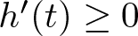 $h'(t)\geq 0$ for
  $t\geq 0$, we have
 \begin{equation}\begin{aligned}
\bar{I}_t-D\bar{I}_{xx}-\sigma L_1
=&\ 2L_2[2N-2N^2(h(t)-x)]h'(t)+4DL_2N^2-\sigma L_1 \\
\geq&\ 4DL_2N^2-\sigma L_1 \geq 0 \quad \text{for }(t,x)\in\Delta_T
\end{aligned}
\end{equation}
\begin{equation}\begin{aligned}
\bar{I}_t-D\bar{I}_{xx}-\sigma L_1
=&\ 2L_2[2N-2N^2(h(t)-x)]h'(t)+4DL_2N^2-\sigma L_1 \\
\geq&\ 4DL_2N^2-\sigma L_1 \geq 0 \quad \text{for }(t,x)\in\Delta_T
\end{aligned}
\end{equation}provided that
 \begin{equation*}
N \gt \left(\frac{\sigma L_1}{4DL_2}\right)^{1/2}.
\end{equation*}
\begin{equation*}
N \gt \left(\frac{\sigma L_1}{4DL_2}\right)^{1/2}.
\end{equation*} Therefore, we can apply the usual comparison principle over  $\Delta_T$ to conclude that
  $I(t,x)\leq \bar{I}(t,x)$ in
  $\Delta_T$ if we choose
 \begin{equation*}
N:=1+\max\left\{\frac{1}{2h_0}, \frac{\|I_0\|_{C^1([-h_0,h_0])}}{L_2},\left(\frac{\sigma L_1}{4DL_2}\right)^{1/2}\right\}.
\end{equation*}
\begin{equation*}
N:=1+\max\left\{\frac{1}{2h_0}, \frac{\|I_0\|_{C^1([-h_0,h_0])}}{L_2},\left(\frac{\sigma L_1}{4DL_2}\right)^{1/2}\right\}.
\end{equation*} Since 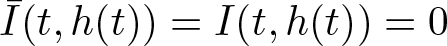 $\bar{I}(t,h(t))=I(t,h(t))=0$, it follows that
 \begin{equation*}
I_x(t,h(t))\geq \bar{I}_x(t,h(t))=-4L_2N\,\text{for }t\in(0,T),
\end{equation*}
\begin{equation*}
I_x(t,h(t))\geq \bar{I}_x(t,h(t))=-4L_2N\,\text{for }t\in(0,T),
\end{equation*}which in turn gives
 \begin{equation*}
h'(t)=-\mu I_x(t,h(t))\leq -\mu\bar{I}_x(t,h(t))\leq 4\mu L_2N\,\text{for }t\in(0,T).
\end{equation*}
\begin{equation*}
h'(t)=-\mu I_x(t,h(t))\leq -\mu\bar{I}_x(t,h(t))\leq 4\mu L_2N\,\text{for }t\in(0,T).
\end{equation*}The proof is thus complete.
Based on the above estimates, we are now in a position to prove that  $(E,I,S)$ is actually a global solution.
Theorem 2.2. The solution  $(E,I,S,g,h)$ given in Theorem 2.1 can be uniquely extended to
  $t\in (0, \infty)$.
Proof. By Theorem 2.1, problem (3) admits a unique solution  $(E,I,S,g,h)$ defined for
  $t\in[0, T_{\max})$ with
  $T_{max}$ the maximal existence time. It remains to show that
  $T_{\max}=\infty$. Assume to the contrary that
  $T_{\max} \lt \infty$. By Lemma 2.1, there exist positive constants
  $L_i, i=1,2,3$, independent of
  $T_{\max}$, such that for
  $t\in [0, T_{\max})$,
 \begin{equation}
\left\{\begin{array}{ll}
0\leq E(t,x),S(t,x)\leq L_1, \ \ \ &-\infty \lt x \lt \infty, \\
0 \lt I(t,x)\leq L_2,\ \ \ \ \ \ & g(t) \lt x \lt h(t), \\
|h(t)|, |g(t)|\leq h_0+ L_3t,\ \ \ 0 \lt -g'(t),h'(t)\leq L_3.
\end{array}\right.
\end{equation}
\begin{equation}
\left\{\begin{array}{ll}
0\leq E(t,x),S(t,x)\leq L_1, \ \ \ &-\infty \lt x \lt \infty, \\
0 \lt I(t,x)\leq L_2,\ \ \ \ \ \ & g(t) \lt x \lt h(t), \\
|h(t)|, |g(t)|\leq h_0+ L_3t,\ \ \ 0 \lt -g'(t),h'(t)\leq L_3.
\end{array}\right.
\end{equation} For any small  $\epsilon \gt 0$, it follows from the proof of Theorem 2.1 that
 \begin{eqnarray*}
&I\in C^{\frac{1+\gamma}{2},1+\gamma}(\Sigma_{T_{max}-\epsilon}), E\in C^{\frac{\gamma}{2},\gamma}(\Sigma_{T_{max}-\epsilon}),\\
& S\in C^{\frac{\gamma}{2},\gamma}([0,T_{max}-\epsilon]\times\mathbb{R})\,\text{and }h,g\in C^{1+\gamma/2}([0, T_{max}-\epsilon]).
\end{eqnarray*}
\begin{eqnarray*}
&I\in C^{\frac{1+\gamma}{2},1+\gamma}(\Sigma_{T_{max}-\epsilon}), E\in C^{\frac{\gamma}{2},\gamma}(\Sigma_{T_{max}-\epsilon}),\\
& S\in C^{\frac{\gamma}{2},\gamma}([0,T_{max}-\epsilon]\times\mathbb{R})\,\text{and }h,g\in C^{1+\gamma/2}([0, T_{max}-\epsilon]).
\end{eqnarray*} By using arguments similar to Step 9 of the proof of Theorem 2.1, for any fixed  $T\in [0,T_{max}-\epsilon)$, we can apply Schauder’s estimate to obtain that
 \begin{equation*}
\|I\|_{C^{1+\frac{\gamma}{2},2+\gamma}(\Sigma_{T_{max}-\epsilon}\backslash\Sigma_T)}\leq C^*,
\end{equation*}
\begin{equation*}
\|I\|_{C^{1+\frac{\gamma}{2},2+\gamma}(\Sigma_{T_{max}-\epsilon}\backslash\Sigma_T)}\leq C^*,
\end{equation*}where  $C^*$ depends on
  $T$,
$T$,  $T_{max}$ and
  $L_i$ for
  $i=1,2,3$, but independent of
  $\epsilon$. By the arbitrariness of small
  $\epsilon \gt 0$, one has
  $\|I(t,\cdot)\|_{C^{2+\gamma}([g(t),h(t)])}\leq C^*$ for all
  $t\in[T,T_{max})$. Then we can repeat the proof of Theorem 2.1 to obtain that there exists
  $\tau \gt 0$, depending on
  $C^*$ and
  $L_i$ for
  $i=1,2,3,$ such that the solution
  $(E,I,S,g,h)$ of (3) can be extended uniquely up to
  $T_{\max}-\tau/2+\tau$. This contradicts the definition of
  $T_{\max}$. The proof is thus complete.
3. Long-time dynamics
In this section, we study the long-time behaviour of  $ (E, I, S, g,h) $. By Lemma 2.1, we see that the free boundary
  $ x = h(t) $ is strictly increasing, while
  $ x = g(t) $ is strictly decreasing with respect to time
  $ t $. Therefore, we have either
  $0 \lt h_\infty-g_\infty \lt \infty$ or
  $h_{\infty}-g_\infty =\infty$, where
 \begin{equation*}h_\infty:=\lim_{t\to\infty} h(t)\in (h_0, \infty],~~ g_\infty:=\lim_{t\to\infty} g(t)\in [-\infty, -h_0).\end{equation*}
We first present some preliminary lemmas, which will be used later.
Lemma 3.1. [Reference Wang and Zhang32, Lemma 4.1] Let  $d,C,\mu,\eta_0$ be some positive constants. If
  $(w,\eta)$ satisfies
 \begin{eqnarray*}
\left\{\begin{array}{ll}
w_t-d w_{xx}\geq -C w, \quad&0 \lt t \lt +\infty,\ 0 \lt x \lt \eta(t),\\
w\geq0, \quad &0 \lt t \lt +\infty,\ x=0,\\
w=0,\ \eta'(t)\geq -\mu w_x,\ \quad &0 \lt t \lt +\infty, x=\eta(t),\\
w(0,x)=w_0(x)\geq,\not\equiv0, \quad& 0 \lt x \lt \eta_0,\\
\eta(0)=\eta_0,
\end{array}\right.
\end{eqnarray*}
\begin{eqnarray*}
\left\{\begin{array}{ll}
w_t-d w_{xx}\geq -C w, \quad&0 \lt t \lt +\infty,\ 0 \lt x \lt \eta(t),\\
w\geq0, \quad &0 \lt t \lt +\infty,\ x=0,\\
w=0,\ \eta'(t)\geq -\mu w_x,\ \quad &0 \lt t \lt +\infty, x=\eta(t),\\
w(0,x)=w_0(x)\geq,\not\equiv0, \quad& 0 \lt x \lt \eta_0,\\
\eta(0)=\eta_0,
\end{array}\right.
\end{eqnarray*}and there exists some constant  $M \gt 0$ such that
 \begin{eqnarray*}
&\lim_{t\rightarrow\infty}\eta(t)=\eta_{\infty} \lt \infty, ~~\lim_{t\rightarrow\infty}\eta'(t)=0,~~\|w(t,\cdot)\|_{C^{1}[0,\eta(t)]}\leq M, \ \forall t \gt 1.
\end{eqnarray*}
\begin{eqnarray*}
&\lim_{t\rightarrow\infty}\eta(t)=\eta_{\infty} \lt \infty, ~~\lim_{t\rightarrow\infty}\eta'(t)=0,~~\|w(t,\cdot)\|_{C^{1}[0,\eta(t)]}\leq M, \ \forall t \gt 1.
\end{eqnarray*}Then
 \begin{eqnarray*}
\lim_{t\rightarrow \infty}\|w(t,\cdot)\|_{C([0,h(t)])}=0.
\end{eqnarray*}
\begin{eqnarray*}
\lim_{t\rightarrow \infty}\|w(t,\cdot)\|_{C([0,h(t)])}=0.
\end{eqnarray*}Lemma 3.2. Let  $(E,I,S,g,h)$ be the solution of (3). Suppose that
  $T\in(0,\infty)$,
  $\bar{g},\bar{h}\in C^{1}([0,T])$,
  $\bar{E},\bar{I}\in C(\bar{G}_{T})\cap C^{1,2}(G_{T})$ with
  $G_{T}=\{(t,x)\in\mathbb{R}^{2}: 0 \lt t\leq T,\, \bar{g}(t) \lt x \lt \bar{h}(t)\}$, and
 \begin{eqnarray*}
\left\{\begin{array}{ll}
\bar{E}_t \geq \beta K \bar{I}-(\sigma+b) \bar{E},\ &0 \lt t\leq T,\ \ \bar{g}(t) \lt x \lt \bar{h}(t),\\
\bar{I}_t\geq D\bar{I}_{xx}+ \sigma \bar{E}-(\alpha+b) \bar{I}, \ &0 \lt t\leq T,\ \ \bar{g}(t) \lt x \lt \bar{h}(t),\\
\bar{I}(t, \bar{g}(t))=\bar{I}(t, \bar{h}(t))=0,\ &0 \lt t\leq T,\\
\bar{h}'(t)\geq - \bar{I}_x(t,\bar{h}(t)), \ &0 \lt t\leq T,\\
\bar{g}'(t)\leq -\bar{I}_x(t,\bar{g}(t)), \ &0 \lt t\leq T,\\
\bar{E}(0,x)\geq E_0(x), \bar{I}(0,x)\geq I_0(x),\ &-h_0\leq x\leq h_0,\\
\bar{h}(0)\geq h_0, \bar{g}(0)\leq-h_0.
\end{array}\right.
\end{eqnarray*}
\begin{eqnarray*}
\left\{\begin{array}{ll}
\bar{E}_t \geq \beta K \bar{I}-(\sigma+b) \bar{E},\ &0 \lt t\leq T,\ \ \bar{g}(t) \lt x \lt \bar{h}(t),\\
\bar{I}_t\geq D\bar{I}_{xx}+ \sigma \bar{E}-(\alpha+b) \bar{I}, \ &0 \lt t\leq T,\ \ \bar{g}(t) \lt x \lt \bar{h}(t),\\
\bar{I}(t, \bar{g}(t))=\bar{I}(t, \bar{h}(t))=0,\ &0 \lt t\leq T,\\
\bar{h}'(t)\geq - \bar{I}_x(t,\bar{h}(t)), \ &0 \lt t\leq T,\\
\bar{g}'(t)\leq -\bar{I}_x(t,\bar{g}(t)), \ &0 \lt t\leq T,\\
\bar{E}(0,x)\geq E_0(x), \bar{I}(0,x)\geq I_0(x),\ &-h_0\leq x\leq h_0,\\
\bar{h}(0)\geq h_0, \bar{g}(0)\leq-h_0.
\end{array}\right.
\end{eqnarray*}Then
 \begin{eqnarray*}
&[g(t),h(t)]\subseteq [\bar{g}(t),\bar{h}(t)] \text{for }t\in(0,T], \\
&E(t,x)\leq \bar{E}(t,x),\ I(t,x)\leq \bar{I}(t,x) \text{for }t\in (0, T]\text{and } g(t) \lt x \lt h(t).
\end{eqnarray*}
\begin{eqnarray*}
&[g(t),h(t)]\subseteq [\bar{g}(t),\bar{h}(t)] \text{for }t\in(0,T], \\
&E(t,x)\leq \bar{E}(t,x),\ I(t,x)\leq \bar{I}(t,x) \text{for }t\in (0, T]\text{and } g(t) \lt x \lt h(t).
\end{eqnarray*}Proof. By Lemma 2.1 and (3), we know that  $(E,I)$ satisfies
 \begin{align}
\begin{cases}
E_{t}\leq \beta K I-(\sigma+b)E, & t \gt 0, \ g(t) \lt x \lt h(t), \\
I_{t}\leq D I_{xx}+\sigma E-(\alpha+b) I, & t \gt 0, \ g(t) \lt x \lt h(t).
\end{cases}
\end{align}
\begin{align}
\begin{cases}
E_{t}\leq \beta K I-(\sigma+b)E, & t \gt 0, \ g(t) \lt x \lt h(t), \\
I_{t}\leq D I_{xx}+\sigma E-(\alpha+b) I, & t \gt 0, \ g(t) \lt x \lt h(t).
\end{cases}
\end{align}The rest of the proof is similar to that of [Reference Wang and Du34, Lemma 2.3], and is therefore omitted.
Lemma 3.3. If  $h_\infty-g_\infty \lt \infty$, then there exists a constant
  $M \gt 0$, such that the solution
  $(E,I,S,g,h)$ of (3) satisfies
 \begin{eqnarray*}
&\|I(t,\cdot)\|_{C^1[g(t),h(t)]}\leq M\,\mbox{for } t \gt 1, \ \ \|g'\|_{C^{\frac{\alpha}{2}}([1,+\infty))}+\|h'\|_{C^{\frac{\alpha}{2}}([1,+\infty))}\leq M,\\
&\displaystyle\lim\limits_{t\to\infty}g'(t)=\displaystyle\lim\limits_{t\to\infty}h'(t)=0.
\end{eqnarray*}
\begin{eqnarray*}
&\|I(t,\cdot)\|_{C^1[g(t),h(t)]}\leq M\,\mbox{for } t \gt 1, \ \ \|g'\|_{C^{\frac{\alpha}{2}}([1,+\infty))}+\|h'\|_{C^{\frac{\alpha}{2}}([1,+\infty))}\leq M,\\
&\displaystyle\lim\limits_{t\to\infty}g'(t)=\displaystyle\lim\limits_{t\to\infty}h'(t)=0.
\end{eqnarray*}Proof. Since  $-g'(t),h'(t) \gt 0$, the inequality
  $h_\infty-g_\infty \lt \infty$ implies that
  $-\infty \lt h_\infty,g_\infty \lt \infty$. Define
 \begin{equation*}
y:=\frac{g_\infty(h(t)-x)+h_\infty(x-g(t))}{h(t)-g(t)}
\end{equation*}
\begin{equation*}
y:=\frac{g_\infty(h(t)-x)+h_\infty(x-g(t))}{h(t)-g(t)}
\end{equation*}and
 \begin{equation*}
z_1(t,y):=E(t,x),~z_2(t,y):=I(t,x)\,\text{and }z_3(t,y):=S(t,x)\,\text{for }x\in[g(t),h(t)].
\end{equation*}
\begin{equation*}
z_1(t,y):=E(t,x),~z_2(t,y):=I(t,x)\,\text{and }z_3(t,y):=S(t,x)\,\text{for }x\in[g(t),h(t)].
\end{equation*} Then,  $z_2$ solves
 \begin{equation}
\begin{cases}
z_{2t}-d\left[\frac{h_\infty-g_\infty}{h(t)-g(t)}\right]^2 z_{2yy}&\\
+\frac{h'(t)g_\infty-g'(t)h_\infty-[h'(t)-g'(t)]y}{h(t)-g(t)}z_{2y}=f_3(z_1,z_2,z_3),&t \gt 0,y\in[g_\infty,h_\infty],\\
z_2(t,g_\infty)=z_2(t,h_\infty)=0,& t \gt 0,\\
h'(t)=-\frac{\mu(h_\infty-g_\infty)}{h(t)-g(t)}z_{2y}(t,h_\infty),&t \gt 0,\\
g'(t)=-\frac{\mu(h_\infty-g_\infty)}{h(t)-g(t)}z_{2y}(t,g_\infty),&t \gt 0,\\
z_2(0,y)=I_0\left[\frac{2h_0y-h_0(g_\infty+h_\infty)}{h_\infty-g_\infty}\right], &y\in[g_\infty,h_\infty].
\end{cases}
\end{equation}
\begin{equation}
\begin{cases}
z_{2t}-d\left[\frac{h_\infty-g_\infty}{h(t)-g(t)}\right]^2 z_{2yy}&\\
+\frac{h'(t)g_\infty-g'(t)h_\infty-[h'(t)-g'(t)]y}{h(t)-g(t)}z_{2y}=f_3(z_1,z_2,z_3),&t \gt 0,y\in[g_\infty,h_\infty],\\
z_2(t,g_\infty)=z_2(t,h_\infty)=0,& t \gt 0,\\
h'(t)=-\frac{\mu(h_\infty-g_\infty)}{h(t)-g(t)}z_{2y}(t,h_\infty),&t \gt 0,\\
g'(t)=-\frac{\mu(h_\infty-g_\infty)}{h(t)-g(t)}z_{2y}(t,g_\infty),&t \gt 0,\\
z_2(0,y)=I_0\left[\frac{2h_0y-h_0(g_\infty+h_\infty)}{h_\infty-g_\infty}\right], &y\in[g_\infty,h_\infty].
\end{cases}
\end{equation} By the estimates in Lemma 2.1, we can apply the standard  $L^p$ theory and the Sobolev embedding theorem to (2) to deduce that
 \begin{equation*}
\|z_2\|_{C^{(1+\alpha)/2,1+\alpha}([m,m+1]\times[g_\infty,h_\infty])}\leq C_1\,\text{for any }m\geq 1,
\end{equation*}
\begin{equation*}
\|z_2\|_{C^{(1+\alpha)/2,1+\alpha}([m,m+1]\times[g_\infty,h_\infty])}\leq C_1\,\text{for any }m\geq 1,
\end{equation*}where  $C_1 \gt 0$ is a constant independent of
  $m$, which implies that
 \begin{equation*}\|g'\|_{C^{\frac{\alpha}{2}}([m,m+1])}+\|h'\|_{C^{\frac{\alpha}{2}}([m,m+1])}\leq C_2\end{equation*}
with  $C_2$ depending on
  $C_1$,
  $\mu$,
  $h_0$,
  $g^*$,
  $h^*$,
  $g_\infty$ and
  $h_\infty$. We now claim that
  $g'(t)\to 0$ and
  $h'(t)\to 0$ as
  $t\to\infty$. Without loss of generality, suppose on the contrary that there exist
  $\{t_n\}$ and
  $a \gt 0$ such that
  $t_n\to\infty$ and
  $h'(t_n)\to a$ as
  $n\to\infty$. Then there exists a constant
  $\sigma \gt 0$ such that
  $h'(t) \gt a/2$ for
 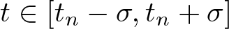 $t\in[t_n-\sigma,t_n+\sigma]$ and all large
  $n$, which yields
  $h_\infty=\infty$. This is a contradiction.
Recall that the rabid foxes is said to exhibit spreading if 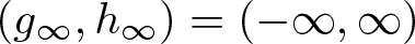 $(g_\infty,h_\infty)=(-\infty,\infty)$ and
 \begin{equation*}
\limsup_{t \to \infty}I(t, x) \gt 0\,\text{locally uniformly in } x\in\mathbb{R},
\end{equation*}
\begin{equation*}
\limsup_{t \to \infty}I(t, x) \gt 0\,\text{locally uniformly in } x\in\mathbb{R},
\end{equation*}indicating that the range of rabid foxes spread to the entire space, with the density of the rabid foxes persisting weakly. One says that vanishing occurs if 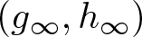 $(g_\infty, h_\infty)$ is a finite interval and
 \begin{equation*}
\lim_{t \to \infty} \| I(t, \cdot) \|_{C([g(t), h(t)])} = 0,
\end{equation*}
\begin{equation*}
\lim_{t \to \infty} \| I(t, \cdot) \|_{C([g(t), h(t)])} = 0,
\end{equation*}in which case, the rabid fox population remains confined to a bounded region and eventually dies out.
3.1. The case of vanishing
Theorem 3.1. Let  $(E,I,S,g,h)$ be a solution of (3). If
  $h_{\infty}-g_{\infty} \lt \infty$, then
 \begin{equation*}\begin{cases}
\displaystyle\lim_{t\rightarrow\infty}\|E(t,\cdot)\|_{C([g(t),h(t)])}=\displaystyle\lim_{t\rightarrow\infty}\|I(t,\cdot)\|_{C([g(t),h(t)])}=0. \\
\displaystyle\lim_{t\rightarrow\infty}S(t,x)=K\ \ \textit{uniformly on any compact subset of } \mathbb{R}.
\end{cases}\end{equation*}
\begin{equation*}\begin{cases}
\displaystyle\lim_{t\rightarrow\infty}\|E(t,\cdot)\|_{C([g(t),h(t)])}=\displaystyle\lim_{t\rightarrow\infty}\|I(t,\cdot)\|_{C([g(t),h(t)])}=0. \\
\displaystyle\lim_{t\rightarrow\infty}S(t,x)=K\ \ \textit{uniformly on any compact subset of } \mathbb{R}.
\end{cases}\end{equation*}Proof. Since  $E$,
$E$,  $I$ and
  $S$ are nonnegative and bounded, by virtue of Lemma 3.3, we may apply Lemma 3.1 to the equations satisfied by
  $I$ to obtain that
 \begin{eqnarray*}
\displaystyle\lim_{t\rightarrow\infty}\|I(t,\cdot)\|_{C([g(t),h(t)])}=0.
\end{eqnarray*}
\begin{eqnarray*}
\displaystyle\lim_{t\rightarrow\infty}\|I(t,\cdot)\|_{C([g(t),h(t)])}=0.
\end{eqnarray*} Hence, for any given small  $\epsilon\in(0,1)$, there exists
  $T \gt 0$ such that
 \begin{equation*}\|I(t,\cdot)\|_{C([g(t),h(t)])}\leq \epsilon\,\text{for }t\geq T.\end{equation*}
Combining this with (3) and Lemma 2.1, we obtain
 \begin{equation*}
\begin{cases}
E_t\leq \beta K\epsilon-\sigma E, &t\geq T,x\in\mathbb{R},\\
E(T,x)\leq L_1, & x\in\mathbb{R}.
\end{cases}
\end{equation*}
\begin{equation*}
\begin{cases}
E_t\leq \beta K\epsilon-\sigma E, &t\geq T,x\in\mathbb{R},\\
E(T,x)\leq L_1, & x\in\mathbb{R}.
\end{cases}
\end{equation*}It follows immediately that
 \begin{equation*}
E(t,x)\leq (L_1-\frac{\beta K\epsilon}{\sigma})e^{-\sigma (t-T)}+\frac{\beta K\epsilon}{\sigma}\,\text{for }t\geq T,x\in\mathbb{R}.
\end{equation*}
\begin{equation*}
E(t,x)\leq (L_1-\frac{\beta K\epsilon}{\sigma})e^{-\sigma (t-T)}+\frac{\beta K\epsilon}{\sigma}\,\text{for }t\geq T,x\in\mathbb{R}.
\end{equation*} Letting  $t\to\infty$ and then
  $\epsilon\to 0$, we obtain
 \begin{equation*}
\limsup_{t\to\infty} E(t,x)\leq 0\,\text{for } x\in[g(t),h(t)]\subset \mathbb{R}.
\end{equation*}
\begin{equation*}
\limsup_{t\to\infty} E(t,x)\leq 0\,\text{for } x\in[g(t),h(t)]\subset \mathbb{R}.
\end{equation*} Since  $E$ is nonnegative, we get
 \begin{eqnarray*}
\displaystyle\lim_{t\rightarrow\infty}\|E(t,\cdot)\|_{C([g(t),h(t)])}=0.
\end{eqnarray*}
\begin{eqnarray*}
\displaystyle\lim_{t\rightarrow\infty}\|E(t,\cdot)\|_{C([g(t),h(t)])}=0.
\end{eqnarray*} Consequently, for any small  $\delta\in(0,1)$ and
  $l \gt 0$, there exists
  $T \gt 0$ such that
 \begin{eqnarray*}
E(t,x)\leq \delta,\ I(t,x)\leq \delta\,\text{for } t\geq T, x\in[-l,l].
\end{eqnarray*}
\begin{eqnarray*}
E(t,x)\leq \delta,\ I(t,x)\leq \delta\,\text{for } t\geq T, x\in[-l,l].
\end{eqnarray*}By (3), we have
 \begin{align*}
&S_{t}\geq (a-b)S\left(1-\displaystyle\frac{2\delta}{K}-\displaystyle\frac{\delta\beta}{a-b}-\frac SK\right) \text{for } t\geq T,x\in[-l,l]; \\
&\quad S(T,x)\geq \min_{x\in[-l,l]}S(T,x) \gt 0.
\end{align*}
\begin{align*}
&S_{t}\geq (a-b)S\left(1-\displaystyle\frac{2\delta}{K}-\displaystyle\frac{\delta\beta}{a-b}-\frac SK\right) \text{for } t\geq T,x\in[-l,l]; \\
&\quad S(T,x)\geq \min_{x\in[-l,l]}S(T,x) \gt 0.
\end{align*}Consider the following ODE problem:
 \begin{eqnarray*}
\left\{\begin{array}{ll}
\underline{S}_t=(a-b)\underline{S}\left(1-\displaystyle\frac{2\delta}{K}-\displaystyle\frac{\delta\beta}{a-b}-\frac{\underline{S}}K\right),\ \ t \gt T,\\
\underline{S}(T)=\min_{x\in[-L,L]}S(T,x) \gt 0.
\end{array}\right.
\end{eqnarray*}
\begin{eqnarray*}
\left\{\begin{array}{ll}
\underline{S}_t=(a-b)\underline{S}\left(1-\displaystyle\frac{2\delta}{K}-\displaystyle\frac{\delta\beta}{a-b}-\frac{\underline{S}}K\right),\ \ t \gt T,\\
\underline{S}(T)=\min_{x\in[-L,L]}S(T,x) \gt 0.
\end{array}\right.
\end{eqnarray*}It follows from the comparison principle that
 \begin{eqnarray*}
0\leq \underline{S}(t,x)\leq S(t,x)\,\text{for } t \gt T, -l \lt x \lt l.
\end{eqnarray*}
\begin{eqnarray*}
0\leq \underline{S}(t,x)\leq S(t,x)\,\text{for } t \gt T, -l \lt x \lt l.
\end{eqnarray*}Hence,
 \begin{eqnarray*}
\liminf_{t\rightarrow\infty}\min_{x\in[-L,L]} S(t,x)\geq \lim_{t\rightarrow \infty}\underline{S}(t)=K-2\delta-\displaystyle\frac{\delta\beta K}{a-b}.
\end{eqnarray*}
\begin{eqnarray*}
\liminf_{t\rightarrow\infty}\min_{x\in[-L,L]} S(t,x)\geq \lim_{t\rightarrow \infty}\underline{S}(t)=K-2\delta-\displaystyle\frac{\delta\beta K}{a-b}.
\end{eqnarray*} Since  $\delta \gt 0$ can be chosen arbitrarily small, it follows that
 \begin{equation}
\liminf_{t\rightarrow\infty}\min_{x\in[-L,L]}S(t,x)\geq K.
\end{equation}
\begin{equation}
\liminf_{t\rightarrow\infty}\min_{x\in[-L,L]}S(t,x)\geq K.
\end{equation} This, together with  $S(t,x)\leq K$, yields the desired result. The proof is thus completed.
Define
 \begin{equation}
\mathcal{R}_0^*:=\displaystyle\frac{\beta\sigma K}{(\alpha+b)(\sigma+b)}.
\end{equation}
\begin{equation}
\mathcal{R}_0^*:=\displaystyle\frac{\beta\sigma K}{(\alpha+b)(\sigma+b)}.
\end{equation} Note that  $a \gt b$ implies
  $\mathcal{R}_0^* \gt \mathcal R_0$, where
  $\mathcal R_0 $ is given in (2). The following result shows that if
 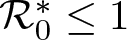 $\mathcal{R}_0^*\leq 1$, the rabid foxes cannot spread to the entire space
  $\mathbb{R}$ and must eventually vanish.
Theorem 3.2. Let 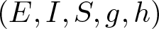 $(E,I,S,g,h)$ be the solution of (3). If
  $\mathcal{R}_0^*\leq1$, then
 \begin{eqnarray*}
h_{\infty}-g_{\infty}\leq \displaystyle\frac{\mu}{D} \int^{h_0}_{-h_0}\left[ I_0(x)+\frac{\sigma}{\sigma+b}E_0(x)\right]dx+2 h_0,
\end{eqnarray*}
\begin{eqnarray*}
h_{\infty}-g_{\infty}\leq \displaystyle\frac{\mu}{D} \int^{h_0}_{-h_0}\left[ I_0(x)+\frac{\sigma}{\sigma+b}E_0(x)\right]dx+2 h_0,
\end{eqnarray*}and vanishing occurs.
Proof. By (3) and Lemma 2.1 , we have
 \begin{eqnarray*}
\begin{cases}
E_{t}\leq \beta K I-(\sigma+b)E, &t \gt 0, \ g(t) \lt x \lt h(t),\\
I_{t}\leq D I_{xx}+\sigma E-(\alpha+b) I, &t \gt 0, \ g(t) \lt x \lt h(t).
\end{cases}
\end{eqnarray*}
\begin{eqnarray*}
\begin{cases}
E_{t}\leq \beta K I-(\sigma+b)E, &t \gt 0, \ g(t) \lt x \lt h(t),\\
I_{t}\leq D I_{xx}+\sigma E-(\alpha+b) I, &t \gt 0, \ g(t) \lt x \lt h(t).
\end{cases}
\end{eqnarray*}Denote
 \begin{equation*}U(t):=\int^{h(t)}_{g(t)}\left[ I(t,x)+\frac{\sigma}{\sigma+b}E(t,x)\right]dx.\end{equation*}
 Then 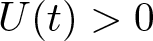 $U(t) \gt 0$ for
  $t\geq 0$ and
 \begin{equation*}\begin{aligned}
\displaystyle U'(t)
&= \displaystyle h'(t)[ I(t,h(t))+\frac{\sigma}{\sigma+b} E(t,h(t))]- g'(t)[ I(t,g(t))+\frac{\sigma}{\sigma+b} E(t,g(t))]\displaystyle\nonumber\\
&\ \ \ \ +\int^{h(t)}_{g(t)}[ I_t(t,x)+\frac{\sigma}{\sigma+b} E_{t}(t,x)]dx\displaystyle\nonumber\\
&\leq \displaystyle\int^{h(t)}_{g(t)}[D I_{xx} +\sigma E-(\alpha+b) I]dx+\int^{ h(t)}_{ g(t)}[\frac{\sigma }{\sigma+b} \beta K I-\sigma E]dx \nonumber\\
&\leq -\frac{D}{\mu} h'(t)+\frac{D}{\mu}g'(t)+\int^{h(t)}_{g(t)}[\frac{\beta \sigma K}{\sigma+b}-(\alpha+b)] Idx.
\end{aligned}
\end{equation*}
\begin{equation*}\begin{aligned}
\displaystyle U'(t)
&= \displaystyle h'(t)[ I(t,h(t))+\frac{\sigma}{\sigma+b} E(t,h(t))]- g'(t)[ I(t,g(t))+\frac{\sigma}{\sigma+b} E(t,g(t))]\displaystyle\nonumber\\
&\ \ \ \ +\int^{h(t)}_{g(t)}[ I_t(t,x)+\frac{\sigma}{\sigma+b} E_{t}(t,x)]dx\displaystyle\nonumber\\
&\leq \displaystyle\int^{h(t)}_{g(t)}[D I_{xx} +\sigma E-(\alpha+b) I]dx+\int^{ h(t)}_{ g(t)}[\frac{\sigma }{\sigma+b} \beta K I-\sigma E]dx \nonumber\\
&\leq -\frac{D}{\mu} h'(t)+\frac{D}{\mu}g'(t)+\int^{h(t)}_{g(t)}[\frac{\beta \sigma K}{\sigma+b}-(\alpha+b)] Idx.
\end{aligned}
\end{equation*} Since 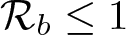 $\mathcal{R}_b\leq 1$, it follows that
 \begin{equation}
\displaystyle U'(t)\leq -\frac{D}{\mu} h'(t)+\frac{D}{\mu}g'(t).
\end{equation}
\begin{equation}
\displaystyle U'(t)\leq -\frac{D}{\mu} h'(t)+\frac{D}{\mu}g'(t).
\end{equation} Integrating (5) from  $0$ to
  $t$, we obtain
 \begin{eqnarray*}
U(t)\leq U(0)-\displaystyle\frac{D}{\mu}( h(t)- g(t))+\displaystyle\frac{2D}{\mu} h_0\,\mbox{for } t \gt 0,
\end{eqnarray*}
\begin{eqnarray*}
U(t)\leq U(0)-\displaystyle\frac{D}{\mu}( h(t)- g(t))+\displaystyle\frac{2D}{\mu} h_0\,\mbox{for } t \gt 0,
\end{eqnarray*}which implies
 \begin{eqnarray*}
h(t)- g(t)\leq \displaystyle\frac{\mu}{D} U(0)+2 h_0\ \mbox{for all} \ t \gt 0.
\end{eqnarray*}
\begin{eqnarray*}
h(t)- g(t)\leq \displaystyle\frac{\mu}{D} U(0)+2 h_0\ \mbox{for all} \ t \gt 0.
\end{eqnarray*} Hence  $h_{\infty}-g_{\infty} \lt \infty$, and by Lemma 3.1, vanishing happens.
If  $\mathcal{R}_0^* \gt 1$, vanishing can also occur, and to find out when, we need the following eigenvalue problem. For any given
  $l \gt 0$, we consider the problem:
 \begin{equation}
\left\{\begin{array}{ll}
(\sigma+b)\phi_1-\beta K \phi_2=\lambda \phi_1,\ \ &-l \lt x \lt l,\\
-D \phi_2'' -\sigma \phi_1+(\alpha+b)\phi_2=\lambda \phi_2,\ &-l \lt x \lt l,\\
\phi_2(-l_1)=\phi_2(l_2)=0.
\end{array}\right.
\end{equation}
\begin{equation}
\left\{\begin{array}{ll}
(\sigma+b)\phi_1-\beta K \phi_2=\lambda \phi_1,\ \ &-l \lt x \lt l,\\
-D \phi_2'' -\sigma \phi_1+(\alpha+b)\phi_2=\lambda \phi_2,\ &-l \lt x \lt l,\\
\phi_2(-l_1)=\phi_2(l_2)=0.
\end{array}\right.
\end{equation} By expressing  $\phi_1$ in terms of
  $\phi_2$ using the first equation and substituting into the second, (6) is reduced to the following eigenvalue problem:
 \begin{eqnarray*}
\left\{\begin{array}{ll}
-D \phi_2'' +(\alpha+b)\phi_2-\displaystyle\frac{\sigma \beta K}{\sigma+b-\lambda}\phi_2 =\lambda \phi_2,\ &-l \lt x \lt l,\\
\phi_2(-l)=\phi_2(l)=0,
\end{array}\right.
\end{eqnarray*}
\begin{eqnarray*}
\left\{\begin{array}{ll}
-D \phi_2'' +(\alpha+b)\phi_2-\displaystyle\frac{\sigma \beta K}{\sigma+b-\lambda}\phi_2 =\lambda \phi_2,\ &-l \lt x \lt l,\\
\phi_2(-l)=\phi_2(l)=0,
\end{array}\right.
\end{eqnarray*}Direct calculation shows that the above problem admits two principal eigenvalues
 \begin{equation*}
\lambda^{\pm}:=\lambda^{\pm}(l)=\frac{\sigma+b+\alpha+b+\eta_1\pm\sqrt{[\sigma+b-(\alpha+b+\eta_1)]^2+4\sigma\beta K}}{2}
\end{equation*}
\begin{equation*}
\lambda^{\pm}:=\lambda^{\pm}(l)=\frac{\sigma+b+\alpha+b+\eta_1\pm\sqrt{[\sigma+b-(\alpha+b+\eta_1)]^2+4\sigma\beta K}}{2}
\end{equation*}associated with the same eigenfunction  $\Phi^*=\cos(\displaystyle\frac{1}{2l}\pi x)$, where
  $(\eta_1,\Phi^*):=(\frac{D\pi^2}{4l^2},\Phi^*(l))$ is the principal eigenvalue and eigenfunction of
 \begin{equation}
-D\Phi_{xx}=\eta \Phi \ \ {\rm in}\ (-l,l),\ \ \Phi(\pm l)=0.
\end{equation}
\begin{equation}
-D\Phi_{xx}=\eta \Phi \ \ {\rm in}\ (-l,l),\ \ \Phi(\pm l)=0.
\end{equation} Clearly,  $\lambda^+ \gt \sigma+b \gt \lambda^-$. Therefore,
  $\lambda^-$ is the unique principal eigenvalue of (6) associated with positive eigenfunction
 \begin{equation*}(\phi_1^*,\phi_2^*)=(\displaystyle\frac{\beta K}{\sigma+b-\lambda^-}\Phi^*,\Phi^*).\end{equation*}
 ( $\lambda^+$ gives the eigenpair
 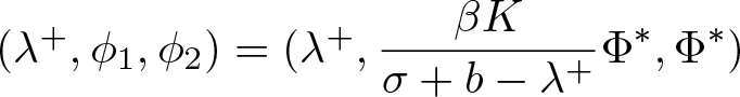 $(\lambda^+, \phi_1,\phi_2)=(\lambda^+, \displaystyle\frac{\beta K}{\sigma+b-\lambda^+}\Phi^*,\Phi^*)$ of (6) with
  $\phi_1 \lt 0$, so not meeting the requirement as a principal eigenvalue.)
Define
 \begin{eqnarray*}
R(l):=\displaystyle\frac{\sigma\beta K}{(\eta_1+\alpha+b)(\sigma+b)}=\displaystyle\frac{\sigma\beta K}{\left(D\left(\displaystyle\frac{\pi}{2l}\right)^2+\alpha+b\right)\left(\sigma+b\right)}.
\end{eqnarray*}
\begin{eqnarray*}
R(l):=\displaystyle\frac{\sigma\beta K}{(\eta_1+\alpha+b)(\sigma+b)}=\displaystyle\frac{\sigma\beta K}{\left(D\left(\displaystyle\frac{\pi}{2l}\right)^2+\alpha+b\right)\left(\sigma+b\right)}.
\end{eqnarray*} It is easy to see that  $R(l)=1$ if and only if
  $\lambda^-=0$. Furthermore,
 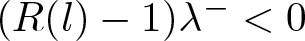 $(R(l)-1)\lambda^- \lt 0$ for
 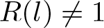 $R(l)\neq 1$, and
  $R(l)$ is strictly decreasing in
  $D$ and strictly increasing in
  $l$. Moreover,
 \begin{eqnarray*}
\lim_{D\rightarrow +\infty}R(l)=\lim_{l\rightarrow 0}R(l)=0,\ \ \lim_{D\rightarrow 0}R(l)=\lim_{l\rightarrow +\infty}R(l)=\displaystyle\frac{\beta \sigma K}{(\alpha+b)(\sigma+b)}=\mathcal{R}_0^*.
\end{eqnarray*}
\begin{eqnarray*}
\lim_{D\rightarrow +\infty}R(l)=\lim_{l\rightarrow 0}R(l)=0,\ \ \lim_{D\rightarrow 0}R(l)=\lim_{l\rightarrow +\infty}R(l)=\displaystyle\frac{\beta \sigma K}{(\alpha+b)(\sigma+b)}=\mathcal{R}_0^*.
\end{eqnarray*} Therefore, when  $\mathcal{R}_0^* \gt 1$, there exists a unique
 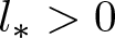 $l_* \gt 0$ such that
 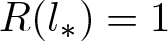 $R(l_*)=1$, and
 \begin{equation}
l_*:=\displaystyle\frac{\pi}{2}\sqrt{\frac{D(\sigma+b)}{\sigma \beta K-(\alpha+b)(\sigma+b)}}.
\end{equation}
\begin{equation}
l_*:=\displaystyle\frac{\pi}{2}\sqrt{\frac{D(\sigma+b)}{\sigma \beta K-(\alpha+b)(\sigma+b)}}.
\end{equation}Theorem 3.3. Let  $(E,I,S,g,h)$ be the solution of (3). If
  $\mathcal{R}_0^* \gt 1$ and
  $h_0 \lt l_*$, then there exists
  $\mu_0 \gt 0$ depending on
  $(E_0,I_0,S_0)$ such that vanishing happens if
  $0 \lt \mu\leq \mu_0.$
Proof. By Lemma 2.1, we know that  $0\leq S(t,x) \lt K$ and
  $E(t,x),I(t,x)\geq 0$. Hence,
  $(E,I)$ satisfies
 \begin{equation}
\left\{\begin{array}{ll}
E_{t}\leq \beta K I -(\sigma+b) E,\ \ &t \gt 0, \ g(t) \lt x \lt h(t),\\
I_{t}=D I_{xx}+\sigma E-(\alpha+b) I ,\ \ &t \gt 0, \ g(t) \lt x \lt h(t)\\
E(t,g(t))=E(t,h(t))=0,\ &t \gt 0, \\
I(t,g(t))=I(t,h(t))=0,\ &t \gt 0,\\
h'(t)=-\mu I_{x}(t,h(t)) , \ &t \gt 0,\\
g'(t)=-\mu I_{x}(t,g(t)), \ &t \gt 0,\\
E(0,x)=E_0(x),\, I(0,x)=I_0(x), \ \ &-h_0\leq x \leq h_0,\\
h(0)=h_0,\,g(0)=-h_0. &
\end{array}\right.
\end{equation}
\begin{equation}
\left\{\begin{array}{ll}
E_{t}\leq \beta K I -(\sigma+b) E,\ \ &t \gt 0, \ g(t) \lt x \lt h(t),\\
I_{t}=D I_{xx}+\sigma E-(\alpha+b) I ,\ \ &t \gt 0, \ g(t) \lt x \lt h(t)\\
E(t,g(t))=E(t,h(t))=0,\ &t \gt 0, \\
I(t,g(t))=I(t,h(t))=0,\ &t \gt 0,\\
h'(t)=-\mu I_{x}(t,h(t)) , \ &t \gt 0,\\
g'(t)=-\mu I_{x}(t,g(t)), \ &t \gt 0,\\
E(0,x)=E_0(x),\, I(0,x)=I_0(x), \ \ &-h_0\leq x \leq h_0,\\
h(0)=h_0,\,g(0)=-h_0. &
\end{array}\right.
\end{equation} Since  $h_0 \lt l_*$, we have
  $R(h_0) \lt 1$, and thus the principal eigenvalue
  $\lambda_0:=\lambda^-$ of (6) with
  $l=h_0$ is positive, with corresponding eigenfunction
 \begin{equation*}(\phi(x),\psi(x)):=\Big(\frac{\beta K}{\sigma+b-\lambda_0}\cos(\frac\pi{2h_0}x),\cos(\frac\pi{2h_0}x)\Big)\end{equation*}
Define
 \begin{equation*}
\begin{cases}
\eta(t):=h_0(1+\delta-\delta e^{-\delta t})\,\text{for }t\geq 0,\\
\bar{E}(t,x):=\displaystyle Me^{-\delta t}\phi\left(x h_0/\eta(t)\right)\text{for } t\geq 0,\ -\eta(t)\leq x\leq \eta(t),\\
\bar{I}(t,x):=Me^{-\delta t}\psi\left(x h_0/\eta(t)\right) \text{for }t\geq 0, -\eta(t)\leq x\leq \eta(t)
\end{cases}
\end{equation*}
\begin{equation*}
\begin{cases}
\eta(t):=h_0(1+\delta-\delta e^{-\delta t})\,\text{for }t\geq 0,\\
\bar{E}(t,x):=\displaystyle Me^{-\delta t}\phi\left(x h_0/\eta(t)\right)\text{for } t\geq 0,\ -\eta(t)\leq x\leq \eta(t),\\
\bar{I}(t,x):=Me^{-\delta t}\psi\left(x h_0/\eta(t)\right) \text{for }t\geq 0, -\eta(t)\leq x\leq \eta(t)
\end{cases}
\end{equation*}with the constants  $\delta \gt 0$ and
  $M \gt 0$ to be determined later. We show that
  $(E,I,\eta,-\eta)$ forms an upper solution of (9).
Clearly,  $\eta(0)=h_0$ and
 \begin{eqnarray*}
&\bar{E}(t,\eta(t))=\bar{E}(t,-\eta(t))=0, \bar{I}(t,\eta(t))= \bar{I}(t,-\eta(t))=0\,\text{for }t \gt 0,\\
&\bar{E}(0,x)=M\phi(x) \gt 0, \bar{I}(0,x)=M\psi(x) \gt 0 \,\text{for } x\in(-h_0,h_0).
\end{eqnarray*}
\begin{eqnarray*}
&\bar{E}(t,\eta(t))=\bar{E}(t,-\eta(t))=0, \bar{I}(t,\eta(t))= \bar{I}(t,-\eta(t))=0\,\text{for }t \gt 0,\\
&\bar{E}(0,x)=M\phi(x) \gt 0, \bar{I}(0,x)=M\psi(x) \gt 0 \,\text{for } x\in(-h_0,h_0).
\end{eqnarray*} Since  $\mp\psi'(\pm h_0)=\frac{\pi}{2h_0} \gt 0$, in view of (4) we can choose
  $M \gt 0$ large enough such that
 \begin{eqnarray*}
\bar{E}(0,x)\geq E_0(x),~ \bar{I}(0,x)\geq I_0(x) \, \text{for } x\in[-h_0,h_0].
\end{eqnarray*}
\begin{eqnarray*}
\bar{E}(0,x)\geq E_0(x),~ \bar{I}(0,x)\geq I_0(x) \, \text{for } x\in[-h_0,h_0].
\end{eqnarray*}By direct calculations, one has
 \begin{align*}
& h_0\leq \eta(t)\leq h_0(1+\delta),~\eta'=h_0\delta^2e^{-\delta t} \gt 0\,\text{for }t\in(0,T],\\
&\bar{E}_t=-\delta Me^{-\delta t}\phi- \displaystyle\frac{M h_0}{\eta^2}x\phi'\eta'e^{-\delta t}\geq -\delta Me^{-\delta t}\phi,\\
& \displaystyle\bar{I}_t=-\delta Me^{-\delta t}\psi- \displaystyle\frac{M h_0}{\eta^2}x\psi'\eta'e^{-\delta t}\geq -\delta Me^{-\delta t}\psi,\\
&\bar{I}_{x}=\frac{h_0}{\eta} Me^{-\delta t}\psi',~ \bar{I}_{xx}=\frac{h_0^2}{\eta^2} Me^{-\delta t}\psi''=-\frac{h_0^2}{\eta^2}Me^{-\delta t}\psi.
\end{align*}
\begin{align*}
& h_0\leq \eta(t)\leq h_0(1+\delta),~\eta'=h_0\delta^2e^{-\delta t} \gt 0\,\text{for }t\in(0,T],\\
&\bar{E}_t=-\delta Me^{-\delta t}\phi- \displaystyle\frac{M h_0}{\eta^2}x\phi'\eta'e^{-\delta t}\geq -\delta Me^{-\delta t}\phi,\\
& \displaystyle\bar{I}_t=-\delta Me^{-\delta t}\psi- \displaystyle\frac{M h_0}{\eta^2}x\psi'\eta'e^{-\delta t}\geq -\delta Me^{-\delta t}\psi,\\
&\bar{I}_{x}=\frac{h_0}{\eta} Me^{-\delta t}\psi',~ \bar{I}_{xx}=\frac{h_0^2}{\eta^2} Me^{-\delta t}\psi''=-\frac{h_0^2}{\eta^2}Me^{-\delta t}\psi.
\end{align*} Using (6), we see that for  $t \gt 0$ and
  $-\eta(t) \lt x \lt \eta (t)$ (with
  $\phi$ and
  $\psi$ evaluated at
  $x h_0/\eta(t)$),
 \begin{eqnarray*}
\bar{E}_{t}-\beta K \bar{I}+(\sigma+ b) \bar{E}&=&Me^{-\delta t}[-\delta\phi-\frac{h_0}{\eta^2}x\phi'\eta'-\beta K\psi+(\sigma+b)\phi]\\
&\geq &Me^{-\delta t}[-\delta\phi-\beta K\psi+(\sigma+b)\phi]\\
&= &Me^{-\delta t}(-\delta+\lambda_0)\phi \geq 0 ,
\end{eqnarray*}
\begin{eqnarray*}
\bar{E}_{t}-\beta K \bar{I}+(\sigma+ b) \bar{E}&=&Me^{-\delta t}[-\delta\phi-\frac{h_0}{\eta^2}x\phi'\eta'-\beta K\psi+(\sigma+b)\phi]\\
&\geq &Me^{-\delta t}[-\delta\phi-\beta K\psi+(\sigma+b)\phi]\\
&= &Me^{-\delta t}(-\delta+\lambda_0)\phi \geq 0 ,
\end{eqnarray*} \begin{eqnarray*}
\bar{I}_{t}-D \bar{I}_{xx}-\sigma \bar{E}+(\alpha+b)\bar{I}
&\geq& Me^{-\delta t}[-\delta \psi-\frac{Dh_0^2}{\eta^2}\psi''- \sigma \phi+(\alpha+b)\psi]\\
&= &Me^{-\delta t}[-\delta \psi+\frac{Dh_0^2}{\eta^2}\psi+\lambda_0\psi+D\psi'']\\
&\geq & Me^{-\delta t}[\lambda_0-\delta-D+\frac{D}{(1+\delta)^2}]\psi\geq 0,
\end{eqnarray*}
\begin{eqnarray*}
\bar{I}_{t}-D \bar{I}_{xx}-\sigma \bar{E}+(\alpha+b)\bar{I}
&\geq& Me^{-\delta t}[-\delta \psi-\frac{Dh_0^2}{\eta^2}\psi''- \sigma \phi+(\alpha+b)\psi]\\
&= &Me^{-\delta t}[-\delta \psi+\frac{Dh_0^2}{\eta^2}\psi+\lambda_0\psi+D\psi'']\\
&\geq & Me^{-\delta t}[\lambda_0-\delta-D+\frac{D}{(1+\delta)^2}]\psi\geq 0,
\end{eqnarray*} provided that  $\delta \gt 0$ is sufficiently small, say
  $\delta\in(0,\delta_1]$.
For any fixed  $\delta\in(0,\delta_1)$ and
  $t \gt 0$, we have
 \begin{eqnarray*}
\mp \mu \bar{I}_{x}(t,\pm\eta(t))=\frac{\mu \pi M}{2\eta(t)}e^{-\delta_1 t}\leq\frac{\mu \pi M}{2h_0}e^{-\delta_1 t}\leq \delta_1^2 h_0 e^{-\delta_1 t}=\eta'(t),
\end{eqnarray*}
\begin{eqnarray*}
\mp \mu \bar{I}_{x}(t,\pm\eta(t))=\frac{\mu \pi M}{2\eta(t)}e^{-\delta_1 t}\leq\frac{\mu \pi M}{2h_0}e^{-\delta_1 t}\leq \delta_1^2 h_0 e^{-\delta_1 t}=\eta'(t),
\end{eqnarray*}provided that  $\mu\leq \mu_0:=\frac{2\delta_1^2h_0^2}{\pi M}$.
Therefore, for  $\mu\leq \mu_0$, we can apply Lemma 3.2 to obtain that
  $h(t)\leq \eta (t)$ and
  $g(t)\geq -\eta (t)$ for
  $t \gt 0$, which implies that
 \begin{eqnarray*}
h_{\infty}-g_{\infty}\leq \lim_{t\to\infty}2\eta(t)=2h_0(1+\delta) \lt +\infty.
\end{eqnarray*}
\begin{eqnarray*}
h_{\infty}-g_{\infty}\leq \lim_{t\to\infty}2\eta(t)=2h_0(1+\delta) \lt +\infty.
\end{eqnarray*}By Lemma 3.1, vanishing happens. This completes the proof.
3.2. The case of spreading
Recall from (2) that
 \begin{equation}
\mathcal{R}_0=\displaystyle\frac{\beta\sigma K}{(\alpha+a)(\sigma+a)},
\end{equation}
\begin{equation}
\mathcal{R}_0=\displaystyle\frac{\beta\sigma K}{(\alpha+a)(\sigma+a)},
\end{equation}and (1) admits a unique positive constant equilibrium 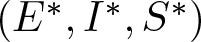 $(E^*,I^*,S^*)$ if and only if
  $\mathcal R_0 \gt 1$, where
 \begin{equation}
\begin{cases}
I^*:=\displaystyle\frac{(a-b)\left[\beta\sigma K- (\alpha+a)(\sigma+a)\right]}{\beta[\beta\sigma K-a(a-b)]}, \\
E^*:=\displaystyle\frac{1}{\sigma}[(\alpha+a)I^*-\beta I^{*2}]=\displaystyle\frac{1}{\sigma}[(\alpha+a)-\beta I^{*}]I^*, \\[2mm]
S^*:=\displaystyle\frac{1}{\beta\sigma}[(\sigma+a)-\beta I^*][(\alpha+a)-\beta I^*].
\end{cases}
\end{equation}
\begin{equation}
\begin{cases}
I^*:=\displaystyle\frac{(a-b)\left[\beta\sigma K- (\alpha+a)(\sigma+a)\right]}{\beta[\beta\sigma K-a(a-b)]}, \\
E^*:=\displaystyle\frac{1}{\sigma}[(\alpha+a)I^*-\beta I^{*2}]=\displaystyle\frac{1}{\sigma}[(\alpha+a)-\beta I^{*}]I^*, \\[2mm]
S^*:=\displaystyle\frac{1}{\beta\sigma}[(\sigma+a)-\beta I^*][(\alpha+a)-\beta I^*].
\end{cases}
\end{equation} The constant  $ \mathcal{R}_0 $ is commonly referred to as the basic reproduction number for (1) (see [Reference Wang and Zhao35], for example). It serves as a threshold parameter that distinguishes between two distinct long-term outcomes of the disease: extinction when
  $ \mathcal{R}_0 \lt 1 $, and persistence or spreading when
  $ \mathcal{R}_0 \gt 1 $.
In this subsection, we investigate the spreading behaviour of (3) under the condition  $ \mathcal{R}_0 \gt 1 $. Our first task is to prove the following result.
Proposition 3.1. Suppose that  $\mathcal{R}_0 \gt 1$. If
  $h_\infty-g_\infty=\infty$, then
  $h_\infty=\infty$ and
  $g_\infty=-\infty$.
We will need the following eigenvalue problem:
 \begin{equation}
\left\{\begin{array}{ll}
(\sigma+a)\phi_1-\beta K \phi_2=\lambda \phi_1,\ \ &-l \lt x \lt l,\\
-D \phi_2^{''} -\sigma \phi_1+(\alpha+a)\phi_2=\lambda \phi_2,\ &-l \lt x \lt l,\\
\phi_1(\pm l)=\phi_2(\pm l)=0
\end{array}\right.
\end{equation}
\begin{equation}
\left\{\begin{array}{ll}
(\sigma+a)\phi_1-\beta K \phi_2=\lambda \phi_1,\ \ &-l \lt x \lt l,\\
-D \phi_2^{''} -\sigma \phi_1+(\alpha+a)\phi_2=\lambda \phi_2,\ &-l \lt x \lt l,\\
\phi_1(\pm l)=\phi_2(\pm l)=0
\end{array}\right.
\end{equation} Let  $(\eta_1,\Phi^*)$ be the principal eigenvalue and eigenfunction of (7), and
 \begin{eqnarray*}
\tilde{R}(l):=\displaystyle\frac{\sigma\beta K}{(\eta_1(l)+\alpha+a)(\sigma+a)}=\displaystyle\frac{\sigma\beta K}{\left(D\left(\displaystyle\frac{\pi}{2l}\right)^2+\alpha+a\right)\left(\sigma+a\right)}.
\end{eqnarray*}
\begin{eqnarray*}
\tilde{R}(l):=\displaystyle\frac{\sigma\beta K}{(\eta_1(l)+\alpha+a)(\sigma+a)}=\displaystyle\frac{\sigma\beta K}{\left(D\left(\displaystyle\frac{\pi}{2l}\right)^2+\alpha+a\right)\left(\sigma+a\right)}.
\end{eqnarray*} Applying the results for (6) but with  $b$ replaced by
  $a$, we have the following lemma.
Lemma 3.4. Problem (12) admits a unique principal eigenvalue
 \begin{equation*}
\tilde{\lambda}_1=\tilde{\lambda}_1(l):=\frac{\sigma+a+\alpha+a+\eta_1-\sqrt{[\sigma+a-(\alpha+a+\eta_1)]^2+4\sigma\beta K}}{2},
\end{equation*}
\begin{equation*}
\tilde{\lambda}_1=\tilde{\lambda}_1(l):=\frac{\sigma+a+\alpha+a+\eta_1-\sqrt{[\sigma+a-(\alpha+a+\eta_1)]^2+4\sigma\beta K}}{2},
\end{equation*}with associated eigenfunction  $(\tilde{\phi},\tilde{\psi})=(\displaystyle\frac{\beta K}{\sigma+a-\lambda}\Phi^*,\Phi^*)$, and
  $\tilde{\lambda}_1=0$ if and only if
  $\tilde{R}(l)=1$. Moreover,
  $(\tilde{R}(l)-1)\tilde{\lambda}_1 \lt 0$ for
  $\tilde{R}(l)\neq 1$,
  $\tilde{R}(l)$ is strictly increasing in
  $l$ and
 \begin{eqnarray*}
\lim_{l\rightarrow +\infty}\tilde{R}(l)=\displaystyle\frac{\beta \sigma K}{(\alpha+a)(\sigma+a)}=\mathcal{R}_0.
\end{eqnarray*}
\begin{eqnarray*}
\lim_{l\rightarrow +\infty}\tilde{R}(l)=\displaystyle\frac{\beta \sigma K}{(\alpha+a)(\sigma+a)}=\mathcal{R}_0.
\end{eqnarray*} Therefore, when  $\mathcal{R}_0 \gt 1$, there exists a unique
  $\tilde l_* \gt 0$ such that
  $\tilde{R}(\tilde l_*)=1$, and
 \begin{equation}
\tilde l_*:=\displaystyle\frac{\pi}{2}\sqrt{\frac{D(\sigma+a)}{\sigma \beta K-(\alpha+a)(\sigma+a)}} \gt l_*,
\end{equation}
\begin{equation}
\tilde l_*:=\displaystyle\frac{\pi}{2}\sqrt{\frac{D(\sigma+a)}{\sigma \beta K-(\alpha+a)(\sigma+a)}} \gt l_*,
\end{equation}where  $l_*$ is given by (8).
Lemma 3.5. Suppose that  $\mathcal{R}_0 \gt 1$ and
  $\tilde l_*$ is given by (13). If
  $h_\infty-g_{\infty}=\infty$, then for any
  $l \gt \tilde l_*$ and
  $r\in\mathbb{R}$ such that
  $[-l+r, l+r]\subset (g_\infty, h_\infty)$, there holds
 \begin{equation}
\limsup_{t\to\infty}\|(E(t,\cdot),I(t,\cdot),S(t,\cdot))-(0,0,K)\|_{L^\infty([-l+r, l+r])} \gt 0.
\end{equation}
\begin{equation}
\limsup_{t\to\infty}\|(E(t,\cdot),I(t,\cdot),S(t,\cdot))-(0,0,K)\|_{L^\infty([-l+r, l+r])} \gt 0.
\end{equation}Proof. Assume to the contrary that (14) does not hold, then there exist  $l_0 \gt l^*$,
  $r_0\in\mathbb{R}$ such that for every small
  $\epsilon_0 \gt 0$, there exists
  $t_0 \gt 0$ (depending on
  $\epsilon_0$) such that
 \begin{equation}
\begin{cases}
[-l_0+r_0, l_0+r_0]\subset (g(t),h(t))\,\text{for }t\geq t_0,
\\
E(t,x), I(t,x)\in (0, \epsilon_0), \ S(t,x)-K\in (-\epsilon_0, \epsilon_0) \\
\text{for } t\geq t_0,\ x\in[-l_0+r_0, l_0+r_0].
\end{cases}
\end{equation}
\begin{equation}
\begin{cases}
[-l_0+r_0, l_0+r_0]\subset (g(t),h(t))\,\text{for }t\geq t_0,
\\
E(t,x), I(t,x)\in (0, \epsilon_0), \ S(t,x)-K\in (-\epsilon_0, \epsilon_0) \\
\text{for } t\geq t_0,\ x\in[-l_0+r_0, l_0+r_0].
\end{cases}
\end{equation}It follows that
 \begin{equation}
\left\{\begin{array}{ll}
{E}_{t}\geq \beta( K-\epsilon_0) I-\sigma {E}\\
- \left[b+(a-b)\displaystyle\frac{K+3\epsilon_0}{K}\right]{E},\ \ &t \gt t_0, \ -l_0+r_0 \lt x \lt l_0+r_0,\\
{I}_{t}\geq D {I}_{xx}+\sigma {E}-\alpha {I}\\
- \left[b+(a-b)\displaystyle\frac{K+3\epsilon_0}{K}\right]{I} ,\ \ &t \gt t_0, \ -l_0+r_0 \lt x \lt l_0+r_0\\
{E}(t,x) \gt 0, \ {I}(t,x) \gt 0,\ \ &t \gt t_0, \ x=\pm l_0+r_0.
\end{array}\right.
\end{equation}
\begin{equation}
\left\{\begin{array}{ll}
{E}_{t}\geq \beta( K-\epsilon_0) I-\sigma {E}\\
- \left[b+(a-b)\displaystyle\frac{K+3\epsilon_0}{K}\right]{E},\ \ &t \gt t_0, \ -l_0+r_0 \lt x \lt l_0+r_0,\\
{I}_{t}\geq D {I}_{xx}+\sigma {E}-\alpha {I}\\
- \left[b+(a-b)\displaystyle\frac{K+3\epsilon_0}{K}\right]{I} ,\ \ &t \gt t_0, \ -l_0+r_0 \lt x \lt l_0+r_0\\
{E}(t,x) \gt 0, \ {I}(t,x) \gt 0,\ \ &t \gt t_0, \ x=\pm l_0+r_0.
\end{array}\right.
\end{equation} For any given small  $\epsilon\in(0,K)$, we consider the following auxiliary eigenvalue problem:
 \begin{equation}
\left\{\begin{array}{ll}
-\beta (K-\epsilon)\psi_\epsilon+\sigma\phi_\epsilon+\left[b+(a-b)\displaystyle\frac{K+3\epsilon}{K}\right]\phi_\epsilon=\lambda \phi_\epsilon,\ \ &-l_0 \lt x \lt l_0,\\[12pt]
-D \psi_\epsilon^{''} -\sigma \phi_\epsilon+\alpha\psi_\epsilon+\left[b+(a-b)\displaystyle\frac{K+3\epsilon}{K}\right]\psi_\epsilon=\lambda \psi_\epsilon,\ &-l_0 \lt x \lt l_0,\\
\phi_\epsilon(\pm l_0)=\psi_\epsilon(\pm l_0)=0.
\end{array}\right.
\end{equation}
\begin{equation}
\left\{\begin{array}{ll}
-\beta (K-\epsilon)\psi_\epsilon+\sigma\phi_\epsilon+\left[b+(a-b)\displaystyle\frac{K+3\epsilon}{K}\right]\phi_\epsilon=\lambda \phi_\epsilon,\ \ &-l_0 \lt x \lt l_0,\\[12pt]
-D \psi_\epsilon^{''} -\sigma \phi_\epsilon+\alpha\psi_\epsilon+\left[b+(a-b)\displaystyle\frac{K+3\epsilon}{K}\right]\psi_\epsilon=\lambda \psi_\epsilon,\ &-l_0 \lt x \lt l_0,\\
\phi_\epsilon(\pm l_0)=\psi_\epsilon(\pm l_0)=0.
\end{array}\right.
\end{equation} By using arguments similar to Lemma 3.4, we know that problem (17) admits a unique principal eigenvalue  $\lambda_\epsilon$ associated with a positive eigenfunction
  $(\phi_\epsilon,\psi_\epsilon)$. Thanks to
  $\mathcal{R}_0 \gt 1$, it follows from Lemma 3.4 that
  $\tilde{\lambda}_1(l) \lt 0$ for any fixed
  $l \gt \tilde l_*$. Now that
  $\lim_{\epsilon\to 0}\lambda_\epsilon=\tilde{\lambda}_1(l_0) \lt 0$, we can find
  $\epsilon_0\in(0,K)$ small enough such that
  $\lambda_{\epsilon_0} \lt 0$.
Since  ${E}(t_0,x) \gt 0$ and
  ${I}(t_0,x)) \gt 0$ for
  $x\in[-l_0+r_0,l_0+r_0]$, we can find a small number
  $\theta \gt 0$ such that
 \begin{equation*}
{E}(t_0,x)\geq \theta\phi^{\epsilon_0}(x-r_0), {I}(t_0,x-r_0)\geq \theta\psi^{\epsilon_0}(x) \text{for } x\in[-l_0+r_0,l_0+r_0].
\end{equation*}
\begin{equation*}
{E}(t_0,x)\geq \theta\phi^{\epsilon_0}(x-r_0), {I}(t_0,x-r_0)\geq \theta\psi^{\epsilon_0}(x) \text{for } x\in[-l_0+r_0,l_0+r_0].
\end{equation*}Set
 \begin{equation*}
\underline{E}:=\theta e^{-\lambda_{\epsilon_0}(t-t_0)}\phi_{\epsilon_0}(x-r_0), ~~\underline{I}:=\theta e^{-\lambda_{\epsilon_0}(t-t_0)}\psi_{\epsilon_0}(x-r_0).
\end{equation*}
\begin{equation*}
\underline{E}:=\theta e^{-\lambda_{\epsilon_0}(t-t_0)}\phi_{\epsilon_0}(x-r_0), ~~\underline{I}:=\theta e^{-\lambda_{\epsilon_0}(t-t_0)}\psi_{\epsilon_0}(x-r_0).
\end{equation*} Using (17) with  $\epsilon=\epsilon_0$, we can easily verify that
  $(\underline{E},\underline{I})$ is a lower solution of (16). By applying the usual comparison principle, we obtain
 \begin{align*}
&\tilde{E}(t,x)\geq \theta e^{|\lambda_{\epsilon_0}|(t-t_0)}\phi_{\epsilon_0}(x), \tilde{I}(t,x)\\
&\quad \geq \theta e^{|\lambda_{\epsilon_0}|(t-t_0)}\psi_{\epsilon_0}(x) ~~\text{for }t\geq t_0, x\in(-l_0+r_0,l_0+r_0),
\end{align*}
\begin{align*}
&\tilde{E}(t,x)\geq \theta e^{|\lambda_{\epsilon_0}|(t-t_0)}\phi_{\epsilon_0}(x), \tilde{I}(t,x)\\
&\quad \geq \theta e^{|\lambda_{\epsilon_0}|(t-t_0)}\psi_{\epsilon_0}(x) ~~\text{for }t\geq t_0, x\in(-l_0+r_0,l_0+r_0),
\end{align*}Lemma 3.6. Suppose that  $\mathcal{R}_0 \gt 1$. If
  $h_\infty-g_{\infty}=\infty$, then for any
  $l \gt \tilde l_*$ and
  $r\in\mathbb{R}$ such that
  $[-l+r, l+r]\subset (g_\infty, h_\infty)$, we have
 \begin{equation}
\limsup_{t\to\infty}\|I(t,\cdot)\|_{L^\infty([-l+r, l+r])} \gt 0.
\end{equation}
\begin{equation}
\limsup_{t\to\infty}\|I(t,\cdot)\|_{L^\infty([-l+r, l+r])} \gt 0.
\end{equation}Proof. Assume to the contrary that there exist some  $l_1 \gt \tilde l_*$,
  $r_1\in \mathbb{R}$ such that
  $[-l_1+r_1, l_1+r_1]\subset (g^\infty,h^\infty)$ and
  $ \limsup_{t\to\infty}\|I(t,\cdot)\|_{L^\infty([-l_1+r_1, l_1+r_1])}=0$. It follows that
 \begin{equation}\lim_{t\to\infty} \|I(t,\cdot)\|_{L^\infty([-l_1+r_1,l_1+r_1])}= 0.
\end{equation}
\begin{equation}\lim_{t\to\infty} \|I(t,\cdot)\|_{L^\infty([-l_1+r_1,l_1+r_1])}= 0.
\end{equation} Let  $\epsilon_k$ be a positive sequence converging to 0 as
  $k\to\infty$. Then there exists
  $t_k\to\infty$ such that
 \begin{equation*}
0 \lt \beta L_1 I(t,x)\leq \epsilon_k \mbox{for } t\geq t_k, \ x\in [-l_1+r_1, l_1+r_1]\subset (g(t_k), h(t_k)).
\end{equation*}
\begin{equation*}
0 \lt \beta L_1 I(t,x)\leq \epsilon_k \mbox{for } t\geq t_k, \ x\in [-l_1+r_1, l_1+r_1]\subset (g(t_k), h(t_k)).
\end{equation*}It follows that
 \begin{align*}
&E_{t}=\beta I S-\sigma E- \left[b+(a-b)\displaystyle\frac{E+I+S}{K}\right] E\\
&\quad\leq \epsilon_k-(\sigma+b)E \ \mbox{for } t\geq t_k, \ x\in [-l_1+r_1, l_1+r+1].
\end{align*}
\begin{align*}
&E_{t}=\beta I S-\sigma E- \left[b+(a-b)\displaystyle\frac{E+I+S}{K}\right] E\\
&\quad\leq \epsilon_k-(\sigma+b)E \ \mbox{for } t\geq t_k, \ x\in [-l_1+r_1, l_1+r+1].
\end{align*} Therefore, for  $t \gt 0$ and
  $x\in [-l_1+r_1, l_1+r_1]$,
 \begin{equation*}
E(t,x)\leq E(0,x)e^{-(\sigma+b)(t)}+\epsilon_k\frac{1-e^{-(\sigma+b)(t)}}{\sigma+b}\leq L_1 e^{-(\sigma+b)t}+\frac{\epsilon_k}{\sigma+b}.
\end{equation*}
\begin{equation*}
E(t,x)\leq E(0,x)e^{-(\sigma+b)(t)}+\epsilon_k\frac{1-e^{-(\sigma+b)(t)}}{\sigma+b}\leq L_1 e^{-(\sigma+b)t}+\frac{\epsilon_k}{\sigma+b}.
\end{equation*}Hence
 \begin{equation*}
\limsup_{t\to\infty} E(t,x)\leq \frac{\epsilon_k}{\sigma+b}\,\mbox{uniformly for } x\in [-l_1+r_1,l_1+r_1].
\end{equation*}
\begin{equation*}
\limsup_{t\to\infty} E(t,x)\leq \frac{\epsilon_k}{\sigma+b}\,\mbox{uniformly for } x\in [-l_1+r_1,l_1+r_1].
\end{equation*} Letting  $k\to\infty$ we deduce
 \begin{equation}
\lim_{t\to\infty} E(t,x)=0\,\mbox{uniformly for } \ x\in [-l_1+r_1,l_1+r_1].
\end{equation}
\begin{equation}
\lim_{t\to\infty} E(t,x)=0\,\mbox{uniformly for } \ x\in [-l_1+r_1,l_1+r_1].
\end{equation}Clearly
 \begin{equation*}
S_{t}=(a-b)S\left(1-\displaystyle\frac{E+I+S}{K}\right)-\beta I S\leq (a-b)S\left(1-\displaystyle\frac{S}{K}\right) \mbox{for } \ t \gt 0, \ x\in\mathbb{R}.
\end{equation*}
\begin{equation*}
S_{t}=(a-b)S\left(1-\displaystyle\frac{E+I+S}{K}\right)-\beta I S\leq (a-b)S\left(1-\displaystyle\frac{S}{K}\right) \mbox{for } \ t \gt 0, \ x\in\mathbb{R}.
\end{equation*}It follows easily that
 \begin{equation}
\limsup_{t\to\infty} S(t,x)\leq K\,\mbox{uniformly for } x\in\mathbb{R}.
\end{equation}
\begin{equation}
\limsup_{t\to\infty} S(t,x)\leq K\,\mbox{uniformly for } x\in\mathbb{R}.
\end{equation} On the other hand, by (19) and (20), there exists  $s_k\to\infty$ such that
 \begin{equation*}
0\leq \frac{E(t,x)+I(t,x)}K+\frac\beta{a-b}I(t,x) \leq k^{-1}\,\mbox{for } t\geq s_k,\ x\in [-l_1+r_1, l_1+r_1].
\end{equation*}
\begin{equation*}
0\leq \frac{E(t,x)+I(t,x)}K+\frac\beta{a-b}I(t,x) \leq k^{-1}\,\mbox{for } t\geq s_k,\ x\in [-l_1+r_1, l_1+r_1].
\end{equation*}It follows that
 \begin{equation*}
S_{t}\geq (a-b)S\left(1-k^{-1}-\displaystyle\frac{S}{K}\right) \mbox{for } \ t\geq s_k, \ x\in
[-l_1+r_1, l_1+r_1].
\end{equation*}
\begin{equation*}
S_{t}\geq (a-b)S\left(1-k^{-1}-\displaystyle\frac{S}{K}\right) \mbox{for } \ t\geq s_k, \ x\in
[-l_1+r_1, l_1+r_1].
\end{equation*} Since  $m_k:=\min_{x\in[-l_1+r_1, l_1+r_1]}S(s_k, x) \gt 0$, the above differential inequality for
  $S$ implies
 \begin{equation*}
\liminf_{t\to\infty}S(t,x)\geq (1-k^{-1})K\,\mbox{uniformly for } x\in [-l_1+r_1, l_1+r_1].
\end{equation*}
\begin{equation*}
\liminf_{t\to\infty}S(t,x)\geq (1-k^{-1})K\,\mbox{uniformly for } x\in [-l_1+r_1, l_1+r_1].
\end{equation*} Letting  $k\to\infty$ we obtain
 \begin{equation*}
\liminf_{t\to\infty}S(t,x)\geq K\,\mbox{uniformly for } x\in [-l_1+r_1, l_1+r_1].
\end{equation*}
\begin{equation*}
\liminf_{t\to\infty}S(t,x)\geq K\,\mbox{uniformly for } x\in [-l_1+r_1, l_1+r_1].
\end{equation*} This and (21) imply  $S(t,x)\to K$ as
  $t\to\infty$ uniformly for
  $x\in [-l_1+r_1, l_1+r_1]$. Together with (19) and (20), this leads to a contradiction to Lemma 3.5. The lemma is now proved.
Proof of Proposition 3.1
Without loss of generality, we assume to the contrary that  $h_\infty \lt \infty$ and
  $g^\infty=-\infty$. Define
 \begin{equation*}
y:=\frac{x}{h(t)},\ z_1(t,y):=E(t,x), \ z_2(t,y):=I(t,x),\ z_3(t,y):=S(t,x).
\end{equation*}
\begin{equation*}
y:=\frac{x}{h(t)},\ z_1(t,y):=E(t,x), \ z_2(t,y):=I(t,x),\ z_3(t,y):=S(t,x).
\end{equation*} Then  $z_2$ solves
 \begin{equation*}
\begin{cases}
z_{2t}-\frac{D}{h^2(t)} z_{2yy}-\frac{h'(t)y}{h(t)}z_{2y}=f_2(z_1,z_2,z_3),&t \gt 0,\ y\in(\frac{g(t)}{h(t)},1),\\
z_2(t,\frac{g(t)}{h(t)})=z_2(t,1)=0,& t \gt 0,\\
h'(t)=-\frac{\mu}{h(t)}z_{2y}(t,1),&t \gt 0,\\
z_2(0,y)=I_0\left(h(t)y\right), &y\in[-1,1].
\end{cases}
\end{equation*}
\begin{equation*}
\begin{cases}
z_{2t}-\frac{D}{h^2(t)} z_{2yy}-\frac{h'(t)y}{h(t)}z_{2y}=f_2(z_1,z_2,z_3),&t \gt 0,\ y\in(\frac{g(t)}{h(t)},1),\\
z_2(t,\frac{g(t)}{h(t)})=z_2(t,1)=0,& t \gt 0,\\
h'(t)=-\frac{\mu}{h(t)}z_{2y}(t,1),&t \gt 0,\\
z_2(0,y)=I_0\left(h(t)y\right), &y\in[-1,1].
\end{cases}
\end{equation*} Using similar arguments as those in the proof of Lemma 3.3, we have  $h'(t)\to 0$ as
  $t\to\infty$.
Fix  $l \gt \tilde l_*$ and
  $r\in\mathbb{R}$ such that
  $[-l+r, l+r]\subset (g_\infty, h_\infty)$. By Lemma 3.6, there is a positive sequence
  $\{t_n\}$ such that
  $t_n\to\infty$ as
  $n\to\infty$ and
 \begin{equation}
\limsup_{t\to\infty}\|I(t,\cdot)\|_{L^\infty([-l+r, l+r])}= \lim_{m\to\infty}\|I(t_n,\cdot)\|_{L^\infty([-l+r, l+r])} \gt 0.
\end{equation}
\begin{equation}
\limsup_{t\to\infty}\|I(t,\cdot)\|_{L^\infty([-l+r, l+r])}= \lim_{m\to\infty}\|I(t_n,\cdot)\|_{L^\infty([-l+r, l+r])} \gt 0.
\end{equation}Define
 \begin{equation*}
Z_{1n}(t,y):=z_1(t+t_n,y),\ Z_{2n}(t,y):=z_2(t+t_n,y),\ Z_{3n}(t,y):=z_3(t+t_n,y).
\end{equation*}
\begin{equation*}
Z_{1n}(t,y):=z_1(t+t_n,y),\ Z_{2n}(t,y):=z_2(t+t_n,y),\ Z_{3n}(t,y):=z_3(t+t_n,y).
\end{equation*} Since  $Z_{1n}$ and
  $Z_{3n}$ are uniformly bounded, there exists
  $W_i, i=1,3,$ such that, upon extraction of a subsequence,
  $Z_{in}\to W_i$ weakly in
  $L_{loc}^p(\mathbb{R}\times(-\infty,1])$ for
  $p \gt 1$ and
  $i=1,3$. Furthermore, by applying the
  $L^p$ estimates to the equation satisfied by
  $Z_{2n}$ and using the Sobolev embedding theorem, we see that, upon extracting a subsequence,
  $Z_{2n}\to W_2$ in
  $C_{loc}^{(1+\gamma)/2,1+\gamma}(\mathbb{R}\times(-\infty,1])$ with the function
  $W_2$ satisfying the following problem in the weak sense:
 \begin{equation}
\begin{cases}
W_{2t}-\frac{D}{h_\infty^2} W_{2yy}=f_2(W_1,W_2,W_3),&t\in\mathbb{R},\ y\in(-\infty,1),\\
W_{2y}(t,1)=0,&t\in\mathbb{R},\\
W_2(t,1)=0, &t\in\mathbb{R}.
\end{cases}
\end{equation}
\begin{equation}
\begin{cases}
W_{2t}-\frac{D}{h_\infty^2} W_{2yy}=f_2(W_1,W_2,W_3),&t\in\mathbb{R},\ y\in(-\infty,1),\\
W_{2y}(t,1)=0,&t\in\mathbb{R},\\
W_2(t,1)=0, &t\in\mathbb{R}.
\end{cases}
\end{equation} By the standard  $L^p$ theory, we see that
  $W_2$ is a strong solution of (23). Since
  $W_1, W_2, W_3\geq 0$, we can apply the strong maximum principle to (23) to conclude that either
  $W_2\equiv 0$ or
  $W_2(t,y) \gt 0$ for
  $t\in\mathbb{R}$ and
  $y \lt 1$, and in the latter case, the Hopf boundary lemma implies
  $W_{2y}(t,1) \lt 0$, which contradicts the second equation in (23). Therefore, we necessarily have
  $W_2\equiv 0$. But this is a contradiction to (22). Hence
  $h_\infty=\infty$. The proof is complete.
The following result describes the spreading case, where the infected region spreads to the entire available space and the rabid fox population persists weakly.
Theorem 3.4. Suppose that  $\mathcal{R}_0 \gt 1$. If
  $h_\infty-g_{\infty}=\infty$, then
  $(g_\infty, h_\infty)=(-\infty, \infty)$, and for any
  $l \gt 0$, we have
 \begin{equation}
\limsup_{t\to\infty}\min_{x\in [-l, l]}I(t,x) \gt 0.
\end{equation}
\begin{equation}
\limsup_{t\to\infty}\min_{x\in [-l, l]}I(t,x) \gt 0.
\end{equation}Proof. By Lemma 3.6 and Proposition 3.1, we know that  $-g_\infty=h_\infty=\infty$ and
 \begin{equation*}
\limsup_{t\to\infty}\max_{x\in [-l, l]}I(t,x) \gt 0\,\mbox{for every } l \gt \tilde l_*.
\end{equation*}
\begin{equation*}
\limsup_{t\to\infty}\max_{x\in [-l, l]}I(t,x) \gt 0\,\mbox{for every } l \gt \tilde l_*.
\end{equation*} We now fix an arbitrary  $l \gt \tilde l_*$ and let
  $t_n\to\infty$ be a sequence satisfying
 \begin{equation}
0 \lt \limsup_{t\to\infty}\max_{x\in [-l, l]}I(t,x)=\lim_{n\to\infty}\max_{x\in [-l, l]}I(t_n,x).
\end{equation}
\begin{equation}
0 \lt \limsup_{t\to\infty}\max_{x\in [-l, l]}I(t,x)=\lim_{n\to\infty}\max_{x\in [-l, l]}I(t_n,x).
\end{equation}Clearly (24) will follow if we can show
 \begin{equation*}
\limsup_{n\to\infty}\min_{x\in [-l, l]}I(t_n,x) \gt 0.
\end{equation*}
\begin{equation*}
\limsup_{n\to\infty}\min_{x\in [-l, l]}I(t_n,x) \gt 0.
\end{equation*} Arguing indirectly we assume that  $\limsup_{n\to\infty}\min_{x\in [-l, l]}I(t_n,x)=0$, which implies
 \begin{equation*}\lim_{n\to\infty}\min_{x\in [-l, l]}I(t_n,x)=0.
\end{equation*}
\begin{equation*}\lim_{n\to\infty}\min_{x\in [-l, l]}I(t_n,x)=0.
\end{equation*} Let  $x_n\in [-l,l]$ satisfy
  $\min_{x\in [-l,l]}I(t_n, x)=I(t_n, x_n)$ and define
 \begin{equation*}
E_{n}(t,x):=E(t+t_n,x+x_n),\ I_{n}(t,x):=I(t+t_n,x+x_n),\ S_{n}(t,x):=S(t+t_n,x+x_n).
\end{equation*}
\begin{equation*}
E_{n}(t,x):=E(t+t_n,x+x_n),\ I_{n}(t,x):=I(t+t_n,x+x_n),\ S_{n}(t,x):=S(t+t_n,x+x_n).
\end{equation*} Since  $E_n$ and
  $S_n$ are uniformly bounded, there exist
  $E^*$ and
  $S^*$ such that, for any
  $p \gt 1$, upon extraction of a subsequence,
  $E_n$ and
  $S_n$ converges weakly in
  $L_{loc}^p(\mathbb{R}\times\mathbb{R})$ to
  $E^*$ and
  $S^*$, respectively. Furthermore, by applying the
  $L^p$ estimates to the equation satisfied by
  $I_n$ and using the Sobolev embedding theorem, we see that, upon extracting a subsequence,
  $I_n\to I^*$ in
  $C_{loc}^{(1+\gamma)/2,1+\gamma}(\mathbb{R}\times\mathbb{R})$ with the function
  $I^*$ satisfying the following problem in the weak sense (and hence in the
  $W^{1,2}_p$ sense):
 \begin{equation}
I^*_t-DI^*_{xx}=f_2(E^*, I^*, S^*)\,\mbox{for } t\in\mathbb{R},\ x\in \mathbb{R}.
\end{equation}
\begin{equation}
I^*_t-DI^*_{xx}=f_2(E^*, I^*, S^*)\,\mbox{for } t\in\mathbb{R},\ x\in \mathbb{R}.
\end{equation} Moreover, since  $E_n$,
  $I_n$ and
  $S_n$ are nonnegative, and
  $I_n(0,0)\to 0$ and
  $n\to\infty$, we have
 \begin{equation*}
E^*\geq 0, \ S^*\geq 0,\ I^*\geq 0\,\mbox{and } I^*(0,0)=0.
\end{equation*}
\begin{equation*}
E^*\geq 0, \ S^*\geq 0,\ I^*\geq 0\,\mbox{and } I^*(0,0)=0.
\end{equation*}Since
 \begin{equation*}
f_2(E^*, I^*, S^*)=\sigma E^*-\left[\alpha I^*+b+(a-b)\displaystyle\frac{E+I^*+S^*}{K}\right]I^*,
\end{equation*}
\begin{equation*}
f_2(E^*, I^*, S^*)=\sigma E^*-\left[\alpha I^*+b+(a-b)\displaystyle\frac{E+I^*+S^*}{K}\right]I^*,
\end{equation*}and  $\alpha I^*+b+(a-b)\displaystyle\frac{E+I^*+S^*}{K}\in L^\infty(\mathbb{R}\times\mathbb{R})$, we can apply the strong maximum principle to (26) to deduce that
  $I^*\equiv 0$. It follows that
 \begin{equation*}
I(t_n, x)\to 0\,\mbox{uniformly for } x\in [-l,l] \mbox{as } n\to\infty.
\end{equation*}
\begin{equation*}
I(t_n, x)\to 0\,\mbox{uniformly for } x\in [-l,l] \mbox{as } n\to\infty.
\end{equation*}But this contradicts (25). Hence, the desired conclusion holds, and the proof is complete.
Next, we obtain some sufficient conditions for spreading.
Theorem 3.5. Suppose that  $\mathcal{R}_0 \gt 1$. Then spreading always happens if
  $h_0\geq \tilde l_*$, where
  $\tilde l_*$ is given by (13).
Proof. Since  $h_\infty-g_\infty \gt 2h_0$, it suffices to show that
  $h_\infty-g_\infty \lt \infty$ implies
  $h_{\infty}-g_\infty\leq\Lambda:=2\tilde l_*$. Suppose on the contrary that
  $h_{\infty}-g_\infty \gt \Lambda$, then we can find
  $T,l \gt 0$ such that
 \begin{equation*}
h(t)-g(t)\geq h(T)-g(T) \gt 2l \gt \Lambda\,\text{for }t\geq T.
\end{equation*}
\begin{equation*}
h(t)-g(t)\geq h(T)-g(T) \gt 2l \gt \Lambda\,\text{for }t\geq T.
\end{equation*} Hence, for any given  $r\in(g(T)+l,h(T)-l)$, there holds
 \begin{equation*}
[-l+r, l+r]\subset (g(T),h(T))\subset (g(t),h(t))\,\text{for }t\geq T.
\end{equation*}
\begin{equation*}
[-l+r, l+r]\subset (g(T),h(T))\subset (g(t),h(t))\,\text{for }t\geq T.
\end{equation*}Define
 \begin{equation*}\tilde{E}(t,x)=E(t,x+r),\tilde{I}(t,x)=I(t,x+r),\tilde{S}(t,x)=S(t,x+r)\text{for }t\geq T,x\in [-l,l].\end{equation*}
 By Lemma 3.1, we see that (15) and (16) hold for  $(l_0, r_0)=(l,r)$ and some
  $t_0\geq T$. Let
  $\underline{E}$ and
  $\underline{I}$ be the functions as constructed in the proof of Lemma 3.5. Then the arguments used there can be repeated to show that
  $(\underline{E},\underline{I})$ is a lower solution of (16) in the region
  $D=\{(t,x):t\geq t_0,-l\leq x\leq l\}$. Hence,
 \begin{equation*}
\tilde{E}(t,x)\geq \underline{E}(t,x), \tilde{I}(t,x)\geq \underline{I}(t,x)\,\text{for }(t,x)\in D,
\end{equation*}
\begin{equation*}
\tilde{E}(t,x)\geq \underline{E}(t,x), \tilde{I}(t,x)\geq \underline{I}(t,x)\,\text{for }(t,x)\in D,
\end{equation*}which leads to a contradiction in the same manner as in the proof of Lemma 3.5.
Theorem 3.6. Suppose that  $\mathcal{R}_0 \gt 1$ and
  $h_0 \lt \tilde l_*$ with
  $\tilde l_*$ given by (13). Then there exists
  $\mu_1$ depending on
  $E_0(x)$,
  $I_0(x)$ and
  $S_0(x)$ such that spreading happens if
  $\mu \gt \mu_1$.
Proof. By Lemma 2.1, we have
 \begin{eqnarray*}
\begin{cases}
I_{t}-DI_{xx}\geq -(\alpha+b) I, &t \gt 0, \ g(t) \lt x \lt h(t),\\
I(t,g(t))=I(t,h(t))=0, &t \gt 0\\
h'(t)=-\mu I_{x}(t,h(t)),\ &t \gt 0, \\
g'(t)=-\mu I_{x}(t,g(t)),\ &t \gt 0, \\
I(0,x)=I_{0}(x), \ & -h_0\leq x\leq h_0,\\
g(0)=-h_0,\ h(0)=h_0.
\end{cases}
\end{eqnarray*}
\begin{eqnarray*}
\begin{cases}
I_{t}-DI_{xx}\geq -(\alpha+b) I, &t \gt 0, \ g(t) \lt x \lt h(t),\\
I(t,g(t))=I(t,h(t))=0, &t \gt 0\\
h'(t)=-\mu I_{x}(t,h(t)),\ &t \gt 0, \\
g'(t)=-\mu I_{x}(t,g(t)),\ &t \gt 0, \\
I(0,x)=I_{0}(x), \ & -h_0\leq x\leq h_0,\\
g(0)=-h_0,\ h(0)=h_0.
\end{cases}
\end{eqnarray*}Denote
 \begin{equation*}
m_0:=\min_{x\in[-h_0/2,h_0/2]}I_0(x) \gt 0.
\end{equation*}
\begin{equation*}
m_0:=\min_{x\in[-h_0/2,h_0/2]}I_0(x) \gt 0.
\end{equation*} Let  $s(t):=\frac{h_0}{2}+t^2$ and
  $w_0\in C^{2+\gamma}$ be a function satisfying
 \begin{equation*}
w_0(\pm \frac{h_0}{2})=0, w'_0(-\frac{h_0}{2}) \gt 0 \gt w'_0(\frac{h_0}{2}),0 \lt w_0(x) \lt m_0\,\text{for }x\in(-\frac{h_0}{2},\frac{h_0}{2}).
\end{equation*}
\begin{equation*}
w_0(\pm \frac{h_0}{2})=0, w'_0(-\frac{h_0}{2}) \gt 0 \gt w'_0(\frac{h_0}{2}),0 \lt w_0(x) \lt m_0\,\text{for }x\in(-\frac{h_0}{2},\frac{h_0}{2}).
\end{equation*}Then consider the following initial boundary value problem:
 \begin{equation*}
\begin{cases}
w_t-Dw_{xx}=-(\alpha+b)w,&t \gt 0, \ -s(t) \lt x \lt s(t),\\
w(t,\pm s(t))=0,\ &t \gt 0, \\
w(0,x)=w_0(x) , &x\in[-h_0/2,h_0/2].
\end{cases}
\end{equation*}
\begin{equation*}
\begin{cases}
w_t-Dw_{xx}=-(\alpha+b)w,&t \gt 0, \ -s(t) \lt x \lt s(t),\\
w(t,\pm s(t))=0,\ &t \gt 0, \\
w(0,x)=w_0(x) , &x\in[-h_0/2,h_0/2].
\end{cases}
\end{equation*} By the standard parabolic Schauder theory, this problem admits a unique classical solution  $w(t,x)$. The maximum principle and Hopf boundary lemma imply that
 \begin{equation}
0 \lt w(t,x) \lt m_0,\ w_x(t,s(t)) \lt 0 \lt w_x(t,-s(t))\,\text{for }t\geq0,x\in(-s(t),s(t)).
\end{equation}
\begin{equation}
0 \lt w(t,x) \lt m_0,\ w_x(t,s(t)) \lt 0 \lt w_x(t,-s(t))\,\text{for }t\geq0,x\in(-s(t),s(t)).
\end{equation} Setting  $T:=\sqrt{2\tilde l_*-h_0}$, then we can find a large number
  $\mu_1 \gt 0$ such that
 \begin{equation*}
s'(t)=2t\leq \mp\mu w_x(t,\pm s(t))\,\text{for }t\in[0,T]\,\text{and }\mu\geq \mu_1.
\end{equation*}
\begin{equation*}
s'(t)=2t\leq \mp\mu w_x(t,\pm s(t))\,\text{for }t\in[0,T]\,\text{and }\mu\geq \mu_1.
\end{equation*}Moreover, it is clear that
 \begin{equation*}
I(t,x)\geq 0=w(t,x)\ \text{for}\ t \gt 0\ \text{and}\ x\in[g(t),h(t)]\cap\{- s(t),s(t)\}.
\end{equation*}
\begin{equation*}
I(t,x)\geq 0=w(t,x)\ \text{for}\ t \gt 0\ \text{and}\ x\in[g(t),h(t)]\cap\{- s(t),s(t)\}.
\end{equation*}Hence, we can apply the comparison principle (see Lemma 5.7 and Remark 5.8 of [Reference Du and Lin10]) to obtain that
 \begin{equation*}
[-s(t),s(t)]\subseteq [g(t),h(t)]\,\text{for }t\in[0,T]\,\text{and }\mu\geq \mu_1,
\end{equation*}
\begin{equation*}
[-s(t),s(t)]\subseteq [g(t),h(t)]\,\text{for }t\in[0,T]\,\text{and }\mu\geq \mu_1,
\end{equation*}which yields that
 \begin{equation*}
h_\infty-g_\infty \gt h(T)-g(T)\geq 2s(T)=\Lambda\,\text{for } \mu\geq \mu_1.
\end{equation*}
\begin{equation*}
h_\infty-g_\infty \gt h(T)-g(T)\geq 2s(T)=\Lambda\,\text{for } \mu\geq \mu_1.
\end{equation*}The desired result then follows easily from Theorem 3.5.
3.3. Further discussions
We end the paper with some discussions on the model and on possible directions of future work. A striking feature of the model (3) is the lack of diffusion in the equations for  $E$ and
  $S$, and the free boundaries in the
  $I$ equation. These are biologically meaningful since
  $E$ and
  $S$ are known to be territorial, and only
  $I$ moves to areas beyond its original territory due to the effect of the disease, and the range of
  $I$ is expanding because of that, which is the main cause for the spreading of the disease.
These assumptions lead to mathematical difficulties, in terms of the proof of the well-posedness of the model itself, as well as for the description of the long-time dynamics. While the former difficulty was overcome in this paper, and the case of vanishing is reasonably well-understood, the mathematical description for the case of spreading is a little weak, where we only managed to prove the weak persistence of  $I$ in Theorem 3.4. We propose the following conjecture:
Open Problem. We believe that strong persistence of  $I$ holds in the spreading case, namely in Theorem 3.4 the conclusion can be strengthened to
 \begin{equation*}
(g_\infty, h_\infty)=(-\infty,\infty)\,\mbox{and } \liminf_{t\to\infty}\min_{x\in [-l, l]}I(t,x) \gt 0\,\mbox{for any } l \gt 0.
\end{equation*}
\begin{equation*}
(g_\infty, h_\infty)=(-\infty,\infty)\,\mbox{and } \liminf_{t\to\infty}\min_{x\in [-l, l]}I(t,x) \gt 0\,\mbox{for any } l \gt 0.
\end{equation*} We think that the reason we have been unable to prove the strong persistence of  $I$ here is a technical one, caused by the lack of compactness of the functions
  $\{(E(t,\cdot), S(t,\cdot)): t \gt 0\}$ in a suitable function space, due to not enough regularity of the ODE solutions in the system can be obtained so far.
For future work, in the case of spreading, an important question left untouched here is about the spreading speed. It would be interesting to investigate the associated semi-wave problem of (3) and try to use it to determine the spreading speed of the disease.
As both a reasonable variation of (3) and also as a way to tackle the above open problem on the strong persistence of  $I$ in the spreading case, it might be worthwhile to add a diffusion term in the
  $E$ and
  $S$ equations of (3), say
  $\epsilon E_{xx}$ and
  $\epsilon S_{xx}$, respectively, with
  $0 \lt \epsilon\ll1$, and see how the solution of the perturbed system behaves and whether it converges to that of (3) as
  $\epsilon\to 0$.
Acknowledgements
The research of Y. Zhang was supported by NSFC grant 11626072, Chunhui Project Foundation of the Education Department of China 202201200 and CSC Grant 202308230246, and part of this work was completed while he was visiting the University of New England. Y. Du and Z. Ma were supported by the Australian Research Council.

 Open access