Learning and growth toward the frontier

During the first phase of their lives, individuals invest in parallel in the growth of their personal capital x and the learning of the available knowledge z (i.e. in the conversion of public capital z into personal capital y). In Supporting Information A.1.1, we show that this phase lasts for a time

$$\tau _1\lpar z \rpar = \displaystyle{z \over \lambda }\displaystyle{{\kappa + 1} \over \kappa }$$

Pure growth toward the frontier

Once z is fully socially learned, the capital y can potentially continue to increase if individuals invest in innovation. However, since the efficiency of innovation is lower than the efficiency of social learning, this implies that, at the end of Phase 1, investing in growth is necessarily more profitable than innovating. So individuals do not start innovating right away. They first experience a phase during which they only invest in the growth of x. They do so until the value of investing in x becomes as low as the value of innovating, at which point they start innovating. In Supporting Information A.1.2, we show that this second phase lasts for a time

$$\tau _2\lpar z \rpar = \displaystyle{{\lambda -\eta } \over {\lambda \eta \kappa }}z$$

Hence, catching up takes a total time τ(z) ≡ τ ₁(z) + τ ₂(z), which allows us to define the average growth rate of individuals during the catch-up phase

(2)$$r_c\equiv \displaystyle{z \over {\tau \lpar z \rpar }} = \displaystyle{{\lambda \eta \kappa } \over {\lambda + \eta \kappa }}$$

Innovation at the frontier and cultural interference

Once the frontier is reached, individuals start investing in innovation. However, they are not alone. Other individuals in the population also invest in innovation in parallel. Here we assume that individuals are aware of the innovations made, or in the process of being made, by others. As a result, since it is more efficient to learn something socially than to reinvent it by oneself, individuals always decide to focus on innovations that are not already made by others, which results in a sharing of the innovation work. This does not mean that we assume individuals to be cooperative, however. On the contrary, individuals always behave so as to maximize their own self-interest, but they do so by taking into account others’ behaviour. In Supporting Information A.1.3, we show that the rate at which a population of N individuals produces new knowledge under this assumption is

(3)$$r_i = \displaystyle{{\lambda \eta \kappa N} \over {\lambda \lpar {N + \kappa } \rpar + \eta \kappa \lpar {N-1} \rpar }}$$

This shows that population size, N, has a positive but saturating effect on the rate of cultural evolution at the frontier (the derivative of r _i with respect to N is positive but decreasing, and it tends towards 0 when N tends towards infinity). As a result, the rate of cultural evolution increases with N but asymptotically tends towards a maximum,

$$\displaystyle{{\lambda \eta \kappa } \over {\lambda + \eta \kappa }}$$

for large population sizes. This is a consequence of the fact that individuals must spend time learning the innovations made by others, which forces them to divert resources away from their own innovations. In other words, if more heads means more ideas, it also implies more ideas to learn, and therefore less time available to create new ideas. In parallel with the notion of selective interference, which limits the speed of biological adaptation, we call this phenomenon ‘cultural interference’.

The limits of cultural accumulation

If a population contains an amount of knowledge z in a generation, in the next generation it contains an amount

(4)$${z}^{\prime} = z + r_i\left({L-\displaystyle{z \over {r_c}}} \right) = r_iL + \displaystyle{{r_c-r_i} \over {r_c}}z$$

where r _c and r _i are given respectively by eqs (2) and (3) above, resulting in a linear recurrence equation that can be solved and plotted (see eq. 6 in Supporting Information, and Figure 2). This shows three things.

Figure 2.

Cultural dynamics in model 1. Here we plot the dynamics of heritable capital through generations for 20 different values of population size ranging from N = 1 (blue curve) to N = 2200 (red curve). Note that the curves are drawn as if cultural evolution was a continuous phenomenon even though, in reality, generations are discrete in our model. Parameters are as follows:γ = 1, λ = 5, η = 0.1, P ₀ = 0.1, L = 30, and κ = 0.1 (a), κ = 1 (b), κ = 10 (c) and κ = 100 (d).

First, the level of knowledge contained in a population converges towards an equilibrium, a cultural carrying capacity, independent of population size and given by

(5)$$z_{{\rm conv}} = \displaystyle{{\lambda \eta \kappa } \over {\lambda + \eta \kappa }}L$$

In addition to the total time budget available, L, this equilibrium depends on two limiting factors: the learning efficiency, λ, and the product ηκ, which depends both on the efficiency of investments into innovation, η, and on the relative importance of knowledge in the needs of individuals,κ. Even if the cost of social learning is not limiting (for example because λ is very large), the equilibrium amount of culture in a population is still limited by the fact that people waste time investing in non-heritable capital. Every investment in (a) learning existing knowledge and (b) growing non-heritable capital constitutes a loss for culture, as it must be re-made from scratch every generation. It must also be noted that this equilibrium depends on the efficiency of innovation, η, only provided κ is not infinite. In fact, η plays a role in the equilibrium level of culture by changing the relative attractiveness of investing in innovation as compared with investing in x. Therefore, if one ignores the existence of non-heritable capital (i.e. if κ is infinite), this effect disappears.

Second, cultural accumulation is always decelerating (see Figure 2) since the amount of newly produced culture from one generation to the next,

$${z}^{\prime}-z = r_iL-\displaystyle{{r_i} \over {r_c}}z$$

is a linearly decreasing function of z. This is a consequence of the fact that the technological frontier always recedes with the amount of existing knowledge, and this for two reasons. First, existing knowledge must be learnt before individuals start innovating, which takes time. Second, the more knowledge that already exists, the less further innovations are useful as compared with non-heritable capital and, therefore, the more individuals grow their x before they start innovating.

Third, this allows us to understand the conditions that make the existence of cumulative culture possible. Cultural accumulation occurs if the amount of cultural knowledge attained in a population in a given generation increases with the amount of cultural knowledge available in the previous generation. That is, if z ^′ is an increasing function of z. From eq. (4), we can see that this is the case provided that r _i < r _c. In other words, culture gradually accumulates provided the growth rate of individuals during catch-up is larger than their growth rate during the innovation phase. More precisely, eq. 4 shows that the parameter that governs the cultural accumulation potential in a population is the ratio

$$K\equiv \displaystyle{{r_c-r_i} \over {r_c}}$$

which is given by

(6)$$K\equiv \lpar {\lambda -\eta } \rpar \times \displaystyle{\kappa \over {\eta \kappa + \lambda }} \times \displaystyle{1 \over N}$$

This cumulative potential depends on three factors (see also Figure 2):

• • First, K increases with the difference between the efficiency of learning and the efficiency of innovation, λ − η. This is the most obvious factor. Culture accumulates on the condition that the cost of learning what has already been discovered is lower than the cost of discovering them initially.

• • Second, K increases with the proportion of knowledge in individuals’ capital, κ. The higher the knowledge content of individuals’ capital, the greater the cumulative potential. This second effect can also be understood for the same reason. When κ is low, the majority of the capital of individuals has to be reconstructed anyway at each generation from scratch, so there is no strong advantage given by the pre-existence of knowledge and culture is then hardly cumulative.

• • Lastly, K decreases with population size N. Culture accumulates provided population size is not too large. This counter-intuitive result can be understood by observing that, when N ≫ max(1, κ), the rate of cultural evolution during the innovation phase is approximately equal to the rate of evolution during the catch-up phase (r _i ≈ r _c; eqs 2 and 3). In a large population, even if innovation is less efficient than social learning (that is, even if λ > η), the vast majority of knowledge acquired by an individual is acquired through social learning, and not through innovation, anyway. Each individual needs to produce only a very small part of the knowledge by himself. It is therefore almost the same for an individual to grow up in a population in which there is already a quantity of information z produced by previous generations (and where the rate of cultural growth is therefore r _c), as to grow up in a large population that produces this information on the fly by innovation (and where the rate of cultural growth is therefore r _i ≈ r _c). Culture can therefore not accumulate in an infinite population. In contrast, in a small population, innovation is a limiting factor and therefore the rate of cultural evolution is significantly slower at the frontier than during catch-up, which leads to a gradual accumulation of knowledge.

Optimal growth schedule

As in model 1, we assume that individuals have a time L to develop (after which they reproduce) and we assume that they allocate their production optimally at all times to growth, learning and innovation, which implies that they always make the investment(s) that have the greatest marginal effect on production (see Supporting Information A.2). This optimal allocation consists of three phases, as in model 1. The only difference with model 1 is that, here, the growth of individuals is not linear. This growth cannot be expressed analytically, hence we simulate it numerically (see Supporting Information A.2). As in model 1, but numerically here, we derive the level of knowledge reached by a population of N individuals at generation t + 1 as a function of the level of knowledge at generation t.

Unlike in the first model, knowledge – or more generally heritable capital – can accumulate here from generation to generation even in a very large population (see Figures 3 and 4). This occurs because knowledge allows individuals to be more efficient in the production of new knowledge. As a result, knowledge first accumulates in an accelerating way. However, under this simple version of the model, the time it takes to reach the frontier nevertheless keeps on increasing as knowledge accumulates. At some point therefore, individuals do not have enough time left to innovate. As a result, the production of new knowledge eventually decelerates, until knowledge finally reaches an equilibrium.

Figure 3.

Cultural dynamics in model 2. Here we plot the dynamics of heritable capital through generations for 20 different values of population size ranging from N = 1 (blue curve) to N = 2200 (red curve). Parameters are as in Figure 2, with the time-step used in numerical simulations δ = 0.01

Figure 4.

Cultural evolution in model 2. (a) The thick solid line shows the amount of cultural capital in generation t + 1 plotted in function of cultural capital in generation t. The dashed line shows the identity function. This allows graphical representation of the dynamics of culture from any initial condition, by directly reading, at each generation, the amount of culture reached in the next generation (see the thin arrows). When culture is initially low, it increases. When culture is initially high, it decreases. In between, culture has a range of intermediate equilibria. (b) Graphic representation of cultural dynamics through an analogy with a physical landscape. This allows an intuitive perception of the dynamics by picturing the course of a ball going down the hills and stopping in the plain. The landscape is constructed by setting its slope for each value of z _t as being proportional to the change of cultural capital in one generation when starting from z _t. Parameters are as in Figure 3, with population size N = 1000.

This model also allows us to explore more subtle effects of culture on individuals’ life histories. In the following, we explore three biologically plausible effects and show that they often lead to more complex cultural dynamics.

Investments in knowledge increase along the pyramid of needs

It is reasonable to assume that the most basic needs of individuals are purely personal and not heritable. Individuals at the beginning of their growth invest mainly in their biological capital, that will be lost upon their death. It is only when they become richer, moving upward on their so-called pyramid of needs (Maslow, Reference Maslow1943), that they can begin to invest in forms of capital that are further away from biology, improving their environment at a larger scale, or investing in knowledge (see Baumard, Reference Baumard2018 for a review). Here, we capture this effect by assuming that the ratio κ is low when the amount of non-heritable capital, x, owned by an individual is below a threshold $\hat{x}$ and increases to a higher value when $x \gt \hat{x}$. Only wealthy enough individuals (in terms of personal capital) can afford to spend a large fraction of their resources on knowledge.

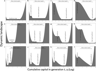
The consequences of this effect on cultural dynamics are shown in Figure 5(a–d). Culture accumulates and has phases of acceleration (not shown), because the existing knowledge allows individuals to be culturally more productive. What is more, for reasonable parameter values, culture can be bi-stable. On the one hand, a population starting initially without any cultural knowledge accumulates little culture and eventually remains stuck in a ‘poverty trap’ (Azariadis & Stachurski, Reference Azariadis and Stachurski2005), at a very low level of knowledge. On the other hand, if the amount of cultural knowledge exceeds a threshold, for stochastic reasons for example or because of a change in the environment, then individuals reach a state where they can afford to invest a larger fraction of their resources in knowledge. They then manage to capitalize from generation to generation, which allows them to reach eventually a much higher level of cultural knowledge.

Figure 5.

Cultural dynamics when culture is a capital. Graphic representation of cultural dynamics through an analogy with a physical landscape, as in Figure 4. (a–d) Investments in knowledge increase along the pyramid of needs, with parameters as in Figure 3, but with α = (1 − c)ζ and β = cζ, where ζ = 0.9, and c is a hard threshold function of x: c = c _low for $x \le \hat{x}$, and c = c _high for $x \gt \hat{x}$, with $\hat{x} = 3\cdot 10^5$, c _low = 0.05, and c _high = 0.05 (a), c _high = 0.1 (b), c _high = 0.5 (c) or c _high = 1 (d). (e–h) Age at maturity increases with cultural capital, with parameters as in Figure 3, but with the time available for growth, L, varying as a function of z according to a sigmoid function:$L\lpar z \rpar = L_{{\rm low}} + \lpar {L_{{\rm high}}-L_{{\rm low}}} \rpar z^2{\rm /}\lpar {{\hat{z}}^2 + z^2} \rpar$, with $\hat{z} = 10^4$, L _low = 10, and L _high = 10 (e), L _high = 30 (f), L _high = 50 (g), or L _high = 100 (h). (i–l) With division of labour, and parameters as in Figure 3, but with α = β = 0.5, and the division of labour model described in the section B of Supporting Information with λ _min = 0.01, ϕ = z, u = 1, and the exponent of the production cost varying in function of z according to eq. 18 in Supporting Information, with a _high = 2, a _low = 1, and σ = 10, and with population size N = 10 (i), N = 50 (j), N = 100 (k) or N = 1000 (l).

Parental care and age at first reproduction increase with the amount of cultural knowledge

The development of individuals depends, among other things, on two essential factors: the time during which they grow (that is, their age at maturity) and the amount of parental care they receive. Age at maturity is a life history decision of the offspring (Charnov, Reference Charnov1991; Stearns, Reference Stearns1977). Parental care is a life history decision of the parents, who can choose either to produce a large number of offspring with few resources for everyone, or a small number of offspring with a lot of resources for each.

Empirical observations show that these two aspects of life history are plastic in humans, and depend in particular on the level of resources of individuals (Nettle, Reference Nettle2010; Roser, Reference Roser2017). For instance, in the case of parental care, during their economic development, human societies make a relatively abrupt transition, the demographic transition, from a strategy with many children, each with relatively little investment, to a strategy with a high investment per child (Blanc & Wacziarg, Reference Blanc and Wacziarg2019; Cummins, Reference Cummins2013). A similar phenomenon occurs regarding the age at first reproduction. Economic development and increased levels of resources lead people, on average, to delay their reproduction and invest longer in their studies while, conversely, poverty leads women to choose to reproduce early (Roser, Reference Roser2017).

We have introduced these two types of plasticity into our model. Formally, the age at sexual maturity is captured by the parameter L, and parental care is captured by our parameter P ₀ measuring the productivity of individuals that is independent of their own capital. In both cases, for simplicity, we assume that they increase with the level of resources of the parental generation, that is L and/or P ₀ in generation t + 1 increase with the amount of knowledge z _t available in the previous generation. Here we show results in the case where only L is plastic. We assume that L( ⋅ ) is a sigmoid function, with a sudden change in strategy when z _t exceeds a threshold. This assumption leads, again, to bi-stable dynamics, with a sudden acceleration of cultural evolution when individuals’ life history strategy changes (Figure 5e–h). This occurs here because the knowledge of the previous generation directly accelerates the growth of the individuals of the next generation, and allows them to reach the frontier earlier in spite of the burden of knowledge.

We also included the possibility that the change of life history involved in the demographic transition may be accompanied by a reduction in population size. In reality, it has only been accompanied by a slowdown in population growth (not by a reduction of population size). However, the important point is that there is indeed a trade-off between population size and parental care (or duration of growth) per child. Since population size has a small effect on the dynamics of cultural accumulation, however, this effect did not counteract the positive effect of life history (not shown). Cultural accumulation is much more intense in a small population where each individual has a lot of parental care and a long period of growth than in a large population where each individual has little care and little time to grow.

Division of cognitive labour and the effective cost of learning

The efficiency of social learning itself can increase with the amount of cultural information available if, on average, the greater the amount of information produced in the past, the faster each unit of information is learned. This hypothesis is followed in many papers that assume the rate of social learning to be proportional to the amount of knowledge available that an individual does not yet not possess (e.g. Aoki et al., Reference Aoki, Wakano and Lehmann2012; Lehmann et al., Reference Lehmann, Wakano and Aoki2013). This assumption has no reason to be true in general. However, it is conceivable that sometimes it may be true, particularly if new cultural knowledge partially replaces old ones. Arabic numerals, for example, have replaced Roman numerals, and they are more useful but not more expensive to learn. The efficiency of social learning has therefore increased after the invention of Arabic numerals. More generally, people do not need to learn the whole history of science and technology, but simply to learn the latest state of the art. In addition, it is conceivable that part of cultural progress consists of improving existing knowledge by making it more compact, or easier to learn, and thus improving the efficiency of investments in social learning. Overall, therefore, the return on investment of social learning, λ, is likely to increase with z, which is a way for culture to increase the efficiency of individuals’ lives.

However, in fact, knowledge has a stronger and more general effect on the cost of learning through another mechanism. In practice, in any developed society with a large number of technologies, we acquire the benefits of the vast majority of cultural knowledge without having to learn it. For example, we benefit from our societies’ technical knowledge on internal combustion engines without having to learn anything, or almost anything, about the functioning, let alone the making, of these engines. Only a very small fraction of people in our societies invest in the acquisition of this knowledge. All of the others obtain the benefits of internal combustion engines by exchanging with these specialists.

Thus, the true cost of ‘learning’ a technique is not really the cost of learning it but rather the cost of acquiring the benefits of that technique via an exchange with others. This cost is lower because only one individual pays the cost of learning and then passes it on to all of their customers. Standard models of cultural evolution take into account the existence of a division of labour of innovation, which constitutes the major benefit of culture in these models. However, to capture the full benefits of culture, we must also take into account another division of labour: the division of labour of social learning.

This principle has an essential consequence. As technological progress creates economies of scale, it paradoxically reduces the effective cost of learning (that is, the cost of acquiring technical goods). The higher the level of technical knowledge in a society about food production, for example, the more a small number of producers can supply a large number of consumers at low prices. Thus, even if the cost of learning to become a farmer increases with the amount of technical knowledge (it requires longer and longer studies), the price of food can actually decrease, because this cost is passed on to a larger and larger number of consumers.

In Supporting Information section B, we formalize this principle with an approach inspired by micro-economic models of markets. The result of this analysis is illustrated in Figure 5(i–l). In a large population, we observe once again bi-stable dynamics, with a poverty trap at low technical level (and low division of labour) and a sudden acceleration beyond a threshold, towards a new equilibrium at high technical level (and high division of labour). This occurs here because the knowledge of the previous generation reduces the effective cost of ‘social learning’ for the next generation, which allows them to reach the frontier earlier in spite of the burden of knowledge. In addition, we also observe an indirect effect of population size as it constitutes an upper limit on the division of labour.