


Introduction
The Greenland ice sheet is losing mass at an accelerating rate, and since around the year 2000 the surface mass balance has become the dominant driver of ice sheet mass loss (van den Broeke and others, Reference van den Broeke2016; Bamber and others, Reference Bamber, Westaway, Marzeion and Wouters2018; the IMBIE Team, 2019). Increasing summer meltwater generation and associated runoff is the main driver of the declining surface mass balance, in particular in the southwestern part of the Greenland ice sheet (Nienow and others, Reference Nienow, Sole, Slater and Cowton2017; van den Broeke and others, Reference van den Broeke2017; Mouginot and others, Reference Mouginot2019). From 1996 onwards, there has been a clear acceleration in meltwater runoff and discharge (Enderlin and others, Reference Enderlin2014; van den Broeke and others, Reference van den Broeke2016).
This increase in runoff coincides with an expansion of the area in which mass loss occurs: as a result of higher summer temperatures and record melt events, surface melt and runoff have increasingly occurred from higher elevations in recent years (Hanna and others, Reference Hanna2008; Nghiem and others, Reference Nghiem2012; van As and others, Reference van As2012; McGrath and others, Reference McGrath, Colgan, Bayou, Muto and Steffen2013; Ahlstrøm and others, Reference Ahlstrøm, Petersen, Langen, Citterio and Box2017). In this context, we distinguish between the runoff limit and the visible runoff limit. The runoff limit is the highest elevation from which at least part of the locally generated meltwater flows towards the ice sheet margin and contributes to mass loss, that is, where meltwater input exceeds the retention capacity of snow and firn (e.g. Pfeffer and others, Reference Pfeffer, Meier and Illangasekare1991; Reeh, Reference Reeh1991; Braithwaite and others, Reference Braithwaite, Laternser and Pfeffer1994). Refreezing can occur below the runoff limit, but is not sufficient to retain all the meltwater generated in situ. Above the runoff limit all meltwater refreezes locally and does not contribute to mass loss; the runoff limit location and its migration throughout the melt season therefore plays an important role in the ice sheet surface mass balance (van As and others, Reference van As, Box and Fausto2016; Nienow and others, Reference Nienow, Sole, Slater and Cowton2017). We define the visible runoff limit as the uppermost altitude at which liquid meltwater is visible at the surface and drains through surface streams and river networks, similar to Müller (Reference Müller1962).
Since 2010, a series of extraordinarily warm summers has occurred. In 2010, 2012 and 2019 surface melt covered nearly all of the ice sheet (Nghiem and others, Reference Nghiem2012; Tedesco and Fettweis, Reference Tedesco and Fettweis2020). Melting at high elevation causes structural changes in snow and firn, partly by enhanced densification rates upon the first introduction of liquid water and snow grain metamorphosis (Brun, Reference Brun1989; Marshall and others, Reference Marshall, Conway and Rasmussen1999), but also by refreezing of meltwater forming infiltration ice bodies such as ice glands, lenses and layers within the snow and firn (Benson, Reference Benson1962).
Ice sheet-wide, between 1985 and 2020, the maximum visible runoff limit rose by on average 194 m, expanding the visible runoff area by ~29% (Tedstone and Machguth, Reference Tedstone and Machguth2022). This observed rise in the visible runoff limit may be attributed to changes in firn stratigraphy caused by the intensive meltwater refreezing following extreme melt summers. These events have led to the formation of thick ice layers, also called ice slabs, which have been identified in firn cores and through airborne radar data since 2010 (Machguth and others, Reference Machguth2016; MacFerrin and others, Reference MacFerrin2019). These ice slabs act as aquitards, forcing meltwater to run off laterally rather than allowing it to percolate to depth. Recent studies furthermore show that significant melt events directly impact the occurrence, distribution and thickness of near-surface ice slabs (Culberg and others, Reference Culberg, Schroeder and Chu2021; Jullien and others, Reference Jullien, Tedstone, Machguth, Karlsson and Helm2023).
Under melting conditions, slush fields develop on top of near-surface ice slabs at different elevations in the accumulation zone of the southwestern Greenland ice sheet. Slush fields are water-saturated areas of snow and firn with visible meltwater ponding on the surface, and constitute an important component in the hydrological system strongly linked to runoff (Holmes, Reference Holmes1955). Field observations show that meltwater flows laterally through the slush matrix before fully saturating the snowpack and causing slush to become visible on the ice sheet surface (Clerx and others, Reference Clerx2022). The prerequisites for the transition from vertical water percolation to lateral meltwater flow, as well as the exact processes driving the evolution of slush fields from their first appearance to subsequent drainage, however, remain unclear.
A common approach for modelling meltwater flow through snow and firn is the 1-D bucket scheme. Here, the firn is vertically divided into layers, and after exceeding a set threshold value for water saturation, water moves between model layers instantaneously. Once reaching the bottommost gridcell in the vertical domain or an impermeable gridcell somewhere halfway in the vertical domain, immediate runoff takes place hence mimicking lateral meltwater runoff. Bucket schemes are applied in the main regional climate models (RCMs) used for predicting the Greenland ice sheet mass balance, the Regional Atmospheric Climate Model (RACMO; Noël and others, Reference Noël, van de Berg, Lhermitte and van den Broeke2019), the Modèle Atmosphèrique Régional (MAR; Fettweis and others, Reference Fettweis2017) and HIRHAM (Bøssing Christensen and others, Reference Bøssing Christensen2007). In RACMO, the bucket scheme is coupled to a simplified version of the IMAU-FDM (firn densification model) to simulate changes in firn properties and meltwater percolation (Ligtenberg and others, Reference Ligtenberg, Helsen and van den Broeke2011; Kuipers Munneke and others, Reference Kuipers Munneke, Ligtenberg, van den Broeke, van Angelen and Forster2014, Reference Kuipers Munneke2015; Noël and others, Reference Noël2018). The HIRHAM model also uses an enhanced bucket scheme to approximate lateral meltwater runoff (Langen and others, Reference Langen, Fausto, Vandecrux, Mottram and Box2017), as water in excess of the irreducible water saturation runs off only after a certain characteristic residence time τ RO that is related to local slope (Zuo and Oerlemans, Reference Zuo and Oerlemans1996). Another approach for water flow through snow employs the Richards equation, and is used in models like SNOWPACK (Bartelt and Lehning, Reference Bartelt and Lehning2002; Lehning and others, Reference Lehning, Bartelt, Brown, Fierz and Satyawali2002) or for example the continuum model by Meyer and Hewitt (Reference Meyer and Hewitt2017). The disadvantage of these more complicated models is their computation time, which makes integration with already CPU-heavy RCMs challenging. All of the models mentioned here operate along a vertical axis only, and hence do not explicitly model lateral meltwater flow.
For capturing lateral liquid water transport in a snowpack on a multi-kilometre scale the bucket scheme is robust and useful, as simplified models have been shown to provide runoff predictions that closely match those of significantly more complex snow-physics models (Magnusson and others, Reference Magnusson2015). However, existing parametrisations for meltwater processes, and estimates of refreezing and retention in the surface mass balance simulated by RCMs, remain major contributors to the total uncertainty in future mass-balance predictions (Nienow and others, Reference Nienow, Sole, Slater and Cowton2017; Smith and others, Reference Smith2017). This uncertainty is highlighted when comparing the surface runoff area modelled by two RCMs to satellite-based observations: the RCMs overestimate the surface runoff area by 16–30% (Tedstone and Machguth, Reference Tedstone and Machguth2022). Vandecrux and others (Reference Vandecrux2020) evaluated nine different firn models in the Retention Model Intercomparison Project (RetMIP), and found that the model spread in meltwater retention and runoff quantities increases with increasing meltwater input. Refreezing could account for retention of up to almost half (40–46%) of the total amount of liquid water input on the Greenland ice sheet, although this estimate remains highly ambiguous given the lack of understanding of the importance of specific hydrological processes in firn (Steger and others, Reference Steger2017). These findings emphasise the significant uncertainty regarding the fate of meltwater, especially when considering future ice sheet mass-balance scenarios in a warming climate.
Improving estimates of total runoff from RCMs requires more knowledge of the hydrological processes at and around the runoff limit. Furthermore, this increased understanding of meltwater hydrology should be more effectively integrated into RCMs. In mountain hydrology, numerous sophisticated (2-D) models exist that route water through different reservoirs in a hydrological catchment and couple surface- and subsurface flow, like for example the mesoscale hydrological model (mHM; Samaniego and others, Reference Samaniego, Kumar and Attinger2010; Kumar and others, Reference Kumar, Samaniego and Attinger2013), the ParFlow-Community Land Model (Maxwell and Miller, Reference Maxwell and Miller2005; Kollet and Maxwell, Reference Kollet and Maxwell2006) and MODFLOW (McDonald and Harbaugh, Reference McDonald and Harbaugh1988; Harbaugh and others, Reference Harbaugh, Banta, Hill and McDonald2000). However, initialisation and calibration of these models generally requires a lot of (small-scale) field observations, and the complex calculations in these models often prohibit a thorough interpretation of results. A conceptual 2-D model for perennial firn aquifers using the modified ground water model SUTRA-ICE has recently been published (Miller and others, Reference Miller2022), but this model is not suitable in scenarios where near-surface ice slabs play an important role in the hydrological system. This limitation arises primarily from its use of a fixed, constant snow depth, which fails to accurately represent cases where surface lowering due to melt plays an important role, such as when the snowpack on top of the ice slab is relatively thin.
In this paper, we present a quasi-2-D model of runoff, that simulates lateral meltwater flow and refreezing on top of an ice slab on the southwestern Greenland ice sheet. In our simple, low-CPU-intensive model we use an Eulerian Darcy flow scheme to calculate (1) the distance meltwater can travel before fully saturating the snowpack and hence becoming visible at the snow surface within a melt season, and (2) when this meltwater breakthrough at the surface (i.e. slush formation) occurs. The ultimate goal of the model is to reproduce the evolution of water table height throughout the melt season, to investigate the total amount of meltwater present between the visible and actual runoff limits. This would help to quantify the amount of water available for refreezing, which contributes to the further thickening of near-surface ice slabs, and the amount of meltwater runoff.
Study area and climatological setting
Our study region is the southwest of the Greenland ice sheet (~67° N, 47° W) near the upper end of the K-transect, a 140 km transect of stakes and automatic weather stations monitoring ice sheet surface mass balance at various elevations since 1990 (van de Wal and others, Reference van de Wal, Greuell, van den Broeke, Reijmer and Oerlemans2005; van de Wal and others, Reference van de Wal2012; Fausto and others, Reference Fausto2021). Ice slabs have been identified at elevations up to 1900 m a.s.l. here (Machguth and others, Reference Machguth2016; Jullien and others, Reference Jullien, Tedstone, Machguth, Karlsson and Helm2023), and the maximum annual visible runoff limit since 2012 ranges from 1650 to ~1840 m a.s.l. (Machguth and others, Reference Machguth, Tedstone and Mattea2022; Tedstone and Machguth, Reference Tedstone and Machguth2022). Extensive meteorological data are available from the nearby PROMICE weather stations (Ahlstrøm and others, Reference Ahlstrøm, Petersen, Langen, Citterio and Box2008; How and others, Reference How2022), of which KAN$\_$ M and KAN$\_$
 U, at respectively 1270 and 1840 m a.s.l., are the two weather stations used for this study.
Since 2010, average winter accumulation in the study area was ~0.3–0.4 m w.e. (e.g. Ahlstrøm and others, Reference Ahlstrøm, Petersen, Langen, Citterio and Box2017; Smeets and others, Reference Smeets2018; How and others, Reference How2022), and the equilibrium line altitude (ELA) is gradually migrating upwards. In the period from 1990 to 2011 the average ELA was at 1553 m a.s.l. (van de Wal and others, Reference van de Wal2012). The mean annual air temperature for 2008–2020 at KAN$\_$ U was −14.8°C (Fausto and others, Reference Fausto2021), and in the period from 2011 to 2021 the melt season counted between 12 and 47 positive degree-days in the area of interest (Xiao and others, Reference Xiao2022). Average surface slope between 1900 and 1700 m a.s.l. in the study area is −0.005 m m−1, equivalent to an elevation loss of ~5 m over 1 km according to the ArcticDEM (Porter and others, Reference Porter2018).
Methods
In this section, we first introduce the model concept and describe the parameters governing the timing and location of visible runoff appearance, including the various modelled melt scenarios. Next, we provide a more comprehensive description of the most important modelled processes individually. Finally, we describe how we assessed the model's sensitivity to the most influential input parameters.
Our model is based on Darcy's law for flow through a porous medium. It consists of a downslope transect of gridcells (Fig. 1) in which each gridcell has a fixed initial height, consists of isothermal dry snow at 0°C at the start of every model run (t = 0) and is underlain by solid ice. Each gridcell is divided into two domains: (1) vertical percolation and (2) lateral flow. In each gridcell, if melt takes place, the snowpack height is lowered by the amount of melt. We do not consider snow compaction, since on the scale of the snowpack height, the impact of intraseasonal snow and firn densification is likely negligible, especially when surface lowering due to melt is applied. If the snowpack is fully saturated according to a fixed irreducible water saturation threshold, then all residual meltwater percolates vertically into the lateral flow domain. Vertical meltwater percolation is assumed to occur instantaneously, that is, water that has percolated vertically can be transported laterally within the same time step. The gridcell height either remains constant, or, when surface lowering due to melt is applied, decreases by the amount of melt in a specific gridcell at each time step. We neglect precipitation inputs during the model run as they are usually negligible to small on the K-transect (Smeets and others, Reference Smeets2018). If refreezing is employed, the amount of superimposed ice (hereafter ‘SI’) formation is determined in every time step and this is also subtracted from the water table and gridcell height. Refreezing only takes place on the bottom surface of each cell, in the form of ice accreting on top of the underlying ice slab. The bottom of each gridcell is a no-flow boundary for meltwater with, in case of refreezing, a conductive heat flux that describes the temperature contrast between the sub-zero temperature of the ice slab and the gridcell temperature of 0°C.
Model schematic at three different time steps. For t = t 0 and t = t 1 no visible differences are present between the various modelling scenarios (t 1 being the first time step in which melt occurs). For t = t last the two most extreme cases are displayed: (a) without surface lowering and refreezing, and (b) with surface lowering and SI formation.

Lateral meltwater flow is calculated based on the hydraulic gradient between adjacent gridcells. No lateral inflow can take place in the uppermost gridcell of the model transect. The outflow of the gridcell at the lowest elevation along the transect is calculated based on the hydraulic gradient of the second-to-lowest gridcell, to avoid any artificial accumulation or accelerated drainage of meltwater at the end of the transect as a result of a changing hydraulic gradient. As soon as the water level equals the snowpack height in any one of the gridcells along the modelled transect (i.e. once the vertical percolation domain has been removed by melt, or its pore space has been filled completely) the simulation is stopped, as surface runoff is not included in the model. Total discharge is the amount of water having flowed out of the lowermost gridcell of the modelled transect at the moment the model run ends. Depending on the modelled scenario, liquid water may persist at the end of a model run if the model run was stopped before lateral runoff and SI formation were able to refreeze or evacuate all meltwater.
We simulate a range of model scenarios consisting of conceptual sensitivity tests and empirically driven runs that allow for qualitative comparison with field observations. The scenarios for the main, empirically driven model runs are based on four melt summers (1st April–1st October for two warmer and two colder melt seasons), two slope types (a constant slope for sensitivity testing, and the K-transect slope for data-based simulations), three elevation ranges (1900–1700, 1900–1800 and 1800–1700 m a.s.l.), in- and excluding surface lowering by melt, and finally in- and excluding refreezing by SI formation.
Table 1 summarises the model parameters used in the main model runs. In the vertical percolation domain, the initial gridcell height or snowpack thickness (h t=0) is set to either 1 m w.e. for the conceptual model runs with a constant slope, or to 0.5 m w.e. for the empirical simulations to represent the relatively low amount of winter accumulation in this area.
Values of the parameters used in this study

In the lateral flow domain, for the slope of the transect we either use an averaged, spatially constant downhill slope equal to the average K-transect slope between 1900 and 1700 m a.s.l. (−0.005 m m−1, or ~5 m elevation loss over 1 km) or the actual slope along the K-transect according to the ArcticDEM (Porter and others, Reference Porter2018) in the defined elevation range. Model transects have a length of 13 or 29 km depending on which elevation range is used, with a constant gridcell width of 100 m.
We impose the following hydrological parameters across the vertical and lateral flow domains. Average matrix porosity is set to 45%, following the field measurements described in Clerx and others (Reference Clerx2022). We divide their observed average lateral meltwater flow velocity (1.92 × 10⁻³ m s−1) by the average local surface slope from the ArcticDEM (−0.005 m m−1) as the hydraulic gradient, to obtain the hydraulic conductivity of the slush matrix (0.384 m s−1), assuming that the measured flow velocity equals the specific discharge in Eqn (3) (see Section ‘Lateral meltwater flow’). Irreducible water saturation is set to 2% pore volume, which is the lower bound of S w,irr observed in the long-term drainage experiments in snow and firn by Denoth (Reference Denoth1982).
At each time step we calculate the snowpack height (thickness of the vertical percolation domain), water table height (thickness of the lateral flow domain), volume of water flowing into and out of both model domains, the amount of SI formation and the resulting hydraulic gradient. All output is given in m w.e. To ensure model stability, gridcell dimensions need to be chosen such that the distance water can travel laterally in a single time step is always smaller than the defined gridcell width. At the same time, time steps must be large enough to allow for instantaneous vertical percolation (i.e. hourly).
Meltwater input
Meltwater input for the simulations was obtained from the surface energy-balance model (SEBM) described in van As (Reference van As2011) and van As and others (Reference van As2012, Reference van As2017). The SEBM uses interpolated data from the weather stations along the K-transect and calibrated satellite-derived albedo data in an observation-based approach to calculate all surface mass- and energy fluxes in 100 m-surface elevation bins. We linearly interpolate the melt quantities provided by the SEBM over our modelled elevation range to calculate the amount of melt in individual gridcells throughout the four modelled melt seasons. Liquid water supplied to the snowpack by rainfall or condensation is assumed negligible and not included in our model runs.
To investigate the impact of varying melt season characteristics, we selected four years with distinctly different melt patterns: 2012 and 2019, classified as ‘warm’ or ‘high-melt’ years, and 2017 and 2020, categorised as ‘cold’ or ‘low-melt’ years. Apart from variations in the total supplied meltwater each year, all years show a distinct temporal evolution of the melt season. Figure 2 illustrates these differences. In 2012, early melt peaks were observed in June, whereas 2019 featured a later and more gradual development of meltwater supply. Likewise, in 2017 there was a major melt event in mid-late August, in contrast to 2020 when the melt season evolved more gradually. Note that the total cumulative melt along the K-transect in 2019 is relatively low compared to 2012, but according to GRACE and other mass balance measurements it was a large mass loss year Greenland-wide (Tedesco and Fettweis, Reference Tedesco and Fettweis2020). Furthermore, the maximum elevation of the visible runoff limit in 2019 (1822 m a.s.l.) was comparable to the record year of 2012 (1841 m a.s.l.). In 2017 and 2020 the visible runoff limit was identified at lower altitudes, at 1663 and 1708 m a.s.l. respectively (Machguth and others, Reference Machguth, Tedstone and Mattea2022).
Cumulative melt over time for the four melt seasons along the K-transect (67° N, 47° W) used as input for simulations. Shaded areas indicate the cumulative melt between 1700 m a.s.l. (upper limit of all shaded areas) and 1900 m a.s.l. (lower limit of all shaded areas) according to the SEBM.

Refreezing
Refreezing is the freezing of liquid water delivered to the glacier surface (i.e. meltwater generated in situ, or rain) having percolated to some depth (Cogley and others, Reference Cogley2011). Meltwater infiltration and refreezing processes are dependent on the timing and quantity of meltwater input and initial temperature conditions (Pfeffer and Humphrey, Reference Pfeffer and Humphrey1998). Cogley and others (Reference Cogley2011) specify that ‘when refreezing occurs below the previous summer's surface it represents internal accumulation, when it occurs at the base of snow overlying impermeable glacier ice it is called superimposed ice’ (SI). However, since summer surfaces are hard to reliably locate in the accumulation zone of the Greenland ice sheet and are not relevant in our minimalistic model approach, we consider all refreezing to result in SI and do not distinguish between SI formation and internal accumulation. Our definition of SI hence bears more resemblance to the term infiltration ice, meaning ice derived from the refreezing of meltwater having filled up snow- or firn porosity (Shumskii, Reference Shumskii1964).
In our model, an isothermal snow layer overlies the ice slab which initially has a subfreezing temperature. Meltwater which is present on top of the ice slab refreezes onto the slab based on the 1-D heat equation:

where T is the ice slab temperature [°C], K therm is the ice thermal conductivity [W m−1 K−1], ρ is the ice slab density [kg m−3] and c p is the specific heat capacity of ice at −10°C [J kg−1 K−1]. The energy flux at the firn–ice interface z fi, $( {K_{\rm therm}}/{\rho c_p}) ( {\partial ^2 T}/{\partial z^2}) \big \vert _{z_{\rm fi}}$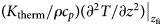 [°C s−1] determines the amount of refreezing Δz [m w.e.] that can take place in each time step as follows:

where L refr is the latent heat of freezing [J kg−1] and Δt is the time step length [s].
Here, we implement refreezing onto the ice slab using an offline forward Euler scheme that solves the 1-D heat equation. This scheme provides a look-up table of SI formation as a function of time elapsed since the first time step at which meltwater percolated down to the ice slab, that is, entered the lateral flow domain. It models refreezing by assuming an ice slab thickness of 10 m, with an initial ice slab temperature gradient decreasing linearly from 0°C at the slab surface to −10°C at 2 m depth, and below that a constant temperature of −10°C to 10 m depth. This initial temperature gradient is broadly representative of in situ temperature profiles around the time when the snowpack becomes isothermal as a result of melting and vertical percolation.
We run the refreezing scheme under the assumption that liquid water is always available on the ice slab surface for refreezing. At each time step this yields the change in the ice slab temperature profile and the maximum amount of refreezing that can take place. During model runs that incorporate refreezing, we use this output to determine refreezing in each gridcell as a function of both the time elapsed since the cell's snowpack became isothermal and the amount of water available for refreezing. Meltwater that refreezes is removed from the water table, and any remaining meltwater percolates laterally.
Lateral meltwater flow
Darcy's law is an empirical equation describing the flow of a fluid through a porous medium. It relates the flow rate of the fluid to the hydraulic gradient:

where q is the specific discharge, sometimes also called Darcy velocity [m s−1], Q is the flow rate or total discharge [m3 s−1], dh/dx is the hydraulic gradient [m m−1], A is the area through which flow occurs [m2] and K is the hydraulic conductivity [m s−1].
The hydraulic head h is a measure of fluid potential, or otherwise said the liquid pressure above a certain datum. It is the sum of two components: the elevation head z and the pressure head Ψ. Given that we are dealing with a single fluid, water, in an unpressurised system (where gridcells are open to the atmosphere), the pressure head is constant everywhere and the fluid potential is solely a result of the water table height and topographical elevation. Consequently, the hydraulic head can be simplified to the elevation head z. The hydraulic gradient is the difference in hydraulic head over the length of the flow path, which in this case is the distance between adjacent gridcells.
The hydraulic conductivity K describes the ease with which a fluid can move through a porous medium. It depends on the intrinsic permeability of the medium, the degree of fluid saturation, and the density and viscosity of the fluid, and is defined as

with k being the matrix permeability [m2], and ρ and μ the density [kg m−3] and dynamic viscosity of the fluid [Pa s].
Assessing model sensitivity
To determine the sensitivity of the model to the main input parameters, we conducted a sensitivity study using a model transect with a linear slope between 1900 and 1700 m a.s.l. We focused on three parameters with considerable uncertainty: hydraulic conductivity K, irreducible water saturation S w,irr and initial snowpack height h t=0. Other input parameters, such as snowpack porosity, ice slab temperature gradient and surface slope either exert a smaller influence on the modelling results, or manifest their impact on the simulation indirectly through the selected modelling approach for the empirically driven model runs.
Table 2 shows the low, base and high case values for the three tested parameters. For K, the chosen low and high case estimates correspond to the minimum and maximum observed lateral flow velocities in Clerx and others (Reference Clerx2022) divided by the slope of the study area, as the base assumption considers their average measured velocity. Further examination of why these values were chosen and how uncertain K is can be found in the discussion.
Low, base and high case values of parameters used for sensitivity analysis

The base case of S w,irr was set to 2% of the pore volume, which roughly equals 0.01 of the total volume, the minimum observed value by Denoth (Reference Denoth1982). This value was chosen as to limit the impact of this parameter on lateral meltwater flow in the model, resulting in this parameter only having a base- and high case in the sensitivity study. The high case value for S w,irr was set to 15% pore volume, or ~0.07 of the total volume, which is the highest value measured by Denoth (Reference Denoth1982) in a snow type that is still somewhat similar to the observed slush matrix.
Considering the initial snowpack height h t=0, the base case assumption of 1 m w.e. for the simulations over a linear slope is an overestimation of the annual accumulation in the study area. However, this choice was deliberate, as the main purpose of the model is to evaluate water table evolution over time, as well as over substantial lateral distances. A lower initial snowpack height would lead to very short simulations, since meltwater would appear at the surface as a result of the complete snowpack melting away after only limited amounts of melt. This would render the modelling results less useful, as meltwater runoff generally occurs throughout prolonged periods and not only in the early summer months. For sensitivity testing, the low case initial snowpack height corresponds to the average annual accumulation around KAN$\_$ U, whereas the high case value was set to 2.0 m w.e. We are aware that a snowpack this thick would typically lead to firn aquifer development instead of ice slab formation (MacFerrin and others, Reference MacFerrin2019), but this value was chosen to test the model.
We calculated three metrics to assess the model's sensitivity to changing these parameters. (1) Normalised discharge [m w.e.] corresponds to the total discharge (meltwater leaving the bottommost gridcell) divided by the average total generated meltwater per gridcell in each model run, and hence provides information about how much water leaves the modelled transect throughout the model run relative to melt input. (2) Simulation length describes the number of days before the water table completely saturates the snowpack in any one of the gridcells. (3) SI formation is the average volume of water [m w.e.] that is refrozen onto the ice slab in each gridcell along the model transect throughout the complete duration of the model run.
Results
Model sensitivity
Figure 3 shows three tornado plots that depict variations from the base case when using different values for hydraulic conductivity, irreducible water saturation and initial snowpack height for each of these metrics. Hydraulic conductivity K has a relatively symmetrical effect on how much water leaves the model (Fig. 3a). The influence of irreducible water saturation S w,irr is very limited, whereas variations in initial snowpack height have a positive impact for the warm melt seasons 2012 and 2019, in particular for the latter year.
Tornado plots showing model sensitivity to hydraulic conductivity, irreducible water saturation and snowpack height, displayed by variations in (a) normalised discharge, (b) simulation length and (c) average SI per gridcell at the end of each simulation. Hashed bars indicate the effect of using the high case of each tested variable, solid bars show the results when using the variable's low case.

In 2012, an extreme melt event late June was so intense that even a 2 m w.e. thick snowpack melts sufficiently for the water table to reach the snow surface early in the melt season, whereas the melting away of the complete snowpack occurs later in the more gradually developing 2019 melt season, allowing for a higher normalised discharge. For the two colder melt seasons 2017 and 2019, the low case initial snowpack thickness reduces the normalised discharge as a result of less available snow that can melt to subsequently runoff laterally. The model simulation length (Fig. 3b) is predominantly influenced by the initial snowpack height: despite the relatively high lateral meltwater flow velocities, the amount of snowpack available to accommodate melt is the most important parameter determining when water occurs at the snow surface. The amount of SI formation (Fig. 3c) represents the amount of meltwater retention and shows that the relatively conservative value for S w,irr could result in underestimation of SI formation. Initial snowpack height is once again the most influential parameter, and variations in K have less impact on the amount of SI formed.
The results of the sensitivity study underline the importance of carefully selecting the base case values, and reveal that certain parameters, notably initial snowpack height, have a pronounced impact on the model results.
Simulations along a linear slope
Figure 4 shows the evolution of water table height on top of the ice slab (a and b), snowpack height (c) and SI formation (d) during the 2020 melt season along a transect from 1900 to 1700 m a.s.l. with a linear slope, ~29 km in length. Panels (a) and (b) illustrate that the maximum water table height reached during the summer of 2020 was determined principally by the amount of melt input, and that SI formation plays a minor role. When comparing panels (a) and (b), two effects of SI formation are visible. Firstly, SI formation leads to a reduction in the maximum water table height (0.41 vs 0.35 m w.e. early August), and secondly it curtails the build-up of a water table at higher elevations, resulting in a diminished volume of liquid water present at the end of the melt season (maximum water table height of 0.33 vs 0.23 m w.e. end of September). Moreover, liquid water persists shorter and further upslope at the end of the melt season when SI formation occurs, indicated by the presence of water from ~15 km along the transect onwards in (b), whereas the water table is present below ~13 km in (a) at the end of September.
Water table evolution for the 2020 model runs (a) excluding and (b) including surface lowering and SI formation. Every coloured line represents the water table height at a weekly interval after the initial occurrence of water in the lateral flow domain. For the latter scenario snowpack height (c) and cumulative SI formation (d) are shown for a gridcell at 14.3 km along the transect, at 1800 m a.s.l.

Figure 5 shows characteristics of the simulation results for all of the four selected melt seasons, along the same transect as used for Figure 4. We computed normalised discharge and SI volume as fractions of the total available meltwater per gridcell in each model run at the end of the simulation. Given that some simulations do not run until the end of the simulation period (1 October) because the slush limit appears throughout the melt season, the absolute volume of meltwater discharge or water retained as SI cannot be compared quantitatively. The normalised values given here hence provide a way of removing the impact of the varying simulation lengths, as they only take into account the quantity of meltwater that was available during the model run, and not the total amount of melt throughout the whole melt season.
Simulation results for modelling runs along a transect with a constant slope between 1900 and 1700 m a.s.l. for four different melt seasons. SL and SI stand for surface lowering (due to melt) and superimposed ice formation, respectively. Panel (a) shows normalised discharge, with bar labels indicating the water breakthrough date (i.e. simulation length). In panel (b), the maximum water table height attained during the model run is displayed. Panel (c) shows the maximum height of SI formed in individual gridcells, and panel (d) displays the total amount of SI formed along the full model transect as a percentage of the total meltwater available in the whole model run.

Results show that water surfaced early in the season for 2012 and in two out of three cases for 2019, as a result of the high amount of meltwater input in these years. Although the total cumulative melt in 2019 was <1 m w.e., the visible runoff limit appeared around end of July. In 2012, this amount of melt was already reached before mid-July (see also Fig. 2), accompanied by meltwater appearing at the surface before the end of June.
The earlier in the melt season the water breakthrough, the more water is still present in the system, due to the fact that there has been less time for evacuating water by lateral runoff. This is shown by the lower values for normalised discharge in 2012 than in 2019 when looking at cases without SI formation. Much of this water presumably continues to drain out of the slush and into river channels which incise headwards after meltwater breakthrough, but simulating surface meltwater runoff is not included in the current modelling set-up.
Surface lowering has a stronger effect on the occurrence of the visible runoff limit than SI formation: the amounts of SI formed are an order of magnitude smaller than the surface height reduction by melt (e.g. 0.05 vs 0.5 m w.e. for 2019; Figs 5b, c). SI formation can, however, reduce the total amount of runoff by up to almost half: in 2012, normalised discharge is reduced to 6% with SI formation vs 10% without SI formation (Fig. 5a).
Simulations along the K-transect
Figure 6 shows the water table height (solid lines) and snowpack thickness (dashed lines) for the 2019 (warm; panel a) and 2020 (cold; panel b) melt seasons along a transect with the actual surface slope around the weather station KAN$\_$ U following the ArcticDEM, for the case where both surface lowering and SI formation were applied. Note the significant scale difference between the x- and y-axis in Figure 6c: the x-axis shows the horizontal distance of almost 30 km, whereas the y-axis displays the total elevation difference which is only 200 m. The initial snowpack height for these model runs was a more realistic 0.5 m w.e. as opposed to the 1 m w.e. initial snow thickness for the reference runs described in the previous section. Logically, reducing the snowpack thickness to 0.5 m w.e. has a significant impact on the model run duration: the water table now reaches the surface in all model runs except for the simulation for 2017 along the 1900–1800 m a.s.l. transect (Fig. 7a).
Evolution of water table (solid) and snowpack (dashed) height over time for 2019 (a) and 2020 (b) with surface lowering and SI formation, and (c) gridcell height and slope gradient along the transect. Every coloured line represents a weekly interval after the initial occurrence of water in the lateral flow domain. Absent lines in 2019 (a) are a result of the simulation being stopped due to earlier water breakthrough than in 2020. Note the small area of zero-slope ~9 km along the transect.

Simulation results for modelling runs along the K-transect slope between 1900–1700 and 1900–1800 m a.s.l. for four different melt seasons, with surface lowering due to melt and SI formation. Panel (a) shows the elevation and date at which meltwater appears at the surface. In panel (b), the maximum simulated water table height reached is shown. Panel (c) displays the maximum height of SI formed throughout the melt season. Panels (d) and (e) show the total amount of discharge and SI formation as a percentage of the total meltwater available in the whole model run.

Changes in transect gradient have an important effect on the water table height. Both in Figures 6a, b it can be seen that at 2 km, just before 9 km and ~14 and 23 km water accumulates due to a slope decrease, whereas at 9, 17 km and just after 20 km water is evacuated more efficiently, demonstrated by a local decrease in water table height related to an increase in slope.
Especially in 2020 (Fig. 6b) the effect of lateral meltwater flow is clearly visible by the downslope migration over time of the highest water table below 2 and 22 km, where the transect slope decreases. Similarly, in 2019 (Fig. 6a) the water table peak ~2 km moves slightly downslope after a short pause in meltwater supply between the 1st and 8th of July.
Figure 7 shows the results for the simulations along the K-transect slope displayed in Figure 6c for all studied melt seasons, for a transect between 1900 and 1800 m a.s.l. (green bars) and for the transect spanning the full elevation range (1900–1700 m a.s.l.; purple bars) to investigate the impact of less melt at higher elevations. In all these model runs the initial snowpack height was 0.5 m w.e.
As shown in Fig. 7a, both transects have a specific elevation for water breakthrough at the surface, regardless of its timing, corresponding to an inflection point in surface slope. In general, the maximum water table reached is slightly higher for the shorter (1900–1800 m a.s.l.) transect (Fig. 7b). Similarly, when only looking at the upper part of the transect (green bars), there is 2–5% more accretion of SI in individual gridcells than when considering the 1900–1700 m a.s.l. elevation range (purple bars; Fig. 7c). The discharge as a function of total meltwater available during the model run (Fig. 7d) is substantially higher for the shorter model transect (green bars). These results are primarily a function of the model's longer runtime before the visible runoff limit appears in case of the model runs using the longer 1900–1700 m a.s.l. transect. The total thickness of newly formed SI as a function of the amount of meltwater available throughout the whole melt season is similar across the two transect variations (Fig. 7e).
Discussion
Timing and location of slush appearance
As shown in the sensitivity analysis (Fig. 3), initial snowpack height plays an important role in the timing of slush appearance at the surface, even within the relatively narrow range of minimum and maximum values. The chosen initial snowpack height for a linear slope exceeds measured values along the K-transect, but using more realistic, lower values reduces model utility as water breakthrough occurs earlier, stopping the model run.
The increase in water table height over time on top of an ice slab is dependent on the evolution of the melt season throughout the summer. Shorter, intense periods of melt are more likely to cause the appearance of visible runoff than more gradual meltwater supply, as shorter periods allow for less lateral flow through the firn evacuating the meltwater downslope.
In general, the occurrence of visible runoff takes place later in the melt season at higher elevations according to the results for the two modelled elevation intervals (Fig. 7a): simulations using the longer 1900–1700 m a.s.l. transect (purple markers) result in earlier occurrence of the slush limit than on the shorter transect. This is a result of the lower amount of melt at higher elevations, as well as the impact of lateral meltwater supply. For 2012 and 2020 there is relatively little difference in timing between the two elevation ranges due to the rather abrupt, large melt events taking place towards the end of June in 2012 and late-July in 2020, but for 2017 and 2019 there are significant delays in slush limit occurrence between the transect from 1900 to 1800 m a.s.l. when compared to 1800–1700 m a.s.l. results. Abrupt and strong melting seems to lead to flooding of the snowpack over substantial elevation intervals, whereas sustained, moderate melt does not have this effect.
In colder summers, when the simulated water table does not reach the snow surface, differences in the total amount of discharge and SI formation are principally due to differences in temporal evolution and the total quantity of meltwater generated during the melt season. For example, in 2017 more SI was formed because of a more gradual evolution of the melt season, whereas in 2020, when a big melt event occurred in late-July, a larger part of the supplied meltwater ran off. Apart from the higher absolute amount of liquid water available in 2020, there was less time for refreezing that year due to the sudden input of melt and subsequent faster lateral meltwater displacement as a result of higher hydraulic gradients.
When comparing the characteristics of the linear model runs to those of the runs with a varying slope along the K-transect, it can be seen that the influence of slope variations is larger than that of surface lowering: for the same melt input, the water table reached higher levels more rapidly when the transect followed a non-linear slope (Figs 5a and 7a, purple markers). In the simulations with a linear slope, the maximum water table attained at the end of the simulations was approximately half the initial snowpack height of 1 m w.e. but smaller in most cases (Fig. 5b). For the model runs using the K-transect slope, the maximum water table height at the time of water breakthrough was ~0.6× the initial snowpack height of 0.5 m w.e (Fig. 7b). Across all simulations along the K-transect elevation profile, meltwater first occurred at locations characterised by a decrease in slope. This is particularly pronounced during colder summers with a gradual supply of meltwater, when lateral flow is of even greater relative importance for total runoff than when short-lived, intense melting provides the majority of liquid water. Changes in ice slab slope, or more broadly in surface slope, therefore play a major role in the occurrence of the visible runoff limit.
Our results corroborate with the findings on the daily variation of visible runoff limits by Machguth and others (Reference Machguth, Tedstone and Mattea2022) for the four melt seasons studied here. In particular in the simulations for the 100 m elevation transect (Fig. 7a, green markers), the timing of meltwater appearing at the surface roughly corresponds to when the maximum visible runoff limit was observed on satellite imagery. However, a comprehensive comparison with field observations remains challenging due to the simple nature of the lateral flow model. In the current model configuration, meltwater is only transported downslope, and each gridcell can only receive meltwater input from its upslope neighbour. In reality, flowpaths are a function of the surface hydrological catchment, so a given point in space could receive meltwater input from several directions.
At present, simulations are stopped as soon as the water table height reaches the snow surface in any of the gridcells, since surface meltwater runoff is not included in the model. This is the most obvious (or only physically realistic) end for a model run currently. We have only very limited knowledge on how fast water flows in visible slush fields, or how these develop into efficient supraglacial drainage systems (e.g. Holmes, Reference Holmes1955). From satellite imagery it is clear that, after a certain period of time with sufficient and sustained melt, slush fields nearly always transition into more confined supraglacial river systems. Given the efficiency of this process – based on remote-sensing data we can observe that the development of efficient surface drainage systems is a matter of days rather than weeks – including a simplistic bucket scheme in the model for surface runoff would probably be a valid approximation. This would avoid the necessity of incorporating a full 2-D-meltwater routing scheme with all related assumptions and uncertainties. Ideally, the model should always run until the end of the melt season regardless of the amount of melt to allow for adequate comparison between individual melt seasons. Including surface runoff, even in the form of a simplistic bucket scheme, would allow simulations to run for the full melt season.
Lateral meltwater runoff and hydraulic properties
Lateral meltwater runoff is highly efficient in all model simulations. For any gridcell except for the uppermost along the transect, runoff greatly exceeds the amount of vertical surface meltwater input due to the large lateral inflow from higher elevations. Depending on the temporal evolution of the melt season, total lateral runoff (i.e. the total amount of lateral outflow in an individual gridcell for the complete simulation duration) is ~40 times the meltwater input from local melt in individual gridcells at the time the water table reaches the snow surface. Note that total lateral runoff is different from the total discharge, which we define as the total volume of lateral meltwater outflow of the bottommost gridcell along the modelled transect. The amount of lateral runoff as a function of average total meltwater generated in gridcell is higher for the 1900–1800 m a.s.l. transect than for the transect spanning a 200 m-elevation range (56× vs 37× more runoff than melt input, respectively).
The model outcomes from the longer transect show lower values for the normalised discharge (Fig. 7d; green bars). This is due to the fact that it takes much longer for meltwater to exit the transect as the model grid is about twice as long as that of the transect spanning a 100 m elevation range.
The sensitivity study shows that the hydraulic conductivity has a large impact on the model results, in particular concerning the amount of meltwater discharge and retention. Measured hydraulic conductivities of firn at various glaciers across the world fall within a relatively narrow range, typically between 1×10⁻⁵ and 5×10⁻⁵ m s−1 (Fountain and Walder, Reference Fountain and Walder1998). However, in areas where firn aquifers exist, firn hydraulic conductivity measurements show a considerably wider range, spanning from 2.5 × 10⁻⁵ to 1.1 × 10⁻³ m s−1 (Miller and others, Reference Miller2017), and when including measurements of weathering crust hydraulic conductivity (3.47 × 10⁻⁸ to 4.07 × 10⁻⁵ m s−1) this range widens further (Stevens and others, Reference Stevens2018). In the southwest of Greenland, hydraulic conductivity of near-surface icy firn has been measured at 2.4 ± 1.0 × 10⁻³ m s−1 (Clerx and others, Reference Clerx2022).
When calculating the hydraulic conductivity of the slush matrix using the Kozeny–Carman approximation for permeability of a porous medium consisting of perfect spheres (Kozeny, Reference Kozeny1927; Carman, Reference Carman1937; Bear, Reference Bear1972), a more theoretical approach, using a porosity ϕ of 0.45, density ρ w of 1000 kg m−3 and viscosity μ of 1.7916 × 10⁻³ Pa s (for water at 0°C) yields a hydraulic conductivity of 3.67 × 10⁻² m s−1. Using Calonne's and Shimizu's parametrisations for snow permeability, respectively (Shimizu, Reference Shimizu1970; Calonne and others, Reference Calonne2012), in combination with the same parameters described for the Kozeny–Carman approximation, leads to theoretical values for hydraulic conductivity of 9.34 × 10⁻² and 3.30 × 10⁻² m s−1.
In our model calculations, the hydraulic conductivity parameter K (3.84 × 10⁻¹ m s−1, which is two orders of magnitude higher than values measured in the laboratory-type experiments using icy firn by Clerx and others, Reference Clerx2022) is derived from observed lateral flow velocities of meltwater through slush, and not a direct material property measurement.
All in all, in the various measurements and possible theoretical approaches there is a spread of several orders of magnitude and hence substantial uncertainty in the hydraulic conductivity of snow and firn, with theoretical approximations giving values that are approximately in the middle of the range, and hydraulic conductivities measured in the field providing both lower and higher values. The currently used value for K in the model based on the field observations by Clerx and others (Reference Clerx2022) was chosen in order to obtain modelling results that resemble in situ measurements of lateral meltwater flow. A lower hydraulic conductivity would lead to less runoff and a delay in occurrence of the visible runoff limit. For future model development, it is essential to better constrain the parameter space of potential hydraulic conductivity values by further in situ measurements of snow, firn and slush matrix hydraulic conductivity. Additionally, understanding how these values fluctuate throughout the melt season would be very valuable, as hydraulic conductivity is unlikely to remain constant as a result of meltwater processes and continued snow transformation.
The irreducible water saturation S w,irr is set to a relatively low value of 2% of the pore volume (~0.01 of the total volume) in our simulations, to reduce the importance of the vertical flow domain in the model. We do not have detailed insights into the actual residual water saturation in slush on top of ice slabs. Furthermore, considerable uncertainty remains in general as to what is a representative value for the irreducible water saturation in snow. Dielectric measurements (Lemmelä and Kuusisto, Reference Lemmelä and Kuusisto1974) show irreducible water saturations of 0.02–0.03 for a seasonal snowpack, whereas Coléou and Lesaffre (Reference Coléou and Lesaffre1998) measured values for wet snow between 0.05 and 0.15 in a laboratory setting. We consider the lowest value for S w,irr as reasonable, given the relatively high percolation- and lateral flow velocities compared to the model time step, but also since large areas can undergo the transformation into slush fields within several days. Given the sensitivity of the ratio between meltwater runoff and retention (normalised discharge and SI formation in the sensitivity study) to irreducible water saturation, deliberate choices and further analysis of the most appropriate base case value for S w,irr should be made when developing the lateral flow model further.
Refreezing
SI formation can account for meltwater retention of up to 40%, especially at high elevations (Fig. 7e). In case of intermittent melt pulses this can drastically delay or even completely inhibit the occurrence of visible water at the surface. Values for total thickness of newly formed SI as a function of total available meltwater are slightly higher for the upper (short) K-transect model runs as melt is slightly less at higher altitudes, resulting in a somewhat larger fraction of meltwater retention.
Simulated values for SI formation on top of the ice slab (0.02–0.13 m w.e.) are in broad agreement with data from Rennermalm and others (Reference Rennermalm2021) which allow evaluating ice slab growth at KAN$\_$ U in consecutive years. Their firn cores yield values in the order of 0.3–0.4 m accretion of ice slab thickness per year (~1.6 m ice in 5 years, or 0.28–0.37 m w.e. a−1). The lower ice accumulation in the model is presumably a result of its 1-D nature only considering meltwater inflow from one direction, whereas in reality more water can accumulate due to local ice slab topography and resulting meltwater ponding.
In the current model configuration, refreezing only takes place in the lateral flow domain. This is a simplification, as we know from literature and field observations that ice lenses and glands form in the percolation domain (e.g. Baird, Reference Baird1952; Koerner, Reference Koerner1970; Mikhalenko, Reference Mikhalenko1989; Obleitner and Lehning, Reference Obleitner and Lehning2004; Parry and others, Reference Parry2007; Cox and others, Reference Cox, Humphrey and Harper2015), but deemed appropriate given the model simplicity and purpose. In other regions of the Greenland ice sheet, where crevasses and fractures are more common than in our study area, crevassing can increase the effective permeability enough to restrict lateral meltwater flow and runoff, hence enabling enhanced refreezing of meltwater that vertically percolates to depth (Culberg and others, Reference Culberg, Chu and Schroeder2022). Additionally, refreezing can also occur from above (i.e. at the snow surface) and not only in the form of SI that accretes to the top of the ice slab.
At the start of all the model runs on 1st April, we assume that the full snowpack on top of the ice slab is isothermal at 0°C, as we do not simulate the initial warming of the snowpack in the beginning of the melt season. Additionally, we do not model the vertical percolation domain in detail. In years characterised by low amounts of melt, this simplification does not fully capture refreezing processes, especially regarding the formation of ice lenses and intermediate refreezing that may have an impact on the flow properties of the snowpack. These assumptions hence may lead to an overestimation of SI formation in our model. However, the applied initial ice slab temperature gradient, where ice slab temperature decreases linearly from 0 to −10°C between 0 and 2 m depth and only remains constant at −10°C below 2 m depth, implies that a certain amount of warming has already taken place before the onset of the melt season. Field measurements of firn temperature (e.g. Humphrey and others, Reference Humphrey, Harper and Pfeffer2012; Machguth and others, Reference Machguth2016; MacFerrin and others, Reference MacFerrin, Stevens, Vandecrux, Waddington and Abdalati2023) show that this a realistic assumption to account for and average out yearly and shorter-term variations in ice slab temperature.
Conclusions
We designed a simple, physics-based quasi-2-D model to describe lateral meltwater flow and SI formation atop near-surface ice slabs. The model was used to simulate four melt summers in the southwest of the Greenland ice sheet, and provides the development of water table- and snowpack height throughout the melt season, as well as values for the total amount of total discharge and meltwater retention in the form of newly formed SI.
Our results show that the evolution of the water table height and the occurrence or absence of a visible runoff limit is very dependent on the evolution and intensity of individual melt seasons. In general, less melt at higher altitudes leads to the later occurrence or absence of meltwater at the surface, although even in relatively colder melt seasons the water table can appear at the snow surface in case of short, intense melt events.
Changes in surface gradient play a major role in the appearance of the visible runoff limit. Modelling results imply localised areas of slush formation in areas where the surface slope is flatter, which corresponds to observations made in the field and on satellite imagery.
Lateral flow is a very efficient mechanism for meltwater runoff: in most model gridcells lateral outflow is more than 30× larger than the amount of meltwater generated in situ. Measurements of snow and firn hydraulic properties exist, yet given the wide range of values provided by field observations, in particular the hydraulic conductivity remains a source of uncertainty in the model.
SI formation can account for up to 40% of meltwater retention, and especially in case of intermittent melt pulses this can drastically delay the occurrence of visible meltwater at the surface. Values of modelled total SI formed (0.02–0.13 m w.e. throughout part of the melt season) roughly match observations of ice slab thickening at KAN$\_$ U (0.28–0.37 m w.e. accretion of ice slab thickness per year).
In summary, our study highlights the pivotal role of lateral flow as a mechanism driving surface meltwater runoff. However, despite the insights gained from our simplified model, direct comparison with field- or remote sensing data remains challenging. The complex nature of the hydrological processes at play makes validation of results non-trivial. Efforts to enhance and expand the 1-D-model are required and ongoing, but the results presented in this paper are a first step towards a more comprehensive understanding and description of the hydrological system in the accumulation zone of the southwestern Greenland ice sheet.
Data
A description of the required input data, the input data that was used for the modelling as well as the full model code are available at https://doi.org/doi.org/10.5281/zenodo.13866141.
Acknowledgements
This study is funded by the European Research Council (ERC) under the European Union's Horizon 2020 research and innovation programme (project acronym CASSANDRA, grant agreement No. 818994). We sincerely thank Bettina Schaefli and Nander Wever for their input and advice while shaping the model design and strategy.
Author contributions
H. M. and N. C. designed the study with contributions from A. T. N. C. programmed the model with contributions from H. M. and input data provided by D. v. A. N. C. carried out the model simulations and prepared the manuscript with contributions from H. M., A. T. and D. v. A.


 Open access