2.1.1 Sources of reionisation

The 21-cm sky contains a wealth of information about the properties of the ionising sources because they strongly affect the topology of the EoR. Reionisation scenarios dominated by stars in galaxies produce well-defined ionised regions, while ‘miniquasars’ (small accreting black holes) yield more diffuse features (Zaroubi & Silk Reference Zaroubi and Silk2005) and reionisation processes involving decaying/annihilating dark matter particles would be very inhomogeneous (Belikov & Hooper Reference Belikov and Hooper2009). The 21-cm observations could even distinguish between different stellar reionisation scenarios (Lidz et al. Reference Lidz, Zahn, McQuinn, Zaldarriaga and Hernquist2008). For example, more massive galaxies produce larger ionised regions (Furlanetto, Zaldarriaga, & Hernquist Reference Furlanetto, Zaldarriaga and Hernquist2004; McQuinn et al. Reference McQuinn, Lidz, Zahn, Dutta, Hernquist and Zaldarriaga2007). If it is able to constrain the shape and evolution of the power spectrum, the MWA will reveal the nature of some of the first cosmological objects.

2.1.2 The neutral fraction

Existing observations have provided tantalising hints about reionisation, but even more unanswered questions. CMB observations find that the average redshift of reionisation is z = 10 ± 2 (Komatsu et al. Reference Komatsu2009), and quasar absorption spectra imply that the Universe was totally ionised by z = 6, one billion years after the big bang. In addition, several studies have interpreted the large saturated regions at z > 6 in these absorption spectra as evidence for the end of reionisation (e.g. Fan et al. Reference Fan2006), but this conclusion is disputed (Becker, Rauch, & Sargent Reference Becker, Rauch and Sargent2007; Mesinger Reference Mesinger2010).

Detection of the 21-cm power spectrum will yield measures of x _Hi(z) through predictable features that depend on the neutral fraction. As evident in Figure 3, the intensity of 10 cMpc scale fluctuations in 21-cm brightness temperature briefly fades when reionisation begins and the first galaxies ionise the overdense regions within a couple of cMpc of them. Next, the ionised regions surrounding individual galaxies overlap, creating ~10 cMpc ionised regions and an increase in power on these scales. Finally, all of the fluctuations fade as these bubbles overlap, swallowing the neutral hydrogen that remains. Each of these trends can be used to disentangle x _Hi(z).

For many possible sources that have been considered in the literature (such as galaxies, quasars, and mini-halos), the amplitude of the power spectrum peaks at x _Hi ≈ 50%. The MWA could probe the global ionisation history by tracking the evolution of this amplitude and shape of the 21-cm power spectrum. Using these features, the volume-filling factor of neutral hydrogen (comparable to the mass-averaged neutral fraction) can be constrained after approximately two years of observations to between 0.4<x _HI<0.75 at 2σ significance for the redshift where the power spectrum achieves its maximum amplitude (Lidz et al. Reference Lidz, Zahn, McQuinn, Zaldarriaga and Hernquist2008). While unlikely, it is possible that the IGM is highly ionised over the range of redshifts measured by the MWA. Lidz et al. (Reference Lidz, Zahn, McQuinn, Zaldarriaga and Hernquist2008) found that a null detection with the MWA at z ≤ 8 would be able to constrain the neutral fraction to ≲4%.

Observations of individual quasar H ii regions offer an additional probe of the global neutral hydrogen fraction since the contrast between the ionised H ii region and neutral IGM can provide a measurement of the neutral fraction at the redshift of the quasar. Geil et al. (Reference Geil, Wyithe, Petrovic and Oh2008) have found that the shape of the quasar H ii regions can be recovered from foreground subtracted MWA maps by using the entire data cube to help determine the contrast between the external IGM and ionised interior.

2.4.1 Reference pipeline

The baseline foreground subtraction strategy is a multi-stage process consisting of the following principal stages:

1. Bright source subtraction. The first step in foreground subtraction is the removal of bright points sources. This is necessary because the sidelobes of these sources mask the 21-cm signal. Recent theoretical studies have indicated that bright point source subtraction must be complete for sources with flux greater than S ≳ 100 mJy in order to allow for successful subsequent Galactic continuum foreground subtraction (Liu, Tegmark, & Zaldarriaga Reference Liu, Tegmark, Bowman, Hewitt and Zaldarriaga2009). The brightest sources in the field will be ‘peeled’ (self-calibrate and subtract) from the raw visibility measurements (Mitchell et al. Reference Mitchell, Greenhill, Wayth, Sault, Lonsdale, Cappallo, Morales and Ord2008). Efficient techniques to remove point sources from gridded and integrated maps are also under investigation (Pindor et al. Reference Pindor, Wyithe, Mitchell, Ord, Wayth and Greenhill2011; Bernardi et al. Reference Bernardi, Mitchell, Ord, Greenhill, Pindor, Wayth and Wyithe2011).

2. Diffuse continuum subtraction. A variety of mechanisms contribute to diffuse continuum emission in the low-frequency radio sky including Galactic synchrotron emission, Galactic free–free emission, extragalactic free–free emission, and a sea of faint extragalactic point sources that are too numerous to identify individually in maps and are, thus, said to be ‘confused’. All of these foregrounds are significantly stronger than the redshifted 21-cm signal and have considerable angular structure on the sky (see Figure 2; Santos, Cooray, & Knox Reference Santos, Cooray and Knox2005, their Figure 5). But the emission mechanisms of these foregrounds produce smooth spectra that follow power-law profiles, making them possible to separate from the redshifted 21-cm emission by their long spectral coherence scales compared with the small, ~1-MHz spectral coherence of the reionisation signal. A variety of techniques have been proposed to accomplish this separation including polynomial fits along the spectral axis of each pixel in an image map or its uv-map conjugate, Minkowsky functionals, and non-parametric techniques. The baseline approach planned for the MWA is to fit and subtract a third-order polynomial from each pixel in the uv-domain representations of the bright source cleaned maps. This technique has been demonstrated for the MWA in the limit of perfect instrumental calibration (Liu et al. Reference Liu, Tegmark, Bowman, Hewitt and Zaldarriaga2009a; Bowman, Morales, & Hewitt Reference Bowman, Morales and Hewitt2009; Liu et al. Reference Liu, Tegmark, Bowman, Hewitt and Zaldarriaga2009b).

Figure 5.

Polarised intensity at Faraday depth zero at 189 MHz from the MWA development system (Bernardi et al. Reference Bernardi2013). The field spans 2 400 deg² with 15-arcmin angular resolution and is roughly centred on the southern Galactic pole, extending to within 20° of the Galactic plane. The radial lines are Galactic latitude and the circular arcs indicate Galactic longitude. Flux density is plotted on a linear colour scale from 0 to 0.2 Jy beam⁻¹ RMSF⁻¹ (white to black), where RMSF is the RM spread function. Polarised maps from the MWA showing similar complex structures and discontinuities that often have no counterparts in total intensity will be used to determine the properties of both ordered and turbulent magnetic fields in the Milky Way's ISM (see Figure 6).

3. Polarised leakage subtraction. In addition to the foreground issues discussed thus far, gain and phase calibration errors and non-ideal feeds conspire to contaminate all Stokes parameters further. This leakage leads to some portion of the complex linear polarisation signal finding its way into the Stokes I intensity maps that will be used for the redshifted 21-cm measurements. By using rotation measure (RM) synthesis (Brentjens & de Bruyn Reference Brentjens and de Bruyn2005; see also Section 3.3) to exploit the Fourier relationship between the polarised signal and the Faraday dispersion function, it is possible to identify components of the polarised signal with specific Faraday depth. The three-dimensional Stokes I data set is first re-sampled along the frequency axis into the natural λ²-basis for Faraday rotated emission. A one-dimensional Fourier transform is then applied along each line of sight. Any feature observed with a non-zero Faraday depth in the three-dimensional RM synthesis map will, by definition, be polarised contamination. By applying an inversion process together with knowledge of the instrument's specific leakage behaviour, this contamination can be subtracted (Geil, Gaensler, & Wyithe Reference Geil, Gaensler and Wyithe2011).

4. Statistical template fitting and power spectrum estimation. Many classes of errors and residuals remaining in the maps after the foreground cleaning stages described above can be modelled given sufficient knowledge of the instrumental response (Morales, Bowman, & Hewitt Reference Morales, Bowman and Hewitt2006; Bowman et al. Reference Bowman, Morales and Hewitt2009; Datta, Bowman, & Carilli Reference Datta, Bowman and Carilli2010; Morales et al. Reference Morales, Hazelton, Sullivan and Beardsley2012). The statistical properties of these residuals can be exploited to provide an additional layer of foreground removal by fitting templates of the residual statistical structures during the final redshifted 21-cm power spectrum parameter estimation. This technique is now commonly employed in CMB power spectrum analysis to account for the angular power of faint point sources and the effects of gravitational lensing.

2.4.2 Unified parameter estimation

The stages of foreground subtraction outlined above can be performed discretely, resulting in a series of output products, the last of which is used as the input into power spectrum estimation and other statistical tests to extract information from the redshifted 21-cm signal. Alternatively, they can be performed in a unified matrix framework that simultaneously fits models for the foreground contributions and the 21-cm statistical signal (Liu & Tegmark Reference Liu and Tegmark2011; Tegmark Reference Tegmark1997). The latter has the advantage of producing an optimal result that minimizes both bias (from thermal noise and foreground contamination) and correlations between parameters, and yields the smallest possible error bars, but at the expense of a large computational overhead. Advances in processing power and new efforts at sparse matrix reduction have begun to enable the trial application of unified parameter estimation in simulations and preliminary data, and it is expected this approach will ultimately be the preferred technique for data analysis.

4.1.1 Low-mass stars and brown dwarfs

Magnetised plasmas in stellar coronae (the outer layers of a star's magnetosphere) produce strong radio emission through non-thermal, collective, and/or coherent processes. This emission reflects local properties such as density and magnetic field strength and can be used to understand magnetic field generation, magnetospheric structure, angular momentum evolution, magnetic flaring mechanisms, and accretion processes. Furthermore, magnetic fields provide one of the few indirect probes of stellar interiors.

While radio studies of late-type stars and active binaries are well established (see Güdel Reference Güdel2002 for a review), radio observations of the lowest mass stars and brown dwarfs—objects incapable of sustained core hydrogen fusion (Kumar Reference Kumar1962)—have only recently been demonstrated and comprise a relatively new tool in this active field of research. M dwarfs with masses 0.1–0.5 M_⊙ are a dominant stellar component of the Galaxy, comprising ~70% of all stars. They are also known to exhibit high levels of magnetic activity, with strong surface magnetic fields (~2–4 kG, compared with ~10 G on the Sun; Saar & Linsky Reference Saar and Linsky1985; Johns-Krull & Valenti Reference Johns-Krull and Valenti1996) and substantial filling factors (50%–80% of the surfaces of M dwarfs are covered by magnetic fields; Johns-Krull & Valenti Reference Johns-Krull and Valenti1996). Magnetic radio emission from M dwarfs has been observed in many nearby systems, both flaring and quiescent, predominantly in the 1–10-GHz band. These studies have confirmed the existence of large-scale, organised magnetic fields around stars with fully convective interiors (Donati et al. Reference Donati, Forveille, Cameron, Barnes, Delfosse, Jardine and Valenti2006), despite the loss of the αΩ dynamo that powers the Solar field (Parker Reference Parker1955).

For even lower mass stars and brown dwarfs, the detection of both quiescent and flaring radio emission was initially a surprise (Berger et al. Reference Berger2001), as the flux from these sources is orders of magnitude greater than that expected from the Güdel–Benz relation.Footnote ⁵ Several late-type sources have now been detected at GHz frequencies (Figure 8), in many cases despite the absence of optical or X-ray emission (see Berger Reference Berger2006 for a review). Indeed, while Hα and X-ray luminosities relative to bolometric luminosities appear to decline with spectral type, relative radio emission inexorably increases up to the substellar regime (see Burgasser & Putman Reference Burgasser and Putman2005; Berger Reference Berger2006; Audard et al. Reference Audard, Osten, Brown, Briggs, Güdel, Hodges-Kluck and Gizis2007). Understanding why radio emission is so prominent among these very low mass objects, and whether such emission correlates with age, rotation, or other physical parameters, remain outstanding questions.

Figure 8.

Phase space for radio transients observable with the MWA at a nominal frequency of 200 MHz, updated and adapted from Cordes et al. (Reference Cordes, Lazio and McLaughlin2004). We plot the product of the observed peak flux density S _peak and the square of the distance D ² (like a luminosity) against the product of the emission frequency ν and the transient duration W. In the Rayleigh–Jeans approximation, these quantities are directly proportional and related to the brightness temperature T (given by the diagonal lines); we use a brightness temperature of 10¹² K (thick diagonal line) to divide coherent and incoherent processes (Readhead Reference Readhead1994). The red lines show the predicted sensitivity of the MWA, assuming a 50-mJy source can be detected in 8 s. The vertical red lines give the timescales for individual snapshot observations (8 s), and short- and long-term surveys (5 m and 1 week). The red diagonal lines give the S _peak D ² limits corresponding to distances of 10 pc (appropriate for sources such as low-mass stars, brown dwarfs, and planets), 1 kpc (local Galactic sources), 10 kpc (the Galactic Center), 1 Mpc (local group), and 1 Gpc (extragalactic sources); the dotted lines show an estimated confusion limit of 10 mJy, although we can search below this limit using image subtraction or for polarised emission.

Radio flares in particular demonstrate that this emission is associated with magnetic events, occurring over timescales of microseconds to minutes (e.g. Osten & Bastian Reference Osten and Bastian2006). The brightness temperatures of bursting emissions frequently exceed 10⁹ K, indicating coherent processes as confirmed by high circular polarisations (30%–100%). Yet, radio variability from these sources is remarkably diverse, from strong (30-mJy peak flux), narrowband, fully polarised, bursting emission with frequency drifts (Burgasser & Putman Reference Burgasser and Putman2005), to periodic bursts suggestive of pulsar-like beaming (Hallinan et al. Reference Hallinan2007, and Figure 8), to order-of-magnitude variations spanning years (Antonova et al. Reference Antonova, Doyle, Hallinan, Golden and Koen2007). It has even been suggested that the observed ‘quiescent’ emission from these sources may be the result of low-level, sustained electron cyclotron maser emission (e.g. Hallinan et al. Reference Hallinan2007). The physical origin of transient radio bursts from low-mass stars, their incidence rates (duty cycle estimates range from 1%–30%), and their spectral characteristics are either poorly constrained or entirely unknown. These questions have a direct impact on whether low-mass stars comprise a significant fraction of radio transients in general (e.g. Kulkarni & Phinney Reference Kulkarni and Phinney2005; Kaplan et al. Reference Kaplan, Hyman, Roy, Bandyopadhyay, Chakrabarty, Kassim, Lazio and Ray2008).

The MWA has the potential to contribute substantially to our understanding of both quiescent and flaring magnetic emission from low-mass stars and brown dwarfs. By sampling the 80–300-MHz band, MWA observations can be used to constrain the peak frequency (ν_pk) and spectral indices about ν_pk, enabling the determination of coronal field strengths (currently estimated at 10–100 G; Burgasser & Putman Reference Burgasser and Putman2005; Berger Reference Berger2006), electron densities and the fundamental nature of the emission. Audard et al. (Reference Audard, Osten, Brown, Briggs, Güdel, Hodges-Kluck and Gizis2007) argue that radio emission from very low mass stars may in fact peak in the ~100-MHz range if it arises from electron cyclotron emission from weak fields (ν_pk = ν_c = 30–300 MHz for 10–100-G fields; see also Osten et al. Reference Osten, Hawley, Bastian and Reid2006). The sensitivity of the MWA is essential for this work, given the intrinsic faintness, but variable nature, of radio emission from low-mass stars; estimates range over 10 μJy to 100 mJy at 100 MHz at a distance of 10 pc, depending on the emission mechanism. Similarly, the MWA's wide-field capabilities are necessary to build up statistically robust samples, particularly given the roughly uniform distribution of nearby low-mass stars in the vicinity of the Sun. High spectral resolution observations enabled by the MWA will permit studies of field dynamics and remote determinations of physical parameters such as the heights of magnetic reconnection regions, electron speeds, and the density profile of the stellar coronae.

4.1.2 Magnetars

While a variety of neutron stars can produce transient or steady radio emission (discussed in more detail in Section 4.4), some subclasses of neutron stars can give rise to extremely energetic, explosive phenomena. With magnetic fields of ~10¹⁵ G, magnetars (Duncan & Thompson Reference Duncan and Thompson1992; Thompson & Duncan Reference Thompson and Duncan1995) undergo catastrophic reconnection events known as ‘giant flares’ that release >10⁴³ erg. With each flare the magnetars release blobs of relativistic plasma (Frail, Kulkarni, & Bloom Reference Frail, Kulkarni and Bloom1999; Gaensler et al. Reference Gaensler2005b; Cameron et al. Reference Cameron2005) with peak fluxes of hundreds of mJy at frequencies from 200 MHz up to 100 GHz (Figure 8). Such events are detected through high-energy satellites, but the radio monitoring provides vital diagnostics of the flare properties and energetics.

Beyond this, some magnetars unexpectedly have steady radio emission that is modulated at the X-ray pulse period (2–12 s). Prior searches for steady-state radio emission from magnetars had not been successful (e.g. Kaplan et al. Reference Kaplan, Kulkarni, Frail and van Kerkwijk2002), but Halpern et al. (Reference Halpern, Gotthelf, Becker, Helfand and White2005) found a radio source coincident with the magnetar XTE J1810–197 (also Camilo et al. Reference Camilo, Ransom, Halpern, Reynolds, Helfand, Zimmerman and Sarkissian2006, and others). Monitoring the magnetars through both individual pulses and phase-averaged emission, looking for both giant flares and the onset of bright phases, will help understand the duty cycles of the radio-bright phases and hence unravel the puzzles that they present.

4.1.3 X-ray binaries

Relativistic outflows or jets are a widespread yet transient consequence of accretion onto compact objects. Radio jets are seen for black-hole binaries (BHBs) and some neutron-star binaries (NSBs). These sources are collectively called ‘microquasars’ (Figure 8), since they exhibit scaled-down and rapidly evolving versions of the jets in active galactic nuclei. Microquasars exhibit several types of jets with different ranges of radio power and ejection timescale. Their study is crucially dependent on the correlated variations in radio and X-ray properties.

The most common type of jet in microquasars is the quasi-steady jets associated with the X-ray hard state (Fender, Belloni, & Gallo Reference Fender, Belloni and Gallo2004; McClintock & Remillard 2006) that can persist for months in some sources. Steady jets are estimated to be mildly relativistic (i.e. ~0.7c; see Fender Reference Fender, Lewin and van der Klis2006), but there is uncertainty about the baryonic content and hence the scale of the mass outflow and the fraction of accretion energy needed to power such jets.

Impulsive ejections are also produced by BHBs and some NSBs and the brightest of these are seen as bipolar radio jets that move with velocities as high as 0.98c (Mirabel & Rodríguez Reference Mirabel and Rodríguez1999). Impulsive jets are associated with X-ray state transitions (Fender et al. Reference Fender, Belloni and Gallo2004). In two BHBs, superluminal radio ejections, coinciding with major X-ray flares, led to the appearance of X-ray jets (more than one year later), that were imaged with Chandra as the jets impacted the local ISM (Tomsick et al. Reference Tomsick, Corbel, Fender, Miller, Orosz, Tzioumis, Wijnands and Kaaret2003; Corbel et al. Reference Corbel, Kaaret, Fender, Tzioumis, Tomsick and Orosz2005). Smaller and more frequent ejections in BHBs are seen as correlated X-ray and radio flares with ~10-min timescales and radio-band delays (Eikenberry et al. Reference Eikenberry, Matthews, Muno, Blanco, Morgan and Remillard2000; Wilms et al. Reference Wilms, Pottschmidt, Pooley, Markoff, Nowak, Kreykenbohm and Rothschild2007). The available X-ray data usually reveal recurrent and abrupt changes in flux and spectral components that associate the small jets with instability cycles in the inner accretion disc.

Study of the connection between discs and jets is fundamentally based on correlated X-ray and radio behaviour, as outlined above. During the last decade, the primary limitation for this enterprise has been the absence of dedicated radio instruments that can partner with X-ray facilities, but the MWA will radically change this landscape. Additional partners for jet investigations arise with Fermi (10 keV to 300 GeV) and the recent expansions of TeV observatories (e.g. HESS and VERITAS; 50 GeV to 50 TeV).

Recent measurements with the GMRT (150–1450 MHz) in India have shown variable radio emission in GRS 1915+105 (see Figure 8; Ishwara-Chandra et al. Reference Ishwara-Chandra, Rao, Pandey, Manchanda and Durouchoux2005) and Sco X–1 (Pandey et al. Reference Pandey, Rao, Manchanda, Durouchoux, Ishwara-Chandra and Kulkarni2005), with spectra that do not exhibit self-absorption cutoff at low frequencies. This is interpreted as emission from the outer regions of a compact jet and from an optically thin impulsive jet, respectively (also see Pandey et al. Reference Pandey, Rao, Pooley, Durouchoux, Manchanda and Ishwara-Chandra2006, Reference Pandey, Rao, Ishwara-Chandra, Durouchoux and Manchanda2007).

Overall, the MWA has the capability to monitor many known sources for which X-ray activity is detected, establishing outburst statistics and extending the spectra down to low frequencies where the total energetics are constrained. These observations can help to measure the burst luminosity function and the X-ray/radio correlation, and investigate their dependences on various intrinsic source parameters such as mass and X-ray luminosity. The MWA will provide data archives for the two microquasars that are reliable sources of jets: SS 433 and GRS 1915+105, as well as the BHBs and NSBs with the fastest outburst recurrence time (1–2 years: 4U 1630–47, and GX339–4, Aql X–1, 4U 1608–52, and the rapid burster). These monitoring observations will also find new outbursts of known sources, acting as a trigger for observations across the electromagnetic spectrum. Finally, the MWA has the potential to discover new sources: the large majority of the known BHBs and candidates are transient sources that were discovered because of their X-ray outbursts (Remillard & McClintock Reference Remillard and McClintock2006).

4.2.1 Extra-solar planets

In the Solar System, Jupiter is a strong source of low-frequency radio emission produced by cyclotron maser processes in its magnetosphere (Gurnett Reference Gurnett1974; Wu & Lee Reference Wu and Lee1979). Observations have established that many of the Jovian planets discovered around other stars (e.g. Marcy et al. Reference Marcy, Butler, Fischer, Vogt, Wright, Tinney and Jones2005) have magnetic fields (Shkolnik, Walker, & Bohlender Reference Shkolnik, Walker and Bohlender2003), although the field strengths are not known. By analogy, many of those planets should have similar emission. This would then be a novel way of directly detecting the planetary companions, something that has only been possible in a few special cases otherwise (Charbonneau et al. Reference Charbonneau, Brown, Noyes and Gilliland2002). This would allow an unprecedented probe of the planetary systems, such as estimating properties of the planetary magnetosphere, measuring its rotation rate, and observing the interaction between the star and planet (Lazio et al. Reference Lazio, Farrell, Dietrick, Greenlees, Hogan, Jones and Hennig2004). Grießmeier, Zarka, & Spreeuw (Reference Grießmeier, Zarka and Spreeuw2007) discuss theoretical expectations for radio emission from known extrasolar planets. Most of the sources are predicted to emit at the microJansky level between 10 and 200 MHz. A handful of planets are expected to emit at the mJy level in the MWA bandpass. Their results are heavily model dependent and MWA observations of the currently known exoplanet population will help constrain further models.

There have been a number of searches for emission from such planets (e.g. Farrell, Desch, & Zarka Reference Farrell, Desch and Zarka1999; Bastian, Dulk, & Leblanc Reference Bastian, Dulk and Leblanc2000; Zarka et al. Reference Zarka, Treumann, Ryabov and Ryabov2001; Lazio et al. Reference Lazio, Farrell, Dietrick, Greenlees, Hogan, Jones and Hennig2004; Lazio & Farrell Reference Lazio and Farrell2007). There are no detections to date, although the results are not very constraining. The emission is predicted to be very sporadic and bursty, and it is difficult to search effectively for such emission with pointed instruments like the VLA. Instead, new instruments like the MWA are likely to be the best way to detect extra-solar planets (Lazio et al. Reference Lazio, Farrell, Dietrick, Greenlees, Hogan, Jones and Hennig2004).

4.2.2 Explosive events

GRBs and radio supernovae may both produce short- and long-duration transient radio signals. The afterglow emission from each type will provide signals at the upper frequencies accessible to the MWA that are delayed from the initial explosion (due both to plasma in the ISM and to changing opacities) and slowly brighten over a few weeks to months (Morales et al. Reference Morales, Hewitt, Kasper, Lane, Bowman, Ray and Cappallo2005). These afterglows can be important diagnostics for explosion energetics (Soderberg et al. Reference Soderberg2007, Reference Soderberg2010) and can help understand particle acceleration in the nearby Universe (Chakraborti et al. Reference Chakraborti, Ray, Soderberg, Loeb and Chandra2011). While the long timescales of such events at low frequencies make the MWA unfavourable for their discovery, it will be able to study afterglows of events identified initially at higher frequencies.

GRBs, supernovae, and other explosions may also produce prompt pulses of coherent emission during the initial explosion (Colgate & Noerdlinger Reference Colgate and Noerdlinger1971; Nakar & Piran Reference Nakar and Piran2011). The theorised prompt signals are produced by coherent emission near the explosive shock. Proposed mechanisms include current oscillations (Usov & Katz Reference Usov and Katz2000), synchrotron maser activity behind the shock (Sagiv & Waxman Reference Sagiv and Waxman2002), or collective plasma modes as seen in solar bursts (Moortgat & Kuijpers Reference Moortgat, Kuijpers, Chen, Bloom, Madejski and Patrosian2005). Models by Hansen & Lyutikov (Reference Hansen and Lyutikov2001) and Benz & Paesold (Reference Benz and Paesold1998) also predict detectable emission, depending on the plasma environment and dynamics of the GRB. Some of these signals will be accompanied by bursts of radiation at other wavelengths, while some may offer the potential for multi-messenger astronomy by correlating radio and gravitational-wave signals (Nakar & Piran Reference Nakar and Piran2011; Palenzuela, Lehner, & Liebling Reference Palenzuela, Lehner and Liebling2010).

The detection of such prompt emission from GRBs offers a number of unique insights into the properties of the bursts, the intergalactic medium, and cosmology (Morales et al. Reference Morales, Hewitt, Kasper, Lane, Bowman, Ray and Cappallo2005). First, the details of the emission that we see depend heavily on the specific model for the shock structure, as discussed above. Second, we can use the emission as a probe of the media through which it propagates: we will see delays and dispersion from the local plasma, the host galaxy's ISM, the intergalactic medium (details of which can depend on cosmic reionisation), and the Milky Way's ISM (Inoue Reference Inoue2004).

Past searches for prompt radio emission from GRBs (Dessenne et al. Reference Dessenne1996; Benz & Paesold Reference Benz and Paesold1998; Balsano Reference Balsano1999) were all unsuccessful. Other projects attempted to perform blind surveys for radio transients (Amy, Large, & Vaughan Reference Amy, Large and Vaughan1989; Baird et al. Reference Baird, Meikle, Jelley, Palumbo and Partridge1976; Katz et al. Reference Katz, Hewitt, Corey and Moore2003). All of these attempts have suffered from constraints inherent in narrowband receivers and simple transient identification systems. More modern projects like GASE and ETA (Morales et al. Reference Morales, Hewitt, Kasper, Lane, Bowman, Ray and Cappallo2005; Patterson et al. Reference Patterson, Ellingson, Martin, Deshpande, Simonetti, Kavic and Cutchin2009) were designed to correct many of these problems, with digital baseband recording and interference rejection through de-dispersion, but the collecting areas are still very small.

4.2.3 New opportunities

Above we discussed two classes of sources that are expected to emit low-frequency radio transients, and where the detection of such transients would enable us to make significant advances in our understanding of such objects, but where we do not know the source properties enough to consider them ‘guaranteed’ science. Beyond even those classes are additional objects that may be found with blind searches (e.g. neutron star binary inspiral events that may produce radio precursors; Hansen & Lyutikov Reference Hansen and Lyutikov2001).

To date, systematic transient searches with radio telescopes have yielded some results, but they have largely been difficult to interpret (e.g. Matsumura et al. Reference Matsumura2007, Reference Matsumura2009), due to poor statistics, limited localisation, and a long time before follow-up. However, there have been successes that, while enigmatic, hint at the potential offered by the MWA. We do not give a full review here, but point to particular detections that hold promise for the MWA.

While searching for transient events at the Galactic Centre (GC), Hyman et al. (Reference Hyman, Lazio, Kassim and Bartleson2002) found two sources, one of which is an X-ray binary, but the other remains unclassified, although it varies on long timescales (~months). Later searches (Hyman et al. Reference Hyman, Lazio, Kassim, Ray, Markwardt and Yusef-Zadeh2005, also see Hyman et al. Reference Hyman, Wijnands, Lazio, Pal, Starling, Kassim and Ray2009) found a much more rapidly variable source, with flares on timescales of minutes that repeated (sometimes) every 77 min (GCRT J1745 in Figure 8). The positional coincidence with the GC, along with the greatly increasing source density near the Centre, suggests that it is at a distance of about 8 kpc, but this could be a selection effect because all the fields searched for transients in the programme were in that direction. Bower et al. (Reference Bower, Roberts, Yusef-Zadeh, Backer, Cotton, Goss, Lang and Lithwick2005) found another transient near the GC, but they deduced that it was an X-ray binary with a jet outburst interacting with the dense medium in that region.

For searches of high-latitude fields, Bower et al. (Reference Bower, Saul, Bloom, Bolatto, Filippenko, Foley and Perley2007) followed by Frail et al. (Reference Frail, Kulkarni, Ofek, Bower and Nakar2012) searched archival VLA data at cm wavelengths and identified at least one very faint (sub-mJy) transient source. Jaeger et al. (Reference Jaeger, Hyman, Kassim and Lazio2012) did repeated observations at a frequency of 325 MHz (closer to the MWA band) and did identify one significant transient of unknown origin, although they consider several possibilities including a distant flare star. Only recently have surveys moved beyond examinations of archival data (e.g. Bannister et al. Reference Bannister, Murphy, Gaensler, Hunstead and Chatterjee2011), with a wide range of flux limits and timescales, to systematic examinations of the variable sky (e.g. Lenc et al. Reference Lenc, Garrett, Wucknitz, Anderson and Tingay2008; Croft et al. Reference Croft, Bower, Keating, Law, Whysong, Williams and Wright2011). It is becoming clear that radio transients are rare but promising targets that will lead to advances in a number of areas of astrophysics.

4.4.1 Rotating radio transients

While observations of pulsars with regular steady pulses reveal much about those sources, it is in sources where the pulsar emission becomes irregular that we can hope to gain disproportionate insight about the pulsar emission mechanism and the relation of pulsars to other more exotic classes of neutron stars. In particular, the rotating radio transients (RRATs; McLaughlin et al. Reference McLaughlin2006; Figure 9) likely serve as links to other more extreme populations. The RRATS emit only sporadic dispersed radio bursts of between 2 and 30 ms in duration that are separated by 4 min to 3 h, but nonetheless are identifiable as rotating neutron stars by their long-term spin-down. Initial estimates suggest that there could be as many RRATs as traditional pulsars (McLaughlin et al. Reference McLaughlin2006; Keane et al. Reference Keane, Ludovici, Eatough, Kramer, Lyne, McLaughlin and Stappers2010), but their properties do not appear the same, as they occupy different parts of the P–Ṗ diagram (see Figure 9).

The study of RRATs and sources with and without radio emission may help link the canonical rotation-powered pulsars—neutron stars that emit primarily in the radio and that are powered by rotational energy—to other classes of neutron stars that are powered via other energy sources. In particular, the X-ray and γ-ray sources known as magnetars (Woods & Thompson Reference Woods, Thompson, Lewin and van der Klis2006), which manifest observationally as the currentlyFootnote ⁷ 11 confirmed anomalous X-ray pulsars (AXPs) and 9 soft gamma-ray repeaters (SGRs), are powered by the decay of superstrong (≳10¹⁴ G) magnetic fields. In contrast, the soft X-ray sources known as isolated neutron stars (INS; Kaplan Reference Kaplan, Yuan, Li and Lai2008) are powered by residual heat, but may be the decayed remnants of old magnetars (Kaplan & van Kerkwijk Reference Kaplan and van Kerkwijk2009). There is currently a great deal of interest in linking radio pulsars to these populations. At least two magnetars have been seen as transient radio pulsars (Camilo et al. Reference Camilo, Ransom, Halpern, Reynolds, Helfand, Zimmerman and Sarkissian2006, Reference Camilo, Ransom, Halpern and Reynolds2007), while radio searches for the INS have so far been negative (Johnston Reference Johnston2003; Kaplan, Kulkarni, & van Kerkwijk Reference Kaplan, Kulkarni and van Kerkwijk2003; Kondratiev et al. Reference Kondratiev, McLaughlin, Lorimer, Burgay, Possenti, Turolla, Popov and Zane2009). The populations may be linked via RRATs: the X-ray and timing characteristics of the RRATs offer tantalising clues to their relation to both magnetars (Lyne et al. Reference Lyne, McLaughlin, Keane, Kramer, Espinoza, Stappers, Palliyaguru and Miller2009) and the INS (Popov, Turolla, & Possenti Reference Popov, Turolla and Possenti2006; McLaughlin et al. Reference McLaughlin2007), but as yet nothing firm has been established (Keane & Kramer Reference Keane and Kramer2008).

The identification of RRATs relies on detecting single, dispersed pulses rather than steady repeating pulses (as in Keane et al. Reference Keane, Kramer, Lyne, Stappers and McLaughlin2011; Burke-Spolaor & Bailes Reference Burke-Spolaor and Bailes2010). They do appear as repeating transients and so many of the techniques required will be similar to those for other transients (Lorimer et al. Reference Lorimer, Bailes, McLaughlin, Narkevic and Crawford2007; Keane et al. Reference Keane, Stappers, Kramer and Lyne2012). We will also explore the bispectrum techniques of Law & Bower (Reference Law and Bower2012), which enable computationally simple searches for dispersed pulses at the expense of S/N, although the small area of each antenna leads to a low S/N on each baseline, making such searches (Law et al. Reference Law, Bower, Pokorny, Rupen and Sowinski2012) significantly less sensitive than traditional beamforming.

4.4.2 Interstellar medium

Beyond the study of pulsars themselves, variations in individual pulses with time and frequency can be used to probe the properties of the ISM (Hassall et al. Reference Hassall2012) and the Galactic magnetic field (Noutsos et al. Reference Noutsos, Johnston, Kramer and Karastergiou2008), as well as the solar corona (Ord, Johnston, & Sarkissian Reference Ord, Johnston and Sarkissian2007). Signals of short intrinsic duration do not survive passage through interplanetary, interstellar, or intergalactic plasma unscathed (Rickett Reference Rickett1990; Cordes et al. Reference Cordes, Weisberg, Frail, Spangler and Ryan1991; Taylor & Cordes Reference Taylor and Cordes1993) and are distorted via dispersion (Cordes & Lazio Reference Cordes and Lazio2002), scintillation (Rickett Reference Rickett1969), scattering (Bhat et al. Reference Bhat, Cordes, Camilo, Nice and Lorimer2004), and FR.

Dispersion makes lower frequencies arrive later. Compared with a signal at infinite frequency, a signal of frequency ν arrives with a time delay ∝ν⁻². Dispersive delay can be both an advantage and a disadvantage. A radio counterpart to a transient event, such as a GRB, observed with a high-energy satellite, would be delayed by several minutes to hours before it arrives in the MWA band. This delay is beneficial since it allows time to prepare for the event at low frequencies (e.g. Cordes & McLaughlin Reference Cordes and McLaughlin2003; Macquart Reference Macquart2007). But the converse is also true. If the MWA provides the first detection of a transient signal, it may be too late for other facilities at higher frequencies to observe it.

Scattering is the result of multi-path propagation in ionised media. While it has other effects, such as spectral and angular broadening, we are primarily concerned with temporal broadening here. This leads to information on timescales shorter than the scattering time being lost, and this time scales as ∝ν^−22/5. Because of this steep scaling, this tends to set a minimum useful timescale for low-frequency observations. The scattering timescale becomes comparable to the standard MWA correlator integration time of 0.5 s in the Galactic plane for objects beyond ~5 kpc (Cordes & Lazio Reference Cordes and Lazio2002). Hence, the MWA will be most sensitive to scattering effects for sources within this distance.

5.1.1 Electron density and temperature

Large gradients in electron density and temperature from the solar chromosphere to the coronal regions have the consequence that the optical depth to radio waves tends to be a sensitive function of the ray path, which itself is determined by the refraction due to the density gradients. The optical depth of ray paths at different frequencies is dominated by contributions from different coronal heights. Spectral imaging by the MWA, therefore, should make it possible to construct a three-dimensional distribution of electron density and temperature in the lower corona for the quiescent Sun.

5.1.2 Electron acceleration and radio bursts

Solar radio bursts are one of the primary remote signatures of electron acceleration in the corona and inner heliosphere. A wealth of information about bursts has been amassed, primarily from studies of their emission in frequency–time dynamic spectra. Their imaging studies remain rare. The standard models for these bursts involve the generation of radiation near the electron plasma frequency, ν_pe, as well as near 2ν_pe, where

(4) \begin{equation} \nu _{{\rm pe}} \approx 9 n_{\rm e}^{1/2}\ {\rm MHz}, \end{equation}

We will focus on type II and III bursts with the MWA. Type II bursts are associated with suprathermal electrons accelerated at magnetohydrodynamic shocks to speeds of 400–2000 km s⁻¹, whereas type III bursts are due to bursts of electrons moving at speeds of the order of one-third of the speed of light, produced in magnetic reconnection sites during solar flares (Wild et al. Reference Wild, Smerd and Weiss1963; Melrose Reference Melrose1980; Nelson & Melrose Reference Nelson, Melrose, McLean and Labrum1985; Bastian et al. Reference Bastian, Benz and Gary1998; Robinson & Cairns Reference Robinson, Cairns, Stone, Weiler, Goldstein and Bougerot2000; Cairns Reference Cairns, Miralles and Almeida2011).

Several major unresolved questions exist. The first is whether type II bursts are associated with a blast wave (i.e. a freely propagating shock) or the bow wave found upstream of a CME that is expanding into the heliosphere (Cane & Erickson Reference Cane and Erickson2005; Vršnak & Cliver Reference Vršnak and Cliver2008; Cairns Reference Cairns, Miralles and Almeida2011). The second problem is that estimates of density profiles that are derived by applying the plasma frequency relation to time-dependent spectra (Cairns et al. Reference Cairns, Lobzin, Warmuth, Li, Robinson and Mann2009; Lobzin et al. Reference Lobzin, Cairns, Robinson, Warmuth, Mann, Gorgutsa and Fomichev2010) have tended to be much shallower than expected, as shown in Figure 10. The density profile is coupled to the formation mechanism of the corona; hence, discrepancy with models casts doubt on the source of energetic electrons. Lastly, unresolved theoretical issues exist due to the relatively small levels of circular polarisation observed in type II and III bursts, despite existing theories predicting essentially 100% circular polarisation in the sense of the o mode (left hand) (Nelson & Melrose Reference Nelson, Melrose, McLean and Labrum1985; Suzuki & Dulk Reference Suzuki, Dulk, McLean and Labrum1985; Cairns Reference Cairns, Miralles and Almeida2011).

Figure 10.

(a) Dynamic spectrum of the type III burst of 09:26 UTC on 1999 October 20, observed by the Potsdam-Tremsdorf Radiospectrograph, with normalised intensity (colour coded) as a function of frequency and time (Cairns et al. Reference Cairns, Lobzin, Warmuth, Li, Robinson and Mann2009). Horizontal bands are due to RFI. (b) Red diamonds show the (f, t) locations of flux maxima for each time. The green line is the best fit to ν(t) = a(t − b)^−β/2 and implies that n _e(r)~(r−1.0R _S)^−β with β = 2.0 ± 0.3. This unexpected result is a solar wind-like profile for n _e(r). Fits for the leading power-law term β = 6 of the standard density model based on coronagraph data (blue line) and an exponential gravitational-settling profile (black line) agree poorly with the type III data.

The rapid spectroscopic imaging capability of MWA will address these issues by localising burst emission. An initial example of this capability is shown in Figure 11, in which the MWA development system imaged a solar burst at 15-arcmin angular resolution (Oberoi et al. Reference Oberoi2011). The 2-arcmin angular resolution of the full MWA will be nearly an order of magnitude better. This will help to determine the shock mechanism by providing radio positions to compare with CME observations (e.g. from STEREO), and it will improve density profile estimates by eliminating the need to infer burst location based on plasma frequency. In combination with the recent detailed models for the source regions and dynamics spectra of type II burst emission, as reviewed by Cairns (Reference Cairns, Miralles and Almeida2011), the MWA images and dynamic spectra should help to determine definitively the relationship between type II bursts, CMEs, and shocks and to provide strong tests of our understanding of the propagation of events between the source and Earth.

Figure 11.

The top panels show a set of radio images at 193.3 MHz from the MWA development system on the same intensity scale (Oberoi et al. Reference Oberoi2011). From left to right, the first one comes from a time close to the peak of a weak non-thermal emission feature lasting ~10 s and occupying the entire ~30 MHz of observing bandwidth, the second is during one of numerous weaker events that spanned ~5 s and ~5 MHz, and the last one shows an image of steady solar emission for the nearly quiescent Sun, although with an active region still visible in the northern hemisphere. The dynamic range of these images is ~2 500 and exceeds that of earlier images by about an order of magnitude. The bottom panels show spatially localised spectra of emission across the solar disc at the same times as the top panels. The spectra are shown for every third pixel, the pixel size is 100 × 100 arcsec². The spectra span the entire observing bandwidth, binned into 24 frequency bands spaced 1.28 MHz apart and averaged over 0.8 MHz. The y-axis ranges in arbitrary units are (left to right) 50–4 620, 100–6 000 and 100–1 800. Celestial north is on top, and the red circles mark the size of the optical solar disc.

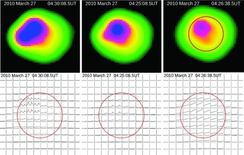
5.1.3 Direct imaging of emission from CME plasma

Though CMEs are routinely imaged in visible light using coronagraphs, and CME-driven shocks produce broadband radio emissions over several hundred MHz to as narrow as 20 kHz, the CME plasma itself has been difficult to observe directly. Metre and decimetre frequencies are regarded as the most suitable in which to try to image the synchrotron, gyrosynchrotron, and/or thermal bremsstrahlung emission from the CME plasma (Bastian & Gary Reference Bastian and Gary1997). Such measurements offer very useful and unique diagnostic capabilities, including the ability to constrain the CME magnetic field remotely. To date, however, only a few events have been confidently interpreted this way (e.g. Bastian et al. Reference Bastian, Pick, Kerdraon, Maia and Vourlidas2001; Maia et al. Reference Maia, Pick, Vourlidas and Howard2000). Observing these events is particularly challenging for existing instruments due to the large contrasts between the inherent brightness of the non-thermal emission from the CME plasma (weak) and solar disc (strong), and other phenomenon which are often simultaneously present (e.g. noise storms), and the large angular scales of this relatively weak emission. With its significantly higher dynamic range imaging ability and higher sensitivity to extended emission scales, owing to its numerous short baselines, the MWA should be the most suitable instrument yet for direct imaging of emissions from the CME plasma.

5.2.1 Faraday rotation

The observation of FR of background polarised radio sources (see also Section 3.3) is the only known remote sensing technique sensitive to the orientation and magnitude of the interplanetary magnetic field. Changes in FR associated with the passage of the solar corona or CMEs through the line of sight to spacecraft were convincingly detected using the telemetry signal from the Pioneer 6 and Helios satellites (Stelzried et al. Reference Stelzried, Levy, Sato, Rusch, Ohlson, Schatten and Wilcox1970; Bird Reference Bird1982; Bird et al. Reference Bird1985). More recently, coronal FR has been detected using VLA observations of radio galaxies as the Sun passes in front of them (Mancuso & Spangler Reference Mancuso and Spangler2000; Spangler & Whiting Reference Spangler and Whiting2009). The ability to routinely monitor and track CME magnetic fields would revolutionise the field of space weather.

FR measurements have been applied to many interesting studies of the nature of the solar corona and the solar wind, including to determine the mean magnetic field in the corona (Patzold et al. Reference Patzold, Bird, Volland, Levy, Seidel and Stelzried1987), to measure the power spectrum of coronal waves and turbulence as a function of distance (Efimov et al. Reference Efimov, Bird, Andreev and Samoznaev1996), to suggest the existence of intermittent waves at single locations (Chashei et al. Reference Chashei, Bird, Efimov, Andreev and Samoznaev1999), to support theoretical models of wave dissipation as a coronal heating mechanism (Hollweg et al. Reference Hollweg, Bird, Volland, Edenhofer, Stelzried and Seidel1982), and to study the structure of the heliospheric current sheet (Mancuso & Spangler Reference Mancuso and Spangler2000).

Studies so far have been severely limited by the paucity of suitable linearly polarised sources and the narrow fields of view of existing instrumentation (Spangler & Whiting Reference Spangler and Whiting2009). As discussed in Section 3.3, observations using the WSRT at 340–370 MHz have lead to detection of polarised extragalactic sources exhibiting typical polarised intensities of 20 mJy and readily measurable RMs (Wieringa et al. Reference Wieringa, de Bruyn, Jansen, Brouw and Katgert1993; Haverkorn, Katgert, & de Bruyn Reference Haverkorn, Katgert and de Bruyn2003a, Reference Haverkorn, Katgert and de Bruyn2003b, Reference Haverkorn, Katgert and de Bruyn2003c). In the few areas of the sky investigated in detail, these efforts reveal about one suitable polarised source every ~4 deg², as well as patches of diffuse polarised emission (Bernardi et al. Reference Bernardi2013), suggesting that there will be sufficiently numerous background sources to chart CMEs.

The combination of the sensitivity of the MWA, its low frequency of operation, and its wide field of view, along with the availability of a large number of polarised sources with sufficient flux density, present the possibility of being able to measure the coronal and heliospheric FR simultaneously to several different lines of sight and out to much larger distances from the Sun (~50 solar radii) than previously accessible. No measurements of FR due to CME plasma are available yet at large solar offsets; hence, we rely on simulations to build quantitative expectations. Jensen et al. (Reference Jensen, Hick, Bisi, Jackson, Clover and Mulligan2010) estimate the RM from CMEs to be ~0.05 rad m⁻² (12° at 150 MHz) at about 0.4 AU. Liu et al. (Reference Liu, Manchester, Kasper, Richardson and Belcher2007) also arrive at a similar estimate and also show that the FR time series from instruments like the MWA during the CME passage may be used to infer the helicity and size of the CME.

For multiple reasons, these are rather challenging measurements to make (Oberoi & Lonsdale Reference Oberoi and Lonsdale2013). Ionospheric RM, is 1–10 rad m⁻², more than an order of magnitude larger than the expected heliospheric or CME RM signature. This implies that we will need to achieve ionospheric RM calibration accuracies of a few per cent over large fields of view in order to study heliospheric RM. The quiet solar flux density is 10⁴–10⁵ Jy; hence, detecting 20 mJy sources requires polarimetric imaging dynamic range of about 10⁶, in the vicinity of a strong and variable Sun.

5.2.2 Interplanetary scintillation

As radio waves from a distant compact radio source propagate through the turbulent and inhomogeneous solar wind plasma, the incident plane wavefronts pick up phase corrugations corresponding to density inhomogeneities. These phase corrugations develop into intensity fluctuations by the time the wavefronts arrive at the Earth-based telescope. Due to the motion of the solar wind, the interference pattern produced by these intensity fluctuations is swept past the telescope giving rise to observed scintillations.

The evolution and dynamics of solar wind in the inner heliosphere dominates space weather effects. However, there are few techniques available to study the solar wind in this vast region. Historically, interplanetary scintillation (IPS) was the first remote sensing technique used to investigate the solar wind in this region (Hewish, Scott, & Wills Reference Hewish, Scott and Wills1964). More recently, the routine availability of observations from heliospheric imagers (e.g. STEREO) that image very large parts of the heliosphere using white light scattered from the solar wind electrons, have emerged as very useful tools for investigations in the inner heliosphere. These techniques, along with local in situ sampling provided by most satellite-based instrumentation, complement each other well since they cover different spatial scales and have led to a more complete characterisation of the solar wind than would have been possible with either of the data sets (e.g. Jackson et al. Reference Jackson, Hick, Buffington, Bisi, Kojima and Tokumaru2007; Dorrian et al. Reference Dorrian, Breen, Brown, Davies, Fallows and Rouillard2008).

Several new instruments are coming online to study IPS. Apart from the MWA, the new facilities include the LOFAR (Bisi et al. Reference Bisi, Fallows, Jensen, Breen, Xiong and Jackson2011; Fallows et al. Reference Fallows, Asgekar, Bisi, Breen and ter-Veen2012) and the Mexico Array Telescope (Mejia-Ambriz et al. Reference Mejia-Ambriz, Villanueva-Hernandez, Gonzalez-Esparza, Aguilar-Rodriguez and Jeyakumar2010). In addition, the Ooty Radio Telescope in India (P. K. Manoharan, private communication, 2012) and Solar Wind Imaging Facility (SWIFT) in Japan (Tokumaru et al. Reference Tokumaru, Kojima, Fujiki, Maruyama, Maruyama, Ito and Iju2011) are both undergoing considerable upgrades which will substantially improve their scientific capabilities.

For the MWA, the primary IPS observable will be the power spectrum of observed intensity fluctuations, although we will also employ a less commonly used observable, the normalised co-spectrum obtained from simultaneous observations at frequencies differing by a factor of ~2 (Scott, Rickett, & Armstrong Reference Scott, Rickett and Armstrong1983; Zhang Reference Zhang2007). Under the assumption of weak scattering, the interplanetary medium can be regarded as a collection of thin screens placed along the line of sight, and the IPS observable can be modelled as a weighted sum of the contributions from each of the thin screens. The physical parameters to which IPS is sensitive are (1) the velocity of the solar wind; (2) the level of electron density fluctuations, δn _e; (3) the spectral index of the δn _e power spectrum; (4) the inner scale for the power law governing δn _e; and (5) the axial ratio of δn _e.

Using an inversion process, it is possible to extract the global three-dimensional distribution of IPM parameters (Jackson et al. Reference Jackson, Hick, Kojima and Yokobe1998; Kojima et al. Reference Kojima, Tokumaru, Watanabe, Yokobe, Asai, Jackson and Hick1998; Asai et al. Reference Asai, Kojima, Tokumaru, Yokobe, Jackson, Hick and Manoharan1998; Oberoi Reference Oberoi2000; Bisi et al. Reference Bisi, Jackson, Hick, Buffington, Odstrcil and Clover2008, Reference Bisi, Jackson, Breen, Dorrian, Fallows, Clover and Hick2010; Dorrian et al. Reference Dorrian2010; Xiong et al. Reference Xiong, Breen, Bisi, Owens, Fallows, Dorrian, Davies and Thomasson2011). The most important bottleneck currently constraining the fidelity and resolution of the inversion of IPS data, and hence its science output, are the sparseness (both in space and time) and the non-uniformity of the sampling of the heliosphere afforded by the present generation instrumentation (Oberoi & Benkevitch Reference Oberoi and Benkevitch2010). The MWA will represent a significant advance in addressing the bottleneck of limited heliospheric sampling when its voltage capture system is completed. The MWA will have a sensitivity of ~70 mJy (1 s and 30.72 MHz), comparable to that of the SWIFT transit facility currently under commissioning in Japan. The MWA will boost the number of independent IPS measurements by up to a factor of ~30 over what is possible with most present-day systems. The southern hemisphere location of the MWA also complements the heliospheric coverage provided by the existing facilities, all of which happen to be in the northern hemisphere. Combining these data with other MWA observations like solar imaging and FR observations, and the observations from other sources such as STEREO, SDO, and HINODE, will provide a very comprehensive data set for characterising the inner heliosphere, monitoring and tracking CME evolution from close to the Sun to our terrestrial neighbourhood. Furthermore, the software framework being developed for handling the MWA IPS data could provide a common data repository, interface, and analysis tools for IPS data from observatories across the world (Oberoi & Benkevitch Reference Oberoi and Benkevitch2010).

5.3.1 Travelling ionospheric disturbances

TIDs are manifestations of middle-scale ionospheric irregularities arising as response to acoustic gravity waves. TIDs are frequently observed at high and middle latitudes (Bristow, Greenwald, & Villain Reference Bristow, Greenwald and Villain1996; Nicolls & Heinselman Reference Nicolls and Heinselman2007; Oliver et al. Reference Oliver, Fukao, Yamamoto, Takami, Yamanaka, Yamamoto, Nakamura and Tsuda1994, Reference Oliver, Otsuka, Sato, Takami and Fukao1997; Djuth et al. Reference Djuth, Sulzer, Gonzáles, Mathews, Elder and Walterscheid2004), and their activity and amplitudes vary depending on latitude, longitude, local time, season, and solar cycle (e.g. Kotake et al. Reference Kotake, Otsuka, Tsugawa, Ogawa and Saito2006; Hernández-Pajares, Juan, & Sanz Reference Hernández-Pajares, Juan and Sanz2006). They can be generated by auroral sources at the high latitude thermosphere, the passage of the solar terminator (Galushko et al. Reference Galushko, Beley, Koloskov, Yampolski, Paznukhov, Reinisch, Foster and Erickson2003), and storms, hurricanes, and tornados in the troposphere. Detailed information about the sources, energetics, and scale sizes of energy coupling from the lower atmosphere to the upper atmosphere, along with resulting ionospheric effects, is critical to developing a deep understanding of overall upper atmospheric energy balance. Measurements of TIDs at the VLA have been made since the early 1990s (Jacobson & Erickson Reference Jacobson and Erickson1993; Jacobson et al. Reference Jacobson, Carlos, Massey and Wu1995) and recent observations have been reported by Helmboldt et al. (Reference Helmboldt, Lazio, Intema and Dymond2012) and Helmboldt, Lane, & Cotton (2012). The fine grid over which the MWA calibration solutions will provide differential TEC measurements will provide detailed measurements of the propagation of TIDs over the array and TEC gradients or irregularities.

5.3.2 Storm enhanced density

The MWA is well sited to contribute to coordinate international investigations of the SED phenomenon (Foster Reference Foster1993). This process is responsible for some of the largest space weather effects at mid-latitudes (Coster & Foster Reference Coster and Foster2007) since it produces severe, temporally dependent electron density gradients. These gradients will be obvious in the differential TEC measurements made by the MWA. The geographic/geomagnetic pole offset in the southern hemisphere is anticipated to influence the development of SED near the MWA (Coster et al. Reference Coster, Colerico, Foster, Rideout and Rich2007; Foster & Coster Reference Foster and Coster2007; Foster & Erickson Reference Foster and Erickson2013). SED associated gradients have a practical consequence, as they cause large errors in GPS range measurements, and significantly degrade the high-precision positioning information provided by GPS systems. The MWA's longitude (~116° E) is very close to the longitude being extensively instrumented in the Asian sector as part of the Chinese Meridian project (~113°), and the conjugate longitude of ~64° W is within the field of view of the US-sponsored chain of incoherent scatter radars, in particular Millstone Hill. The combination of simultaneous measurements from these distributed sensors thus provides a unique way to determine mesoscale response to geomagnetic disturbances in the coupled geospace system. In particular, it will be possible to investigate whether there is a seasonal and universal time dependence of geomagnetic storm response by comparing American and Asian/Australian sector response to solar wind and CME forcing. Such effects have been predicted theoretically (Foster & Erickson Reference Foster and Erickson2013) but have not yet been confirmed by observations.

5.3.3 Ionospheric scintillation

Ionospheric scintillation can be defined as the rapid fluctuation of radio-frequency signal phase and/or amplitude, generated as a signal passes through the ionosphere. MWA observations using voltage capture capabilities will be uniquely suited for the exploration of ionospheric irregularities and scintillation. The voltage capture system should provide the ability to create array beams in post-processing that use the entire bandwidth and collecting area of the MWA, and that can be pointed independently anywhere within the MWA field of view. Such a system will provide scintillation measurements at multiple positions across the visible ionospheric region.

MWA array-beam observations will be augmented by data from specially designed GPS receivers at and near the MWA site that can measure L-band scintillation statistics. GPS TEC data from these receivers, when combined with data from a large number of newly deployed GPS receivers on the Australian continent, will provide important contextual information about the regional distribution of TEC around the MWA site. Other satellite-based remote-sensing platforms, including COSMIC, DMSP, and JASON, will also be available during overflights to provide further information about background ionospheric plasma and electrodynamic conditions in the ionosphere. A similar approach has been followed previously in the Combined Radio Interferometry and COSMIC Experiment in Tomography (CRICKET) campaign utilising the VLA (Dymond et al. Reference Dymond2008; Coker et al. Reference Coker, Thonnard, Dymond, Lazio, Makela and Loughmiller2009). This mix of data types allows for ionospheric specification from the global scale down to the regional scale.