Introduction

Icebergs are fragments of inland ice masses, which break off from the edges of ice sheets, shelves or glacier tongues (Reference PatersonPaterson, 1994;Reference Young, Turner, Hyland and WilliamsYoung and others, 1998). There are a number of reasons for the interest in monitoring icebergs. Most obvious is the fact that they present a serious hazard to marine traffic. For Antarctica, iceberg calving is the largest term of freshwater flux from the ice sheet into the ocean, but corresponding quantitative estimates reveal large uncertainties (Reference Jacobs, Hellmer, Doake, Jenkins and FrolichJacobs and others, 1992;Reference PatersonPaterson, 1994;Reference Silva and BiggSilva and Bigg, 2005). One reason for this is that only huge icebergs (lengths above 10 nautical miles or 18.5 km) have been monitored systematically (Reference Silva, Bigg and NichollsSilva and others, 2006). When icebergs melt, they affect the local stability of the ocean layers (Reference JenkinsJenkins, 1999; Reference Silva, Bigg and NichollsSilva and others, 2006). When the input of fresh water in the upper layers increases, the water column is stabilized. A reduction of freshwater input enhances the deep convection and leads to sea-ice thinning (Reference Schodlok, Hellmer, Rohardt and FahrbachSchodlok and others, 2006). Tracking of icebergs is useful for studying the mean currents of the upper ocean layers since they have a much stronger influence on the drift of larger icebergs than surface winds. Since icebergs transport meteoric dust, their melting fertilizes of the upper ocean layers. Grounded icebergs influence the local benthic ecosystem (Reference Gutt and StarmansGutt and Starmans, 2001).

A number of different satellite sensors have been used for monitoring icebergs. The employment of data from optical sensors such as the Thematic Mapper (TM) on NASA’s Landsat or the Medium-Resolution Imaging Spectrometer (MERIS) on the European Space Agency (ESA)’s Envisat requires suitable cloud and light conditions. This restriction does not hold for imaging radars such as the synthetic aperture radar (SAR) on board European Remote-sensing Satellites 1 and 2 (ERS-1/-2) or the Advanced SAR (ASAR) on board Envisat. With their high spatial resolution of 30 m the detection of even small icebergs with an edge length of about 100 m is possible.

In this study, we deal with the unsupervised identification of icebergs in SAR images. Automatic detection of icebergs using SAR images has been investigated in a number of studies. The simplest method for object detection is to define intensity thresholds for separating different object classes (e.g. icebergs, sea ice and water). This approach was used for example by Reference Willis, Macklin, Partington, Teleki, Rees and WilliamsWillis and others (1996). They focused on the detection of icebergs in ERS-1 images, mainly under open-sea conditions. In order to eliminate smaller targets (clusters less than five pixels) with intensities similar to that of icebergs, they applied morphological filters. Reference Williams, Rees and YoungWilliams and others (1999) developed a method for identification of icebergs based on edge detection and segmentation by pixel bonding. Their argument for such an approach is that it is important to identify icebergs as individuals even if they are located very close to each other (such as in iceberg clusters). They carried out tests on ERS-1 images and found that the technique was not reliable for icebergs less than six image pixels in size, that it generally overestimated the iceberg area and that it was sometimes difficult to separate segments belonging to the iceberg class from sea-ice or open-water segments. Taking the shortcomings into account, this approach was also used by Reference Young, Turner, Hyland and WilliamsYoung and others (1998) for a detailed study of spatial distribution and size statistics of icebergs in the East Antarctic sector. In the method presented by Reference Silva and BiggSilva and Bigg (2005), edges between segments of different backscattering coefficients are determined in windows of different sizes, i.e. on different spatial scales. The results of different scales are combined in order to obtain precise edge positioning with robustness to noise. In subsequent steps, algorithms are applied for merging segments belonging to the same object and to identify icebergs by applying a set of criteria that define typical ranges of the backscattering coefficient and of geometrical parameters based on area, perimeter and major/minor axis.

The application of the methods described above relies on a detailed knowledge of radar intensity variations in the marine polar environment. To our knowledge, a comparative study of backscattering characteristics of icebergs and the ‘background’, i.e. sea ice or open water or a mixture of both around the icebergs, is still lacking for the Antarctic. With our study we intend to fill this gap. The sensitivity of the backscattering intensities of open-water surfaces to wind speed and direction is a well-known phenomenon (e.g. Reference Power, Youden, Lane, Randell and FlettPower and others, 2001). For a number of reasons, icebergs must also be identified when captured in sea ice during winter. Larger areas of the western Weddell Sea are covered by perennial ice. For this ice type, Reference HaasHaas (2001) found a significant seasonal cycle of the backscattered radar intensity. Sea-ice structures, such as deformation zones or large cracks on the km scale, are characterized by a high backscattering intensity similar to icebergs.

The main objectives of this paper are to analyze variations of backscattering signatures from icebergs, sea ice and open- water surfaces and their dependence on environmental conditions. Considering the results, a methodology is developed for automated detection of icebergs, focusing in particular on icebergs with a longitudinal axis significantly smaller than 10 nautical miles (18.54km). The paper is structured as follows. We give a short overview regarding iceberg and sea-ice physical properties and introduce the model we used for the statistical distribution of radar intensities. After information is provided on the available SAR images and the areas of investigation, the observed backscattering intensities and intensity statistics of icebergs and background (sea ice, water surface) are presented. From the statistics a detection method is derived and applied to a number of SAR images. A performance study using a reference dataset of manually identified icebergs provides quantitative measures for an assessment of the unsupervised method and possible seasonal differences. Also included are examples for estimating the total iceberg area for a given region by employing the developed automated method in comparison to reference data, which also demonstrate problems that occur in the unsupervised iceberg detection.

Icebergs and Sea Ice In SAR Images

Icebergs are categorized in a number of different size classes: (a) growler (0-5 m), (b) bergy bit (5-15 m), (c) small berg (15-60 m), (d) medium berg (60-120 m), (e) large berg (120-220 m) and (f) very large berg (>220 m). The shape categories are: (1) tabular, (2) non-tabular, (3) domed, (4) wedge, (5) dry dock, (6) pinnacle and (7) blocky (Reference Jackson and ApelJackson and Apel, 2005, p.411). In satellite images, the different shape categories can rarely be distinguished.

The radar backscattering coefficient of an iceberg is the sum of surface and volume contributions. For the analysis of radar signatures, the variable surface characteristics of icebergs have to be considered. The upper part of many icebergs is covered by snow or firn. Smaller icebergs may have rolled over. In such cases, their surface consists of pure ice, which may quickly become weathered. The scattering intensity depends on the iceberg’s shape and the roughness of its surface and on the fraction, size and shape of cracks, air bubbles and impurities in the ice volume (Reference Willis, Macklin, Partington, Teleki, Rees and WilliamsWillis and others, 1996;Reference Young, Turner, Hyland and WilliamsYoung and others, 1998). The penetration depths of the radar signal at C-band range from 3 to 14 m depending on the dielectric properties and the volume structure (e.g. presence of air inclusions;Reference Power, Youden, Lane, Randell and FlettPower and others, 2001). In L-band SAR images, bright ghost signals were found close to icebergs (125-600 m in size) which were explained by time-delayed reflections of radar waves from the ice-water interface at the bottom of an iceberg (Reference Gray and ArsenaultGray and Arsenault, 1991). Under surface freezing conditions, icebergs appear as bright objects against a darker background of sea ice or open water at low to moderate wind speeds. In regions where the summer air temperatures are at or above the melting point, liquid water and/or wet snow on the iceberg surface reduce the volumescattering contribution significantly. In this case, the icebergs stand out as dark targets.

Sea ice is a mixture of freshwater ice, liquid brine, solid salt crystals and air voids. Its radar backscattering characteristics depend on the ice salinity and temperature, fraction, size and shape of air bubbles and brine inclusions, small- scale surface roughness (with undulations on the order of the radar wavelength) and large-scale (m to km) surface structure. Older ice is less saline. Hence, radar waves penetrate deeper into the ice and the volume-scattering contribution increases. Various processes at the ice surface or the snow-ice interface, such as melt-freeze cycles, flooding or the formation of superimposed ice, affect the total backscattering magnitude and the balance between surface and volume scattering.

For the definition of intensity thresholds between icebergs and their background, the statistics of the radar back- scattering coefficients need to be considered. Even if the ‘true’ backscattering coefficient is constant over a larger area comprising several pixels in a SAR image, the measured values reveal variations due to speckle (e.g. Reference Oliver and QueganOliver and Quegan, 1998). Speckle appears as a grainy texture in radar images, which is caused by random constructive and destructive interferences of the scattered signals that occur within each SAR resolution cell. The magnitude of variation caused by speckle is estimated from the effective number of looks (here denoted as L), which is a function of mean square and variance of the radar intensity (Eqn (2) below). For this purpose, we used a window of 50 × 50 pixels for the calculation of mean and variance. Intensity variations due to speckle can be modeled by a gamma distribution (Reference Oliver and QueganOliver and Quegan, 1998). We tested this for icebergs, sea ice and open water and found only a moderate correspondence between observed and modeled distributions. Therefore we suppose that the ‘true’ radar backscattering coefficient varies on spatial scales that are smaller than the window dimension that we used for calculating mean and variance. In this case the K-distribution can be applied to describe the radar intensity statistics. The K-distribution is based on the assumption that the ‘true’ backscattering coefficient is gamma-distributed and that speckle and radar intensity show variations on different scales so that they can be treated separately (Reference Oliver and QueganOliver and Quegan, 1998). Variations of radar intensities over an iceberg may be caused, for example, by a changing local surface slope (considering the different shapes of icebergs) or local variations of properties influencing the scattering. The K-distribution is given by:

(1)

where L is the effective number of looks, v is the order parameter, μ is the mean backscattering intensity, Γ(*) is the gamma function and K_v-L (*) is the modified Bessel function of the second kind, of order v-L. The effective number of looks is obtained from:

(2)

where var is the variance of the backscattering intensity within the area of the window used for calculating L (Reference Oliver and QueganOliver and Quegan, 1998). The order parameter v can be derived from an adapted formula of the moment analysis (Reference ReddingRedding, 1999):

(3)

Data, Areas of Investigation and Image Collection

For our study we used Envisat ASAR and ERS-2 data, the former in Image Mode (IM) and Wide Swath Mode (WS). The IM and ERS-2 images are provided at a pixel size of 12.5m × 12.5m with an effective spatial resolution of 30 m × 30 m and a local incidence angle between 19.2° and 26.7° (IM image swath IS2) and 19.5° and 26.5° (ERS-2), respectively. The corresponding values for WS images are 75 m × 75 m for the pixel size, with an effective spatial resolution of 150 m × 150 m and local incidence angles between 17° and 43°. All ASAR images were recorded at C- band (5.3 GHz) at HH polarization, while the ERS-2 data are VV-polarized. Reference Sandven, Babiker and KlosterSandven and others (2007) found that HH polarization showed the most reliable results for iceberg identification. The SAR images were georeferenced and calibrated. We reduced the image size by averaging two adjacent pixels, hence doubling the pixel size, but reducing speckle. Since we focus on ocean regions, the calibration of the SAR images did not include terrain correction.

Two regions in the Weddell Sea were chosen for investigations. The criterion for selection was to cover different environmental conditions such as freezing and melting, sea-ice concentrations between 0% and 100% and different sea-ice types. Changing conditions affect the absolute radar intensities as well as the relative intensity contrast between the icebergs and the surrounding sea-ice or water surface.

The first region is located in the southern Weddell Sea, north of Berkner Island (Fig. 1). It is covered with perennial sea ice (http://nsidc.org/data/nsidc-0192.html), and air temperatures are at or above the melting point for only a few days during the year (see http://www.ecmwf.int/ and Fig. 4 below). To investigate a complete seasonal cycle, 61 Envisat IM images available for the region of interest (ROI) and spread in time across the year 2006 were used. These data were complemented by 11 Envisat WS images, one at the beginning of each month starting in February 2006 (Fig. 1).

Fig. 1.

Overview of the Weddell Sea region, indicating the two study regions and the positions of the images. The coast and grounding lines as well as the island contours are taken from http://nsidc.org/data/nsidc-0280.html.

The second test site is a region at the tip of the Antarctic Peninsula (Fig. 1), which is subject to significant changes in environmental conditions over the year. During the summer months, air temperatures are mostly above freezing point and the sea-ice concentration is close to zero. In the winter months, when the air temperatures are below zero, the sea- ice cover is often closed (10/10 concentration). For this test site we have received 15 ERS-2 images recorded between 16 October 2000 and 18 January 2003 (Fig. 1). The temperature information for the observation period was taken from the European Centre for Medium-Range Weather Forecasts (ECMWF) database.

Backscattering Statistics

For the statistical analyses of the ASAR IM image sequence, 566 ROIs were defined on icebergs, whereby each ROI covered the whole visible area of the respective iceberg. Hence, the area of each iceberg could be calculated from the size of the ROIs using standard modules of the image-processing software. On sea ice, 600 rectangular ROIs were defined. The number of pixels covered by the area of each ROI was variable in the case of the icebergs, but was fixed to 400 × 400 pixels for sea ice and open water. In each of the ASAR and ERS-2 scenes, ten icebergs and just as many sea-ice/open-water ROIs were defined. The largest icebergs of up to 90 km² are covered in their entirety only in the WS images;in the IM images, only parts of them are visible. The smallest icebergs that could be identified clearly in WS were about 0.2 km² in area;in IM the minimum area was 0.02 km². The positions of the respective ROIs in the images were chosen randomly. In new or first-year sea-ice regimes, icebergs can be clearly identified because their backscattering coefficient is higher by about 5dB up to 10 dB (Reference Young, Turner, Hyland and WilliamsYoung and others, 1998). In wind-roughened open- water or deformed sea-ice regimes, the iceberg back- scattering coefficients do not differ significantly from their surrounding. The visual detection of icebergs in radar images is nonetheless possible because of the radar shadow at the side of an iceberg averted from the incoming radar waves and because the radar signature of icebergs is usually more homogeneous than that of sea ice or wind-roughened open water. We did not avoid multiple counts of individual icebergs in the image sequence since we could not exclude temporal variations of the radar signatures. In the area of test site 1, temporal variations of the backscattering coefficients of single icebergs and the differences between the back- scattering coefficients of different icebergs were considerable over the year 2006. However, we did not recognize systematic changes as a function of season.

Table 1.

The average, maximum and minimum variance-to- squared-mean ratio (VMR) of the ROIs used to calculate the backscattering coefficients shown in Figure 3

Southern Weddell Sea region

We started the investigation by concentrating on the seasonal variation of iceberg and sea-ice backscattering intensities in the southern Weddell Sea region, taking into account the effect of the radar incidence angle and the orientation of the iceberg relative to the radar look direction. Five icebergs of different areas (4-11 km²) and shapes were selected, which could be identified in most images of the image sequence. The results are shown in Figure 2. The mean backscattering intensities of the five icebergs vary as a function of time and differ between the image modes (IM and WS). To investigate the relative contribution of different factors influencing the backscattering coefficients, a multiple correlation coefficient (r _a.bcd ) with one goal parameter (mean backscattering intensity a) and three independent impact parameters (incidence angle b, orientation c and recording day d) was calculated. This resulted in r _a.bcd = 0.11, which means that none of the impact parameters had much influence on the backscatter coefficients. Relatively, the incidence angle had the largest impact with r _a.b = -0.26. The negative value indicates that the backscattering coefficient decreases with increasing incidence angle. The orientation and recording day show almost no correlation with the backscattering coefficient (r _a.c = -0.1 and r _a.d = 0.12). All correlation coefficients were calculated at a significance level of 99%. We note that in single cases, the backscattered radar intensity of an iceberg may vary between SAR images acquired at different look directions, dependent on the orientation of reflecting facets on the iceberg surface (Reference Sandven, Babiker and KlosterSandven and others, 2007). These facets are of sizes on length scales of a few radar wavelengths. From position changes of the five icebergs in the SAR image sequence we obtained a value for the iceberg drift of approximately ≤16 km a^-1. Looking at SAR images of this region recorded at the end of 2010, all icebergs can still be found. Since they are located over Berkner Bank, one possible reason for this very slow drift (and observed iceberg rotations) could be that they may be in occasional contact with the sea floor.

Fig. 2.

Mean backscattering coefficient of five icebergs as a function of the day of the year 2006. Black circles are values obtained from IM images; black triangles indicate values from WS images. Gray rectangles represent the orientation of the longitudinal axis of the iceberg relative to the illumination direction. Numbers are the mean radar incidence angle. The vertical lines separate seasons, with the first and last sections being Antarctic summer. Icebergs 3 and 4 are located close to each other; icebergs 1, 2 and 5 are separated from icebergs 3 and 4 and from each other by larger distances.

The sea-ice backscattering coefficient changes, in particular over the transition from freezing to melting conditions and vice versa. According to Reference HaasHaas (2001), Antarctic sea-ice backscattering reveals a seasonal cycle. The radar back- scattering coefficients are largest in late summer. Back- scattering changes are caused by the metamorphosis of snow, the formation of ice layers in the snow and superimposed ice. These processes result in coarser snow grain sizes and an increasing number of air bubbles in the near-surface layer, which increases the radar backscattering coefficients (Reference HaasHaas, 2001). Under such conditions, the intensity contrast between icebergs and sea ice would be smallest in summer.

In order to consider a potential sensitivity of the intensity contrast to the season, we divided our data accordingly. The numbers of available IM images (WS images) are 6 (3) for spring, 14 (2) for summer, 20 (3) for autumn and 21 (3) for winter. The number of identified icebergs varies between 62 in spring and 201 in winter. Huge icebergs (>10 nautical miles (18.54 km), named and monitored by the US National Ice Center) were excluded from this analysis.

Figure 3 shows that the observed ranges of the back- scattering coefficient at a given incidence angle are large both for icebergs and sea ice. We attribute this to local changes of iceberg properties on the surface and in the subsurface layer affecting the scattering processes. In the WS images, only a few icebergs were observed at lower incidence angles. According to Figure 3, the average incidence angle sensitivity does not differ significantly for icebergs and sea ice. In general, the sensitivity is smallest for volume scattering, slightly larger for very rough surfaces and largest for smooth surfaces (e.g. Reference FungFung, 1994, ch. 2). Figure 3 indicates that on average the contribution of volume scattering or scattering from very rough surfaces is dominant for icebergs and sea ice. The range of sea-ice backscattering coefficients in Figure 3 (obtained for HH polarization) compares well with the results of ground-based scatter-ometer measurements over rough first-year ice and over second-year ice reported by Reference Drinkwater, Hosseinmostafa and GogineniDrinkwater and others (1995). Their measurements were carried out at VV polarization. For rougher surfaces and in the case of volume scattering, the difference between VV and HH polarization is small.

Fig. 3.

Mean values of (a) iceberg and (b) sea-ice backscattering coefficients as a function of the incidence angle and season. The solid line shows the mean trend. For each graph the correlation coefficient and the slope of the linear regression are given in the top right corner.

In Table 1, the average, maximum and minimum variance-to-squared-mean ratios (VMRs) are presented. For the statistical analysis, we estimated the number of looks for the pre-processed images by calculating mean and variance for a number of apparently texture-free areas (Eqn (2)). The corresponding VMRs are on average 0.16 for IM data and 0.039 for WS. This agrees well with the minimum average values of the VMR listed in the table. Values close to the minimum indicate that the radar intensity variation is caused only by speckle. Since the maximum and mean VMRs in Table 1 are significantly larger than the minimum values, we also have to consider ‘real’ variations of the backscattering coefficient itself (as opposed to ‘apparent’ variations due to speckle) over areas which are similar in size to the ROIs used for evaluating the VMR. Hence, the choice of the K- distribution for describing the variations of the measured backscattering coefficient is justified. Maximum and mean VMRs are considerably larger for icebergs than for sea ice, which is interpreted as a larger variability of the ‘true’ backscattering coefficient on icebergs.

According to Figure 3, the backscatter intensity from icebergs is on average about 7-8 dB larger than from sea ice, independent of incidence angles and season. This is in contradiction to Reference HaasHaas (2001), who found a spatially partly rapid rise of the backscattering coefficient for sea ice measured by the ERS-1/-2 scatterometer in West Antarctic waters (Weddell, Amundsen and Bellingshausen Seas) during summer months. This was attributed to layers of superimposed ice. This type of ice forms at air temperatures close to or above 0°C due to melting and refreezing processes at the snow-ice interface and contains many air bubbles, which scatter the radar waves at C-band. In such a case, the intensity contrast between icebergs and sea ice is lowest in summer, provided that radar backscattering coefficients of icebergs do not vary over the season (we have no evidence for this in our data). Specifically for the southern Weddell Sea, at our test site location, patterns of seasonal variations of the sea-ice backscattering coefficients with distinct summer maxima were only observed for single years (Reference HaasHaas, 2001, Fig. 2).

The meteorological data for summers 2005/06 and 2006/ 07 show temperatures alternating between values above and below 0°C (Fig. 4), which means that superimposed ice could have formed. Therefore we have no direct evidence that the existence of superimposed ice is less widespread at our test site than in other areas investigated by Reference HaasHaas (2001). The conclusion is that our results presented in Figure 3, which do not reveal any significant variations of the intensity contrast between icebergs and sea ice, may not be valid in general.

Fig. 4.

Air temperature for the years 2005, 2006 and 2007 for the test site north of Berkner Island. Daily temperature taken from ECMWF. The error bars represent the standard deviation of the monthly mean.

In order to investigate whether there are systematic regional variations in backscattered radar intensities of icebergs, the mean backscattering coefficients in the 2025° incidence angle interval are presented for autumn in Figure 5. The backscattering coefficient varies by about 7 dB in a relatively small region, but a clear large-scale pattern of variation cannot be discerned.

Fig. 5.

Mean backscattering coefficients of icebergs in IM (dots), shown for autumn observation over the southern Weddell Sea test site for the 20–258 incidence angle interval.

We selected different icebergs for the analysis of local backscattering variations and assumed that they broke off at different locations along the coast of Antarctica. This means that one has to consider local/regional differences of ice properties at the calving sites and the time that each iceberg drifted from its calving site to the positions shown in Figure 5. Older icebergs have been affected by one or more summer melting periods. Hence it can be expected that the surface and subsurface characteristics and therefore the backscattering characteristics of the icebergs differ.

For the development of classification rules, we investigated how well the measured backscattering coefficients of icebergs and sea ice are matched by the K-distribution. Although we found a relatively weak sensitivity of the backscattering coefficient to the incidence angle both for icebergs and rough sea ice, we calculated histograms for each season as a function of incidence angle, considering the fact that in other regions around Antarctica smooth first- year ice is more common. An example is given in Figure 6. Here the histograms were generated from the pixel values of all icebergs that were visually identified in the SAR images acquired during winter. Attention was given to obtaining a representative selection of icebergs (different sizes with their positions spread all over the images). The quality of the theoretical K-distributions was tested with the Kolmogorov- Smirnov goodness-of-fit test, which uses the maximum absolute value of the deviation between the measured and the theoretical cumulative distributions (P), in our case for the backscattering coefficients in linear scale. The corresponding P-values were 0.02-0.21, with means of 0.08 for icebergs in IM images, 0.06 for sea ice in IM images, 0.11 for icebergs in WS images and 0.09 for sea ice in WS images. All measured distributions could be modeled successfully by the K-distribution at a high significance level (99%). This was checked using the quality value P which should be <0.23 for our sample size (N = 50), if theoretical and measured distributions were compared on the 99% significance level.

Fig. 6.

Example of histograms of the measured backscattering coefficients of (a) icebergs and (b) sea ice in the southern Weddell Sea during winter. Backscattering coefficients are given in linear scale. The thick black line shows the K-distribution calculated using Eqn (1). For each graph the incidence angle interval is provided in the upper left corner and the P -value of the Kolmogorov-Smirnov test in the upper right corner.

Antarctic Peninsula region

The ERS-2 images from the tip of the Antarctic Peninsula were pre-processed in the same way as the Envisat images for the southern Weddell Sea test site. The images we had available are from spring and summer of 2000-2003. Periods for which the ocean surface is ice-free or ice concentration is low occur frequently during summer months at this test site. Rapid changes of the ‘background’ radar intensity are typical for such periods due to changing wind and wave conditions. The data were separated into a group of images with icebergs that appeared bright and another group with dark icebergs. Dark icebergs were found only in the warmer summer months (December, January, February). In spring, only bright icebergs were observed, and two summer images, recorded on 17 February 2001, also showed bright icebergs.

The sea-ice concentration was nearly zero in the warmer summer months. Therefore we included an investigation of the backscattering coefficients of the open-water areas. The available images, which contain black icebergs, were recorded on four dates: 15 January, 18 January and 14 December 2002 and 18 January 2003. Wind conditions, which were taken from the ECMWF, were highly variable in the ROI (Table 2). The well-known sensitivity of ocean backscattering coefficients to wind speed and direction is clearly demonstrated in Table 2. The average backscattered intensities of the icebergs do not change significantly.

For further investigations, we used the images recorded in December 2002 and January 2003 because they cover a relatively large number of ‘dark’ icebergs. The histograms in Figure 7 are two examples of the measured backscatter coefficient distributions for dark icebergs and open water in comparison with the K-distribution. For all cases there is a decrease in the occurrence of larger backscattering intensities at higher incidence angle intervals, as expected. The relatively large differences between the open-water histograms from December and January are caused by the different wind conditions (Table 2). For this test site, we obtained maximum deviations between the measured and the theoretical distributions (P) from 0.04 to 0.17, with means of 0.06 for bright icebergs, 0.07 for dark icebergs, 0.07 for sea ice and 0.09 for open-water regions. The Kolmogorov-Smirnov goodness-of-fit tests resulted in good agreement between the measured and theoretical distributions at a high significance level (99%).

Fig. 7.

Histograms of the measured distributions of backscattering coefficients for (a) dark icebergs and (b) open water on 14 December 2002 and (c) dark icebergs and (d) open water on 18 January 2003. Backscattering coefficients are given in linear scale. The thick black line shows the theoretical K-distribution. For each graph the incidence angle interval is provided in the upper left corner and the quality value P of the Kolmogorov–Smirnov test in the upper right corner. On 18 January 2003, there are no open-water ROIs available within the incidence angle range 15–20º.

Table 2.

Wind conditions, air temperature, mean backscattering coefficients (σ⁰) of open water and icebergs (dB) and satellite flight direction, on different days. The platform heading is given corresponding to the scene center in degrees from north

Detection of Icebergs

In this section, we describe the development of a threshold- based detection method for icebergs, i.e. the partitioning of the backscatter values into classes of icebergs, sea ice and open water. Our method is based on a pixel-by-pixel approach. For the investigations presented in the preceding sections we separated the data by season, and for each season we arranged the data by different incidence angle intervals of 5° or 10° width, dependent on the number of iceberg pixels. To these groups of data, theoretical K- distribution functions were fitted (e.g. Figs 6 and 7). We used the respective theoretical functions to derive relative cumulation distributions from which intensity thresholds between icebergs and sea ice or open water were determined (Fig. 8), considering different conditions such as bright icebergs surrounded by sea ice or dark icebergs surrounded by open water. For bright icebergs (in the southern Weddell Sea region and spring at the Antarctic Peninsula) and for the ocean surface at higher wind speeds (summer at the Antarctic Peninsula), the K-distributions were cumulated from the large to the small backscattering coefficients, and for dark icebergs (summer at the Antarctic Peninsula) and sea ice (in the southern Weddell Sea region) from small to large backscattering coefficients. The threshold was chosen at a relative cumulative frequency of 0.95 (horizontal line in Fig. 8). We emphasize that the result obtained for the Antarctic Peninsula is only valid for the specific wind conditions on 18 January 2003, but it is a useful example for demonstrating the principle. It is clear, however, that detection of dark icebergs is most reliable for high wind speeds and detection of bright icebergs for low wind speeds.

Fig. 8.

(a,b) Cumulative K-distributions of icebergs (bold black solid lines) and sea ice (black dashed lines) derived from (a) IM images acquired in the southern Weddell Sea (SWS) in spring at an incidence angle of 25–30º and (b) WS images acquired in the SWS in summer at an incidence angle of 35–45º. (c) Cumulative Kdistributions of the ocean surface (black dashed line) and dark icebergs (bold solid black line) at incidence angles of 15–20º at the Antarctic Peninsula (AP). Backscattering coefficients are given in linear scale. Horizontal lines mark a cumulative relative frequency of 0.95; vertical lines correspond to thresholds for the backscattering coefficients of icebergs, sea ice and open water. Gray areas represent the backscattering range classified as ‘mixture’; diagonal hatched areas indicate the class ‘sea ice/open water’ and white areas cover the class ‘icebergs’.

The range of backscattering coefficients shown in Figure 8 was separated into three classes: (1) icebergs (white area), (2) mixture (gray area) and (3) sea ice (diagonal hatched area). In general, the positions of the 0.95 relative frequency threshold are different for icebergs and sea ice/open water. The differences between the 0.95 thresholds for icebergs and for sea ice are shown for all incidence angle intervals over a whole seasonal cycle for the Weddell Sea test site in Figure 9, using IM and WS data. Positive values are optimal for detection. They indicate that the number of iceberg and sea-ice pixels with identical values of the backscattering coefficient is small (Fig. 8b and c). Negative differences mean that the 0.95 cumulative frequency level of the icebergs is reached at lower backscattering coefficients than for sea ice (Fig. 8a). Since the final iceberg threshold is determined by the upper intensity limit of the mixture zone (in case of bright icebergs), it corresponds to a cumulative frequency level less than 0.95. This means that more sea-ice pixels and fewer iceberg pixels are classified correctly. The results presented in Figure 9 reveal a weak advantage for iceberg detection when spring and summer data are used. We assume that the larger negative threshold differences found in the autumn and winter IM images are related to ‘unfavorable’ sea-ice conditions characterized by patterns of relatively high backscattering intensities due to sea-ice deformation. Overlaps between the classes ‘icebergs’ and ‘sea ice’ were in general smaller in the WS images than in IM data. This may be due to a ‘smearing’ effect on the backscattering signature of narrow sea-ice deformation patterns within one pixel of the coarse-resolution image. The threshold difference is in general dependent on the intensity contrast between icebergs and sea ice and hence on local and temporal variations of sea-ice conditions.

Fig. 9.

Mean difference of 0.95 thresholds (at linear scale) between icebergs and sea ice for each season at the southern Weddell Sea test site. Circles represent IM images, and triangles represent WS images. The gray shades indicate the incidence angle range.

As a next step, the derived thresholds were applied to all images available for our study, on a pixel-by-pixel basis, considering the respective incidence angle range. Each pixel was then marked by a number indicating the class. Figure 10a shows the zoom-in of an unfiltered SAR image covering one large iceberg surrounded by sea ice of different age and a lead, which was either a calm open-water surface or thin new ice (black in Fig. 10a and e). The different gray tones in Figure 10a correspond to radar intensities given as σ⁰ in linear scale. The result after applying the detection thresholds is depicted in Figure 10b. The iceberg is identified very well, but there are also false detections (sea-ice deformation features identified as icebergs) and missing pixels within the iceberg. As shown by Reference Willis, Macklin, Partington, Teleki, Rees and WilliamsWillis and others (1996), morphological filters may help to reduce the false detection rates. For detailed information on morphological filters the reader is referred to Reference Haralick, Sternberg and ZhuangHaralick and others (1987). An opening filter, which is composed of morphological erosion followed by morphological dilation, at a kernel size of 3 × 3 pixels was applied to the threshold image. The result is not satisfying (Fig. 10c). To fill gaps between single iceberg targets, a closing filter (dilation followed by erosion), at a kernel size of 3 × 3 pixels, was used in a next step. The number of missing pixels over the iceberg was reduced, but the remaining gaps are still numerous (Fig. 10d). Considerably improved detection was achieved by using an enhanced Lee filter (kernel size 3 × 3 pixels, applied to the starting image, Fig. 10e) before classification by thresholds (Fig. 10f). The enhanced Lee filter reduced the image speckle while preserving the texture (Reference Lopes, Touzi and NezryLopes and others, 1990). Figure 10g and h show the results of morphological filtering.

Fig. 10.

Subset of an IM image in the southern Weddell Sea region from 1 November 2006. (a) Input (linear σ ⁰); (b) classification by thresholds; (c) application of opening filter; (d) application of an additional closing filter; (e) image after enhanced Lee filtering of the input data (a); and (f–h) same processing steps as (b–d). Image credits: ESA. The iceberg has a longitudinal axis of 18 km.

The performance of the different processing steps was tested by comparing the results of the threshold-classified and filtered images with the manually chosen icebergs, sea ice and open-water ROIs as reference. The result of this comparison for the different seasons at the Weddell Sea test site is shown in Figure 11. The height of the bars shown in Figure 11 gives the percentage of the correctly classified iceberg and sea-ice pixels. This means, for example, that in IM (WS) images, on average 2.6% (5.9%) of the iceberg pixels are erroneously classified as sea ice during summer and 8.7% (6.7%) during winter, using the M5 processing chain. In the case of sea ice, the corresponding fractions of pixels classified as iceberg are 1.1% (16.7%) for summer and 2.9% (2.5%) for winter data. When morphological filters are applied, wrongly classified areas of small size are already removed. The sea-ice classification is clearly more accurate in the IM images than in the WS data. This agrees with the result presented in Figure 9. There, negative threshold differences indicate that the thresholds are shifted towards higher intensity values than those corresponding to the 0.95 cumulative frequency level of the icebergs. However, for the result presented in Figure 11 the spatial distribution of the pixel is important in the cases where filters are applied, so only the M1 case can be compared directly with Figure 9.

Fig. 11.

Performance of the different processing steps shown in Figure 10 for the southern Weddell Sea (SWS) test site. Bars are as follows: M1= threshold; M2= threshold and opening filter; M3= threshold, opening and closing filter; M4= enhanced Lee filter and threshold; and M5= enhanced Lee filter, threshold, opening and closing filter. Sp: spring; Su: summer; Au: autumn; Wi: winter.

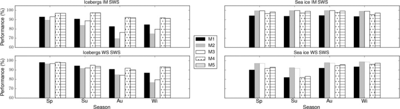
In the case of icebergs, the application of the opening filter on the threshold images, without first applying the enhanced Lee filter for speckle reduction, deteriorates the detection performance (M1 versus M2 bars, Fig. 11). The successive use of the closing filter improves the result (M3 bars, Fig. 11). If an enhanced Lee filter is employed before classification, the detection accuracy increases (M1 versus M4 bars, Fig. 11). However, morphological filtering does not improve the result (M4 versus M5 bars, Fig. 11). In the case of sea ice, the application of morphological filters on the threshold images, without a preceding enhanced Lee filter, was beneficial (M2 and M3 bars, Fig. 11). The enhanced Lee filter increased the classification accuracy only slightly (M4 versus M1 bars, Fig. 11) and the gain of the morphological filters was only marginal (M5 versus M4 bars, Fig. 11). The results indicate that in general it is sufficient to apply the enhanced Lee filter followed by a threshold operation to separate icebergs and sea ice. The only exception was found for sea ice in WS images, for which the morphological filtering applied on M1 images leads to considerable improvement in classification accuracy, in particular for spring and summer data. For IM images, spring and summer reveal slightly better classification results. For the WS data, we have no clear evidence for a particular season being optimal for iceberg detection. In summary we found that the application of different filters on the input SAR image influences the classification result, in some cases considerably. However, we could not establish a generally valid optimal filtering approach, which comprises IM and WS images and different sea-ice conditions and, in the case of open water, different wind conditions.

Test Cases: Estimation of Total Iceberg Area

We tested the practical application of the detection algorithm in sea-ice-covered regions and applied it to the problem of estimating the total iceberg area. Two IM images recorded on 4 November 2006 in the southern Weddell Sea were combined in a mosaic and subsequently used for iceberg detection. For a direct comparison, ROIs were manually defined, each following the contour of one of the 29 icebergs clearly visible in the mosaic. The iceberg areas, calculated from the sum of the pixels in the ROI (pixel size = 25 m × 25 m = 625 m²), varied between 0.02 and 728.75 km². We use these values as reference in the comparison with the results of the automatic iceberg classification and iceberg sizes derived from it. Since we selected icebergs that could be visually identified without any problems in the SAR mosaic and covered at minimum >30 pixels, we regard our reference areas as highly reliable. Potential errors in the visual inspection can only occur along the edges of the ROI when pixels reveal backscattering values that cannot be clearly associated with one class (iceberg, sea ice, open water). In the visual inspection, this problem does not occur for such pixels inside the ROI.

The automatic (or unsupervised) determination of iceberg sizes is carried out on the basis of the classified images. We applied the M5 processing chain to the image mosaic (i.e. enhanced Lee filter, threshold, opening and closing filter) and the intensity thresholds for spring. The resulting image is then the input to a pixel-oriented segmentation algorithm which is a standard module of the image-processing software used. Here segments, i.e. clusters of connected pixels, are identified and marked so that the individual segments can be separated automatically afterwards. In relation to our visual inspection of the images, we selected 30 pixels as the minimum cluster size. The output of the segmentation routine resulted in nearly 2000 detected segments. Besides ‘true’ icebergs this also includes pixel clusters of the classes ‘sea ice’ and ‘mixture’ erroneously identified as ‘iceberg’, whereby the class ‘mixture’ was also regarded as ‘sea ice’. Most of the high-intensity objects in the SAR image are deformation zones (ridges, rubble, brash ice) in the sea-ice cover, with areas between 0.02 and 9.70 km² (calculated from the sum of clustered pixels). On the one hand, the automated approach ‘adds’ contributions from false detections to the total sum of iceberg pixels; on the other hand, it subtracts ‘true’ iceberg pixels, which are classified as sea ice. Two of the 29 icebergs detected manually, with areas of 0.02 and 0.13 km², were not detected in the unsupervised classification. Comparing the automatically determined iceberg areas with the manual reference, we found both negative and positive deviations, but on average the iceberg sizes were overestimated by 10 ± 21%. A value of 20% was also obtained by Reference Young, Turner, Hyland and WilliamsYoung and others (1998), who used an edge detection approach for identification of icebergs.

For calculation of the total iceberg area from the classification results of the unsupervised threshold algorithm, objects with sizes less that 0.02 km² (corresponding to 30 image pixels) were regarded as false detections. We cannot exclude that some of these objects are indeed icebergs. In the study by Reference Young, Turner, Hyland and WilliamsYoung and others (1998), a reliable detection in ERS-1 images (VV polarization) was possible for icebergs with areas larger than 0.06 km², corresponding to six image pixels at a size of 100 m × 100 m. Differences in sea-ice conditions led us to select a threshold of 30 image pixels of 25 m in size for the minimum detectable size of the icebergs. In the study by Reference Young, Turner, Hyland and WilliamsYoung and others (1998), the icebergs were mostly surrounded by a background of first- year ice and partly by open water and thin ice. The backscatter value of the background was less than -10.5 dB in 99% of cases. As Figure 3 shows, the observed backscattering coefficients of sea ice at our test site can be as large as -7dB at HH polarization using IM data at an incidence angle range comparable to ERS-1. This is attributed to a rough ice surface and the presence of multiyear ice for which the backscattering coefficients can be larger than -7 dB at VV polarization (Reference Young, Turner, Hyland and WilliamsYoung and others, 1998). For rougher ice, VV and HH polarization differ only slightly, as mentioned above.

The size distribution of targets revealing a high back- scattering coefficient (sea-ice deformation zones and icebergs) is shown in Figure 12a. It is obvious that for this special case the total areas of smaller icebergs are critically overestimated.

Fig. 12.

(a) Size distribution of automatically detected targets in IM images recorded in spring and (b) the detection image mosaic. The overall size range is restricted to 0.02–1.0 km2. Black objects in (b) show pixels detected as icebergs. The rectangles in (b) are the frames used for the SAR image mosaic.

Further tests for iceberg detection were carried out using WS images acquired over the Weddell Sea test site. In Figure 13a, an example recorded on 1 November 2006 is shown. On the basis of the results on the effect of different filters presented above, the test data were processed by applying opening and closing filters on the threshold image (M3, Fig. 11). All visible icebergs were manually marked by ROIs following the iceberg margins. In the center, the iceberg A23-A is visible. A23-A is a fragment of A23, which calved from the Filcher-Ronne Ice Shelf in 1986. A23-A broke off in 1991 and has been aground since then. For determining the intensity thresholds for classification, A23-A and A27 (only a small part of A27 is visible at the upper edge of the image) were excluded because we are chiefly interested in the smaller icebergs.

Fig. 13.

(a) Detection result (using M3 method: threshold, opening and closing filter) in WS image recorded on 1 November 2006 over the Weddell Sea test site. The black objects are objects detected as icebergs. (b) The corresponding SAR image. The ice shelf (lower right corner) was excluded from the analysis. Black rectangle in (b) shows the location of the subset image shown in (c). Image credits: ESA.

In the WS image shown in Figure 13a, which represents the result of the automatic classification procedure, nearly 600 false detections occurred, with areas between 0.7 and 567.7km². Of the 101 manually detected icebergs, three with sizes between 0.7 and 0.9 km² were missed. The areas of six icebergs were underestimated by an average area fraction of 28 ± 19%. Six icebergs were overestimated by >500% and 50 icebergs by on average 52 ± 87%. If we define an area detection as correct when the deviation is less than ±10%, the sizes of eight icebergs were correctly retrieved by the automatic procedure. The separation of adjacent icebergs failed 25 times. In the comparison between the performances of the manual and automated procedure it was considered that in some cases a group of individual icebergs was combined into one object (segment) by the automated algorithm. Therefore the sizes of the manually identified icebergs belonging to one group were summed and compared with the size of the corresponding object resulting from automatic classification.

As seen in Figure 13, not only some of the smaller icebergs but also a larger number of deformation structures in the sea ice are not identified by the automated algorithm. An adjustment of the threshold that would classify most of the iceberg pixels correctly would also increase the number of false detections (i.e. classifying sea-ice deformation zones as icebergs) since the backscattering coefficients between icebergs and deformed sea ice overlap.

For the SAR image shown in Figure 13, the size distributions of automatically detected high-backscatter objects and manually identified icebergs are presented in Figure 14. The smallest object found by the detection algorithm covers 30 image pixels, corresponding to an area of 0.675 km². The reason is that we used a limit for the minimum size of the icebergs (30 pixels) that can be detected reliably. Again, the ‘true’ size distributions of icebergs (Fig. 14b) differ significantly from those obtained automatically, which includes both icebergs and sea-ice deformation zones (Fig. 14a).

Fig. 14.

Size distributions of (a) automatically detected objects (M3: threshold, opening and closing filter) and (b) manually detected icebergs in WS image recorded on 1 November 2006. The x-axis was cut off at 5 km².

Conclusion

We investigated the detection of icebergs in SAR images from the Weddell Sea, focusing specifically on smaller icebergs from <10 nautical miles (18.54km) side length down to areas of 0.02 km². We had Envisat ASAR IM and WS data at HH polarization available, acquired north of Berkner Island during 2006, and ERS-2 data at VV polarization from a region east of the tip of the Antarctic Peninsula that were acquired in spring and summer months from 2000 to 2003.

Based on the SAR data, we analyzed the influence of different parameters on variations of the radar intensity backscattered from icebergs. These parameters were the radar incidence angle, the orientation of the iceberg relative to the radar look direction and the season of data acquisition. Relative to the other parameters, the sensitivity to the radar incidence angle was largest, but the absolute value of the correlation coefficient was small. This indicates that for our test cases, backscattering from the ice volume or from a very rough surface was dominant. Systematic spatial or temporal variations of iceberg signatures could not be discerned.

For our southern Weddell Sea test site we did not find any significant seasonal differences in the intensity contrast between icebergs and sea ice. We observed that the backscattering coefficients of icebergs and sea ice were slightly lower during spring and summer. This is in contradiction to scatterometer data of seasonal backscatter variations of sea ice around West Antarctica with summer maxima at many locations and over a number of years (Reference HaasHaas, 2001). Thus, it is possible that our result is not generally valid. Considering our finding that iceberg radar intensities do not reveal a seasonal maximum, iceberg identification may hence often be more difficult in summer. The recognition of icebergs in the open ocean and in low- concentration sea ice depends strongly on the meteorological conditions and the ocean wave field. The radar signatures of open-water areas vary with changing wind conditions (speed, direction);those of sea ice and icebergs change drastically at the onset of melting (e.g. ‘black’ icebergs observed close to the Antarctic Peninsula). This item is discussed further at the end of this section.

We found that a K-distribution matches well with the observed radar intensity variations of icebergs, sea ice and open water. By opposing the cumulative K-distributions of icebergs and sea ice or water separately for the four seasons we established radar intensity thresholds as a function of incidence angle range (excluding huge named icebergs). We did not observe a robust temporal sensitivity of the differences between iceberg and sea-ice backscattering in our data. Except for the fact that the IM data make it possible to identify smaller icebergs (down to ~0.02 km² compared with 0.7 km² for WS), the results for radar scattering characteristics from IM compared well with WS (images were acquired on different days).

The overall performance for iceberg detection in sea ice (i.e. considering iceberg pixels classified as sea ice and sea- ice pixels classified as iceberg) is similar at both coarser and higher spatial resolution (150 m for WS versus 30 m for IM). Significant differences could not be affirmed (Fig. 11). We investigated how the processing of the images before classification, i.e. the application of speckle and morphological filtering, affects the iceberg identification. We found that the classification accuracy increases when the enhanced Lee filter is used. In this case, a successive application of morphological (opening and closing) filters did not reveal significant improvements. If the Lee filter was not used, morphological filtering reduced the accuracy of iceberg detection but improved sea-ice classification. An optimal generally valid filtering procedure cannot be recommended at this point except the application of speckle filters.

Finally, we presented detailed examples of detection/ classification results using both IM and WS data from the test site north of Berkner Island. We demonstrated that adverse sea-ice conditions, i.e. the presence of strong deformation patterns, have a large influence on the detection result and any parameters derived based on the classified image (with the classes ‘iceberg’ and ‘background’).

Optimal situations for iceberg detection are low wind speed and freezing conditions. By combining model simulations of ocean radar signatures as a function of wind speed and direction with a larger number of data than we had available for this study, a more detailed method for robust detection of icebergs in open-water areas could be developed. With smooth new and first-year ice as background, icebergs are easier to recognize. This suggests early winter as the optimum season. However, if ice formation takes place on a rough water surface, wide belts of pancake ice may develop. Thin smooth ice is rafted by the influence of wind forces, and ice ridges may form in slightly thicker first-year ice. In some regions around Antarctica, the ice cover is perennial, with complex surface structures that may strongly scatter the incoming radar waves. In all these cases, the backscattered radar intensity significantly exceeds the intensity level typical for smooth first-year ice. For a reliable iceberg census, a manual verification stage after automatic iceberg detection, as also applied by Reference Young, Turner, Hyland and WilliamsYoung and others (1998), may hence be essential in case of critical sea-ice conditions. The results of initial automated iceberg detection are nevertheless highly valuable since they support any subsequent manual analysis. An improvement of the approach presented in this paper could be to use quantitative measures of sea-ice conditions (the occurrence and timing of which may vary from year to year at a given location) and to determine those conditions that are better suited for iceberg detection than others. Hence, a two-step procedure is required: in the first step, regional sea-ice conditions are analyzed and, if suitable, iceberg detection is carried out in the second step. For regions which reveal long-lasting unfavorable conditions, the use of different radar bands (L, X) and different polarization modes may improve the situation. This will be investigated in further studies.