


Introduction
While the loss of ice shelves does not directly contribute to sea-level rise, ice shelves hold back upstream ice via buttressing (Fürst and others, Reference Fürst2016; Sun and others, Reference Sun2020). Major speedups of upstream ice following the 2002 collapse of the Larsen B were observed (Rignot and others, Reference Rignot, Casassa, Gogineni, Krabill, Rivera and Thomas2004; Rott and others, Reference Rott, Müller, Nagler and Floricioiu2011), increasing the sea-level contribution from upstream glaciers. Surface meltwater pond formation prior to multiple Antarctic Peninsula shelf collapses led to the proposal of hydrofracture as the collapse mechanism (Scambos and others, Reference Scambos, Hulbe, Fahnestock and Bohlander2000). Hydrofracture occurs when surface meltwater enters pre-existing crevasses and propagates them through the shelf (Weertman, Reference Weertman1973; van der Veen, Reference van der Veen1998; Scambos and others, Reference Scambos, Hulbe, Fahnestock and Bohlander2000). This theory has led to research in understanding the past and future of surface melt (e.g. Trusel and others, Reference Trusel, Frey, Das, Munneke and van den Broeke2013, Reference Trusel2015; Kuipers Munneke and others, Reference Kuipers Munneke, Ligtenberg, van den Broeke and Vaughan2014; Moussavi and others, Reference Moussavi, Pope, Halberstadt, Trusel, Cioffi and Abdalati2020; Donat-Magnin and others, Reference Donat-Magnin2021; van Wessem and others, Reference van Wessem, van den Broeke, Wouters and Lhermitte2023; Veldhuijsen and others, Reference Veldhuijsen, van de Berg, Kuipers Munneke and van den Broeke2024; Jourdain and others, Reference Jourdain, Amory, Kittel and Durand2025), the extent of surface crevassing (e.g. Scambos and others, Reference Scambos, Hulbe, Fahnestock and Bohlander2000; Lai and others, Reference Lai2020) and the mechanism by which sudden collapse propagates when surface melt and crevasses coincide (e.g. Scambos and others, Reference Scambos2009; Banwell and others, Reference Banwell, MacAyeal and Sergienko2013; MacAyeal and others, Reference MacAyeal, Sergienko and Banwell2015; Robel and Banwell, Reference Robel and Banwell2019). These lines of work will hopefully converge to create process models that allow for the accurate implementation of ice shelf collapse in ice sheet models.
Scambos and others (Reference Scambos, Hulbe, Fahnestock and Bohlander2000) noted the high number of melt days prior to collapse events at the Prince Gustav, Larsen inlet, Larsen A, Larsen B and Wilkins ice shelves. Subsequent work by Trusel and others (Reference Trusel2015) assessed the meltwater production at the Larsen A and B during their collapse periods and projected meltwater production into the future as a function of climate scenario to show the impact of emissions on future collapse extent. Whether meltwater production alone is the best predictor of supraglacial lake formation has been questioned on the basis of firn’s ability to store water in pore space (Kuipers Munneke and others, Reference Kuipers Munneke, Ligtenberg, van den Broeke and Vaughan2014). Other proposed methods for predicting the start of pond formation include using firn air content depletion via firn models (Kuipers Munneke and others, Reference Kuipers Munneke, Ligtenberg, van den Broeke and Vaughan2014) or using the ratio of melt over accumulation as an indicator for firn depletion (Pfeffer and others, Reference Pfeffer, Meier and Illangasekare1991; Donat-Magnin and others, Reference Donat-Magnin2021). The timing of future pond formation as a function of climate scenario using these criteria has also been evaluated (e.g. Donat-Magnin and others, Reference Donat-Magnin2021; van Wessem and others, Reference van Wessem, van den Broeke, Wouters and Lhermitte2023; Veldhuijsen and others, Reference Veldhuijsen, van de Berg, Kuipers Munneke and van den Broeke2024; Jourdain and others, Reference Jourdain, Amory, Kittel and Durand2025) . Work on remote sensing measurements of pond volume (e.g. Trusel and others, Reference Trusel, Frey, Das, Munneke and van den Broeke2013; Moussavi and others, Reference Moussavi, Pope, Halberstadt, Trusel, Cioffi and Abdalati2020) has begun to allow more direct testing of these criteria for predicting pond initiation and volume (e.g. van Wessem and others, Reference van Wessem, van den Broeke, Wouters and Lhermitte2023).
At the same time, methods of predicting the extent of crevassing and whether crevasses would be susceptible to hydrofracture have been in development. Scambos and others (Reference Scambos, Hulbe, Fahnestock and Bohlander2000) assessed the ‘critical depth’ that pre-existing crevasses must be such that hydrofracture occurs given assumptions about fracture toughness, water levels in crevasses and firn density. The application of linear elastic fracture mechanics (LEFM) to crevasse depths (e.g. van der Veen, Reference van der Veen1998; Jiménez and Duddu, Reference Jiménez and Duddu2018) allows for the prediction of where crevasses should exist based on stress and density profiles. Lai and others (Reference Lai2020) derived an LEFM-based dimensionless stress threshold that simplified the delineation of regions that should and should not have surface crevassing. They validated this threshold by identifying crevasses with machine learning and showing that the vast majority of identified crevasses exist where the threshold predicts the existence of stable crevasses. Finally, they overlapped their mapping of where crevassing is predicted with the mapping of where ice shelves provide buttressing from Fürst and others (Reference Fürst2016) to reach the conclusion that approximately 60 $\%$ of Antarctic ice shelf area is both vulnerable to hydrofracture (given melt) and important to upstream ice velocity.
With the developing ability to predict where crevasses and surface ponds will overlap from the above lines of work, the last step is to model the actual collapse mechanism whereby hydrofracture of individual crevasses leads to the rapid and large scale break-up of a significant fraction of an ice shelf. Scambos and others (Reference Scambos2009) presented two-dimensional flowline modeling results showing how the flexural response from a calving event can cause additional calving with sufficient meltwater. Banwell and others (Reference Banwell, MacAyeal and Sergienko2013) proposed a process and analytical model whereby the flexural response from lake formation and then drainage causes additional crevassing and drainages from surrounding lakes yielding a chain reaction. This proposed chain reaction leaves a pattern of intersecting crevasses that can explain rapid collapse. This mechanism has been further assessed by models of viscoelastic shelf flexure during lake formation and draining (MacAyeal and others, Reference MacAyeal, Sergienko and Banwell2015) and by a cellular automata model of the interaction between melt pond hydrofracture events (Robel and Banwell, Reference Robel and Banwell2019). While these and other efforts will hopefully provide a more mechanistic method of implementing ice shelf collapse in ice sheet models, there is presently a gap between these methods and simple implementations used so far. In the Ice Sheet Model Intercomparison Project for CMIP6 (ISMIP6) (Nowicki and others, Reference Nowicki2016), the ice sheet model ensemble released for the Intergovernmental Panel on Climate Change Sixth Assessment Report (Calvin and others, Reference Calvin2023), ice shelf collapse was parametrized based on surface melt alone (Nowicki and others, Reference Nowicki2020). An intermediate step might be to apply the crevasse-based vulnerability criterion of Lai and others (Reference Lai2020) and prescribe collapse when surface ponds are predicted to occur in these vulnerable regions. We use the definition of vulnerability from Lai and others (Reference Lai2020), having adequate surface stress to maintain stable dry crevasses such that the addition of meltwater could cause hydrofracture, throughout the rest of this paper.
We seek to better understand how this vulnerability may evolve into the future by applying the criterion from Lai and others (Reference Lai2020) to results from ISMIP6 2100 (Seroussi and others, Reference Seroussi2020). This work furthers understanding of future ice shelf vulnerability in general but also provides a preview of what may be expected if this criterion is applied in future ice sheet modeling efforts. In ISMIP6, ice sheet modelers ran a set of common experiments defined by input climate scenarios, climate models and process parametrizations. Through this, ISMIP6 provides projections of the Greenland and Antarctic contributions to sea-level rise that include both climate-forcing and ice-sheet-modeling driven uncertainty (Goelzer and others, Reference Goelzer2020; Seroussi and others, Reference Seroussi2020; Payne and others, Reference Payne2021). By further postprocessing the ISMIP6 Antarctica results, we can make projections of ice-shelf-vulnerability evolution considering these same unknowns. In our reanalysis, we also consider the impacts of fracture toughness on both the initial and evolved ice-shelf vulnerabilities.
As noted, the parametrization of ice shelf collapse implemented in some ISMIP6 experiments was based only on surface melt (Nowicki and others, Reference Nowicki2020), so we can assess how the collapse forcing might have changed with the stress preconditioning criterion from Lai and others (Reference Lai2020). These experiments also allow for study of how partial ice shelf collapse can affect ice shelf vulnerability of the remaining shelf fraction to assess the importance of using an evolving parametrization.
Methods
Surface stress calculation
While each ice sheet model in the ISMIP6 ensemble will have directly calculated deviatoric stresses, these are not provided in the standard, gridded output that modelers reported. Because of this, we use the velocity output that all models reported on the ISMIP6 standard, eight-kilometer grid to compute resistive stress at the surface. The gradient of the velocity fields (calculated with central differences) gives strain rates, and we calculate the deviatoric stress tensor as
 \begin{equation}
\tau_{ij} = B{\dot{\epsilon}_{eff}^{\frac{1}{n}-1}} \dot{e}_{ij}
\end{equation}
\begin{equation}
\tau_{ij} = B{\dot{\epsilon}_{eff}^{\frac{1}{n}-1}} \dot{e}_{ij}
\end{equation}where  $B$ is ice rigidity, $\dot{\epsilon}_{eff}$ is effective strain rate and $\dot{e}_{ij}$ are the strain rate components calculated from velocity. (e.g. van der Veen, Reference van der Veen2013). Ice rigidity can be calculated from the flow rate parameter, $A$, as
 \begin{equation}
B=A^{-1/n}
\end{equation}
\begin{equation}
B=A^{-1/n}
\end{equation}where  $n$ is the flow law exponent. We use the temperature dependent, $n=3$ rheology from Cuffey and Paterson (Reference Cuffey and Paterson2010). We assume negligible vertical shear strain terms ( $\dot{\epsilon}_{xz} = \dot{\epsilon}_{yz} = 0$) such that the effective strain rate is
 \begin{equation}
\dot{\epsilon}_{eff} = \sqrt{\frac{1}{2}\left( \dot{\epsilon}_{xx}^2 + \dot{\epsilon}_{yy}^2 + \dot{\epsilon}_{zz}^2\right) + \dot{\epsilon}_{xy}^2} .
\end{equation}
\begin{equation}
\dot{\epsilon}_{eff} = \sqrt{\frac{1}{2}\left( \dot{\epsilon}_{xx}^2 + \dot{\epsilon}_{yy}^2 + \dot{\epsilon}_{zz}^2\right) + \dot{\epsilon}_{xy}^2} .
\end{equation} The vertical strain rate comes from continuity ( $\dot{\epsilon}_{zz} = -\dot{\epsilon}_{xx} - \dot{\epsilon}_{yy}$). Finally, we calculate resistive stress, $R_{xx}$ as
 \begin{equation}
R_{xx} = 2 \tau_1 + \tau_2
\end{equation}
\begin{equation}
R_{xx} = 2 \tau_1 + \tau_2
\end{equation}where  $\tau_1$ and $\tau_2$ are the maximum and minimum principal deviatoric stress from the surface terms of the deviatoric stress tensor (van der Veen, Reference van der Veen2013). For models that output evolving surface temperatures, we calculate the surface stress accordingly. For models that do not report an evolving temperature, we assume the temperature of Comiso (Reference Comiso2000), which was used as a boundary condition for the thermal solver of at least two of the models (Seroussi and others, Reference Seroussi2020). Table 1 shows which models’ results were analyzed with reported versus assumed surface temperatures. The assumption of rheology (Cuffey and Paterson, Reference Cuffey and Paterson2010) and (in some cases) surface temperature may result in a mismatch between a model’s stress and the recalculated stress. Error may also arise for models that use damage or enhancement factors, which we could not account for. We estimate errors of 20 $\%$ for temperature mismatch, 11 $\%$ for flow law mismatch and potentially high but localized error from damage (supplement section S1). Nonetheless, the sign of stress change through time will still be captured, and we show that our results are not highly sensitive to stress error by performing an analysis with a 25 $\%$ reduction in stress applied (supplement section S1).
ISMIP6 models’ temperature and velocity outputs used for reanalysis.

* Confirmed to match surface temperature used as thermal model boundary condition in appendix of Seroussi and others (Reference Seroussi2020).
Shelf vulnerability calculation
Lai and others (Reference Lai2020) derived equations for dimensionless resistive stress and a critical value of this dimensionless resistive stress that indicates when adequate stress is present to maintain a stable crevasse. They argue that this is a criterion for shelf vulnerability to hydrofracture when surface meltwater is added, as it allows for the presence of dry surface crevasses to be hydrofractured. Their dimensionless resistive stress,  $\tilde{R}_{xx}$, is
 \begin{equation}
\tilde{R}_{xx} = \frac{R_{xx}}{\rho_i g H}
\end{equation}
\begin{equation}
\tilde{R}_{xx} = \frac{R_{xx}}{\rho_i g H}
\end{equation}where  $R_{xx}$ is resistive stress, $\rho_i$ is ice density, $g$ is gravitational acceleration and $H$ is ice thickness. The dimensionless resistive stress threshold, $\tilde{R}^*_{xx}$ is
 \begin{equation}
\tilde{R}^*_{xx} = \left( \frac{3 \sqrt{6}}{2 \pi} \frac{f^{1/2}}{F^{3/2}} \tilde{K}_{IC} \right) ^ {2/3}
\end{equation}
\begin{equation}
\tilde{R}^*_{xx} = \left( \frac{3 \sqrt{6}}{2 \pi} \frac{f^{1/2}}{F^{3/2}} \tilde{K}_{IC} \right) ^ {2/3}
\end{equation}where  $\tilde{K}_{IC}$ is dimensionless fracture toughness and $F$ and $f$ are linear elastic fracture mechanics (LEFM) functions that can be approximated for shallow crevasses as $F \approx 1.122$ and $f \approx 1.068$. When $\tilde{R}_{xx} \gt \tilde{R}^*_{xx}$, a crevasse will be held open (although an initial flaw is still required for crevasse formation). When this condition is met, the shelf is vulnerable to hydrofracture should meltwater become available. Dimensionless fracture toughness is given by
 \begin{equation}
\tilde{K}_{IC} = \frac{K_{IC}}{\rho_i g H^{3/2}}
\end{equation}
\begin{equation}
\tilde{K}_{IC} = \frac{K_{IC}}{\rho_i g H^{3/2}}
\end{equation}where  $K_{IC}$ is fracture toughness. Fracture toughness is the one free parameter in these equations and is the property of ice that describes its resistance to crevasse formation. van der Veen (Reference van der Veen1998) specified the plausible range of fracture toughness as 100 to 400 $KPa\ m^{1/2}$ based on lab tests of real glacial and synthetic ice by Fischer and others (Reference Fischer, Alley and Engelder1995) and Rist and others (Reference Rist, Sammonds, Murrell, Meredith, Oerter and Doake1996). We use 200 $KPa\ m^{1/2}$ for all analyses except when specifically studying sensitivity to fracture toughness. See the Fracture Toughness Sensitivity section below for a brief review of experimental fracture toughness results. Combining Equations (5,6,7) yields the criterion for vulnerability in terms of resistive stress
 \begin{equation}
R_{xx} \gt \frac{3}{2^{1/3}\pi^{2/3}} \frac{f^{1/3}}{F} \left(\rho_i g \right)^{1/3}{K_{IC}}^{2/3} .
\end{equation}
\begin{equation}
R_{xx} \gt \frac{3}{2^{1/3}\pi^{2/3}} \frac{f^{1/3}}{F} \left(\rho_i g \right)^{1/3}{K_{IC}}^{2/3} .
\end{equation}Mirroring Lai and others (Reference Lai2020), we neglect the effect of firn on both the density and rheology of the ice shelf surfaces. We also do not consider the change of ice temperature with depth or seasonal change in surface temperature. The one difference between the calculations we use and those of Lai and others (Reference Lai2020) is in the calculation of the resistive stress from the deviatoric stresses (Equation (4)). Lai and others (Reference Lai2020) applied the one-dimensional version of Glen’s flow law in either the maximum principal stress direction or the flow direction:
 \begin{equation}
R_{xx} = 2 B \dot{\epsilon}_1^{1/3}
\end{equation}
\begin{equation}
R_{xx} = 2 B \dot{\epsilon}_1^{1/3}
\end{equation} \begin{equation}
R_{xx} = 2 B \dot{\epsilon}_{flow \, dir.}^{1/3}
\end{equation}
\begin{equation}
R_{xx} = 2 B \dot{\epsilon}_{flow \, dir.}^{1/3}
\end{equation} where  $\dot{\epsilon}_1$ is the maximum principal strain rate and $\dot{\epsilon}_{flow \, dir.}$ is the strain rate in the flow direction. These equations assume that the strain rate in the given direction approximately equals the effective strain rate, which will not always hold for the flow-direction calculation because of non-zero shear stress. Our use of the maximum principal stress direction will tend to increase shelf vulnerability as sometimes the flow direction and maximum principal stress directions are misaligned. Our inclusion of the minimum principal stress term (Equation (4)) reduces the vulnerability in areas with shear or converging flows, because of the resulting minimum principal deviatoric stress term (Reynolds and others, Reference Reynolds, Nowicki and Poinar2025). We compare the shelf vulnerability that results from the two maximum principal stress direction calculations, Equation (4) and Equation (9), in supplement section S3 and find large differences in predicted vulnerability for the upstream half of ice shelves.
Shelf vulnerability sensitivity analyses
We first analyze the shelf-vulnerability-evolution impact of climate scenario with two representative concentration pathways (RCPs), climate models with three atmosphere-ocean global circulation models (AOGCMs) and basal melt parametrization with four sensitivity tunings. We also analyze the sensitivity of initial and evolving vulnerability to ice’s fracture toughness. In these analyses, we show the mean and standard deviation across models of the percentage of the ice shelf that is vulnerable. These metrics are calculated for 2014 (the end of model initialization), 2050, 2075 and 2100. We also use plots of 2014 and 2100 per-grid-point vulnerability agreement across models to understand where vulnerability change occurs. The analysis steps used to make all figures are summarized by the flowchart in Appendix A (Fig. A1).
To ensure that the observed trends are significant, we perform paired samples t-tests. The t-tests determine whether the mean of the paired differences taken for each model between 2100 and 2014 is non-zero ( $\alpha=0.05$). We report the t-test results when we discuss trends observed in the figures, and we provide the t-test results for each model for each experiment in Appendix B.
The total ice shelf areas can increase through grounding line retreat or decrease through calving (for models that included a calving law). To avoid this artificially changing the vulnerable fraction, the fractions are calculated against the initial shelf areas. Some models that include calving have major reductions in shelf area such that a very high or low vulnerable fraction could be reported from a shelf remnant. To avoid this possible source of error, vulnerable fractions are only included in the average and t-tests if the shelf area remains above  $80\%$ of its initial value. We expect our analysis to be insensitive to this threshold as the few models that predict decreasing shelf area tend to predict rapid decrease to a small remnant (e.g. Fig. 9).
The ISMIP6 experiments included a standard basal melt parametrization but also allowed models to use a custom parametrization. To include as many models as possible in our comparisons, we group the experiments that are identical except for the use of the standard versus open basal melt parametrizations. In cases where a model participated in both melt experiments, we take the submission to the experiment with the standard basal melt parametrization. For example, exp01 and exp05 were both forced by the NorESM1-M climate model under the RCP8.5 scenario with exp01 using the open melt parametrization and exp05 using the standard parametrization. In this case, all exp05 submissions are included along with exp01 submissions only from models that did not submit to exp05. Table 2 shows the experiment groupings used in all comparisons. We removed models with outlier results for all plots where multiple models are averaged (e.g. Figs. 2 and 3) as well as from the paired samples t-tests. Table C1 shows model participation in each experiment grouping and where models were removed manually. The ULB_fETISh_16km and ULB_fETISh_32km results were removed because these models predict a large increase in stress and thus vulnerability through 2050 that would cause an increase in the inter-model average vulnerability that does not result from the other models (Figs. 7a and 9a). We were unable to identify a cause for this stress increase. VUW_PISM was removed from the RCP and AOGCM analyses as its open melt parametrization was much more aggressive than the standard melt parametrization used by the other models. The other models using open melt parametrizations, PIK_PISM1 and PIK_PISM2, used the PICO parametrization (Reese and others, Reference Reese, Albrecht, Mengel, Asay-Davis and Winkelmann2018) which predicted higher melt near the grounding line but similar values of shelf-averaged melt to those of the standard melt parametrization. We next review the selection of experiments for comparison to study sensitivity to climate scenario, climate model and basal melt parametrization.
ISMIP6 Experiments and associated parameters used in all comparison analyses for studying the sensitivity of ice shelf vulnerability to RCP, AOGCM, basal melt parametrization and fracture toughness. Entries in bold indicate the forcing or parameter that varies between the ensemble results groups.

Climate scenario sensitivity
The ISMIP6 Antarctica experiments include projections under the RCP2.6 and RCP8.5 scenarios driven by the NorESM1-M climate model. This was the only climate model with both RCP8.5 and RCP2.6 in the Tier 1 ISMIP6 experiments, which have the most participating models (Seroussi and others, Reference Seroussi2020). We select the corresponding experiments (exp05/exp01 and exp07/exp03) to study the sensitivity of ice shelf vulnerability evolution to climate scenario with one climate model.
Climate model sensitivity
The Tier 1 ISMIP6 experiments included forcings from three AOGCMs. Climate models that perform well against reanalysis of the Antarctic climate while also sampling lower and higher warming were selected by the ISMIP6 team (Barthel and others, Reference Barthel2020). Although the Tier 2 experiments included forcings from three additional climate models, using them would reduce the number of ice sheet models in our analysis from 16 to 10. For this reason, we compare the ice sheet vulnerability through time under forcings from the three climate models included in the Tier 1 experiments: NorESM1-M, MIROC-ESM-CHEM and CCSM4 (exp05/exp01, exp06/exp02, exp08/exp04). The climate scenario used in these experiments is RCP8.5.
Basal melt parametrization sensitivity
The ISMIP6 protocol provides four basal melt parametrizations for Antarctic ice shelves. The development of these parametrizations is specified in Jourdain and others (Reference Jourdain2020). The low, medium and high basal melt parametrizations correspond to the 5th, 50th and 95th percentile tuning parameters from all Antarctic ice shelves. The Pine Island Glacier (PIGL) melt parametrization is a tuning that reproduces the high basal melt rates near the grounding line of Pine Island Glacier under the premise that the high sensitivity observed at Pine Island could be indicative of future response to ocean warming. We will assess the evolution of shelf vulnerability with each of these basal melt parametrizations (exp10, exp05, exp09 and exp13).
Thickness change correlation
That stress increases linearly with ice thickness in laterally confined or unconfined ice shelves has been derived and used to infer ice rheology in numerous studies (e.g. Thomas, Reference Thomas1973; Millstein and others, Reference Millstein, Minchew and Pegler2022). For example, when longitudinal spreading dominates, the longitudinal deviatoric stress ( $\tau_{xx}$) is
 \begin{equation}
\tau_{xx} = \frac{1}{4}\rho_i g (1 - \rho_i / \rho_{sw}) H
\end{equation}
\begin{equation}
\tau_{xx} = \frac{1}{4}\rho_i g (1 - \rho_i / \rho_{sw}) H
\end{equation}where  $\rho_{sw}$ is the density of seawater (Millstein and others, Reference Millstein, Minchew and Pegler2022). With the assumption of purely longitudinal extension, lateral deviatoric stress, $\tau_{yy}$ is negligible making the resistive stress:
 \begin{equation}
R_{xx} = 2 \tau_{xx} .
\end{equation}
\begin{equation}
R_{xx} = 2 \tau_{xx} .
\end{equation}From this relationship, we may expect that as increased basal melt causes shelf thinning, stress and thus shelf vulnerable area will decrease across some shelf regions. Loss of buttressing should thinning cause the shelf to lose contact with pinning points would counteract this effect (Miles and others, Reference Miles, Stokes, Jenkins, Jordan, Jamieson and Gudmundsson2020; Bassis and others, Reference Bassis2024). To better understand how much of shelf vulnerability change can be explained by thickness decrease, we will plot the correlation of average resistive stress change, average critical dimensionless restive stress exceedance change and shelf vulnerable fraction change against average shelf thickness change in 2100. The change in average resistive stress is calculated as
 \begin{equation}
\Delta \overline{R_{xx}} = avg \left( R_{xx,f} - R_{xx,o} \right)
\end{equation}
\begin{equation}
\Delta \overline{R_{xx}} = avg \left( R_{xx,f} - R_{xx,o} \right)
\end{equation}where  $R_{xx,f}$ is the final (2100) per-grid-point resistive stress and $R_{xx,o}$ is the initial per-grid-point resistive stress. The average change in dimensionless resistive stress threshold exceedance is calculated as
 \begin{eqnarray}&&\Delta \overline{( \tilde{R}_{xx} - \tilde{R}^*_{xx} )} = \nonumber \\
&& avg \left( \left( \tilde{R}_{xx,f} - \tilde{R}^*_{xx,f} \right) - \left( \tilde{R}_{xx,o} - \tilde{R}^*_{xx,o}\right) \right)\end{eqnarray}
\begin{eqnarray}&&\Delta \overline{( \tilde{R}_{xx} - \tilde{R}^*_{xx} )} = \nonumber \\
&& avg \left( \left( \tilde{R}_{xx,f} - \tilde{R}^*_{xx,f} \right) - \left( \tilde{R}_{xx,o} - \tilde{R}^*_{xx,o}\right) \right)\end{eqnarray}where  $\tilde{R}_{xx,f}$ and $\tilde{R}_{xx,o}$ are the final (2100) and initial dimensionless resistive stresses and $\tilde{R}^*_{xx,f}$ and $\tilde{R}^*_{xx,o}$ are the final and initial dimensionless resistive stress thresholds for crevasse formation. Recall that the dimensionless resistive stress is a function of the stress and thickness (Equation (5)) and that the critical dimensionless resistive stress is a function of thickness and fracture toughness but not stress (Equation (6)). Change in shelf vulnerable area fraction is calculated as
 \begin{equation}
\Delta Vuln \; Fraction = \frac{A_{vulnerable,f} - A_{vulnerable,o}}{A_{total,o}}
\end{equation}
\begin{equation}
\Delta Vuln \; Fraction = \frac{A_{vulnerable,f} - A_{vulnerable,o}}{A_{total,o}}
\end{equation}where  $A_{vulnerable,f}$ is the final (2100) vulnerable area, $A_{total,o}$ is the initial total shelf area and $A_{vulnerable,o}$ is the initial vulnerable area. Shelf vulnerable area is the extent of the shelf where the resistive stress exceeds the dimensionless resistive stress threshold ( $\tilde{R}_{xx} \gt \tilde{R}^*_{xx}$). As before, any shelf that drops below $80\%$ of its initial area will be excluded from these analyses to avoid artificial results from shelf remnants. The correlation of these changes in shelf stress and vulnerability against thickness change will be shown for every model and experiment combination that makes up the sensitivity analyses to climate scenario, climate model and basal melt parametrization (Table 2).
When analyzing the correlation with thickness change of resistive stress and of dimensionless resistive stress threshold exceedance, we can compare the change using the surface stress calculated from each model’s velocity field to the theoretical prediction for a non-buttressed ice shelf. For a given shelf, we take the spatially-averaged initial thicknesses from all ice sheet models and average those to get this starting thickness. Predicted change in resistive stress is calculated with change from this initial thickness using Equations (11, 12). Predicted change in exceedance of the dimensionless resistive stress threshold can then be calculated with Equations (5-7) taking the predicted resistive stress change and fracture toughness used in the ice sheet model reanalyses as input. We also studied the correlation between thickness change and stress change per-grid-point within each model. The results were more scattered, but we found some connection to models’ stress balance methods (supplement section S2).
Finally, it is important to distinguish between thickness change being used here and in the ISMIP6 results papers. To calculate sea-level rise that excludes model drift that is deemed artificial, change in thickness reported in Seroussi and others (2020) is the thickness change in the experiment run minus the thickness change in a control run that had a constant forcing. Here, we simply use the thickness change in the experiment, as that thickness change corresponds to stress balance equations in the ice sheet model.
Fracture toughness sensitivity
van der Veen (Reference van der Veen1998) reviewed fracture toughness tests of real glacial samples as well as synthetic ice by Fischer and others (Reference Fischer, Alley and Engelder1995) and Rist and others (Reference Rist, Sammonds, Murrell, Meredith, Oerter and Doake1996) and recommended a range of 100 to 400  $KPa\ m^{1/2}$. The high-end value is anchored by exactly one result from the glacial samples of Rist and others (Reference Rist, Sammonds, Murrell, Meredith, Oerter and Doake1996), whose other glacial ice results (excluding firn) fall between 140 and 260 $KPa\ m^{1/2}$. Their synthetic ice tests fell between 100 and 300 $KPa\ m^{1/2}$ with more scatter for larger grain sizes. The synthetic ice tests of Fischer and others (Reference Fischer, Alley and Engelder1995) gave fracture toughness values between 100 and 210 $KPa\ m^{1/2}$ with an average of 146 $KPa\ m^{1/2}$. More tests on synthetic ice by Litwin and others (Reference Litwin, Zygielbaum, Polito, Sklar and Collins2012) yielded results between 100 and 200 $KPa\ m^{1/2}$ with some lower values as melting temperature is approached. This result was consistent with other synthetic ice studies they reviewed. We will assess the importance of further constraining this parameter by analyzing shelf vulnerability with fracture toughness values of 100, 200, 300 and 400 $KPa\ m^{1/2}$. This is performed on the projections from exp05 and exp01 (standard and open basal melt parametrization for RCP8.5 forced by NorESM1-M) as all models participated in at least one of these two experiments. For all other analyses in this paper, we use 200 $KPa\ m^{1/2}$, which falls near the average of the glacial ice tests by Rist and others (Reference Rist, Sammonds, Murrell, Meredith, Oerter and Doake1996). Given these samples came from boreholes into the Ronne ice shelf, we deem it appropriate to assign them extra weight.
Evaluation of ice vulnerability under the ISMIP6 shelf collapse forcing
ISMIP6 included two experiments with an ice shelf collapse forcing (exp11 and exp12). The collapse forcing was applied in all participating models based on the atmospheric forcing alone and did not consider stress-based ice shelf vulnerability. The largest shelves, the Ross and Filchner–Ronne, are not predicted to have surface melt adequate for hydrofracture before 2100 (Nowicki and others, Reference Nowicki2020). Four shelves are predicted to collapse completely by the end of the century in exp11 and exp12: the Larsen C, George VI, Wilkins and Abbot. Figure 1 shows the year of the collapse forcing for these shelves. The Larsen C sees collapse near its ice front by 2025 and collapse of the remaining shelf between 2055 and 2065. The George VI sequence is similar to an early collapse of the Northern end and a 2055 to 2065 collapse of the rest. Most of the Wilkins shelf is predicted to collapse near the start of the experiment. The Abbot is predicted to see most of its collapse between 2075 and 2085.
ISMIP6 exp11 and exp12 collapse forcing dates for (a) the Larsen C between 2015 and 2100, (b) the Larsen C from 2056 to 2066, (c) the Wilkins and George VI shelves from 2015 to 2100 and (d) Abbot from 2015 to 2100. A, C and D use 10 year intervals while B shows the per-year collapse forcing. The collapse forcing is plotted on the Landsat Image Mosaic of Antarctica (courtesy of the U.S. Geological Survey) and MEaSUREs grounding line and ice-sheet extent boundaries (Mouginot and others, Reference Mouginot, Scheuchl and Rignot2017) included in the Quantarctica mapping environment (Matsuoka and others, Reference Matsuoka2021). The collapse timing is identical between exp11 and exp12, which are both driven by the CCSM4 climate model under RCP8.5 and vary only in basal melt parametrization.

We assess where the forced collapse was applied to vulnerable and non-vulnerable ice based on the crevasse-presence criterion from Lai and others (Reference Lai2020). This analysis helps understand the extent to which the melt-only collapse forcing was too aggressive based on the lack of a crevasse-driven vulnerability criterion. We also study the importance of having an in-the-loop calculation of shelf vulnerability, where vulnerability is updated at each time step during model runtime, as opposed to using a fixed vulnerability mask. For this assessment, we perform a version of the analysis with vulnerability calculated from the output velocity at each time step and compare to an analysis where vulnerability is calculated at the initial time and maintained. Finally, we study the importance of fracture toughness uncertainty by running the analysis with its low and high-end values (100 and 400  $KPa\ m^{1/2}$). Considering these variables (evolving vulnerability and fracture toughness) leads to four versions of this analysis:
1. EVO100: Evolving vulnerability with fracture toughness of 100 $KPa\ m^{1/2}$
2. NON-EVO100: Non-evolving vulnerability with fracture toughness of 100
$KPa\ m^{1/2}$3. EVO400: Evolving vulnerability with fracture toughness of 400
$KPa\ m^{1/2}$4. NON-EVO400: Non-evolving vulnerability with fracture toughness of 400
$KPa\ m^{1/2}$


The only difference between the two shelf collapse experiments is that exp11 used open basal melt parametrizations while exp12 employed the standard medium parametrization. All models that participated in exp11 also participated in exp12; we only analyze the exp12 submissions.
Collapse sequences with buttressing number
We will show several examples of collapse sequences as implemented in individual ice sheet models to understand how shelf collapse may or may not cause upstream shelf vulnerability. We will show both how shelf vulnerability and normal buttressing number change through time. Normal buttressing number calculations for ice shelves come from Fürst and others (Reference Fürst2016). In Fürst and others (Reference Fürst2016), normal buttressing number,  $K_n$, is calculated as
 \begin{equation}
K_n = 1 - \frac{\mathbf{n \cdot R n}}{N_0}
\end{equation}
\begin{equation}
K_n = 1 - \frac{\mathbf{n \cdot R n}}{N_0}
\end{equation}where  $\mathbf{n}$ is a horizontal direction, $\mathbf{R}$ is the depth-averaged resistive stress tensor and $N_0$ is the resistive stress that would exist if there were an ice cliff rather than continued shelf extent. This value is given by
 \begin{equation}
N_0 = \frac{1}{2} \rho_{i} \left( 1 - \frac{\rho_{i}}{\rho_{sw}} \right) g H.
\end{equation}
\begin{equation}
N_0 = \frac{1}{2} \rho_{i} \left( 1 - \frac{\rho_{i}}{\rho_{sw}} \right) g H.
\end{equation} Ideally, the stress used in our analysis would be the depth-averaged resistive stress as above. This calculation, however, would require the depth-averaged ice rigidity (or flow factor) or vertical temperature profiles to recalculate it. The ISMIP6 model outputs include only the surface and base temperatures. While we could attempt to estimate depth-averaged rigidity by assuming a temperature profile with these end points, we instead take the surface stress to avoid adding another variable. This unavoidable simplification means we cannot quantitatively link the buttressing factor of removed ice to upstream change in vulnerability. Despite this limitation, sequential plots of buttressing number as calculated with surface stress still aid in qualitative understanding of when shelf collapse may effect more vulnerability. Fürst and others (Reference Fürst2016) considered both the minimum principal stress direction and flow direction for  $\mathbf{n}$ and recommended the maximum principal stress direction. We follow this recommendation.
Shelf selection
The ISMIP6 models have considerable differences in shelf extent that arise from their varying spinup methods (Seroussi and others, Reference Seroussi2020). For smaller ice shelves, these differences are more pronounced and may override comparison of ice shelf vulnerability based on differences in stress evolution. For this reason, we use large shelves in our analyses. For sensitivity analyses (RCP, AOGCM, Basal Melt, Fracture Toughness), we consider the Ross, Filchner–Ronne, Amery and Larsen C shelves. The ISMIP6 shelf collapse forcing primarily impacted the Larsen C, George VI, Wilkins and Abbott ice shelves. The Wilkins domains across models vary too significantly for comparison, so we analyze the other three shelves in evaluating the ice vulnerability under the ISMIP6 collapse mask.
Results
Below, we present summarized results showing how shelf vulnerability evolves as a function of climate scenario, climate model and basal melt parametrization. Following these results, we show the how shelf vulnerability change correlates to thickness change, the impact of ice’s fracture toughness on vulnerability and how stress-based shelf vulnerability overlaps with melt-driven collapse in the ISMIP6 shelf collapse experiments. We select representative results to explain observed trends, but all summary figures are included in supplement sections S5 (sensitivity to climate scenario and model, basal melt parametrization and fracture toughness) and S4 (thickness correlation) and plots of shelf vulnerability through time for each model are available in the data repository (Reynolds and Nowicki, Reference Reynolds and Nowicki2025).
Climate scenario sensitivity
Figure 2 shows the average vulnerable fraction of the Ross, Filchner–Ronne, Larsen C and Amery ice shelves in 2014, 2050, 2075 and 2100 under RCP8.5 and RCP2.6 driven by the NorESM1-M climate model. The bars are the average fraction of total shelf area that is vulnerable from all the participating models and the error bars show the standard deviation of vulnerable fraction across the models. For each of these shelves, there is minimal change in vulnerable area through the end of the century under the RCP2.6 scenario. Under the RCP8.5 scenario, the Filchner–Ronne still has minimal change. The three other shelves, however, all see some reduction in vulnerable fraction by the end of the century, though it is only statistically significant for the Ross (t(11)=3.40, p=0.006) and Amery (t(12)=2.75, p=0.018). It is important to reiterate that this is with one climate model only.
Average shelf vulnerability fraction across ice sheet models in 2014, 2050, 2075 and 2100 for the (a) Ross, (b) Filchner–Ronne, (c) Larsen C and (d) Amery shelves under RCP8.5 and RCP2.6. Reanalysis is of exp05 and exp01 for RCP8.5 and exp07 and exp03 for RCP2.6. All these experiments are forced by NorESM1-M. Exp05 and Exp07 use the standard basal melt parametrization while exp01 and exp03 use open basal melt parametrizations. The fracture toughness used in post processing was 200  $KPa\ m^{1/2}$. Error bars show +/- one standard deviation.

The spatial pattern of model agreement on shelf vulnerability for the Ross shelf in 2014 and 2100 under RCP2.6 and RCP8.5 is shown in Fig. 3. In the initial state as well as in 2100 under RCP2.6, nearly all models agree that much of the ice front is vulnerable to hydrofracture. Under RCP8.5, however, three models see this region become non-vulnerable between 2075 and 2100. Many models have high vulnerability at the grounding line but lower vulnerability immediately downstream. This can be seen in Fig. 3, but is partially hidden by the fact that the grounding line location varies per ice sheet model. Reviewing individual ice sheet model results, however, confirms this pattern. Individual results for each model can be found in a repository linked in the Data section. The majority of models become non-vulnerable near the grounding line by 2100 under RCP8.5 but not under RCP2.6. The horizontal lines come from a regridding artifact present for one of the model’s postprocessed data.
Percentage of models that predict vulnerability for each grid point (a) after initialization in 2014, (b) in 2100 under RCP2.6 (exp07 and exp03) and (c) in 2100 under RCP8.5 (exp05 and exp01) using the NorESM1-M climate model.

Climate model sensitivity
Figure 4 shows the evolution in averaged shelf vulnerable fraction through time under RCP8.5 with three AOGCMs: NorESM1-M, MIROC-ESM-CHEM and CCSM4. The Ross sees statistically significant decreasing vulnerable fractions through 2100 with forcings from the NorESM1-M (t(11)=3.40, p=0.006) and MIROC-ESM-CHEM (t(12)=2.46, p=0.030) climate models. The Filchner–Ronne has negligible change in vulnerability under each climate model. The Larsen C sees significant decrease in vulnerability under the forcing from the CCSM4 climate model (t(9)=2.59, p=0.029) and non-significant decrease from the other two forcings. Similarly, the Amery has significant decrease in vulnerability only with the MIROC-ESM-CHEM forcing (t(12)=2.71, p=0.019). Each climate model is responsible for the largest decrease in vulnerability at one of the three shelves that sees significant change.
Average shelf vulnerability fraction across ice sheet models in 2014, 2050, 2075 and 2100 for the (a) Ross, (b) Filchner–Ronne, (c) Larsen C and (d) Amery shelves with three AOGCM forcings under RCP8.5. The fracture toughness used in post processing was 200  $KPa\ m^{1/2}$. Error bars show +/- one standard deviation.

Basal melt parametrization sensitivity
ISMIP6 experiments included basal melt parametrizations tuned to the 5th, 50th and 95th percentiles from shelves across Antarctica (low, medium and high) as well as tuned to reproduce the high sensitivity to ocean warming observed at Pine Island (PIGL). Figure 5 shows the evolution in averaged shelf vulnerable fraction through time with these four basal melt parametrizations. For all shelves, an increase in basal melt rate corresponds to a faster decrease in shelf vulnerability. Under the low, medium and high basal melt parametrizations, there is little change in vulnerability through 2075. For the Ross and Amery shelves, the PIGL melt parametrization causes the decrease in vulnerability to start by 2050. For the Filchner–Ronne, there is no decrease in shelf vulnerability for all parametrizations except the PIGL tuning, which does yield a significant decrease (t(8)=3.17, p=0.013). The Larsen C has the least sensitivity to basal melt parametrization. In general, there is little sensitivity to the change in basal melt rate caused by the low, medium and high tunings while the PIGL tuning is enough to cause changes earlier in the century and to further reduce the vulnerability at the end of the century.
Average shelf vulnerability fraction across ice sheet models in 2014, 2050, 2075 and 2100 for the (a) Ross, (b) Filchner–Ronne, (c) Larsen C and (d) Amery shelves with four basal melt tunings. All experiments shown used NorESM1-M under the RCP8.5 scenario. The fracture toughness used in post processing was 200  $KPa\ m^{1/2}$. Error bars show +/- one standard deviation.

As with comparing climate scenarios, the change in predicted shelf vulnerability through time as a function of basal melt parametrization can also be seen from sequences of single-year plots of per-pixel ice-sheet model agreement of vulnerability. Figure 6 shows this result for the initial state (2014) as well as in 2100 with the standard medium and PIGL basal melt parametrizations for the Ross and Filchner–Ronne. Before considering change we note that the Filchner–Ronne, like the Ross, is predicted to be vulnerable in the center of flow near the front by most models and near the inlet glaciers by fewer models. At the Filchner–Ronne, it is also again the case that individual models report higher vulnerability near the grounding line than immediately downstream, but that this pattern is partially hidden by differences in grounding line positions between models. At the Ross under the PIGL melt parametrization, most models predict non-vulnerability in 2100 except for small regions at the front (Fig. 6e). While the Filchner–Ronne maintains more vulnerability under PIGL melt, this vulnerability is concentrated locally near the front with most models agreeing on non-vulnerability elsewhere (Fig. 6f).
Percentage of models predicting vulnerability for each grid point for the Ross in (a) the initial state, (c) 2100 with the standard basal melt parametrization and (e) 2100 with the PIGL basal melt parametrization and the same for the Filchner–Ronne (b, d and f).

Correlation with thickness change
As noted in the methods section, shelf thickness reduction would be expected to drive a decrease in stress (Equation (11)) and a corresponding reduction in shelf vulnerable area. Figure 7 shows the change in average resistive stress (across the shelf), change in average exceedance of the dimensionless resistive stress threshold and change in shelf vulnerable fraction plotted against thickness change for each ice sheet model. Results come from all experiments used to study climate scenario, climate model and basal melt parametrization sensitivity at the Ross and Larsen C ice shelves in 2100. At the Ross, change in resistive stress with change in thickness is well explained by Equation (11) ( $R^2=0.77$, Fig. 7a). The same is true at the Larsen C (Fig. 7b), but with more noise relative to the change magnitude ( $R^2=0.44$). The Ross sees higher thickness change predicted. Going from resistive stress change to dimensionless resistive stress threshold exceedance change recasts the linear relationship into a curve (Equations (6, 7)) that again explains most of the data for the Ross ( $R^2=0.83$, Fig. 7c). For the Larsen C, this change is obfuscated by the higher noise ( $R^2=0.26$, Fig. 7d). Finally, change in shelf vulnerable area with thickness change shows the highest scatter, as models’ initial stress distributions control whether the same stress decrease shifts many or few pixels beneath the vulnerability threshold. The ULB_fETISh_16km and ULB_fETISh_32km participants exhibited a rapid initial increase in stress in all experiments before losing stress linearly with thickness, leading to the outlying points in the top left of Fig. 7a. These results were removed from the coefficient of determination calculations.
Change in (a) resistive stress, (c) dimensionless resistive stress exceedance and (e) shelf vulnerable fraction with thickness change for the Ross shelf and the same (b, d, f) for the Larsen C shelf. Marker shapes indicate experiments and marker colors indicate models. Dashed black lines indicate the theoretical predictions whose calculations are discussed in the Thickness Change Correlation part of the Methods section. Their coefficients of determination were calculated with outlying models (indicated by stars in the colorbar) excluded. The fracture toughness used in post processing was 200  $KPa\ m^{1/2}$.

In general, the scatter in Fig. 7 arises from differences between models rather than variation in response to thinning across experiments for an individual model. For most participants, the resistive stress change versus thickness change measured at the end of each experiment can be well described by a line through the origin. Table 3 gives the slopes and coefficients of determination for these best-fit lines, as well as the line defined by Equation (11), again for the Ross and Larsen C. The difference between the best-fit slope and the predicted slope (0.48  $kPa \,m^{-1}$) could come from non-uniform vertical temperature distributions as well as error from mismatched temperature and rheology during postprocessing (supplement section S1). That the best-fit, zero-intercept line usually performs well suggests most models are losing stress consistent with the mechanism of Equation (11) without counteracting increase in stress from lost buttressing. (Loss of buttressing with retreat could be masked by not considering shelves that lost more than 20% area, but loss of buttressing from pinning points should be observable.) The theoretical relationship for change in dimensionless resistive stress exceedance with thickness was found to have low predictive strength on a model by model basis, possibly because the equations for dimensionless resistive stress threshold and dimensionless fracture toughness (Equations (6, 7) add non-linearity. Regardless, most participants still show monotonic relationships between dimensionless resistive stress exceedance and thickness as well as between shelf vulnerability and thickness. An example plot of these relationships for one model and shelf is included in supplement section S4 (Fig. S8). Supplement section S4 also includes equivalent results to those presented here but for the Filchner–Ronne and Amery shelves (Fig. S7, Table S2), which had similar responses. We also performed analysis of resistive stress change’s correlation to thickness change per grid point in each model. These results, documented in supplement section S2, had high variability but possible trends based on models’ stress balance methods.
Per-model correlation between spatially averaged resistive stress change and thickness change in 2100 in each experiment at the Ross and Larsen C ice shelves. Columns are (N) number of experiments included, (Min.  $\Delta \overline{H}$) the largest magnitude of thickness decrease included, (Fit Slope) slope of the best fit line through the origin, (Fit $R^2$) coefficient of determination for the best fit line and (Eq. $R^2$) the coefficient of determination for the line defined by Equation (11). The slope of this line is 0.48 $kPa\,m^{-1}$.

Fracture toughness sensitivity
By selecting one experiment and changing the value of ice’s fracture toughness during post processing, we can assess the sensitivity of initial and evolving shelf vulnerability to fracture toughness. We selected exp05 and exp01 (NorESM1-M, RCP8.5) for their high participation and then varied fracture toughness between 100 and 400  $KPa\ m^{1/2}$ in increments of 100 $KPa\ m^{1/2}$. Figure 8 shows the average vulnerable area fraction from all ice sheet models through time with these fracture toughness values. At the Ross, Filchner–Ronne and Amery shelves, the difference in initial vulnerability with the low and high end fracture toughnesses is $20\%$ of the shelf area or less. The Larsen C is more sensitive to fracture toughness with a change in initial vulnerable fraction of roughly $40\%$ of the shelf area. The ice-sheet-model-averaged vulnerable area itself is approximately halved in size. The Ross and Amery see statistically significant decrease in shelf vulnerability in 2100 regardless of fracture toughness value, the Larsen C has significant decrease only with 300 and 400 $KPa\ m^{1/2}$, and the Filchner–Ronne never sees significant decrease. Lower values of fracture toughness tend to delay the start of vulnerability decrease and reduced the amount of decrease in 2100.
Average shelf vulnerability fraction across ice sheet models in 2014, 2050, 2075 and 2100 for the (a) Ross, (b) Filchner–Ronne, (c) Larsen C and (d) Amery shelves with fracture toughness values of 100, 200, 300 and 400  $KPa\ m^{1/2}$. Exp05 and exp01 results were analyzed, which are driven by a NorESM1-M RCP8.5 forcing with standard medium (exp05) or open (exp01) melt parametrizations. Error bars show +/- one standard deviation.

To better understand the trends observed in the averaged plots, we next show the vulnerable and non-vulnerable (safe) areas for each model for the Ross and Larsen C shelves with fracture toughness values of 100  $KPa\ m^{1/2}$ and 400 $KPa\ m^{1/2}$. Figure 9 shows the shelf area that is vulnerable (lower bar) and not vulnerable (upper bar) for each year and for each model for the Ross ice shelf analyzed with a fracture toughness of 100 $KPa\ m^{1/2}$. The combined bar height is the total shelf area. The observed behavior that lower fracture toughness causes less change in vulnerable area through time can be seen for several models (AWI_PISM1, ILTS_PIK_SICOPOLIS, JPL1_ISSM, LSCE_GRISLI2, NCAR_CISM). Figure 10 shows the vulnerable and non-vulnerable shelf areas for the Larsen C. Six models (IMAU_IMAUICE1, IMAU_IMAUICE2, JPL1_ISSM, UCIJPL_ISSM ULB_fETISh_16km, ULB_fETISh_32km, UTAS_ElmerIce) have near complete losses of vulnerable area with the higher fracture toughness, and all models have major decreases contributing to the high sensitivity observed for the Larsen C. The same behavior of higher fracture toughness causing a larger change through time in individual models can be observed. For both shelves, the lower and delayed change in vulnerability through time with low values of fracture toughness is caused at least in part by saturation: the stress threshold is exceeded by a large margin across most of the shelf so a decrease in stress will not cause much ice to move across the threshold.
Per-model vulnerable and safe shelf area evolution through time for the Ross ice shelf with fracture toughness values of (a) 100  $KPa\ m^{1/2}$ and (b) 400 $KPa\ m^{1/2}$. Reanalysis is of exp05 and exp01, which are forced by NorESM1-M under an RCP8.5 scenario with standard medium and open basal melt parametrizations, respectively. The ‘observed’ bar on the right side comes from applying the same vulnerability calculations directly to the MEaSUREs 2014–17 velocity mosaic (Rignot and others, Reference Rignot, Scheuchl, Mouginot and Jeong2022) with surface temperature from Comiso (Reference Comiso2000).

Per-model vulnerable and safe shelf area evolution through time for the Larsen C ice shelf with fracture toughness values of (a) 100  $KPa\ m^{1/2}$ and (b) 400 $KPa\ m^{1/2}$. Reanalysis is of exp05 and exp01, which are forced by NorESM1-M under an RCP8.5 scenario with standard medium and open basal melt parametrizations, respectively. The ‘observed’ bar on the right side comes from applying the same vulnerability calculations directly to the MEaSUREs 2014–17 velocity mosaic (Rignot and others, Reference Rignot, Scheuchl, Mouginot and Jeong2022) with surface temperature from Comiso (Reference Comiso2000).

Evaluation of ice vulnerability under the ISMIP6 shelf collapse forcing
ISMIP6 included a collapse forcing based on meltwater availability in exp11 and exp12. Both experiments used the CCSM4 climate model under the RCP8.5 scenario but with open basal melt parametrizations in exp11 and the standard medium parametrization in exp12. For the Larsen C, George VI and Abbot ice shelves, we analyzed the fraction of collapsed area that was predicted to be vulnerable in exp12. Figure 1 showed the collapse forcing years for these shelves. The average percentage of the collapsed shelf area that was predicted to be vulnerable at the time of collapse with and without evolving vulnerability and with fracture toughness values of 100  $KPa\ m^{1/2}$ and 400 $KPa\ m^{1/2}$ is given as Fig. 11. In the evolving vulnerability analyses, vulnerability ( $\tilde{R}_{xx} \gt \tilde{R}^*_{xx}$) is recalculated each year. In the non-evolving vulnerability analyses, the vulnerability map from the initialization year (2014) is maintained. For the Larsen C, the use of evolving vulnerability appears to have little effect with both ensembles using 100 $KPa\ m^{1/2}$ having around $65\%$ vulnerability and both ensembles using 400 $KPa\ m^{1/2}$ averaging around $28\%$ vulnerability. The George VI and Abbot shelves, however, are more affected by evolving vulnerability with increases in vulnerable fraction corresponding to the use of evolving shelf vulnerability. Whether the majority of collapse was vulnerable at the Larsen C varies with fracture toughness. At the George VI and Abbot however, no more than 40 $\%$ of collapsed area was vulnerable for any of the analyses. While evolving vulnerability does not appear to make a major difference to the Larsen C results, looking at individual ice sheet model results (Fig. 12) shows that there is an impact that happens to cancel out on average.
Mean fraction of shelf collapse in 2100 (exp12) that was vulnerable for the NON-EVO100 (fracture toughness of 100  $KPa\ m^{1/2}$ without evolving vulnerability), EVO100 (fracture toughness of 100 $KPa\ m^{1/2}$ with evolving vulnerability), NON-EVO400 (fracture toughness of 400 $KPa\ m^{1/2}$ without evolving vulnerability) and EVO400 (fracture toughness of 400 $KPa\ m^{1/2}$ with evolving vulnerability) analyses for the Larsen C, George VI and Abbot ice shelves. Error bars show +/- one standard deviation of the ice sheet-model-ensemble.

Forced collapse area that was vulnerable, forced collapse area that was not vulnerable and non-forced collapse area for the Larsen C ice shelf (a) without evolving vulnerability and (b) with evolving vulnerability and classification in 2100 for the JPL1_ISSM ice sheet model with the (c) NON-EVO100 and (d) EVO100 analyses.

Figure 12 shows the amount of Larsen C shelf retreat in the shelf collapse experiments (exp12/exp13) in each of three categories:
1. Not forced: lost shelf area that was not driven by the exp11/exp12 collapse forcing. This retreat comes from the calving laws implemented in some of the ice sheet models as well as excess shelf extent relative to the real 2014 shelf extent that is isolated and lost when the rest of the shelf is collapsed by the forcing.
2. Forced not vulnerable: lost shelf area due to the ISMIP6 melt-based collapse mask that was not vulnerable to collapse based on crevasses presence.
3. Forced vulnerable: lost shelf area due to the ISMIP6 melt-based collapse mask that was vulnerable to collapse based on crevasse presence.
Comparing the analysis with evolving vulnerability (EVO100, Fig. 12a) to that without (NON-EVO100, Fig. 12b), five models saw an increase in collapse of non-vulnerable shelf area; two models had increased collapse areas predicted to have been vulnerable, and two models had little change. Even for the models with little change, the spatial patterns of vulnerable and non-vulnerable collapsed area were significantly different but balanced each other out. This can be seen for the JPL1_ISSM model in Fig. 12c and d. Evolving vulnerability caused a reduction in vulnerable area at the front but an increase upstream where collapse of buttressing ice added stress.
Note that, for models that included calving, shelf retreat due to calving may be misclassified as being due to the collapse forcing. Of the models that participated in exp12, this includes AWI_PISM, ILTS_PIK_SICOPOLIS and LSCE_GRISLI2. Systematically identifying calving retreat versus collapse forcing retreat was difficult as the timing of collapse forcing retreat varies across models. Manual review of retreat shows that ILTS_PIK_SICOPOLIS is minimally affected while AWI_PISM and LSCE_GRISLI2 have calving retreat that is mostly categorized as vulnerable collapsed area. The calving retreat generally only slightly outruns the collapse forcing, because the collapse forcing is applied in short, rapid bursts.
Evaluation of collapse-shelf-vulnerability feedback
To better understand how collapse forcing can influence upstream vulnerability, we next consider several example responses to multi-year collapse sequences. We plot the shelf vulnerability alongside the buttressing number to show how the safety band idea of Fürst and others (2016) applies to vulnerability feedback. Figure 13 shows this for the DOE_MALI submission in 2025 to 2027 from the EVO400 analysis. A major portion (roughly 10,000  $km^2$ or 15 $\%$ of the shelf) of the front of the Larsen C shelf is removed under the collapse forcing. This collapsed region, however, has a buttressing number under approximately 0.2 and there is little upstream change in shelf vulnerability accordingly. Later in 2059 through 2061 (Fig. 14), a corner of the shelf is removed by the forcing that has higher buttressing (around 0.6 and up) is collapsed. This causes the adjacent region of the shelf to go from nonvulnerable to vulnerable in 2060 such that collapse forcing in 2061 now affects vulnerable ice.
Exceedance of dimensionless resistive stress threshold (a, c, e) and buttressing number (b, d, f) in 2025 to 2027 for the Larsen C shelf with the DOE_MALI ISMIP6 submission in the EVO100 analysis.

Exceedance of dimensionless resistive stress threshold (a, c, e) and buttressing number (b, d, f) in 2059 to 2061 for the Larsen C shelf with the DOE_MALI ISMIP6 submission in the EVO100 analysis.

The UCIJPL_ISSM submission in the EVO100 analysis serves as an example of the importance of evolving shelf vulnerability (Fig. 15). Shelf area removed by the collapse forcing in 2055 to 2057 causes a major region (roughly 3000  $km^2$) to become vulnerable. That region subsequently collapses between 2060 and 2064. Therefore, accurately predicting this collapse is dependent on evolving vulnerability with the stress field that is being affected by the loss of buttressing ice.
Exceedance of dimensionless resistive stress threshold in (a) 2055, (b) 2057, (c) 2060 and (d) 2064 for the Larsen C shelf with the UCIJPL_ISSM ISMIP6 submission in the EVO100 analysis.

Discussion
A stabilizing effect from basal melt?
At first glance, the process of increasing basal melt causing thinning which reduces stress and thus shelf vulnerability to hydrofracture would constitute a stabilizing effect from warming. Correlation plots of stress change versus thickness change of the Ross showed that large thickness decrease overwhelms other factors and drives stress decrease (Fig. 7). While buttressing reduces with thinning, the risk of a complete loss of buttressing through shelf collapse goes down. At least three neglected factors complicate determining whether this stabilizing effect really is present. First, local regions of elevated basal melt (particularly basal channels in shear margins) could counter this stress reduction. Basal melt channels with increased melt rate may preferentially develop in shear margins due to several proposed causes (Alley and others, Reference Alley, Scambos, Alley and Holschuh2019). In shear margins, stress is not driven by the thickness of the ice itself, but by the speed difference between merging bodies of ice. Because of this, as shear margin thickness goes down, shear margin stress may increase as there is less thickness to carry an externally driven load. This can lead to mechanical damage in shear margins further weakening them e.g. Lhermitte and others (Reference Lhermitte2020). Additionally, thinning shear margins may then provide less resistance to the ice in the center of flow increasing stress there as well. The calving retreat of Pine Island has been attributed to this by some studies (Alley and others, Reference Alley, Scambos, Alley and Holschuh2019; Lhermitte and others, Reference Lhermitte2020), but upstream surface crevassing has also been observed to have increased (Surawy-Stepney and others, Reference Surawy-Stepney, Hogg, Cornford and Hogg2023) potentially indicating hydrofracture vulnerability increase. It is worth noting that this potential stress increase from thinning shear margins will be more complex at larger shelves with less developed shear zones than those of the Pine Island Glacier shelf.
The second potential factor that could void this stabilizing effect is the presence of relict crevasses. When the stress drops beneath the threshold, any previously created crevasses remain and, when a crevasse is already present, less stress is needed to prevent closure because of the crevasse’s stress intensity factor effects (Lai and others, Reference Lai2020, Extended Data Fig. 5a). Therefore, analysis of crevasse removal via ablation and healing is necessary to assess whether the stress reduction shown yields a significant reduction in crevassed area. The third potential factor is increasing stress from short-term environmental drivers like ocean swells. As thickness decreases, swells cause higher stress countering some of the stress reduction from gravity-driven flow as discussed in Bassis and others (Reference Bassis2024). Finally, if thinning does decrease vulnerability as our analysis suggests, it is possible this effect has a narrow window for significance. Thinning also reduces the amount of buttressing a shelf provides to the ice upstream. When a shelf thins enough to become non-vulnerable, it may also be too thin to provide significant upstream restraint.
Shelf vulnerability sensitivities
Except where calving changes ice shelf flow patterns, evolution in shelf vulnerability mostly equates to evolution in shelf thickness (Fig. 7). Accordingly, basal melt parametrization is the strongest control of future shelf vulnerability. This comes with the caveat that, in the ISMIP6 protocol, experiments changing basal melt parametrizations were applied with the RCP8.5 climate scenario and, for the Ross, the climate model used projected the most local ocean warming of the three considered (Fig. 4). Lower amounts of ocean warming under more mild climate scenarios or more favorable climate models could prevent basal melt parametrization from being a major driver of shelf vulnerability decrease. In general, the difference in initial vulnerability between models is larger than the change in vulnerability through 2100. The exception to this rule occurs when the high ends of climate forcing, climate model and basal melt parametrization stack. For some shelves (the Larsen C and the Amery), the same is true of fracture toughness in the range of 100 to 400  $KPa\ m^{1/2}$ while other shelves are less sensitive to fracture toughness (the Ross and Filchner–Ronne). This suggests that improving model initialization to better match modern stress states and further constraining ice shelf fracture toughness are the highest return efforts for improving predictions of ice shelf vulnerability. This is particularly true if the PIGL melt parametrization, which did cause significant change in vulnerability for some shelves, is confirmed to be overly sensitive for the future melt response of other ice shelves.
ISMIP6 shelf collapse forcing
Under the ISMIP6 collapse forcing, even with the low-end fracture toughness of 100  $KPa\ m^{1/2}$, five of 11 ice sheet models had collapse forcing applications where more than one third of the collapsed area was not vulnerable (Fig. 12). Given the other shelves have fairly similar predicted vulnerable area fractions (all are within 60 $\%$ to 80 $\%$ for 100 $KPa\ m^{1/2}$, Fig. 8), this finding would likely apply if the large shelves see significant surface melt after 2100. And if fracture toughness is higher, this becomes even more prevalent. This suggests that the inclusion of a stress criterion will prevent collapse of some shelves in some models with a strong fracture-toughness influence. The importance of shelf collapse to sea-level rise as demonstrated by ABUMIP (Sun and others, Reference Sun2020) and by comparisons in ISMIP6 2300 (Seroussi and others, Reference Seroussi2024) of Antarctic contribution with and without collapse makes refining collapse parametrization and fracture toughness estimates critical.
Collapse-shelf-vulnerability feedback
At the Larsen C, we found that the fraction of the collapse forcing applied to vulnerable ice (averaged across participants) is insensitive to whether vulnerability is evolved. This unexpected finding was ultimately explained through the changes between participants, and even changes within an individual participant, balancing out. The evolution of ice shelf vulnerability is always significant in determining which regions are vulnerable, but with wide-ranging bulk effects. The averaged vulnerable fractions of collapsed ice at the George VI and Abbot ice shelves were strongly dependent on whether evolving stress was considered.
The first takeaway, then, is simply that it is important to include shelf vulnerability evolution in future parametrizations of shelf collapse. An important consideration will be the minimum collapse area of overlapping shelf vulnerability and surface melt. When evolving vulnerability is used, the vulnerability is patchy for many models (e.g. Fig. 15b). This means that there would be individual or small groups of grids or elements that could be collapsed which would likely cause additional ice to become vulnerable. For example in Fig. 15b, if the small vulnerable region near the center of the front (-2200,1150) is collapsed, the surrounding regions may become vulnerable and also collapse. If larger overlap areas are required, collapse vulnerability feedback may be prevented. Collapse process models are needed to understand if there is an area requirement of overlapping melt availability and surface crevasses. If collapse is allowed to be per grid point or element, model resolution may artificially control the outcome.
Relevance for multi-century shelf collapse and ISMIP6 2300
In the context of longer timescales as in ISMIP6 2300 Antarctica (Seroussi and others, Reference Seroussi2024), we expect the finding that initial differences in vulnerability outweigh vulnerability change may not hold. Many participants showed little vulnerability change through 2075 then rapid change to the end of the century (e.g. Fig. 9 and 10). This rapid change means vulnerability evolution would likely drive multi-century collapse risk more than initial differences. The importance of collapse also becomes far higher. With some climate models and scenarios, the Ross and Filchner–Ronne were predicted to collapse in the 2100s in ISMIP6 2300. These collapses sped upstream ice such that the year in which half of models predicted 0.5m sea-level rise from Antarctica moved forward by nearly 100 years (Seroussi and others, Reference Seroussi2024, Fig. 14). We suspect that including an evolving shelf vulnerability criterion would prevent collapse for some models, reducing this impact. If the high warming needed to cause melt availability in the 2100s (Jourdain and others, Reference Jourdain, Amory, Kittel and Durand2025) corresponds to high thinning from basal melt, there could be a narrow window for hydrofracture with the criterion from Lai and others (Reference Lai2020). The connection between atmospheric warming and increased basal melt is complicated, however, by shifts in the access of ocean currents to ice shelf bases (Thompson and others, Reference Thompson, Stewart, Spence and Heywood2018).
Conclusion
We applied the ice shelf vulnerability criterion from (Lai and others, Reference Lai2020) to the results of the ISMIP6 ice sheet model ensemble. We found that ice shelf vulnerability decreases mostly correlated with ice shelf thinning. This suggests a counter-intuitive effect where ocean warming improves shelf stability, but the impact of relict crevasses, stress effects of localized melting and stress from short-term environmental sources need further study. Except for cases where sensitive melt parametrizations (PIGL) complement high-emissions climate scenarios (RCP8.5), shelf vulnerability evolution is a smaller factor than initial differences between ice sheet models and the effects of fracture toughness uncertainty in determining end-of century shelf vulnerability.
Because the ISMIP6 shelf collapse forcing was based on surface melt alone, the inclusion of the stress criterion was certain to find that collapse was overprescribed. For the George VI and Abbot shelves, the average vulnerable fraction of collapsed ice was no more than 40 $\%$ with any selection of vulnerability evolution and fracture toughness. At the Larsen C, vulnerable fraction ranged from approximately 65 $\%$ to 40 $\%$ depending primarily on fracture toughness. With low-end fracture toughness (100 $KPa\ m^{1/2}$), three of 10 models had vulnerability predicted for one-half or less of collapsed ice at the Larsen C. With high-end fracture toughness (400 $KPa\ m^{1/2}$), seven of 10 models had less than one-half vulnerability. So the timing and extent of collapse, per this parametrization of collapse vulnerability, is likely to have been later and less than was applied in the ISMIP6 collapse experiment for many models. Evolving stress state changed the vulnerable and non-vulnerable regions impacted by the collapse forcing but not in a consistent manner. Major feedbacks of collapse causing increased upstream vulnerability were observed. This result highlights the importance of understanding whether collapse requires a certain area threshold of overlapping vulnerability and melt, as collapse of small regions can cause more vulnerability allowing for subsequent collapse.
In order to understand whether Antarctica’s largest shelves may collapse, which would unleash higher long-term sea-level rise (Sun and others, Reference Sun2020), we must analyze a longer time period. Future work will assess shelf vulnerability evolution in the extended, 2300 ISMIP6 ensemble (Seroussi and others, Reference Seroussi2024) with the same analyses. In the 2300 simulations with some climate forcings, melt is predicted on the major shelves (Ross and Filchner–Ronne) and a collapse forcing was applied. Assessing whether that melt overlaps vulnerable regions will inform whether future modeling efforts would predict the large-scale collapses in ISMIP6 2300.
Supplementary material
The supplementary material for this article can be found at https://doi.org/10.1017/jog.2026.10132.
Data availability statement
For the analyses studying sensitivity to RCP, AOGCM, basal melt parametrization and fracture toughness, the resistive stress, resistive stress misfit relative to MEaSUREs, thickness and dimensionless resistive stress exceedance plots for all individual ice sheet models are available here: https://zenodo.org/records/17917111 (Reynolds and Nowicki, Reference Reynolds and Nowicki2025). The analysis code, per-model thickness correlations plots and results from the workflow sensitivity studies discussed in the supplement are also available there. Access to ISMIP6 model outputs is available through Ghub here: https://theghub.org/resources?id=4748.
Acknowledgements
First, this research was dependent on the availability of the ISMIP6 ensemble results. Accordingly, we thank the Climate and Cryosphere (CliC) effort, which provided support for ISMIP6 through sponsoring of workshops, hosting the ISMIP6 website and wiki and promoted ISMIP6. We acknowledge the World Climate Research Programme, which, through its Working Group on Coupled Modeling, coordinated and promoted CMIP5 and CMIP6. We thank the climate modeling groups for producing and making available their model output, the Earth System Grid Federation (ESGF) for archiving the CMIP data and providing access, the University at Buffalo for ISMIP6 data distribution and upload and the multiple funding agencies who support CMIP5 and CMIP6 and ESGF. We thank the ISMIP6 steering committee, the ISMIP6 model selection group and ISMIP6 dataset preparation group for their continuous engagement in defining ISMIP6. Additionally, we thank the Ghub project (Sperhac and others, Reference Sperhac2021), which now hosts the archived ISMIP6 wiki, as well the Center for Computational Research (CCR) at the University at Buffalo, which provided the computing resources used for this work. We also appreciate useful conversations with current and former members of the ISMIP7 shelf collapse focus group including Luke Trusel, Jeremy Bassis, Hélène Seroussi, Maya Fields and Sanne Veldhuijsen. The scientific color maps come from Crameri and others (Reference Crameri, Shephard and Heron2020). We also thank the editor, Ralf Greve and the three anonymous reviewers whose suggestions have strengthened this work.
Appendix A: Analysis flowchart
Flowchart showing analysis steps required to create each type of plot used for the sensitivity analyses and thickness correlation figures. Parallelograms indicate inputs (data) and outputs (plots).

Appendix B: Paired samples t-test complete results
Tables B1–B3 provide the paired samples t-test statistics comparing 2100 to 2014 for all experiments and experiment groupings used in the sensitivity analyses.
Results of paired samples t-tests ( $\alpha=.05$) assessing change in shelf vulnerable fraction from 2014 to 2100 for all experiment groupings used in the climate scenario (RCP) and climate model (AOGCM) analyses. Shelf vulnerable fractions are calculated as discussed in the Shelf Vulnerability Sensitivity Analyses section and are consistent such that the reported means and standard deviations are those of the averaged-across-models bar charts (e.g. Figure 2).

Results of paired samples t-tests ( $\alpha=.05$) assessing change in shelf vulnerable fraction from 2014 to 2100 for all experiments used in the basal melt parametrization analysis. Shelf vulnerable fractions are calculated as discussed in the Shelf Vulnerability Sensitivity Analyses section and are consistent such that the reported means and standard deviations are those of the averaged-across-models bar charts (e.g. Figure 2).

Results of paired samples t-tests ( $\alpha=.05$) assessing change in shelf vulnerable fraction from 2014 to 2100 with each fracture toughness value (exp05/exp01). Shelf vulnerable fractions are calculated as discussed in the Shelf Vulnerability Sensitivity Analyses section and are consistent such that the reported means and standard deviations are those of the averaged-across-models bar charts (e.g. Figure 2).

Appendix C: Model Inclusion and Experiments Per Analysis
Table C1 shows which experiments were used per model for all model groupings used in the sensitivity study analyses.


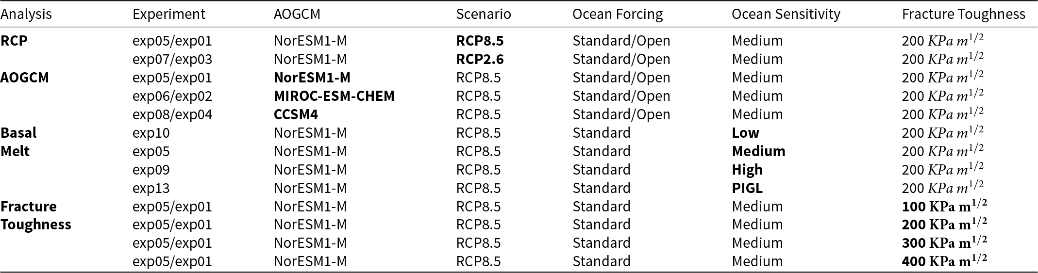


 Open access