


1. Introduction
In Antarctic coastal regions, landfast sea ice (fast ice) forms a stationary ice cover attached to the shoreline, ice shelves or grounded icebergs. It stabilizes ice shelves through buttressing and surface cooling, which reduce deformation within the ice sheet system (Massom and others, Reference Massom2010). Biologically, persistent fast ice supports marine ecosystems by influencing species distribution and nutrient exchange (Nihashi and Ohshima, Reference Nihashi and Ohshima2015). For marine operations, its stability and seasonal predictability are critical for navigation and over-ice access (Fraser and others, Reference Fraser2021). Lastly, landfast ice regulates energy fluxes at the ocean–atmosphere interface, affecting local atmospheric conditions and contributing to larger-scale climate feedbacks (Achter and others, Reference Achter2022).
The snow mass balance in coastal Antarctica is shaped by unique conditions of snow accumulation and redistribution. Studies show that blowing snow often reshapes snow cover on landfast ice, where snow depths are typically shallow (Lei and others, Reference Lei, Li, Cheng, Zhang and Heil2010; Fraser and others, Reference Fraser2023). Specifically, icebergs influence snow distribution over Antarctic fast ice through various physical processes. Wind dynamics around icebergs generate localized turbulence, resulting in large snowdrifts and uneven snow distribution on the ice (Fraser and others, Reference Fraser2023; Franke and others, Reference Franke2025). In addition, the size and mass of icebergs create shading effects, impacting solar radiation absorption and consequently affecting snowpack melting and refreezing (Nihashi and Ohshima, Reference Nihashi and Ohshima2015). Such processes collectively drive the metamorphism of snow grains, which strongly affects the insulation of the snow cover and, as a result, the thermal behavior and summer melt patterns of the ice (Zhao and others, Reference Zhao, Cheng, Vihma, Lü, Han and Shu2022). Despite their evident effect on the fast ice snow cover, mechanisms by which icebergs alter wind patterns and, in turn, drive snow redistribution remain largely unexplored.
Franke and others (Reference Franke2025) used airborne ultra-wideband microwave (UWBM) radar and laser scanner observations, among other datasets, to study icebergs embedded in fast ice. Their findings reveal persistent snow patterns around icebergs, including thick windward accumulations, elongated lateral drifts aligned with prevailing winds and nearly snow-free, rough ice surfaces in the lee. Increased cross-polarized backscatter in the UWBM data further indicates that snow loading induces basal flooding and slush formation beneath the drifts. Building on their work, the present study examines how icebergs influence wind dynamics and the subsequent effects on snow distribution. Key knowledge gaps concern the role of iceberg size and shape in controlling snowdrift formation, as well as the impact of wind conditions on accumulation patterns and volumes. Previous studies on snow accumulation around obstacles suggest that turbulence and obstacle geometry are critical factors (e.g. Tabler, Reference Tabler1980; Tominaga and others, Reference Tominaga, Mochida, Murakami and Sawaki2008), but their influence in iceberg-dominated environments remains poorly understood.
Aeolian snow transport can be classified into four modes: creep, saltation, suspension and preferential deposition (Lehning and others, Reference Lehning, Löwe, Ryser and Raderschall2008). Creep involves the sliding of particles along the surface, while saltation describes their ballistic trajectories 10–15 cm above ground. Saltating particles are set in motion through turbulent airflow (aerodynamic entrainment), collisions with other snow grains (splash) or by bouncing off the surface (rebound). Suspension occurs when lighter particles are carried by the wind over long distances, reaching heights of 0.1–100 m. Preferential deposition is the result of wind altering snowfall trajectories, leading to uneven snow distribution. Wind speed determines the dominant snow transport process, with saltation giving way to suspension as winds intensify (Gromke and others, Reference Gromke, Horender, Walter and Lehning2014).
Given the diversity of snow transport modes and their complex interactions with obstacles, predicting snow distribution in real-world conditions remains highly challenging. Snow modeling frameworks are especially useful by enabling detailed analyses of flow and snow parameters. Extensive experimental and theoretical research has been carried out to develop parameterizations for snow transport over flat terrain (e.g. Pomeroy and Gray, Reference Pomeroy and Gray1990; Doorschot and Lehning, Reference Doorschot and Lehning2002; Comola and Lehning, Reference Comola and Lehning2017), which were later integrated into numerical models (e.g. Groot Zwaaftink and others, Reference Groot Zwaaftink, Mott and Lehning2013; Sharma and others, Reference Sharma, Comola and Lehning2018). These foundational studies paved the way for developing numerical models that integrate structures into wind–snow simulations (Tominaga, Reference Tominaga2018). Two common approaches in multiphase computational fluid dynamics are the Eulerian–Eulerian (E–E) and Eulerian–Lagrangian (E–L) methods. The E–E method solves continuum equations for both fluid and particle phases, whereas the E–L method treats fluid as a continuum and tracks individual particles or particle groups along discrete trajectories. While E–E frameworks are more computationally efficient, the E–L method offers superior resolution of particle–fluid momentum exchange and near-surface dynamics, crucial for resolving snow patterns (Beyers, Reference Beyers2004; Wang and Huang, Reference Wang and Huang2017). This approach has been applied in earlier snowdrift studies to isolate the influence of individual driving factors (Hames and others, Reference Hames, Jafari, Köhler, Haas and Lehning2025). In light of its advantages, the E–L method is used in this study.
This research quantifies the influence of iceberg size and wind conditions on snow distribution around Antarctic icebergs embedded in fast ice, using the Eulerian–Lagrangian snow transport model snowBedFoam (Hames and others, Reference Hames, Jafari and Lehning2021). The objectives are as follows: (1) to assess how changes in wind conditions influence simulated snowdrift patterns and their agreement with observed snow distribution around icebergs; and (2) to explore the scaling relationship between iceberg size and snowdrift extent as well as its implications. Following its earlier use over Arctic sea ice (Hames and others, Reference Hames2022) and at an Antarctic research station (Hames and others, Reference Hames, Jafari, Köhler, Haas and Lehning2025), snowBedFoam is used here for the first time to simulate snowdrift formation around icebergs grounded in landfast ice, leveraging its ability to resolve microscale snow dynamics around complex bodies. Despite challenges of iceberg topography and the high computational cost of resolving their full scale, a successful E–L setup was achieved. A digital elevation model (DEM) from an airborne field campaign in East Antarctica (Haas, Reference Haas2023) provides the simulation topography and serves for comparison with model outputs. Using this setup, we simulate a range of iceberg sizes and wind forcing scenarios to assess their qualitative and quantitative effects on snow accumulation. This work is organized as follows: first, the data and the approach used to identify icebergs and snowdrifts are presented, followed by a description of the snow transport model. Then, results focusing on wind forcing and iceberg size are discussed, along with broader implications and conclusions.
2. Data
Extensive measurements of landfast sea ice and snow thickness, along with platelet ice occurrence and depth, were conducted along the coast of Dronning Maud Land during the ‘Antarctic Sea Ice: Thickness, Melt Ponding, and Ice Shelf Interaction’ (ANTSI) airborne campaign in November–December 2022 (Haas, Reference Haas2023; Franke and others, Reference Franke2025). Part of the surveys were carried out over landfast ice of Atka Bay (Fig. 1a), a prominent embayment about 25 km wide and up to 20 km long in the Ekström Ice Shelf, at approximately  $8^{\circ}$ west. Located near the German research station Neumayer III (Wesche and others, Reference Wesche2016), the bay typically hosts icebergs of various sizes and shapes.
(a) Location of Atka Bay in Antarctica (red square). (b) Digital elevation model of Atka Bay featuring landfast sea ice and icebergs. Elevations are given as WGS84 ellipsoidal heights. The white numbers (1–4) and ellipses display the locations of icebergs shown in the bottom panel. The dominant wind direction is from right (east) to left (west). (c) Icebergs selected for the model runs. The maximum horizontal extent is marked by the dotted arrows. Note that the dimensional scale is not respected here.

Here, we use DEMs derived from airborne laser scanner measurements of the ANTSI campaign to retrieve sizes and shapes of icebergs along with their associated snowdrifts (Fig. 1b). The airborne laser scanner system used was a RIEGL LMS-VQ580 laser scanner operating at a near-infrared wavelength of 1064 nm, with a scan angle of  $60^{\circ}$. To achieve high spatial resolution in the surface reflection point clouds, surveys were conducted at an altitude of approximately 360 m. Due to limited swath width, complete mapping of the bay was infeasible; therefore, closely spaced survey lines targeted the largest icebergs and their snowdrifts (Fig. 1b). Data processing included correction for aircraft altitude and attitude variations using GNSS and IMU data, projection of the DEM onto the WGS84 ellipsoid and adjustments of small elevation differences between swaths (Hutter and others, Reference Hutter2023; Franke and others, Reference Franke2025). Eventually, a DEM with a grid resolution of 1 $\times$1 m and an accuracy of ellipsoidal heights of 0.05 m was generated and served as a numerical base for the snow transport simulations.
The final DEM includes 33 icebergs (Fig. 1b), of which 25 were analyzed in more detail (see Methods, Section 3.1). Four of these were subsequently selected for the modeling analysis (numbered 1–4 in Fig. 1c). Icebergs were chosen for their diverse shapes, ranging from round (Iceberg 4) to elliptical (Icebergs 1 and 3) to triangular (Iceberg 2), with both flat and curved windward and lateral faces.
Atka Bay experiences very steady wind conditions with dominant easterly winds (80– $100^{\circ}$) occurring on approximately 45% of days, with an average wind speed of 8.3 m s $^{-1}$ (Klöwer and others, Reference Klöwer, Jung, König-Langlo and Semmler2014). Such conditions shape the snowdrifts into stable features, making them suitable for study and replication in numerical models. This scenario reduces the number of simulations required to replicate the drift patterns and allows for studying the cumulative consequences of wind redistribution, which would otherwise be blurred.
3. Methods
3.1. Snowdrift and iceberg retrievals
Icebergs were detected in the DEM using a combination of gradient- and elevation-based thresholding. For both parameters, the threshold was defined as  $\mu + \sigma$, where $\mu$ and $\sigma$ represent the mean and standard deviation of either gradient or elevation, consistent with standard outlier detection. First, areas with sharp elevation changes—typically marking iceberg edges—were identified using gradient magnitude analysis. These initial detections were further refined by applying an elevation threshold, preserving only regions satisfying both criteria. This approach enables the inclusion of areas with substantial elevation change while excluding low-relief regions likely associated with snowdrifts or minor terrain features. Further morphological operations were applied to refine iceberg contours, supplemented by geometric filters based on compactness and aspect ratio, resulting in an initial selection of 33 icebergs. Subsequently, eight icebergs were excluded based on the following criteria: (1) overlapping snowdrifts, (2) highly irregular or fragmented shapes and (3) insufficient size, making distinction between icebergs and their associated snowdrifts difficult. This final screening yielded 25 icebergs for analysis, of which 4 were selected for numerical modeling. Details on the horizontal dimensions, heights and representative shapes of selected icebergs are provided in Fig. A1.
Leeward regions of icebergs were found to be virtually snow-free, as indicated by the presence of rough ice across multiple measurement datasets (Franke and others, Reference Franke2025). These snow-free surfaces were used to define a zero-snow level in the DEM, from which all positive elevation differences (excluding iceberg topography) were interpreted as snow accumulation. Assuming that snow in Atka Bay is generally level in the absence of pressure ridges or icebergs, with an average thickness of 0.8 m (Arndt and others, Reference Arndt, Hoppmann, Schmithüsen, Fraser and Nicolaus2020), we identified statistically significant snow deposition zones around icebergs and analyzed their relative locations and dimensions. First, regions prone to snow accumulation were outlined using elliptical zones centered on each iceberg and aligned with the prevailing wind direction. The dimensions of these ellipses were set proportional to the square root of the iceberg’s area, such as  $a = 3 \cdot \sqrt{Area}$ and $b = 2 \cdot \sqrt{Area}$, where $a$ is the semi-major axis and $b$ the semi-minor axis of the ellipse. Icebergs were then masked out to isolate adjacent terrain. Subsequently, height anomalies within each ellipse were detected using a z-score threshold, where $z$ is defined as $z = ({x - \mu})/{\sigma}$ with $x$ the observed value, $\mu$ the mean elevation and $\sigma$ the standard deviation of surface elevation within that ellipse. A threshold of $z \gt 1$ was used to isolate areas of pronounced snow accumulation in the DEM. Similarly, we applied this approach to analyze snowdrifts in the numerical results, using preliminary ellipses and snow distribution values with $z \gt 1$ to inform the analysis. Snowdrifts retrieved with the method above provide a basis for comparing model output with measurement data. For easier comparison, the snowdrift structure was sorted into distinct regions based on their position relative to the wind (windward, leeward or lateral). Although DEM-based snow accumulation retrievals do not provide exact snow depth measurements, they adequately capture statistically significant deposition zones and allow characterization of their size, shape and spatial distribution for use in this study.
3.2. Snow transport model
Numerical experiments in this study were performed using the snow transport model snowBedFoam (Hames and others, Reference Hames, Jafari and Lehning2021). Here, it is extended to iceberg-scale structures for the first time, with new numerical challenges from the increased model scale and the complex ice topography. snowBedFoam is a fluid dynamics-based drifting snow model extended from the discrete phase model solver in OpenFOAM (The OpenFOAM Foundation, 2021). It simulates interactions between a continuous fluid phase and discrete particles using the Eulerian–Lagrangian approach (Fernandes and others, Reference Fernandes, Semyonov, Ferrás and Nóbrega2018). Given its presentation in earlier publications (Sharma and others, Reference Sharma, Comola and Lehning2018; Hames and others, Reference Hames2022; Melo and others, Reference Melo, Sharma, Comola, Sigmund and Lehning2022), we provide only a brief overview of the snow transport model used in the simulations.
In snowBedFoam, the implemented equations parametrize the three main modes of snow saltation initiation: lifting by wind shear (aerodynamic entrainment), bouncing upon impact with the surface (rebound) and ejection caused by collision with other grains (splash). Erosion of particles by aerodynamic entrainment is computed using Bagnold’s shear stress threshold (Bagnold, Reference Bagnold1941) and a parametrization by Anderson and Haff (Reference Anderson, Haff, Barndorff-Nielsen and Willetts1991), both originally developed for sand. Rebound entrainment is modeled using a rebound probability approach developed by Anderson and Haff (Reference Anderson, Haff, Barndorff-Nielsen and Willetts1991) and adapted to snow based on the work of various authors (Doorschot and Lehning, Reference Doorschot and Lehning2002; Groot Zwaaftink and others, Reference Groot Zwaaftink, Mott and Lehning2013). Equations for splash entrainment (Comola and Lehning, Reference Comola and Lehning2017) are conditioned by bed cohesion, particle diameter and velocity, particle ejection angles and impact energy (momentum) fractions. Together, these parameterizations govern the exchange of snow particles between the surface and the air, resulting in snow distribution patterns shaped by airflow, iceberg geometry and particle transport dynamics.
We employed the finite volume method to discretize the governing equations in our simulations (Moukalled and others, Reference Moukalled, Mangani and Darwish2015). The Navier–Stokes equations describe the dynamics of viscous fluid flow, accounting for momentum conservation, pressure and body forces. We used a statistically steady representation of a neutrally stratified turbulent flow by solving the Reynolds-Averaged Navier–Stokes (RANS) equations (Pope, Reference Pope2000). The Reynolds stress tensor was calculated using the standard two-equation closure model k– $\epsilon$ (Launder and Spalding, Reference Launder and Spalding1974), which solves two additional transport equations for turbulent kinetic energy (k) and turbulent dissipation rate ( $\epsilon$). Temporal derivatives were treated with a first-order implicit Euler scheme. Spatial gradients were discretized using Gauss linear interpolation. Convective fluxes in the momentum equations were evaluated with a bounded Gauss linear upwind scheme based on the local velocity gradient, while the diffusive (Laplacian) terms were discretized using a Gauss linear corrected scheme. The flow time step was automatically controlled using the ‘adjustableRunTime’ approach available in OpenFOAM, which adapts the time step based on the maximum Courant number (The OpenFOAM Foundation, 2025b).
In snowBedFoam, movement of snow particles within the domain is modeled using the Lagrangian particle tracking method. For computational efficiency, particles from the same splash event or location are grouped into parcels of similar size and trajectory. Eulerian quantities at each parcel’s location are linearly interpolated based on inverse distance weighting. Computed from gravity and fluid-particle drag forces, parcel motion is tracked using the ‘face-to-face algorithm’, which adjusts the Lagrangian time step as particles cross cell boundaries. Initially, particles are introduced into the domain via aerodynamic entrainment. Once snow parcels are aloft, the rebound-splash module is activated whenever a parcel impacts the surface, resolving the micro-scale ejection of grains from the snowbed.
3.3. Numerical settings
Figure 2a shows an example of the numerical domain used in the simulations, with Iceberg 3 as a reference. Extents of the domain in the longitudinal ( $x$), lateral ( $y$) and vertical ( $z$) directions were defined based on guidelines proposed by Franke and others (Reference Franke, Hellsten, Schlünzen and Carissimo2007), which relate domain dimensions to the maximum height (H) of the simulated object. Maximum heights of the four icebergs are 35 m (Iceberg 1), 28 m (Iceberg 2), 24 m (Iceberg 3) and 39 m (Iceberg 4). The extent of the modeled icebergs in all directions is reported in Table A2 (Appendix). In the longitudinal direction, the domain extends 8H upstream for the approach flow and 20H downstream to capture the wake region behind the iceberg. In both the lateral and vertical directions, a distance of 5H separates the iceberg from the domain walls. The chosen extents are considered sufficiently large to minimize the influence of domain boundaries on the flow around the iceberg. Simulations were conducted using an unstructured grid with a predominance of hexahedron cells. Various mesh sizes were tested, and the final configuration was selected based on computational efficiency and result consistency with finer grids. Each test result was compared to field measurements to ensure simulated patterns aligned, which led to the final mesh resolution of 2 m in the far-field and a refinement of 0.5 m near the ground and iceberg walls. As a result, the total cell count ranges from 14.5 to 43 million, depending on the shape and dimensions of the iceberg. The different iceberg sizes in Fig. 2b were modeled by uniformly scaling the reference meshes to the desired dimensions, resulting in lateral iceberg extents ranging from 125 to 1500 m.
(a) Numerical domain and boundary conditions for the snowBedFoam simulations. Labels within colored boxes correspond to the fluid phase, while conditions inside the circles refer to snow particles. Wind blows from left to right. (b) Relative scale of the five iceberg sizes tested in the simulations. The size is defined by the length of the maximum horizontal dimension, as shown in the colored rectangles at the bottom of the figure.

Detailed values for model coefficients as well as wind and snow particle properties are provided in Table A1 (Appendix). The boundary conditions set in the simulations are shown in Fig. 2a for the fluid and particle phases. At the inlet (pink), height-dependent profiles of velocity and turbulence parameters ( $k$,
$k$,  $\epsilon$) were applied, based on a generalized neutral atmospheric boundary layer profile. Profile calculations, linked to the $k-\epsilon$ model and introduced by Richards and Hoxey (Reference Richards and Hoxey1993), take the wind speed vector at a height of 10 m as an input parameter. Representative values were applied for wind speed, while wind direction was inferred from drift measurements, consistent with previous studies at the site (Klöwer and others, Reference Klöwer, Jung, König-Langlo and Semmler2014). At the outlet patch (purple), a pressure outlet condition was applied to define the pressure at the boundary, while a zero-gradient condition was used for other variables. At the side patches (light green), zero-gradient conditions were applied to all variables, which is appropriate for open domain sides where flow influence is negligible. No-slip boundary conditions were used for the velocity at the snowbed (teal) and iceberg patches, while zero-gradient was used at the top boundary. Turbulent quantities and turbulent viscosity ( $\nu_t$) at the ground were constrained with wall functions specific to the atmospheric boundary layer and consistent with the inlet condition according to the work of Hargreaves and Wright (Reference Hargreaves and Wright2007). The $\nu_t$ values were calculated using standard rough wall functions based on the aerodynamic surface roughness $z_0$ (The OpenFOAM Foundation, 2025a). Regarding particles, the aerodynamic entrainment and rebound-splash modules were enabled for the snowbed (ground) patch only. Snow surface properties are represented by the bed cohesion parameter in the model ( $\phi$; Table A1), which we set to the lower bound of the range investigated by Comola and Lehning (Reference Comola and Lehning2017). At the iceberg walls, particles were set to rebound, while they exited the domain at the lateral and top boundaries.
All simulations were initialized with fully developed Eulerian flow fields obtained after 100 s of flow-only simulation. These steady-state wind fields were then employed as initial conditions for the subsequent E–L simulations. Simulations were run until the system’s total mass stabilized, signaling steady-state erosion and deposition. This occurred in all cases by 300 s, which was set as the final simulation time.
3.4. Model runs
Rather than modeling snowdrift formation across the entire Atka Bay, we selected four representative icebergs to reduce computational demand and complexity associated with the meshing process. Each iceberg was simulated under varying wind conditions to assess its impact on snowdrift structure and to compare results to the DEM, with a focus on spatial snow distribution. Table 1 presents a typical set of simulations associated with Iceberg 1, while a comprehensive overview covering all selected icebergs is provided in Table A2 (Appendix). The generic run name begins with the iceberg identifier as defined in Fig. 1 (‘icb’), followed by its size classification (‘size’), the wind speed (‘ws’) and wind direction (‘wd’). The first bold row corresponds to the simulation with the original iceberg dimensions (size 1), a wind speed of 10 m s $^{-1}$ and a perpendicular wind direction inferred from the drift patterns ( $0^{\circ}$ in our reference system). The subsequent rows correspond to variations in wind speed, wind direction and iceberg size. The wind direction results (run wd5) are derived from averaging two runs, each with opposing $5^{\circ}$ deviations from the longitudinal axis. Combining wind directions is intended to compensate for the limited ability of the RANS model to resolve lateral variations in wind direction, such as those caused by large-scale turbulence. Simulations at wind speeds of 10 and 15 m s $^{-1}$ (ws10, ws15) were included in the analysis. Additional runs at a lower wind speed (5 m s $^{-1}$) were conducted but are not shown, as they produced very limited snow redistribution. Although higher than the regional mean wind speed (8.3 m s $^{-1}$; Klöwer and others (Reference Klöwer, Jung, König-Langlo and Semmler2014)), 10 m s $^{-1}$ represents the lower bound of typical easterly winds in the region and reliably initiates sustained snow transport in our simulations. While less frequent, 15 m s $^{-1}$ winds still occur regularly and play an important role in snow redistribution by generating more extensive snow transport.
Model runs performed for Iceberg 1, with the reference simulation highlighted in bold. Wind directions are relative to the longitudinal axis of the domain ( $0^{\circ}$). A detailed table containing simulation settings for all icebergs is provided in the Appendix (Table A2).

Alongside wind-effect simulations, iceberg dimensions were numerically modified to investigate the effect of iceberg size on snow accumulation. Variations in object size are expected to alter turbulence characteristics, with corresponding effects on snow transport dynamics. Size classes are defined based on lateral iceberg dimension (Y) as follows: 1—reference size, 2—125 m, 3—375 m, 4—750 m and 5—1500 m. These values stem from the iceberg size categories described by Orheim and others (Reference Orheim, Giles, Moholdt, Jacka and Bjørdal2022), as part of the SCAR (Scientific Committee on Antarctic Research) International Iceberg Database. For each size class, iceberg dimensions were uniformly scaled using the ratio of the target to the original lateral dimension. This approach enables numerical investigation of size effects while maintaining complete control over iceberg shape. The simulations were used to establish a numerical scaling relationship between iceberg horizontal areas and resulting snowdrift areas. This relationship was subsequently compared with its observational counterpart to assess the model’s agreement with the size-dependent trends observed in the field. For computational reasons, each iceberg size was simulated under a single wind condition.
4. Results
This section presents the analysis of iceberg-induced snowdrifts based on model results and measurements. Section 4.1 evaluates the reference simulations under varying wind conditions in relation to surface elevation data, while Section 4.2 investigates the scaling relationships between iceberg area and snowdrift area.
4.1. Snowdrifts: observations versus model
Simulations at the original iceberg scale were conducted to test whether snowBedFoam captures the observed snow distribution patterns and to assess how these patterns respond to varying wind conditions. Figure 3 shows the four icebergs selected for the simulations, with observational data (DEM) presented in the first column and corresponding model outputs displayed in the three subsequent columns. The model results include, from left to right: simulations using the reference conditions (icb_size1_ws10_wd0), the average of two wind direction adjustments of  $\pm 5^{\circ}$ (icb_size1_ws10_wd5) and simulations with increased wind speed (icb_size1_ws15_wd0). Simulation outputs are oriented to match measurements, with the wind blowing from the right. To facilitate comparison, the snowdrift pattern is categorized into four distinct regions (A–D in Fig. 3), which are highlighted in bold throughout the text. Overall, snowdrift patterns around icebergs exhibit consistent characteristics: a wide, uniform snowdrift on the windward side (A); two lateral snowdrifts forming along the sides and extending downwind (B, C); and a small, localized accumulation zone positioned directly in the lee of icebergs (D).
Comparison between observations (first column) and model results for Icebergs 1–4. Terrain elevations are relative to the WGS84 ellipsoid; lowest values correspond to snow-free sea ice, while elevated regions near icebergs indicate snow accumulation. The wind flows from right to left. The second column corresponds to the reference simulations highlighted in bold in Table 1 (wind direction:  $0^{\circ}$, wind speed: 10 m s $^{-1}$). The third column shows the averaged model results for wind directions of $-5^{\circ}$ and $5^{\circ}$. The last column shows the results obtained with a higher wind speed (15 m s $^{-1}$). Color bar limits are intentionally constrained for visualization purposes; localized values may exceed the displayed maximum.

Looking at windward accumulation on the right-hand side (A), all icebergs exhibit a narrow wind scoop (i.e. a snow-free area) at their base, which is accurately reproduced in the simulations. This snow-free area shrinks with increased wind speed, bringing snow accumulation closer to the icebergs. For Iceberg 3, the snow accumulation directly contacts the iceberg in certain locations (WS: 15 m s $^{-1}$; triangle symbol), which may explain the formation of the ‘snow bridge’ observed in the data. Iceberg 4 also exhibits a distinct feature in the upper portion of zone A, where a pronounced accumulation band extends across the erosion zone (WS: 15 m s $^{-1}$; circle symbol). This feature is also reflected in the measurements, as the green elevation contour intersects the snow-free (blue) region at the corresponding location. Simulations further indicate that snow accumulation on the windward side grows with wind speed. Although the DEM integrates snowdrifts formed under multiple wind conditions, the overall extent of the drifts is expected to primarily reflect the effects of the strongest winds. At higher wind speeds (WS: 15 m, s $^{-1}$), all icebergs exhibit an upwind V-shaped snow accumulation on the windward side, reflecting flow deceleration and recirculation. This pattern is likely amplified by numerical artefacts and is expected to be much weaker—or even absent—under naturally variable winds.
Focusing on the two accumulation zones at the flanks (B, C), simulations with artificially varying wind directions produce more accumulation streaks, covering larger lateral areas, which better matches observations. To illustrate, point C lies on the drift in the DEM, and combining the two wind directions (WD:  $5/-5^{\circ}$) extends deposition streaks into this point for all icebergs, bringing the modeled accumulation nearer to the measured drift locations. Although only two wind directions of $\pm 5^{\circ}$ were tested here, natural flows would involve a broader range of directions, collectively leading to the wider lateral side drifts seen in the measurements. Regional observations indicate that the strongest easterly winds typically range from $80^{\circ}$ to $100^{\circ}$ (Klöwer and others, Reference Klöwer, Jung, König-Langlo and Semmler2014), corresponding to a variation of $\pm 10^{\circ}$ from the simulation’s longitudinal axis. Beyond directional variability, wind speed also affects lateral snowdrift patterns (WS: 15 m s $^{-1}$). An increase in wind speed leads to a more pronounced development of the lateral drifts, characterized by greater spatial spread in both the wind and crosswind directions, along with higher accumulation quantities. Downwind positions of the resulting drift patterns align more closely with those measured in the field. Notably, the accumulation observed along the upper edge of Iceberg 2 (side C, circle symbol) is well replicated by the model. Moreover, areas of erosion predicted by snowBedFoam closely match the snow-free regions observed in the measurements, suggesting that the model effectively captures the flow dynamics around iceberg edges, as observed on Iceberg 1 (circle, triangle symbols). Other remarkable features include the erosion zone at the upper edge of Iceberg 3 (circle symbol) as well as the pronounced erosion streak on the inner side of lateral drift B (square), which are also reproduced in the model at the same locations.
Lastly, accumulations in the direct lee of the icebergs (zone D) are considered. The model generally overestimates deposition in this area, especially at higher wind speeds. Although the DEM also shows snow accumulation at these locations, amounts are lower and drifts remain largely confined to the iceberg margin. In simulations with varying wind directions (WD:  $5/-5^{\circ}$), accumulation in zone D is generally limited, as erosion from one wind direction counteracts deposition from the other. Direct lee areas undergo stronger erosion (blue zone) than others, leaving snow accumulation there particularly vulnerable to removal during wind shifts. This suggests that fluctuating wind directions are likely a key factor in the limited accumulation observed in the measurements. Despite this, distinct accumulation features still emerge in lee zone D. For Iceberg 2, accumulation streaks appear just behind the leeward tip (triangle, square symbols), a pattern that is also reflected in the simulations, although with a greater spread. Similarly, for Iceberg 4, green accumulation bands at the base of the lee side show good alignment between model and measurements (square, triangle). Among all icebergs, Iceberg 3 exhibits the highest accumulation in zone D, potentially due to airflow being channeled between the two highest crest points, forming a 6 m-deep pass that accelerates the flow.
To gain a deeper understanding of flow behavior around icebergs and its influence on snow distribution, Fig. 4 presents surface friction velocity fields (subpanels a and b) and flow streamlines (subpanels c and d) around Iceberg 3 for wind direction adjustments of  $+5^\circ$ and $-5^\circ$. This comparison highlights how minor variations in wind direction influence the flow behavior around icebergs and, in turn, affect the distribution of surface friction velocity and snow. Bold numbers in the figure and the accompanying text highlight specific regions of interest in the flow field. At the windward side (2), a zone of near-zero surface friction velocity (stagnation) appears for both wind directions, whose extent decreases with increasing wind speed. This zone shifts along the iceberg face depending on the wind angle of attack, moving toward the incoming wind direction. It coincides with areas where no snow is deposited in the simulations (Fig. 3), suggesting that the flow transporting particles is deflected before reaching this region. Once at the windward side, the flow is deflected either along the iceberg’s sides (4) or over the top (3), where its acceleration depends on the local topographic features. From (3), it predominantly returns to the sides or becomes trapped within the recirculation region (1).
The upper panels of Fig. 4 reveal that zones of high (5) and low (1) surface friction velocity in the lee shift spatially depending on wind direction. These shifts reflect changes in the flow structure in the iceberg’s wake, as illustrated by the streamlines in the lower panels, which directly influence the resulting snow distribution patterns. This effect is also evident along the iceberg’s sides (4), where the high-velocity streaks in the upper panels deform and reorient depending on wind direction. Higher surface friction velocity in (4) coincides with snow erosion observed along the edges of Iceberg 3 (Fig. 3, circle symbol). The sensitivity of the flow structure to even small wind-direction changes highlights the dominant role of lateral wind fluctuations in shaping snow distribution patterns.
While simulations capture key flow responses, the overall flow structure remains shaped by the underlying model assumptions. The simulated recirculation regions in the lee are shaped by the RANS turbulence model and the imposed neutral atmospheric stability profile. Both factors tend to overestimate turbulence behind obstacles (Tominaga and others, Reference Tominaga, Okaze and Mochida2011). Under lower turbulence levels, the recirculation zone would likely be smaller, limiting snow deposition near the iceberg (see Discussion, Section 5.2).
Surface friction velocity fields and flow streamlines around Iceberg 3 simulated for wind directions of  $+5^{\circ}$ (left column) and $-5^{\circ}$ (right column). The wind direction is indicated by the white arrows. The top panels (a, b) show surface friction velocity values in m s $^{-1}$, where higher values (in red) typically correspond to zones of snow erosion. The bottom panels (c, d) display flow streamlines extracted along the dotted line at a height of 0.8 m, selected to capture representative flow behavior in the lee of the iceberg. The streamline color scheme corresponds to wind speed expressed in m s $^{-1}$, while the ground represents surface friction velocity, as in the top panels. Turbulent structures (eddies) are clearly visible in the wake of the iceberg for both wind directions.

4.2. Iceberg size effects
Measurements show that iceberg size plays a key role in controlling the extent of snowdrift formation. Figure 5 displays the scaling relationship between iceberg area and snowdrift area, combining model simulations with measurements from the 25 selected icebergs. Alternative size combinations were tested, including correlations between iceberg height or volume and snowdrift area or volume, but the area–area relationship showed the strongest correlation. Furthermore, the lower temporal variability of snowdrift area compared with volume makes it a more suitable metric for comparing short-term simulations with measurement data.
The slope of the regression lines shown in Fig. 5 are displayed in Table 2. Leeward and lateral snowdrifts are merged to avoid a separation that can be ambiguous for certain iceberg shapes. We seek to replicate the observed scaling relationship with snowBedFoam and evaluate its ability to quantitatively simulate snowdrifts. We focus on comparing the slopes of the regression lines rather than their intercepts. The measured snowdrifts formed over longer time periods and under a broader range of cumulative wind conditions than those represented in the model simulations, which are limited to a single, short-duration wind forcing (300 s). As a result, the drift areas observed in the field are more spatially extensive, making the y-intercepts of the regressions non-comparable. In contrast, the regression slopes—capturing how snowdrift area scales with iceberg area—provide a valid basis for comparison between model outputs and measurements.
Scaling relationships between iceberg area and snowdrift area, shown on a logarithmic scale. Area represents the two-dimensional projection of icebergs and snowdrifts onto a horizontal plane (at sea-ice level). Observational data are represented by solid lines and filled circles, while model results are shown as dotted lines with unfilled markers. Each symbol corresponds to a specific iceberg, with increasing numerical size indicated by the sequence of data points. The three panels display relationships between iceberg area and (a) total snowdrift area, (b) windward snowdrift area and (c) lateral and leeward snowdrift area, respectively. The corresponding regression slopes are provided in Table 2 for simulations and measurements.

Slopes and coefficients of determination ( $\mathrm{R}^{2}$) obtained from linear regressions of modeled and measurement data (DEM), detailed in Figure 5.

In Table 2, the measured data exhibit a slope below one (0.81), indicating a sublinear relationship between iceberg area and snowdrift area. In other words, as iceberg area increases, the resulting snowdrift area expands at a proportionally reduced rate. When separating measured snowdrift data into windward and lateral/leeward components, both exhibit similar trends; however, the windward drift shows a relationship that is nearer to linear (0.94  $ \gt $ 0.70). The fitted regression lines yield high coefficients of determination (R $^2$ between 0.92 and 0.97) across all measurement plots, indicating a consistent scaling relationship between iceberg areas and snowdrift areas.
The very high  $\mathrm{R}^{2}$ observed for icebergs of different forms suggests that snowdrift area is primarily controlled by iceberg size rather than shape. Therefore, to keep meshing tractable, the four icebergs described earlier were scaled to different sizes, both smaller and larger than the original (details in Table A2). Figure 6 shows the snow deposition areas for each iceberg size class, with Iceberg 3 as a representative example. Examining the windward accumulation (on the right of each subplot), it is evident that the accumulation area changes with iceberg size. For the largest iceberg (subplot d), the extent of windward accumulation is noticeably smaller. However, this scale effect is less clear for the other iceberg sizes, as the smallest iceberg (subplot a) shows reduced windward accumulation zones compared to the directly larger iceberg sizes (subplots b and c). One possible explanation is that, in the smallest iceberg case, snow particles settle earlier in the flow, before reaching the iceberg. This results in a light, uniform deposition across the domain, limiting the amount of snow that can accumulate close to the windward side. These observations are illustrated in Fig. 5b, showing the iceberg area versus windward snowdrift area. Due to the considerable scatter in the numerical data points, the fitted slope does not represent a meaningful trend and the R $^2$ value (0.32) is lower than for its DEM-based counterpart. This means that the model-based relationship between iceberg and snowdrift areas is weaker and less defined than that in the measurements. Although a subset of the data points follow a line with the same slope as the measured one, snowBedFoam generally fails to replicate the scaling relationship for windward accumulation.
Effect of iceberg size on snowdrift size, shown for Iceberg 3, with increasing iceberg dimensions to the right. Icebergs are shown at the same visual scale, allowing direct comparison of snow deposition zones (in grey) relative to each iceberg. The maximum horizontal extent (width) of the iceberg serves as reference, taking the following values: (a) 125 m, (b) 375 m, (c) 750 m and (d) 1500 m. Results are oriented similarly to the observations, with wind coming from the right.

When examining lateral and leeward snow accumulation, the model demonstrates improved performance. Figure 6 shows that as iceberg size increases, the lateral and leeward snow accumulation decreases relative to iceberg size. Lateral and leeward drifts are smaller relative to iceberg area for larger icebergs (subplot d) than for smaller ones (subplots a–c). This is supported by Fig. 5c, which shows a significant sublinear relationship for lateral and leeward snow accumulation, with the numerical slope (0.67) closely agreeing with the observed slope (0.70). The high R $^2$ (0.86) further reinforces the idea that iceberg size plays a significant role in leeward snowdrift size, which snowBedFoam was able to reproduce.
5. Discussion
This study applied the fluid dynamics-based, Eulerian–Lagrangian snow transport model snowBedFoam to investigate drifting snow patterns around Antarctic icebergs grounded in landfast sea ice. In particular, we examined how wind and iceberg size influence snowdrift formation and distribution. Here, we discuss our main findings and their broader implications.
5.1. Roles of wind conditions and iceberg size
Snowdrift measurements show a characteristic pattern: a broad deposition zone on the windward side, lateral drifts extending downwind, a small accumulation zone immediately leeward and a subsequent area that is largely snow-free. The strong agreement between modeled and measured drift patterns indicates that wind is the dominant factor shaping snow distribution around icebergs.
In particular, results show that the longitudinal and lateral development of snowdrifts, along with total accumulation, largely increase with wind speed. This aligns with prior research identifying wind speed as a governing factor in the magnitude of snowdrifts (Hames and others, Reference Hames, Jafari, Köhler, Haas and Lehning2025). Besides, model simulations show that higher velocities increase snow accumulation near the iceberg base, reducing the extent of the windward wind scoop. In other words, strong katabatic winds frequently observed in Antarctica can transport snow up to the iceberg margin, potentially forming a snow bridge if the iceberg’s shape allows (e.g. Iceberg 3). Thus, the extent of snowdrift formation is primarily controlled by the maximum wind speed at a given location, making snowdrifts a persistent and direct indicator of local wind conditions.
Focusing on wind direction, simulations with a strictly perpendicular flow led to an overestimation of snow deposition in the direct lee of icebergs. However, combining two slightly non-normal wind directions reduced deposition in this region, resulting in better agreement with measurements. This suggests that natural fluctuations in wind direction intensify erosion in the direct lee of icebergs, making the accumulated snow prone to removal during wind shifts. Consequently, wind direction also influences the longitudinal extent of snowdrifts, although this effect remains secondary to that of wind speed. Wind directional variations additionally broaden the lateral spread of snowdrifts and distribute accumulation all around the windward face, consistent with patterns observed in the DEM. Accounting for wind-direction variability in RANS numerical models helps resolve lateral flow effects and offers a promising way to improve snowdrift extent predictions at reduced computational cost.
Our findings show that the impact of grounded icebergs on sea ice varies sharply with location. Under uniform winds, repeated snow accumulation in the same areas increases snow depth and the risk of localized flooding (Franke and others, Reference Franke2025). In contrast, variable winds promote a more even snow cover, reducing excessive loading and spatial heterogeneity of the ice.
Besides wind conditions, the relationship between iceberg size and associated snowdrift extent was investigated. Log-log plots of iceberg area versus measured snowdrift area revealed a strong sublinear relationship, indicating that larger icebergs accumulate proportionally less snow relative to their size. The strong R $^2$ indicates that the overall extent of snowdrift areas is primarily determined by iceberg size, whereas iceberg shape modulates the detailed patterns of snow accumulation, as shown in Fig. 3. Several attempts were made to identify the influence of iceberg shape on snowdrift size by correlating specific shape descriptors with snowdrift extents. However, these correlations were largely dominated by iceberg size, and we could not find conclusive insights into shape effects. Future studies could aim to more clearly isolate the influence of shape on snowdrift extents, independent of iceberg size.
5.2. Modeling considerations
The fluid dynamics model captured the general snow distribution patterns and could reproduce some of the fine-scale features with notable accuracy, although differences may arise because the model simulates snow mass, while the DEM proxies snow depth. Wind-driven compaction can increase snow mass without a proportional increase in depth; this process is not explicitly represented in snowBedFoam and should be considered when comparing model outputs to the DEM.
The model also reliably reproduced the empirical scaling of lateral and leeward snowdrifts across the simulated iceberg size range. However, snowBedFoam showed less consistency for the windward components: simulated windward drift areas displayed considerable variability, with no evident scaling relationship to iceberg size. This discrepancy likely results from model limitations, including the representation of atmospheric factors and the omission of snowfall processes (preferential deposition).
Among atmospheric factors, turbulence modeling could play a significant role, since RANS averages out turbulent fluctuations and only partially resolves large-scale eddy dynamics. In particular, RANS tends to underestimate stagnation points, reducing flow deceleration on the windward side, and overestimates the size of the recirculation region behind obstacles (e.g. Tominaga and others, Reference Tominaga, Okaze and Mochida2011). Consequently, RANS simulations are expected to reduce windward deposition while overestimating snow accumulation in the lee, consistent with our model results. Large eddy simulations offer greater accuracy but are computationally prohibitive at our current simulation scale. Applying snowBedFoam with large eddy simulations to smaller obstacles and comparing it with RANS may provide useful insights and suggest directions for future research.
Alongside turbulence modeling, atmospheric stability is another factor that can influence the wake flow and resulting snow distribution. In Antarctica, the extensive ice and snow cover cools the near-surface air layer, which very often results in stable density stratification (Dice and others, Reference Dice, Cassano, Jozef and Seefeldt2023). Under such conditions, negative buoyancy and suppressed turbulence in the lee of the icebergs would likely lead to decreased snow deposition compared to the more turbulent flow in neutral simulations (Abkar and Porté-Agel, Reference Abkar and Porté-Agel2015; González and others, Reference González, Almeida and Gutiérrez2024). In addition, the suppression of vertical mixing would concentrate particles near the surface (Tomas and others, Reference Tomas, Pourquié and Jonker2016), enhancing snow deposition on the windward side and reducing the deposition potential in the lee.
Additional processes not represented in the model may also contribute to discrepancies with measurements. Preferential deposition from precipitation (Lehning and others, Reference Lehning, Löwe, Ryser and Raderschall2008) was omitted due to computational constraints, although prior studies have demonstrated its significant contribution to windward snow accumulation (Hames and others, Reference Hames, Jafari, Köhler, Haas and Lehning2025). Similarly, shading effects associated with iceberg geometry, which can influence snowpack melt patterns (Nihashi and Ohshima, Reference Nihashi and Ohshima2015), are not included in the model and may introduce further variability. Addressing these processes in future model developments is essential for improving windward accumulation predictions.
5.3. Implications and future work
We applied a detailed E–L snow model to simulate snow dynamics around large iceberg structures. The model performs well for this case, but its computational demands make it impractical for larger obstacles or broader domains. For the same reason, simulating snow distribution over extended timescales (e.g. month-long periods) is currently infeasible. Modeling snow distribution over broader spatial and temporal scales would call for meso-scale approaches with simpler parametrizations.
In line with Fraser and others (Reference Fraser2023), our model captured the localized turbulence generated by winds around icebergs, enabling detailed examination of the flow across the entire structure. Some of the identified recirculation regions were directly linked to snow deposition patterns, providing insight into how local wind dynamics and snow distribution vary with iceberg shape. Since local wind regimes govern turbulence dynamics around icebergs, their accurate characterization is crucial for assessing the lateral and longitudinal extent of snowdrifts. Incorporating a range of wind directions and observed maximum wind speeds, weighted according to their frequency of occurrence, would likely produce snow distributions most consistent with measurements.
Conversely, observations of snowdrifts offer valuable insights into regional wind patterns. Regular remote sensing measurements of iceberg-affected areas, using synthetic aperture radar (e.g., TanDEM-X), could help monitor wind patterns in remote Antarctic regions. Such time series allow the detection of changes in snow distribution over time, as snow-free areas produce distinctive backscatter signals (Franke and others, Reference Franke2025). This approach could potentially improve our understanding of coastal wind patterns and provide crucial validation data for meso- and large-scale weather models, which often lack observations in these regions. Nevertheless, such retrievals have inherent limitations. Freshly fallen snow has very low cohesion and is therefore readily redistributed by wind, whereas wind-packed snow is more resistant to transport (Sommer and others, Reference Sommer, Lehning and Fierz2018). Consequently, snow redistribution patterns are most representative of winds occurring during or shortly after snowfall.
Franke and others (Reference Franke2025) found that iceberg-induced snowdrifts significantly alter sea ice properties, leading to ice flooding and snow ice—refrozen flooded snow at the ice surface—formation at the base of the drifts. We show that fast ice regions exposed to strong persistent winds are prone to enhanced snow ice formation around icebergs. Moreover, the sublinear scaling relationship revealed here indicates a link between ice shelf calving dynamics and landfast sea ice mass balance. Specifically, the degree of iceberg fragmentation—into fewer large or numerous smaller blocks—modulates total snow accumulation for a given ice volume and directly affects the extent of impacted sea ice. On a broader scale, regional variations in iceberg size and concentration across Antarctica may serve as proxies for sea ice properties and thickness, which affect seasonal ice dynamics. Regions with few or no icebergs tend to have more uniform coastal snow and sea ice conditions, while areas with many small icebergs exhibit greater variability and heterogeneity. This effect is especially pronounced in regions with undeformed, level sea ice, where the lack of pressure ridges reduces other sources of heterogeneity in snow distribution (Langhorne and others, Reference Langhorne2023). Such insights could improve our understanding of small-scale sea ice thickness distribution near land, supporting more effective marine navigation and operational planning.
Overall, this study advances our understanding of how iceberg characteristics and wind conditions modulate drifting snow dynamics in coastal Antarctic regions. Continued model development is needed to better capture windward accumulation and to more accurately quantify snow depth distribution near icebergs. Moreover, future work should focus on expanding the measurement dataset to include iceberg-induced snowdrifts from other regions and to simulate a wider range of wind conditions. This would support a more robust quantification of the relationship between wind conditions and snowdrift extent, strengthening the potential of snowdrifts as measures of local wind patterns.
6. Conclusion
Drifting snow and its associated mass redistribution play a critical role in shaping snow cover in Antarctic coastal regions, where landfast ice is a defining feature. In this sensitive environment, icebergs alter wind and snow patterns at the sea ice surface, with cascading effects on ecological processes and fast ice mass balance. However, the mechanisms and drivers controlling snow distribution around icebergs remain largely unknown. To address this, our study examined how variations in iceberg size and wind conditions shape snow distribution, using integrated measurement data and numerical modeling. Due to computational demands, simulations are limited in spatial and temporal extent. Turbulence representation and wind variability are also constrained, yet the results remain robust for studying snow transport dynamics around icebergs. The alignment between modeled and measured snow distribution patterns suggests that drifting snow is the primary factor driving snow mass variability around icebergs. In particular, model runs show that changes around a dominant wind direction likely limit snow accumulation in the immediate lee of icebergs, where both measurements and model results reveal pronounced erosion. Simulations further highlight wind speed as a critical factor controlling the maximum extent of snowdrifts, both laterally and along the flow direction. Consequently, peak wind speed is essential for estimating the total surface area of snow cover affected by icebergs. In parallel, results indicate that larger icebergs accumulate less snow per unit size than smaller icebergs. These findings have broader implications, as the snow mass variability driven by icebergs impacts the sea ice beneath. Icebergs formed by ice shelf calving thus serve as a bridge between ice shelf and sea ice processes, with their size determining the total snow accumulation. Moreover, the sensitivity of snowdrifts to wind parameters makes them an ideal proxy of regional wind patterns. Circumpolar remote sensing observations of snowdrifts could provide valuable validation for Antarctic weather models along the coastline. Despite its limitations, this work serves as an important first step in understanding snow distribution around icebergs and their role in the snow and sea ice mass balance of Antarctic coastal regions.
Acknowledgements
We thank the AWI polar aircraft technicians Cristina Sans Coll and Clemens Gollin for their support in the field during the 2022/23 UWBM radar flights as well as the Kenn Borek flight crew Alan Gilbertson (Captain), Noah Hladiuk (First Officer) and Brad Friesen (AME). Logistical support in the field for the airborne radar campaign has been provided by Neumayer III Station (Germany) and Troll Station (Norway). Furthermore, we are grateful for the logistics support and infrastructure for the ground-based survey on Atka Bay provided by AWI and the welcoming staff at Neumayer III Station. For the ANTSI 2022/23 airborne campaign, we acknowledge support via the AWI_PA_02135 funding grant from AWI. Océane Hames was funded by the AWI ANT-LAND funding grant AWI_ANT_27. Together with Iolène Bouzdine, part of her funding also comes from the SNSF funding grants SNF 200020_215406. This work was supported by a grant from the Swiss National Supercomputing Centre (CSCS) under project ID s1308 on Alps. Finally, the authors thank Mahdi Jafari for his input on the modeling work, as well as Steven Franke for constructive discussions on snowdrifts over landfast sea ice.
Appendix A
Plan-view geometry and height distribution of the 25 icebergs used in the analysis. Each ellipse represents one iceberg, with L $_x$ and L $_y$ denoting the plan-view length and width extracted from the DEM. The color of each ellipse indicates the 95th-percentile surface height Z $_{95}$, while the aspect ratio reflects the actual plan-view shape of the iceberg (elongated, compact or intermediate). The top inset shows an enlarged view of the smaller icebergs (Lx $ \lt $200 m and Ly $ \lt $200 m), for which height variations are less visible at the scale of the full dataset.

Model parameters, coefficients and boundary conditions used in the snowBedFoam simulations.

Model runs performed for Icebergs 1–4, with the reference simulations highlighted in bold. The dimensions have been rounded for simplicity.


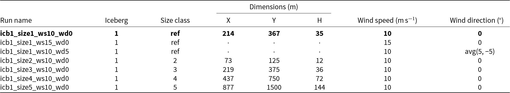


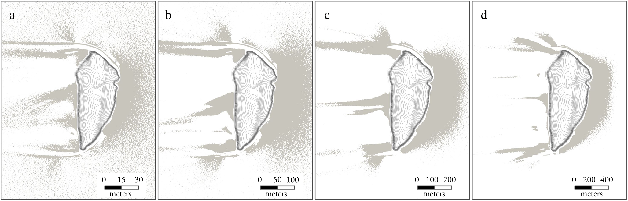


 Open access