


Nomenclature
- $a_{1x},\, a_{2x},\, a_{3x},\, n_{1}$
-
relative coordinates of the mechanism nodes, mm
-
$c$
-
airfoil chord length, mm
-
$CL$
-
lift coefficient
-
$CD$
-
drag coefficient
-
$E$
-
Young's modulus, MPa
-
$F$
-
actuator force, N
-
$G$
-
shear modulus, MPa
-
$J$
-
cost function
-
$J_1$
-
cost function computed at the free edge of the leading edge
-
$J_2$
-
cost function computed at the mechanism section of the leading edge
-
$J_3$
-
cost function computed at midsection between the mechanisms of the leading edge
-
$n$
-
number of control points on an airfoil section
-
$pos$
-
coordinate position of a control point
-
$t$
-
ply thickness, mm
-
$x,\, y,\, z$
-
Cartesian coordinates, mm


Greek symbols
-
$\alpha$
-
angle of attack, deg
-
$\delta$
-
mean absolute deviation
-
$\alpha_1, \alpha_2, \alpha_3, \theta_1, \theta_2$
-
angular orientation of mechanism rods, deg
-
$\Delta\theta_1$
-
additional rotation angle of the mechanism, deg
-
$\rho $
-
density, kg/m3
-
$\sigma$
-
stress, MPa
-
$\nu$
-
Poisson's ratio


Subscripts
- avg
-
average value
- best
-
minimum value for cost function
- max
-
maximum
- mean
-
mean value
- i
-
i-th control point
- low
-
lower camber
- up
-
upper camber
- target
-
target airfoil configuration
Abbreviations
- CFD
-
Computational Fluid Dynamics
- DNLE
-
Droop-Nose Leading Edge
- FEM
-
Finite Element Method
- GA
-
Genetic Algorithm
- MLE
-
Morphing Leading Edge
- MPC
-
Multi-Point Constraint
- NLF
-
Natural Laminar Flow
- PSO
-
Particle Swarm Optimization
- UAS
-
Unmanned Aerial System
- UAV
-
Unmanned Aerial Vehicle
1.0 Introduction
In the era of global warming, all industrial sectors contributing to greenhouse gas emissions are under increasing pressure to adopt more sustainable solutions from environmental, societal and economic perspectives. The aviation sector is one of the main contributors to climate change, and its impact is expected to grow as it remains one of the most challenging fields in which to achieve emission reductions [Reference Ryley, Baumeister and Coulter1]. Moreover, air traffic volume has increased by about 5% per year in recent years, and this trend is expected to continue, leading to a significant rise in air transport demand over the next two decades [Reference Asins, Landersheim, Laveuve, Adachi, May, Wacker and Decker2]. The Flightpath 2050 document by the Advisory Council for Aviation Research and Innovation in Europe (ACARE) has therefore set ambitious targets for emission reduction [Reference Karakoc, Colpan, Altuntas and Sohret3]. Since fuel consumption is directly linked to both emissions and operating costs, improving fuel efficiency remains a key objective for sustainable aviation [Reference Bashir, Longtin-Martel, Botez and Wong4]. An additional and often underestimated aspect is that the aviation industry must adapt to climate change [Reference Ryley, Baumeister and Coulter1]. It has been shown that temperature changes and flight altitudes will lead to longer flight times and, therefore, increased fuel consumption and emissions [Reference Skeie5]. Technological innovations to reduce aircraft emissions include sustainable alternative fuels (SAF), lightweight structures and materials, and strategies for aircraft drag reduction. Recent studies have shown that in order to mitigate global temperature change, considerable technological advancements in aviation should be introduced at the earliest possible time and in conjunction with Flightpath 2050 [Reference Karakoc, Colpan, Altuntas and Sohret3, Reference Grewe, Gangoli Rao and Grönstedt6, Reference Jahanmiri7]. In this context, efforts toward more efficient aerodynamic and structural design play a crucial role. Among the available strategies, morphing wing technologies have received increasing attention due to their potential to adapt the aerodynamic shape to different flight conditions, thereby improving lift-to-drag ratio and reducing fuel consumption [Reference Yuzhu, Wenjie, Jin, Yonghong, Donglai, Zhuo and Dianbiao8, Reference Li, Zhao, Ronch, Xiang, Drofelnik, Li, Zhang, Wu, Kintscher, Monner, Rudenko, Guo, Yin, Kirn, Storm and De Breuker9]. Although there is no strict definition of ‘morphing’, this concept generally refers to structures capable of adapting their geometry to meet varying flight conditions, enhancing aerodynamic efficiency, manoeuvrability, and overall aircraft performance [Reference Bowman, Sanders and Weisshaar10]. Among the different morphing approaches, variable-camber configurations, and in particular DNLE designs, have proven to be especially promising, as they can significantly improve aerodynamic efficiency with limited mass increase [Reference Asins, Landersheim, Laveuve, Adachi, May, Wacker and Decker2, Reference Yuzhu, Wenjie, Jin, Yonghong, Donglai, Zhuo and Dianbiao8, Reference Cavalieri11]. Previous morphing-wing studies report drag reductions in the order of 2–8 % and associated fuel-burn savings up to ∼8 % under certain conditions [Reference Taylor and Hunsaker12]. While a direct fuel-burn measurement for DNLE systems is not yet widely available, the improvements in actuator load and skin smoothness obtained in the present study are expected to contribute to lower drag and thus fuel consumption. Future work could explicitly quantify this link, considering the additional mass and complexity of the morphing mechanism in a detailed design phase. In the case of unmanned aerial systems (UAS), the implementation of DNLE morphing wings offers several specific advantages. The smaller scale and lower operational loads of UAS platforms allow for greater design flexibility and reduced actuation requirements, making them ideal demonstrators for morphing technologies. Moreover, DNLE configurations can enhance aerodynamic efficiency during take-off and landing, increase endurance and improve maneuverability, features particularly beneficial for surveillance, mapping and long-endurance missions. For these reasons, UAS platforms provide a suitable and cost-effective environment to develop and validate DNLE morphing concepts before considering larger aircraft applications [Reference Cavalieri11].
In traditional aircraft design, the increase of aerodynamic lift during take-off and landing phases relies on high-lift devices such as Krueger flaps or slats in commercial/transport aircraft. The surface discontinuities introduced by these systems have been identified as a major source of noise emission [Reference Kreth, Konig and Wild13]. Adaptive leading-edge high-lift devices have successfully decreased such noise [Reference Burnazzi and Radespiel14]. Morphing high-lift systems with continuous surfaces like the droop-nose leading edge could also allow natural laminar flow (NLF) airfoils, reducing airfoil drag and potentially decreasing the aircraft’s footprint [Reference Asins, Landersheim, Laveuve, Adachi, May, Wacker and Decker2]. Unfortunately, many engineering challenges must be faced in the practical realisation of this kind of solution. First, the skin of a morphing leading edge must be designed drastically differently from traditional airfoils. The skin must bear the aerodynamic loads acting on the airfoil and guarantee the possibility of proper deformation [Reference Yuzhu, Wenjie, Jin, Yonghong, Donglai, Zhuo and Dianbiao8, Reference Cavalieri11]. Therefore, the morphing wing skin should have a high bending strain in the morphing direction and sufficient spanwise stiffness to sustain aerodynamic loads and shape maintenance. Moreover, the shape-changing should be achieved by employing small actuator forces. In the literature, these conflicting requirements often lead to the selection of anisotropic skin materials such as composite laminates with uniform or variable thickness. It is straightforward that proper skin optimisation plays a key role in the design process of DNLE wings, while different approaches have been proposed and developed by both industry and research institutes [Reference Yuzhu, Wenjie, Jin, Yonghong, Donglai, Zhuo and Dianbiao8, Reference Cavalieri11, Reference Monner, Kintscher, Lorkowski and Storm15–Reference Gaspari, Cavalieri and Ricci17].
Another crucial aspect to consider is the morphing mechanism design, which is realised following the skin optimisation. Solutions using rigid mechanisms are linked to weight and wearing issues [Reference Yuzhu, Wenjie, Jin, Yonghong, Donglai, Zhuo and Dianbiao8]. The morphing mechanism is the main cause of the wing weight increase. For these reasons, many studies have been conducted on flexible mechanisms with simpler structure designs that do not need lubrication. However, compliant mechanisms are limited in load-bearing capability and achievable deformation, and, thus far, research on such flexible mechanisms has only been conducted mainly for small unmanned aerial vehicle (UAV) applications [Reference Tong, Ge, Sun and Liu18]. Despite the growing body of research on morphing leading-edge structures, most existing DNLE design approaches rely on iterative non-linear finite element analyses within the optimisation loop, which are computationally demanding and often difficult to generalise to different configurations. In this context, the present work proposes a design methodology aimed at simplifying the DNLE development process through an easy-to-set-up and computationally efficient framework. The proposed approach provides strategies for the selection of the composite skin architecture and for the determination of the morphing mechanism parameters, combining linear FEM analyses with kinematic optimisation to identify viable design configurations without requiring non-linear simulations during the optimisation phase, while still ensuring consistency with structural constraints and realistic morphing behaviour. In this framework, this paper proposes a methodology to design a DNLE skin as the main component of the wing and evaluate the deformations and forces needed to change the airfoil’s shape. Wing manufacturing for this work would be in composite materials, which have shown a more complex behaviour than isotropic metallic materials. When compared to the literature, our findings indicate that the proposed methodology effectively addresses some of the most crucial DNLE design challenges, namely the high actuator forces required for morphing, the trade-off between skin flexibility and load-bearing capacity and the difficulty of obtaining smooth and continuous airfoil deformations. The main advantage of the proposed approach lies in its easy setup and reduced computational effort, as non-linear FEM analyses are not required within the optimisation loop but only at selected verification stages. This hybrid strategy, combining linear FEM-based evaluations with kinematic parameter optimisation, enables a reduction of actuator loads while improving airfoil smoothness and maintaining structural integrity. The methodology proposed herein provides an efficient framework for DNLE design, developed for small UAV applications and potentially useful for future investigations toward other aircraft configurations. The paper is structured as follows: after this introduction, Section 2 describes the methodologies available in the literature to model DNLE methods. Section 3 describes a case study where our methodology is applied to a fixed-wing UAV, followed by our study’s main results in Section 4. Section 5 addresses the FEM validation of our method. Section 6 discusses our results, while Section 7 concludes the paper.
2.0 DNLE design: an overview of the methods in the literature
A workflow of the DNLE design process [Reference Monner, Kintscher, Lorkowski and Storm15, Reference Contell Asins, Landersheim and Schwarzhaupt19] is shown in Fig. 1 and described in the following paragraphs.
Workflow of the DNLE design process.

2.1 Aerodynamic optimisation of the high-lift airfoil
The first step in DNLE design is the aerodynamic optimisation of the airfoil for the take-off/landing flight conditions for a certain angle-of-attack and airspeed. In cruise conditions, it is crucial to have a minimal drag and a lift coefficient so that the lift acting on the aircraft equals its weight. During the take-off and landing phases, the lift coefficient should be maximised to have a shorter required runway length. This can be achieved by increasing the airfoil camber and chord. The optimised profile at take-off flight conditions would be inconvenient at cruise conditions since a higher value of chord and camber would result in higher drag. The advantage of morphing leading edge (MLE) systems is the possibility of exploiting the two different optimised profiles at different flight phases without having surface discontinuities that are detrimental to noise emissions and drag [Reference Bashir, Longtin-Martel, Botez and Wong20–Reference Zhigang, Xiasheng, Yu, Wenjie, Daochun, Jinwu, Panpan, Qi and DA RONCH22].
2.2 Skin optimisation
For airfoil optimisation in cruise and take-off flight conditions, two geometries are considered for those flight conditions: the initial undeformed airfoil and the target airfoils, where a deformation of the airfoil geometry is obtained through morphing. During the take-off and landing phases, the initial airfoil must be deformed to match the target. As Li et al. [Reference Li, Zhao, Ronch, Xiang, Drofelnik, Li, Zhang, Wu, Kintscher, Monner, Rudenko, Guo, Yin, Kirn, Storm and De Breuker9] highlighted, the complex functional behaviour of morphing concepts and mechanisms is not yet supported by sufficiently consolidated tools and methodologies. Despite this fact, many authors apply similar methods to realise a skin capable of fulfilling the requirements of morphing deformation and air pressure resistance. A general model that serves as a good reference for rigid morphing mechanism design is described by Rudenko et al. [Reference Rudenko, Hannig, Monner and Horst23] based on Kintscher et al.’s work [Reference Kintscher, Heintze and Monner24]. This method is based on the possibility of tailoring the stiffness of a composite laminate skin along its perimeter, considering the maximum strain, target deformation and loads due to air pressure and the actuator mechanism. Employing this process makes it possible to optimise the number and orientation of plies, the position of the stringers (application sites of the actuator forces) and the direction of the actuator forces. The optimisation starts after the consideration of initial and target shapes of the airfoils has been established as a design input, as well as the load in cruise and high-lift conditions. A finite element model of a morphing leading edge is created, and non-linear analyses are conducted on both cruise and high-lift load cases. Then, an objective function is estimated by considering different terms that should be weighted by appropriate empirical values to achieve faster convergence in the solution. Objective function terms can consider deviations in the curvature, shape and structural strain. The convergence is reached when the change in the objective function after optimisation iterations is sufficiently small. At the end of the skin optimisation, the finite element model is updated with the optimised values, and then the rigid mechanism can be designed. By also accounting for the local thickness of the airfoil as an optimisation parameter, Wang and Yang proposed a two-step design method to optimise a variable stiffness-compliant composite skin and fabric’s layers layup [Reference Wang and Yang16]. The optimisation was performed through a procedure that integrated nonlinear analyses within the iteration loop, considering the discussed optimisation parameters. A reference algorithm for this kind of optimisation is shown in Fig. 2 [Reference Wang and Yang16].
Optimisation framework for a DNLE morphing system based on Ref. [Reference Wang and Yang16].

Figure 2 Long description
The flowchart illustrates the optimization framework for a DNLE morphing system. It begins with target airfoil aerodynamic loads and initial parameters for optimization. These inputs feed into a non-linear finite element model. The model's output is evaluated using an objective function. The process checks for convergence. If convergence is achieved, the optimization is complete. If not, the mechanism undergoes further optimization.
The drawbacks of this procedure are the considerable time and effort required to set up the entire problem and the computational cost of the optimisation process, as several nonlinear analyses must be performed for each variation of optimisation parameters.
2.3 Mechanism optimisation
In the case of a rigid mechanism, from the optimised skin and force acting on the stringers, it is possible to find a geometrical solution for the position of the kinematic joints and then to design the mechanism [Reference Bashir, Longtin-Martel, Botez and Wong20]. In the case of compliant mechanisms, the optimisation process is different, and some approaches have been developed by Cavalieri et al. [Reference Cavalieri11, Reference Gaspari, Cavalieri and Ricci17]. This approach used a multi-objective optimisation analysis to find an internal structure based on the distributed compliance concept [Reference Kota, Osborn, Ervin, Maric, Flick and Paul25, Reference De Gaspari, Cavalieri and Ricci26]. The structure’s stiffness was appropriately distributed so that the deformation of the structure produces the desired target shape. A promising solution for this kind of mechanism appeared in the form of a hybrid structure design by implementing rigid components such as hinges [Reference Bashir, Longtin-Martel, Botez and Wong20].
2.4 Experimental validation
To assess the feasibility of the designed DNLE system, a small section of the wing structure had to be properly tested. Usually, the first experiments were conducted without adding the aerodynamic loads to assess the correct morphing obtained using the mechanism’s action. At this stage, it was crucial to validate the FEM model by comparing the strain measurements with the simulation results. For this purpose, optical 3D measuring systems can be adopted. Also, strain gauges could have been applied to the structure along the airfoil’s perimeter. These sensors are mostly applied on the leading-edge region of the droop nose, where simulations predict the maximum strains. In the present study, experimental and simulation data were then compared, and the deviation between the two sets was assessed. In this phase, manufacturing issues regarding the laminate composite skin can lead to consistent deviations [Reference Bashir, Longtin-Martel, Botez and Wong20]. Further analysis could be performed in wing tunnels to evaluate the behaviour of the real structure under air pressure loads, low temperatures or even icing conditions. Given the limited design methodologies developed for morphing structures, it is important to highlight the relevance of the experimental validation phase to expand the knowledge behind morphing concepts [Reference Li, Zhao, Ronch, Xiang, Drofelnik, Li, Zhang, Wu, Kintscher, Monner, Rudenko, Guo, Yin, Kirn, Storm and De Breuker9].
3.0 New methodology for DNLE structural design and optimisation
3.1 Motivation of the work
For the past few years, the Laboratory of Applied Research in Active Controls, Avionics and Servoealasticity (LARCASE) team of the École de Technologie Supérieure – Québec (ETS) has been conducting several studies concerning the application of different morphing wing technologies, using the Hydra Technologies UAS UAV-S45 as a test bench. This UAV is used in Mexico for civilian protection applications, surveillance and security [Reference Bashir, Longtin-Martel, Botez and Wong4]. The UAV-S45 is powered by two engines, a 62-cc single-cylinder with 4.75 hp power, running at 7000–7500 RPM maximum with opposite turn steering, and an air-cooled 80-cc twin-cylinder engine with 6 hp power, turning at 7200–7800 RPM maximum. The front propeller has a dimension of 23 × 10 inches, while the rear propeller is 19 × 14 inches.
Potential morphing configuration capabilities of the UAS-S45 aircraft. Image source: Bashir et al. [Reference Bashir, Longtin-Martel, Botez and Wong4].

Figure 3 Long description
An illustration of a UAS-S45 aircraft with labeled morphing configurations. The image highlights various morphing capabilities: tail morphing, trailing edge morphing, winglet morphing, upper surface morphing, and leading edge morphing. Each morphing section is annotated with specific details and diagrams showing the mechanisms involved. The tail morphing section illustrates the adjustment of the tail structure. The trailing edge morphing section shows the flexible trailing edge of the wings. The winglet morphing section depicts the adjustable winglets. The upper surface morphing section highlights the adaptable upper surface of the wings. The leading edge morphing section demonstrates the flexible leading edge of the wings. The background features a landscape with clouds and land.
The LARCASE research, just to mention a few works, has covered leading and trailing edge morphing, variable tapered wingspan and variable camber morphing wings (Fig. 3) [Reference Bashir, Longtin-Martel, Botez and Wong4, Reference Kuitche, Botez, Guillemin and Communier27, Reference Elelwi, Botez and Dao28]. In particular, in the source [Reference Bashir, Longtin-Martel, Botez and Wong4], a methodology to optimise the airfoils for the UAS-S45 has been described: a DNLE morphed airfoil can be optimised for maximising both endurance (maximum CL/CD), and range (maximum CL^1.5/CD). However, in the study [Reference Bashir, Longtin-Martel, Botez and Wong4], it is assumed that the nose of the DNLE airfoil can move only in vertical direction. After the profile aerodynamic optimisation, the maximum lift coefficient varied from Clmax=1.52 for the reference airfoil to Clmax=1.69 for the droop-nose airfoil. It is worth noting that the object of this study is substantially different from that of the discussed DNLE optimisation procedure discussed above. While a morphing mechanism model has already been proposed, there is still a need for a methodology to find a suitable composite laminate wing skin to realise a desired DNLE target airfoil. In this paper, an optimisation procedure for the morphing mechanism has been proposed and developed. According to the optimised parameters it produced, the structure has been modified and analysed to assess the possible benefits of the procedure. The initial approach to address the problem is based on non-linear structural analysis, while the new methodology introduced here promises to reduce the required computational effort because a set of linear analyses is used to evaluate the correct design point, and it only requires a few non-linear analyses. In the present paper, it is assumed that a target airfoil configuration with a droop nose has already been defined after aerodynamic optimisation. The methodology we describe here addresses the problem of defining the mechanism and the wing lamination useful to obtain the target airfoil shape. Different from the aerodynamic optimisation in which the nose of the DNLE airfoil moves only in a vertical direction with respect to the unactuated shape, the structural behaviour is considered, thus allowing the movement of the nose in a vertical and horizontal direction.
3.2 Wing skin design methodology
3.2.1 Overall approach
Investigations on the leading edge airfoil and morphing mechanism provided at the start of the project concerned the design of the laminate composite wing skin characteristics to be chosen. The design parameters [Reference Koreanschi, Sugar Gabor, Acotto, Brianchon, Portier, Botez, Mamou and Mebarki29] considered for the skin are laminate plies thickness, material and plies orientation to obtain an appropriate stress distribution along the skin. The other parameter to determine is the minimum possible value of the actuator force that should be applied on the morphing mechanism to match as closely as possible the desired leading-edge target airfoil geometry.
Initially, the mechanism geometry and the original wing airfoil were schematised and imported in the MSC PATRAN/NASTRAN FEM solver, in which the structure was reconstructed and meshed. A first guess for the laminate composite characteristics (thickness, material and plies orientation) and the pressure distribution acting on the optimised profile and boundary conditions has been implemented. At the very beginning, a wing skin characterised by relatively high stiffness was considered and analysed. Successive analyses were then performed to obtain a more deformable configuration under the same applied actuation loads. For all the cases, symmetric and balanced composite laminates were preferred, as suggested by manufacturability indications [Reference Gay, Hoa and Tsai30]. For each stacking, analyses were conducted by progressively increasing the actuator force, starting from 100 N. The results were evaluated in terms of profile displacement and stress distribution on the skin. A total of seven iterations were carried out, progressively refining the laminate configuration toward higher deformability under the same loading conditions. As indicated in Table 1, the final configuration is labeled Stacking 7, denoting the outcome of these seven iterative analyses.
Omega stringer section dimensions

Table 1 Long description
The diagram illustrates the dimensions of an omega stringer section. It includes a cross-sectional view with labeled measurements: H is 5 millimeters, t is 1.5 millimeters, W is 5 millimeters, and W1 is 2.5 millimeters. The diagram also shows the relationship between these dimensions, indicating the height, thickness, and width of the stringer section.
Based on the initial estimated laminate configuration, different FEM analyses were conducted by imposing several values of applied forces on the mechanism. To ensure a cost-effective procedure, both linear and non-linear FEM analyses were conducted. For each analysis, a cost function was estimated using the control points chosen on the morphed and target airfoil geometry to assess the closeness of the two airfoils. Equation 1 gives a formulation of the cost function J, calculated as a least square estimation, in which $n$
is the number of control points on an airfoil section,
$n$
is the number of control points on an airfoil section, $po{s_i}$
is the coordinate position of the considered control point in the morphed configuration and
$po{s_i}$
is the coordinate position of the considered control point in the morphed configuration and $po{s_{i,target}}$
is the coordinate position relative to the target airfoil. The symbols appearing in Equations (1–3) are described in the text for clarity.
$po{s_{i,target}}$
is the coordinate position relative to the target airfoil. The symbols appearing in Equations (1–3) are described in the text for clarity.
 \begin{align} J = {\rm{\;}}\mathop \sum \limits_{i = 1}^n \sqrt {{{\left( {po{s_i} - po{s_{i,target}}} \right)}^2}} {\rm{\;}} \end{align}
The general formulation of the fitness function can be written in three-dimensional coordinates, as in Equation (2):
 \begin{align} {\rm{J\;}} = \mathop \sum \limits_{i = 1}^n \sqrt {{{\left( {{x_i} - {x_{i,Target}}} \right)}^2} + {{\left( {{y_i} - {y_{i,Target}}} \right)}^2} + {{\left( {{z_i} - {z_{i,Target}}} \right)}^2}} \end{align}
where: $i$
= each node belonging to a section of the airfoil;
$i$
= each node belonging to a section of the airfoil; $n$
= the number of control points for each section (156);
$n$
= the number of control points for each section (156); ${x_i}\;,\;{y_i}\;,\;{z_i}\;$
= the x, y and z coordinates of the control point ‘
${x_i}\;,\;{y_i}\;,\;{z_i}\;$
= the x, y and z coordinates of the control point ‘ $i$
’ belonging to the morphed airfoil; and
$i$
’ belonging to the morphed airfoil; and ${x_{i,Target}}$
,
${x_{i,Target}}$
, ${y_{i,Target}}$
,
${y_{i,Target}}$
, $\;{z_{i,Target}}$
= the x, y and z coordinates of the control point ‘
$\;{z_{i,Target}}$
= the x, y and z coordinates of the control point ‘ $i$
’ belonging to the target airfoil shape.
$i$
’ belonging to the target airfoil shape.
By neglecting the out-of-section plane displacements, the cost function can be described by Equation (3), which is used in the optimisation process.
 \begin{align} {\rm{J\;}} = \mathop \sum \limits_{i = 1}^n \sqrt {{{\left( {{x_i} - {x_{i,Target}}} \right)}^2} + {{\left( {{z_i} - {z_{i,Target}}} \right)}^2}} \end{align}
Some authors propose different fitness function formulations, assigning empirical weight values to the control points, thereby giving more importance to those related to critical values of air pressure acting on the airfoil [Reference Wang and Yang16]. This is done to avoid the acceptance of eventual low values of least square error, which would correspond to unacceptable deformations. However, in this study, it was decided to create a more detailed visualisation of the airfoil matching quality by simply splitting the cost function evaluation into the upper and lower airfoil camber, as described in Equations (4–6).
 \begin{align} {J_{up}} = \mathop \sum \limits_{i = 1}^{n = 81} \sqrt {{{\left( {{x_i} - {x_{i,Target}}} \right)}^2} + {{\left( {{z_i} - {z_{i,Target}}} \right)}^2}} \end{align}
 \begin{align} {J_{low}} = \mathop \sum \limits_{i = 82}^{n = 156} \sqrt {{{\left( {{x_i} - {x_{i,Target}}} \right)}^2} + {{\left( {{z_i} - {z_{i,Target}}} \right)}^2}} \end{align}
 \begin{align} J = {J_{up}} + {J_{low}}\end{align}
Flowchart of the skin optimisation procedure introduced in this research.

Figure 4 Long description
The flowchart illustrates the skin optimization procedure. It starts from a relatively high stiffness skin configuration. The process involves analyzing geometry, material properties, pressure, and force using finite element method analysis. If the deformation delta is less than the target, the skin stacking and thickness are changed. If not, the minimum cost function is estimated. The stress on the wing skin is then calculated. If the stress is too high or too low, the process loops back to change the skin stacking and thickness. If the stress is acceptable, the profile deformation matches the target, and the stress is optimized.
The control points are the nodes obtained by meshing the original section airfoils. The cost function has been evaluated in relation to three different sections of the leading edge: the free edge $({J_1}$
), the mechanism section
$({J_1}$
), the mechanism section $({J_2}$
) and the midsection between the mechanisms
$({J_2}$
) and the midsection between the mechanisms $({J_3}$
) (Fig. 4). In this paper, the average of these three cost functions is considered as the most relevant parameter with which to assess the quality of the morphing airfoil deformation (Equation (6)). Moreover, the cost function is calculated for both the upper and lower camber airfoils, as described in Equations (7) and (8).
$({J_3}$
) (Fig. 4). In this paper, the average of these three cost functions is considered as the most relevant parameter with which to assess the quality of the morphing airfoil deformation (Equation (6)). Moreover, the cost function is calculated for both the upper and lower camber airfoils, as described in Equations (7) and (8).
 \begin{align} {J_{avg}} = \frac{{{J_1} + {J_2} + {J_{3{\rm{\;}}}}}}{3} \end{align}
 \begin{align} {J_{avg\_up}} = \frac{{{J_{1\_up}} + {J_{2\_up}} + {J_{3\_up{\rm{\;}}}}}}{3} \end{align}
 \begin{align} {J_{avg\_low}} = \frac{{{J_{1\_low}} + {J_{2\_low}} + {J_{3\_low{\rm{\;}}}}}}{3} \end{align}
Another relevant parameter with which to evaluate the smoothness of the airfoil along the wingspan is the mean absolute deviation δ of the three sections considered around the average cost function value, as expressed in Equation (10). This parameter is also evaluated for both upper and lower camber airfoil (Equation (11) and (12), respectively).
 \begin{align} \delta = \frac{{\mathop \sum \nolimits_{i = 1}^3 \left| {{\rm{\;}}{J_i} - {J_{avg}}} \right|}}{3} \end{align}
 \begin{align} {\delta _{up}} = \frac{{\mathop \sum \nolimits_{i = 1}^3 \left| {{\rm{\;}}{J_{i\_up}} - {J_{avg}}} \right|}}{3} \end{align}
 \begin{align} {\delta _{low}} = \frac{{\mathop \sum \nolimits_{i = 1}^3 \left| {{\rm{\;}}{J_{i\_low}} - {J_{avg}}} \right|}}{3} \end{align}
If the displacement obtained by the results from FEM linear analyses does not reach the required displacement, another composite configuration with lower stiffness must be considered and the procedure re-iterated. The most suitable case among those analysed is the one corresponding to the minimum cost function value. This case would then be investigated in terms of stress distribution acting on the skin through non-linear FEM analyses. To assess whether the stress level in the composite skin was acceptable, a maximum-stress approach was adopted. Stress values exceeding approximately 50% of the material’s ultimate strength were considered too high, indicating an overstressed configuration, while values below about 25% of the ultimate strength were regarded as too low, suggesting that the laminate stiffness was excessive and underutilised. These thresholds were defined as engineering guidelines rather than fixed limits, since the acceptable range can vary depending on the specific composite material, the applied load conditions, and the desired safety margin. In case of a too-low or excessive stress value, a further change in the laminate composite characteristics must be made, and the procedure repeated from its beginning. At the end of this algorithm, the final obtained airfoil is the one closest to the target (using the initial mechanism design). At the same time, an optimised composite laminate skin is found in terms of displacements and the force exerted by the actuator on the mechanism. This workflow is shown in Fig. 5.
Geometrical schematisation (left) and PATRAN 3D model (right) of the morphing airfoil.

Figure 5 Long description
The image contains two elements: a geometrical schematisation on the left and a PATRAN 3D model on the right. The geometrical schematisation shows a detailed diagram of the morphing airfoil mechanism with various nodes and coordinates marked. The PATRAN 3D model presents a three-dimensional view of the airfoil, highlighting its structure and design. The two images together illustrate the design and modeling process of the morphing airfoil.
3.2.2 Structural modeling of the leading edge
Starting from the original airfoil and morphing mechanism, a 3D model of 800mm of the wing was developed, approximated as a rectangular wing. While some authors have analysed only small wing sections, each containing only one DN mechanism, in this study, the presence of two consecutive mechanisms in the same section is considered to assess their influence on the stresses and displacements in the midsection [Reference Yuzhu, Wenjie, Jin, Yonghong, Donglai, Zhuo and Dianbiao8]. For this reason, along the 3D model of the 800mm wing length, two equally spaced mechanisms were placed, with, as a first attempt, a total of six mechanisms in a single wingspan, according to Li et al. [Reference Yuzhu, Wenjie, Jin, Yonghong, Donglai, Zhuo and Dianbiao8]. The 3D wing model was imported into PATRAN 2020 to perform the FEM analyses (Figs 6 and 7).
Properties of fiber/epoxy plies – adapted from D. Gay [Reference Gay, Hoa and Tsai30]

Table 2 Long description
A table listing properties of fiber/epoxy plies for carbon material. The table includes specific mass, longitudinal tensile strength, longitudinal compressive strength, transverse tensile strength, transverse compressive strength, longitudinal elastic modulus, transverse elastic modulus, shear modulus, and Poisson ratio. The table has 10 rows and 2 columns. Row 1: Specific mass, 1,530 kilograms per cubic meter. Row 2: Longitudinal tensile strength, 1,270 megapascals. Row 3: Longitudinal compressive strength, 1,130 megapascals. Row 4: Transverse tensile strength, 42 megapascals. Row 5: Transverse compressive strength, 141 megapascals. Row 6: Longitudinal elastic modulus, 134,000 megapascals. Row 7: Transverse elastic modulus, 7,000 megapascals. Row 8: Shear modulus, 4,200 megapascals. Row 9: Poisson ratio, 0.25.
Surface model of a DNLE UAS-S45 airfoil leading edge (left), and its modelling in Patran (right).

Figure 6 Long description
The left image shows a surface model of a DNLE UAS-S45 airfoil leading edge, displaying a detailed 3D representation of the airfoil's surface. The right image illustrates the modeling of the same airfoil leading edge in Patran software. The model is divided into sections labeled as Mechanism 1, Mechanism 2, and Midsection, each separated by 200 millimeters. The free edge is also labeled, indicating the end of the leading edge. The model includes various nodes and control points, with annotations showing relative coordinates and other technical details.
Oriented stringers with no offset (left) and with offset (right).

Figure 7 Long description
The image shows two diagrams comparing oriented stringers. The left diagram illustrates stringers with no offset, while the right diagram shows stringers with an offset. Both diagrams feature a series of interconnected nodes and lines representing the structure and alignment of the stringers. The diagrams highlight the differences in the positioning and orientation of the stringers due to the presence or absence of an offset.
The wing skin material has an important role in achieving the leading-edge morphing. For this kind of application, the skin material must have a high curvature at breaking stress, and, at the same time, it must provide sufficient spanwise stiffness to withstand the aerodynamic loads, and thus to reduce the number of morphing mechanisms required. In this perspective, the selected material should have a high anisotropy [Reference Contell Asins, Landersheim and Schwarzhaupt19]. The choice of the wing skin material has been subjected to several design constraints, including being composed of a composite laminate material with the possibility to choose between commercial E-glass/epoxy, carbon/epoxy, and Kevlar/epoxy balanced fabric composite material. Without considering thickness or stacking configuration, the skin has been modelled as a 2D thin laminate shell with the orthotropic material properly oriented along the surface. The selected stringer material is a composite material composed of three plies of unidirectional carbon/epoxy, where each ply has a thickness of 0.5mm, for a total thickness of 1.5mm. A constant omega cross-section has been chosen, with its dimensions and material properties as indicated in Tables 2 and 3, respectively.
The mechanism’s material is an aluminum alloy 7075 widely used for aeronautical applications and available off-the-shelf, with a rectangular cross-section profile and characteristics; its properties and geometric profiles are indicated in Tables 4 and 5, respectively.
Aluminum 7075 properties

Table 3 Long description
The table presents the properties of Aluminum 7075. It contains four rows and four columns. The columns are labeled as Elastic modulus, Shear modulus, Density, and Poisson Ratio. The first row shows the elastic modulus as seventy-one thousand seven hundred megapascals. The second row indicates the shear modulus as twenty-six thousand nine hundred megapascals. The third row lists the density as two thousand eight hundred kilograms per cubic meter. The fourth row specifies the Poisson ratio as zero point three three.
Mechanism rectangular section geometry

Table 4 Long description
A table titled Mechanism rectangular section geometry presents the dimensions of a rectangular section. The table has three columns labeled W, H, t1, and t2, and four rows including the header. The width (W) is 4 millimeters, the height (H) is 6 millimeters, and both t1 and t2 are 1 millimeter each. The table provides a clear and concise representation of the geometric parameters of the mechanism's rectangular section.
Properties of balanced fabric/epoxy composites – adapted from D. Gay [Reference Gay, Hoa and Tsai30]

Table 5 Long description
The table presents the properties of balanced fabric/epoxy composites, specifically E-glass. It includes specific mass of 1,900 kilograms per cubic meter, tensile strength of 400 megapascals in both x and y directions, compressive strength of 390 megapascals in both x and y directions, elastic modulus of 20,000 megapascals in both x and y directions, shear modulus of 2,850 megapascals, elongation at break ranging from 2.5 to 3.7 percent, and a Poisson coefficient of 0.13.
3.2.3 Meshing
Meshes of the structure were realised within a PATRAN workspace. The surface of the LE wing skin was meshed using a curved-based mesh-seed for the side of the airfoil with a maximum allowable error equal to hmax=0.01mm. The straight sides of the surface were meshed using a uniform mesh seed. A total of 124,956 nodes and 127,200 CQUAD4 elements with dimensions of 1x1 mm were realised to mesh the wing surface. The choice of CQUAD4 elements and of the shell material was also determined by the fact that they support nonlinear analyses.
The number of nodes of each stringer is equal to the number of nodes in a single line along the spanwise direction of the considered wing. In this way, by employing the equivalence command, it is possible to place a stringer directly on the wing skin. The next step is to set an appropriate offset to the centre of mass of the stringer cross-section at each node, to guarantee a value of the inertia matrix that is more appropriate for the stringers, simulating a perfect adhesion between the stringers and the wing skin. Therefore, each stringer cross-section was oriented to follow the curvature of the skin, as shown in Fig. 4.
Some researchers have addressed this problem by creating stringers made of surface elements and then by creating a permanent glued contact between the stringers and the skin (e.g. Ref. [Reference Wang and Yang16]). The primary benefit of a permanently glued contact is that it can connect dissimilar meshes. The higher level of accuracy in the analysis of the interaction between stringers and wing skin incurs a cost in terms of model complexity. The benefits of the proposed approach are in the simplicity and flexibility of creating different stringers’ shapes and geometries, which allows for faster testing of various possible solutions. On the other hand, this approach can lead to non-convergence problems in the nonlinear analysis due to the possible high differences in stiffness between adjacent elements around the same node. However, this issue can be addressed by geometrical adjustments or by using the most suitable NASTRAN solver. In the analysis conducted using NASTRAN nonlinear solver ‘sol400’, non-convergence problems never occurred. It is important to note that NASTRAN nonlinear solvers are not allowed to conduct analyses on beam elements with non-zero offsets. Therefore, when switching from linear to nonlinear analysis, the beam elements are set up with a zero offset. The offsets between the beam elements and the reference line of the morphing mechanism are on the order of a few millimeters. Neglecting these offsets slightly reduces the structural stiffness, resulting in a marginally more compliant model. This simplification was required due to solver limitations in the nonlinear NASTRAN environment, which does not allow offset definitions under large-deformation conditions. Although this assumption introduces a minor deviation from the physical stiffness distribution, its influence on the global deformation behaviour is expected to be limited and not significant for the present analysis. Correction factors or refined modeling strategies to compensate for the zero-offset assumption could be adopted to further increase the fidelity of the model.
The mechanism has been meshed by means of BEAM elements with a uniform length of 0.5mm. The entire wing model is made of 125,386 nodes and 126,822 elements. In the original mechanism concept representation provided by the LARCASE team, the rotation of the arms around each hinge axis is allowed. To realise this kind of kinematic structure, each arm of the mechanism was properly meshed, and multi-point constraints (MPCs) between matching nodes corresponding to the hinges of the mechanism were properly realised: MPCs were set up by means of RBAR elements allowing just one degree of freedom rotation around the y-axis. The wing structure is shown in Fig. 8.
Mesh of the morphing leading edge structure on PATRAN (stringers on the left; mechanism on the right).

Figure 8 Long description
The image presents a detailed mesh of a morphing leading edge structure, divided into two sections. On the left, the mesh displays stringers, which are structural elements designed to provide strength and stability. The right section illustrates a mechanism, likely responsible for the morphing functionality. The mesh is color-coded in teal and black, highlighting different components and their intricate details. The structure is oriented horizontally, with the stringers extending along the length of the leading edge and the mechanism positioned centrally. The image provides a clear view of the internal geometry and spatial arrangement of the components, essential for understanding the design and functionality of the morphing leading edge.
3.2.4 Loads and boundary conditions
It has been shown that a significant amount of the forces exerted by a morphing mechanism is used to deflect the leading-edge skin, and to overcome the aerodynamic pressure load acting on it [Reference Kintscher, Monner and Heintze31]. Therefore, the aerodynamic pressure has been accurately modeled and implemented into the model using the tabular data of pressure acting on the skin of the droop-nose configuration airfoil, optimised at α = 6°, provided by the LARCASE laboratory. As shown in Fig. 9, the pressure distribution was considered as just the one relative to the droop-nose section, which is up to a value of x/c = 0.15. Figure 9 in the right side shows the pressure distribution on the leading edge implemented on PATRAN.
Example of pressure distribution on the optimised droop-nose airfoil (pressure distribution along the chord on the left; pressure on the surface of the leading edge on the right).

Figure 9 Long description
The left side of the image features a line graph depicting pressure distribution along the chord of an optimized droop-nose airfoil. The x-axis represents the chord length, labeled as x over c, ranging from 0 to 1.05. The y-axis represents pressure in pascals, ranging from negative 1600 to 1000. The graph shows two distinct lines, one with a steep decline and another with a gradual increase. The right side of the image displays a 3D surface plot illustrating pressure on the surface of the leading edge of the airfoil. The plot uses a color gradient to represent different pressure values, with a scale on the right ranging from negative 2.36 to negative 14.03. The plot includes a coordinate system with axes labeled x, y, and z. The surface plot shows varying pressure distributions across the leading edge, with notable changes in color indicating different pressure regions.
The actuator effect was considered by means of a force applied to the mechanism and with the same inclination indicated in Fig. 7. In each analysis, this load was modified to better realise the desired angular variation to the mechanism and to give first indications on the appropriateness of the considered wing skin thickness and stacking. As a first approximation, the leading edge can be analysed without considering the rest of the wing, as it is clamped to the wing box by means of the front spar. This approach is widely adopted in the literature. Analogously, the mechanism is rigidly connected to the front spar by employing a hinge that allows only rotation around the y-axis. The structure approximation is shown in Fig. 10.
Boundary conditions’ approximation of a morphing leading edge.

Figure 10 Long description
The image shows a diagram of a morphing leading edge with fixed boundary conditions. The leading edge is represented by a series of black dots connected by lines, indicating the mechanism nodes. The fixed boundary is depicted on the right side of the diagram with diagonal lines. The leading edge is labeled with various parameters such as relative coordinates of the mechanism nodes, airfoil chord length, lift coefficient, drag coefficient, Young's modulus, actuator force, shear modulus, cost function, number of control points, coordinate position of a control point, ply thickness, and Cartesian coordinates.
3.3 Methodology chosen for the optimisation of the morphing mechanism
3.3.1 Approach overview
Starting with the designed wing skin, the proposed mechanism’s geometry was investigated. The structure’s geometry was parameterised using ten parameters, and a MATLAB code was developed. Two assumptions were proposed: first, to treat the structure as one-degree kinematic geometry to find node positions after mechanism rotation; and second, to use a spline to interpolate displaced nodes from the undeformed airfoil geometry. Two MATLAB functions (genetic algorithm and particle swarm optimisation) optimised the code, determining the optimal parameters by minimising the airfoil’s cost function. The modified structure underwent non-linear FEM analyses under varying actuator forces. The solution with the lowest cost function was chosen, and actuator force, airfoil deformation, and stress distribution were analysed. Figure 11 presents this approach as a flowchart.
Flowchart of the mechanism optimisation procedure adopted in this study.

Figure 11 Long description
Flowchart of mechanism optimization procedure with steps and decision points. The process starts from a designed skin and proceeds through structure parameterization and assumptions. It involves the estimation of the deformed airfoil and cost function J. The optimization uses genetic algorithms (GA) and particle swarm optimization (PSO) to find optimized parameters with minimum J value. New geometry, material properties, boundary conditions, pressure, and force are then analyzed using finite element method (FEM). The minimum J case from analysis is evaluated, and if the parameters alpha, J, and F are lower, the optimized structure is achieved. If not, assumptions and optimization options are changed, and the process repeats.
3.3.2 Parametrisation and determination of the deformed airfoil
A MATLAB code was developed to parameterise the mechanism’s initial profile using ten geometrical parameters, detailed in Fig. 12. These parameters include the x-coordinates of nodes (a1x, a2x, a3x and n1), angular orientations (α1, α2, α3, θ1 and θ1), and an additional rotation (Δθ1) of the main mechanism. Initially, the mechanism’s hinge and initial profile points remain fixed. Intersection points between the mechanism and the airfoil (MPC4, 5, 6, 7 in Fig. 12) can be found by varying the first nine parameters listed above.
Parametrisation of the morphing mechanism.

Figure 12 Long description
The diagram illustrates a morphing mechanism with various labeled coordinates and components. The upper and lower chambers are marked, with control points labeled as MPC4, MPC5, MPC6, and MPC7. The coordinates a1x, a2x, a3x, and n1 are indicated, representing the relative positions of the mechanism nodes in millimeters. The angles alpha1, alpha2, alpha3, beta1, and beta2 are shown, along with the change in angle Delta theta1. The Cartesian coordinates x, y, and z are also depicted. The diagram includes annotations for the airfoil chord length c, the lift coefficient CL, the drag coefficient CD, Young's modulus E, the actuator force F, the shear modulus G, and the cost functions J, J1, J2, and J3. The ply thickness t is marked in millimeters.
To determine the deformed airfoil after a rotation Δθ1, two assumptions were made:
-
1. First assumption: The mechanism’s MPC points along the skin move as a one-degree kinematic geometry, resembling four-bar linkages. Two structural approximations were considered; each was assessed using a MATLAB code.
-
• In the initial approximation, the wing skin section was treated as three four-bar linkages, allowing precise node evaluation after Δθ1 (Fig. 13);
Figure 13.Movement of the nodes after a mechanism rotation in the first structure approximation.
Figure 13 Long description
The image presents a diagram illustrating the movement of nodes after a mechanism rotation in the first structure approximation. The left side of the diagram shows the initial positions of the nodes connected by lines of different colors, representing various structural components. The right side of the diagram depicts the new positions of the nodes after the mechanism rotation, with lines indicating the movement paths. The nodes are connected by lines of different colors, indicating the relative coordinates of the mechanism nodes in millimeters. The diagram includes labels for the nodes and their relative coordinates, as well as the airfoil chord length and other mechanical properties. The movement of the nodes is shown with arrows and lines, indicating the direction and extent of the rotation.
-
• The second approximation considered the upper wing skin as a single beam with connected rods and hinges (Fig. 14).
Figure 14.Movement of the nodes after a mechanism rotation in the second structure approximation.
Figure 14 Long description
A flowchart illustrating the movement of nodes after a mechanism rotation in the second structure approximation. The flowchart consists of two main sections, each depicting a different stage of the mechanism's rotation. The left section shows the initial positions of the nodes, represented by black dots connected by lines of various colors. The right section illustrates the positions of the nodes after rotation, with additional elements such as circles and arrows indicating movement and interaction. Key components include nodes, lines representing connections, and colored paths showing the direction and extent of movement. The flowchart highlights the relative coordinates of the mechanism nodes, the airfoil chord length, and the forces acting on the structure.
-
-
2. Second assumption: The leading edge of the deformed airfoil can be approximated by a spline passing through the displaced MPC points (Fig. 15). The airfoil was evaluated in MATLAB by means of a Catmull-Rom spline, given the position of interpolation points. The morphed airfoil was divided into 156 equally separated control points to allow the computation of the J cost function.
Figure 15.Example of a deformed profile evaluation through a spline passing through displaced nodes.
Figure 15 Long description
The diagram illustrates a deformed profile evaluation using a spline that passes through displaced nodes. The spline is depicted as a curved line connecting several nodes, which are marked with red and black dots. The diagram includes various lines and arrows indicating the direction and extent of deformation. The nodes are connected by orange and blue lines, representing different sections of the mechanism. The spline is shown in black, highlighting the path through the displaced nodes. The overall structure suggests an analysis of mechanical deformation in a specific profile.


Using the MATLAB function built according to the procedure described above, it is possible to draw the morphed shape and to evaluate the cost function for each combination of geometrical parameters and to impose an additional rotation on the mechanism. This MATLAB function has been optimised, aiming at minimising the value of the cost function J and finding the optimal values of the ten geometrical parameters defined at the beginning of Section 3.3.2. The morphing structure approximated via the two options discussed above was optimised using a genetic algorithm and then a particle swarm optimisation method. A graphical representation of the iteration shapes is shown in Fig. 16.
Stacking final configuration and thickness

Evaluation of different mechanism geometries and deformed profiles using the optimisation toolbox.

Figure 16 Long description
A scatter plot with hundreds of data points in blue and red colors representing different mechanism geometries and deformed profiles. The x-axis ranges from 0 to 60 degrees, and the y-axis ranges from 0 to 50 degrees. The data points form distinct clusters and patterns, with some points connected by dashed lines. The plot includes a legend indicating the color coding for different data sets. All values are approximated.
4.0 Results
4.1 Results of the wing skin design
A large part of the initial analyses was conducted using the linear NASTRAN solver ‘sol101’ to provide useful indications for the material and wing skin configurations, significantly reducing the computational time. The most relevant cases were analysed using the non-linear NASTRAN solvers ‘sol106’ and ‘sol400’. During the analysis, the structural parameters that were gradually modified consisted of the combination of ply thickness, material and orientation of each composite ply. The properties of the single ply are listed in Table 6. Each combination was referred to by means of the term ‘stacking’. Initially, a wing skin characterised by a relatively high stiffness was considered and analysed. Further analyses were targeted to reach a more deformable wing for equal loading applied to the mechanism. For all cases, symmetric and balanced composite laminates were preferred, as suggested by manufacturability indications. For each stacking, analyses were conducted by increasing the value of each force applied to the mechanism, from F = 50N up to F = 250N, which are reasonable values for actuators of small dimensions. The results of these analyses are expressed in terms of airfoil geometry displacement and stress distribution on the skin (see Fig. 17).
In each analysis, the maximum stresses occurred in the most external layer of the composite laminate. After seven different stacking iterations, the results of linear analyses led to a configuration made by two plies of glass/epoxy with 0.1mm thickness, oriented at ±45°each, thus having a composite laminate total thickness of 0.2mm (Table 1).
As shown in Table 7, the results obtained using the linear and nonlinear solvers are close for small values of forces (F = 50N, F = 100N), and then start to differ as the force increases more significantly. This is due to the geometrical nonlinearity linked to the lack of fulfillment of the small displacement hypothesis. This increasing discrepancy between the solutions given by linear and nonlinear solvers is consistent with analogous examples in Ref. [Reference Masud, Tham, Cheng and Gu32]. The approach adopted until this point, combining linear and nonlinear analyses, was convenient and useful, as it allowed the minimum stiffness to be reached in the wing skin while also minimising the force required to deform the airfoil shape. From Table 7, it can be observed that the force value needed to reach the same value of mechanism rotation resulting from linear analyses will be significantly higher, thus requiring more powerful actuators. The approach we followed requires focusing on finding the angular rotation of the mechanism, corresponding to a certain force applied to it, that leads the node corresponding to multi-point constraint 6 to be placed approximately on the target airfoil shape, and then evaluating the cost function for different analysed cases. The results of the sol400 nonlinear analyses conducted to find the appropriate rotation of the mechanism are presented in Table 8.
Comparison of displacement results from linear and nonlinear analyses of ‘stacking 7’ configurations

Table 7 Long description
The table compares displacement results from linear and nonlinear analyses of stacking 7 configurations. It has seven rows and three columns. The columns are labeled Sol 101 linear, Sol106 nonlinear, and Sol400 nonlinear, each showing maximum displacement in millimeters for different force values. The rows are labeled with force values in Newtons: 50 N, 100 N, 125 N, 150 N, 175 N, 200 N, and 225 N. For F = 50 N, the displacements are 1.34 millimeters, 1.10 millimeters, and 1.10 millimeters respectively. For F = 100 N, the displacements are 1.93 millimeters, 1.70 millimeters, and 1.70 millimeters respectively. For F = 125 N, the displacements are 3.43 millimeters, 2.60 millimeters, and 2.60 millimeters respectively. For F = 150 N, the displacements are 4.93 millimeters, 3.15 millimeters, and 3.15 millimeters respectively. For F = 175 N, the displacements are 6.43 millimeters, 3.50 millimeters, and 3.50 millimeters respectively. For F = 200 N, the displacements are 7.93 millimeters, 3.75 millimeters, and 3.75 millimeters respectively. For F = 225 N, the displacements are 9.43 millimeters, 3.93 millimeters, and 3.93 millimeters respectively. The table shows that the results obtained using the linear and nonlinear solvers are close for small values of forces and start to differ as the force increases more significantly.
Comparison between initial (purple) and target (yellow) leading edge geometry.

Figure 17 Long description
A line graph compares the initial and target leading edge geometry. The initial geometry is represented by a purple line, while the target geometry is shown by a yellow line. The graph includes a vertical scale marked in millimeters, with a specific measurement of seven millimeters indicated by a yellow arrow. The x-axis and y-axis are labeled, and the graph features multiple intersecting lines that illustrate the differences between the two geometries. All values are approximated.
Maximum displacement and mechanism rotation results from non-linear analyses on final stacking – original mechanism

These analyses show that to reach an angular rotation of the mechanism between 5.5° and 7°, the force values range from 1000N to 2250N, thus requiring more powerful actuators, with increasing sizes and masses. This aspect is significant, as the actuator’s size is restricted by the small area available inside the wing airfoil. It is worth noting that none of the deformed airfoils from the analyses perfectly match the target profile. The determination of the most appropriate deformation amongst those analysed was assessed by means of the cost function, with the results presented in Table 9. The best load condition and consequently the best value of angular rotation of the mechanism among those analysed has the force value of 1000 N, which gives the minimum value of the cost function ${J_{avg}} = 149.65$
, and a mechanism rotation of about 5.5°.
${J_{avg}} = 149.65$
, and a mechanism rotation of about 5.5°.
Cost function values from FEM nonlinear analyses on optimised skin for the original mechanism

Table 9 Long description
A table with seven rows and six columns presents cost function values from finite element method nonlinear analyses on optimised skin for the original mechanism. The columns are labeled J1, J2, J3, Javg, Javg_up, and Javg_low. The rows correspond to different force values ranging from 800 newtons to 2000 newtons. Each cell contains a numerical value representing the cost function at specific force levels. Notable trends include increasing cost function values with higher force levels, with the lowest average cost function value of 149.65 occurring at 1000 newtons and the highest at 2000 newtons with a value of 203.29.
The stress distribution is illustrated in Fig, 18. Figures 19 and 20 show that the deformation imposed on the airfoil by the original LARCASE mechanism does not reach the desired target airfoil. Thus, the initial mechanism configuration can be further improved. For this reason, the methodology described in Section 3.3 was applied to refine the structural layout and mechanism geometry: this in order to better approach the target DNLE shape. As will be described in Sections 4.2 and 4.3, the optimised configuration leads to a significantly improved matching of the desired profile; however, even at the end of the optimisation, a perfect correspondence is still not achieved. It’s important to note that the approach described in this paper assumes a target airfoil with a drooping nose shape is available from aerodynamic analysis, and the goal is to design a structural configuration that can reproduce, at best, the target DNLE airfoil.
Stress distribution along the most external layer of the skin from non-linear analysis at F = 1000N – Final stacking.

Figure 18 Long description
A heat map displays stress distribution along the most external layer of the skin from non-linear analysis at a force of 1000 Newtons Final stacking. The heat map uses a color scale ranging from blue to red, indicating varying stress levels. Blue areas represent lower stress, while red areas indicate higher stress. The stress values range from approximately 2.55 to 150 megapascals. The heat map shows a gradient of stress distribution, with higher stress concentrations in specific regions and lower stress in others. The overall structure of the heat map is elongated, with distinct areas of varying stress intensity.
MATLAB profile displacement at different sections of the wingspan – results of FEM non-linear analysis at F = 1000N – Final stacking.

Figure 19 Long description
The line graph compares airfoil profiles at different sections of the wingspan from FEM non-linear analysis at a force of 1000 newtons. The x-axis represents the position along the wingspan in millimeters, ranging from 0 to 60 millimeters. The y-axis represents the vertical displacement in millimeters, ranging from 0 to 50 millimeters. The graph includes five data series: initial airfoil, target airfoil, actual airfoil at the free edge, actual airfoil at the mechanism, and actual airfoil at the midsection. Each data series is represented by different markers: plus signs for the initial airfoil, red dots for the target airfoil, blue circles for the actual airfoil at the free edge, black circles for the actual airfoil at the mechanism, and green circles for the actual airfoil at the midsection. The data points show the displacement profiles of the airfoils at various sections along the wingspan. All values are approximated.
4.2 Results of the optimisation of the morphing mechanism
For both GA and PSO, the initial population range was set, and the entire population was lower- and upper-bounded using the values shown in Table 10.
The optimisation parameters were set as follows:
-
• GA: population size = 120; maximum iterations = 300
-
• PSO: population size = 120; maximum iterations = 300
GA optimisation results
GA optimisation was performed on both approximated structures, as shown in Figs 14 and 15. The population dimension considered is equal to 120. Reproduction, mutation, crossover and migration options were set to the default values of the MATLAB @ga function. In the first approximated structure (Fig. 14), the optimisation ended after 141 generations when the average change in the fitness value was less than its default option. The minimum cost function value was Jbest = 88.24, with mean value Jmean= 93.22. The optimised parameters are shown in Table 11. These values were compared to those of the original structure, where Jbest was evaluated using the above-described MATLAB code.
In the second approximated structure (Fig. 15), the optimisation stopped after 281 generations, when the time limit set for the process was reached. The minimum cost function value was Jbest = 80.14, with a mean value of Jmean= 86.12. The results of this GA optimisation are shown in Table 11.
Particle swarm optimisation (PSO)
The PSO stopped after 330 iterations in the first approximated structure because of a relative change in the objective value less than the pre-set function tolerance. The best function value was Jbest = 67.13; the relative optimised parameters are shown in Table 12 and Fig. 21.
The optimisation stopped after 246 iterations in the second approximated structure due to a relative change in the objective value smaller than the function tolerance. The minimum value of the cost function was Jbest = 65.72. Comparisons between the original and optimised morphed airfoils are shown in Figs 22 and 23.
4.3 Results of FEM analyses on the optimised structure
4.3.1 Optimised mechanism
The optimised parameters chosen to remodel the geometry were the ones given by the PSO on the second structure approximations shown in Table 12. The FEM models of the original and optimised structures are shown in Table 13. Various non-linear analyses for the morphing configuration were performed, and the results in terms of cost function after the optimised model reshaping are indicated in Table 13. It is clear that in the optimised structure, the best cost function was higher (J = 171.9 when F = 900) than the best J value evaluated by the same analysis for the original configuration (J = 149.65 corresponding to F=1000N). However, a deeper investigation of the cost function shows that in the optimised structure, the upper camber airfoil geometrical shape has been improved, with a lower J value (optimised ${J_{avg\_up}} = 45.87$
, original
${J_{avg\_up}} = 45.87$
, original ${J_{avg\_up}} = 46.63)$
, while the lower camber airfoil shape gave no benefits with respect to the best case obtained from the original structure (optimised
${J_{avg\_up}} = 46.63)$
, while the lower camber airfoil shape gave no benefits with respect to the best case obtained from the original structure (optimised ${J_{avg\_low}} = {\rm{\;}}126.03$
, original
${J_{avg\_low}} = {\rm{\;}}126.03$
, original ${J_{avg\_low}} = 103.1)$
. This result can also be observed in Table 13 by comparing the images related to the original mechanism to the ones showing the displacement of the optimised profile giving the minimum value of the cost function.
${J_{avg\_low}} = 103.1)$
. This result can also be observed in Table 13 by comparing the images related to the original mechanism to the ones showing the displacement of the optimised profile giving the minimum value of the cost function.
Initial range population and population limits for GA and PSO

Table 10 Long description
The table compares the initial range population and population limits for Genetic Algorithms (GA) and Particle Swarm Optimization (PSO). It has 2 rows and 8 columns. The columns are labeled as GA, Delta theta 1 in degrees, a 1x in millimeters, a 2x in millimeters, a 3x in millimeters, n 1 in millimeters, theta 1 in degrees, and theta 2 in degrees. The rows are labeled as min and max. The min row shows values starting from 1 degree to 20 degrees, and the max row shows values starting from 12 degrees to 89 degrees.
Results of the genetic algorithm optimisation compared to original parameters on the first (S1) and second (S2) approximated structures

Table 11 Long description
The table presents a comparison of genetic algorithm optimization results with original parameters for two approximated structures. It consists of seven columns and four rows, including headers. The columns are labeled as follows: GA, delta theta 1 in degrees, a 1x in millimeters, a 2x in millimeters, a 3x in millimeters, n 1 in millimeters, theta 1 in degrees, theta 2 in degrees, alpha 1 in degrees, alpha 2 in degrees, alpha 3 in degrees, and J best estimated. The rows are labeled as Original, GA-S1, and GA-S2. The table shows the values for each parameter across the original and two optimized structures. Notable trends include changes in the values of a 1x, a 2x, a 3x, n 1, theta 1, theta 2, alpha 1, alpha 2, alpha 3, and J best estimated between the original and optimized structures.
Original mechanism geometrical parameters compared to optimised ones using the PSO algorithm on the first (S1) and second (S2) approximated structures

Table 12 Long description
The table presents a comparison of original and optimized geometrical parameters using the Particle Swarm Optimization (PSO) algorithm on the first (S1) and second (S2) approximated structures. It consists of 3 rows and 12 columns. The columns are labeled as PSO, delta theta 1 in degrees, a 1x in millimeters, a 2x in millimeters, a 3x in millimeters, n 1, theta 1 in degrees, theta 2 in degrees, alpha 1 in degrees, alpha 2 in degrees, omega 3 in degrees, and J best estimated. The first row shows the original parameters with values such as 7 degrees for delta theta 1, 12.9 millimeters for a 1x, 8 millimeters for a 2x, 9 millimeters for a 3x, 43.81 millimeters for n 1, 5.5 degrees for theta 1, 25.6 degrees for theta 2, 80.9 degrees for alpha 1, 150 degrees for alpha 2, 56.4 degrees for omega 3, and 134.31 for J best estimated. The second row shows the parameters for PSO-S1 with values such as 7.2 degrees for delta theta 1, 16.8 millimeters for a 1x, 16 millimeters for a 2x, 15.9 millimeters for a 3x, 32.9 millimeters for n 1, 9.8 degrees for theta 1, 18.9 degrees for theta 2, 101 degrees for alpha 1, 169.7 degrees for alpha 2, 66.4 degrees for omega 3, and 67.13 for J best estimated. The third row shows the parameters for PSO-S2 with values such as 7 degrees for delta theta 1, 17 millimeters for a 1x, 16 millimeters for a 2x, 17 millimeters for a 3x, 36.9 millimeters for n 1, 8.15 degrees for theta 1, 22.14 degrees for theta 2, 105.4 degrees for alpha 1, 169.6 degrees for alpha 2, 65.78 degrees for omega 3, and 65.72 for J best estimated.
Profile displacement from non-linear analysis at F = 1000N – PATRAN workspace – Final stacking.

Figure 20 Long description
A line graph displays the profile displacement resulting from a non-linear analysis conducted at a force of 1000 newtons. The graph features a single data line with a color gradient ranging from blue to red, indicating varying displacement magnitudes. The x-axis represents the displacement magnitude, while the y-axis shows the translational displacement. The color scale on the right ranges from 0 to approximately 5.85, with corresponding colors from blue to red. The graph includes multiple labeled points and lines, with specific values marked along the data line. The legend at the top provides details about the analysis steps and parameters. All values are approximated.
Morphing shape using original vs PSO optimised structures – assuming the first approximated mechanism kinematic.

Figure 21 Long description
A line graph compares the morphing shape using original and P S O optimized structures at different angles of attack. The x axis represents the X coordinate in millimeters, ranging from 0 to 70. The y axis represents the Z coordinate in millimeters, ranging from 0 to 50. The graph includes multiple data lines representing the undeformed airfoil, target airfoil, original morphed mechanism, P S O optimized morphing mechanism, and airfoil in morphed configuration. The original morphed mechanism is shown with dashed lines for the initial configuration and solid lines for the morphed configuration. The P S O optimized morphing mechanism is shown with dashed lines for the initial configuration and solid lines for the morphed configuration. The airfoil in morphed configuration is represented by circles. All values are approximated.
Comparison between the two optimised profiles obtained by GA and PSO optimisations in the first approximated structure vs the original structure in their best morphing configurations.

Figure 22 Long description
A line graph compares airfoil profiles optimized by genetic algorithm (GA) and particle swarm optimization (PSO) against an original structure. The x-axis represents the distance in millimeters from 0 to 80, while the y-axis represents the height in millimeters from 0 to 50. The graph includes multiple data lines: a dashed blue line for the undeformed airfoil, a solid orange line for the original airfoil with a J value of 134, a black line with crosses for the target airfoil, a green line for the GA-optimized airfoil with a J value of 88, and a blue line for the PSO-optimized airfoil with a J value of 67. Key points such as A 2 and A 2 minus N 1 are marked on the graph. The lines show the deformation and optimization of the airfoil profiles at different configurations. All values are approximated.
Comparison between the structures obtained using PSO. PSO-S1(green), PSO-S2(blue) and the relative expected airfoil geometry under morphing conditions.

Figure 23 Long description
The line graph compares airfoil structures obtained using PSO, with green and blue lines representing PSO-S1 and PSO-S2 respectively. The graph includes the undeformed airfoil, target airfoil, and airfoil in morphed configuration. The x-axis represents the distance in millimeters from 0 to 70, and the y-axis represents the height in millimeters from 0 to 50. The graph shows the initial and morphed configurations for both PSO-S1 and PSO-S2, with dashed lines indicating initial configurations and solid lines indicating morphed configurations. The target airfoil is marked with plus symbols, and the morphed configuration is marked with circles. All values are approximated.
The images in Table 13 also show that the second upper rod of the mechanism does not help to create a smooth morphing shape. Even after the mechanism optimisation, the force that should be applied to the mechanism is still significantly high (F = 900N). For this reason, the second upper rod was removed from the optimised mechanism and FEM nonlinear analyses were conducted on the adjusted morphing structure to evaluate the cost function, displacement and stress distribution, as detailed in the following sub-section.
4.3.2 Optimised mechanism – rod reduction
Removing the second upper rod from the optimised mechanism, the force needed to rotate it was reduced from 900N to 120N, allowing for the installation of smaller actuators in the wing area. Further analyses of the adjusted, reduced-rod structure indicated a considerable reduction in the force needed for rotation, making it feasible to use smaller actuators. The number of rods in the mechanism affects the stiffness of the leading edge, an essential consideration for optimisation. The upper camber airfoil also showed improvement, making the wing section more uniform along the span. This configuration led to cost function reduction, with Javg_up decreased from 46.63 to 46.39, and increased the profile section regularity along the wingspan (δup decreased from 14.20 to 4.27). However, the lower airfoil camber did not improve, leading to an increase in the average cost function. Displacements of the airfoil for optimised and reduced-rod morphing mechanisms from non-linear analysis results at the best value of actuator force (F = 120N) are shown in Fig. 24. The results in terms of actuator force (F) required to obtain the minimum cost function (J) and mean absolute deviation (δ) of the three mechanisms (original, optimised and rod-reduced optimised) are shown in Table 14.
Figure 25 shows a comparison between the skin configuration with three and four rods. The points A and B represent the points where the skin is connected to the main spar, while points B, C, D and E have been added where rods intersect the airfoil. In the case of larger aircraft than the UAV considered in this study, the elimination of rod C could affect the behaviour with impacts, aeroelasticity and buckling effects. In the case of four rods, the skin is constrained in B, C and D; instead, in the case of three rods, the skin is constrained in B and D only. Several effects, such as buckling, may be affected by the length between constraints: in the case of the present study, BD along the airfoil is long 55mm, while in the case of four rods, BC is long 33mm and CD 23mm.
The DNLE has been optimised from an aerodynamic point of view before this study, without keeping into account the structural deformation of the nose. On the other hand, the optimised airfoil can present aerodynamic performances worse than the target airfoil if they don’t match. The effect of this mismatching on the aerodynamics could be measured by integrating into the optimisation loop herein presented a CFD code capable of predicting the properties of the whole airfoil at each iteration. It’s worth noting that the aim of the present study is limited to developing a procedure to design a wing in composite materials and a DNLE actuation mechanism with a low computational effort and a limited request for non-linear analysis.
4.3.3 Cruise condition verification
FEM analyses on the skin and optimised structure, including the rod reduction step, were conducted by considering aerodynamic loads in cruise flight conditions. The results indicate that the force that must be exerted by the mechanism to maintain the optimised airfoil shape for the cruise is F = 60N. These analyses show that in this final configuration, the leading edge matches the aerodynamically optimal shape for cruise conditions quite well, with a maximum displacement on the upper camber of $8.18\cdot{10^{ - 1}}$
mm and maximum stress of 11.4 MPa.
$8.18\cdot{10^{ - 1}}$
mm and maximum stress of 11.4 MPa.
Displacements comparison between: original mechanism, optimised mechanism, optimised and reduced mechanism

Table 13 Long description
The image contains three columns comparing original mechanism, optimised mechanism, and optimised mechanism with reduced rods. Each column has four rows showing different stages of analysis. The first row displays FEM models of the original and optimised structures. The second row shows FEM results for displacements using PATRAN, with color-coded diagrams indicating displacement magnitudes. The third row presents FEM results for displacements using MATLAB, depicted as line graphs. The fourth row shows FEM results for displacements using PATRAN again, with color-coded diagrams similar to the second row. The comparisons highlight differences in structural performance and displacement patterns across the three mechanisms.
Comparison between the two optimised structures vs the original structure at their optimal actuator force values

Table 14 Long description
The table presents a comparison of optimal force values and performance metrics for three different mechanisms: the original mechanism, the optimized mechanism, and the optimized mechanism with rod reduction. The table has four rows and eight columns. The columns are labeled Force [N], J_avg_up, δ_up, J_avg_low, δ_low, J_avg, and δ. The first row represents the original mechanism with a force of 1000 newtons, J_avg_up of 46.63, δ_up of 14.20, J_avg_low of 103.01, δ_low of 6.73, J_avg of 149.65, and δ of 7.48. The second row represents the optimized mechanism with a force of 900 newtons, J_avg_up of 45.87, δ_up of 5.35, J_avg_low of 126.03, δ_low of 2.54, J_avg of 171.9, and δ of 3.29. The third row represents the optimized mechanism with rod reduction with a force of 120 newtons, J_avg_up of 46.39, δ_up of 4.27, J_avg_low of 169.84, δ_low of 3.80, J_avg of 216.24, and δ of 0.89. The table highlights the reduction in force needed for the optimized mechanisms and the impact on various performance metrics.
Displacements of the profile for an optimised and reduced-rod morphing mechanism from nonlinear analysis results at the best value of actuator force (F = 120N) – upper camber.

Figure 24 Long description
A heat map visualizes the displacements of an airfoil profile for an optimised and reduced-rod morphing mechanism. The heat map uses a color gradient ranging from blue to red, indicating varying magnitudes of displacement. The x-axis represents the length of the airfoil profile, while the y-axis represents the magnitude of displacement. Higher values are indicated by red and orange colors, while lower values are shown in blue and green. The heat map shows a gradient of displacements along the length of the airfoil, with the highest displacements concentrated in the central region and tapering off towards the ends. The data represents nonlinear analysis results at the best value of actuator force (F = 120N) for upper camber.
Wing skin with three and four rods.

Figure 25 Long description
The image presents two diagrams side by side, illustrating the configurations of wing skin with four rods on the left and three rods on the right. Each diagram features a set of labeled points (A, B, C, D, E, F) connected by lines, representing the positions and movements of the rods. The X and Z axes are marked in millimeters, providing a coordinate system for the configurations. The four rods configuration on the left shows a more complex arrangement with additional points and connections compared to the three rods configuration on the right. The diagrams highlight the geometrical solutions for the positions of kinematic joints in rigid mechanisms and the optimization process in compliant mechanisms.
5.0 FEM validation
The numerical model described in the previous section was validated using a prototype of the lead edge manufactured in additive manufacturing, illustrated in Fig. 26.
Prototype modelled in additive manufacturing for FEM simulation validation.

Figure 26 Long description
The image shows a prototype mechanism designed for finite element method (FEM) simulation validation. The mechanism features a red outer shell with white internal components, including hinges and a spring. The structure appears to be modeled using additive manufacturing techniques, with visible joints and connections designed for specific kinematic functions. The prototype is likely part of an engineering study focused on optimizing mechanical performance through distributed compliance and hybrid rigid components.
All the parts of the model were manufactured using a fused deposition modelling machine. TPU, which is a flexible material, was used for the leading edge (red), while the other mechanisms were manufactured using PLA and PETG wires. A steel rod whose length can be set using two bolts was added to deform the original shape of the leading edge, as indicated in Fig. 27. The distance between the endpoints of the rod is 111 mm in the initial condition given by the undeformed skin. The wing’s skin has been modelled using the reference airfoil without deformation.
Rod length at rest (undeformed leading edge).

Figure 27 Long description
The diagram illustrates a morphing wing mechanism designed for a droop nose airfoil. The structure includes several key components: a central rod, multiple hinged joints, and a curved wing frame. The central rod, marked with the number 111, represents the rod length at rest when the leading edge is undeformed. The hinged joints, depicted as yellow circles, connect various segments of the wing frame, allowing for flexible movement. The wing frame itself is curved and segmented, facilitating the morphing action. The mechanism is designed to optimize aerodynamic performance by adjusting the airfoil shape, specifically the droop nose, to achieve desired flight characteristics such as maximum lift coefficient. The diagram emphasizes the structural behavior, allowing the nose to move in both vertical and horizontal directions, unlike previous studies that only considered vertical movement.
The mechanical properties of the TPU material were retrieved from the literature and checked by producing a specimen. Based on Refs [Reference Lee, Eom and Lee33, Reference Xu and Juang34], the Poisson’s ratio was assumed to be 0.45, while the elastic modulus was evaluated through a bending test and set equal to 30MPa; the printed TPU density is 1.2 grams per cubic centimeter. The deformation of the rods and bars in PLA was neglected due to its larger elastic modulus: several publications (e.g. Ref. [Reference Bagheri, Buj-Corral, Ferrer, Pastor and Roure35]) suggest a 3500 MPa for the PLA elastic modulus; a typical Poisson’s ratio for PLA equals 0.33, and its typical density when printed is 1.25 grams per cubic centimeter. A FEM model was developed to understand how close the numerical results from analysis with FEM can be to reality. Four different configurations for the leading-edge model were considered, each reducing the length of the steel rod. For each of the four configurations (111mm, 107mm, 105mm, 102mm), the skin was acquired through a Creality CR-SCAN 01 3D scanner (with an accuracy of 0.1mm), as illustrated in Fig. 28 for one of them.
Qualitative evaluation of scanned shapes and FEM simulations

Table 15 Long description
The table presents a qualitative evaluation of scanned shapes and finite element method (FEM) simulations for four different configurations of a leading-edge model. It consists of four rows and three columns. The first column lists the beam lengths in millimeters: 111 (rest), 107, 105, and 102. The second column shows the STL shapes obtained from scans for each configuration. The third column displays the FEM analysis results for each configuration. The table illustrates how the deformation of the leading-edge model changes with varying beam lengths, providing a visual comparison between the scanned shapes and the FEM simulations.
3D scan of the leading edge.

Figure 28 Long description
The image contains two photos and one diagram. The first photo shows a 3D scan of the leading edge of an object, with a device labeled 'CREALITY' positioned in front of it. The second photo displays a computer screen showing the scan results, including a 3D model of the object with a green outline and a graph indicating measurements. The diagram illustrates the scanned object with a green outline, highlighting its shape and dimensions. The photos and diagram together demonstrate the process and results of 3D scanning the leading edge of the object.
The same rod displacement was simulated using the FEM Patran Nastran, and a qualitative and quantitative evaluation was performed. Table 15 shows the pictures of the 3D scanned shape of the leading edges and the simulations in FEM. From a qualitative point of view, the deformed shapes are similar.
A quantitative assessment of the matching between the FEM model and its actual deformations was conducted by comparing the distances between key points in the FEM and in the scanned model. Table 16 shows the position of the control points (see Figures 29, 30 and 31) and the distance between the points in the FEM model and in the scanned airfoil.
Based on the results shown in Table 16, it is clear that there is a good match between the FEM model and the actual deformation obtained from the 3D scanning. These simulations show that the FEM model is reliable and can simulate different stacking lay-up configurations and load cases.
Matching between the real model and FEM analysis

Table 16 Long description
The table presents a comparison of distances between scanned and finite element method (FEM) models for four different cases. Each case lists the distances at three specific points and provides an average distance. Case 0 has an average distance of 0.43 millimeters, Case 1 has an average distance of 0.73 millimeters, Case 2 has an average distance of 0.8 millimeters, and Case 3 has an average distance of 0.9 millimeters. The lengths of the models vary slightly between cases, with Case 0 being 111 millimeters, Case 1 being 107 millimeters, Case 2 being 105 millimeters, and Case 3 being 102 millimeters.
Comparison between scanned and FEM deformed airfoil – Case 3 (l = 102mm).

Figure 29 Long description
A heat map showing the comparison between scanned and FEM deformed airfoil Case 3 with a length of 102 millimeters. The heat map features a color scale ranging from blue to red, indicating varying levels of deformation. The x-axis represents the length of the airfoil, while the y-axis represents the deformation values. The color intensity increases from blue to red, signifying higher deformation values. The map highlights regions of significant deformation, with red areas indicating the highest deformation and blue areas indicating the lowest. The overall trend shows a gradient of deformation along the length of the airfoil, with specific clusters of high deformation near the leading edge.
Comparison between scanned (red) and FEM (blue) deformed airfoil – Case 1 (l = 107mm).

Figure 30 Long description
A line graph compares the deformation of an airfoil in Case 1 with a length of 107 millimeters. The graph features two lines: one red representing scanned data and one blue representing finite element method (FEM) data. The x-axis likely represents a spatial dimension or position along the airfoil, while the y-axis represents the deformation or displacement. The red and blue lines show the deformation profiles, with the red line indicating the scanned results and the blue line indicating the FEM results. The lines start close together at the left, diverge slightly in the middle, and then converge again towards the right, indicating differences and similarities in deformation between the scanned and FEM data. All values are approximated.
Control points’ positions.

Figure 31 Long description
The diagram shows an airfoil shape with three control points marked by red dots labeled as 1, 2, and 3. Each control point is connected to a corresponding yellow dot through a gray line, indicating their positions. The control points are connected by a black line, representing the target airfoil shape. The coordinates for each control point are denoted as x_i,Target, y_i,Target, and z_i,Target, which represent the x, y, and z coordinates of the control point i belonging to the target airfoil shape. The diagram visually represents the spatial relationships and positions of these control points in a three-dimensional space.
6.0 Discussion and conclusion
In this study, optimisation methods for DNLE morphing were extensively sourced from the literature and examined. A novel design approach was developed to obtain an optimisation strategy aligned with the project’s initial objective, that is, reducing the computational load, achieving an optimal result. A morphing mechanism’s geometry, as provided by the LARCASE laboratory, served as the starting point for designing the composite laminate skin. To obtain fast preliminary results, the optimisation loop initially avoided nonlinear analysis iterations. Instead, a discrete number of targeted nonlinear analyses were executed to understand the impact of design parameters on outputs in a short time. Choices in the finite element model construction were guided by the literature and manufacturing considerations, prioritising the incorporation of manufacturing constraints. However, using the original mechanism revealed margin for improvement: actuator forces were high, and the optimised skin failed to meet desired shape targets, potentially compromising any aerodynamic advantages due to increased weight and power demands. Consequently, an original methodology was employed to optimise the mechanism’s geometry. Genetic algorithms and particle swarm optimisation were applied to update the mechanism’s geometrical parameters to achieve a nose shape closer to the desired shape in the morphing configuration defined from the aerodynamic analyses. Following this iterative process, finite element model updates using optimised parameters were made, and subsequent analyses were performed. The final iteration involved reducing the number of rods and stringers in the mechanism, resulting in substantial improvements: actuator force requirements were reduced significantly by 88%, from F = 1,000N to F = 120N, a critical aspect in minimising weight increase and power demand for a morphing system. Post-optimisation assessments demonstrated a slight decrease in the cost function for the upper camber, and a substantial improvement in profile smoothness across sections and the wingspan. Stress distribution on the skin improved notably, suggesting suitability for the optimised mechanism. Despite an increase in the total cost function due to lower camber profile shape degradation, the optimised structure was preferred to the original, smoother curvature on the upper camber of the airfoil. The smoothness of the airfoil along the three considered sections (free edge, mechanism and midsection) and the wingspan was considerably improved, resulting in a more uniform deformation of the wing and in a smoother curvature on the upper camber of the airfoil. These aspects are crucial in enhancing the flow on the airfoil, thus improving the aerodynamics. Moreover, by following the same methodology and running another optimisation iteration, the lower camber shape could still be improved to better match the desired target airfoil. This result could be achieved by modifying the allowed range for the lower camber mechanism rod parameters (nominally a3x and α3) in the PSO algorithm. As mentioned by different authors, empirical knowledge in designing morphing structures plays a fundamental role [Reference Monner, Kintscher, Lorkowski and Storm15]. After these considerations, another optimisation iteration could be carried out to decrease the total cost function further, thus leading to the desired target airfoil. Experimental tests on the optimised DNLE showed that the FEM model is reliable and capable of simulating various lamination configurations and load cases. The proposed optimisation method for DNLE morphing presents an efficient setup and minimises computational costs in initial conceptual design phases, potentially offering a viable alternative for optimising small LE airfoils like those for UASs. A validation on a DNLE manufactured with additive manufacturing techniques was performed, using a 3D scanner to acquire deformed shapes and confirmed a good match between numerical results and actual components.
Future work might involve exploring alternative spline curve models for airfoil shape prediction and conducting FEM modal, fatigue, buckling, temperature influence and bird strike impact analyses. Considerations for system mounting within the wing and manufacturability of components are vital, with a focus on the structural weight increase due to the mechanism and actuation and the impact of power consumption on fuel efficiency. A set of experimental flights using UAVs could be useful to test the DNLE and check the stall speed in cruise (not actuated mechanism), and take-off and landing configuration (with DNLE actuated shape): this could help in understanding the maximum lift coefficient for the airfoil in three configurations. The proposed methodology has been developed for applications on small UAVs, and could serve as a reference for future research aimed at extending DNLE concepts to larger aircraft configurations; however, further considerations on aeroelasticity, impacts, icing, fatigue and wear should be carried out.
Acknowledgement
The literature review, research design, analysis, usage of software, methodology and interpretation of results were entirely conducted by the authors. AI-based writing tools were used only to support language polishing. The authors remain fully responsible for the scientific content and conclusions of this work.


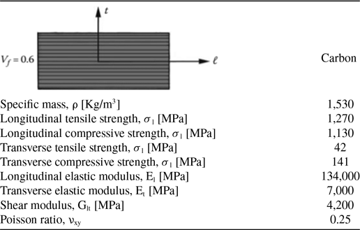


 Open access