





1. Introduction
Radio signals from pulsars undergo multipath propagation effects as they travel through the ionised interstellar medium (ISM) due to turbulence and electron density fluctuations. This leads to several observable effects, including scattering and scintillation – the modulation of the pulsar’s intensity across time and frequency. In the strong scattering regime – typical for pulsars observed at $\lesssim$
GHz frequencies – two scintillation time-scales arise: the diffractive (
$\lesssim$
GHz frequencies – two scintillation time-scales arise: the diffractive ( $\tau_\mathrm{dif}$
) and refractive (
$\tau_\mathrm{dif}$
) and refractive ( $\tau_\mathrm{ref}$
) interstellar scintillation (DISS and RISS, respectively). While the time-scales of RISS are typically long (
$\tau_\mathrm{ref}$
) interstellar scintillation (DISS and RISS, respectively). While the time-scales of RISS are typically long ( $\sim$
months), at
$\sim$
months), at $\sim$
1 GHz, the time-scales of DISS are on the order of minutes, with characteristic bandwidths of a few MHz. As a result, DISS is particularly useful for identifying pulsars in radio continuum surveys conducted at
$\sim$
1 GHz, the time-scales of DISS are on the order of minutes, with characteristic bandwidths of a few MHz. As a result, DISS is particularly useful for identifying pulsars in radio continuum surveys conducted at $\sim$
1 GHz with integration times ranging from one to several hours. Comprehensive reviews of interstellar scattering theory and related observations are provided by Rickett (Reference Rickett1990) and Narayan (Reference Narayan1992).
$\sim$
1 GHz with integration times ranging from one to several hours. Comprehensive reviews of interstellar scattering theory and related observations are provided by Rickett (Reference Rickett1990) and Narayan (Reference Narayan1992).
Previously, it has been proposed that DISS of radio pulsars can be used to distinguish them from other compact radio sources in radio continuum surveys. For example, Dai et al. (Reference Dai, Johnston, Bell, Coles, Hobbs, Ekers and Lenc2016) proposed to use the variance imaging technique to identify potential pulsar candidates in radio continuum observations by leveraging their DISS-induced flux density variability in time- and frequency-resolved radio images. The sensitivity of variance imaging depends critically on matching the temporal and spectral resolution of resolved images to the scintillation timescales and bandwidths of pulsars, respectively. If the time and frequency resolution are too low, DISS is smeared out; if too fine, background noise dominates the variance due to increased noise level in the subintegrations and channels. By optimising the number of subintegrations and channels, variance imaging provides a promising complement to traditional pulsar searches, enhancing the discovery potential in large-scale radio continuum surveys (Dai, Johnston, & Hobbs Reference Dai, Johnston and Hobbs2017). More recently, Salal, Tendulkar, & Marthi (Reference Salal, Tendulkar and Marthi2024) demonstrated a technique by stacking phased visibilities to form dynamic spectra and measuring their scintillation parameters using the upgraded Giant Metrewave Radio Telescope (uGMRT).
One of such deep all-sky survey is Evolutionary Map of the Universe (EMU; Hopkins et al. Reference Hopkins2025), which is being conducted by the Australian Square Kilometre Array Pathfinder (ASKAP) telescope. The capability of finding new pulsars using ASKAP’s image-based pulsar searches has been readily demonstrated by the discovery of pulsars originally identified as highly polarised radio sources (Kaplan et al. Reference Kaplan2019; Wang et al. Reference Wang2024, Reference Wang2025), pulsars associated with SNRs and pulsar wind nebulae (PWNe) (e.g. Ahmad et al. Reference Ahmad2025; Lazarević et al. Reference Lazarević2024), and highly scattered pulsars (e.g. Wang et al. Reference Wang2024; Lower et al. Reference Lower, Dai, Johnston and Barr2024; Sengar et al. Reference Sengar2026). Variance imaging with EMU will be more sensitive than current pulsar surveys at high Galactic latitudes in the Southern hemisphere and is expected to discover $\sim\!40$
new millisecond pulsars (MSPs) and
$\sim\!40$
new millisecond pulsars (MSPs) and $\sim\!30$
new normal pulsars (see Dai et al. Reference Dai, Johnston, Bell, Coles, Hobbs, Ekers and Lenc2016; Dai et al. Reference Dai, Johnston and Hobbs2017, and references therein). Image-based pulsar searches have also used spectral signature targeting steep-spectrum sources, polarisation, and variability in time using the Murchison Widefield Array (MWA) and MeerKAT continuum surveys (e.g. Frail et al. Reference Frail2018; Heywood Reference Heywood2023; Frail et al. Reference Frail2024; Sett et al. Reference Sett, Sokolowski, Lenc and Bhat2024; Mantovanini et al. Reference Mantovanini, Hurley-Walker, Anderson, Ross, Duchesne and Galvin2025).
$\sim\!30$
new normal pulsars (see Dai et al. Reference Dai, Johnston, Bell, Coles, Hobbs, Ekers and Lenc2016; Dai et al. Reference Dai, Johnston and Hobbs2017, and references therein). Image-based pulsar searches have also used spectral signature targeting steep-spectrum sources, polarisation, and variability in time using the Murchison Widefield Array (MWA) and MeerKAT continuum surveys (e.g. Frail et al. Reference Frail2018; Heywood Reference Heywood2023; Frail et al. Reference Frail2024; Sett et al. Reference Sett, Sokolowski, Lenc and Bhat2024; Mantovanini et al. Reference Mantovanini, Hurley-Walker, Anderson, Ross, Duchesne and Galvin2025).
The ASKAP telescope is also conducting the Variables and Slow Transients survey specifically to search for radio transients and variable sources on minute timescales (VAST, Murphy et al. Reference Murphy2013; Murphy et al. Reference Murphy2021; An et al. Reference An, Lao, Xu, Lu, Wang, Murphy, Kaplan and Guo2023). Variability studies on the first EMU Pilot survey show that the full EMU survey has great potential to identify such transients and variable sources (Wang et al. Reference Wang2023). More recently, several ultra-long period (ULP) sources (Hurley-Walker et al. Reference Hurley-Walker2022; Hurley-Walker et al. Reference Hurley-Walker2023), with periods of several minutes and repeating bursts of coherent radio emission, have also been reported with ASKAP (e.g. Caleb et al. Reference Caleb2024; Dobie et al. Reference Dobie2024; Lee et al. Reference Lee2025; Anumarlapudi et al. Reference Anumarlapudi2025). It is expected to discover more in the full EMU survey.
In this paper, we present a first pilot survey of pulsars using variance imaging with the EMU datasets. The primary aim of this work is to assess the feasibility and scientific potential of variance imaging with EMU. We focus on high Galactic latitude regions, where radio pulsars typically have lower dispersion measures (DMs), leading to broader scintillation bandwidths and longer scintillation timescales. As demonstrated by Dai et al. (Reference Dai, Johnston, Bell, Coles, Hobbs, Ekers and Lenc2016), the sensitivity of variance imaging is maximised when the time and frequency resolution match the pulsar’s scintillation properties. For low-DM pulsars, this allows us to adopt relatively coarse time and frequency resolutions and fix them at nominal values (see Section 3.1.2 for details) without a significant loss of sensitivity. In addition, high Galactic latitude regions are characterised by lower sky temperatures and reduced source confusion, owing to the relative absence of extended radio emission. This further simplifies the morphological complexity of the variance images. However, as discussed in Section 5, a blind search spanning a wide range of DMs would require variance images generated at multiple time and frequency resolutions, which would be computationally more expensive.
The organisation of this paper is as follows: in Section 2, we describe ASKAP and EMU surveys and Murriyang, the Parkes radio telescope’s observations and data analysis, followed by the description of variance imaging and source detection pipeline in Section 3. In Section 4, we present our results, including the discovery of three new pulsars, summarise the properties of known test pulsars and new candidates. In Section 5, we conclude and discuss the false alarms and potential problems, future improvements in the variance imaging pipeline, and application of this approach on future and ongoing radio continuum surveys, including the Galactic plane.
2. Observations
2.1. ASKAP observations
ASKAP is a radio interferometer consisting of 36 dishes, each with 12 m diameter, located at Inyarrimanha Ilgari Bundara, CSIRO’s Murchison Radio-astronomy Observatory, Western Australia (Hotan et al. Reference Hotan2021). Each dish is equipped with a phased array feed, which forms 36 dual polarisation beams on the sky, providing ASKAP with a wide field of view of $\sim$
30 square degrees. The EMU survey aims to make deep radio continuum maps covering the whole southern sky (
$\sim$
30 square degrees. The EMU survey aims to make deep radio continuum maps covering the whole southern sky ( $-90^{\circ}\leq DEC \leq +10^{\circ}$
) (Hopkins et al. Reference Hopkins2025). The survey is being conducted at a central frequency of 943.5 MHz with a bandwidth of 288 MHz. The total integration time for a typical observation is 10 h, reaching a sensitivity of 20–30
$-90^{\circ}\leq DEC \leq +10^{\circ}$
) (Hopkins et al. Reference Hopkins2025). The survey is being conducted at a central frequency of 943.5 MHz with a bandwidth of 288 MHz. The total integration time for a typical observation is 10 h, reaching a sensitivity of 20–30 $\unicode{x03BC}$
Jy beam
$\unicode{x03BC}$
Jy beam $^{-1}$
. Visibilities are recorded to capture full-Stokes information in 10 s integrations across 1 MHz-wide channels.
$^{-1}$
. Visibilities are recorded to capture full-Stokes information in 10 s integrations across 1 MHz-wide channels.
The data processing was done with the ASKAPsoft package (Guzman et al. Reference Guzman2019), including procedures such as calibration, flagging, and image generation. For each observation with a unique schedule block ID (SBID), ASKAPsoft produces calibrated visibilities for 36 individual primary beams in the form of complex values as a function of time, frequency, baseline, and correlations and stored in a measurement set (MS) format. A corresponding full-Stokes radio continuum image for the entire field of view is also produced. Total intensity catalogues and noise maps are generated with Selavy (Whiting & Humphreys Reference Whiting and Humphreys2012), and data are automatically uploaded to the CSIRO ASKAP Science Data Archive (CASDAFootnote a ) and made publicly available after completing scientific validation.
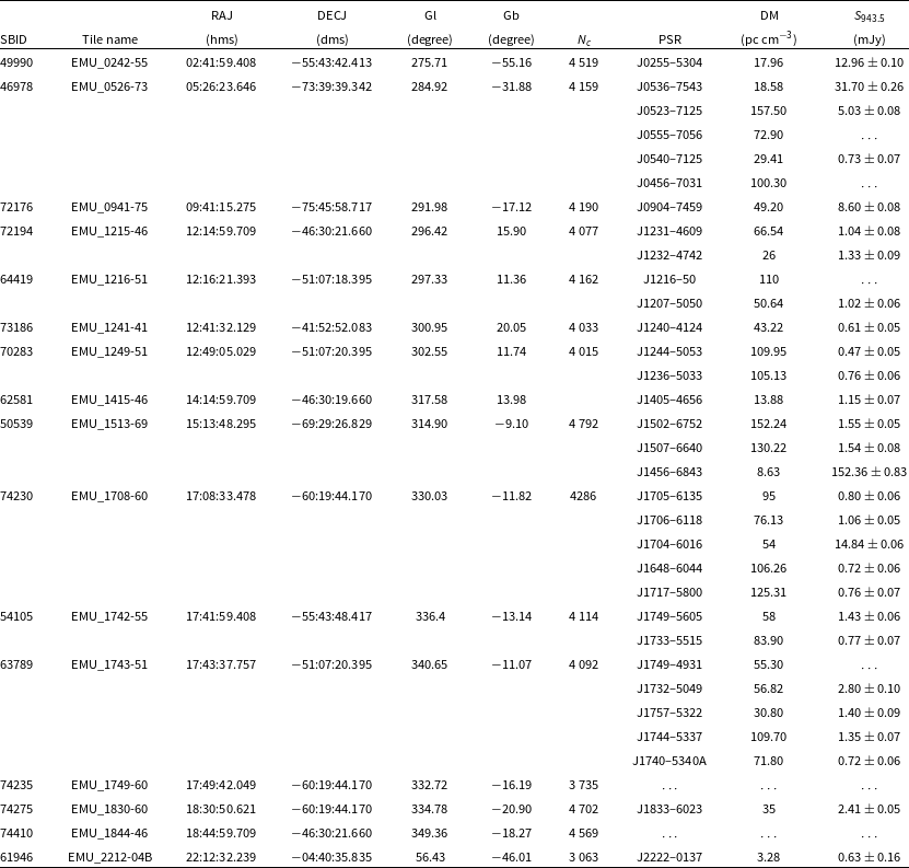
As explained earlier, this paper focuses on high Galactic latitude regions. Sixteen EMU tiles at high Galactic latitudes (Table 1) were downloaded from CASDA and used for analysis. These contain 32 known pulsars within the total field of view, and we successfully detected 28 of them as continuum sources within a DM range of $\sim$
3–157 pc cm
$\sim$
3–157 pc cm $^{-3}$
. Of the four pulsars not detected by EMU, three have measured flux densities at 1.4 GHz. All three pulsars (J0555–7056, J0456–7031 and J1749–4931) have flux densities
$^{-3}$
. Of the four pulsars not detected by EMU, three have measured flux densities at 1.4 GHz. All three pulsars (J0555–7056, J0456–7031 and J1749–4931) have flux densities $\lesssim$ $0.1$
mJy. Their flux densities are below the
$0.1$
mJy. Their flux densities are below the $\sim5\sigma$
sensitivity threshold of their corresponding EMU continuum images, explaining their non-detection. PSR J1216–50 is a rotating radio transient, and only single pulses have been detected (Burke-Spolaor et al. Reference Burke-Spolaor2011).
$\sim5\sigma$
sensitivity threshold of their corresponding EMU continuum images, explaining their non-detection. PSR J1216–50 is a rotating radio transient, and only single pulses have been detected (Burke-Spolaor et al. Reference Burke-Spolaor2011).
Sixteen high Galactic latitude EMU tiles are listed in this table. Columns include schedule block ID (SBID), EMU tile name, central coordinates (RAJ $\&$
DECJ), Galactic longitude and latitude (Gl
$\&$
DECJ), Galactic longitude and latitude (Gl $\&$
Gb), number of compact sources in the tiles (
$\&$
Gb), number of compact sources in the tiles ( $N_{c}$
), known pulsars along with respective DMs taken from ATNF Pulsar Catalogue (Manchester et al. Reference Manchester, Hobbs, Teoh and Hobbs2005), and pulsar flux densities at 943.5 MHz from EMU. Each tile spans a duration of 10 h, except the SB 61946, with a total observing duration of five hours. Tiles without a listed pulsar contain no known pulsars in their field of view.
$N_{c}$
), known pulsars along with respective DMs taken from ATNF Pulsar Catalogue (Manchester et al. Reference Manchester, Hobbs, Teoh and Hobbs2005), and pulsar flux densities at 943.5 MHz from EMU. Each tile spans a duration of 10 h, except the SB 61946, with a total observing duration of five hours. Tiles without a listed pulsar contain no known pulsars in their field of view.

2.2. Murriyang observations
We conducted follow-up observations of pulsar candidates identified in variance images using Murriyang’s Ultra-Wideband Low (UWL) receiver in conjunction with the Medusa backend (Hobbs et al. Reference Hobbs2020). The total integration time ranged from 0.5 to 4 h and only the total intensity was recorded. Data were recorded in pulsar search mode with 2-bit sampling every 64 $\unicode{x03BC}$
s within 0.125 MHz wide frequency channels, totalling 26 624 channels covering 704–4032 MHz. Since pulsars detected in variance images show strong scintillation, we searched for their periodicity over a wide bandwidth from 1344 to 3264 MHz. This frequency range was chosen to avoid strong radio frequency interference (RFI) at lower frequencies and maximise our chance of detecting scintillating pulsars. The periodicity search was performed using a pulsar searching pipeline based on the PRESTO software package (Ransom Reference Ransom2011). Periodic signals were searched within a DM range of 0–500 pc cm
$\unicode{x03BC}$
s within 0.125 MHz wide frequency channels, totalling 26 624 channels covering 704–4032 MHz. Since pulsars detected in variance images show strong scintillation, we searched for their periodicity over a wide bandwidth from 1344 to 3264 MHz. This frequency range was chosen to avoid strong radio frequency interference (RFI) at lower frequencies and maximise our chance of detecting scintillating pulsars. The periodicity search was performed using a pulsar searching pipeline based on the PRESTO software package (Ransom Reference Ransom2011). Periodic signals were searched within a DM range of 0–500 pc cm $^{-3}$
in the Fourier domain. Candidates with a signal-to-noise ratio threshold of
$^{-3}$
in the Fourier domain. Candidates with a signal-to-noise ratio threshold of $\gt$
8 were folded and inspected visually.
$\gt$
8 were folded and inspected visually.
Follow-up observations of confirmed pulsar discoveries were carried out with the coherently dedispersed search mode using the UWL system. The total intensity was recorded with 2-bit sampling every 64 $\unicode{x03BC}$
s and 1 MHz frequency resolution, totalling 3 328 channels covering 704–4 032 MHz. Search mode data were folded using the DSPSR software package (van Straten & Bailes Reference van Straten and Bailes2011) with a sub-integration length of 30 s. Folded pulse profiles were then processed and calibrated with the PSRCHIVE software package (Hotan, van Straten, & Manchester Reference Hotan, van Straten and Manchester2004). Each observation was visually examined using the pazi program to remove RFI and then averaged in time to form an averaged pulse profile. The pulse time of arrivals (ToAs) was measured for each observation using the pat routine of PSRCHIVE. Timing analysis was carried out using the TEMPO2 software package (Hobbs, Edwards, & Manchester Reference Hobbs, Edwards and Manchester2006).
$\unicode{x03BC}$
s and 1 MHz frequency resolution, totalling 3 328 channels covering 704–4 032 MHz. Search mode data were folded using the DSPSR software package (van Straten & Bailes Reference van Straten and Bailes2011) with a sub-integration length of 30 s. Folded pulse profiles were then processed and calibrated with the PSRCHIVE software package (Hotan, van Straten, & Manchester Reference Hotan, van Straten and Manchester2004). Each observation was visually examined using the pazi program to remove RFI and then averaged in time to form an averaged pulse profile. The pulse time of arrivals (ToAs) was measured for each observation using the pat routine of PSRCHIVE. Timing analysis was carried out using the TEMPO2 software package (Hobbs, Edwards, & Manchester Reference Hobbs, Edwards and Manchester2006).
3. Variance imaging and source detection
3.1. Imaging pipeline
Our data processing pipeline involves several steps to produce final products (dynamic spectra) from calibrated visibilities. All data processing has been done on OzSTARFootnote b computing facility with Common Astronomy Software Applications (CASA; CASA Team et al. Reference Team2022) package in combination with Python scripts. The details of each tile are given in Table 1. We downloaded the visibility data comprising 576 MS (36 beams per tile) and selavy catalogues from CASDA to the Ozstar for further processing. The data downloading process takes about 3 h. We processed each beam independently, and the steps of our dedicated processing are described further.
3.1.1. Pre-processing of measurement set
The processing of calibrated visibility data using the CASA package requires the MS to be corrected for beam phase centre and flux density scale. ASKAP visibilities, processed with the ASKAPsoft pipeline, are stored on a per-beam basis. However, by default, the phase direction of each per-beam MS in the FIELD table is set to the telescope pointing direction, while the offsets from the centers of the 36 individual beams are stored in the FEED table. The non-ASKAPsoft imagers such as CASA do not account for the FEED table, and the phase direction in the FIELD table requires a prior correction by applying the appropriate beam offsets from the FEED table. ASKAPsoft also defines the Stokes parameters based on the total flux density of orthogonal correlations (e.g. $I = XX + YY$
), whereas CASA uses Stokes definitions based on the average flux density (e.g.
$I = XX + YY$
), whereas CASA uses Stokes definitions based on the average flux density (e.g. $I = (XX + YY)/2$
). Therefore, a beam offset and flux density scale correction was applied to each MS prior to CASA imaging using the command line script dstools-askap-preprocess of DSTOOLS (Pritchard Reference Pritchard2025). The pre-processing step takes a few minutes for a 10 h observation.
$I = (XX + YY)/2$
). Therefore, a beam offset and flux density scale correction was applied to each MS prior to CASA imaging using the command line script dstools-askap-preprocess of DSTOOLS (Pritchard Reference Pritchard2025). The pre-processing step takes a few minutes for a 10 h observation.
3.1.2. Image creation
The EMU tiles selected for this work are located at relatively high Galactic latitudes ( $|\mathrm{Gb}| \gt 9^{\circ}$
). As shown in Table 1, among the 28 known pulsars detected within these EMU tiles, eight have DMs below
$|\mathrm{Gb}| \gt 9^{\circ}$
). As shown in Table 1, among the 28 known pulsars detected within these EMU tiles, eight have DMs below $\sim$
30 pc cm
$\sim$
30 pc cm $^{-3}$
, indicating the presence of a low-DM pulsar population in these regions of the sky. Our pilot survey is targeted at these low-DM pulsars. To determine the frequency and time resolution required for variance imaging, we first calculated the expected scattering time (
$^{-3}$
, indicating the presence of a low-DM pulsar population in these regions of the sky. Our pilot survey is targeted at these low-DM pulsars. To determine the frequency and time resolution required for variance imaging, we first calculated the expected scattering time ( $\tau_{s}$
) using the relation obtained by Krishnakumar et al. (Reference Krishnakumar, Mitra, Naidu, Joshi and Manoharan2015) and scaled to 1 GHz assuming
$\tau_{s}$
) using the relation obtained by Krishnakumar et al. (Reference Krishnakumar, Mitra, Naidu, Joshi and Manoharan2015) and scaled to 1 GHz assuming $\tau_{s}$ $\approx$ $\nu^\mathrm{-4}$
dependence:
$\nu^\mathrm{-4}$
dependence:
 \begin{equation} \tau_{s,1\,\textrm{GHz}} (\unicode{x03BC}\,\mathrm{s}) = 4.1 \times 10^{-5} DM^{2.2} (1 + 0.00194 DM^{2}).\end{equation}
Assuming a homogeneous medium with a Kolmogorov spectrum (Cordes & Rickett Reference Cordes and Rickett1998), the scintillation bandwidth ( $\nu_\mathrm{diss}$
) can be obtained by,
$\nu_\mathrm{diss}$
) can be obtained by,
 \begin{equation} 2\pi\nu_\mathrm{diss}\tau_{s}=C_{1},\end{equation}
where $C_{1}=1.16$
for a uniform medium with a Kolmogorov wavenumber spectrum. The scintillation time-scale,
$C_{1}=1.16$
for a uniform medium with a Kolmogorov wavenumber spectrum. The scintillation time-scale, $\tau_\mathrm{diss}$
, can be estimated as (Johnston et al. Reference Johnston, Nicastro and Koribalski1998),
$\tau_\mathrm{diss}$
, can be estimated as (Johnston et al. Reference Johnston, Nicastro and Koribalski1998),
 \begin{equation} \tau_\mathrm{diss} = \frac{3.85 \times 10^{4} \sqrt{D \nu_\mathrm{diss}}}{\nu V} ,\end{equation}
where $\nu$
is the observing frequency in GHz, D is the distance to pulsar in kpc, and V is the speed of the interstellar diffraction pattern relative to the Earth in units of km s
$\nu$
is the observing frequency in GHz, D is the distance to pulsar in kpc, and V is the speed of the interstellar diffraction pattern relative to the Earth in units of km s $^{-1}$
, dominated by the pulsar transverse velocity.
$^{-1}$
, dominated by the pulsar transverse velocity.
For DMs in the range 5–30 pc cm $^{-3}$
, the expected scintillation bandwidth is approximately 10–50 MHz. Assuming a nominal transverse velocity of 100 km s
$^{-3}$
, the expected scintillation bandwidth is approximately 10–50 MHz. Assuming a nominal transverse velocity of 100 km s $^{-1}$
and pulsar distance of 1 kpc, the corresponding scintillation timescale is 7–60 min. Accordingly, for each beam we adopt a frequency resolution of 24 MHz and a time resolution of 20 min, resulting in 360 images for a typical 10 h observation. Although these fixed time and frequency resolutions are not optimal for all possible DMs, they are sufficient for the purposes of this pilot survey.
$^{-1}$
and pulsar distance of 1 kpc, the corresponding scintillation timescale is 7–60 min. Accordingly, for each beam we adopt a frequency resolution of 24 MHz and a time resolution of 20 min, resulting in 360 images for a typical 10 h observation. Although these fixed time and frequency resolutions are not optimal for all possible DMs, they are sufficient for the purposes of this pilot survey.
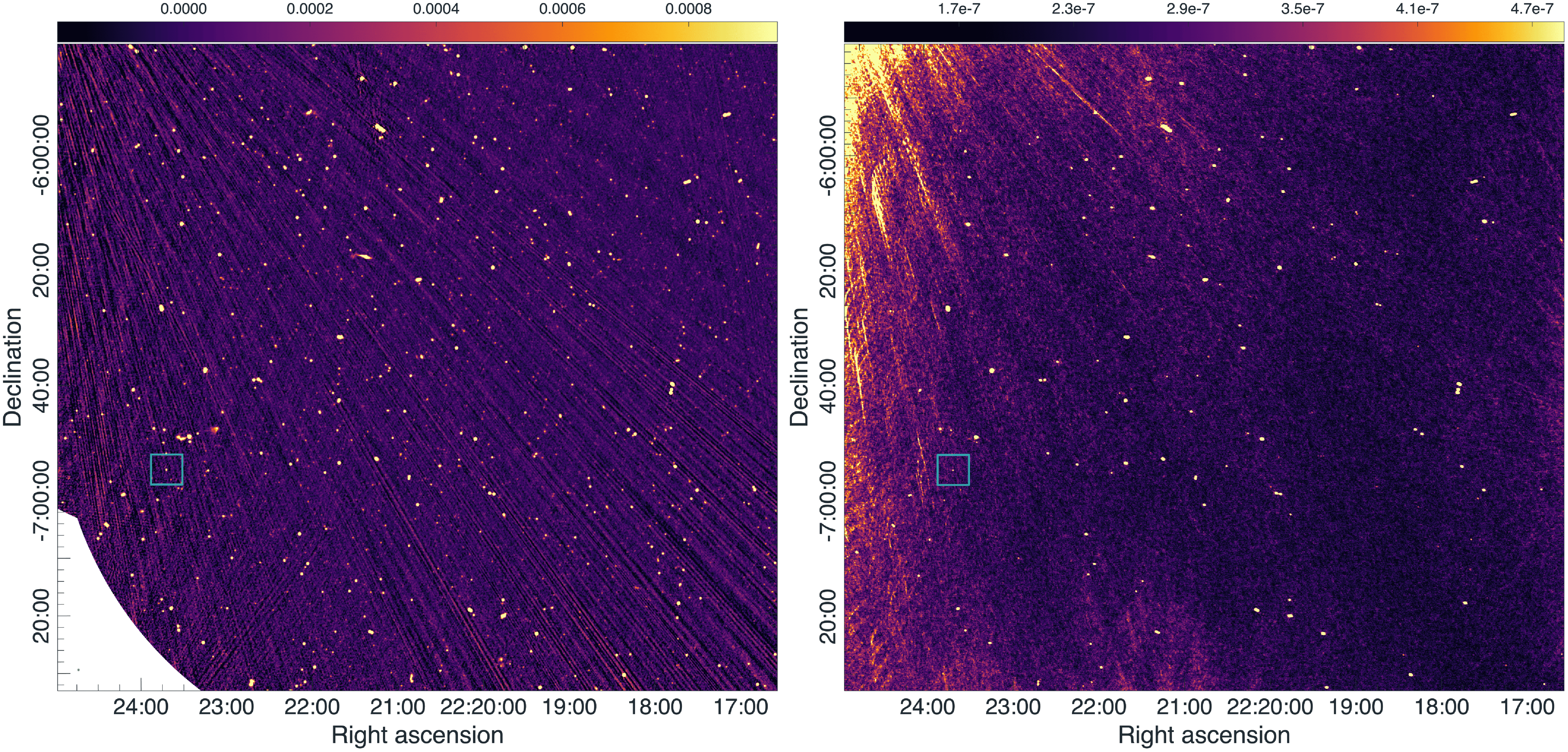
Left: A portion of the EMU radio-continuum image of the tile ‘EMU_2212-04B’ (SB 61946) at 943.5 MHz from CASDA. The field of view is $2\times 2$
deg
$2\times 2$
deg $^{2}$
. The white region at the bottom-left corner lies outside the FWHM for the primary beam, which is approximately
$^{2}$
. The white region at the bottom-left corner lies outside the FWHM for the primary beam, which is approximately $1.5^\circ$
. The beam size of the radio image is 15 arcsec
$1.5^\circ$
. The beam size of the radio image is 15 arcsec $\times$
15 arcsec and shown at the bottom left corner. The colour bar is in units of Jy beam
$\times$
15 arcsec and shown at the bottom left corner. The colour bar is in units of Jy beam $^{-1}$
. Right: The corresponding variance image (beam 05) containing the new pulsar J2223–0654 in a square box. The region of enhanced variance at the top left corner and towards right end of the image is due to the sidelobes of out-of-beam bright sources.
$^{-1}$
. Right: The corresponding variance image (beam 05) containing the new pulsar J2223–0654 in a square box. The region of enhanced variance at the top left corner and towards right end of the image is due to the sidelobes of out-of-beam bright sources.

To clean and produce snapshot images from corrected visibility data, we employed the tclean functionality of CASA using a default version of CLEAN deconvolver (Högbom Reference Högbom1974). We did not produce and subtract a sky model from the calibrated visibilities, nor did we include higher-order spectral terms in the imaging. We performed cleaning with 10 000 iterations using Briggs weighting with robustness of 0.5 to obtain an optimal balance between sensitivity and resolution (Briggs Reference Briggs1995). The deconvolution was performed using a purely threshold-based approach without applying any CLEAN masks. We adopted a CLEAN threshold of 1 mJy, which is approximately 2–3 $\sigma$
of the theoretical snapshot rms of
$\sigma$
of the theoretical snapshot rms of $\sim 0.40$
mJy for selected time and frequency resolution, ensuring adequate deconvolution of real sources while avoid cleaning into the noise. Baselines shorter than 100 m were flagged following previous ASKAP imaging practice (e.g. An et al. Reference An, Lao, Xu, Lu, Wang, Murphy, Kaplan and Guo2023; Duchesne et al. Reference Duchesne2025; Lee et al. Reference Lee2026). These short baselines are primarily sensitive to large-scale diffuse emission and are not relevant to our science goal of identifying compact, variable sources through variance imaging. Excluding short baselines suppresses diffuse extended radio emission, improves image quality with reduced rms noise, and accelerates the generation of snapshot images with optimised computational cost. The rms noise is reduced by
$\sim 0.40$
mJy for selected time and frequency resolution, ensuring adequate deconvolution of real sources while avoid cleaning into the noise. Baselines shorter than 100 m were flagged following previous ASKAP imaging practice (e.g. An et al. Reference An, Lao, Xu, Lu, Wang, Murphy, Kaplan and Guo2023; Duchesne et al. Reference Duchesne2025; Lee et al. Reference Lee2026). These short baselines are primarily sensitive to large-scale diffuse emission and are not relevant to our science goal of identifying compact, variable sources through variance imaging. Excluding short baselines suppresses diffuse extended radio emission, improves image quality with reduced rms noise, and accelerates the generation of snapshot images with optimised computational cost. The rms noise is reduced by $\sim$
15% after excluding the shorter baselines. The adopted imaging strategy was found to be sufficient to deliver clean residuals for the snapshot imaging performed in this work. We chose an image cell size of 2 arcsec, an image size of
$\sim$
15% after excluding the shorter baselines. The adopted imaging strategy was found to be sufficient to deliver clean residuals for the snapshot imaging performed in this work. We chose an image cell size of 2 arcsec, an image size of $4\,000\times 4\,000$
pixels to include as many of the neighbouring sources to reduce the sidelobes effect, and a widefield gridding option. A
$4\,000\times 4\,000$
pixels to include as many of the neighbouring sources to reduce the sidelobes effect, and a widefield gridding option. A $4\,000\times 4\,000$
pixel image corresponds to a square field of view (FoV) of approximately 2.2
$4\,000\times 4\,000$
pixel image corresponds to a square field of view (FoV) of approximately 2.2 $^{\circ}$
, which is about 1.5 times the full width half maximum (FWHM) of primary beam at 943.5 MHz.
$^{\circ}$
, which is about 1.5 times the full width half maximum (FWHM) of primary beam at 943.5 MHz.
In total, we generated $\sim$
200,880 images for all 576 MS. The runtime for each tclean job was approximately 0.5 h. Due to a limit on maximum number of concurrent jobs on Oz STAR, up to five MS were processed simultaneously. Under these constraints, the snapshot imaging was completed in approximately 58 h. The typical residual rms of the resulting images is between 400 and 600
$\sim$
200,880 images for all 576 MS. The runtime for each tclean job was approximately 0.5 h. Due to a limit on maximum number of concurrent jobs on Oz STAR, up to five MS were processed simultaneously. Under these constraints, the snapshot imaging was completed in approximately 58 h. The typical residual rms of the resulting images is between 400 and 600 $\unicode{x03BC}$
Jy beam
$\unicode{x03BC}$
Jy beam $^{-1}$
.
$^{-1}$
.
3.1.3. Variance image creation
Variance images are generated by calculating the variance of radio flux densities for each image pixel across time and frequency. This step takes approximately 20 min per EMU tile. No weighting was applied in the construction of the variance maps from the snapshot images, as the large flux density fluctuations caused by diffractive scintillation are intrinsically random in both time and frequency. An example variance image (beam 05 of SB61946) is presented in Figure 1 (right), where the newly identified pulsar J2223–0654 (see Section 4.2) is marked with a square box. The pronounced artefacts and elevated noise in the upper-left region arise from contamination by a bright ( $\sim$
10 Jy) source located
$\sim$
10 Jy) source located $2^\circ$
from the beam centre, outside the primary beam. The streak-like artefacts from the source is also visible in the corresponding EMU continuum image from CASDA (left). Artefacts and locally enhanced noise can also appear on small angular scales, most commonly in the vicinity of bright or extended sources. These features arise from a combination of residual time- and frequency-dependent PSF variations, direction-dependent calibration errors, and sidelobes associated with imperfect deconvolution. However, the variability introduced by such artefacts is significantly weaker than that produced by scintillation and can be efficiently excluded using the selection criteria described below.
$2^\circ$
from the beam centre, outside the primary beam. The streak-like artefacts from the source is also visible in the corresponding EMU continuum image from CASDA (left). Artefacts and locally enhanced noise can also appear on small angular scales, most commonly in the vicinity of bright or extended sources. These features arise from a combination of residual time- and frequency-dependent PSF variations, direction-dependent calibration errors, and sidelobes associated with imperfect deconvolution. However, the variability introduced by such artefacts is significantly weaker than that produced by scintillation and can be efficiently excluded using the selection criteria described below.
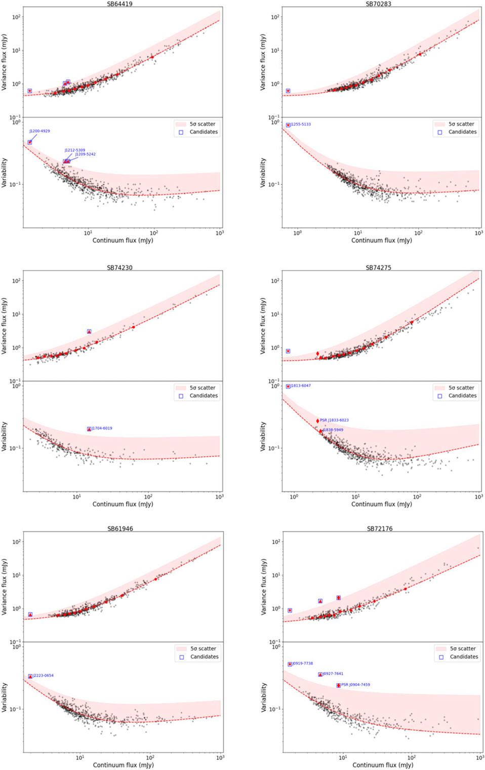
Top panels: Variance flux density versus continuum flux density for sources detected in the variance images of six tiles in which pulsar and radio star candidates are identified. The red solid circles indicate the median variance flux densities in ten equal-population continuum flux bins. The red dashed lines show the power-law fits to these median values. Bottom panels: Variability (R) versus continuum flux density for the same sources, where R is defined as the ratio of variance flux density ( $S_{v}$
) to continuum flux density (
$S_{v}$
) to continuum flux density ( $S_\mathrm{ 943.5}$
). The red dashed lines represent the expected flux-dependent variability derived from the power-law fits shown in the top panels. Blue squares highlight highly variable sources that exceed the
$S_\mathrm{ 943.5}$
). The red dashed lines represent the expected flux-dependent variability derived from the power-law fits shown in the top panels. Blue squares highlight highly variable sources that exceed the $5\sigma$
scatter (shaded region) relative to the fit. Red symbols denote known pulsars (diamonds), pulsar candidates (triangles), and radio stars (asterisks). The radio stars exhibit relatively higher variability despite being the faintest (
$5\sigma$
scatter (shaded region) relative to the fit. Red symbols denote known pulsars (diamonds), pulsar candidates (triangles), and radio stars (asterisks). The radio stars exhibit relatively higher variability despite being the faintest ( $S_{943.5} \leq$
1 mJy) in our sample, consistent with potential radio flares.
$S_{943.5} \leq$
1 mJy) in our sample, consistent with potential radio flares.

3.2. Candidate selection
To identify pulsar candidates in variance images, we first select compact radio sources in the Selavy catalogues, which are produced by the EMU pipeline. We employ a compactness criterion defined as the ratio of the integrated flux density ( $S_\mathrm{int}$
) to the peak flux density (
$S_\mathrm{int}$
) to the peak flux density ( $S_{p}$
) of the sources in the EMU continuum image. Specifically, sources with compactness
$S_{p}$
) of the sources in the EMU continuum image. Specifically, sources with compactness $\gt$
1.5 and/or with multiple Selavy components are regarded as extended and excluded from our further analysis. In addition, weak sources with
$\gt$
1.5 and/or with multiple Selavy components are regarded as extended and excluded from our further analysis. In addition, weak sources with $S_\mathrm{int}/\sigma_\mathrm{rms} \leq 5$
and the sources with flux density uncertainties exceeding 10% are also excluded. For each EMU tile, the number of compact sources selected by these criteria is given in Table 1. This compactness criterion may exclude genuine scintillating pulsars that are embedded in complex structures such as pulsar wind nebulae (PWNe) or supernova remnants (SNRs). However, these young and energetic pulsars are predominantly found in the Galactic plane (e.g. Kargaltsev et al. Reference Kargaltsev, Pavlov, Klingler and Rangelov2017; Green Reference Green2025), and are therefore not primary targets of this high–Galactic-latitude pilot survey.
$S_\mathrm{int}/\sigma_\mathrm{rms} \leq 5$
and the sources with flux density uncertainties exceeding 10% are also excluded. For each EMU tile, the number of compact sources selected by these criteria is given in Table 1. This compactness criterion may exclude genuine scintillating pulsars that are embedded in complex structures such as pulsar wind nebulae (PWNe) or supernova remnants (SNRs). However, these young and energetic pulsars are predominantly found in the Galactic plane (e.g. Kargaltsev et al. Reference Kargaltsev, Pavlov, Klingler and Rangelov2017; Green Reference Green2025), and are therefore not primary targets of this high–Galactic-latitude pilot survey.
The Selavy catalogues generated by the EMU pipeline exclude sources close to the edge of tiles. While the edges of tiles often show reduced sensitivity, we found that strong compact radio sources can be well detected in variance images. Therefore, to avoid missing potentially interesting variable sources in these regions, we manually inspected the variance images of the outermost beams using Cube Analysis and Rendering Tool for Astronomy (CARTA; Comrie et al. Reference Comrie2021). For compact sources that can be clearly detected in variance images, we measured their continuum flux density using CARTA and included them in our following analysis.
To identify high-confidence sources in the variance images, we fitted a two-dimensional Gaussian to the variance flux density at the position of each compact source selected from the Selavy catalogues. The full width at half maximum (FWHM) of each source was estimated as $B_\mathrm{source} = 2.355 \times r$
, where r is defined as
$B_\mathrm{source} = 2.355 \times r$
, where r is defined as $(\sigma_{x}\times\sigma_{y})^{1/2}$
, and
$(\sigma_{x}\times\sigma_{y})^{1/2}$
, and $\sigma_{x}$
and
$\sigma_{x}$
and $\sigma_{y}$
are the standard deviations along the x and y directions, respectively. For point-like continuum sources with flat spectra and no variability, the expected size of their counterparts in the variance images (
$\sigma_{y}$
are the standard deviations along the x and y directions, respectively. For point-like continuum sources with flat spectra and no variability, the expected size of their counterparts in the variance images ( $B_\mathrm{var}$
) can be approximated by the synthesised beam size of the lowest-frequency band used for variance imaging, since the snapshot images were not convolved to a common resolution. Although the shape of the synthesised beam is time dependent, its variation is small; we measured an average value of
$B_\mathrm{var}$
) can be approximated by the synthesised beam size of the lowest-frequency band used for variance imaging, since the snapshot images were not convolved to a common resolution. Although the shape of the synthesised beam is time dependent, its variation is small; we measured an average value of $B_\mathrm{var} \approx 20$
arcsec, corresponding to approximately 10 pixels, consistently across all 16 fields. We compared
$B_\mathrm{var} \approx 20$
arcsec, corresponding to approximately 10 pixels, consistently across all 16 fields. We compared $B_\mathrm{source}$
with
$B_\mathrm{source}$
with $B_\mathrm{var}$
, and rejected sources if
$B_\mathrm{var}$
, and rejected sources if $B_\mathrm{source}$
exceeded
$B_\mathrm{source}$
exceeded $B_\mathrm{var}$
or if their fitted positions were offset from the corresponding continuum source positions by more than
$B_\mathrm{var}$
or if their fitted positions were offset from the corresponding continuum source positions by more than $B_\mathrm{source}$
. This approach effectively removes sources in the variance images that are significantly affected by imaging artefacts (see Section 5 for further discussion). The variance flux densities (
$B_\mathrm{source}$
. This approach effectively removes sources in the variance images that are significantly affected by imaging artefacts (see Section 5 for further discussion). The variance flux densities ( $S_{v}$
) of the sources are then measured by integrating pixel values within a contour at 10% of the peak of the Gaussian distribution. The rms noise (
$S_{v}$
) of the sources are then measured by integrating pixel values within a contour at 10% of the peak of the Gaussian distribution. The rms noise ( $\sigma_{v}$
) of the background is measured within an annulus region
$\sigma_{v}$
) of the background is measured within an annulus region $3B_{\mathrm{source}}\lt r\lt 6B_{\mathrm{source}}$
centred at the source positions. Finally, we select sources with
$3B_{\mathrm{source}}\lt r\lt 6B_{\mathrm{source}}$
centred at the source positions. Finally, we select sources with $S_{v}/\sigma_{v}\geq5$
as reliable detections in the variance image.
$S_{v}/\sigma_{v}\geq5$
as reliable detections in the variance image.
Sources showing up in the variance image consist of potential pulsars, variable sources, steep-spectrum sources, and extremely bright sources. However, we expect scintillating pulsars to show the highest level of variability in variance images. In Figure 2, the top panel shows the variance flux density ( $S_{v}$
) as a function of continuum flux density (
$S_{v}$
) as a function of continuum flux density ( $S_{943.5}$
) for all sources detected in the variance image for an EMU tile. For sources exhibiting low levels of variability, brighter sources naturally display higher absolute variance than fainter ones, which explains the trend observed in Figure 2. To identify pulsar candidates, we sorted the sources by continuum flux density and divided them into ten equal-population bins. For each bin, we computed the median continuum and variance flux densities, shown as red solid circles in the upper panel of Figure 2. We then fitted a power law to these median values as a function of continuum flux density, plotted as the red dashed curve in the same panel. This method provides robust statistics within each bin, while naturally producing narrower bins at low flux densities, where sources are abundant, and wider bins at higher flux densities, where sources are sparse. The lower panel of Figure 2 presents the variability, R, defined as the ratio of variance flux density (
$S_{943.5}$
) for all sources detected in the variance image for an EMU tile. For sources exhibiting low levels of variability, brighter sources naturally display higher absolute variance than fainter ones, which explains the trend observed in Figure 2. To identify pulsar candidates, we sorted the sources by continuum flux density and divided them into ten equal-population bins. For each bin, we computed the median continuum and variance flux densities, shown as red solid circles in the upper panel of Figure 2. We then fitted a power law to these median values as a function of continuum flux density, plotted as the red dashed curve in the same panel. This method provides robust statistics within each bin, while naturally producing narrower bins at low flux densities, where sources are abundant, and wider bins at higher flux densities, where sources are sparse. The lower panel of Figure 2 presents the variability, R, defined as the ratio of variance flux density ( $S_{v}$
) to continuum flux density (
$S_{v}$
) to continuum flux density ( $S_\mathrm{943.5}$
). The red dashed curve indicates the expected variability, obtained by dividing the power-law fit from the upper panel by the continuum flux density. Sources deviating by more than +
$S_\mathrm{943.5}$
). The red dashed curve indicates the expected variability, obtained by dividing the power-law fit from the upper panel by the continuum flux density. Sources deviating by more than + $5\sigma$
from the best-fit curve were selected as candidates, with known pulsars and pulsar candidates highlighted by blue squares. The candidate selection criteria take about a few minutes per EMU tile.
$5\sigma$
from the best-fit curve were selected as candidates, with known pulsars and pulsar candidates highlighted by blue squares. The candidate selection criteria take about a few minutes per EMU tile.
In addition to applying the variability threshold, we generated circular polarisation cutout images for all sources detected in the variance maps. The circular polarisation leakage in ASKAP is typically less than 1%, increasing to $\sim$
2% toward the outer edges of the images (e.g. Pritchard et al. Reference Pritchard2021). Therefore, sources exhibiting significant circular polarisation (
$\sim$
2% toward the outer edges of the images (e.g. Pritchard et al. Reference Pritchard2021). Therefore, sources exhibiting significant circular polarisation ( $|V|/I \gt 5\%$
) were identified as pulsar candidates for follow-up observations. In total, 22 variable sources were detected in the whole survey area, including 10 known pulsars. Of the 22 candidates flagged, one was rejected in SB54105 upon manual inspection due to spurious morphology (e.g. extended or asymmetric structure) inconsistent with a point source. The low rejection rate indicates that the majority of the sources are adequately deconvolved and that the selection criteria effectively isolate genuine compact variable sources while filtering out most artefacts.
$|V|/I \gt 5\%$
) were identified as pulsar candidates for follow-up observations. In total, 22 variable sources were detected in the whole survey area, including 10 known pulsars. Of the 22 candidates flagged, one was rejected in SB54105 upon manual inspection due to spurious morphology (e.g. extended or asymmetric structure) inconsistent with a point source. The low rejection rate indicates that the majority of the sources are adequately deconvolved and that the selection criteria effectively isolate genuine compact variable sources while filtering out most artefacts.
3.3. Candidate verification
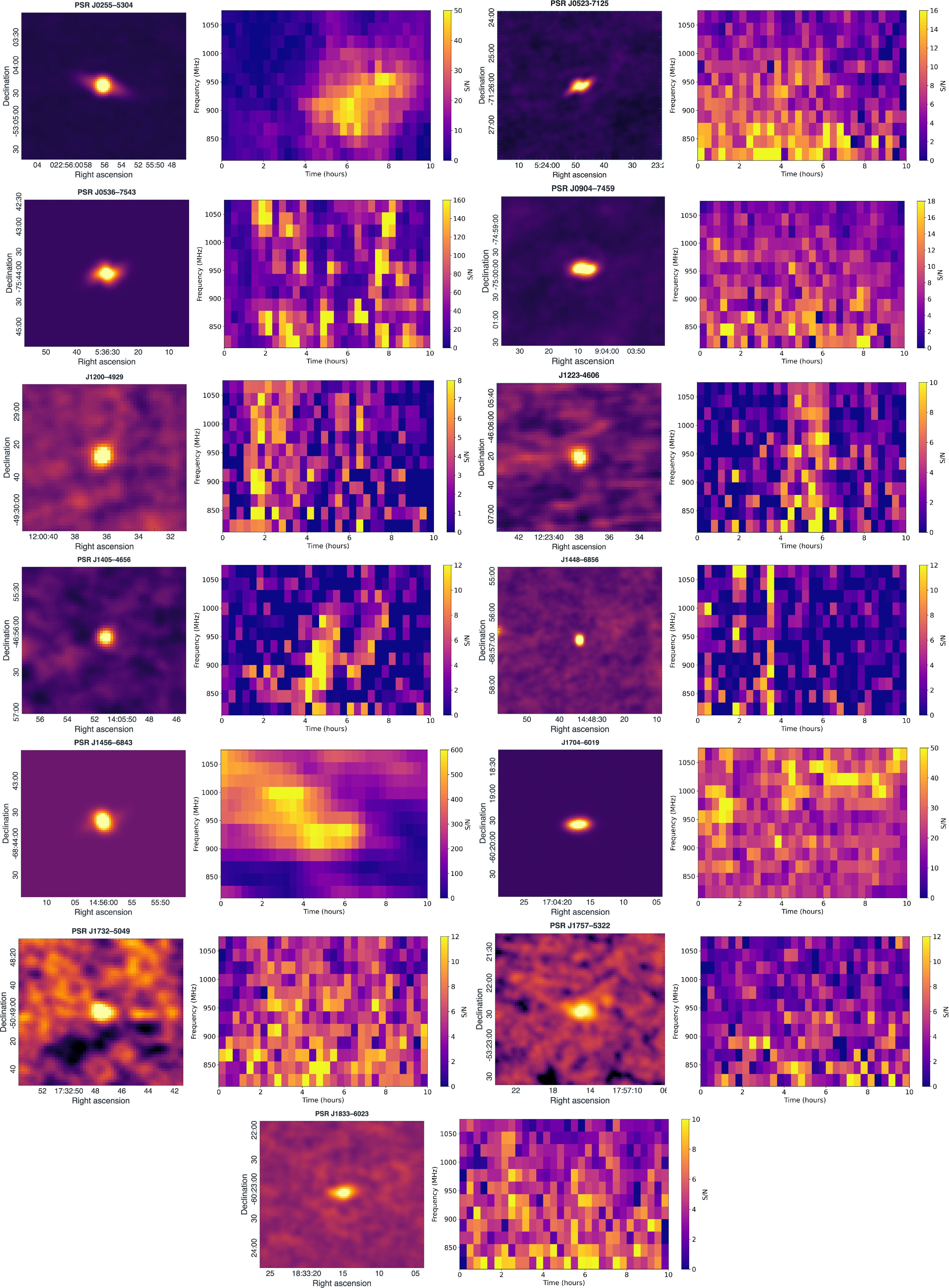
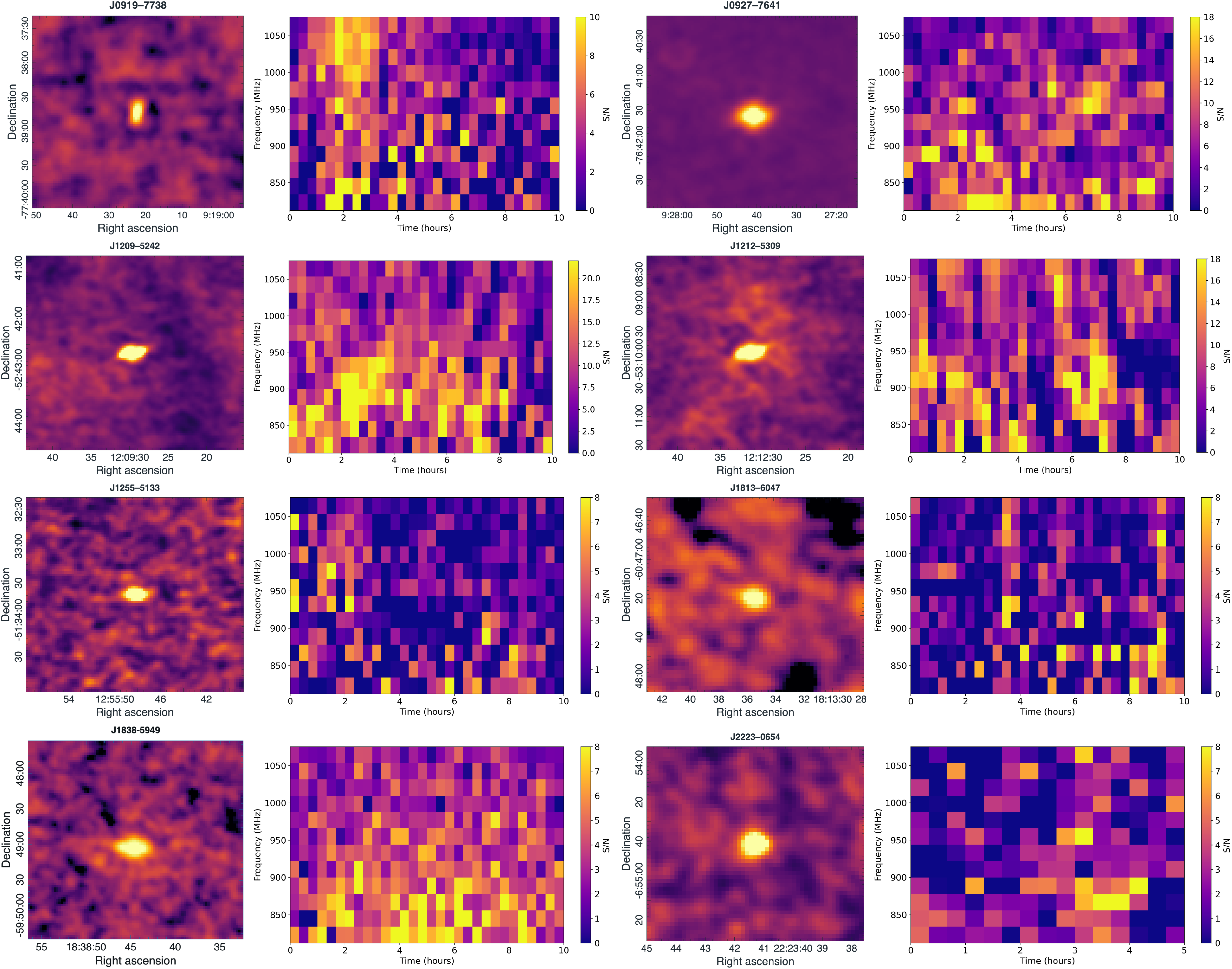
The candidate selection criteria described in Section 3.2 are shown to be efficient. Several known pulsars and radio stars stand out as outliers showing the highest level of variability. In each of our EMU tiles, we are able to reduce the number of candidates to fewer than four from a large number of compact sources (see Table 1). To verify pulsar candidates, we produced a dynamic spectrum for each of these candidates by measuring the signal-to-noise ratio (S/N) of the source in each fine time and frequency resolution image. Examples of dynamic spectra for pulsars and pulsar candidates are shown in Figures 3 and 4, respectively. These dynamic spectra allow us to select candidates whose variability is most likely caused by scintillation rather than steep spectrum or imaging artefacts.
Variance images (left) and dynamic spectra (right) of known pulsars, radio stars (J1200–4929 and J1223–4606), and long period transient (LPT) source (J1448–6856; Anumarlapudi et al. Reference Anumarlapudi2025) detected in variance images. The continuum source J1704–6019 is potentially associated with PSR J1704–6016 as reported in Wang et al. (Reference Wang2023). The colour bar represents the signal-to-noise ratio (S/N) of sources detected across snapshot images.

Variance images (left) and dynamic spectra (right) of pulsar and radio star candidates (J0919–7738, J1255–5133, and J1813–6047) detected in variance images. The colourbar represents the signal-to-noise ratio (S/N) of sources detected across snapshot images.

Finally, we searched for multi-wavelength counterparts of each candidate. Sources that have been classified as active Galactic nuclei (AGN) were excluded as pulsar candidates. The presence of circular polarisation strongly suggests a pulsar or a radio star, and when combined with optical information, can help distinguish between the two.
4. Results
4.1. Detection of known pulsars and other radio sources
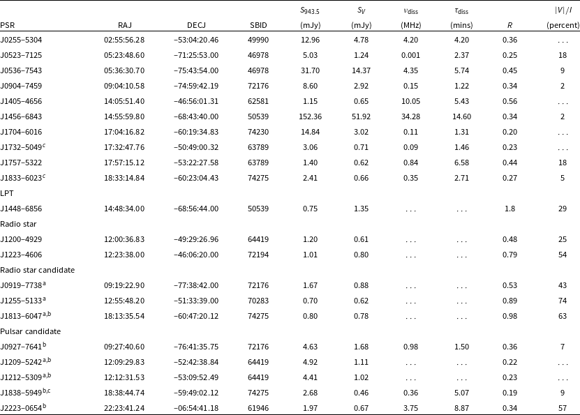
Out of 28 known pulsars detected in all analysed EMU tiles, we successfully detected 10 pulsars in their corresponding variance images within a DM range 8–157 pc cm $^{-3}$
. Their continuum flux density at 943.5 MHz (
$^{-3}$
. Their continuum flux density at 943.5 MHz ( $S_\mathrm{943.5}$
), variance flux (
$S_\mathrm{943.5}$
), variance flux ( $S_{V}$
), and Variability (R) are given in Table 2. In Figure 3, we show their detection in variance images (left panel) and dynamic spectra (right panel). These dynamic spectra span a duration of 10 h, except the SB 61946, with a total observing duration of five hours (last panel in Figure 4). Scintillation bandwidth and timescale for all detected known pulsars were estimated as described in Section 3.1.2 and are presented in Table 2. For pulsars whose proper motions are not known, we have used a nominal transverse velocity of 100 km s
$S_{V}$
), and Variability (R) are given in Table 2. In Figure 3, we show their detection in variance images (left panel) and dynamic spectra (right panel). These dynamic spectra span a duration of 10 h, except the SB 61946, with a total observing duration of five hours (last panel in Figure 4). Scintillation bandwidth and timescale for all detected known pulsars were estimated as described in Section 3.1.2 and are presented in Table 2. For pulsars whose proper motions are not known, we have used a nominal transverse velocity of 100 km s $^{-1}$
. The scintillation bandwidths
$^{-1}$
. The scintillation bandwidths $\nu_\mathrm{diss}$
and timescales
$\nu_\mathrm{diss}$
and timescales $\tau_\mathrm{diss}$
of three known pulsars (J0255–5304, J0536–7543, and J1456–6843) have been previously measured (Johnston et al. Reference Johnston, Nicastro and Koribalski1998). For PSRs J0536–7543 and J1456–6843, the scintillation bandwidth and timescale observed in EMU (at
$\tau_\mathrm{diss}$
of three known pulsars (J0255–5304, J0536–7543, and J1456–6843) have been previously measured (Johnston et al. Reference Johnston, Nicastro and Koribalski1998). For PSRs J0536–7543 and J1456–6843, the scintillation bandwidth and timescale observed in EMU (at $\sim$
1 GHz) are generally consistent with previous measurements. In contrast, PSR J0255–5304 exhibits a significantly broader scintillation bandwidth and longer timescale. The continuum source J1704–6019 was detected at RAJ = 17:04:16.82, DecJ =
$\sim$
1 GHz) are generally consistent with previous measurements. In contrast, PSR J0255–5304 exhibits a significantly broader scintillation bandwidth and longer timescale. The continuum source J1704–6019 was detected at RAJ = 17:04:16.82, DecJ = $-$
60:19:34.83. The positional offset between the continuum source J1704–6019 and the timing position of PSR J1704
$-$
60:19:34.83. The positional offset between the continuum source J1704–6019 and the timing position of PSR J1704 $-$
6016 has already been reported by Wang et al. (Reference Wang2023). The pronounced variability of the source is consistent with DISS at a DM of
$-$
6016 has already been reported by Wang et al. (Reference Wang2023). The pronounced variability of the source is consistent with DISS at a DM of $\sim$
50 pc cm
$\sim$
50 pc cm $^{-3}$
, reinforcing the association of the continuum source with PSR J1704
$^{-3}$
, reinforcing the association of the continuum source with PSR J1704 $-$
6016. PSR J0523–7125 was detected in the variance image despite its relatively high DM of 157 pc cm
$-$
6016. PSR J0523–7125 was detected in the variance image despite its relatively high DM of 157 pc cm $^{-3}$
. Its detection is due to its steep spectral index and pronounced variability on timescales of
$^{-3}$
. Its detection is due to its steep spectral index and pronounced variability on timescales of $\sim$
days (Wang et al. Reference Wang2022), consistent with the dynamic spectrum observed in the EMU data (Figure 3).
$\sim$
days (Wang et al. Reference Wang2022), consistent with the dynamic spectrum observed in the EMU data (Figure 3).
21 highly variable radio sources detected via variance imaging are listed in this table. Columns include source names, coordinates (RAJ $\&$
DECJ), schedule block ID (SBID), continuum flux densities at 943.5 MHz from EMU (
$\&$
DECJ), schedule block ID (SBID), continuum flux densities at 943.5 MHz from EMU ( $S_\mathrm{943.5}$
), variance flux (
$S_\mathrm{943.5}$
), variance flux ( $S_{v}$
), scintillation bandwidths (
$S_{v}$
), scintillation bandwidths ( $\nu_\mathrm{diss}$
) and timescales (
$\nu_\mathrm{diss}$
) and timescales ( $\tau_\mathrm{diss}$
) of detected known and new pulsars at
$\tau_\mathrm{diss}$
) of detected known and new pulsars at $\sim$
1 GHz, variability (R) defined as the ratio of variance flux (
$\sim$
1 GHz, variability (R) defined as the ratio of variance flux ( $S_{v}$
) to continuum flux densities (
$S_{v}$
) to continuum flux densities ( $S_\mathrm{943.5}$
), and circular polarisation fractions (
$S_\mathrm{943.5}$
), and circular polarisation fractions ( $V/I$
) if detected.
$V/I$
) if detected.
 $^\mathrm{a}$
With potential optical counterpart.
$^\mathrm{a}$
With potential optical counterpart. $^b$
Observed with Murriyang.
$^b$
Observed with Murriyang. $^c$
Not picked up by our selection criteria.
$^c$
Not picked up by our selection criteria.
Of the remaining 18 pulsars not detected in the variance images, 14 have DMs greater than 50 pc cm $^{-3}$
. For these pulsars, the expected scintillation bandwidths are narrow (
$^{-3}$
. For these pulsars, the expected scintillation bandwidths are narrow ( $\lesssim$ $0.15$
MHz), such that DISS is heavily averaged within the 24 MHz imaging channels, thereby suppressing measurable variance. Even at the highest frequency resolution available for EMU (1 MHz), the DISS of these pulsars is unlikely to be resolved, and their relatively low flux densities (
$0.15$
MHz), such that DISS is heavily averaged within the 24 MHz imaging channels, thereby suppressing measurable variance. Even at the highest frequency resolution available for EMU (1 MHz), the DISS of these pulsars is unlikely to be resolved, and their relatively low flux densities ( $\lesssim$ $1.5$
mJy) further reduce the likelihood of detection. The remaining four low-DM pulsars (PSRs J0540–7125, J1232–4742, J1240–4124, and J2222–0137) all have flux densities below 1 mJy, making them challenging to detect in variance images due to limited sensitivity. In addition, PSR J0540–7125 is located near a bright double-lobed source, where residual sidelobes further hinder reliable variance detection. PSR J2222–0137 lies close to the edge of beam 35 (SB61946), where the primary beam response and sensitivity are significantly reduced.
$1.5$
mJy) further reduce the likelihood of detection. The remaining four low-DM pulsars (PSRs J0540–7125, J1232–4742, J1240–4124, and J2222–0137) all have flux densities below 1 mJy, making them challenging to detect in variance images due to limited sensitivity. In addition, PSR J0540–7125 is located near a bright double-lobed source, where residual sidelobes further hinder reliable variance detection. PSR J2222–0137 lies close to the edge of beam 35 (SB61946), where the primary beam response and sensitivity are significantly reduced.
In addition to known pulsars, we also detected the known long period transient (LPT) source J1448–6856 (Anumarlapudi et al. Reference Anumarlapudi2025), as well as two radio stars. Along with pronounced temporal variability, J1448–6856 exhibits significant frequency-dependent variability, making it stand out clearly in the variance image. The detected radio stars (J1200–4929 and J1223–4606) are listed in the Sydney Radio Star CatalogueFootnote c and were independently identified in previous studies through variability and circular polarisation searches (Driessen et al. Reference Driessen2024). Their re-detection further supports the reliability of variance imaging in uncovering highly variable stellar radio sources.
4.2. Pulsar discoveries
A strong pulsar candidate (J2223–0654) was identified in beam 05 of the tile SB 61946 (see Figure 2). The dynamic spectrum of this candidate shows flux density modulation consistent with DISS. The continuum source is $\sim$
60% circularly polarised with no optical counterpart. We observed this candidate using the UWL receiver on Murriyang, the Parkes radio telescope (see Section 2.2 for details) and detected a periodic signal with a period of
$\sim$
60% circularly polarised with no optical counterpart. We observed this candidate using the UWL receiver on Murriyang, the Parkes radio telescope (see Section 2.2 for details) and detected a periodic signal with a period of $\sim$
85.7 ms and a DM of 19.4 pc cm
$\sim$
85.7 ms and a DM of 19.4 pc cm $^{-3}$
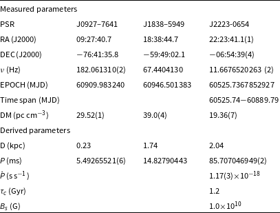
. Follow-up observations with Murriyang confirmed the discovery of an isolated pulsar (hereafter designated as PSR J2223–0654), and an initial timing solution has been obtained (see Table 3).
$^{-3}$
. Follow-up observations with Murriyang confirmed the discovery of an isolated pulsar (hereafter designated as PSR J2223–0654), and an initial timing solution has been obtained (see Table 3).
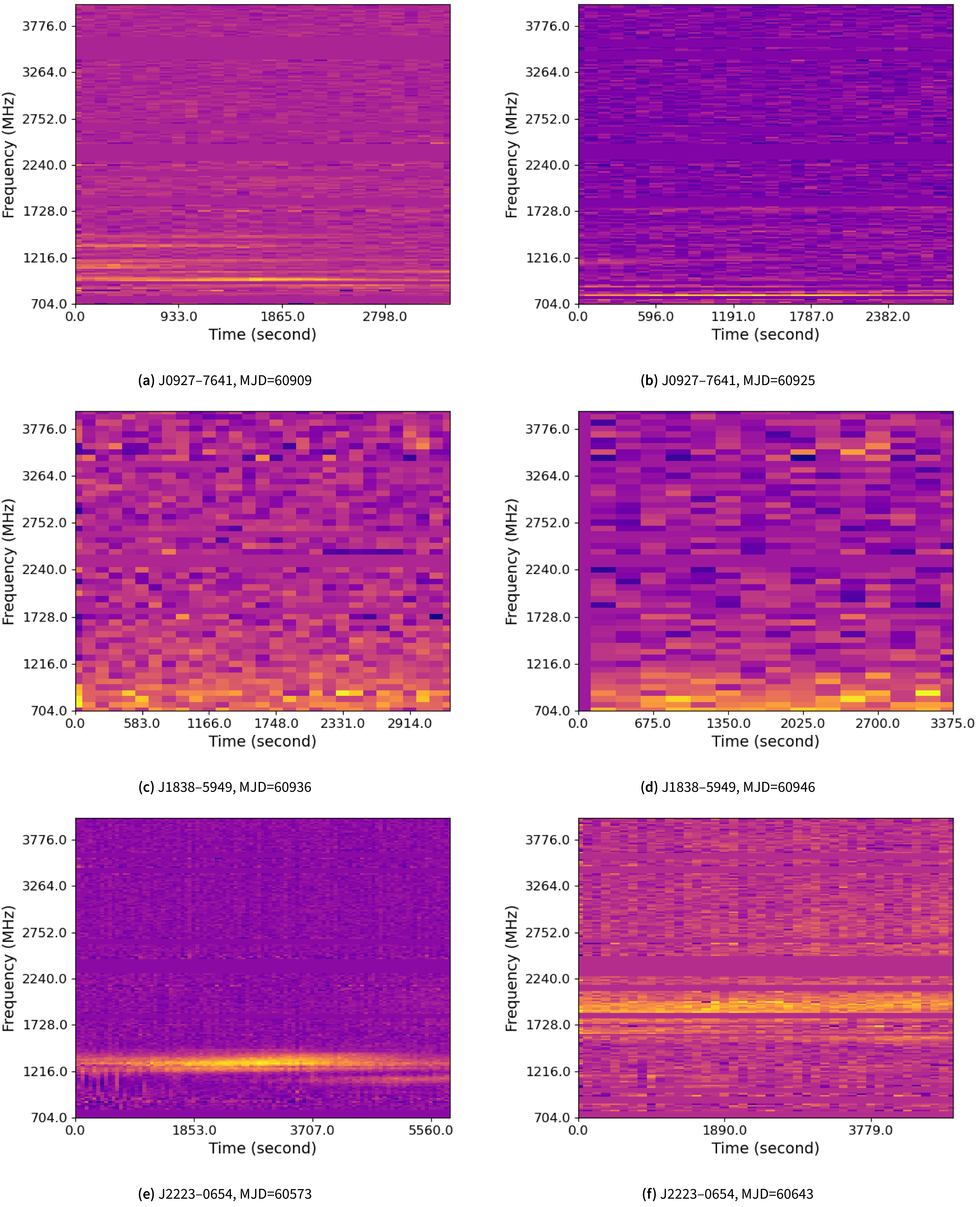
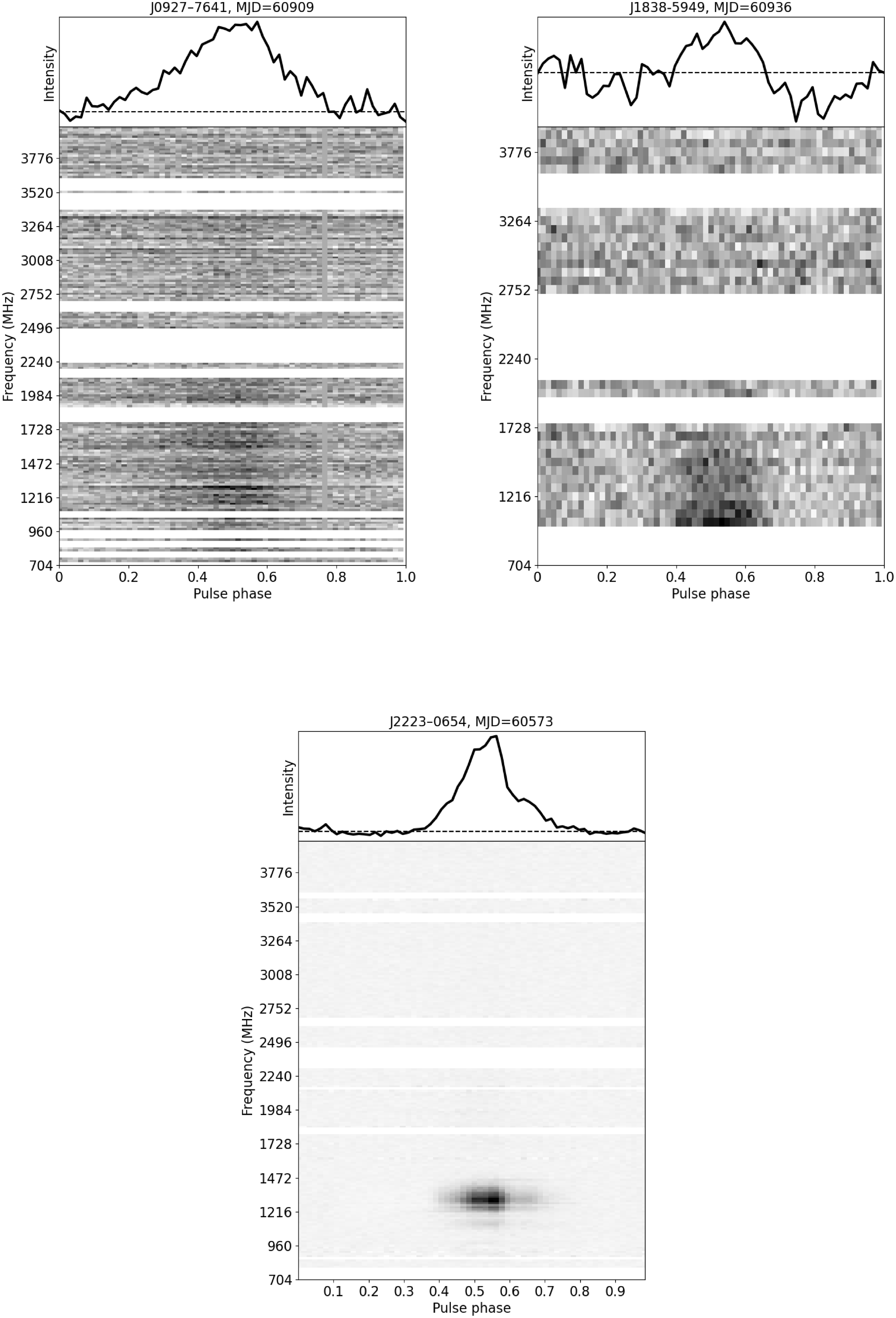
The wideband dynamic spectra of PSR J2223–0654 at two different Murriyang observing epochs are shown in Figure 5. These observations at different epochs show that the flux density of the pulsar varies significantly across a wide band (704–4 032 MHz) and exhibits clear frequency-dependent intensity variations, which is a characteristic of strong DISS. For example, in one observation (Figure 5(e)), the pulsar can only be detected within a narrow spectral window ( $\sim$
1000–1472 MHz), while in another (Figure 5(f)), it appears to be brighter at higher frequencies and within a wider bandwidth (
$\sim$
1000–1472 MHz), while in another (Figure 5(f)), it appears to be brighter at higher frequencies and within a wider bandwidth ( $\sim$
1500–2250 MHz).
$\sim$
1500–2250 MHz).
Measured and derived parameters of pulsar discoveries with current timing observations.

Another pulsar candidate (J0927–7641) was identified in beam 27 of the tile SB 72176. It exhibits strong variability ( $\gt$
30%) and is clearly distinct from the other sources in the beam (Figure 2). The continuum source has Stokes I peak flux density of
$\gt$
30%) and is clearly distinct from the other sources in the beam (Figure 2). The continuum source has Stokes I peak flux density of $4.55\pm 0.06$
mJy and Stokes V peak flux density of
$4.55\pm 0.06$
mJy and Stokes V peak flux density of $0.34\pm 0.02$
mJy, and has no optical counterpart with
$0.34\pm 0.02$
mJy, and has no optical counterpart with $|V|/I\approx7.5\pm 0.5$
%. We observed this candidate with Murriyang using the same observational setup as described above and discovered a pulsar with a spin period of 5.492 ms and a DM of 29.5 pc cm
$|V|/I\approx7.5\pm 0.5$
%. We observed this candidate with Murriyang using the same observational setup as described above and discovered a pulsar with a spin period of 5.492 ms and a DM of 29.5 pc cm $^{-3}$
. The wideband dynamic spectrum of PSR J0927–7641 is shown in Figure 5(a) and b, which shows strong scintillation at
$^{-3}$
. The wideband dynamic spectrum of PSR J0927–7641 is shown in Figure 5(a) and b, which shows strong scintillation at $\sim$
1 GHz. Whether this is an isolated MSP or an MSP in a binary system is to be determined. So far, we have conducted four observations (at MJD 60910, 60913, 60920, and 60925), during which we observed an almost linear decrease in the pulsar’s measured spin period. This indicates that PSR J0927–7641 is likely in a binary system with an orbital period on the order of several tens of days. Follow-up observations of this pulsar are underway to measure its orbital parameters and obtain a coherent timing solution.
$\sim$
1 GHz. Whether this is an isolated MSP or an MSP in a binary system is to be determined. So far, we have conducted four observations (at MJD 60910, 60913, 60920, and 60925), during which we observed an almost linear decrease in the pulsar’s measured spin period. This indicates that PSR J0927–7641 is likely in a binary system with an orbital period on the order of several tens of days. Follow-up observations of this pulsar are underway to measure its orbital parameters and obtain a coherent timing solution.
A third pulsar candidate (J1838–5949) was identified in beam 21 of tile SB74275. With targeted observations using Murriyang, we discovered a pulsar with a spin period of 14.828 ms and a DM of 39.0 pc cm $^{-3}$
. Unlike PSRs J0927–7641 and J2223–0654, J1838–5949 did not meet the
$^{-3}$
. Unlike PSRs J0927–7641 and J2223–0654, J1838–5949 did not meet the $5\sigma$
variability threshold. Instead, it was identified as a candidate because it was detected in both the variance and circular polarisation images (Section 3.2). The associated continuum source is approximately 9% circularly polarised. Follow-up observations with Murriyang (Figure 5(c) and (d)) indicate that J1838–5949 is not strongly scintillating. Rather, it is likely a pulsar with an extremely steep radio spectrum, consistent with its dynamic spectrum observed in the EMU data. Current Murriyang observations also suggest that J1838–5949 is likely in a binary system, and follow-up observations are ongoing. The measured and derived parameters of new pulsars with current timing observation are presented in Table 3.
$5\sigma$
variability threshold. Instead, it was identified as a candidate because it was detected in both the variance and circular polarisation images (Section 3.2). The associated continuum source is approximately 9% circularly polarised. Follow-up observations with Murriyang (Figure 5(c) and (d)) indicate that J1838–5949 is not strongly scintillating. Rather, it is likely a pulsar with an extremely steep radio spectrum, consistent with its dynamic spectrum observed in the EMU data. Current Murriyang observations also suggest that J1838–5949 is likely in a binary system, and follow-up observations are ongoing. The measured and derived parameters of new pulsars with current timing observation are presented in Table 3.
Time- and frequency-averaged pulse profiles (top panels) and time-averaged spectra (bottom panels) for the new pulsars are shown in Figure 6. The scintillation bandwidth and timescale at $\sim$
1 GHz for the new pulsars were estimated as described in Section 3.1.2. Because their distances are unknown, we adopt DM-based distances derived using the YMW16 model for the Galactic distribution of free electrons (Yao et al. Reference Yao, Manchester and Wang2017) and are listed in Table 3. The estimated scintillation bandwidths of PSRs J0927–7641 and J2223–0654 are broadly consistent with the scintillation structure observed in EMU at 943.5 MHz.
$\sim$
1 GHz for the new pulsars were estimated as described in Section 3.1.2. Because their distances are unknown, we adopt DM-based distances derived using the YMW16 model for the Galactic distribution of free electrons (Yao et al. Reference Yao, Manchester and Wang2017) and are listed in Table 3. The estimated scintillation bandwidths of PSRs J0927–7641 and J2223–0654 are broadly consistent with the scintillation structure observed in EMU at 943.5 MHz.
Murriyang dynamic spectra of PSRs J0927–7641, J1838–5949 and J2223–0654, which show the flux density of pulsars as a function of time and frequency.

Top panels: Time and frequency averaged pulse profiles of PSRs J0927–7641, J1838–5949, and J2223–0654. Bottom panels: Time averaged spectrum for each pulsar across the whole UWL band.

4.3. Radio star candidates
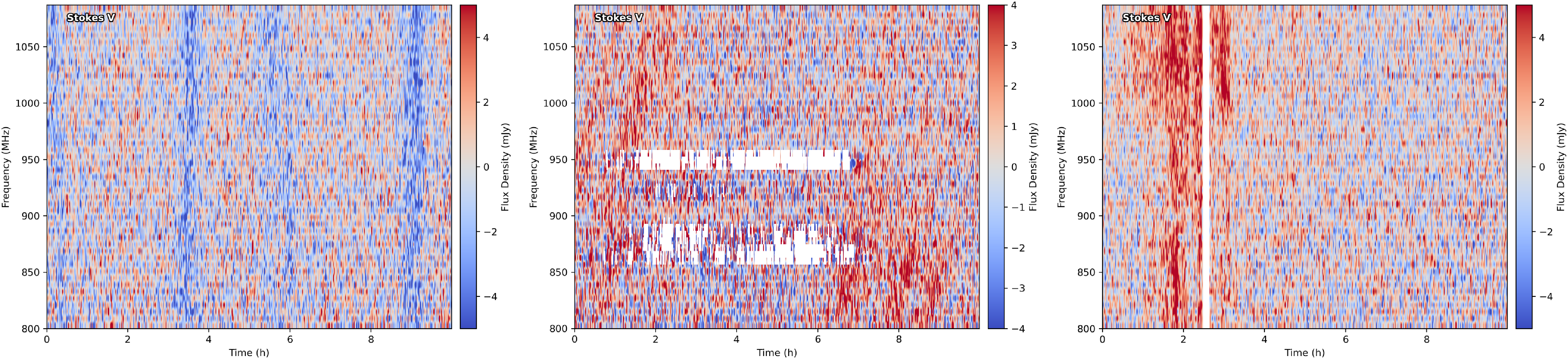
Three of our candidates, J0919–7738, J1255–5133 and J1813–6047, exhibit strong circular polarisation and are associated with optical counterparts. For J1813–6047, a possible periodic double-peaked structure with a period of $\sim5.8$
hr is evident in the dynamic spectrum of the circular polarisation (Figure 7), suggesting it may be a flaring star. J0919–7738 and J1255–5133 also show clear variability in their dynamic spectra, although no periodicity can be established with the current data. A detailed investigation of the optical companions to these candidate radio stars is beyond the scope of this work. Follow-up radio observations will be necessary to better characterise the nature of their radio emission.
$\sim5.8$
hr is evident in the dynamic spectrum of the circular polarisation (Figure 7), suggesting it may be a flaring star. J0919–7738 and J1255–5133 also show clear variability in their dynamic spectra, although no periodicity can be established with the current data. A detailed investigation of the optical companions to these candidate radio stars is beyond the scope of this work. Follow-up radio observations will be necessary to better characterise the nature of their radio emission.
Dynamic spectra of the circular polarisation of radio star candidates: J1813–6047 (left), J1255–5133 (middle), J0919–7738 (right).

Although unlikely to be a pulsar, we conducted follow-up observations of candidate J1813–6047 using Murriyang. A single observation of J1813–6047 was carried out with an integration time of 2204 s. No periodic signal was detected from the source across a DM range of 0 to 500 pc cm $^{-3}$
.
$^{-3}$
.
4.4. Other pulsar candidates
In addition to PSRs J0927–7641, J1838—5949, and J2223–0654, we conducted Murriyang follow-up observations of pulsar candidates: J1209–5242 and J1212–5309. The observational setup and pulsar searching strategy were the same as described above, with an integration time of approximately 1 hr. No periodic signals were detected from these sources over a DM range of 0–500 pc cm $^{-3}$
. Compared with PSRs J0927–7641 and J2223–0654, these pulsar candidates show lower variabilities, although DISS-like structures can be observed in their dynamic spectra (Figure 4). Repeated observations might be necessary to reveal their periodic signals.
$^{-3}$
. Compared with PSRs J0927–7641 and J2223–0654, these pulsar candidates show lower variabilities, although DISS-like structures can be observed in their dynamic spectra (Figure 4). Repeated observations might be necessary to reveal their periodic signals.
5. Discussion and conclusion
In this pilot study, we applied the variance imaging technique to EMU data observed at high Galactic latitude regions, where pulsars are expected to have lower DM and broader scintillation bandwidth and timescales, enabling the creation of variance images using a relatively small number of frequency channels and time integrations. Within the total FoV, of the 28 known pulsars detected in continuum images, 10 were also detected in corresponding variance images. The targeted pulsation searches of four compact, highly scintillating pulsar candidates identified through variance imaging led to the discovery of two new pulsars: J2223–0654 with a period of 85.707 ms and a DM of 19.4 pc cm $^{-3}$
, and J0927–7641 with a period of 5.492 ms and a DM of 29.5 pc cm
$^{-3}$
, and J0927–7641 with a period of 5.492 ms and a DM of 29.5 pc cm $^{-3}$
. Additionally, a third pulsar, J1838–5949, was discovered in the variance image due to its steep radio spectrum. It has a period of 14.828 ms and a DM of 39.0 pc cm
$^{-3}$
. Additionally, a third pulsar, J1838–5949, was discovered in the variance image due to its steep radio spectrum. It has a period of 14.828 ms and a DM of 39.0 pc cm $^{-3}$
, and exhibit high degree of circular polarisation.
$^{-3}$
, and exhibit high degree of circular polarisation.
Our discoveries demonstrated the effectiveness of variance imaging in distinguishing highly scintillating pulsars from other compact radio sources. This method eliminates the need for pixel-by-pixel blind pulsar surveys with either single dishes or tied-array beams, as well as the computationally intensive processing of large volumes of high-time-resolution data. Instead, it enables efficient, targeted deep and wideband searches that maximise the likelihood of detecting elusive pulsars such as those with large duty cycles, strong scintillation, or in compact binary systems. Beyond pulsars, variance imaging also holds promise for identifying LPT candidates and highly variable stellar radio sources (e.g. flare stars).
The next step is to apply the variance imaging technique across the full EMU sky at intermediate and high Galactic latitudes. We also plan to generate variance images at both higher and lower time and frequency resolutions to explore a broader range of DM. In addition to lower frequency and time resolution required to create variance images at high Galactic latitudes, we expect lower sky temperature and reduced source confusion due to the lack of extended radio emission, which further simplifies the process and enhances the sensitivity. This potentially enables the detection of MSPs and pulsars in compact binaries, which were likely missed by previous shallow and single-epoch pulsar surveys at high Galactic latitudes (e.g. Keith et al. Reference Keith2010; Keane et al. Reference Keane2018).
In the Galactic plane, the dense ISM leads to high DMs, which reduce scintillation bandwidths and timescales, often below the spectral and temporal resolution of a given continuum survey. This suppresses detectable variability due to DISS at around 1 GHz, limiting the effectiveness of variance imaging for typical high-DM pulsars. Additionally, the crowded sky and diffuse radio emission (e.g. SNRs, PNe, HII regions) increase the likelihood of false positives due to image artefacts and source confusion. High-frequency continuum surveys such as the Very Large Array Sky Survey (VLASS, 2–4 GHz; Lacy et al. Reference Lacy2020), Deep Synoptic Array 2000-antenna (DSA-2000, 0.7–2 GHz; Hallinan et al. Reference Hallinan2019), and future SKA-mid surveys (Prandoni & Seymour Reference Prandoni and Seymour2015) offer better avenues for pulsar discoveries with variance imaging in the Galactic plane.
While our pilot survey demonstrated that variance imaging and our source selection strategy are effective and efficient for identifying pulsars, it also revealed several challenges. A key challenge in variance imaging is that snapshot images are constructed across multiple frequency channels and time integrations, each associated with a different point spread function (PSF) due to the frequency- and time-dependent nature of the uv-coverage. As a result, compact sources may appear elliptical and rotate across successive snapshots. When pixel-wise variance is computed from such images, these PSF variations can lead the sources to appear ring-like or wing-like in the variance image, often characterised by suppressed variance at around the source central pixels and elevated variance in the outer wings. Such morphological artefacts can result in false positives and reduce our sensitivity to faint sources. Correcting for the time- and frequency-dependent PSF is challenging, as it varies in complex ways due to flagging and baseline projection. In future pipelines, we plan to test convolving snapshot images to a common beam and assess its effectiveness for identifying scintillating sources compared with our current approach.
Another critical factor affecting the fidelity of variance images is the presence of bright sources, either within or outside the primary beam. Even when a bright source lies outside the imaged tile, its response can leak into the snapshot images through the sidelobes of the primary beam. Although these sidelobes are not expected to scintillate over time, they can exhibit strong frequency-dependent variations, introducing spurious compact and extended structures in the variance image that could be interpreted as artificially variable sources (see Figure 1). Additionally, bright sources within the primary beam can also produce residual sidelobes if not accurately modelled and subtracted from the visibilities. These residual sidelobe patterns introduce artefacts in the variance image around bright sources and can act as false positives. To address this, we are developing additional steps in our pipeline. For bright out-of-beam sources, we will apply the source peeling technique (e.g. Noordam Reference Noordam and Oschmann2004; Williams et al. Reference Williams, Allers, Biller and Vos2019) to subtract their contributions from the visibilities, with source locations identified from shallow surveys such as the Rapid ASKAP Continuum Survey (RACS; McConnell et al. Reference McConnell2020; Duchesne et al. Reference Duchesne2025). We also plan to apply phase and amplitude self-calibration to mitigate sidelobes from bright in-beam sources.
Finally, we plan to transition from CASA’s tclean to the WSClean imager (Offringa et al. Reference Offringa2014), which offers significant computational advantages. By replacing the w-projection algorithm (tclean) with the w-stacking GRIDDING algorithm (WSClean), we anticipate three major benefits: (1) improved scalability and multinode parallelism for large datasets, (2) execution efficiency and reduced processing times, particularly in the deep sky model and snapshot imaging stages, and (3) high fidelity images with reduced noise (e.g. An et al. Reference An, Lao, Xu, Lu, Wang, Murphy, Kaplan and Guo2023).
Acknowledgements
We thank Juntao Bai, Joshua Pritchard, Andrew Zic, and Tim Galvin for the useful discussions. Murriyang, CSIRO’s Parkes radio telescope, is part of the Australia Telescope National FacilityFootnote d (ATNF) which is funded by the Australian Government for operation as a National Facility managed by the Commonwealth Scientific and Industrial Research Organisation (CSIRO). The ATNF Pulsar Catalogue (https://www.atnf.csiro.au/research/pulsar/psrcat/) was used for this work. This scientific work uses data obtained from Inyarrimanha Ilgari Bundara, the CSIRO Murchison Radio-astronomy Observatory. We acknowledge the Wajarri Yamaji People as the Traditional Owners and native title holders of the Observatory site. CSIRO’s ASKAP radio telescope is part of the Australia Telescope National Facility (https://ror.org/05qajvd42). Operation of ASKAP is funded by the Australian Government with support from the National Collaborative Research Infrastructure Strategy. ASKAP uses the resources of the Pawsey Supercomputing Research Centre. Establishment of ASKAP, Inyarrimanha Ilgari Bundara, the CSIRO Murchison Radio-astronomy Observatory and the Pawsey Supercomputing Research Centre are initiatives of the Australian Government, with support from the Government of Western Australia and the Science and Industry Endowment Fund. The data processing was performed on the OzSTARFootnote e national facility at Swinburne University of Technology. The OzSTAR program receives funding in part from the Astronomy National Collaborative Research Infrastructure Strategy (NCRIS) allocation provided by the Australian Government, and from the Victorian Higher Education State Investment Fund (VHESIF) provided by the Victorian Government.
Data availability statement
The observations from Murriyang are publicly available from https://data.csiro.au/domain/atnf after an 18 month embargo period. This study made use of archival ASKAP data obtained from the CASDA https://data.csiro.au/domain/casdaObservation.









 Open access

