


Impact Statement
In the context of sustainability, circular material systems require the development of alternatives to fossil-based and energy-consuming materials. One attractive path is less-energy-demanding materials made from biobased resources. Many natural materials obtain impressive properties by a hierarchical structure, where nanosized subassemblies appear in a structured manner. In this work, we combine experimental and numerical work to demonstrate how different channel flow geometries can be used to organise the most abundant of such subassemblies, cellulose nanofibrils, in aligned structures. The aligned structures can, after further processing such as gelation and drying, develop into high-performance engineering materials.
1. Introduction
Dispersed particles of micrometric ( $10^{-6}$
m) and nanometric (
$10^{-6}$
m) and nanometric ( $10^{-9}$
m) size are ubiquitous in the biological world, and are promising building blocks for developing sustainable, biocompatible materials (Solomon & Spicer Reference Solomon and Spicer2010). A few examples are biopolymers and colloids such as cellulose nanofibrils (CNFs) in trees, algae and bacteria (Moon et al. Reference Moon, Martini, Nairn, Simonsen and Youngblood2011), chitin nanofibrils in animals (Ehrlich Reference Ehrlich2010), silk nanofibrils from spiders and silkworms (Ling et al. Reference Ling, Qin, Li, Huang, Kaplan and Buehler2017), protein nanofibrils from eggs (Humblet-Hua et al. Reference Humblet-Hua, Sagis and van der Linden2008) and milk (Loveday et al. Reference Loveday, Su, Rao, Anema and Singh2012) and viruses like tobaccomosaic virus (Nemoto et al. Reference Nemoto, Schrag, Ferry and Fulton1975) or coronavirus (Kanso et al. Reference Kanso, Piette, Hanna and Giacomin2020).
$10^{-9}$
m) size are ubiquitous in the biological world, and are promising building blocks for developing sustainable, biocompatible materials (Solomon & Spicer Reference Solomon and Spicer2010). A few examples are biopolymers and colloids such as cellulose nanofibrils (CNFs) in trees, algae and bacteria (Moon et al. Reference Moon, Martini, Nairn, Simonsen and Youngblood2011), chitin nanofibrils in animals (Ehrlich Reference Ehrlich2010), silk nanofibrils from spiders and silkworms (Ling et al. Reference Ling, Qin, Li, Huang, Kaplan and Buehler2017), protein nanofibrils from eggs (Humblet-Hua et al. Reference Humblet-Hua, Sagis and van der Linden2008) and milk (Loveday et al. Reference Loveday, Su, Rao, Anema and Singh2012) and viruses like tobaccomosaic virus (Nemoto et al. Reference Nemoto, Schrag, Ferry and Fulton1975) or coronavirus (Kanso et al. Reference Kanso, Piette, Hanna and Giacomin2020).
Amongst these, CNFs (diameter ranging from 2 to 100 nm) are of particular interest, since they are lightweight, available in abundance, renewable and biocompatible, and have high mechanical performance (Ling, Kaplan & Buehler Reference Ling, Kaplan and Buehler2018; Li et al. Reference Li, Chen, Brozena, Zhu, Xu, Driemeier, Dai, Rojas, Isogai, Wågberg and Hu2021). With control of their hierarchical structure, nanofibrils have been used in the fabrication of macroscopic materials ranging from macrofibres (Iwamoto, Isogai & Iwata Reference Iwamoto, Isogai and Iwata2011) and composites (Capadona et al. Reference Capadona, Van Den Berg, Capadona, Schroeter, Rowan, Tyler and Weder2007) to thin films (Lagerwall et al. Reference Lagerwall, Schütz, Salajkova, Noh, Hyun Park, Scalia and Bergström2014), porous membranes and gels (Håkansson et al. Reference Håkansson, Henriksson, de la Peña Vázquez, Kuzmenko, Markstedt, Enoksson and Gatenholm2016). Thus, as renewable, biocompatible building blocks, CNFs can be a key ingredient for circular material systems.
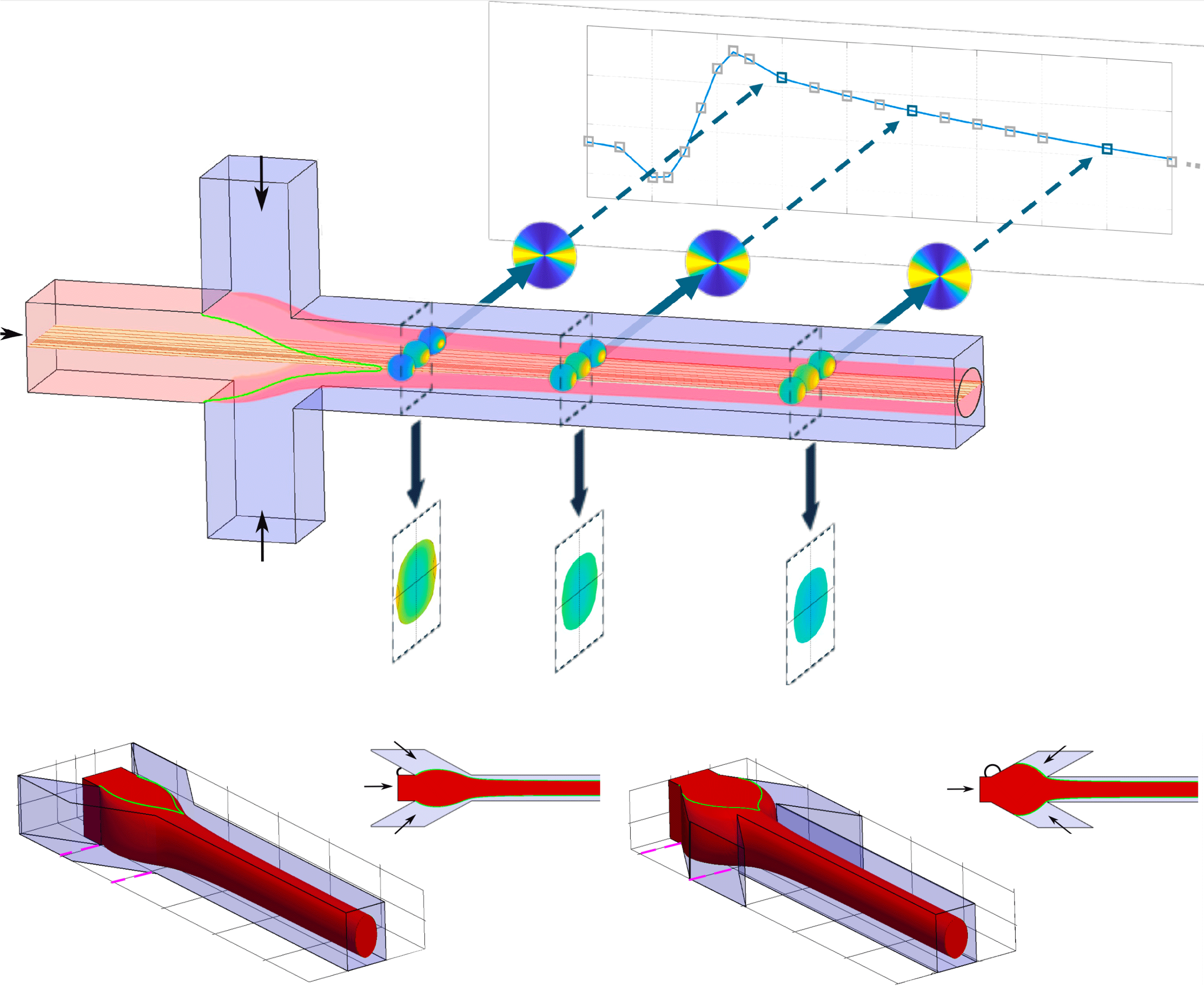
One assembly technology that has shown great potential for controlling and regulating nanofibril assembly is hydrodynamic assembly (Nunes et al. Reference Nunes, Tsai, Wan and Stone2013; Hou et al. Reference Hou, Zhang, Santiago, Alvarez, Ribas, Jonas, Weiss, Andrews, Aizenberg and Khademhosseini2017). A method of particular interest is flow focusing (Anna, Bontoux & Stone Reference Anna, Bontoux and Stone2003), which is illustrated in figure 1. Here, a core flow of nanofibril colloidal dispersion is focused by its own solvent through outer sheath flows, to first align fibrils, and then use colloidal chemistry to lock them in a gel thread that can be dried into a filament (Håkansson et al. Reference Håkansson, Fall, Lundell, Yu, Krywka, Roth, Santoro, Kvick, Prahl Wittberg, Wågberg and Söderberg2014; Kamada et al. Reference Kamada, Mittal, Söderberg, Ingverud, Ohm, Roth, Lundell and Lendel2017). The properties of the assembled nanofibril filaments (e.g. stiffness, strength and biological and electrical functions) are, to a large extent, determined by the alignment of the fibrils. By controlling the alignment and orientation of nanofibrils in the dispersion (Doi & Edwards Reference Doi and Edwards1988; Jeffery Reference Jeffery1922; Tucker III Reference Tucker2022), these nanofibril filaments could indeed form the foundation for sustainable material technologies. Engineering sustainable materials from natural building blocks of colloidal particles (e.g. cellulose or protein nanofibrils) using microfluidic flows requires an in-depth understanding of the behaviour of colloidal particle dispersions under flowing conditions (Calabrese, Shen & Haward Reference Calabrese, Shen and Haward2023).
In order to achieve successful assembly and alignment of fibrils, the flow must be tuned to form a thread, and there must be extensional or sheared flow that aligns the fibrils. In a combined numerical and experimental study of the flow in the geometry of figure 1(a), Gowda et al. (Reference Gowda. V, Brouzet, Lefranc, Söderberg and Lundell2019) showed (i) that a crucial aspect for good thread formation is Korteweg stresses (Korteweg Reference Korteweg1901) in regions of concentration gradients, which give rise to an effective interfacial tension (EIT) between the colloidal dispersion in the core and its solvent in the sheath flows (Truzzolillo et al. Reference Truzzolillo, Roger, Dupas, Mora and Cipelletti2015), and (ii) that if the EIT is introduced in computational fluid dynamic simulations, an excellent agreement is obtained between the simulated flow fields and experimental measurements acquired with optical coherence tomography. In a follow-up study, Gowda et al. (Reference Gowda, Rydefalk, Söderberg and Lundell2021) further demonstrated the accuracy of the numerical flow model for all geometries of figure 1(a–e), where the confluence angle $\beta$
between the core and sheath flows is varied between 30
$\beta$
between the core and sheath flows is varied between 30 $^\circ$
and 150
$^\circ$
and 150 $^\circ$
.
$^\circ$
.
For fibril alignment, the numerical flow fields were used as input to alignment simulations based on a Smoluchowski equation for the orientation distribution function (Doi & Edwards, Reference Doi and Edwards1988; Tucker III, Reference Tucker2022), and it was shown that the alignment observed by small-angle X-ray scattering (SAXS) measurements in the first geometry ( $\beta = 90^\circ$
; figure 1
a) could be reproduced by a two-fraction model (Gowda et al. Reference Gowda, Rosén, Roth, Söderberg and Lundell2022). This two-fraction model is a coarse approximation of the actual dispersion, but it was found to be sufficient for approximating the continuous length distribution of the fibrils.
$\beta = 90^\circ$
; figure 1
a) could be reproduced by a two-fraction model (Gowda et al. Reference Gowda, Rosén, Roth, Söderberg and Lundell2022). This two-fraction model is a coarse approximation of the actual dispersion, but it was found to be sufficient for approximating the continuous length distribution of the fibrils.
In this work, we expand on previous work and gain insights into how flow geometry affects thread formation and fibril alignment. First, a brief summary of the methods used is given in § 2. Four sets of results are presented in § 3. The first set is a comparison between numerical and experimental alignment data for the geometries with confluence angles $\beta =$
90
$\beta =$
90 $^\circ$
, 60
$^\circ$
, 60 $^\circ$
and 120
$^\circ$
and 120 $^\circ$
(figure 1
a–c). In the second set of results, the numerical alignment model is used to compare fibril alignment for all five confluence angle geometries. The third set is a numerical study of the flow in eight new flow geometries where the channel aspect ratio is varied and/or contractions are added in the core and/or sheath-flow channels. The fourth and final set of results uses the simulated flow in the eight new geometries to investigate thread formation and fibril alignment. The mean alignment at each streamwise position and the variation over the channel cross-section are evaluated. Finally, the conclusions are summarised in § 4.
$^\circ$
(figure 1
a–c). In the second set of results, the numerical alignment model is used to compare fibril alignment for all five confluence angle geometries. The third set is a numerical study of the flow in eight new flow geometries where the channel aspect ratio is varied and/or contractions are added in the core and/or sheath-flow channels. The fourth and final set of results uses the simulated flow in the eight new geometries to investigate thread formation and fibril alignment. The mean alignment at each streamwise position and the variation over the channel cross-section are evaluated. Finally, the conclusions are summarised in § 4.
2. Numerical and experimental methods
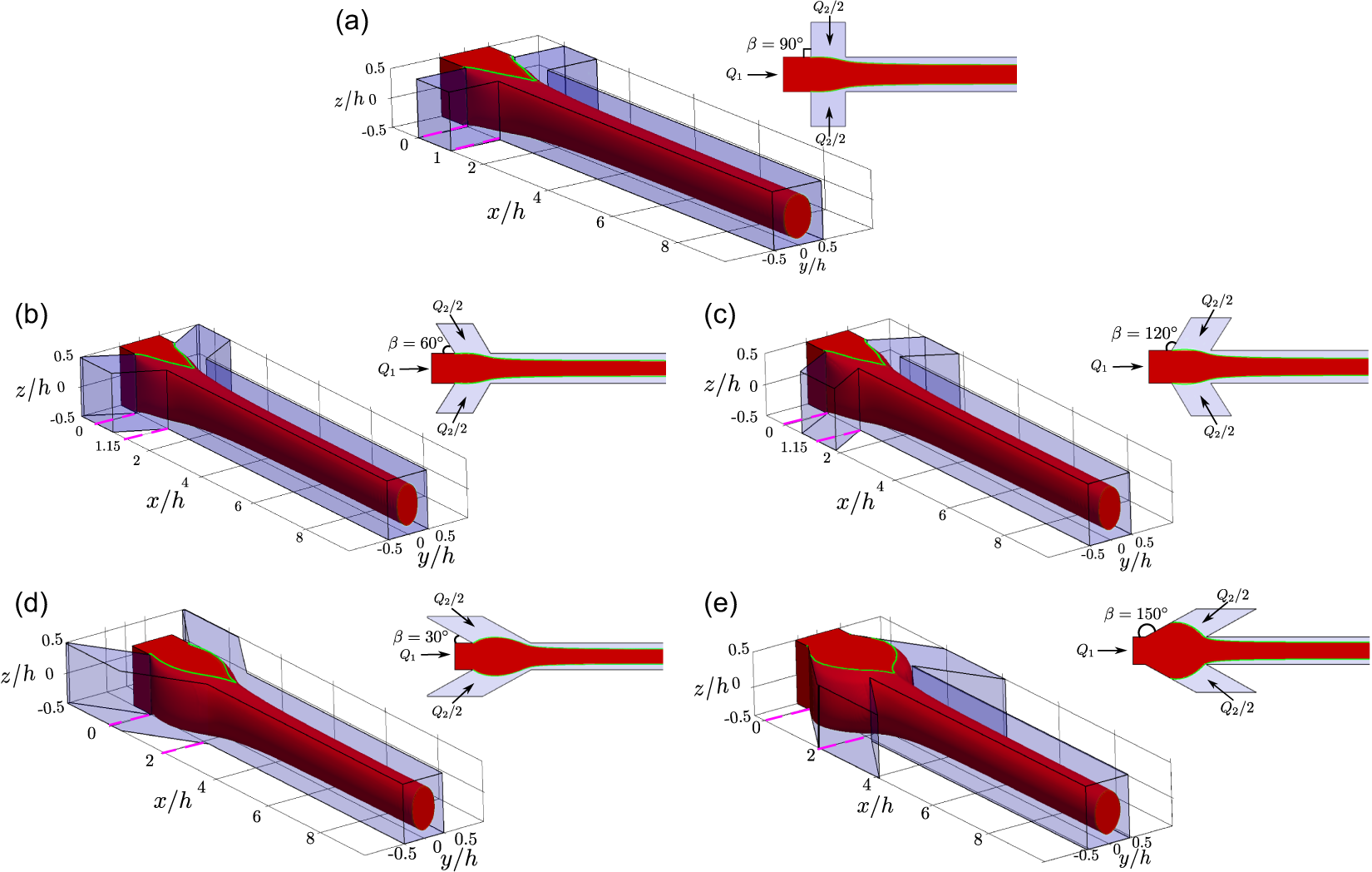
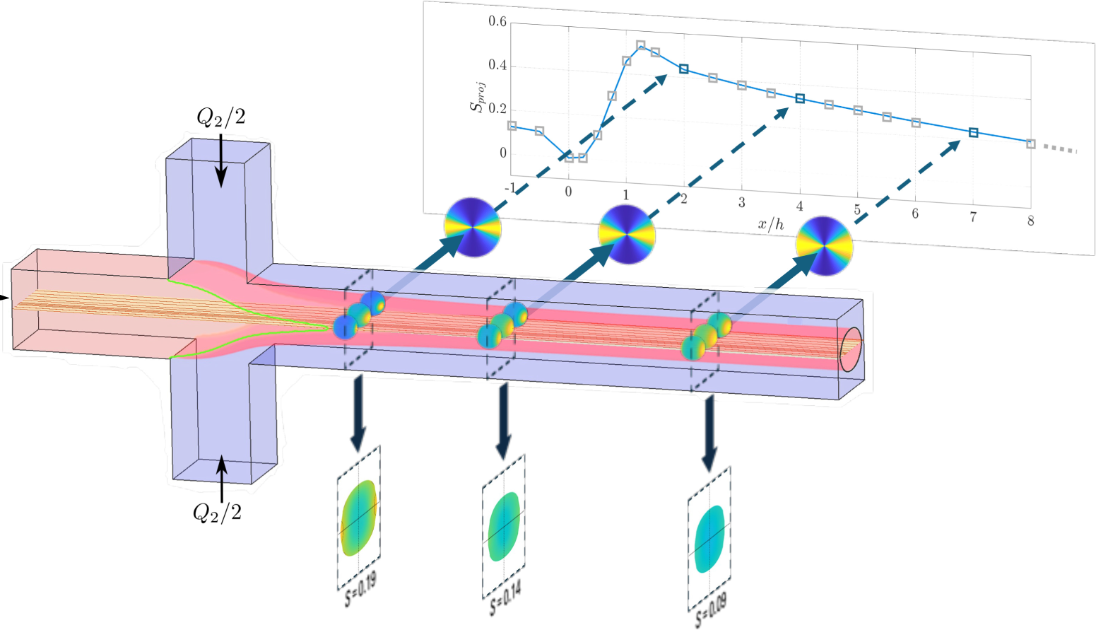
(a–e) Schematic illustration of various flow-focusing geometries. As seen from the top views, the side inlet channel arms join the main central channel at a confluence angle $\beta$
varying between
$\beta$
varying between $30^\circ$
and
$30^\circ$
and $150^\circ$
. The core fluid, denoted by red colour, enters the main central inlet channel arm with a volumetric flow rate
$150^\circ$
. The core fluid, denoted by red colour, enters the main central inlet channel arm with a volumetric flow rate $Q_{1}$
. The sheath fluid, represented by light-blue colour, enters from the side inlet channel arms with a flow rate of
$Q_{1}$
. The sheath fluid, represented by light-blue colour, enters from the side inlet channel arms with a flow rate of $Q_{2}/2$
from each side. The cross-section of the central channel arm in all these geometrical configurations is square with sidelength
$Q_{2}/2$
from each side. The cross-section of the central channel arm in all these geometrical configurations is square with sidelength $h$
.
$h$
.
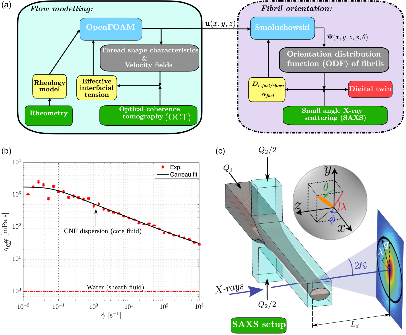
(a) Schematic illustration of the connection between flow modelling simulations and fibril orientation. Green blocks denote the experimental methods: rheometry, optical coherence tomography and SAXS. Yellow blocks indicate the variables used to calibrate the flow and fibril orientation numerical models represented by blue blocks. Grey blocks show the output features used for comparing experimental measurements and numerical model results. Red block indicates the digital twin developed through fibril orientation modelling. Velocity fields $\textbf {u}(x, y, z)$
obtained from flow modelling are the main input to fibril orientation modelling. (b) Shear viscosity measurements of core and sheath fluids. Red markers show the measured rheology of the CNF dispersion used in the present work, modelled using a non-Newtonian Carreau rheology model (equation (2.1)). The solid black line represents the Carreau fit, while the dash-dotted red line shows the viscosity of sheath fluid water. (c) Illustration of SAXS set-up. An X-ray beam traverses the flow-focusing geometry along the
$\textbf {u}(x, y, z)$
obtained from flow modelling are the main input to fibril orientation modelling. (b) Shear viscosity measurements of core and sheath fluids. Red markers show the measured rheology of the CNF dispersion used in the present work, modelled using a non-Newtonian Carreau rheology model (equation (2.1)). The solid black line represents the Carreau fit, while the dash-dotted red line shows the viscosity of sheath fluid water. (c) Illustration of SAXS set-up. An X-ray beam traverses the flow-focusing geometry along the $x$
and
$x$
and $y$
directions, and the resulting projected scattering image is captured by a two-dimensional detector placed at a distance of
$y$
directions, and the resulting projected scattering image is captured by a two-dimensional detector placed at a distance of $L_d$
from the flow-focusing channel. The Cartesian coordinate system
$L_d$
from the flow-focusing channel. The Cartesian coordinate system $x, y, z$
and the fibril orientation angles
$x, y, z$
and the fibril orientation angles $\phi$
and
$\phi$
and $\theta$
in spherical coordinates and/or the projected orientation angle
$\theta$
in spherical coordinates and/or the projected orientation angle $\chi$
describe the orientation of fibrils, statistically described by orientation distribution functions
$\chi$
describe the orientation of fibrils, statistically described by orientation distribution functions $\varPsi$
.
$\varPsi$
.
2.1. Flow modelling
The methods of the present study build on previous works (Gowda et al. Reference Gowda. V, Brouzet, Lefranc, Söderberg and Lundell2019; Gowda et al. Reference Gowda, Rosén, Roth, Söderberg and Lundell2022) as summarised schematically in figure 2(a). The flow is modelled as a two-phase flow with a sharp interface in open-source computational fluid dynamic code OpenFOAM (Weller et al. Reference Weller, Tabor, Jasak and Fureby1998), where the rheology of the inner (core fluid) and outer (sheath fluid) flows is determined by rheometry measurements. The volumetric flow rates (see figure 1) are $Q_1 = 6.5$
mm
$Q_1 = 6.5$
mm $^3$
s
$^3$
s $^{-1}$
for the core flow and
$^{-1}$
for the core flow and $Q_2= 7.5$
mm
$Q_2= 7.5$
mm $^3$
s
$^3$
s $^{-1}$
for the two sheath flows together.
$^{-1}$
for the two sheath flows together.
Figure 2(b) shows the rheology flow curves for the core and sheath fluids. The viscosity of the core fluid CNF dispersion, $\eta _1$
, is described by the non-Newtonian Carreau model:
$\eta _1$
, is described by the non-Newtonian Carreau model:
 \begin{equation} \eta _{\textrm {1}} = \eta _{\textrm {inf}} + (\eta _0 - \eta _{\textrm {inf}})[1+(\tau \dot \gamma )^2]^{(n-1)/2}. \end{equation}
where $\eta _{\rm {inf}}$
is the infinite shear viscosity,
$\eta _{\rm {inf}}$
is the infinite shear viscosity, $\eta _{0}$
the zero-shear viscosity,
$\eta _{0}$
the zero-shear viscosity, $\tau$
the relaxation time,
$\tau$
the relaxation time, $\dot {\gamma }$
the shear rate and
$\dot {\gamma }$
the shear rate and $\mathit {n}$
the power index. The parameters of the Carreau model (solid black line in figure 2b) are:
$\mathit {n}$
the power index. The parameters of the Carreau model (solid black line in figure 2b) are: $\eta _{\textrm {inf}}=5$
mPa s,
$\eta _{\textrm {inf}}=5$
mPa s, $\eta _{0}=1756$
mPa s,
$\eta _{0}=1756$
mPa s, $\tau =16.16$
s and
$\tau =16.16$
s and $n=0.56$
. The viscosity of the sheath fluid (water) is
$n=0.56$
. The viscosity of the sheath fluid (water) is $\eta _2 = 1$
mPa s.
$\eta _2 = 1$
mPa s.
The system of equations solved with OpenFOAM are the Navier–Stokes equation:
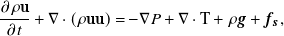 \begin{equation} \frac {\partial {{\rho \mathbf {u}}}}{\partial t} + { \nabla }\cdot ( {\rho \mathbf {u}\mathbf {u}} )= {{- \nabla {P}}} + {{\nabla }}\cdot {\textrm {T}}+ {{\rho \boldsymbol {g}}} + {{\boldsymbol {f_s}}}, \end{equation}
the continuity equation:
 \begin{equation} {\nabla }\cdot {\mathbf {u}} = 0 \end{equation}
and the equation for the advection of fluid fraction $\varphi$
:
$\varphi$
:
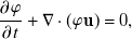 \begin{equation} \frac {\partial \varphi }{\partial t}+\nabla \cdot (\varphi \mathbf {u})=0, \end{equation}
where $\textbf {u}$
is the velocity vector field,
$\textbf {u}$
is the velocity vector field, $P$
is the pressure and
$P$
is the pressure and $T= 2 \eta E - 2 \eta (\nabla \cdot \mathbf {u}) I / 3$
is the deviatoric stress tensor with
$T= 2 \eta E - 2 \eta (\nabla \cdot \mathbf {u}) I / 3$
is the deviatoric stress tensor with $E$
as the rate of deformation tensor (the symmetric part of the velocity gradient tensor) and
$E$
as the rate of deformation tensor (the symmetric part of the velocity gradient tensor) and $I$
as the identity matrix. The fluid fraction
$I$
as the identity matrix. The fluid fraction $\varphi$
varies smoothly between 0 and 1, such that
$\varphi$
varies smoothly between 0 and 1, such that $\varphi = 0$
for the core fluid and
$\varphi = 0$
for the core fluid and $\varphi = 1$
for the sheath fluid. The body force per unit volume
$\varphi = 1$
for the sheath fluid. The body force per unit volume $\boldsymbol {f_s}$
is localised to the interface between the core and sheath fluids as defined below and accounts for the surface tension forces.
$\boldsymbol {f_s}$
is localised to the interface between the core and sheath fluids as defined below and accounts for the surface tension forces.
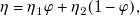
The bulk parameters density $\rho$
and viscosity
$\rho$
and viscosity $\eta$
are computed based on the weighted average distribution of the fluid fraction
$\eta$
are computed based on the weighted average distribution of the fluid fraction $\varphi$
:
$\varphi$
:
 \begin{align} \rho = \rho {_1} \varphi + {\rho _2} (1 - \varphi ), \end{align}
 \begin{align} \eta = \eta {_1} \varphi + {\eta _2} (1 - \varphi ), \\[8pt]\nonumber\end{align}
where $\rho _1$
,
$\rho _1$
, $\rho _2$
,
$\rho _2$
, $\eta _1$
,
$\eta _1$
, $\eta _2$
are the densities and the viscosities of the two fluids. The surface tension force
$\eta _2$
are the densities and the viscosities of the two fluids. The surface tension force $\boldsymbol {f_s}$
is modelled as a volumetric force using the continuum surface force method (Brackbill, Kothe & Zemach Reference Brackbill, Kothe and Zemach1992), and is defined as
$\boldsymbol {f_s}$
is modelled as a volumetric force using the continuum surface force method (Brackbill, Kothe & Zemach Reference Brackbill, Kothe and Zemach1992), and is defined as
 \begin{equation} {\boldsymbol {f_s}}=\gamma \kappa \nabla \varphi , \end{equation}
where $\varphi$
is the fluid fraction,
$\varphi$
is the fluid fraction, $\gamma$
the interfacial tension and
$\gamma$
the interfacial tension and $\kappa$
the local curvature of the interface determined by
$\kappa$
the local curvature of the interface determined by
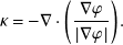 \begin{equation} {\kappa = -\nabla \cdot \left (\frac {\nabla \varphi }{|\nabla \varphi |}\right )}. \end{equation}
In addition to the complex rheology, the dynamics of the physical flow system is controlled by an ultralow EIT of $\mathcal {O} (10^{-4}-$ $10^{1})$
mN
$10^{1})$
mN $\,$
m
$\,$
m $^{-1}$
(Truzzolillo et al. Reference Truzzolillo, Roger, Dupas, Mora and Cipelletti2015, Reference Truzzolillo, Mora, Dupas and Cipelletti2016). As indicated by its name, the effect of the EIT resembles the effects of interfacial tension. The EIT models the Korteweg stresses (Korteweg Reference Korteweg1901) that appear due to the fibril concentration gradient between the CNF dispersion (core fluid) and its solvent (sheath fluid) (Atencia & Beebe Reference Atencia and Beebe2005; Joseph & Renardy Reference Joseph and Renardy1993). For the present combination of CNF dispersion–solvent fluid pair, an extensive comparison between experimental and numerical flow data (Gowda et al. Reference Gowda. V, Brouzet, Lefranc, Söderberg and Lundell2019) found that the flow modelling reproduces the experimental flow characteristics when
$^{-1}$
(Truzzolillo et al. Reference Truzzolillo, Roger, Dupas, Mora and Cipelletti2015, Reference Truzzolillo, Mora, Dupas and Cipelletti2016). As indicated by its name, the effect of the EIT resembles the effects of interfacial tension. The EIT models the Korteweg stresses (Korteweg Reference Korteweg1901) that appear due to the fibril concentration gradient between the CNF dispersion (core fluid) and its solvent (sheath fluid) (Atencia & Beebe Reference Atencia and Beebe2005; Joseph & Renardy Reference Joseph and Renardy1993). For the present combination of CNF dispersion–solvent fluid pair, an extensive comparison between experimental and numerical flow data (Gowda et al. Reference Gowda. V, Brouzet, Lefranc, Söderberg and Lundell2019) found that the flow modelling reproduces the experimental flow characteristics when $\gamma$
= 0.054 mN m
$\gamma$
= 0.054 mN m $^{-1}$
. The significance of EIT on the flow dynamics of miscible co-flowing fluids was further demonstrated recently by Carbonaro et al. (Reference Carbonaro, Savorana, Cipelletti, Govindarajan and Truzzolillo2025).
$^{-1}$
. The significance of EIT on the flow dynamics of miscible co-flowing fluids was further demonstrated recently by Carbonaro et al. (Reference Carbonaro, Savorana, Cipelletti, Govindarajan and Truzzolillo2025).
In our previous works (Gowda et al. Reference Gowda. V, Brouzet, Lefranc, Söderberg and Lundell2019; Gowda et al. Reference Gowda, Rydefalk, Söderberg and Lundell2021), we have thoroughly evaluated and demonstrated that the flow model described above reproduces the experimental flow features with very good agreement in terms of three-dimensional (3-D) flow topology and velocity fields as measured by optical coherence tomography.
2.2. Fibril orientation
The Smoluchowski equation (Hyensjö & Dahlkild Reference Hyensjö and Dahlkild2008) describing the evolution of the orientation distribution $\varPsi$
of monodisperse non-spherical particles is written as
$\varPsi$
of monodisperse non-spherical particles is written as
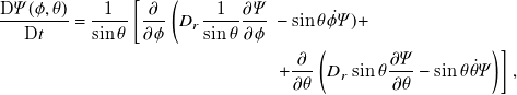 \begin{equation} \begin{aligned} \frac {\mathrm {D} \varPsi (\phi , \theta )}{\mathrm {D} t}=\frac {1}{\sin \theta }\left [\frac { \partial } { \partial \phi } \left (D_r \frac {1}{\sin \theta } \frac {\partial \varPsi }{\partial \phi }\right .\right . & -\sin \theta \dot {\phi } \varPsi )+ \\ & \left .+\frac {\partial }{\partial \theta }\left (D_r \sin \theta \frac {\partial \varPsi }{\partial \theta }-\sin \theta \dot {\theta } \varPsi \right )\right ], \end{aligned} \end{equation}
where $\mathrm {D} / \mathrm {D} t$
is the material derivative following the fluid,
$\mathrm {D} / \mathrm {D} t$
is the material derivative following the fluid, $D_r$
is the Brownian rotary diffusion coefficient and
$D_r$
is the Brownian rotary diffusion coefficient and $\dot \theta$
and
$\dot \theta$
and $\dot \phi$
are the rotational velocities of the particle based on the velocity gradients of the flow, the dot denoting temporal derivative. The rotational velocities are obtained from the rate of change of the director of a particle
$\dot \phi$
are the rotational velocities of the particle based on the velocity gradients of the flow, the dot denoting temporal derivative. The rotational velocities are obtained from the rate of change of the director of a particle $\textbf { p}$
, defined as
$\textbf { p}$
, defined as
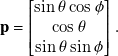 \begin{equation} \begin{aligned} \textbf { p} &= \begin{bmatrix} \sin \theta \cos \phi \\ \cos \theta \\ \sin \theta \sin \phi \end{bmatrix}. \end{aligned} \end{equation}
Assuming ellipsoidal particles and the flow to be very viscous (Stokes), the rate of change of $\textbf { p}$
(Doi & Edwards Reference Doi and Edwards1988; Jeffery Reference Jeffery1922) in the local flow field is given by
$\textbf { p}$
(Doi & Edwards Reference Doi and Edwards1988; Jeffery Reference Jeffery1922) in the local flow field is given by
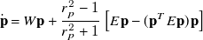 \begin{equation} \dot {\textbf { p}}= { W \textbf p} + \frac {r_p^2-1}{r_p^2+1}\left [{E \textbf p} - (\textbf{p}^T{E \textbf p})\textbf {p}\right ] \end{equation}
via a projection on the unit vectors of the spherical coordinates, i.e.
 \begin{equation} \dot \phi = \dot {\textbf { p}} \cdot {\textbf { e}}_\phi , \quad \dot \theta = \dot {\textbf { p}} \cdot {\textbf { e}}_\theta , \end{equation}
where $E$
and
$E$
and $W$
are the symmetric (rate of deformation) and antisymmetric (vorticity) parts of the velocity gradient tensor obtained from flow modelling. The parameter
$W$
are the symmetric (rate of deformation) and antisymmetric (vorticity) parts of the velocity gradient tensor obtained from flow modelling. The parameter $r_p$
is the aspect ratio of the particle;
$r_p$
is the aspect ratio of the particle; $r_p\gt 1$
for prolate (cucumber-like) and
$r_p\gt 1$
for prolate (cucumber-like) and $r_p\lt 1$
for oblate (pancake-like) particles. For the fibrils in the present work,
$r_p\lt 1$
for oblate (pancake-like) particles. For the fibrils in the present work, $r_p\gt 25$
and
$r_p\gt 25$
and $(r_p^2-1)/(r_p^2+1)\approx 1$
. Equations (2.11)–(2.12) describe the coupling between particle rotation and velocity gradients of flow assuming that the particles are stiff and straight rod-like.
$(r_p^2-1)/(r_p^2+1)\approx 1$
. Equations (2.11)–(2.12) describe the coupling between particle rotation and velocity gradients of flow assuming that the particles are stiff and straight rod-like.
Illustration of evolution of 3-D nanofibril orientation distribution $\varPsi$
along the channel length at different downstream
$\varPsi$
along the channel length at different downstream $x/h$
positions. The mean order parameter
$x/h$
positions. The mean order parameter $S$
and the projected order parameter
$S$
and the projected order parameter $S_{\textrm {proj}}$
are obtained from the average of cross-sectional local order
$S_{\textrm {proj}}$
are obtained from the average of cross-sectional local order $S_{\textrm {local}}$
(equation (2.13)) and projected orientation (equation (2.14)) distributions, respectively.
$S_{\textrm {local}}$
(equation (2.13)) and projected orientation (equation (2.14)) distributions, respectively.
Further, the 3-D orientation distributions $\varPsi$
of the particles can be quantified through a variable called the mean order parameter
$\varPsi$
of the particles can be quantified through a variable called the mean order parameter $S$
, where
$S$
, where $S=1$
represents an anisotropic distribution and
$S=1$
represents an anisotropic distribution and $S = 0$
corresponds to isotropic distribution, i.e. random orientation. The order parameter can be evaluated in two ways as illustrated schematically in figure 3. The first is by calculating the local order parameter
$S = 0$
corresponds to isotropic distribution, i.e. random orientation. The order parameter can be evaluated in two ways as illustrated schematically in figure 3. The first is by calculating the local order parameter $S_{\textrm {local}}$
as (Doi & Edwards Reference Doi and Edwards1988)
$S_{\textrm {local}}$
as (Doi & Edwards Reference Doi and Edwards1988)
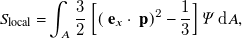 \begin{equation} S_{\textrm {local}} = \int _A\frac {3}{2}\left [\left (\textbf { e}_x \cdot \textbf { p}\right )^2-\frac {1} {3}\right ]\varPsi\, \mathrm {d}A, \end{equation}
where $\textbf { e}_x$
is the unit vector in the streamwise
$\textbf { e}_x$
is the unit vector in the streamwise $x$
direction and the integration is made over the unit sphere. The mean order parameter
$x$
direction and the integration is made over the unit sphere. The mean order parameter $S$
is the average of the local order parameter
$S$
is the average of the local order parameter $S_{\textrm {local}}$
over the cross-section. The second is the projected order parameter
$S_{\textrm {local}}$
over the cross-section. The second is the projected order parameter $S_{\textrm {proj}}$
based on the projected mean orientation distribution
$S_{\textrm {proj}}$
based on the projected mean orientation distribution $\varPsi _{\textrm {proj}}(\chi )$
and is calculated as
$\varPsi _{\textrm {proj}}(\chi )$
and is calculated as
 \begin{equation} S_{\textrm {proj}}=\int _0^\pi \varPsi _{\textrm {proj}}(\chi )\left (\frac {3}{2}\cos ^2\chi -\frac {1}{2}\right )\sin \chi \,\mathrm {d}\chi , \end{equation}
where $\varPsi _{\textrm {proj}}$
is normalised according to
$\varPsi _{\textrm {proj}}$
is normalised according to
 \begin{equation} \int ^\pi _{0} \varPsi _{\textrm {proj}}(\chi )\sin \chi \,\mathrm {d}\chi = 1. \end{equation}
Note that $-0.5 \leq S_{\textrm {proj}} \leq 1$
, where the low and high extremes indicate that all fibrils are oriented normal and parallel to the flow direction, respectively.
$-0.5 \leq S_{\textrm {proj}} \leq 1$
, where the low and high extremes indicate that all fibrils are oriented normal and parallel to the flow direction, respectively.
The total variation of the local order parameter ( $S_{\textrm {local}}$
) over the cross-section is measured by the standard deviation at each streamwise position and is denoted as
$S_{\textrm {local}}$
) over the cross-section is measured by the standard deviation at each streamwise position and is denoted as $\Delta S$
.
$\Delta S$
.
Using the numerical method and two-fraction model described in Gowda et al. (Reference Gowda, Rosén, Roth, Söderberg and Lundell2022), the Smoluchowski equation (equation (2.9)) for the 3-D orientation distribution $\varPsi$
is solved along streamlines as depicted in figure 3. The Smoluchowski equation uses the flow gradients from flow modelling (see figure 2
a) as an input together with rotary diffusion(s)
$\varPsi$
is solved along streamlines as depicted in figure 3. The Smoluchowski equation uses the flow gradients from flow modelling (see figure 2
a) as an input together with rotary diffusion(s) $D_r$
. In previous work on CNF alignment in flows (Gowda et al. Reference Gowda, Rosén, Roth, Söderberg and Lundell2022), it was found that a two-fraction model, where one fraction (
$D_r$
. In previous work on CNF alignment in flows (Gowda et al. Reference Gowda, Rosén, Roth, Söderberg and Lundell2022), it was found that a two-fraction model, where one fraction ( $\alpha _{\textrm {fast}}$
) of the dispersion was assumed to have a high
$\alpha _{\textrm {fast}}$
) of the dispersion was assumed to have a high $D_{r,\textrm {fast}}$
and the other
$D_{r,\textrm {fast}}$
and the other $(1 - \alpha _{\textrm {fast}})$
a low
$(1 - \alpha _{\textrm {fast}})$
a low $D_{r,\textrm {slow}}$
, could reproduce the projected order parameter
$D_{r,\textrm {slow}}$
, could reproduce the projected order parameter $S_{\textrm {proj}}$
(see below) obtained from SAXS measurements.
$S_{\textrm {proj}}$
(see below) obtained from SAXS measurements.
As mentioned in the introduction, the two-fraction model is a coarse approximation of the actual continuous distribution originating from the length distribution of the fibrils (Brouzet et al. Reference Brouzet, Mittal, Söderberg and Lundell2018). In the present context, increasing the number of fractions above two does not add to the prediction accuracy. Furthermore, with more than two fractions, the objective function (integrated difference between measured and modelled projected order parameter) does not have a distinct minimum and unique values of model parameters are not obtained.
2.3. Cellulose nanofibril dispersion
The core fluid is a 0.3 % by weight dispersion of CNFs in water. The fibrils have a diameter ranging from 2 to 6 nm, and a length distribution ranging from 100 to 1500 nm. This kind of dispersion is of special interest since it has been used to assemble and fabricate very strong cellulose filaments (Håkansson et al. Reference Håkansson, Fall, Lundell, Yu, Krywka, Roth, Santoro, Kvick, Prahl Wittberg, Wågberg and Söderberg2014; Mittal et al. Reference Mittal, Ansari, Gowda, Brouzet, Chen, Larsson, Roth, Lundell, Wågberg, Kotov and Söderberg2018). The rheological characterisation of the dispersion was performed with steady shear viscosity measurements. As seen from figure 2 b, the dispersion displays a shear-thinning rheological behaviour, described by the non-Newtonian Carreau model (equation (2.1)).
2.4. Small-angle X-ray scattering
The fibril orientation in the flow-focusing configurations is quantified experimentally through SAXS measurements. The SAXS experiments were performed at the P03 beamline (Buffet et al. Reference Buffet, Rothkirch, Döhrmann, Körstgens, Abul Kashem, Perlich, Herzog, Schwartzkopf, Gehrke, Müller-Buschbaum and Roth2012) of the PETRA III Synchrotron facility at Deutsches Elektronen-Synchrotron (DESY) in Hamburg, Germany.
An X-ray beam of size 24 μm $\times$
11 μm having a wavelength
$\times$
11 μm having a wavelength $\lambda = 0.95$
Å traverses the flow-focusing channel in
$\lambda = 0.95$
Å traverses the flow-focusing channel in $x$
and
$x$
and $y$
directions, as illustrated pictorially in figure 2
c. The X-ray intensity scattered by the flowing colloidal fibril dispersion is recorded on the detector (Pilatus 1M, Dectris, having a pixel size of 172 μm
$y$
directions, as illustrated pictorially in figure 2
c. The X-ray intensity scattered by the flowing colloidal fibril dispersion is recorded on the detector (Pilatus 1M, Dectris, having a pixel size of 172 μm $\times$
172 μm), positioned at a distance of
$\times$
172 μm), positioned at a distance of $L_d =$
7.5 m from the flow-focusing channel assembly. The magnitude of the scattering vector
$L_d =$
7.5 m from the flow-focusing channel assembly. The magnitude of the scattering vector $q$
is given by
$q$
is given by $ q = (4 \pi / \lambda ) \sin \kappa$
. The angle between incident and scattered light is
$ q = (4 \pi / \lambda ) \sin \kappa$
. The angle between incident and scattered light is $2 \kappa$
(see figure 2
c). The background scattering intensities were removed using scattering intensities obtained with the scans of deionised water.
$2 \kappa$
(see figure 2
c). The background scattering intensities were removed using scattering intensities obtained with the scans of deionised water.
The orientation distribution $\varPsi$
of the nanofibrils in the scattered SAXS diffractograms is quantified with order parameter
$\varPsi$
of the nanofibrils in the scattered SAXS diffractograms is quantified with order parameter $S$
(Van Gurp Reference Van Gurp1995) written as
$S$
(Van Gurp Reference Van Gurp1995) written as
 \begin{equation} S= \left \langle \frac {3}{2}\cos ^2\chi -\frac {1}{2}\right \rangle , \end{equation}
where $ \langle \cdot \rangle$
indicates an ensemble average of the particles. If all the nanofibrils are aligned with the flow direction, the order parameter
$ \langle \cdot \rangle$
indicates an ensemble average of the particles. If all the nanofibrils are aligned with the flow direction, the order parameter $S = 1$
. For an isotropic distribution, i.e. random orientation,
$S = 1$
. For an isotropic distribution, i.e. random orientation, $S = 0$
. Further, as seen from figure 2
c, the SAXS pattern captured by the two-dimensional detector along the beam path represents the projected mean orientation distribution
$S = 0$
. Further, as seen from figure 2
c, the SAXS pattern captured by the two-dimensional detector along the beam path represents the projected mean orientation distribution $\varPsi _{\textrm {proj}}(\chi )$
, and the projected order parameter
$\varPsi _{\textrm {proj}}(\chi )$
, and the projected order parameter $S_{\textrm {proj}}$
is obtained according to equations (2.14) and (2.15).
$S_{\textrm {proj}}$
is obtained according to equations (2.14) and (2.15).
3. Results and discussion
3.1. Effect of confluence angle
3.1.1. Flow topology and flow fields
The flow in all confluence angles $\beta$
from 30
$\beta$
from 30 $^\circ$
to 150
$^\circ$
to 150 $^\circ$
(see figure 1
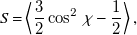
a–e) was studied numerically and experimentally by Gowda et al. (Reference Gowda, Rydefalk, Söderberg and Lundell2021). The agreement between numerical and experimental results was excellent. In figure 4, the results are summarised in terms of aspect ratio
$^\circ$
(see figure 1
a–e) was studied numerically and experimentally by Gowda et al. (Reference Gowda, Rydefalk, Söderberg and Lundell2021). The agreement between numerical and experimental results was excellent. In figure 4, the results are summarised in terms of aspect ratio $\epsilon _z/\epsilon _y$
of the core fluid thread, where
$\epsilon _z/\epsilon _y$
of the core fluid thread, where $\epsilon _y$
and
$\epsilon _y$
and $\epsilon _z$
are the dimensions of the thread in the
$\epsilon _z$
are the dimensions of the thread in the $y$
and
$y$
and $z$
directions, respectively, and acceleration (strain rate
$z$
directions, respectively, and acceleration (strain rate $\dot {\varepsilon }$
) as a function of downstream
$\dot {\varepsilon }$
) as a function of downstream $x/h$
positions, as well as maximum
$x/h$
positions, as well as maximum $Ar_{\textrm {max}}$
and final
$Ar_{\textrm {max}}$
and final $Ar_{\textrm {final}}$
thread aspect ratio. As the confluence angle
$Ar_{\textrm {final}}$
thread aspect ratio. As the confluence angle $\beta$
deviates from 90
$\beta$
deviates from 90 $^\circ$
, the aspect ratio decreases towards a circular cross-section and the acceleration increases. A somewhat surprising observation is that the results, to a large extent, are symmetric so that the aspect ratio development and flow acceleration are very similar for each of the two pairs
$^\circ$
, the aspect ratio decreases towards a circular cross-section and the acceleration increases. A somewhat surprising observation is that the results, to a large extent, are symmetric so that the aspect ratio development and flow acceleration are very similar for each of the two pairs $\beta$
= (60
$\beta$
= (60 $^\circ$
, 120
$^\circ$
, 120 $^\circ$
) and
$^\circ$
) and $\beta$
= (30
$\beta$
= (30 $^\circ$
, 150
$^\circ$
, 150 $^\circ$
).
$^\circ$
).
(a) Development of thread aspect ratio ( $\epsilon _z/\epsilon _y$
) as a function of downstream
$\epsilon _z/\epsilon _y$
) as a function of downstream $x/h$
positions for different confluence angle
$x/h$
positions for different confluence angle $\beta$
geometries. (b) Maximum (
$\beta$
geometries. (b) Maximum ( $Ar_{\textrm {max}}$
,open
$Ar_{\textrm {max}}$
,open![]() symbols) and final (
symbols) and final ( $Ar_{\textrm {final}}$
,filled
$Ar_{\textrm {final}}$
,filled![]() symbols) thread aspect ratio versus the confluence angle
symbols) thread aspect ratio versus the confluence angle $\beta$
. (c) Evolution of strain rate
$\beta$
. (c) Evolution of strain rate $\dot {\varepsilon }$
along the centreline as a function of downstream positions
$\dot {\varepsilon }$
along the centreline as a function of downstream positions $x/h$
for different geometries.
$x/h$
for different geometries.
3.1.2. Fibril alignment: comparison between experiments and simulations
(a–c) Comparison of simulated (Num.) and measured (Exp.) fibril order ( $S_{\textrm {proj}}$
) as a function of downstream
$S_{\textrm {proj}}$
) as a function of downstream $x/h$
positions for three confluence angle (
$x/h$
positions for three confluence angle ( $\beta = 90^\circ , 60^\circ$
and
$\beta = 90^\circ , 60^\circ$
and $120^\circ$
) geometries. The experimental order parameter is obtained from SAXS measurements, while the simulations are based on equations (2.9)–(2.12) with a two-fraction model. Care is taken to extract the measured quantity (space averaged and projected order parameter) from the simulated data.
$120^\circ$
) geometries. The experimental order parameter is obtained from SAXS measurements, while the simulations are based on equations (2.9)–(2.12) with a two-fraction model. Care is taken to extract the measured quantity (space averaged and projected order parameter) from the simulated data.
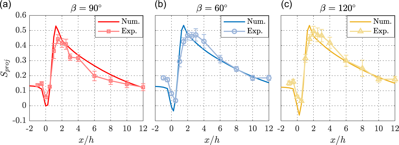
First, the comparisons between alignment simulations and experiments are extended from the confluence angle $\beta =$
90
$\beta =$
90 $^\circ$
studied by Gowda et al. (Reference Gowda, Rosén, Roth, Söderberg and Lundell2022) to
$^\circ$
studied by Gowda et al. (Reference Gowda, Rosén, Roth, Söderberg and Lundell2022) to $\beta =$
60
$\beta =$
60 $^\circ$
and 120
$^\circ$
and 120 $^\circ$
geometries, as shown in figure 5(a–c). The experimental order parameters from SAXS measurements were deduced using two datasets in the case of
$^\circ$
geometries, as shown in figure 5(a–c). The experimental order parameters from SAXS measurements were deduced using two datasets in the case of $\beta$
= 90
$\beta$
= 90 $^\circ$
, and one each from
$^\circ$
, and one each from $\beta$
= 60
$\beta$
= 60 $^\circ$
and
$^\circ$
and $\beta$
= 120
$\beta$
= 120 $^\circ$
. In all cases, the projected order parameter
$^\circ$
. In all cases, the projected order parameter $S_{\textrm {proj}}$
, where
$S_{\textrm {proj}}$
, where $S_{\textrm {proj}} = 1$
means that all fibrils are aligned in the flow direction,
$S_{\textrm {proj}} = 1$
means that all fibrils are aligned in the flow direction, $S_{\textrm {proj}}=0$
is an isotropic system and
$S_{\textrm {proj}}=0$
is an isotropic system and $S_{\textrm {proj}}=-0.5$
is a system where all fibrils are aligned normal to the flow direction, shows the same general behaviour: a slight alignment (
$S_{\textrm {proj}}=-0.5$
is a system where all fibrils are aligned normal to the flow direction, shows the same general behaviour: a slight alignment ( $0.12 \lt S_{\textrm {proj}} \lt 0.2$
) for
$0.12 \lt S_{\textrm {proj}} \lt 0.2$
) for $x/h \lt 0$
, i.e. in the inlet core flow channel. In the confluence region
$x/h \lt 0$
, i.e. in the inlet core flow channel. In the confluence region $0\lt x/h\lt 1$
, there is first a decrease of alignment followed by a rapid increase to a maximum around 0.5 slightly before and after
$0\lt x/h\lt 1$
, there is first a decrease of alignment followed by a rapid increase to a maximum around 0.5 slightly before and after $x/h=2$
for the
$x/h=2$
for the $\beta =$
90
$\beta =$
90 $^\circ$
case (figure 5
a) and
$^\circ$
case (figure 5
a) and $\beta =$
(60
$\beta =$
(60 $^\circ$
,120
$^\circ$
,120 $^\circ$
) cases (figure 5
b,c), respectively. The numerical alignment model is seen to capture the general behaviour very well, but the full difference between the experimental data in figure 5(a) as compared with figure 5(b,c) is not captured: the simulated curves tend to be above the experiments in figure 5(a) and below in figure 5(b,c). Nevertheless, the simulated alignment captures the experimental observations, including the subtle variations between the different confluence angles, fairly well.
$^\circ$
) cases (figure 5
b,c), respectively. The numerical alignment model is seen to capture the general behaviour very well, but the full difference between the experimental data in figure 5(a) as compared with figure 5(b,c) is not captured: the simulated curves tend to be above the experiments in figure 5(a) and below in figure 5(b,c). Nevertheless, the simulated alignment captures the experimental observations, including the subtle variations between the different confluence angles, fairly well.
The calibrated alignment model of figure 5 is used to investigate the fibril alignment in the remainder of the paper. It differs somewhat from the model used in Gowda et al. (Reference Gowda, Rosén, Roth, Söderberg and Lundell2022). After fitting the model to all three confluence angle ( $\beta = 90^\circ , 60^\circ$
and
$\beta = 90^\circ , 60^\circ$
and $120^\circ$
) geometries, the parameters
$120^\circ$
) geometries, the parameters $D_{r,\textrm {slow}}=\,0.45$
s
$D_{r,\textrm {slow}}=\,0.45$
s $^{-1}$
,
$^{-1}$
, $D_{r,\textrm {fast}}=6.4$
s
$D_{r,\textrm {fast}}=6.4$
s $^{-1}$
and
$^{-1}$
and $\alpha _{\textrm {fast}}=0.74$
are found to be optimal (i.e. the mean of root-mean-square error is reduced from 0.055 to 0.047 as compared with the parameter values used in Gowda et al. (Reference Gowda, Rosén, Roth, Söderberg and Lundell2022)).
$\alpha _{\textrm {fast}}=0.74$
are found to be optimal (i.e. the mean of root-mean-square error is reduced from 0.055 to 0.047 as compared with the parameter values used in Gowda et al. (Reference Gowda, Rosén, Roth, Söderberg and Lundell2022)).
3.1.3. Fibril alignment in a wider range of confluence angle geometries
Having seen the two-fraction model capturing the experimental observations of fibril alignment quite well in all the three channel configurations ( $\beta = 90^\circ , 60^\circ$
and
$\beta = 90^\circ , 60^\circ$
and $120^\circ$
), we now utilise the two-fraction model to understand the 3-D fibril orientation states for a wider range of confluence angles (see figure 1
a–e). In particular, it is shown how the acceleration shown in figure 4
c affects fibril orientation.
$120^\circ$
), we now utilise the two-fraction model to understand the 3-D fibril orientation states for a wider range of confluence angles (see figure 1
a–e). In particular, it is shown how the acceleration shown in figure 4
c affects fibril orientation.
Streamwise development of mean order parameter $S$
(a),
$S$
(a), $\Delta S$
(b) and
$\Delta S$
(b) and $S/ \Delta S$
(c) as a function of downstream
$S/ \Delta S$
(c) as a function of downstream $x/h$
positions for different confluence angle
$x/h$
positions for different confluence angle $\beta$
geometries. The confluence angle
$\beta$
geometries. The confluence angle $\beta$
of each geometrical configuration is indicated in the legend (b). The black square
$\beta$
of each geometrical configuration is indicated in the legend (b). The black square![]() symbols on the horizontal axis in (a) correspond to the streamwise
symbols on the horizontal axis in (a) correspond to the streamwise $x/h$
positions of the cross-sectional contours depicted in (e,f). (d–f) Cross-sectional contours of local order parameter
$x/h$
positions of the cross-sectional contours depicted in (e,f). (d–f) Cross-sectional contours of local order parameter $S_{\textrm {local}}$
, at different streamwise
$S_{\textrm {local}}$
, at different streamwise $x/h$
positions. In (e,f), each quarter segment represents different geometrical configurations, and the confluence angle
$x/h$
positions. In (e,f), each quarter segment represents different geometrical configurations, and the confluence angle $\beta$
of each configuration is indicated in (d).
$\beta$
of each configuration is indicated in (d).
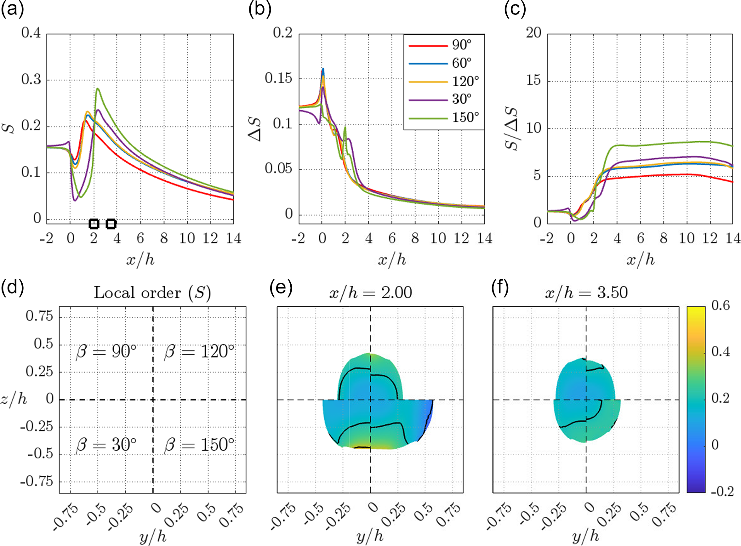
Accordingly, figure 6 shows the quantitative evolution of mean order parameter $S$
,
$S$
, $\Delta S$
and
$\Delta S$
and $S/\Delta S$
over the cross-sections as a function of downstream
$S/\Delta S$
over the cross-sections as a function of downstream $x/h$
positions for different confluence angles
$x/h$
positions for different confluence angles $\beta$
. The black squares
$\beta$
. The black squares![]() on the horizontal axis indicate the streamwise positions of the cross-sectional contours plotted in figure 6(e,f). From the mean order
on the horizontal axis indicate the streamwise positions of the cross-sectional contours plotted in figure 6(e,f). From the mean order $S$
in figure 6(a), for
$S$
in figure 6(a), for $x/h \leq 0$
,
$x/h \leq 0$
, $S$
is almost constant at
$S$
is almost constant at $0.16$
in all cases. At the start of the confluence junction (
$0.16$
in all cases. At the start of the confluence junction ( $x/h \gt 0$
), i.e. right at the entry of the sheath flows, there is a decrease in
$x/h \gt 0$
), i.e. right at the entry of the sheath flows, there is a decrease in $S$
for all the configurations as seen from the order distributions in figure 6(a) (
$S$
for all the configurations as seen from the order distributions in figure 6(a) ( $x/h = 0.5$
). In the
$x/h = 0.5$
). In the $\beta = 30 ^\circ$
and
$\beta = 30 ^\circ$
and $ \beta = 150 ^\circ$
geometries, the decrease in
$ \beta = 150 ^\circ$
geometries, the decrease in $S$
for 0
$S$
for 0 $\leq$ $x/h$
$x/h$ $\leq$
1.5 is larger compared with the other configurations (
$\leq$
1.5 is larger compared with the other configurations ( $\beta = 90 ^\circ , 60^\circ$
and
$\beta = 90 ^\circ , 60^\circ$
and $120 ^\circ$
), since the deceleration is larger in the two former cases (see figure 4
c).
$120 ^\circ$
), since the deceleration is larger in the two former cases (see figure 4
c).
Further, after $x/h\gt 1.00$
, as depicted in figure 6(a) (
$x/h\gt 1.00$
, as depicted in figure 6(a) ( $x/h = 1.50, 3.00$
), the order continues to increase due to acceleration of the core fluid dispersion generated by the sheath flows, in turn leading to the alignment of fibrils. The highest order of fibril alignment varies among the configurations. As can be seen from the mean order in figure 6(a), the peak order for
$x/h = 1.50, 3.00$
), the order continues to increase due to acceleration of the core fluid dispersion generated by the sheath flows, in turn leading to the alignment of fibrils. The highest order of fibril alignment varies among the configurations. As can be seen from the mean order in figure 6(a), the peak order for $\beta = (60^\circ , 120 ^\circ$
) and
$\beta = (60^\circ , 120 ^\circ$
) and $\beta = (30^\circ , 150 ^\circ$
) cases occurs around
$\beta = (30^\circ , 150 ^\circ$
) cases occurs around $x/h \simeq 2$
and
$x/h \simeq 2$
and $x/h \simeq 2.5$
, respectively. Far downstream,
$x/h \simeq 2.5$
, respectively. Far downstream, $x/h \gt 3.00$
, the order decays for all cases. It is worth noting that the
$x/h \gt 3.00$
, the order decays for all cases. It is worth noting that the $\beta = 150 ^\circ$
flow-focusing configuration has higher order and a slower decay far downstream (
$\beta = 150 ^\circ$
flow-focusing configuration has higher order and a slower decay far downstream ( $x/h \gt 3$
), whereas the standard
$x/h \gt 3$
), whereas the standard $\beta = 90 ^\circ$
flow-focusing configuration has lower maximum order and a more upstream start of the decay (
$\beta = 90 ^\circ$
flow-focusing configuration has lower maximum order and a more upstream start of the decay ( $x/h \gt 1.75$
).
$x/h \gt 1.75$
).
Another important aspect to note from figure 6(a) is on the collapse of mean order on top of each other between $\beta = 60 ^\circ$
and
$\beta = 60 ^\circ$
and $ \beta = 120 ^\circ$
geometries. The resemblance between these two cases was also seen earlier in the evolution of thread shapes (see figure 4
a) and strain rate
$ \beta = 120 ^\circ$
geometries. The resemblance between these two cases was also seen earlier in the evolution of thread shapes (see figure 4
a) and strain rate $\dot {\varepsilon }$
along the centreline (see figure 4
c). On the other hand, the asymmetric behaviour between
$\dot {\varepsilon }$
along the centreline (see figure 4
c). On the other hand, the asymmetric behaviour between $\beta = 30 ^\circ$
and
$\beta = 30 ^\circ$
and $ \beta = 150 ^\circ$
cases (see figure 4
a,c) is also reflected in the mean order. Also, as seen from figure 6(c),
$ \beta = 150 ^\circ$
cases (see figure 4
a,c) is also reflected in the mean order. Also, as seen from figure 6(c), $S/\Delta S$
, i.e. ratio of alignment to its variation over the cross-section, is smallest for
$S/\Delta S$
, i.e. ratio of alignment to its variation over the cross-section, is smallest for $\beta = 90^\circ$
, and the other geometries have a higher degree of alignment and less variation.
$\beta = 90^\circ$
, and the other geometries have a higher degree of alignment and less variation.
Further, figure 6(e,f) shows the cross-sectional contours of local order at different streamwise $x/h$
positions. In all the flow-focusing configurations, the symmetry along
$x/h$
positions. In all the flow-focusing configurations, the symmetry along $xy$
and
$xy$
and $xz$
planes is exploited, and hence only a quarter of their cross-section is shown. Thus, in figure 6(e,f), each quarter segment represents a different geometrical configuration, and the confluence angles
$xz$
planes is exploited, and hence only a quarter of their cross-section is shown. Thus, in figure 6(e,f), each quarter segment represents a different geometrical configuration, and the confluence angles $\beta$
are given in figure 6(d). As seen from figure 6(e,f), all the configurations show an increase in the local order parameter towards the edge of the thread. This increased alignment originates from the regions close to the walls of the inlet channel, where the fibril dispersion is exposed to direct shear. This can be noted more clearly from figure 6(e) at
$\beta$
are given in figure 6(d). As seen from figure 6(e,f), all the configurations show an increase in the local order parameter towards the edge of the thread. This increased alignment originates from the regions close to the walls of the inlet channel, where the fibril dispersion is exposed to direct shear. This can be noted more clearly from figure 6(e) at $x/h = 2.00$
.
$x/h = 2.00$
.
3.2. Numerical evaluation of additional geometries
3.2.1. Description of the geometries
Illustration of top and cross-sectional views of flow-focusing configurations: (a) RC; (b,c) AR-1 to AR-4; (d,e) CC-1 to CC-4. The cross-sectional width $b$
and height
$b$
and height $h$
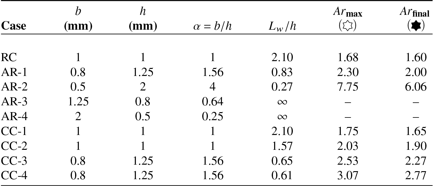
of all the geometrical configurations are tabulated in table 1.
$h$
of all the geometrical configurations are tabulated in table 1.
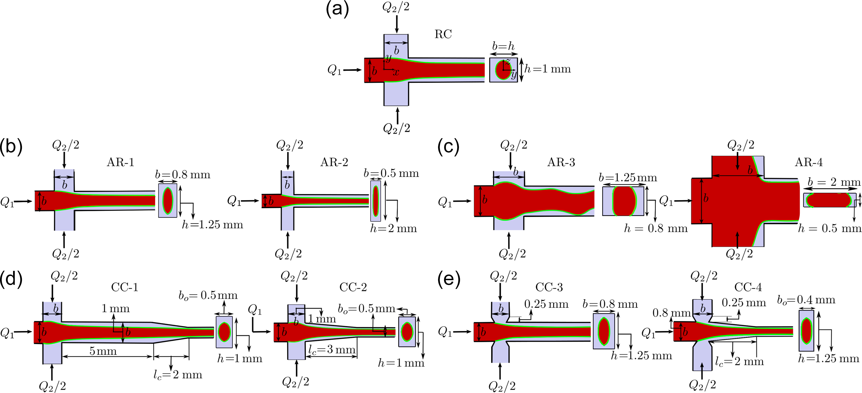
Figure 7 shows a schematic illustration of the top and cross-sectional views of the flow-focusing configurations. In total, nine geometrical configurations are investigated. The reference configuration (RC; figure 7
a) is a channel geometry of confluence angle $\beta = 90^\circ$
with square cross-section of sidelength
$\beta = 90^\circ$
with square cross-section of sidelength $h = 1$
mm. All the configurations have four channel arms: one main central channel arm for the core flow inlet, two side-channel arms for the sheath flow inlets and a central outlet channel arm. The channel cross-sectional aspect ratio is defined as
$h = 1$
mm. All the configurations have four channel arms: one main central channel arm for the core flow inlet, two side-channel arms for the sheath flow inlets and a central outlet channel arm. The channel cross-sectional aspect ratio is defined as $\alpha$
=
$\alpha$
= $b/h$
, where
$b/h$
, where $b$
and
$b$
and $h$
are the width and height of the channel arms, respectively.
$h$
are the width and height of the channel arms, respectively.
As seen from figures 7(a–c) and 8(a–c), the RC and AR-1 to AR-4 configurations have uniform cross-sections with the dimensions of width $b$
and height
$b$
and height $h$
as displayed in table 1. The cross-sectional area (
$h$
as displayed in table 1. The cross-sectional area ( $b\times h$
) of these configurations remains constant (1 mm
$b\times h$
) of these configurations remains constant (1 mm $^2$
), whereas the cross-sectional aspect ratio
$^2$
), whereas the cross-sectional aspect ratio $\alpha$
varies.
$\alpha$
varies.
In the cases of CC-1 to CC-4 (figures 7
d,e and 8
d,e), converging sections of varying lengths ( $ l_{c}$
= 0.25, 2 and 3 mm) are appended after the flow-focusing geometries. All the channel arms of the respective geometries have uniform height
$ l_{c}$
= 0.25, 2 and 3 mm) are appended after the flow-focusing geometries. All the channel arms of the respective geometries have uniform height $h$
as tabulated in table 1. When it comes to the width
$h$
as tabulated in table 1. When it comes to the width $b$
of the channel arms, only the width of the inlet channel arms is uniform, whereas the width
$b$
of the channel arms, only the width of the inlet channel arms is uniform, whereas the width $b_{o}$
of the outlet channel arms varies as shown in figure 7(d,e). The cross-sectional width
$b_{o}$
of the outlet channel arms varies as shown in figure 7(d,e). The cross-sectional width $b$
, height
$b$
, height $h$
and aspect ratio
$h$
and aspect ratio $\alpha$
of the inlet channel arms for all the configurations are reported in table 1.
$\alpha$
of the inlet channel arms for all the configurations are reported in table 1.
Further, in the CC-1 case, a converging section of length $ l_{c}$
= 2 mm starts at
$ l_{c}$
= 2 mm starts at $x/h=5$
, while, in the CC-2 case, a converging section of length
$x/h=5$
, while, in the CC-2 case, a converging section of length $ l_{c}$
= 3 mm begins right at the end of focusing region at
$ l_{c}$
= 3 mm begins right at the end of focusing region at $x/h = 1$
. In both CC-1 and CC-2 cases, the cross-sectional width
$x/h = 1$
. In both CC-1 and CC-2 cases, the cross-sectional width $b$
and height
$b$
and height $h$
of the inlet channel arms are the same as those of the RC case.
$h$
of the inlet channel arms are the same as those of the RC case.
For the CC-3 and CC-4 configurations, the cross-sectional width $b$
and height
$b$
and height $h$
of the inlet channel arms are equivalent to those of the AR-1 case. In both the CC-3 and CC-4 cases, the sheath flow inlet channel arms in the
$h$
of the inlet channel arms are equivalent to those of the AR-1 case. In both the CC-3 and CC-4 cases, the sheath flow inlet channel arms in the $y$
direction have a converging section of length
$y$
direction have a converging section of length $ l_{c}$
= 0.25 mm (figure 7
e) at the confluence region. In addition, for the CC-4 configuration, a converging section of length
$ l_{c}$
= 0.25 mm (figure 7
e) at the confluence region. In addition, for the CC-4 configuration, a converging section of length $ l_{c}$
= 2 mm is added in the streamwise
$ l_{c}$
= 2 mm is added in the streamwise $x$
direction right at the end (
$x$
direction right at the end ( $x/h = 1$
) of the focusing region.
$x/h = 1$
) of the focusing region.
Cross-sectional width $b$
, height
$b$
, height $h$
and aspect ratio
$h$
and aspect ratio $\alpha$
of the flow-focusing geometries illustrated in figure 7. The inlet channel of all the geometries has the same cross-sectional area
$\alpha$
of the flow-focusing geometries illustrated in figure 7. The inlet channel of all the geometries has the same cross-sectional area $b \times h$
= 1 mm
$b \times h$
= 1 mm $^2$
. The details of the thread features, namely the wetted length
$^2$
. The details of the thread features, namely the wetted length $L_{w}/h$
, thread aspect ratio
$L_{w}/h$
, thread aspect ratio $\varepsilon _{z}/\varepsilon _{y}$
, maximum
$\varepsilon _{z}/\varepsilon _{y}$
, maximum $Ar_{\textrm {max}}$
and final
$Ar_{\textrm {max}}$
and final $Ar_{\textrm {final}}$
, displayed in figures 9 and 10 are also tabulated.
$Ar_{\textrm {final}}$
, displayed in figures 9 and 10 are also tabulated.
Three-dimensional views of the thread shapes in various flow-focusing geometries: (a) RC; (b,c) AR-1 to AR-4; (d,e) CC-1 to CC- 4. The aqua colour zone at the top plane in all the geometries indicates the region wetted by the core fluid dispersion before detachment. In (c), the aqua colour extends all along the channel length in the $x$
direction indicating the core fluid dispersion never detaches from the top and bottom channel walls. The dashed magenta vertical lines along the centre of side channels in the
$x$
direction indicating the core fluid dispersion never detaches from the top and bottom channel walls. The dashed magenta vertical lines along the centre of side channels in the $z$
direction denote the upstream and downstream
$z$
direction denote the upstream and downstream $y/h$
positions of the velocity profiles plotted in figure 9.
$y/h$
positions of the velocity profiles plotted in figure 9.
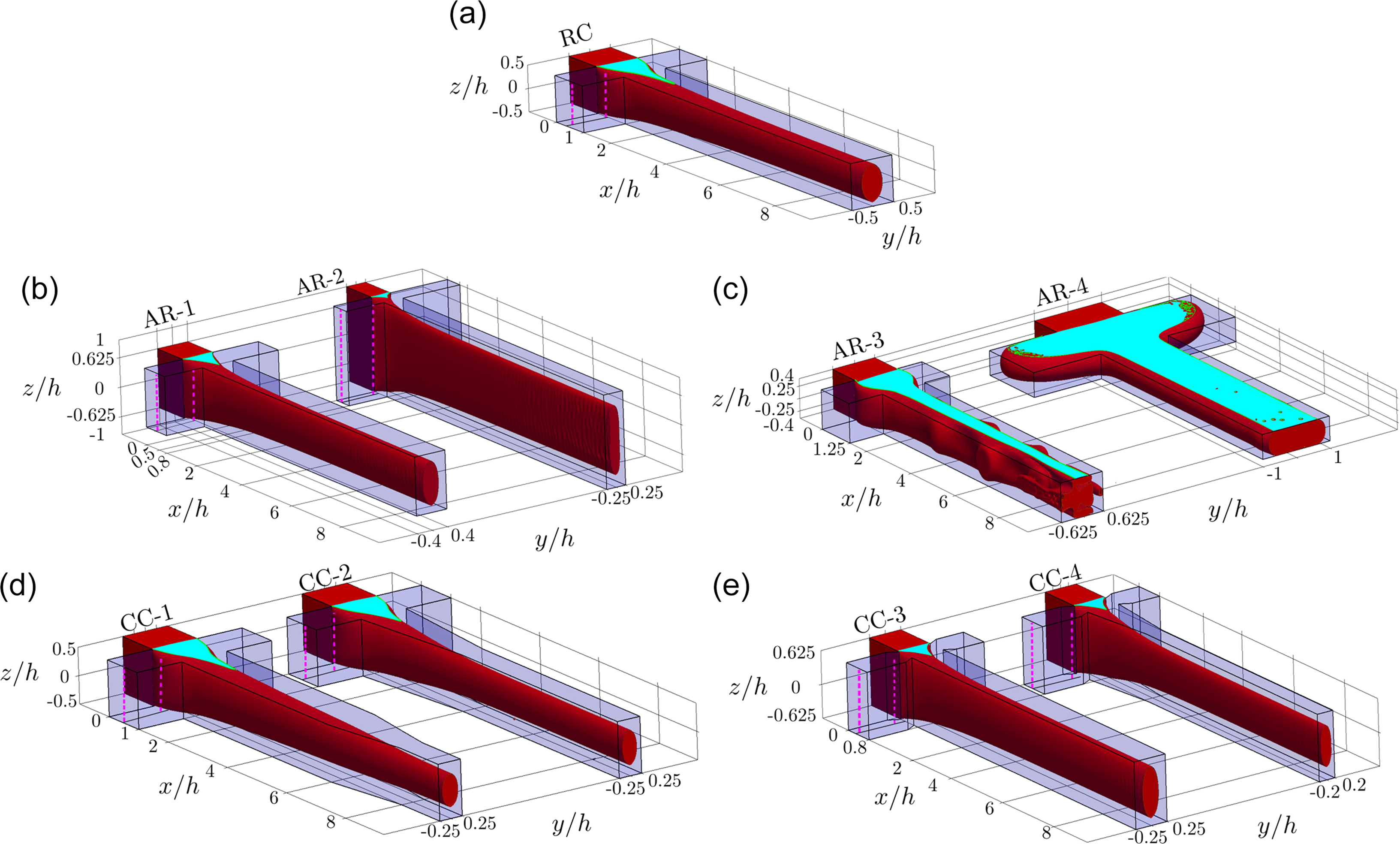
3.2.2. Thread shapes
Figure 8 shows the 3-D shape of the core fluid thread for all the nine configurations. The aqua colour at the top plane of the respective geometry indicates the region wetted by the core fluid dispersion before the detachment from the top and bottom channel walls. Depending on the cross-sectional aspect ratio $\alpha$
of the channel arms (see table 1), thread shapes vary.
$\alpha$
of the channel arms (see table 1), thread shapes vary.
For the AR-1 and AR-2 cases, where $\alpha$ $\gt$
1, the threads are thinner, and the wetted regions are shorter as compared with the RC (
$\gt$
1, the threads are thinner, and the wetted regions are shorter as compared with the RC ( $\alpha =1$
) case. On the other hand, for the AR-3 and AR-4 cases, where
$\alpha =1$
) case. On the other hand, for the AR-3 and AR-4 cases, where $\alpha =1$
, the core fluid remains attached to the top and bottom channel walls (indicated by aqua colour) all along the outlet channel length, and eventually develops instabilities far downstream. For CC-1 to CC-4, where
$\alpha =1$
, the core fluid remains attached to the top and bottom channel walls (indicated by aqua colour) all along the outlet channel length, and eventually develops instabilities far downstream. For CC-1 to CC-4, where $\alpha \geq 1$
, figure 8(d,e) shows that the effect of converging sections appears to impact both the thread shape and wetted regions.
$\alpha \geq 1$
, figure 8(d,e) shows that the effect of converging sections appears to impact both the thread shape and wetted regions.
In order to comprehend the variations in the thread features among all the configurations, a quantitative analysis is carried out utilising the sheath flow velocity profiles, wetted lengths $L_{w}/h$
and the thread aspect ratio
$L_{w}/h$
and the thread aspect ratio $\varepsilon _{z}/\varepsilon _{y}$
as detailed below. Besides, as the flow is unstable in the AR-3 and AR-4 configurations, these two cases are excluded from the following analysis.
$\varepsilon _{z}/\varepsilon _{y}$
as detailed below. Besides, as the flow is unstable in the AR-3 and AR-4 configurations, these two cases are excluded from the following analysis.
3.2.3. Velocity profiles and wetted length
Figure 9 shows the sheath flow velocity profiles as a function of normalised channel height ( $z/z_{\textrm {max}}$
) at different
$z/z_{\textrm {max}}$
) at different $y/h$
locations (upstream and downstream as indicated by dashed magenta lines in figure 8) together with the wetted region shapes for all the geometrical configurations. Note that
$y/h$
locations (upstream and downstream as indicated by dashed magenta lines in figure 8) together with the wetted region shapes for all the geometrical configurations. Note that $U$
represents the velocity magnitude in the
$U$
represents the velocity magnitude in the $x$
direction. In all the cases, the upstream location is near the sheath flow inlet after the flow is fully developed, and the downstream position is near the focusing region.
$x$
direction. In all the cases, the upstream location is near the sheath flow inlet after the flow is fully developed, and the downstream position is near the focusing region.
(a–c) Cases RC, AR-1 and AR-2; (d–f) RC, CC-1 to CC-4. Sheath flow velocity profiles as a function of normalised channel height ( $z/z_{\textrm {max}}$
) at upstream (a,d) and downstream (b,e)
$z/z_{\textrm {max}}$
) at upstream (a,d) and downstream (b,e) $y/h$
locations (indicated by dashed magenta lines in figure 8). In (c,f), the top rows show the wetted region morphologies. The filled symbols in both top and bottom rows depict the wetted lengths
$y/h$
locations (indicated by dashed magenta lines in figure 8). In (c,f), the top rows show the wetted region morphologies. The filled symbols in both top and bottom rows depict the wetted lengths $(L_{w}/h)$
of respective geometrical configurations.
$(L_{w}/h)$
of respective geometrical configurations.
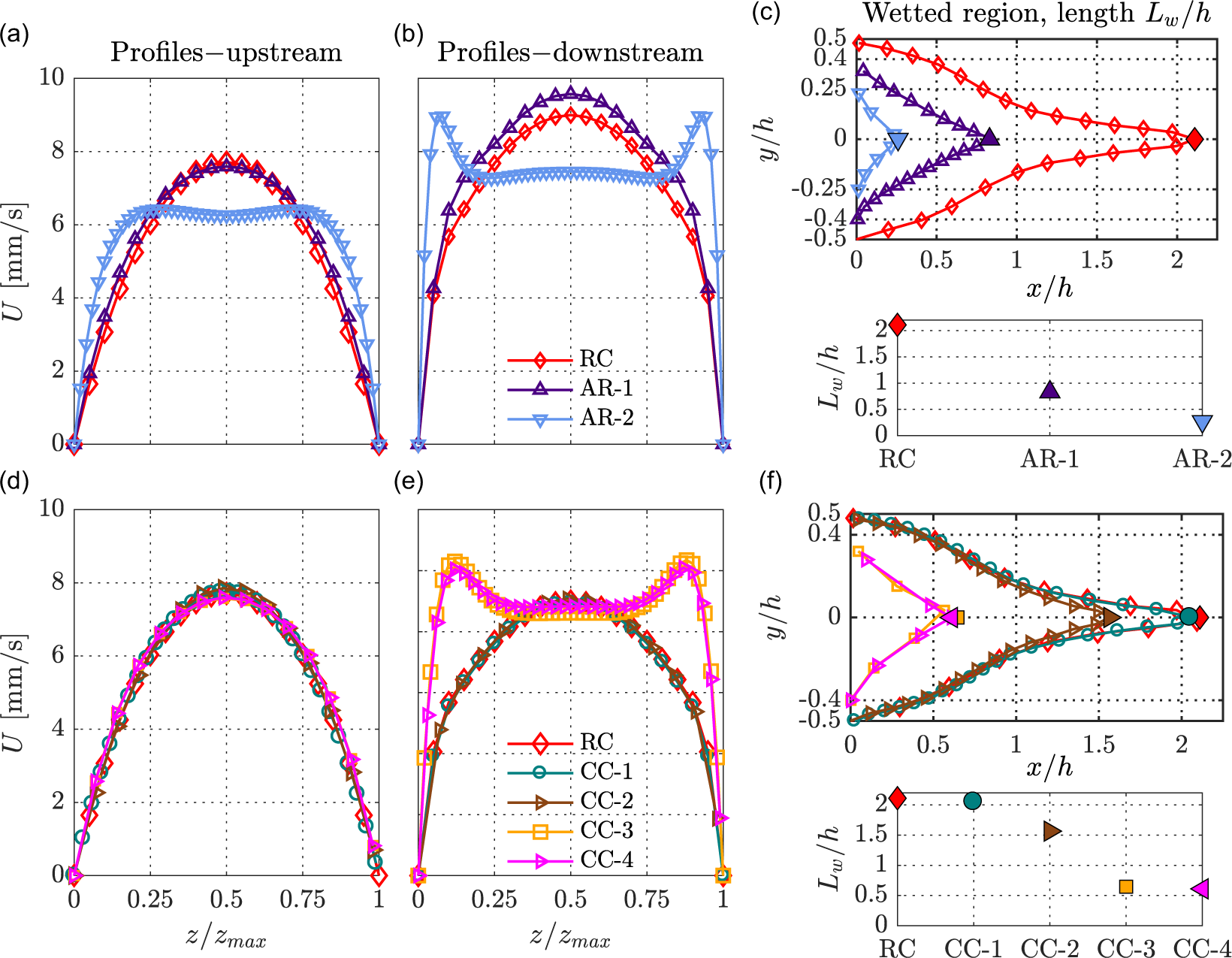
As seen from figure 9(a), the upstream sheath flow velocity profile is parabolic in both RC and AR-1 (aspect ratio $\alpha = 1 \ \text{and} \ 1.56$
) cases, while in the AR-2 case, the profile exhibits a plug-flow-like behaviour due to the higher aspect ratio (
$\alpha = 1 \ \text{and} \ 1.56$
) cases, while in the AR-2 case, the profile exhibits a plug-flow-like behaviour due to the higher aspect ratio ( $\alpha = 4$
) of the sheath flow channel arms. Further downstream, as observed in figure 9(b), the profiles in RC and AR-1 cases display more or less parabolic shapes with a slightly higher magnitude in the AR-1 case. In the case of AR-2, the velocity profile is uniform for most of the channel height except closer to the channel walls where the velocity is high.
$\alpha = 4$
) of the sheath flow channel arms. Further downstream, as observed in figure 9(b), the profiles in RC and AR-1 cases display more or less parabolic shapes with a slightly higher magnitude in the AR-1 case. In the case of AR-2, the velocity profile is uniform for most of the channel height except closer to the channel walls where the velocity is high.
The downstream sheath flow velocity profiles influence the core fluid thread detachment, i.e. the wetted lengths $L_w/h$
, as depicted in figure 9(c). The plug-flow profile in the AR-2 case leads to an early detachment of the core fluid thread from the top and bottom channel walls, leading to a shorter
$L_w/h$
, as depicted in figure 9(c). The plug-flow profile in the AR-2 case leads to an early detachment of the core fluid thread from the top and bottom channel walls, leading to a shorter $L_w/h \simeq 0.27$
, compared with AR-1 (
$L_w/h \simeq 0.27$
, compared with AR-1 ( $L_w/h \simeq 0.83$
) and RC (
$L_w/h \simeq 0.83$
) and RC ( $L_w/h \simeq 2.1$
) cases. All the values of
$L_w/h \simeq 2.1$
) cases. All the values of $L_w/h$
in the different cases are tabulated in table 1.
$L_w/h$
in the different cases are tabulated in table 1.
Continuing to the upstream velocity profiles of the sheath flow in RC and CC-1 to CC-4 cases, as seen from figure 9(d), the velocity profiles are parabolic. At this point, it is worth recalling that the aspect ratio $\alpha$
of the inlet channel arms of CC-1 and CC-2 cases is the same as that of the RC case (
$\alpha$
of the inlet channel arms of CC-1 and CC-2 cases is the same as that of the RC case ( $\alpha = 1$
), while that of CC-3 and CC-4 cases corresponds to that of the AR-1 (
$\alpha = 1$
), while that of CC-3 and CC-4 cases corresponds to that of the AR-1 ( $\alpha = 1.56$
) case.
$\alpha = 1.56$
) case.
At the downstream position (figure 9
e), the velocity profiles of CC-1 and RC cases overlap each other as expected, since both configurations have the same $\alpha$
, and as such, there is no influence of the converging section, which is 5 mm downstream from the confluence region. Also, the wetted length
$\alpha$
, and as such, there is no influence of the converging section, which is 5 mm downstream from the confluence region. Also, the wetted length $L_{w}/h$
(figure 9
f,
$L_{w}/h$
(figure 9
f, $L_{w}/h \simeq 2.1$
) is the same, with and without the converging section. However, in the CC-2 case, the converging section begins right at the end of the confluence region
$L_{w}/h \simeq 2.1$
) is the same, with and without the converging section. However, in the CC-2 case, the converging section begins right at the end of the confluence region $x/h = 1$
. Also here, the velocity profiles (figure 9
e) overlap with the RC case, but the wetted length
$x/h = 1$
. Also here, the velocity profiles (figure 9
e) overlap with the RC case, but the wetted length $L_{w}/h$
(see figure 9
f) in the CC-2 case (
$L_{w}/h$
(see figure 9
f) in the CC-2 case ( $L_{w}/h \simeq 1.5$
) is shorter than that in the RC case (
$L_{w}/h \simeq 1.5$
) is shorter than that in the RC case ( $L_{w}/h \simeq 2.1$
). This difference in
$L_{w}/h \simeq 2.1$
). This difference in $L_{w}/h$
could be attributed to the converging section.
$L_{w}/h$
could be attributed to the converging section.
On the other hand, figure 9(e,f) shows that in cases CC-3 and CC-4, both velocity profiles and the wetted regions almost collapse on top of each other. The uniqueness of these two configurations is with regard to the velocity profiles. Both have the same cross-sectional aspect ratio ( $\alpha = 1.56$
) of the sheath flow inlet channel arms, which is similar to the AR-1 case, but exhibit plug-flow-like flow profiles as observed in the high-aspect-ratio (
$\alpha = 1.56$
) of the sheath flow inlet channel arms, which is similar to the AR-1 case, but exhibit plug-flow-like flow profiles as observed in the high-aspect-ratio ( $\alpha = 4$
) AR-2 configuration (figure 9
b). This, in turn, leads to an early detachment of the core fluid thread with shorter wetted lengths
$\alpha = 4$
) AR-2 configuration (figure 9
b). This, in turn, leads to an early detachment of the core fluid thread with shorter wetted lengths $L_w/h \simeq 0.65$
and
$L_w/h \simeq 0.65$
and $0.61$
(see figure 9
f) compared with
$0.61$
(see figure 9
f) compared with $L_w/h \simeq 0.83$
for the AR-1 case (see figure 9
c). Indeed, this behaviour in both AR-1 and AR-2 configurations could be attributed to the converging sections at the end of the sheath flow inlet channel arms. Meanwhile, the converging section in the core flow inlet channel arm in the CC-4 case could also play a role to some extent, similar to the case of CC-2 resulting in a slightly shorter
$L_w/h \simeq 0.83$
for the AR-1 case (see figure 9
c). Indeed, this behaviour in both AR-1 and AR-2 configurations could be attributed to the converging sections at the end of the sheath flow inlet channel arms. Meanwhile, the converging section in the core flow inlet channel arm in the CC-4 case could also play a role to some extent, similar to the case of CC-2 resulting in a slightly shorter $L_w/h\simeq 0.61$
compared with
$L_w/h\simeq 0.61$
compared with $L_w/h \simeq 0.65$
for the CC-3 case.
$L_w/h \simeq 0.65$
for the CC-3 case.
Thus, having understood the velocity profiles and wetted lengths of all geometrical configurations, we now examine other aspects such as development of thread aspect ratio $\varepsilon _z/\varepsilon _y$
and strain rate
$\varepsilon _z/\varepsilon _y$
and strain rate $\dot {\varepsilon }$
along the centreline.
$\dot {\varepsilon }$
along the centreline.
3.2.4. Thread aspect ratio and strain rate
(a–c) Cases RC, AR-1 and AR-2; (d–f) RC, CC-1 to CC-4. (a,d) Evolution of thread aspect ratio ( $\epsilon _z/\epsilon _y$
) (normalised with the inlet channel arm cross-sectional aspect ratio
$\epsilon _z/\epsilon _y$
) (normalised with the inlet channel arm cross-sectional aspect ratio $\alpha$
; table 1) as a function of downstream
$\alpha$
; table 1) as a function of downstream $x/h$
positions. (b,e) The maximum (
$x/h$
positions. (b,e) The maximum ( $Ar_{\textrm {max}}$
, open
$Ar_{\textrm {max}}$
, open![]() symbols) and final (
symbols) and final ( $Ar_{\textrm {final}}$
, filled
$Ar_{\textrm {final}}$
, filled![]() symbols) thread aspect ratio
symbols) thread aspect ratio $\varepsilon _z/\varepsilon _y$
for all the geometries. (c,f) Evolution of strain rate
$\varepsilon _z/\varepsilon _y$
for all the geometries. (c,f) Evolution of strain rate $\dot {\varepsilon }$
along the centreline as a function of downstream positions
$\dot {\varepsilon }$
along the centreline as a function of downstream positions $x/h$
.
$x/h$
.

Figure 10 shows the normalised thread aspect ratio ( $\varepsilon _{z}/\varepsilon _{y}$
) and strain rate (
$\varepsilon _{z}/\varepsilon _{y}$
) and strain rate ( $\dot {\varepsilon } = \partial u/{\partial x}$
) along the centreline as a function of downstream
$\dot {\varepsilon } = \partial u/{\partial x}$
) along the centreline as a function of downstream $x/h$
positions together with the maximum (
$x/h$
positions together with the maximum ( $Ar_{\textrm {max}}$
) and final (
$Ar_{\textrm {max}}$
) and final ( $Ar_{\textrm {final}}$
) aspect ratio of the threads. In figure 10(a,d), all the thread aspect ratios
$Ar_{\textrm {final}}$
) aspect ratio of the threads. In figure 10(a,d), all the thread aspect ratios $\varepsilon _{z}/\varepsilon _{y}$
are normalised with the corresponding inlet channel arm cross-sectional aspect ratio
$\varepsilon _{z}/\varepsilon _{y}$
are normalised with the corresponding inlet channel arm cross-sectional aspect ratio $\alpha$
(see table 1). Thus, the thread aspect ratios
$\alpha$
(see table 1). Thus, the thread aspect ratios $\varepsilon _{z}/\varepsilon _{y}$
plotted in figure 10(a,d) for cases AR-1, AR-2, CC-3 and CC-4 are much higher than for the RC case. In figure 10(b,e),
$\varepsilon _{z}/\varepsilon _{y}$
plotted in figure 10(a,d) for cases AR-1, AR-2, CC-3 and CC-4 are much higher than for the RC case. In figure 10(b,e), $Ar_{\textrm {max}}$
and
$Ar_{\textrm {max}}$
and $Ar_{\textrm {final}}$
represent the actual values.
$Ar_{\textrm {final}}$
represent the actual values.
A closer view of figure 10(a) shows that the thread aspect ratio $\varepsilon _{z}/\varepsilon _{y}$
increases in RC, AR-1 and AR-2 cases until the position of thread detachment (see figure 9
c or table 1). Thereafter, the thread shape remains more or less constant. In fact, depending on the channel arm cross-sectional aspect ratio
$\varepsilon _{z}/\varepsilon _{y}$
increases in RC, AR-1 and AR-2 cases until the position of thread detachment (see figure 9
c or table 1). Thereafter, the thread shape remains more or less constant. In fact, depending on the channel arm cross-sectional aspect ratio $\alpha$
(table 1), the cross-sectional shapes of the thread vary. As observed from figure 10(b),
$\alpha$
(table 1), the cross-sectional shapes of the thread vary. As observed from figure 10(b), $Ar_{\textrm {max}}$
and
$Ar_{\textrm {max}}$
and $Ar_{\textrm {final}}$
are highest for the slender channel (AR-2), followed by the AR-1 and RC cases. In all the configurations,
$Ar_{\textrm {final}}$
are highest for the slender channel (AR-2), followed by the AR-1 and RC cases. In all the configurations, $Ar_{\textrm {final}}$
is the mean value of
$Ar_{\textrm {final}}$
is the mean value of $\varepsilon _{z}/\varepsilon _{y}$
for
$\varepsilon _{z}/\varepsilon _{y}$
for $15 \leq x/h \leq 20$
.
$15 \leq x/h \leq 20$
.
The variation in strain rate $\dot {\varepsilon }$
along the centreline in figure 10(c) follows a pattern similar to
$\dot {\varepsilon }$
along the centreline in figure 10(c) follows a pattern similar to $Ar_{\textrm {max}}$
and
$Ar_{\textrm {max}}$
and $Ar_{\textrm {final}}$
. The strain rate
$Ar_{\textrm {final}}$
. The strain rate $\dot {\varepsilon }$
is higher for the slender thread (AR-2 case) compared with AR-1 and RC cases. However, it is important to note that the length of the region where
$\dot {\varepsilon }$
is higher for the slender thread (AR-2 case) compared with AR-1 and RC cases. However, it is important to note that the length of the region where $\dot {\varepsilon }\gt 0$
is the shortest (
$\dot {\varepsilon }\gt 0$
is the shortest ( $0 \leq x/h \leq 2$
) for the AR-2 case, while it is more or less similar (
$0 \leq x/h \leq 2$
) for the AR-2 case, while it is more or less similar ( $0 \leq x/h \leq 4$
) for AR-1 and RC cases.
$0 \leq x/h \leq 4$
) for AR-1 and RC cases.
Turning to the configurations with converging sections, CC-1 to CC-4 cases, figure 10(d) shows that in the case of CC-1, the thread aspect ratio $\varepsilon _{z}/\varepsilon _{y}$
dips for
$\varepsilon _{z}/\varepsilon _{y}$
dips for $6 \leq x/h \leq 8$
. In the CC-2 configuration, the combined effects of sheath flow momentum (
$6 \leq x/h \leq 8$
. In the CC-2 configuration, the combined effects of sheath flow momentum ( $0 \leq x/h \leq 1$
) and the converging section (
$0 \leq x/h \leq 1$
) and the converging section ( $1 \leq x/h \leq 3$
) result in a more pronounced development of the thread with higher
$1 \leq x/h \leq 3$
) result in a more pronounced development of the thread with higher $\varepsilon _{z}/\varepsilon _{y}$
. As seen from figure 10(e), although
$\varepsilon _{z}/\varepsilon _{y}$
. As seen from figure 10(e), although $\alpha = 1$
remains the same in RC, CC-1 and CC-2 cases, the converging sections in CC-1 and CC-2 cases produce higher
$\alpha = 1$
remains the same in RC, CC-1 and CC-2 cases, the converging sections in CC-1 and CC-2 cases produce higher $Ar_{\textrm {max}}$
and
$Ar_{\textrm {max}}$
and $Ar_{\textrm {final}}$
than in the RC case. In fact, the strain rate
$Ar_{\textrm {final}}$
than in the RC case. In fact, the strain rate $\dot {\varepsilon }$
along the centreline in figure 10(f) shows a clear impact of the converging sections, wherein, for the CC-1 case,
$\dot {\varepsilon }$
along the centreline in figure 10(f) shows a clear impact of the converging sections, wherein, for the CC-1 case, $\dot {\varepsilon }$
shoots up for
$\dot {\varepsilon }$
shoots up for $6 \leq x/h \leq 8$
, and in the CC-2 case,
$6 \leq x/h \leq 8$
, and in the CC-2 case, $\dot {\varepsilon } \gt 0$
extends from
$\dot {\varepsilon } \gt 0$
extends from $x/h = 0$
all the way up to
$x/h = 0$
all the way up to $x/h = 5$
.
$x/h = 5$
.
Additionally, in the CC-3 and CC-4 cases, $Ar_{\textrm {max}}$
and
$Ar_{\textrm {max}}$
and $Ar_{\textrm {final}}$
(figure 10
e) are much higher than in RC, CC-1 and CC-3. It is worth recalling that CC-3 and CC-4 are the modified channel configurations with
$Ar_{\textrm {final}}$
(figure 10
e) are much higher than in RC, CC-1 and CC-3. It is worth recalling that CC-3 and CC-4 are the modified channel configurations with $\alpha = 1.56$
, which is the same as AR-1. In comparison with AR-1 (figure 10
b,c), the effect of the converging section in the sheath flow inlet in CC-3 appears to be small with a minor increment in
$\alpha = 1.56$
, which is the same as AR-1. In comparison with AR-1 (figure 10
b,c), the effect of the converging section in the sheath flow inlet in CC-3 appears to be small with a minor increment in $Ar_{\textrm {max}}$
,
$Ar_{\textrm {max}}$
, $Ar_{\textrm {final}}$
and strain rate
$Ar_{\textrm {final}}$
and strain rate $\dot {\varepsilon }$
. However, the effect on wetted length
$\dot {\varepsilon }$
. However, the effect on wetted length $L_w/h$
was substantial (see figure 9
f).
$L_w/h$
was substantial (see figure 9
f).
Addition of a converging section downstream of the confluence region in the streamwise $x$
direction, as in the case of CC-4, brings in a substantial increase in
$x$
direction, as in the case of CC-4, brings in a substantial increase in $Ar_{\textrm {max}}$
and
$Ar_{\textrm {max}}$
and $Ar_{\textrm {final}}$
of the thread aspect ratio and the strain rate
$Ar_{\textrm {final}}$
of the thread aspect ratio and the strain rate $\dot {\varepsilon }$
as depicted in figure 10(e,f).
$\dot {\varepsilon }$
as depicted in figure 10(e,f).
Summing up, from the thread detachment or wetted length $L_w/h$
point of view, the AR-2 configuration with the channel cross-sectional aspect ratio of
$L_w/h$
point of view, the AR-2 configuration with the channel cross-sectional aspect ratio of $\alpha = 4$
is the ideal choice, since
$\alpha = 4$
is the ideal choice, since $L_w/h \simeq 0.25$
is the shortest. However, from the alignment of nanofibrils perspective, the narrow or smaller length of the strain rate
$L_w/h \simeq 0.25$
is the shortest. However, from the alignment of nanofibrils perspective, the narrow or smaller length of the strain rate $\dot {\varepsilon }$
region in AR-2 geometry could plausibly make it less effective. Therefore, from a break-even point of view, i.e. for achieving the shortest wetted length
$\dot {\varepsilon }$
region in AR-2 geometry could plausibly make it less effective. Therefore, from a break-even point of view, i.e. for achieving the shortest wetted length $L_w/h$
and a wider or longer extent of the strain rate
$L_w/h$
and a wider or longer extent of the strain rate $\dot {\varepsilon }$
region, CC-4 would be a near-optimal choice. Adjusting the length of the converging section (
$\dot {\varepsilon }$
region, CC-4 would be a near-optimal choice. Adjusting the length of the converging section ( $l_{c}$
) in the streamwise
$l_{c}$
) in the streamwise $x$
direction, the strain rate
$x$
direction, the strain rate $\dot {\varepsilon }$
region could be expanded to longer lengths in the CC-4 configuration as well.
$\dot {\varepsilon }$
region could be expanded to longer lengths in the CC-4 configuration as well.
3.2.5. Simulated nanofibril alignment in the additional geometries
(a–c) Streamwise development of mean order parameter $S$
(a),
$S$
(a), $\Delta S$
(b) and
$\Delta S$
(b) and $S/ \Delta S$
(c) as a function of downstream
$S/ \Delta S$
(c) as a function of downstream $x/h$
positions for RC, AR-1 and AR-2 geometries. The black square
$x/h$
positions for RC, AR-1 and AR-2 geometries. The black square![]() symbols on the horizontal axis in (a) correspond to the streamwise
symbols on the horizontal axis in (a) correspond to the streamwise $x/h$
positions of the cross-sectional contours depicted in (e,f). (d–f) Cross-sectional contours of local order parameter
$x/h$
positions of the cross-sectional contours depicted in (e,f). (d–f) Cross-sectional contours of local order parameter $S_{\textrm {local}}$
, at different streamwise
$S_{\textrm {local}}$
, at different streamwise $x/h$
positions. As indicated in (d), in (e,f), the top-half segment represents the RC case and the bottom half represents AR-1 and AR-2 cases.
$x/h$
positions. As indicated in (d), in (e,f), the top-half segment represents the RC case and the bottom half represents AR-1 and AR-2 cases.
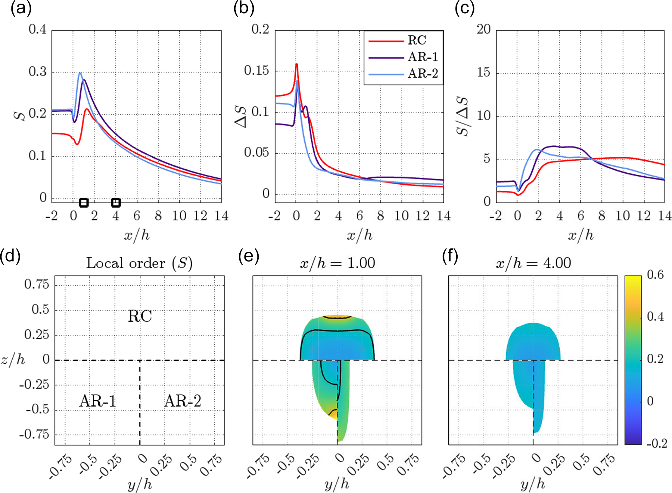
Finally, the fibril alignment in the six geometries of figure 8 is studied numerically. The results are presented in figures 11 and 12 for the AR and CC geometries, respectively. In both figures, panel (a) shows streamwise development of the mean order parameter $S$
, panel (b) the variance of the local order parameter over the cross-section
$S$
, panel (b) the variance of the local order parameter over the cross-section $\Delta S$
and panel (c)
$\Delta S$
and panel (c) $S/\Delta S$
, i.e. the ratio between alignment and its variation over the cross-section. Again, a high value of
$S/\Delta S$
, i.e. the ratio between alignment and its variation over the cross-section. Again, a high value of $S/\Delta S$
typically indicates a high degree of alignment with limited variation over the cross-section. In panels (e) and (f), the distribution of the local order parameter over the cross-section is shown with one geometry per quadrant as indicated in panel (d). A first observation is expected, namely that the alignment development in figures 12(a) and 11(a) is explained by the strain rate
$S/\Delta S$
typically indicates a high degree of alignment with limited variation over the cross-section. In panels (e) and (f), the distribution of the local order parameter over the cross-section is shown with one geometry per quadrant as indicated in panel (d). A first observation is expected, namely that the alignment development in figures 12(a) and 11(a) is explained by the strain rate $\dot {\varepsilon }$
development shown in figure 10(c,f).
$\dot {\varepsilon }$
development shown in figure 10(c,f).
(a–c) Streamwise development of mean order parameter $S$
(a),
$S$
(a), $\Delta S$
(b) and
$\Delta S$
(b) and $S/ \Delta S$
(c) as a function of downstream
$S/ \Delta S$
(c) as a function of downstream $x/h$
positions for RC and CC-1 to CC-4 geometries. The black square
$x/h$
positions for RC and CC-1 to CC-4 geometries. The black square![]() symbols on the horizontal axis in (a) correspond to the streamwise
symbols on the horizontal axis in (a) correspond to the streamwise $x/h$
positions of the cross sectional contours depicted in (e,f). (d–f) Cross-sectional contours of local order parameter
$x/h$
positions of the cross sectional contours depicted in (e,f). (d–f) Cross-sectional contours of local order parameter $S_{\textrm {local}}$
, at different streamwise
$S_{\textrm {local}}$
, at different streamwise $x/h$
positions. In (e,f), each quarter segment represents different geometrical cases of CC-1 to CC-4 as indicated in (d).
$x/h$
positions. In (e,f), each quarter segment represents different geometrical cases of CC-1 to CC-4 as indicated in (d).
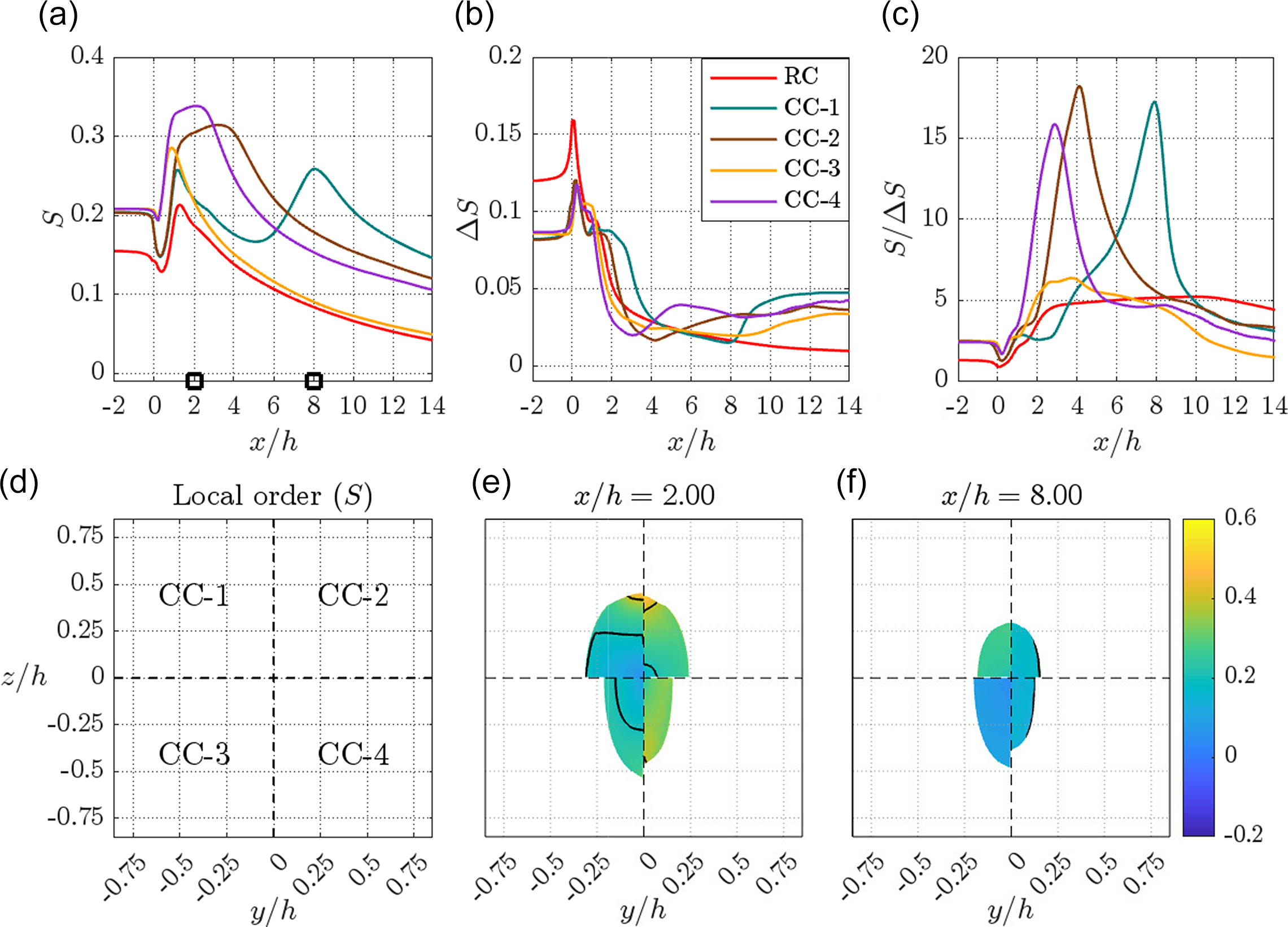
The AR geometries (figure 11) are seen to give a slightly higher maximum alignment and similar variation $\Delta S$
as compared to RC (
$\Delta S$
as compared to RC ( $\beta =90^\circ$
). The differences, both with respect to the RC and between the geometries, are more pronounced for the CC geometries shown in figure 12. Compared with RC, the CC geometries produce higher maximum alignment with very small variation over the cross-section, in particular for CC-1, CC-2 and CC-4. The streamwise position of the maximum of
$\beta =90^\circ$
). The differences, both with respect to the RC and between the geometries, are more pronounced for the CC geometries shown in figure 12. Compared with RC, the CC geometries produce higher maximum alignment with very small variation over the cross-section, in particular for CC-1, CC-2 and CC-4. The streamwise position of the maximum of $S/\Delta S$
varies and it is clear that the geometry can be designed to deliver high alignment at a certain position. This is of great interest in assembly application, where chemical reactions locking the aligned structure (e.g. pH-controlled gelation or light-induced polymerisation) could be tuned to act at the position of highest alignment.
$S/\Delta S$
varies and it is clear that the geometry can be designed to deliver high alignment at a certain position. This is of great interest in assembly application, where chemical reactions locking the aligned structure (e.g. pH-controlled gelation or light-induced polymerisation) could be tuned to act at the position of highest alignment.
Peak value of the mean order $S_{\textrm {max}}$
(horizontal axis) and the order homogeneity measure
$S_{\textrm {max}}$
(horizontal axis) and the order homogeneity measure $S_{\textrm {max}}/\Delta S$
(vertical axis) for all geometries as defined in the legend.
$S_{\textrm {max}}/\Delta S$
(vertical axis) for all geometries as defined in the legend.
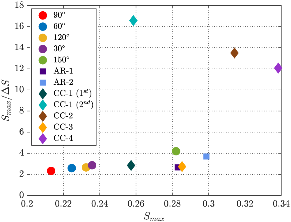
The alignment results in terms of $S_{\textrm {max}}$
and
$S_{\textrm {max}}$
and $S_{\textrm {max}}/\Delta S$
for all geometries are summarised in figure 13. The preferred situation, high alignment with small variation, corresponds to the upper-right corner. The importance of contractions is again very clear, since the previously identified CC-1, CC-2 and CC-4 stand out from the other geometries. It is also worth noting that all geometries perform better than RC (
$S_{\textrm {max}}/\Delta S$
for all geometries are summarised in figure 13. The preferred situation, high alignment with small variation, corresponds to the upper-right corner. The importance of contractions is again very clear, since the previously identified CC-1, CC-2 and CC-4 stand out from the other geometries. It is also worth noting that all geometries perform better than RC ( $\beta =90^\circ$
).
$\beta =90^\circ$
).
4. Conclusions
Building on previous combined experimental and numerical method development, the flow and fibril alignment in 11 different flow geometries have been studied. It was demonstrated how the flow geometry can be used to control thread detachment or wetted length $L_{w}/h$
, thread aspect ratio
$L_{w}/h$
, thread aspect ratio $\varepsilon _{z}/\varepsilon _{y}$
and fibril alignment. The work is motivated by a desire to understand and control the assembly of nanostructured material in micrometre- and millimetre-sized flow systems.
$\varepsilon _{z}/\varepsilon _{y}$
and fibril alignment. The work is motivated by a desire to understand and control the assembly of nanostructured material in micrometre- and millimetre-sized flow systems.
First, the orientation (or alignment) modelling was seen to be able to capture some, but not all, of the differences in SAXS measurements in flow-focusing geometries with confluence angle $\beta =$
90
$\beta =$
90 $^\circ$
, 60
$^\circ$
, 60 $^\circ$
and 120
$^\circ$
and 120 $^\circ$
. Based on the numerical results, it could be concluded that the alignment behaviour varies much more between the other geometries. As expected, the geometries with a contraction in the outlet channel (CC-1, CC-2 and CC-4; see figure 8) generate high alignment with a small variation over the cross-section.
$^\circ$
. Based on the numerical results, it could be concluded that the alignment behaviour varies much more between the other geometries. As expected, the geometries with a contraction in the outlet channel (CC-1, CC-2 and CC-4; see figure 8) generate high alignment with a small variation over the cross-section.
In flow-focusing spinning, thread formation in the channel is critical. In this context, it was demonstrated that a short contraction in the side-flow channels immediately before the confluence region is an efficient means to promote thread detachment from the top and bottom channel walls. This is achieved as a result of the plug-like velocity profiles that are generated by the contractions, with high-momentum side flows close to the top and bottom walls. This high momentum increases the ability of the side flows with low-viscosity fluid to engulf the core flow of high-viscosity fluid.
In a wider perspective, the present work paves the way for optimising the flow geometries for tailored assembly of macroscopic materials from anisotropic nanoscale building blocks.
Data availability
Data are available upon request from the corresponding author.
Author contributions
K.O.: conceptualisation, orientation simulations, writing; V.K.G.: conceptualisation, flow simulations, X-ray experiments, writing; T.R.: X-ray experiments, editing; S.V.R.: X-ray experiments, editing; L.D.S.: supervision, editing; J.S.: editing, supervision; F.L.: conceptualisation, orientation simulations, X-ray experiments, writing, supervision.
Funding
Financial support from FORMAS (the Swedish Research Council for Sustainable Development), the Swedish Energy Agency, the Swedish Research Council, Knut and Alice Wallenberg Foundation via Wallenberg Wood Science Center and the JST Adopting Sustainable Partnerships for Innovative Research Ecosystem (ASPIRE) programme (grant number JPMJAP2310) is gratefully acknowledged. Computational resources were provided by National Academic Infrastructure for Supercomputing in Sweden (NAISS).
Competing interests
The authors declare no conflict of interest.
Ethical standards
The research meets all ethical guidelines, including adherence to the legal requirements of the study country.


 Open access