

Analysis of archaeological context depends on the three-dimensional location of finds. Provenience, interpreted within a horizontal and vertical stratigraphic framework, relates all other types of data. The quality of spatial data is determined by a combination of precision, accuracy, and quantity. Various technologies from tape measures and optical levels to electronic distance measurers like total stations enable the recording of position, orientation, and scale.
Global navigation satellite systems (GNSS) are the most promising geolocation technology to have emerged in recent decades. The U.S. national system—the global positioning system (GPS)—has been widely recognized and adopted, but other nations provide similar GNSS services. When deployed in the specific configuration of differential GNSS (dGNSS), this technology can provide immediate real-world coordinates with centimeter-level precision. The relevance to archaeological fieldwork is clear; however, prohibitively expensive equipment has limited the use of dGNSS to projects with abundant resources; moreover, these projects deploy only a single measuring system. Recent advances in technological design and manufacturing make possible the provision of a full dGNSS setup for the price of a decent laptop, ultimately enabling the simultaneous use of many devices.
Several companies recently began offering products that provide centimeter-precise locational measurement at an affordable price; we tested one of these products, the Emlid-produced Reach, during an archaeological survey in Armenia in June 2018. Our highly mobile regional survey presented a unique opportunity to test the field suitability, portability, and general ease of use of the dGNSS hardware. We developed an open-source Android app to increase the efficiency of the recording process and to integrate the Reach into our documentation system. Our survey experimented with a point-based recording method, capturing the exact location and an in situ photograph of every find. Traditionally, surveys have had less stringent requirements for precise spatial recording than stratigraphic excavation, which offered us the flexibility to experiment. Yet, emerging technologies mean that archaeological projects can employ high-quality recording with minimal trade-offs in cost or efficiency.
This article advances the archaeological community's ongoing conversation about high-quality spatial field recording (Galeazzi Reference Galeazzi2016; Limp Reference Limp, Forte and Campana2016; Opitz and Herrmann Reference Opitz and Herrmann2018; Smith and Levy Reference Smith and Levy2012). Although surface depositional processes affect the current location of surface finds, location remains our only provenience information for these finds. Places around the world are undergoing constant transformation processes, both anthropogenic and natural; therefore, we archaeologists should record surface finds as precisely and with as much information as possible to preserve this cultural heritage information.
DIGITAL SPATIAL RECORDING TECHNOLOGY IN ARCHAEOLOGY
Archaeologists have always sought to geo-reference data, but the advent of digital technologies has led to a step increase in the accuracy and precision of measurements. In this section, we situate our experiment within the history and future of geolocation technologies for archaeological field recording. We compare the relative strengths and weaknesses of various technologies for collecting immediate real-world 3-D coordinate data. Inexpensive dGNSS is a new solution to meet this need.
One common geolocation technology used in archaeology is the total station, having been deployed at field projects since at least the 1980s (Davey Reference Davey1986:56; Elson and Doelle Reference Elson and Doelle1987) and gaining increasing popularity during the 1990s (Rick Reference Rick1996). A total station measures distance with a laser pulse reflection, a simple form of light detection and ranging (lidar). Lidar records the time it takes for emitted light to reflect off a target and return to the device, calculating distance based on the speed of light constant (Schwarz Reference Schwarz2010; Toth and Jóźków Reference Toth and Jóźków2016). The direction of emission is measured mechanically, with pitch based on the deviation from the direction of gravity and the horizontal angle (azimuth) based on the rotation of the device. Combining vertical and horizontal angles with distance, the device automatically triangulates the 3-D coordinate of the target point relative to the device's location. The system's inefficiencies arise from the limitation of single point measurements with manual operation and the targeting of an optical reflector (prism) held by a second person. Total stations are relatively expensive, limiting their deployment, but projects value their ability to obtain subcentimeter precision at close range (Peng et al. Reference Peng, Lin, Guo, Wang and Gao2017).
More advanced lidar systems have great potential for measuring space and have already enabled archaeological discoveries (Chase and Chase Reference Chase, Chase, Masini and Soldovieri2017; Friedman et al. Reference Friedman, Sofaer and Weiner2017; Inomata et al. Reference Inomata, Triadan, Pinzón, Burham, Ranchos, Aoyama and Haraguchi2018; Stenborg et al. Reference Stenborg, Schaan and Figueiredo2018). Ground-based (often simply called 3-D laser scanning) and aerial lidar have also been deployed at archaeological field projects for more than two decades (e.g., Kleiner and Wehr Reference Kleiner and Wehr1994; Opitz and Cowley Reference Opitz, Cowley, Opitz and Cowley2013; Remondino et al. Reference Remondino, Girardi, Rizzi and Gonzo2009), but prohibitive costs make their application exceptionally rare. Lidar scales up distance measurement recording significantly by automatically changing the direction of the light pulse to cover a large area quickly. Capturing data in a cylindrical area around the device through pulse rotation enables millions of points to be recorded in seconds as a continuous point cloud. Measurement of the pulse reflection's properties can also provide information about the material or color of the target object, and parts of the pulse can penetrate vegetation.
Neither a total station nor lidar provides real-world coordinates because each measures relative distance rather than computes absolute geographical location. These devices, however, do provide absolute scale and relative orientation, information transformable into real-world coordinates by establishing the position and orientation of the device before data collection or by geolocating previously captured points. Total stations and lidar require a direct line of sight between the device and the target (Chase and Chase Reference Chase, Chase, Masini and Soldovieri2017). Lidar holds great potential for recording spatial archaeological data and will likely become ubiquitous on field projects once it is affordable. Industrial applications in robotics, including autonomous automobiles, are driving decreases in cost. At the start of 2018, a major lidar producer made headlines by cutting the price of popular devices in half (see https://www.cnet.com/roadshow/news/velodyne-just-made-self-driving-cars-a-bit-less-expensive-hopefully/). Most archaeological projects will likely eventually deploy unmanned aerial vehicle (UAV)-based lidar systems for periodic scanning of entire archaeological sites and landscapes. Many archaeologists are also using highly affordable photogrammetry to produce 3-D spatial models from simple photographs (Sapirstein and Murray Reference Sapirstein and Murray2017). This method, however, does not directly record absolute scale and currently cannot return immediate measurements or real-world coordinates.
In contrast to lidar, GNSS devices trilaterate position by measuring the arrival time of radio signals from at least four satellites at known orbital locations. Environmental factors like the atmosphere cause signal errors, resulting in absolute measurement accuracies of a few meters. However, differential GNSS (dGNSS) corrects for errors by placing two devices sufficiently near to one another (usually within about 10 km) to detect the same group of satellites and experience the same sources of atmospheric and other noise. One device, the base station, remains stationary on a known point throughout the measurement activities. This base continuously calculates the current error between its known position and the satellite-provided position, the differential of dGNSS. A second GNSS device, called the rover, collects mobile points. The rover communicates with the base via a local radio connection or over the Internet to receive the error corrections, resulting in real-time measurements accurate within centimeters, relative to the base's position.
Because of the high level of mobility of the rover, this type of dGNSS is often also referred to as real-time kinetic (RTK). RTK is distinguished from an older form of dGNSS consisting of a base and rover that were not in immediate contact, requiring the corrections to be applied later in postprocessing. Because the differential error correction is the most fundamental part of the process, and hardware and network advances now make almost all corrections in real time, we refer to the overall method and equipment as dGNSS, rather than RTK.
Differential GNSS has several features that differentiate it from other spatial recording techniques. Although lacking a line-of-sight requirement, both the base and rover need to receive signals from at least four of the same satellites. Landscape elements may obstruct the signals, so some operational environments, including dense forest, urban spaces, caves, or deep valleys, preclude the use of GNSS. Unlike lidar, dGNSS records single points, but in contrast to a total station, a single person can quickly record each point by placing the rover directly over the point. Like a total station's reflector, a leveled surveying rod often holds a rover to record data at a convenient height above any close obstructions. Once a dGNSS base station is established, a single user can capture high-precision real-world coordinates in just a few seconds with the rover, which is a distinct advantage.
Several companies have begun producing dGNSS devices that are significantly less expensive than lidar. These new dGNSS devices are generally targeted at the technology developer market for direct integration into build-your-own UAVs (drones) and require specialized knowledge for deployment. Rendered affordable because of GNSS frequency band limitations, these new dGNSSs use only the L1 frequency band of GPS or the equivalent for other GNSS networks: for example, QZSS L1 (Japan), GLONASS G1 (Russia), BeiDou B1 (China), and Galileo E1 (the European Union). L1 was the first civilian band authorized in 1993 (Eissfeller et al. Reference Eissfeller, Ameres, Kropp and Sanroma2007). Since then, several new frequency bands (L2C, L5, and L1C) offer higher power transmission, more bandwidth, and other upgraded features, such as faster signal acquisition, better performance under vegetative cover, greater reliability (more stable “fixed” status), and increased accuracy, particularly in the vertical direction (GPS.gov 2017). However, equipment that leverages these extra bands remains prohibitively expensive.
Several affordable dGNSS products have arrived on the market in recent years. Swiftnav sells the Piksi Multi Evaluation Kit, with two circuit-board–based GNSS devices, antennas, and other components ($2,000; https://www.swiftnav.com/piksi-multi). ProfiCNC markets the Here+, designed to directly integrate with a UAV flight controller ($600; http://www.proficnc.com/content/12-here). EFarmer will soon release the FieldBee and Bee Station to guide agricultural equipment ($2,000; https://efarmer.mobi/). A company called Emlid, based in St. Petersburg, Russia, began selling the Reach a few years ago, which has since been upgraded to the Reach M+ and Reach RS+ ($1,200 together; https://store.emlid.com/product/reach-mapping-kit).
We purchased a Reach and a Reach RS in early 2017 and field tested them in summer 2018. The Reach came as a circuit board with a separate antenna and was attractive because of its $250 price. The Reach RS integrates a battery and an antenna in a rugged case and is readily deployable for outdoor use. The combination of low price and easy deployment potential attracted us to these two products. Our comparative testing of multiple vendors’ products was prevented by resource constraints common to archaeology.
SURVEY MEASUREMENT QUALITY
Over many decades, archaeological survey methods have become increasingly systematic and precise (Alcock and Cherry Reference Alcock and Cherry2016; Banning Reference Banning2002; Cherry Reference Cherry, Keller and Rupp1983), and technological improvements should enable this trajectory to be continued. Survey fieldwork is assessed according to two measurement qualities: the resolution of sampled data collection and the precision and accuracy of the locational information (points and polygons) that describe the sampling units. Our project aims to enhance the resolution of data collection through efficient digital workflows, while at the same time increasing the precision of locational measurements using dGNSS.
Every field project should specify the resolution of data collection in its sampling strategy. A project may choose to sample areas of arbitrary size such as gridded zones or agricultural fields. Because all finds are counted together within the specified survey unit, the actual provenience of an individual find within that survey area is not recorded. Thus, the resolution of the identifiable context of an individual find is only at the level of the entire survey unit, whether it is gridded squares 5–25 m on a side at a single site or areas of a landscape that are 100–200 m on a side. The advent of inexpensive GNSS has enabled higher-resolution data collection at some projects, with the recording of point locations for individual finds but only at the relatively low precision of a single GNSS device.
Resolution consistency is another important factor. Although a project may be collecting individual points for most of its finds, the team may feel it is onerous to maintain this level of collection resolution when walking through a high-density area of finds. For such an area, they may record a central point or boundary polygon as the interpretive unit of a site. The resolution of contextual knowledge thus changes between finds, with some having individual locations and others only designated as near a central site point or within a site polygon. Whatever method is employed, a project should also strive to record both absence and presence by recording the exact areas sampled and observed by the field walkers, regardless of finds. Our project's mobile digital recording workflow enables the application of a uniform sampling resolution of one point per find, while simultaneously recording everywhere we made observations.
We characterized the quality of the locational data we collected according to external accuracy, internal accuracy, and precision. External accuracy, or absolute accuracy, indicates that the GNSS device records the correct location on the surface of the earth; however, this is difficult to test given the lack of external standards by which to measure the absolute position of a device. A recent report of the Federal Aviation Administration recorded horizontal GPS accuracy within 2 m (WAAS T&E Team 2017) with high-quality GPS equipment. An average smartphone has an accuracy of about 5 m (van Diggelen and Enge Reference van Diggelen and Enge2015). A Reach GNSS device should have around 2 m absolute accuracy when used alone.
The absolute accuracy of dGNSS depends on the accuracy of the known point of the base station. By recording data at a static position for an extended period of time, it should be possible to capture a higher level of accuracy through data averaging. External accuracy is important for reproducibility of results, such as enabling another archaeologist to revisit individual find spots, and for comparing finds to those recorded by neighboring projects. However, given that everyone currently faces the same constraints on determining absolute accuracy, we consider this type of accuracy to be a relatively low priority.
The qualities of internal accuracy and precision are related. Precision indicates the repeatability of a measurement using the same device. For our dGNSS setup, we wanted to verify that measuring the same place across multiple days leads to repeated measurements with acceptable similarity. Internal accuracy, or relative accuracy, indicates that if the dGNSS records two points as being a certain distance apart, they actually are that distance from each other. The ability of basic GNSS technology to function worldwide enhances our confidence in the internal accuracy of dGNSS. The source of potential error is the distance between the base and the rover. Moving beyond the manufacturer's suggested intradevice distance of 10 km increases errors because the corrections from the base become less relevant for the rover. Given resource constraints in the field, we lacked a way to independently test the internal accuracy of the Reach. We were, however, able to test its precision as explained later.
Technology may soon enable researchers to affordably and efficiently record a precise location for each survey find. Even though surface depositional processes undoubtedly obscure original locations, the fact remains that a find's secondary location is the only spatial information available. All arguments and conclusions extracted from the surface data derive from this positional information and hence the imperative to record carefully (Downey Reference Downey2017). In our field experiment, we were able to photograph each find in situ while simultaneously recording high-precision coordinates and other basic information. Photographs efficiently record significant visual data about the find and its context, providing information about local ground cover, deposition, and object characteristics that may lead to decoration, type, and chronological identifications. Our goal is to increase the quality and quantity of the data we collect in the field without increasing collection time.
FIELDWORK CONTEXT
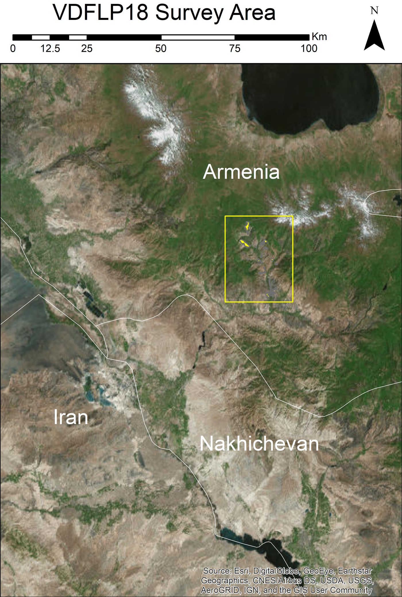
The Vayots Dzor Fortress Landscapes Project (VDFLP) was initiated as a joint Armenian-American project in 2017 by the University of Central Florida and the Institute of Archaeology and Ethnography in Armenia (see https://projects.cah.ucf.edu/armenia/). That year, the project conducted a regional survey in the north–south Yeghegis River valley between the town of Getap and the Selim mountain pass in the Vayots Dzor province, revealing sites and off-site features from the Late Bronze to the medieval periods. The lowest points in the valley are around 900 m asl, whereas the highest points are above 3,000 m asl. The valley zones of Vayots Dzor demonstrate a continental climate typified by hot summers and harsh winters; in contrast, the highland zones have an alpine climate and vegetation. The 2018 survey, sponsored by the Penn Museum of the University of Pennsylvania, built on the results of the 2017 season and provided a context for testing the new dGNSS equipment and workflows (Figure 1).
2018 survey area.
The VDFLP aims to contextualize archaeological finds within the known historical frameworks of the Urartian and medieval Armenian periods by understanding how social processes like warfare affected observed patterns of travel, trade, and habitation (cf. Earley-Spadoni Reference Earley-Spadoni2015; Ristvet Reference Ristvet, Düring and Stek2018). Urartu was a powerful highland empire and a perennial threat to the Neo-Assyrian state. In the eighth century BCE, the Yeghegis Valley was an important corridor connecting Urartian-annexed territories to the south with fortress landscapes near Lake Sevan. During the medieval period, the Vayots Dzor region was ruled by Georgian vassal princes subservient to the Mongol Ilkhanate, and the valley was developed with fortresses, churches, caravanserais, and bridges, effectively incorporating it into the Silk Roads network (Babajanyan and Franklin Reference Babajanyan and Franklin2018). Methodologically, the VDFLP serves as an incubator for digital humanities applications in archaeological research (Earley-Spadoni Reference Earley-Spadoni2017).
METHODS
The Data Collection System
Before we undertook our summer 2018 fieldwork, we implemented and tested a high-precision point-based surface survey data collection workflow. First, we acquired the physical hardware devices and transported them to the field. Second, we configured the dGNSS equipment to record locational information. Third, we developed software, as an Android app, to implement an efficient data collection workflow that would be convenient for field archaeologists (Cobb et al. Reference Cobb, Sigmier, Creamer and French2019).
Hardware
We tested a system made up of two Emlid-produced devices: the Reach and the Reach RS. The Reach is a small circuit board requiring an external antenna and power source, and the Reach RS is packaged in a rugged case with an integrated battery and antenna. We used the less expensive and less mobile Reach circuit board as the base station and the sturdier, more expensive Reach RS as the rover. The Reach retails for $250 and the Reach RS for $800; both are eligible for an educational discount, which was 20% at the time of purchase.
We used a concrete government survey point as our base station (Figure 2), which was centrally located in the survey area near the village of Shatin on a hill overlooking the valley. Each morning, we set up the Reach circuit board on top of the point and retrieved it each afternoon, which reduced the time available in which to conduct the survey. Ideally, we would place the base in a field house, where it could remain for an entire season. Our field house, however, was more than 10 km from the study area, a distance outside the operational requirements of this dGNSS system.
Reach circuit board and antenna, used as the base station and placed on the concrete surveying point.
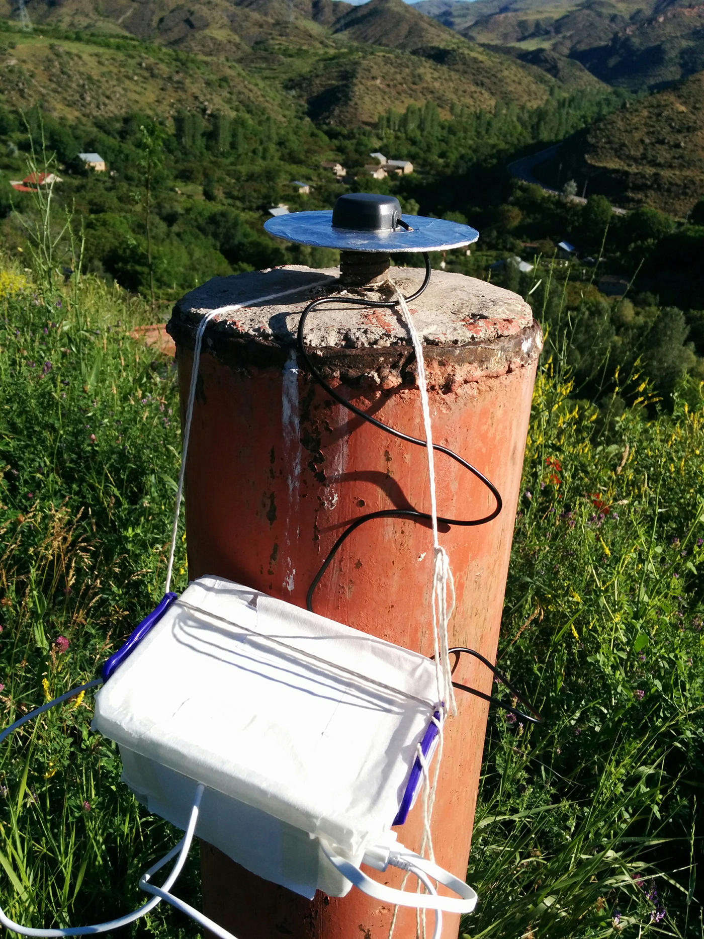
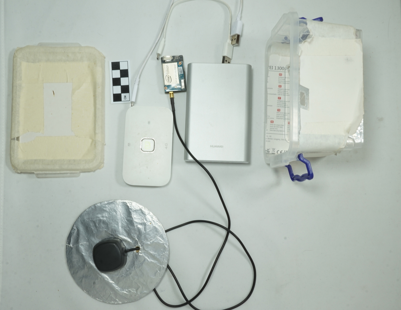
We saved more than $500 by using the Reach circuit board as a base station, reconstructing a package similar to the Reach RS. We acquired a battery bank for $30, with dual USB ports for the Reach and a mobile data modem. The modem provided 4G Internet service through a local cell phone carrier. During the afternoons, the modem served its main function of enabling high-speed Internet in our field house, which was necessary for data entry on our virtual desktop server (Cobb Reference Cobb2017). We borrowed the modem for the month and paid approximately $0.50 per gigabyte of data transfer, although the Reach itself does not use much bandwidth. To protect the components of our base station, we modified a plastic food storage container (Figure 3). The Reach circuit board's antenna also required a custom ground-plane to enhance reception. Points were measured at the antenna receiver, placed in the center of an aluminum-foil–wrapped compact disc–sized piece of cardboard serving as the ground-plane. This antenna receiver was placed directly on the concrete surveying point and was connected to the Reach via its cord.
Base station components: lid, data modem, Reach circuit board, USB battery, plastic food container, and (below) antenna on aluminum foil ground-plane.
To operate the Reach RS rover and collect archaeological data, we deployed Android smartphones that ran our custom app, described later, during field walking. We chose Android because it is the most popular mobile operating system and for its open-source ethos that enables easier development and sharing of code. Additionally, it enabled most of our team members to use their personal devices as data collectors. Smartphone Wi-Fi hot spots gave the rover an Internet connection to receive differential corrections from the base. Another advantage of the Android platform is the wide selection of hardware options available through competing products. We purchased one smartphone, an Asus Zoomphone, for its affordability ($230) and optical zoom feature, which we hoped might save time by not requiring the field walker to bend down to take a photograph. However, we discovered that users needed to place a centimeter scale bar on the ground or hold back vegetation from the find when taking photos.
dGNSS Field Setup
Although GNSS hardware is becoming easier to use, several technical steps are required to ensure proper functionality. Operators must be able to control and configure the hardware, which lacks means of direct input (i.e., through screens or buttons), and the hardware cannot connect to the Internet without the support of a proxy device such as a router or phone hot spot. The user first configures each Reach device by connecting a laptop, smartphone, or tablet directly to the Wi-Fi network run by the Reach. Once connected, a web or mobile application can be used to change the settings of the Reach. A common first step is to configure the Reach to connect to a different Wi-Fi network, enabling it to access the Internet and allowing the user to control the Reach over that external network. Through the Emlid application, one of the Reach devices is designated as the base station and the other as the rover. Users also indicate how the devices will communicate with each other: over radio signals or the Internet. An online tutorial (https://repository.upenn.edu/penn_museum_papers/54/) provides detailed instructions on configuring the Reach devices for dGNSS operation.
Once configured, the rover may be easily moved around to measure points in the field. In our case, the rover used our phone hot spots with a mobile data connection to retrieve base corrections over the Internet. Note that the Reach RS unit is also equipped with a long-range radio (868/915 MHz) unit onboard, allowing for remote communication because of its ability to pass through trees, building materials, and the like (Justice Reference Justice2010). Thus, two Reach RS units can communicate directly over the radio link, rather than relying on a cellular network with limited availability in remote sites. The Emlid blog highlights a recent field test of two Reach RS units reliably communicating using the long-range radio over 1.25 km in a heavily wooded area and over 19 km in a mountainous area (Ershov Reference Ershov2017).
Our phones acquired the points from the rover and presented the current quality of the points, based on a common vocabulary. The rover can operate in one of three different modes— single, float, or fixed—in ascending order of precision (Trimble Navigation Reference Navigation2003). Single indicates that the rover relies entirely on its own receiver and does not take any corrections from the base, resulting in meter-level precision. Float versus fixed mode indicates that different algorithms are used to incorporate corrections from the base. The algorithms calculate the number of radio wavelengths between the satellites and the base. This value can either be a floating point number or an integer (fixed). The float algorithm yields a solution with submeter precision, whereas the fixed mode has centimeter-level precision; therefore, the fixed mode is the preferred method. A variety of reasons, including a low number of visible satellites, poor satellite geometry, or a poor communication link between the base and the rover, may prevent having a fixed solution.
In addition to GPS, the Emlid system also supports SBAS (satellite-based augmentation system) signals. SBAS augments other GNSS systems and provides higher positioning accuracy and better data integrity (GPS.gov 2018). Although these signals are ubiquitous in places like North America, Europe, and Japan, they are less common elsewhere.
Survey Mobile App
We developed a simple Android data collection app because the Emlid interface only allows users to record coordinates that must then be manually transferred to the project database. Our app's key function is the recording of coordinates for each find directly from the Emlid devices, together with associated data such as in situ photographs (Figure 4) captured with the Android device's camera. Although photographs are common in field survey, our app embeds them in each point record, eliminating the later manual organization of photographs while supporting evaluation of the find contexts or an object's date, shape, or decoration.
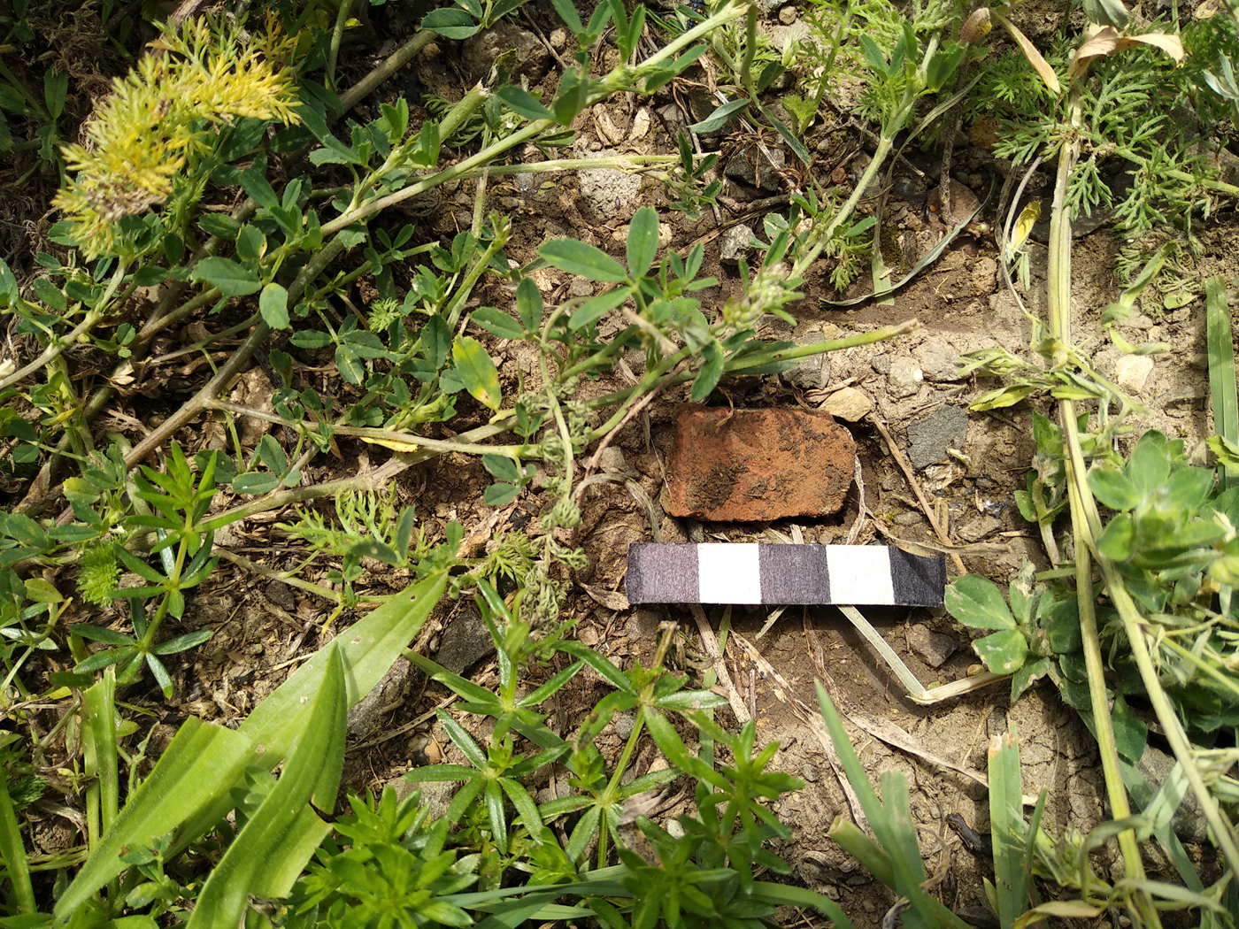
Ceramic sherd with scale bar, photographed in situ using the data collection Android app.
Our app has several differences from off-the-shelf apps such as ArcGIS Collector. First, no license is required because it is open source, available for download from GitHub (github.com/anatolian). Second, it supports relational database design and development, a functionality that is practically unimplemented in ArcGIS, for example. Third, the app directly communicates with the Reach rover to read coordinates and coordinate quality. Finally, we designed it to collect archaeological survey data, and we are continuing to improve efficiency for this specific use (similar to the custom app of Cascalheira et al. Reference Cascalheira, Bicho and Gonçalves2017).
University of Pennsylvania software engineering students developed the Android app over two academic semesters with funding from the Price Lab for Digital Humanities. One of these programmers came to Armenia, along with a new student programmer. The software developers, therefore, had the opportunity to refine the app based on direct experience. The software consists of both the Android app and a Python web service that enables communication with the project's cloud-based database.
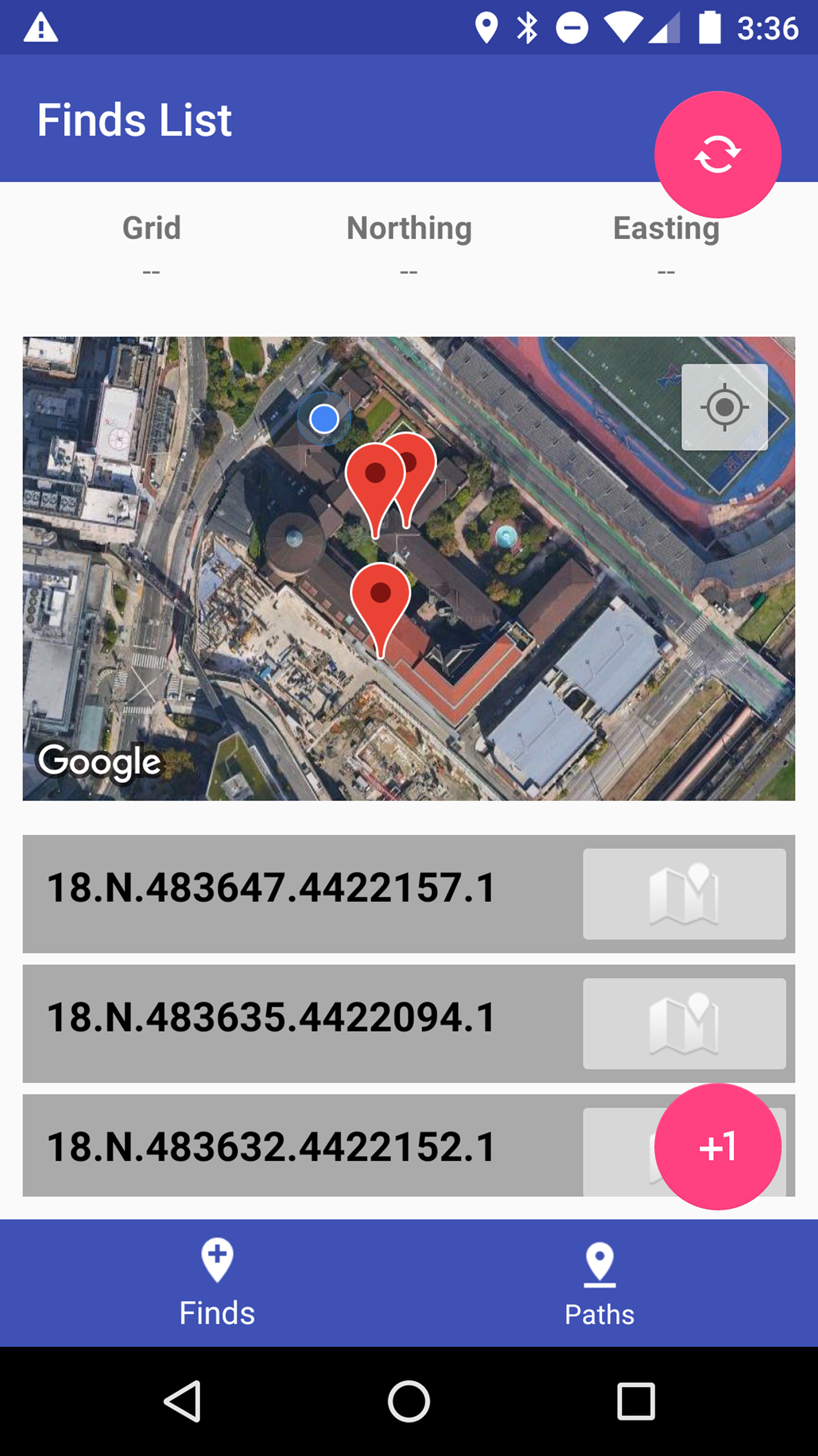
A streamlined user interface simplifies the app's use and development. The two main pages are for finds and tracks. The app opens to the Finds home page by default, which displays a map and a list of the points collected (Figure 5). Above the map is the user's current location in Universal Transverse Mercator (UTM) for guiding the maintenance of northing or easting in a straight-line survey. For this feature, we plan to eventually replace the low-accuracy phone GNSS position with a Reach RS position.
Android screenshot of the Finds home page, with a map and list of finds identified by UTM coordinates.
The workflow for entering a new find was designed for efficiency and ease of use. The plus button at the bottom of the screen opens the Finds entry page so one can add a new find (Figure 6). This page displays a live update of the current position and indicates its source and quality. The user, once satisfied with the position reading, hits the “updating” button to fix the point in memory (the button text then changes to “fixed”). Pressing the button once more causes the position to update again, when needed to reset the point. Buttons for taking photographs or loading photographs from the Android device's memory (gallery) are located below the position information, along with fields for an object's material class and free-form notes. This screen implements our goal of recording fundamental aspects of a field find quickly, but it can be customized to fit other recording strategies.
Android screenshot for recording a find.

The Tracks feature of the app records where field walkers have searched for evidence, allowing us to account for the absence of remains; the Tracks home page, like the Finds home page, presents a map and tracks list. Our initial implementation was simple: we recorded only the start and end points of each track, assuming each line to be perfectly straight (Figure 7). The complex topography in this region, however, prevented us from testing this functionality because most of our tracks were not straight lines. Therefore, we relied instead on an off-the-shelf track recording app called Map My Walk. This app recorded only at the accuracy of the device's internal GNSS receiver, capturing points every 10 m. If every team member carried a Reach RS rover, the tracks would be more accurate. The app saved tracks to a website, downloadable as .gpx files for importation into ArcGIS or Quantum GIS (QGIS), an open-source GIS software package that we plan to use in the future. We visualized where each person walked each day to indicate what parts of the landscape we sampled.
Android screenshot for recording a straight-line track by capturing start and end points.

A stable Internet connection was key to our workflow, because the Reach base lacked a long-range radio and the Reach RS rover needs a continuous connection to the base to receive corrections. Each field walker who carried a rover had an Android device that both ran the app and served as an Internet hot spot for the rover. Although continuous Internet did make it possible to upload data immediately to the cloud database, we preferred uploading data at our field house at day's end. We focused on data recording in the field and worried about data upload when we had fewer distractions.
We experimented with several techniques for uploading the data and photographs to our virtual desktop server (VDS). Ultimately, our goal was to transfer the data to our postgresql database and the photographs to the hard drive of our VDS, which centralized our dataset in the cloud. Our app uploaded database information via a Web service, a set of websites that can accept posts of structured data. The Web service, written in Python, then transferred the data to a cloud-based postgresql database. Although we preferred to run the Web service and database on our VDS, firewall restrictions prevented us from doing so. Instead, we used the free-tier cloud hosting of an Amazon Web Services database and a Heroku Python Web server. The VDS connected to the same cloud database, enabling us to display and manipulate data through multiple interfaces, including Microsoft Access forms, ArcGIS, and QGIS. We experimented with multiple cloud services for uploading photographs, but found it easiest to automatically organize the photographs on the Android device's storage and then manually copy them to the VDS. We plan to implement direct uploads in a future season. Given our 4G mobile data connection at our field house, we had no problem moving all the data to the cloud and then querying and manipulating it over the virtual desktops.
Measurement Quality Testing
To test the consistency of the Reach's geographical measurements, we established a pair of test points 25 m from each other and 1 km from the base (1 km baseline). Over the course of one week, we used the rover on several days, recording each point twice to test the precision across both short and long time scales (Table 1). We calculated the precision of these recorded measurements using standard distance (in earth-centered, earth-fixed coordinates), which is conventional for GIS analysis (Mitchel Reference Mitchel2005). To test potential limits in the precision of altitude measurements with the L1 GNSS frequency, we calculated the standard distance of XY and Z separately and then XYZ combined. We observed that Point 1 had a standard distance that is higher in XY but lower in Z than Point 2 (Table 2; Figure 8). Although adding in the Z measurements increased the standard distance of both points, it did so by less than 0.5 cm in both cases. Additionally, both points had a full XYZ standard distance of less than 2 cm, making the measurements more than adequate for the surface survey. With additional testing and a more stable base, the system should be satisfactory for excavation. We recommend that teams measure known test points each day to verify that the device is operating correctly and that no new issues have been introduced.

Test Point Measurements.

aAR Ratio measures the quality of the differential – anything above 3 results in a fixed measurement.
bXYZ coordinates are recorded in the Earth Centered Earth Fixed (ECEF) system as meters.
Test Point Error Calculation.

aXYZ coordinates are recorded in the Earth Centered Earth Fixed (ECEF) system as meters.
bStandard distance, in centimeters, calculated using the specified subsets of coordinates.
RESULTS
Our team of six field walkers employed the app throughout the season. To achieve our research goals of equipment and software experimentation, we made important changes to our system, especially during the first third of our season. This type of reflexive technical development is common for early-stage software and hardware implementations. In particular, we went through multiple iterations of the workflow for uploading data to the cloud. It also took several field days to establish a reliable configuration for the dGNSS base. Ultimately, we were able to record all field data using the app and to collect many of our find points with the dGNSS. Thus, even in this first season, the overall performance of our recording system was satisfactory, and our building and learning efforts position us well for subsequent field seasons.
Our team walked a combined total of approximately 240 km. Assuming a 2 m buffer around each field walker, this resulted in a total area investigated of approximately 48 ha. We recorded a total of 430 find points in the field for an overall find density of about 9 finds per hectare. Our finds included mostly ceramic sherds, lithics, and stone architectural features. We collected 135 ceramic and lithic samples for further analysis and documentation. The low density of surface finds provided a suitable environment for experimentation with archaeological recording technology because we were not overwhelmed by data collection during field walking.
The single Reach RS rover was our main limitation, which can be remediable in future seasons by bringing multiple units. Often, we were able to run the rover to each field walker who found an object. Some days, however, the field walkers were too far apart or the finds were too dense to make this practical. When the Reach RS was not available, the Android device's own low-accuracy GNSS device would provide the point instead. Across the full dataset, 38.6% (n = 166) of points were recorded using only the internal Android GNSS. Of the points recorded with the dGNSS system, 65% (n = 171) were recorded with a fixed signal, with the remainder on float (n = 77) or single (n = 16).
Intensive Survey
High-precision locational recording of individual finds opens new possibilities for the investigation of intra-site space. Documenting every find on a site covered by a dense scatter of artifacts requires a significant increase in the efficiency of data acquisition. Precise position information is an absolute necessity when finds are deposited only centimeters apart. We see multiple research potentials for this type of recording, from mapping exact site surface extents to plotting ceramic shape distribution that may inform us about differential uses of space.
We applied our digital recording workflow to the intensive systematic survey of a known site: a relatively flat site northeast of modern Karaglukh that was probably a medieval village. A ravine on the south side and a ridge to the northwest define the site: this circumscribed topography lent itself to a contained systematic surface survey. Our goal was to use the Reach RS on a fixed signal to precisely establish our survey intervals and record all finds. With 5 m interval tracks, GNSS precision has a major influence on results. We attempted to maintain strict east–west tracks while recording every find with the dGNSS. Over the course of about three hours on the morning of June 15, 2018, we recorded 101 finds, almost one-quarter of the season's total. Because all points were recorded on a fixed signal, we could precisely map finds from this small portion of the site.
Use of a single dGNSS rover limited us in two ways. First, field walkers were not able to maintain strict east–west lines. Our app displays the UTM coordinate to facilitate straight walking; however, the Android device's internal GNSS position was not accurate enough to maintain the Reach-established line. Future improvement efforts will involve integrating the dGNSS signal into the real-time app display. The second bottleneck was that only the person with the dGNSS rover could set start and end tracks and record finds, which required that individual to move around a great deal. An obvious solution to both problems would be equipping each field walker with a dGNSS rover. This experiment did allow us to test the Tracks recording screen of our app, which records start and end points for straight-line tracks.
Remaining Challenges
We made significant progress in demonstrating the system's field worthiness. Several issues remain, and we plan to make improvements for next season. Perhaps the greatest challenge is implementing the system in an area with denser material remains. An increase in the number of finds could slow down a field walker, preventing the group from maintaining a coordinated pace, which has both safety and social implications. Where conditions allow, the app could eventually guide field walkers to avoid areas already examined by fellow field walkers, preventing redundant recording. Another challenge is maintaining the photographic component of the recording system while improving workflow efficiency. One of the most time-consuming aspects was placing a centimeter scale bar next to the find before it was photographed. We hope to develop a system—perhaps placing the bar at the end of a pole—to more quickly and easily include the scale bar and add a color standard in each photograph.
The dGNSS configuration we deployed in the field functioned well for our application; however, the initial setup required experience, patience, and maintenance. One challenge for wide adoption would be ensuring satellite signal reception for the Reach circuit board. Luckily, in the clear skies and high altitude of rural Armenia, the signal was strong and relatively reliable.Footnote 1 We suggest that field performance would be improved by using a prepackaged Reach RS+ unit instead as the base and not using the Reach circuit board product, even though its cost is significantly lower. Perhaps a later iteration of the product, such as the Reach M+, will make this a more suitable option. An attempt to bring another Reach RS+ into the field highlighted the challenges of deploying cutting-edge technology, as repeated shipping delays meant that the second unit would have arrived only at the end of our season.
Achieving the research goal of efficiency depends on consistent fixed measurements from the dGNSS equipment, which are difficult to acquire during a highly mobile survey. Because the rover was being moved around, it was not always pointed toward the sky. Thus, when we stopped, we had to wait a few seconds or even a minute for the device to receive satellite signals and get to a fixed status. When it became stuck on float, moving the device a few dozen meters away and then back to the target position would reset the device to a fixed status. Another challenge was the Internet connection. Although the base had a constant Internet uplink after we implemented our stable setup, the field team moved through areas lacking consistent mobile service. Given the remote and rural character of the valleys, however, we were pleasantly surprised that we did have 3G or 4G signals most of the time.
Finally, to remain as mobile as possible, we chose not to carry a surveying rod. Thus we often recorded positional information above the actual ground-level find. One way to solve this problem in future seasons and allow for hands-free operation is to have each field walker carry a rover on a backpack at a known height.
CONCLUSION
Our experiences with this dGNSS setup indicate that affordable dGNSS will soon be available to most archaeological projects and be able to function well in typical fieldwork operational environments. In future seasons we will refine our workflow by provisioning each field walker with a rover and using a more stable device as the base station. At that point, the dGNSS technology will move into the background as we focus our time on research questions about the landscapes. Furthermore, most specific problems we encountered during the 2018 fieldwork arose from the constraints of conducting a mobile surface survey. The static situation of an excavation would enable easier deployment, particularly in areas with excellent satellite visibility. Differential GNSS systems are not limited solely to the use described in this article or to excavations but are applicable to many archaeological methods. The adaptation of technology to archaeology is ultimately a function of its cost and ease of use.
Archaeological fieldwork relies increasingly on the interpretation of digitally captured and curated datasets, so we should strive to implement methods that improve the quality of the data we collect (Roosevelt et al. Reference Roosevelt, Cobb, Moss, Olson and Ünlüsoy2015). The need to improve data quality, especially spatial data, is highlighted by open-source initiatives that seek to facilitate comparative and big data projects (Kansa Reference Kansa2012; McManamon et al. Reference McManamon, Kintigh, Ellison and Brin2017; Marwick and Birch Reference Marwick and Pilaar Birch2018). Steps to support the reproducibility of our results underpin the open approach to archaeology (Huggett Reference Huggett2018; Marwick et al. Reference Marwick, d'Alpoim Guedes, Barton, Bates, Baxter and Bevan2017). Global heritage faces many risks that motivate us to preserve archaeological data in the most complete manner possible, a goal both worthwhile and achievable.
Acknowledgments
The Price Lab for Digital Humanities at the University of Pennsylvania provided support for hardware and the student programmers. The Penn Museum of the University of Pennsylvania supported the archaeological survey in Armenia and the travel of the engineering students. We are particularly grateful to our Armenian codirectors, Artur Petrosyan and Boris Gasparyan, from the Institute of Archaeology and Ethnography at the National Academy of Sciences of Armenia. The regional survey was authorized under the 2018 Armenian Ministry of Culture Permit No. 03/14.2/3310-18. We thank Anvith Ekkati, Christopher Besser, and Colin Roberts for programming efforts; Dr. Laura Piedra Muñoz for helping with our abstract; Kyle Kern for assisting with the references; and Penn's Center for the Analysis of Archaeological Materials.
Data Availability Statement
This article reported no original data.


 Open access