


Impact statement
Underwater 3D scanning systems are pivotal in fields such as marine archaeology, offshore engineering, and environmental monitoring. Such systems provide critical insights for applications ranging from seafloor mapping to infrastructure inspection. However, conventional scanning methods are often hindered by slow data acquisition and inefficiencies. This research addresses these limitations by introducing a low cost, AI-driven scanning approach that enhances the speed, accuracy, and efficiency of underwater surface mapping. The new scanning method, which integrates Bayesian optimization and Gaussian Process regression, reduces the time required to visualize surfaces by intelligently selecting measurement locations that maximize information gain. Laboratory tests demonstrate that this approach generates precise surface models with a fraction of the data and time required by conventional methods. This advancement has broad applicability and significant impact across disciplines. In industry, it enables real-time monitoring of critical infrastructure, such as offshore wind turbine foundations, reducing risks and operational downtime. For government and environmental agencies, the method offers a rapid and accurate solution for tracking erosion, sediment transport, and other dynamic processes. In academia, it provides a robust framework for future innovations in underwater robotics and geospatial analysis.
1. Introduction
Underwater scanning systems are widely employed across diverse fields, including marine archaeology (Menna et al., Reference Menna, Agrafiotis and Georgopoulos2018; Bräuer-Burchardt et al., Reference Bräuer-Burchardt, Munkelt, Bleier, Heinze, Gebhart, Kühmstedt and Notni2023), offshore engineering (Palomer et al., Reference Palomer, Ridao and Ribas2019; Chemisky et al., Reference Chemisky, Menna, Nocerino and Drap2021; Sun et al., Reference Sun, Cui and Chen2021), and underwater robotics (Chutia et al., Reference Chutia, Kakoty and Deka2017; Cong et al., Reference Cong, Gu, Zhang and Gao2021). These systems enable the measurement and visualization of critical areas of interest. Despite their utility, there remains significant scope for improving the performance and efficiency of current underwater scanning technologies.
Unlike their counterparts used in air, underwater scanners often require extended periods to acquire measurements due to the challenging conditions of submerged environments (Menna et al., Reference Menna, Agrafiotis and Georgopoulos2018). Most existing dual-axis scanning systems follow a concentric circular pattern, which is time-intensive and involves capturing numerous redundant measurements with minimal additional informational value (Clarke, Reference Clarke2009). While reducing the number of measurements could shorten scanning times, indiscriminately changing the scanning pattern risks missing critical surface features. Therefore, a key challenge lies in determining optimal measurement locations.
Rapid data acquisition is important for autonomous systems, such as underwater robots, which are limited by their finite battery life (Chutia et al., Reference Chutia, Kakoty and Deka2017; Cong et al., Reference Cong, Gu, Zhang and Gao2021). It is also critical for dynamic underwater applications where conditions change quickly, such as monitoring scour (Lind and Whitehouse, Reference Lind and Whitehouse2012), which is critical for the maintenance of offshore monopile foundations (Byrne et al., Reference Byrne, Aghakouchak, Buckley, Burd, Gengenbach, Houlsby, McAdam, Martin, Schranz, Sheil and Suryasentana2020). It is also essential for monitoring the installation of offshore foundations. Rapid scanning is required to capture fast-evolving seabed changes during the installation of suction caisson foundations (Sparrevik and Strout, Reference Sparrevik, Strout and Meyer2015), which are increasingly used for offshore wind applications (e.g., Suryasentana et al., Reference Suryasentana, Byrne, Burd and Shonberg2018, Reference Suryasentana, Burd, Byrne and Shonberg2023a, Reference Suryasentana, Burd, Byrne and Shonberg2023b, Reference Suryasentana, Sheil and Stuyts2024).
This paper addresses this challenge by introducing a novel Artificial Intelligence (AI)-driven scanning approach. This approach is designed to address the inefficiencies of traditional techniques and aligns with the growing adoption of AI to transform offshore geotechnical practices (Stuyts and Suryasentana, Reference Stuyts and Suryasentana2023). The approach utilizes probabilistic machine learning techniques, including Bayesian optimization and Gaussian Process (GP) regression. The Bayesian optimization algorithm selects the most informative locations for measurements, significantly reducing the number required for a scan (Shahriari et al., Reference Shahriari, Swersky, Wang, Adams and de Freitas2016). GP regression predicts the surface geometry based on sparse measurement data, effectively filling in gaps and further minimizing the effort needed for data acquisition (Rasmussen and Williams, Reference Rasmussen and Williams2008). This paper outlines the operational principles of current underwater scanning technologies and describes the implementation of the proposed AI-driven scanning system. It covers the hardware and software design and development of a prototype three-dimensional scanning device, along with the integration of Bayesian optimization and GP regression algorithms that control the scanning process. The prototype was developed and tested in ideal laboratory conditions that mimicked those found in offshore deployment.
This paper presents two key novel contributions. First, it introduces an innovative, low-cost AI-driven approach to underwater 3D scanning based on Bayesian optimization, 3D printing and single-beam echosounders. This approach is more cost-effective than comparable commercially available devices and allows for faster and more accurate surface geometry estimation, enabling the system to adapt to a variety of surface types without relying on predefined scanning patterns. The system dynamically adjusts its scanning strategy based on real-time surface characteristics, autonomously optimizing the data collection process. Second, the paper demonstrates the practical application of this approach by developing and testing a prototype of the AI-driven underwater scanning system in controlled laboratory conditions. Experimental results show that the system can accurately model different surface geometries with fewer measurements, leading to significant reductions in scanning time, data storage, and processing requirements. Together, these contributions represent a significant advancement in underwater scanning technology, improving its efficiency, adaptability, and accuracy.
2. Methodology
2.1. Existing underwater measurement technology
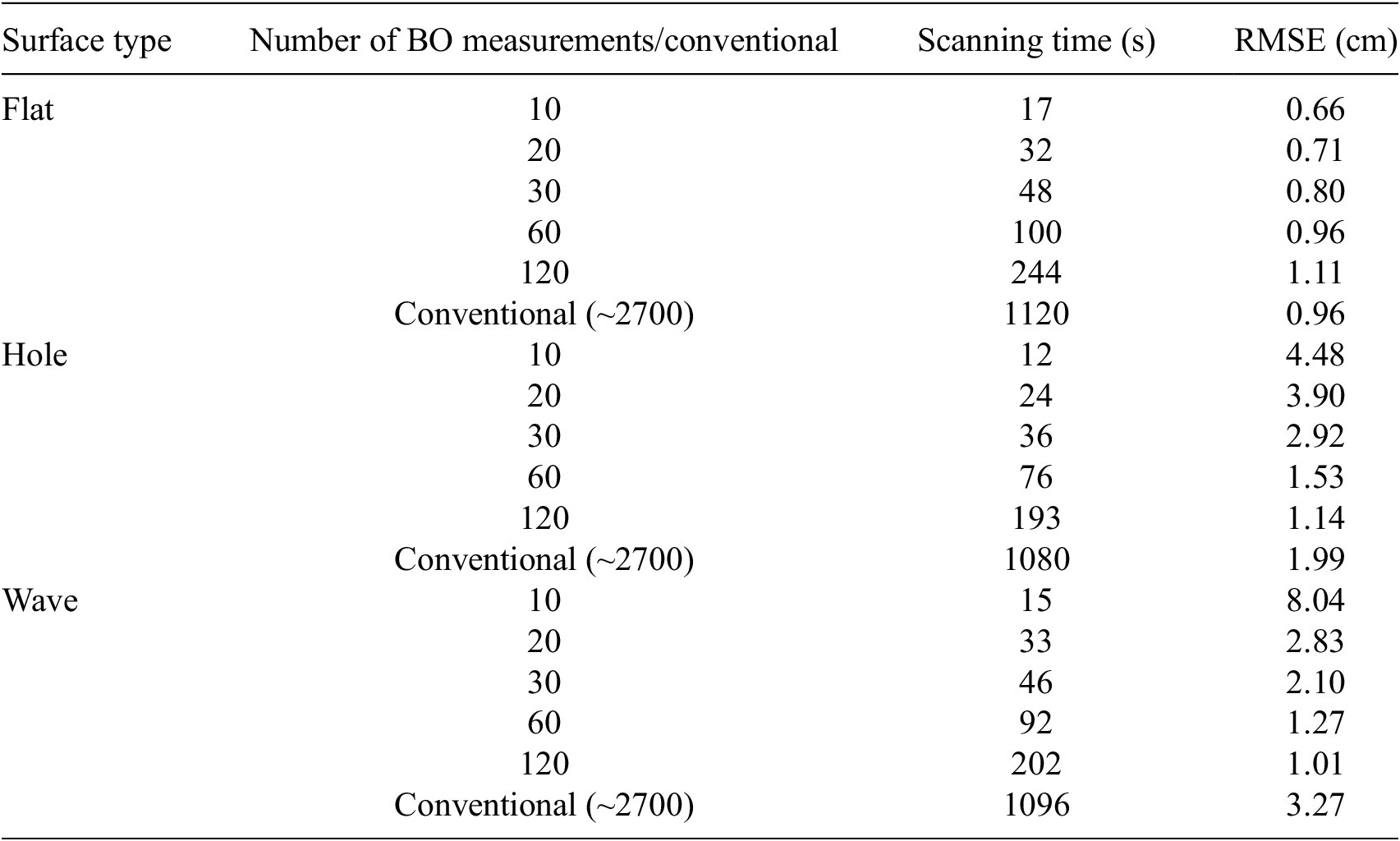
Most underwater 3D scanners use either ultrasound or lasers, applying either time-of-flight or triangulation principles to acquire measurements (Massot-Campos and Oliver-Codina, Reference Massot-Campos and Oliver-Codina2015). In time-of-flight devices, a pulse is emitted and reflected off a surface. By measuring the time it takes for the pulse to travel from the emitter to the surface and back, and knowing the speed of the signal in the medium, the distance to the surface can be calculated (Lurton, Reference Lurton2002; Massot-Campos and Oliver-Codina, Reference Massot-Campos and Oliver-Codina2015). Triangulation, on the other hand, uses the known angles and distances between surveying points to calculate the distance to a target. In laser-based systems, these points typically include the laser (emitter), a camera (receiver), and a known feature or target on the camera image (Massot-Campos and Oliver-Codina, Reference Massot-Campos and Oliver-Codina2015).
In offshore settings, ultrasound measuring devices are the most commonly used and have demonstrated reliability over many years (Coates, Reference Coates1990; Lurton, Reference Lurton2002). The most cost-effective of these devices is the single-beam echosounder, which uses the time-of-flight principle to acquire measurements. Despite certain limitations, single-beam echosounders are widely used in the offshore industry due to their ability to provide accurate measurements over long distances and operate effectively in turbid water and harsh environmental conditions (Coates, Reference Coates1990; Lurton, Reference Lurton2002). Multi-beam echosounders, which consist of an array of single-beam echosounders arranged in a fan pattern, can collect 3D data more rapidly. However, they tend to be bulky, expensive, and prone to signal interference when used in confined spaces or shallow waters, which can result in inaccurate measurements. Consequently, multi-beam echosounders are primarily used for bathymetric data collection (Lurton, Reference Lurton2002). A more economical underwater device for capturing 3D data is the dual-axis mechanical scanning sonar. This system uses two stepper motors to move a single-beam echosounder along two axes to record measurements. By tracking the angles of the motors and the distance measured by the echosounder, the system can generate 3D coordinates. These coordinates are then used to create a point cloud, which visualizes the underwater scene (Clarke, Reference Clarke2009).
Laser distance measurement devices are becoming increasingly popular for underwater inspections, but are still less commonly used than ultrasound devices. They offer distinct advantages, such as faster measurement acquisition and superior spatial resolution compared to ultrasound (Massot-Campos and Oliver-Codina, Reference Massot-Campos and Oliver-Codina2015). Additionally, unlike ultrasound, laser devices are not affected by interference from residual signals (Chemisky et al., Reference Chemisky, Menna, Nocerino and Drap2021). However, their performance is significantly influenced by water’s physical properties (Menna et al., Reference Menna, Agrafiotis and Georgopoulos2018). For example, complex calibration is needed to address refraction at the water-lens interface (Chemisky et al., Reference Chemisky, Menna, Nocerino and Drap2021). Their operational range is limited because laser light is strongly attenuated in water. Moreover, in turbid conditions, scattering from suspended particles further reduces their effective range (Menna et al., Reference Menna, Agrafiotis and Georgopoulos2018). Therefore, their maximum range is significantly lower than that of ultrasound devices. Most underwater laser distance measurement devices belong to two main types: (i) Laser line scanners with triangulation, or (ii) Light Detection and Ranging (LIDAR) devices. Laser line scanners project a laser line onto a surface and use cameras to capture its deformation, enabling the creation of very detailed 3D profiles in a short period of time. These devices are particularly suited for close-range inspections and high-resolution imaging. LIDAR systems, on the other hand, emit pulsed laser beams and calculate distances by measuring the time-of-flight of the reflected light. A summary of the different types of commercially available ultrasound and laser scanners and their characteristics is provided in Table 1.
Commercially available underwater scanners and their typical characteristics

2.2. Bayesian optimization
Bayesian Optimization (BO) is a widely used machine learning method for finding the maximum of an unknown, expensive-to-evaluate objective function g(x), which takes the form:
 $$ {x}^{\ast }={\mathrm{argmax}}_x\;g(x) $$
BO has been applied successfully across various domains, including environmental monitoring (Marchant and Ramos, Reference Marchant and Ramos2012), optimization of machine learning model hyperparameters (Wu et al., Reference Wu, Chen, Zhang, Xiong, Lei and Deng2019) and physical devices like lasers (Jalas et al., Reference Jalas, Kirchen, Messner, Winkler, Hübner, Dirkwinkel, Schnepp, Lehe and Maier2021), as well as robot control (Martinez-Cantin, Reference Martinez-Cantin2017). A key strength of BO is its efficiency in minimizing the number of function evaluations required to characterize the objective function (Shahriari et al., Reference Shahriari, Swersky, Wang, Adams and de Freitas2016). This efficiency is achieved by incorporating prior knowledge to strategically select sampling locations. BO balances the trade-off between exploration, which involves sampling areas with high uncertainty, and exploitation, which targets areas where the objective function is expected to be high. When applied to the control of a 3D scanner, BO aims to minimize the number of measurements required to characterize a target surface. This approach significantly reduces the time needed to make reliable predictions of the surface.
BO operates through a series of iterative steps. First, a surrogate model is created to approximate the objective function, with GP regression commonly used for this purpose (Shahriari et al., Reference Shahriari, Swersky, Wang, Adams and de Freitas2016). Next, an acquisition function is employed to decide the most promising location to sample the objective function. The acquisition function leverages the surrogate model’s predictions to identify the point where the objective function is likely to be at its maximum. The objective function is then evaluated at this selected location, and the resulting data is used to update the surrogate model. This process of updating the model and selecting new sampling points continues iteratively until the optimization goal is achieved.
When applying BO to problems where there is a tangible time cost associated with moving to new sampling points (e.g., in physical systems where a device must physically travel to a sampling location, unlike computational simulations where movement costs are negligible), it may be necessary to use a specialized acquisition function that accounts for these costs. Such a function balances the need to select informative points with the need to minimize delays caused by traveling to distant sampling locations. Marchant and Ramos (Reference Marchant and Ramos2012) proposed the distance-based upper confidence bound (DUCB) function to address this issue. This acquisition function incorporates a distance penalty to priorities closer sampling points and reduce delays in data acquisition.
In the current study, the aim is to reconstruct unknown target surfaces with different geometries by strategically selecting sampling locations that maximize information gain. GP regression serves as the surrogate model for the unknown target surface elevations with respect to the sensor location, providing both predictions of the surface shape and estimates of uncertainty. To achieve this aim, the following acquisition function is employed, which selects the next sampling location
 $ {x}^{\ast } $
as the location with maximum uncertainty:
$ {x}^{\ast } $
as the location with maximum uncertainty:
 $$ {x}^{\ast }={\mathrm{argmax}}_x\;\sigma (x) $$
where
 $ \sigma (x) $
is the GP’s posterior standard deviation at location
$ \sigma (x) $
is the GP’s posterior standard deviation at location
 $ x $
. The acquisition function used in this study does not include a distance penalty (Marchant and Ramos, Reference Marchant and Ramos2012), as initial experiments revealed that selecting distant locations incurs minimal additional cost compared to nearby ones. The values of
$ x $
. The acquisition function used in this study does not include a distance penalty (Marchant and Ramos, Reference Marchant and Ramos2012), as initial experiments revealed that selecting distant locations incurs minimal additional cost compared to nearby ones. The values of
 $ \sigma (x) $
are influenced by the geometry of the target surface; simpler geometries result in lower
$ \sigma (x) $
are influenced by the geometry of the target surface; simpler geometries result in lower
 $ \sigma (x) $
values with few observations, compared to more complex geometries. By targeting regions of high predictive uncertainty, this acquisition function ensures efficient exploration of the domain, leading to improved surface reconstruction with minimal samples. The iterative process of updating the GP model with newly acquired measurements facilitates accurate surface estimation while avoiding unnecessary redundancy in sampled data.
$ \sigma (x) $
values with few observations, compared to more complex geometries. By targeting regions of high predictive uncertainty, this acquisition function ensures efficient exploration of the domain, leading to improved surface reconstruction with minimal samples. The iterative process of updating the GP model with newly acquired measurements facilitates accurate surface estimation while avoiding unnecessary redundancy in sampled data.
2.3. Gaussian process regression
Gaussian process (GP) regression is a probabilistic machine learning method used for non-linear regression and interpolation. It is widely used due to its flexibility in modeling complex relationships, ability to handle small datasets, and capability to provide uncertainty estimates (Suryasentana and Sheil, Reference Suryasentana and Sheil2023). A detailed explanation of GP regression can be found in Rasmussen and Williams (Reference Rasmussen and Williams2008) and Murphy (Reference Murphy2012). However, a brief explanation of the underlying theory is provided here. GP regression models an unknown function as a GP, which is a set of random variables where any finite subset has a joint Gaussian distribution. GPs can be described as a probability distribution over functions and are fully characterized by their mean function
 $ m(x) $
and covariance function (also known as the kernel)
$ m(x) $
and covariance function (also known as the kernel)
 $ k\left(x,{x}^{\prime}\right) $
:
$ k\left(x,{x}^{\prime}\right) $
:
 $$ f(x)\sim GP\Big(m(x),k\left(x,{x}^{\prime}\right) $$
where
 $ m(x) $
and
$ m(x) $
and
 $ k\left(x,{x}^{\prime}\right) $
are:
$ k\left(x,{x}^{\prime}\right) $
are:
 $$ m(x)=\unicode{x1D53C}\left[\;f(x)\right] $$
 $$ k\left(x,{x}^{\prime}\right)=\unicode{x1D53C}\left[\;\left(f(x)-m(x)\right){\left(f\left({x}^{\prime}\right)-m\left({x}^{\prime}\right)\right)}^T\right] $$
 $ m(x) $
represents the expected value of the function at input
$ m(x) $
represents the expected value of the function at input
 $ x $
, while
$ x $
, while
 $ k\left(x,{x}^{\prime}\right) $
encodes the similarity between the outputs at
$ k\left(x,{x}^{\prime}\right) $
encodes the similarity between the outputs at
 $ x $
and
$ x $
and
 $ {x}^{\prime } $
. Commonly used kernels include the Matérn kernel
$ {x}^{\prime } $
. Commonly used kernels include the Matérn kernel
 $ {\kappa}_{MA} $
and squared exponential kernel
$ {\kappa}_{MA} $
and squared exponential kernel
 $ {\kappa}_{SE} $
:
$ {\kappa}_{SE} $
:
 $$ {\kappa}_{MA}\left(x-{x}^{\prime}\right)={\sigma}^2\frac{2^{1-\upsilon }}{\Gamma \left(\upsilon \right)}{\left(\sqrt{2\upsilon}\frac{\left(x-{x}^{\prime}\right)}{\rho}\right)}^{\upsilon }{\mathcal{R}}_{\upsilon}\left(\sqrt{2\upsilon}\frac{\left(x-{x}^{\prime}\right)}{\rho}\right) $$
 $$ {\kappa}_{SE}={\theta}_f^2\exp \left(-\frac{1}{l^2}{\left\Vert x-{x}^{\prime}\right\Vert}^2\right) $$
The squared exponential kernel assumes that the functions are smooth and is therefore well suited for modelling smooth surfaces, whereas the Matérn kernel can model less smooth functions and may be better suited to modelling physical phenomena (Stein, Reference Stein2012). The values of the kernel hyperparameters, such as
 $ {\sigma}_f^2 $
and
$ {\sigma}_f^2 $
and
 $ l $
in Equation 7, are optimized by maximizing the marginal log likelihood of the observed (training) data, given the hyperparameters (Rasmussen and Williams, Reference Rasmussen and Williams2008). In the current study, the squared exponential kernel was used in the surrogate model within the BO process and to predict the target surface.
$ l $
in Equation 7, are optimized by maximizing the marginal log likelihood of the observed (training) data, given the hyperparameters (Rasmussen and Williams, Reference Rasmussen and Williams2008). In the current study, the squared exponential kernel was used in the surrogate model within the BO process and to predict the target surface.
The prior distribution of the function is a Gaussian distribution, denoted as:
 $$ f\sim N\left(f|\boldsymbol{\mu}, \boldsymbol{K}\right) $$
where
 $ {K}_{i,j}=k\left({x}_i,{x}_j\right) $
and
$ {K}_{i,j}=k\left({x}_i,{x}_j\right) $
and
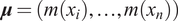 $ \boldsymbol{\mu} =\left(m\left({x}_i\right),\dots, m\left({x}_n\right)\right) $
.
$ \boldsymbol{\mu} =\left(m\left({x}_i\right),\dots, m\left({x}_n\right)\right) $
.
Once trained, the method provides not only predictions at new inputs but also an estimate of uncertainty in these predictions, making it particularly useful in applications where uncertainty quantification is important. Suppose that some observations
 $ \boldsymbol{y}={\left[{y}_1,\dots, {y}_N\right]}^T $
have been obtained for some inputs
$ \boldsymbol{y}={\left[{y}_1,\dots, {y}_N\right]}^T $
have been obtained for some inputs
 $ \boldsymbol{x}={\left[{x}_1,\dots, {x}_N\right]}^T $
and the kernel’s hyperparameters have been learnt from the training process. To predict the output
$ \boldsymbol{x}={\left[{x}_1,\dots, {x}_N\right]}^T $
and the kernel’s hyperparameters have been learnt from the training process. To predict the output
 $ {\hat{y}}_{\ast } $
for a new input
$ {\hat{y}}_{\ast } $
for a new input
 $ {x}_{\ast } $
, the GP regression model computes the conditional distribution, which is obtained analytically using the standard conditioning rules for the multivariate Gaussian distribution:
$ {x}_{\ast } $
, the GP regression model computes the conditional distribution, which is obtained analytically using the standard conditioning rules for the multivariate Gaussian distribution:
 $$ p\left(\;{\hat{y}}_{\ast }|{x}_{\ast },\boldsymbol{x},\boldsymbol{y}\right)=N\left({\mu}_{\ast },{k}_{\ast}\right) $$
where
 $$ {\mu}_{\ast }=m\left({x}_{\ast}\right)+{{\boldsymbol{k}}_{\ast}}^T{\boldsymbol{K}}^{-1}\left(\mathbf{y}-m\left(\boldsymbol{x}\right)\right) $$
 $$ {k}_{\ast }=k\left({x}_{\ast },{x}_{\ast}\right)-{{\boldsymbol{k}}_{\ast}}^T{\boldsymbol{K}}^{-1}{\boldsymbol{k}}_{\ast} $$
 $$ {\boldsymbol{k}}_{\ast}={\left[k\left({x}_1,{x}_{\ast}\right),\dots, k\left({x}_N,{x}_{\ast}\right)\right]}^T $$
 $$ \boldsymbol{K}=\mathrm{covariance}\ \mathrm{matrix},{K}_{ij}=k\left({x}_i,{x}_j\right) $$
The prediction
 $ {\hat{y}}_{\ast } $
is a weighted sum of the observed data, where the weights are determined by the trained kernel.
$ {\hat{y}}_{\ast } $
is a weighted sum of the observed data, where the weights are determined by the trained kernel.
2.4. Prototype 3D scanner
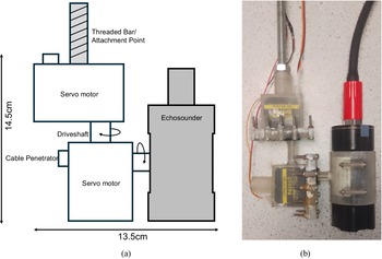
A prototype 3D scanner for the AI-driven sensor concept is constructed using a dual-axis rotating arm equipped with two 180-degree servo motors. These motors are enclosed in waterproof housings. The arm controlled a single-beam echosounder, operating at
 $ 500 kHz $
, allowing it to scan in the 3D space. An M10 threaded rod is attached to the housing to facilitate mounting of the scanner for the laboratory experiments. Figure 1 provides a schematic diagram of the scanner’s construction alongside a photo of the prototype.
$ 500 kHz $
, allowing it to scan in the 3D space. An M10 threaded rod is attached to the housing to facilitate mounting of the scanner for the laboratory experiments. Figure 1 provides a schematic diagram of the scanner’s construction alongside a photo of the prototype.
(a) Schematic diagram of the dual axis ultrasound point scanner. (b) Prototype 3D scanner.

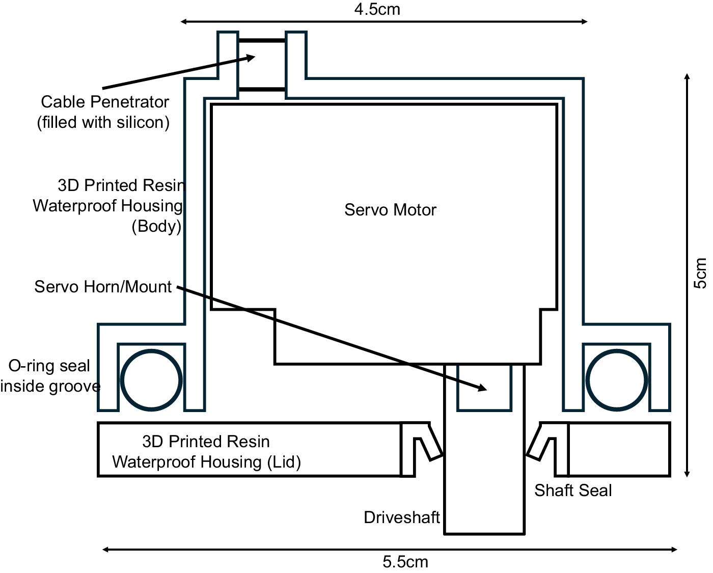
Figure 2 illustrates the construction of the waterproof housings. These housings are fabricated using thick, 3D-printed resin for durability. A rubber O-ring seated in a flange groove ensures a watertight seal at the junction between the housing lid and its main body. To maintain a waterproof barrier around the rotating driveshaft, a rubber rotary shaft seal is used. Additionally, the cables are routed through a protrusion on the housing, referred to as a cable penetrator, which is filled with silicone sealant to prevent water ingress.
Schematic diagram of the waterproof servo motor housing.

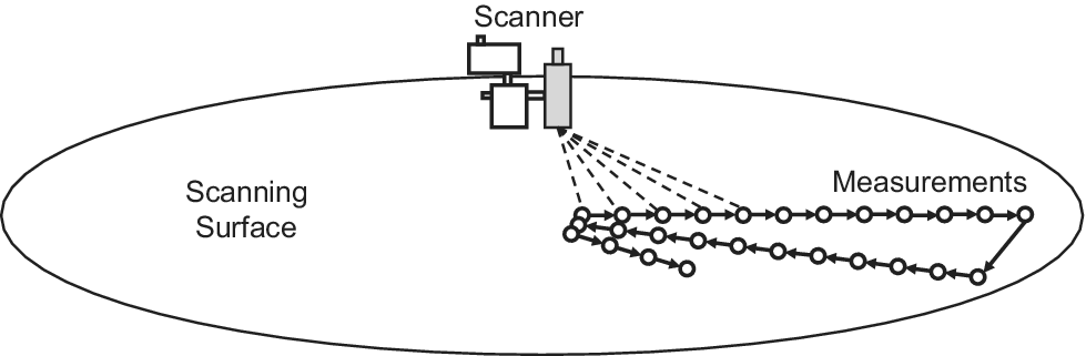
A Raspberry Pi computer controls the operation of the echosounder and servo motors. By recording the angle feedback from the servo motors and the distance measurements from the echosounder, the system calculates the spherical polar coordinates of the target surface for each measured data point. The computer contains both the BO algorithm and the conventional scanning algorithm. The conventional scanning algorithm employs a ‘brute force’ method, systematically sweeping the entire target surface with a series of line scans. During each line scan, the echosounder records measurements at every two-degree increment of the servo motor’s movement along the path. The process starts with the scanner tracing a straight line from the point beneath the echosounder to the edge of the target surface. Once this scan is completed, the scanner rotates two degrees around the vertical axis and conducts the next line scan, moving from the edge back toward the point beneath the echosounder. This alternating pattern continues, with the scanner rotating two degrees around the vertical axis after each pass, until the entire target surface has been fully scanned. Figure 3 illustrates the conventional scanning pattern.
Schematic diagram of the conventional scanning pattern.

2.5. Laboratory experiments
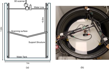
All laboratory experiments were conducted underwater in an 800 L cylindrical water tank with a height of 1.2 m and a diameter of 1 m. The experimental setup is shown in Figure 4, with the prototype 3D scanner positioned at the center of the tank cross-sectional area. The target surface was placed 50 cm below the scanner.
(a) Schematic diagram of the experimental equipment. (b) A top-down picture of the experimental equipment.

Three different target surfaces were used during the experiments, each made of 2.5 mm thick PVC and circular, with a diameter of approximately 80 cm. The first surface is perfectly flat and serves as a control to verify the proper functioning of the scanner. The second surface was shaped like a conical hole, mimicking a scour hole. The third surface took a ‘wave-like’ form, a more complex shape used to evaluate the performance of the Bayesian scanning method in areas with multiple critical zones. This wave-like surface also mimicked sediment buildup in rivers and wave imprints on the seafloor. Photos of the different target surfaces used in the experiments are shown in Figure 5.
Target surfaces used to test the 3D scanner: (a) hole surface, and (b) wave-like surface.

During the laboratory experiments, the following procedure was followed for all three surfaces. First, a full scan of the surface was conducted using the conventional scanning algorithm. This scan ensured the scanner was fully functional and provided a baseline for comparison with the BO-driven scan. Once the conventional scan was completed, the BO-driven scan was performed. As the BO-driven scan has no fixed endpoint, it was left to collect 120 measurements.
To estimate the target surface from the measurements, a GP regression model is used to predict the surface from the measurements, instead of linear interpolation, which is traditionally used. This approach allows for more reliable predictions of the shape of the surface, especially when extrapolating from the measurements. A mathematical representation for each target surface is also available as ‘ground truth’ to evaluate the accuracy of the scans.
3. Results
3.1. Flat surface (control)
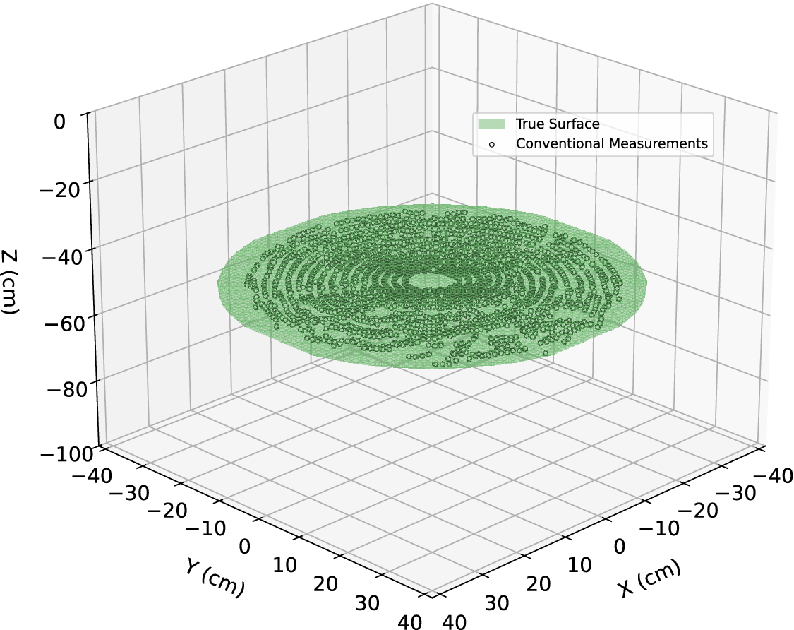
Figure 6 compares the true (mathematically derived) surface with the point cloud obtained from the measurements of the conventional scanning method. This point cloud, referred to as the “conventional surface”, closely matches the true surface, though some noise is observed in the measurements. The empty space at the center of the conventional surface is due to the echosounder being mounted off-center on the scanner. Some measurements were considered anomalous, as they deviated significantly from the others. The exact cause of these anomalies is unclear as repeated scans result in random point measurements being anomalous. These anomalous measurements were removed to minimize their impact on the RMSE evaluation, thus resulting in some minor gaps in Figure 6.
True (green) flat surface and the point cloud (white) gathered using the conventional scanning method.

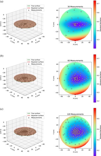
Figure 7 presents a comparison between the true flat surface and the surface predicted by the GP regression model trained on an increasing number of measurements from the BO-driven scans. The figure also shows the locations of the measurements taken during the BO-driven scans and the standard deviation of the GP-regression model, which was used as the BO acquisition function. The GP regression-predicted surface, referred to as the ‘Bayesian surface’ closely matches the true surface, with as little as 30 measurements taken. The first 30 measurements are spread evenly over the surface with a slight focus on the center. The following 30 measurements are taken in areas where the standard deviation is largest, and the final 60 measurements follow the same pattern.
3D surface plots comparing the true flat surface (green) with the GP regression-predicted surface (red) trained on the BO-driven scan measurements (white markers). 2D plots showing the location of measurements taken during the BO-driven scan from a top down view, and the heatmap of the model’s acquisition function or standard deviation. The subfigures show the surface predicted by the GP regression model trained on different number of measurements: (a) 30, (b) 60, and (c) 120.

3.2. Hole surface (Scour)
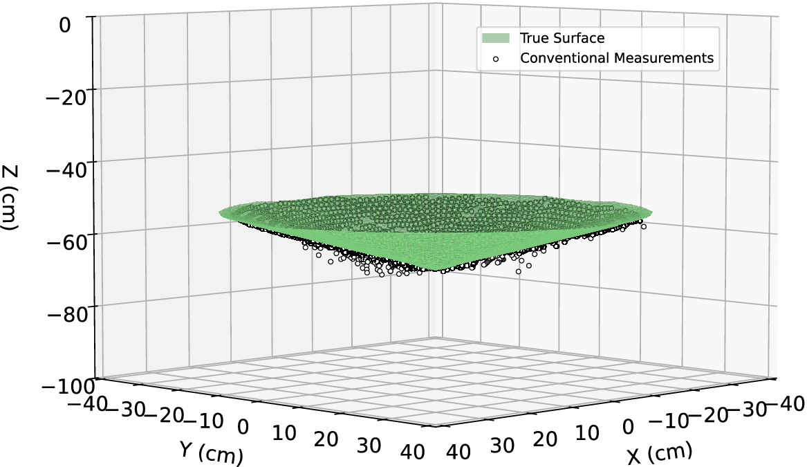
Figure 8 compares the true hole surface with the point cloud generated using the conventional scanning method. The point cloud aligns closely with the true surface, with most points positioned near the surface. As in previous analyses, some anomalous data points were excluded. Figure 9 compares the true and Bayesian hole surfaces. The Bayesian and true surfaces agree very well with each other when at least 60 measurements have been taken. Figure 9 also shows the location of the measurements taken during the BO scan, which are initially evenly spread across the surface, before covering areas where the standard deviation was greatest.
Comparison between the true (green) hole surface and the point cloud (white) gathered by the conventional scanning method.

3D surface plots comparing the true hole surface (green) with the GP regression-predicted surface (blue) trained on the BO-driven scan measurements (white markers). The subfigures show the surface predicted by the GP regression model trained on different numbers of measurements: (a) 30, (b) 60, and (c) 120.

3.2. Wave surface (seafloor)
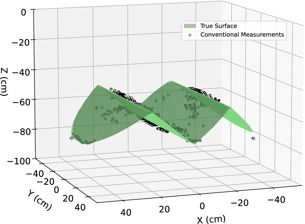
Figure 10 compares the true wave-shaped surface with the point cloud collected by the conventional scanning method. As with previous comparisons, most of the point cloud lies within an acceptable tolerance of the true surface. However, there are noticeable gaps in the point cloud at the far left- and right-hand sides. These gaps result from the removal of anomalous data. Additionally, these sides of the surface face away from the scanner, making accurate readings more difficult due to limited backscatter, which exacerbates the issue.
Comparison between the true (green) wave surface and the point cloud (white) gathered by the conventional scanning method.

Figure 11 compares the true and Bayesian wave surfaces. In Figure 11a, it is evident that there are some differences between the two surfaces on the right-hand side. The BO algorithm is highly uncertain about this area, as can be seen by the large red area on the standard deviation heatmap plot. In Figure 11b, more measurements have been taken in this area and both the standard deviation and the differences in the two surfaces have been reduced.
3D surface plots comparing the true wave surface (green) with the GP regression-predicted surface (blue) trained on the BO-driven scan measurements (white markers). The subfigures show the surface predicted by the GP regression model trained on different number of measurements: (a) 30, (b) 60, and (c) 120.

3.3. Root mean square errors
The root mean square error (RMSE) metric is used to quantify the difference between the predicted surfaces and the true surfaces. The RMSE is calculated at the same point locations where measurements were captured during the conventional scans. For the BO-driven scan, the RMSE measures the difference between the ground truth and the GP regression-predicted surface elevations at these points. For the conventional scans, the RMSE measures the difference between the ground truth and the actual measured values at those same points.
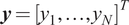
Table 2 presents the RMSE for all surfaces. Evidently, the BO-driven scanning method provides improved accuracy compared to the full scans produced by the conventional scanning method, while requiring significantly fewer measurements. Figure 12 provides a visualization of these RMSE values. Note that the RMSE for the conventional scanning method in this figure corresponds to the full scan. For all surface types, the predicted Bayesian surfaces are more accurate surface representations than the conventional scanning method.
Summary of the RMSE between the true surfaces and the point clouds found by using the BO-driven and conventional scanning methods for all surfaces
Comparison of the RMSE for: (a) flat surface, (b) hole surface, and (c) wave surface.

For the flat surface, the prediction RMSE increases with the number of measurements. For measurement counts below 80, BO scanning achieves lower RMSE than the conventional scanning method on the flat surface. In contrast, for the hole and wave surfaces, the prediction RMSE decreases as the number of measurements increases. For the hole surface, BO scanning outperforms the conventional method once the number of measurements exceeds approximately 50. For the wave surface, BO scanning performs particularly well, requiring only ∼20 measurements to surpass the conventional scanning method.
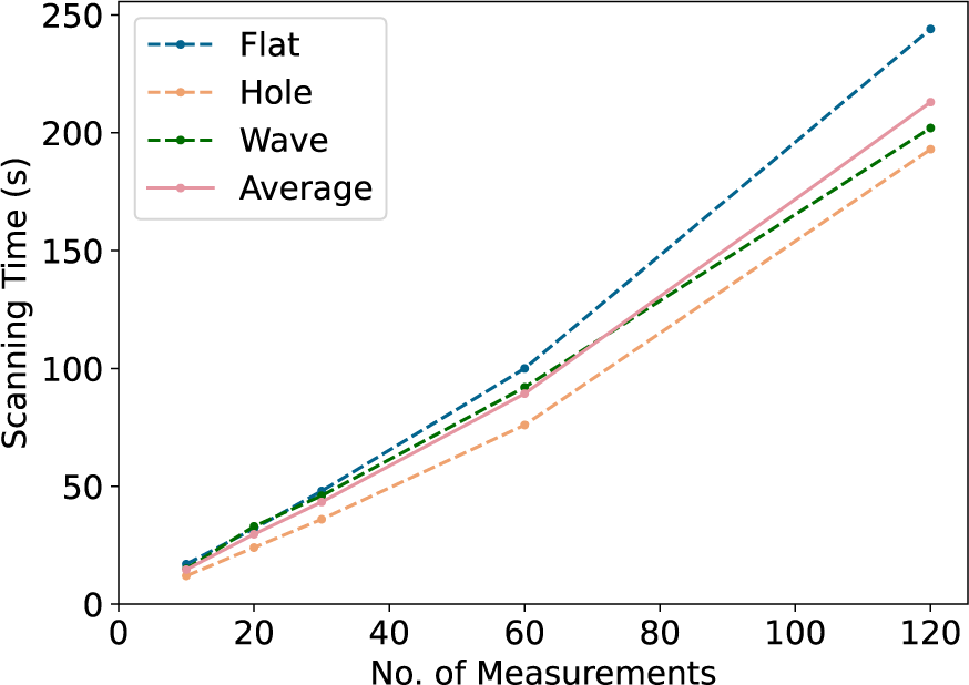
Figure 13 reports the measurement acquisition time, during Bayesian scanning, for each surface and the mean across surfaces. The average time per measurement is approximately 1.5 s for the first 60 measurements, increasing modestly to around 2.0 s for the final 60 measurements. This increase is consistent with longer BO computation times as the dataset grows and the next measurement location is selected in real time. Acquisition times are otherwise similar across the three surfaces, with the hole surface exhibiting a slightly lower average acquisition time than the flat and wave surfaces.
Comparison of the number of measurements vs the scanning time using the BO scanning method for all three surface types (flat, hole, and wave) and the average between them.

4. Discussion
The laboratory experiments demonstrate that the BO-driven scanning method with GP regression outperforms the conventional scanning method in most cases. One reason for the superior performance of the BO-driven method may be the ability of GP regression to handle noisy data. By incorporating noisy data into the Gaussian Process, the surface appears to be “smoothed out,” while the noise remains in the point clouds generated by the conventional method, leading to a higher RMSE. Additionally, the BO-driven method achieved this higher accuracy with fewer measurements than the conventional method.
For the flat surface, the BO-driven method outperformed the conventional method when fewer than 80 measurements were used. As more measurements were added, GP prediction RMSE increased, likely due to overfitting noisy observations and introducing spurious peaks and troughs. With fewer measurements, the GP tends to revert toward an approximately planar surface, which is more accurate here. For the hole surface, Figure 12b suggests that 50 measurements were required for the GP to match the conventional method. Figure 9a,b indicates the main errors occur near the hole edges, where measurements were limited and more variable. Near these edges, the echosounder may also pick up off-target returns (e.g., tank-wall echoes) when backscatter from the true surface is weak or highly oblique, which can mislead the GP. For the wave surface, Figure 12c suggests only 20 measurements were needed to achieve accuracy comparable to the conventional method. The geometry produces more favorable incidence angles toward the centre, improving echo detectability and reducing noise. In addition, the squared exponential kernel is well-suited to smooth, wave-like shapes, enabling accurate interpolation from sparse data.
On average, the BO-driven method required approximately 50 measurements to reconstruct 3D surfaces with higher accuracy than the conventional method. Using the acquisition-time relationship shown in Figure 13, this implies that, for a dual-axis scan spanning 360 x 30 degrees, the BO-driven approach would require, on average 1.5 minutes to produce an accurate scan, with the exact time depending on surface complexity. By contrast, a full conventional scan over the same angular range would require approximately 18 minutes and 2700 measurements. These results indicate that the BO-driven method improves accuracy while substantially reducing acquisition time. Further reductions in scanning time may be achievable with faster motors and upgraded computing hardware.
During the experiments, there were some anomalous results that were removed; these anomalies could arise from many different sources. Given the size of the water tank, there are likely two main causes. The first is that the echosounder is detecting reflections from the floor and walls of the tank as well as the support frame and mistaking those to be the test surface. The second is that an echosounder may struggle taking near-field measurements as the ultrasound beam requires a small distance to fully form and produce clear and easy to detect echoes when reflected. These two issues are exaggerated in the water tank and would be less present in a larger body of water. In addition, temperature fluctuations in the water; small floating rust flakes detached from nuts and bolts in the support frame; poor electrical connections from the echosounder to Raspberry Pi; and slight vibrations when the scanner moved could all effect measurements to some degree.
Using a sparser measurement pattern with the conventional scanning method could potentially reduce scanning times to match those of the BO-driven scanning method. However, the BO-driven method offers a key advantage: it adapts to the surface and selects sequentially optimal measurement locations, enabling accurate surface predictions in the shortest possible time. This adaptability is evident in the varying measurement patterns illustrated in Figures 7, 9, and 11. Unlike a conventional sparse scan, the BO-driven method is far less likely to miss critical areas of the surface. It begins by taking measurements distributed across the entire surface and, as the algorithm gains confidence in the surface’s shape, it concentrates on critical regions. This targeted approach significantly reduces the risk of overlooking important features. The selection of sequentially optimal measurement locations is especially important for scanning surfaces that change rapidly over time, which is a challenge not addressed in this paper. This limitation highlights an area for further exploration, and a future study has been planned to evaluate the performance of the BO-driven scanning method on dynamically changing surfaces.
The conventional scanning method typically produces large point cloud files, which can be challenging and time-consuming to process and analyze. In contrast, the BO-driven method requires fewer measurements to generate an accurate surface, significantly reducing the amount of data that needs to be stored. This decrease in data volume minimizes logging and transfer demands, making the method particularly advantageous for offshore applications, where slow data transmission speeds can be a constraint. Additionally, if the scanner were made wireless using ultrasonic modems, the smaller data size would be beneficial, given the limited bandwidth of these modems.
Despite the potential advantages of GP regression and BO data acquisition for underwater 3D scanning, several limitations should be noted. First, GP performance depends strongly on the choice of kernel, which encodes prior assumptions about surface structure. An inappropriate kernel can bias predictions and reduce accuracy. In addition, stationary kernels impose the same smoothness assumptions across the entire domain, which can be restrictive for highly irregular surfaces with spatially varying patterns. To support a general-purpose workflow, this study used the squared exponential kernel, which primarily assumes smooth, continuous variation. This kernel choice has been shown to perform reasonably well across a range of geometries associated with seabed deformation. Second, GP regression typically performs poorly for extrapolation. Because the model relies on local correlation (nearby measurements are expected to be similar), predictive performance degrades as the distance from observations increases, which can contribute to edge distortions in reconstructed surfaces. Finally, GP regression and BO can be computationally expensive. While this cost is modest for small scan areas, it can become a bottleneck as the domain grows and additional measurements are required, particularly when optimization and inference are performed in real time. This effect was observed in the experiments, where the acquisition of the final 60 measurements took slightly longer. Future work will evaluate strategies to reduce computational load, including a sliding-window approach (using only the most recent n measurements for optimization) and parallelization via multiple scanners operating concurrently.
5. Conclusion
An AI-driven method for underwater 3D point scanning using Bayesian Optimization and Gaussian Process regression was proposed and tested under laboratory conditions. The results show that the proposed method achieves accuracy comparable to, and in most cases better than, the conventional scanning approach. For example, for the wave surface, the proposed method reduced RMSE by approximately one-third relative to the conventional method. A key advantage is efficiency: accurate 3D surface reconstructions can be obtained in around 1.5 minutes using, on average, 50 measurements, whereas the conventional method requires approximately 18 minutes and 2700 measurements over the same scan range. Additionally, the proposed approach produces significantly smaller file sizes, simplifying data management and making it particularly suitable for scenarios with limited data transmission capabilities, such as deep-water applications involving wireless ultrasonic modems. However, the method has several limitations: it may perform less reliably on surfaces that are more complex or irregular than those examined here, and scanning larger areas may introduce edge artefacts and increase total acquisition time. Overall, this AI-driven scanning method offers a compelling alternative to traditional underwater 3D scanning techniques, combining improved speed, adaptability, and practicality with reduced data handling requirements.
Data availability statement
Measurements taken with the Bayesian and Conventional scanning methods, in terms of spherical polar coordinates for the flat, hole and wave surfaces, are available from: Benjamin-Strath (2026). Benjamin-Strath/AI-scanner-laboratory-experiment-data---Final: v1.0 (Data). Zenodo. https://doi.org/10.5281/zenodo.19629750
Author contribution
Conceptualization-Equal: B.W., S.S.; Data Curation-Equal: B.W.; Funding Acquisition-Equal: S.S.; Methodology-Equal: B.W., S.S., K.D., J.M.; Supervision-Equal: S.S.; Visualization-Equal: B.W., S.S.; Writing – Original Draft-Equal: B.W.; Writing – Review & Editing-Equal: B.W., S.S., K.D., J.M.
Funding statement
This research was supported by scholarships from the EPSRC DTP for sponsoring the doctoral studies of the first author. The second author would also like to thank the support of Royal Society for providing grants (RGS\R1\231,021) to support this research.
Competing interests
The authors declare none.
Ethical standard
The research meets all ethical guidelines, including adherence to the legal requirements of the study country.


 Open access
Comments
No Comments have been published for this article.