

1. Introduction
Shock models are adequate to describe the failure mechanism of systems, living organisms, or general items that are subject to stress or shocks during their working period. In this context, a device is initially active and it receives random shocks according to a counting process. In addition, the number of shocks that cause the failure of the device is itself random. Many contributions regarding shock models have been developed in different areas of the literature. We refer the reader to [Reference Cha and Finkelstein7, Reference Fagiuoli and Pellerey22, Reference Finkelstein and Cha24, Reference Pellerey32]. Moreover, aiming to deal with more general settings, multivariate shock models have been studied in various fields as well (see [Reference Belzunce, Lillo, Pellerey and Shaked5, Reference Cha and Badía6, Reference Eryilmaz21, Reference Mohtashami-Borzadaran, Jabbari and Amini29, Reference Pellerey33, Reference Shaked34, Reference Wong37]).
Often shock models follow the Poisson process as the underlying counting process, since it represents a good compromise between a realistic representation of the phenomena and mathematical tractability of the model (see, for instance, [Reference Di Crescenzo12, Reference Eryilmaz19, Reference Fagiuoli and Pellerey23]). However, in many practical situations, specific random occurrences of events in time cannot be adequately described by the Poisson process, since the assumption of independence between its increments is not feasible. Therefore, alternative counting processes to the Poisson one have been considered in view of managing shock models (see [Reference Cha and Finkelstein9, Reference Cha and Giorgio10, Reference Eryilmaz20, Reference Iuliano, Martinucci and Mustaro25]).
The geometric counting process deals with random occurrences between events that are not independent, and it represents another suitable alternative to the Poisson process (see [Reference Cha and Finkelstein8, Reference Di Crescenzo and Pellerey17]).
In this article, we study bivariate shock models in which shocks are governed by two homogeneous geometric counting processes, with possibly different intensities. Specifically, we consider the bivariate geometric counting process, which is a two-dimensional mixed Poisson process with mixing distribution given by the maximum of two exponential distributions. We face the problem when the intensities of baseline Poisson processes are shared, leading to the dependence between the marginal geometric counting processes.
The competing risks framework is also considered, by taking into account that failures are due to a single cause (risk). This model is of considerable interest in various fields (see [Reference Bedford and Cooke4, Reference Crowder11] as classical references). In reliability theory and survival analysis, Balakrishnan and Castilla [Reference Balakrishnan and Castilla3] developed robust inference for one-shot device test data with Weibull lifetimes under the competing risks scenario. Di Crescenzo and Longobardi [Reference Di Crescenzo and Longobardi13] proposed a version of the well-known ‘new better than used’ and ‘new worse than used’ ageing properties for random lifetimes within a specific cause of failure. Moreover, Di Crescenzo and Meoli [Reference Di Crescenzo and Meoli15] studied relations with copula and time-transformed exponential models. Competing risks are a common issue also in medical research. For instance, in cancer studies, both treatment-related death and disease recurrence are important outcomes. A classic example comes from studies on tumor-causing agents. Altshuler [Reference Altshuler2] proposed a method using Poisson processes to model these competing events, estimating biological activity over time. Kim [Reference Kim27] introduced statistical methods to analyze competing risks, by providing comparisons with their respective counterparts in standard survival analysis.
Since competing risks are noteworthy for the description of the failure of a complex system subject to different types of risk, we refer to observable pairs $(T,\delta)$
, where T is a nonnegative random variable, namely, random lifetime, that describes the time of failure of an item, while
$(T,\delta)$
, where T is a nonnegative random variable, namely, random lifetime, that describes the time of failure of an item, while $\delta$
describes the (exclusive) cause or type of failure. Di Crescenzo and Longobardi [Reference Di Crescenzo and Longobardi14] considered a formulation of the competing risks model within the framework of stochastic shock models governed by a bivariate Poisson process. Recently, Di Crescenzo and Meoli [Reference Di Crescenzo and Meoli16] and Soni et al. [Reference Soni, Pathak, Di Crescenzo and Meoli36] investigated different generalized versions of bivariate Poisson processes.
$\delta$
describes the (exclusive) cause or type of failure. Di Crescenzo and Longobardi [Reference Di Crescenzo and Longobardi14] considered a formulation of the competing risks model within the framework of stochastic shock models governed by a bivariate Poisson process. Recently, Di Crescenzo and Meoli [Reference Di Crescenzo and Meoli16] and Soni et al. [Reference Soni, Pathak, Di Crescenzo and Meoli36] investigated different generalized versions of bivariate Poisson processes.
The article is organized as follows. Section 2 is devoted to the description of the two-dimensional shock model within the competing risks framework, by our taking into account that failures are due to a single cause. The study is carried out in a general configuration, i.e. underlying counting processes and the failure pattern are not fixed. We also provide sufficient conditions for the independence between the random failure time T and the cause of failure $\delta$
. In Section 3 we assume that the shocks are driven by two homogeneous geometric counting processes
$\delta$
. In Section 3 we assume that the shocks are driven by two homogeneous geometric counting processes $N_1(t)$
and
$N_1(t)$
and $N_2(t)$
by providing the explicit expression of some relevant functions. In Section 4 failures are assumed to occur at the first instant in which
$N_2(t)$
by providing the explicit expression of some relevant functions. In Section 4 failures are assumed to occur at the first instant in which $N_1(t) + N_2(t) = M$
, where M is a random counting number, independent of
$N_1(t) + N_2(t) = M$
, where M is a random counting number, independent of $(N_1(t),N_2(t))$
. Special choices of the random threshold are considered too. Some final remarks are then given in Section 5.
$(N_1(t),N_2(t))$
. Special choices of the random threshold are considered too. Some final remarks are then given in Section 5.
Throughout this article the terms increasing and decreasing are used as meaning ‘nondecreasing’ and ‘nonincreasing’, respectively. Moreover, $\mathbb{R}^+$
denotes the set of positive real numbers,
$\mathbb{R}^+$
denotes the set of positive real numbers, $\mathbb{R}^+_0=\mathbb{R}^+\cup\{0\}$
,
$\mathbb{R}^+_0=\mathbb{R}^+\cup\{0\}$
, $\mathbb{N}$
denotes the set of positive integers, and
$\mathbb{N}$
denotes the set of positive integers, and $\mathbb{N}_0=\mathbb{N}\cup\{0\}$
.
$\mathbb{N}_0=\mathbb{N}\cup\{0\}$
.
2. Bivariate Shock Models within Competing Risks
In this section we describe and study the bivariate shock model driven by (generic) counting processes within the competing risks framework. In particular, we provide sufficient conditions for which the failure time and the cause of failure are independent.
Let T be a random lifetime with an absolutely continuous distribution that describes the failure time of an item (system or a living organism) having survival function (SF) defined as $\overline{F}_T(t)=\mathbb{P}(T>t)$
for
$\overline{F}_T(t)=\mathbb{P}(T>t)$
for $t\ge 0$
. We assume that the item is initially active, i.e.
$t\ge 0$
. We assume that the item is initially active, i.e. $\overline{F}_T(0)=1$
. Moreover, it fails in a certain instant, so that
$\overline{F}_T(0)=1$
. Moreover, it fails in a certain instant, so that $\lim_{t\to +\infty}\overline{F}_T(t)=0$
. Let
$\lim_{t\to +\infty}\overline{F}_T(t)=0$
. Let $\delta=i$
if the failure occurs due to a shock of type i for
$\delta=i$
if the failure occurs due to a shock of type i for $i=1,2$
. We denote by
$i=1,2$
. We denote by $N_i(t)$
, for
$N_i(t)$
, for $i=1,2$
, the counting process representing the number of shocks of type i occurring in [0, t].
$i=1,2$
, the counting process representing the number of shocks of type i occurring in [0, t].
We can partition the state space $\mathbb{N}^2_0$
of
$\mathbb{N}^2_0$
of $(N_1(t),N_2(t))$
into nonempty subsets
$(N_1(t),N_2(t))$
into nonempty subsets
 \begin{equation}S_k\;:\!=\;\{(x_1,x_2)\in \mathbb{N}^2_0\;:\;\Psi (x_1,x_2)=k\}, \qquad k\in\mathbb{N}_0,\end{equation}
called failure sets, where $\Psi\;:\;\mathbb{N}^2_0\longrightarrow\mathbb{N}$
is a given suitable function that creates a partition of the state space. We assume that
$\Psi\;:\;\mathbb{N}^2_0\longrightarrow\mathbb{N}$
is a given suitable function that creates a partition of the state space. We assume that $S_0$
includes the numbers of nonfatal shocks; namely, if
$S_0$
includes the numbers of nonfatal shocks; namely, if $(N_1(t),N_2(t))\in S_0$
then the shocks that arrived up to time t do not cause a failure.
$(N_1(t),N_2(t))\in S_0$
then the shocks that arrived up to time t do not cause a failure.
We denote by M the integer-valued random variable that represents the index of which failure set $S_k$
,
$S_k$
, $k\in\mathbb{N}$
, contains the numbers of fatal shocks, independent of
$k\in\mathbb{N}$
, contains the numbers of fatal shocks, independent of $(N_1(t),N_2(t))$
. In other words,
$(N_1(t),N_2(t))$
. In other words, $M=k$
if and only if the system fails at the first instant
$M=k$
if and only if the system fails at the first instant $t>0$
in which
$t>0$
in which $(N_1(t),N_2(t))\in S_k$
. For
$(N_1(t),N_2(t))\in S_k$
. For $k\in\mathbb{N}$
the risky sets are defined as
$k\in\mathbb{N}$
the risky sets are defined as
 \begin{equation}\begin{array}{l}R_k^{(1)}\;:\!=\; \{(x_1,x_2)\in \mathbb{N}^2_0\setminus S_k\;:\;(x_1+1,x_2)\in S_k\}, \\[5pt] R_k^{(2)}\;:\!=\;\{(x_1,x_2)\in \mathbb{N}^2_0\setminus S_k\;:\;(x_1,x_2+1)\in S_k\},\end{array}\end{equation}
where $R_k^{(i)}$
,
$R_k^{(i)}$
, $i=1,2$
, contains all states of
$i=1,2$
, contains all states of $\mathbb{N}^2_0$
leading to a failure at time t at the next occurrence of a shock of type i, given that
$\mathbb{N}^2_0$
leading to a failure at time t at the next occurrence of a shock of type i, given that $M=k$
. Note that, from (2), the failures are due to a single cause. In addition, we remark that in general
$M=k$
. Note that, from (2), the failures are due to a single cause. In addition, we remark that in general $R_k^{(i)}$
is different from
$R_k^{(i)}$
is different from $S_{k-1}$
. Under these assumptions, the failure time can be denoted as
$S_{k-1}$
. Under these assumptions, the failure time can be denoted as
 $$T=\inf\{t\ge 0 \;:\; \Psi\left(N_1(t),N_2(t)\right)=M\}.$$
The probability density function (PDF) of T is expressed as
 $$f_T(t)=f_1(t)+f_2(t),\qquad t\geq 0,$$
where $f_i$
, for
$f_i$
, for $i=1,2$
, is the failure density (FD), also named subdensity function, defined by
$i=1,2$
, is the failure density (FD), also named subdensity function, defined by
 \begin{equation}f_i(t)=\frac{\textrm{d}}{\textrm{d}t}\mathbb{P}\{T\leq t,\,\delta=i\}, \qquad t\geq 0.\end{equation}
Note that $f_i$
, for
$f_i$
, for $i=1,2$
, is not a proper PDF. Indeed, since
$i=1,2$
, is not a proper PDF. Indeed, since $\delta=i$
, when the failure occurs due to a shock of type i, we have
$\delta=i$
, when the failure occurs due to a shock of type i, we have
 \begin{equation}\mathbb{P}(\delta=i)=\int_0^{+\infty} f_i(t)\,\textrm{d}t,\qquad i=1,2.\end{equation}
From (3) and (4), we can obtain the moments of the failure time conditioned on the cause of failure for $s\ge 1$
as
$s\ge 1$
as
 \begin{equation}\mathbb{E}(T^s\,|\,\delta=i)=\frac{1}{\mathbb{P}(\delta=i)}\int_{0}^{+\infty} t^s\,f_i(t)\,\textrm{d}t, \qquad i=1,2.\end{equation}
To express the FDs $f_i$
for
$f_i$
for $i=1,2$
in terms of the joint probability distribution of
$i=1,2$
in terms of the joint probability distribution of $(N_1(t),N_2(t))$
, we introduce the following hazard rates:
$(N_1(t),N_2(t))$
, we introduce the following hazard rates:
 \begin{equation}\begin{array}{l}r_1(x_1,x_2;\; t)=\displaystyle\lim_{\tau\to 0^+} \frac{1}{\tau}\mathbb{P}[N_1(t+\tau)= x_1+1, N_2(t+\tau)= x_2| N_1(t)=x_1, N_2(t)=x_2], \\[9pt] r_2(x_1,x_2;\; t)=\displaystyle\lim_{\tau\to 0^+} \frac{1}{\tau}\mathbb{P}[N_1(t+\tau)= x_1, N_2(t+\tau)= x_2+1| N_1(t)=x_1, N_2(t)=x_2],\end{array}\end{equation}
with $(x_1,x_2)\in\mathbb{N}^2_0$
and
$(x_1,x_2)\in\mathbb{N}^2_0$
and $t\geq 0$
. Hence, given that
$t\geq 0$
. Hence, given that $x_1$
shocks of type 1 and
$x_1$
shocks of type 1 and $x_2$
shocks of type 2 occurred in [0, t],
$x_2$
shocks of type 2 occurred in [0, t], $r_i(x_1,x_2;\; t)$
gives the intensity of the occurrence of a shock of type i immediately after t, with
$r_i(x_1,x_2;\; t)$
gives the intensity of the occurrence of a shock of type i immediately after t, with $i=1,2$
. Note that
$i=1,2$
. Note that $r_1(x_1,x_2;\; t)+r_2(x_1,x_2;\; t)$
is the hazard rate of a shock of any type.
$r_1(x_1,x_2;\; t)+r_2(x_1,x_2;\; t)$
is the hazard rate of a shock of any type.
From the assumptions stated above, the item fails at time t due to a shock of type i if the two-dimensional counting process $(N_1(t),N_2(t))$
takes values in
$(N_1(t),N_2(t))$
takes values in $R_k^{(i)}$
at time t and a shock of type i occurs immediately after. Hence, conditioning on M and recalling (2) and (6), for
$R_k^{(i)}$
at time t and a shock of type i occurs immediately after. Hence, conditioning on M and recalling (2) and (6), for $i=1,2$
, we have
$i=1,2$
, we have
 \begin{equation}f_i(t)=\sum_{k=1}^{+\infty} p_M(k) \sum_{(x_1,x_2)\in R_k^{(i)}}\mathbb{P}[N_1(t)=x_1,N_2(t)=x_2]\,r_i(x_1,x_2;\;t),\qquad t\ge 0,\end{equation}
where $p_M(k)=\mathbb{P}(M=k)$
, for
$p_M(k)=\mathbb{P}(M=k)$
, for $k\in\mathbb{N}$
, denotes the probability distribution of M. Therefore, by using (7), we can express (4) and (5) in terms of the joint probability distribution of
$k\in\mathbb{N}$
, denotes the probability distribution of M. Therefore, by using (7), we can express (4) and (5) in terms of the joint probability distribution of $(N_1(t),N_2(t))$
.
$(N_1(t),N_2(t))$
.
We recall that a multivariate counting process $\{\textbf{N}(t), t\in\mathbb{R}^+_0\}$
has the multinomial property if the identity
$\{\textbf{N}(t), t\in\mathbb{R}^+_0\}$
has the multinomial property if the identity
 \begin{equation}\begin{aligned}&\mathbb{P}\left[\bigcap_{j=1}^m \left\{\textbf{N}(t_j) -\textbf{N}(t_{j-1})=\textbf{n}_j \right\}\right]\\[5pt] &=\left(\prod_{i=1}^\ell\frac{\left( \sum_{j=1}^m n_j^{(i)} \right)!}{\prod_{j=1}^m n_j^{(i)}!}\prod_{j=1}^m\left(\frac{t_j - t_{j-1}}{t_m}\right)^{n_j^{(i)}}\right)\mathbb{P}\left[\left\{\textbf{N}(t_m)=\sum_{j=1}^m \textbf{n}_j\right\}\right] \end{aligned}\end{equation}
holds for all $m \in \mathbb{N}$
and
$m \in \mathbb{N}$
and $t_0, t_1, \ldots, t_m\in\mathbb{R}^+_0$
with
$t_0, t_1, \ldots, t_m\in\mathbb{R}^+_0$
with $0 = t_0 < t_1 < \cdots < t_m$
, and for all
$0 = t_0 < t_1 < \cdots < t_m$
, and for all $\textbf{n}_j \in \mathbb{N}_0^\ell$
,
$\textbf{n}_j \in \mathbb{N}_0^\ell$
, $j \in \{1, \ldots, m\}$
; see Section 2.2 in [Reference Zocher38]. Hereafter, we characterize the expression for the FDs given in (7) by assuming that the corresponding bivariate counting process has the multinomial property.
$j \in \{1, \ldots, m\}$
; see Section 2.2 in [Reference Zocher38]. Hereafter, we characterize the expression for the FDs given in (7) by assuming that the corresponding bivariate counting process has the multinomial property.
Proposition 1. If $\textbf{N}(t)=(N_1(t),N_2(t))$
has the multinomial property, then
$\textbf{N}(t)=(N_1(t),N_2(t))$
has the multinomial property, then
 \begin{equation}f_i(t)=\sum_{k=1}^{+\infty}p_M(k)\sum_{(x_1,x_2)\in R^{(i)}_k}(x_i+1)t^{x_1+x_2}\lim_{\tau\to 0^+}\frac{\mathbb{P}[N_i(t+\tau)=x_i+1,N_j(t+\tau)=x_j]}{(t+\tau)^{x_1+x_2+1}}\end{equation}
for $i=1,2$
,
$i=1,2$
, $j=3-i$
, and
$j=3-i$
, and $t\ge 0$
.
$t\ge 0$
.
Proof. We prove the result for $i=1$
, since in a similar way it follows for
$i=1$
, since in a similar way it follows for $i=2$
. From (6), we have
$i=2$
. From (6), we have
 $$\displaystyle\begin{aligned}&r_1(x_1,x_2;\;t)\\[5pt] &=\lim_{\tau\to 0^+}\frac{1}{\tau}\frac{\mathbb{P}\left[N_1(t+\tau)=x_1+1, N_2(t+\tau)=x_2, N_1(t)=x_1, N_2(t)=x_2\right]}{\mathbb{P}\left[\left(N_1(t),N_2(t)\right)=(x_1,x_2)\right]}\\[5pt] &=\lim_{\tau\to 0^+}\frac{1}{\tau}\frac{\mathbb{P}\left[\{\left(N_1(t),N_2(t)\right)=(x_1,x_2)\}\cap\{\left(N_1(t+\tau)-N_1(t),N_2(t+\tau)-N_2(t)\right)=(1,0)\}\right]}{\mathbb{P}\left[\left(N_1(t),N_2(t)\right)=(x_1,x_2)\right]}\\[5pt] &=(x_1+1)t^{x_1+x_2}\lim_{\tau\to 0^+}\frac{\mathbb{P}\left[\left(N_1(t+\tau),N_2(t+\tau)\right)=(x_1+1,x_2)\right]}{(t+\tau)^{x_1+x_2+1}\,\mathbb{P}\left[\left(N_1(t),N_2(t)\right)=(x_1,x_2)\right]},\end{aligned}$$
having used in the last equality the multinomial property given in (8) for $\ell=m=2$
. Hence, the result follows by applying the latter expression in (7).
$\ell=m=2$
. Hence, the result follows by applying the latter expression in (7).
Since $\{T>t\}=\{\Psi\left(N_1(t),N_2(t)\right)<M\}$
for all
$\{T>t\}=\{\Psi\left(N_1(t),N_2(t)\right)<M\}$
for all $t\ge 0$
, by conditioning on
$t\ge 0$
, by conditioning on $(N_1(t),N_2(t))$
, from (1) we obtain
$(N_1(t),N_2(t))$
, from (1) we obtain
 \begin{equation}\overline F_T(t)=\sum_{k=0}^{+\infty} \overline F_M(k) \sum_{(x_1,x_2)\in S_k}\mathbb{P}[N_1(t)=x_1,N_2(t)=x_2], \qquad t\geq 0,\end{equation}
where $\overline F_M(k)$
, for
$\overline F_M(k)$
, for $k\in\mathbb{N}_0$
, is the SF of M such that
$k\in\mathbb{N}_0$
, is the SF of M such that $\overline F_M(0)=1$
.
$\overline F_M(0)=1$
.
Remark 1. Let us assume that two random thresholds $M_1$
and
$M_1$
and $M_2$
are ordered in the usual stochastic sense; that is,
$M_2$
are ordered in the usual stochastic sense; that is, $\overline{F}_{M_1}(k)\le\overline{F}_{M_2}(k)$
for all
$\overline{F}_{M_1}(k)\le\overline{F}_{M_2}(k)$
for all $k\in\mathbb{N}_0$
(denoted as
$k\in\mathbb{N}_0$
(denoted as $M_1\le_{\mathrm{st}}M_2$
). Therefore, from (10), if the corresponding random failure times
$M_1\le_{\mathrm{st}}M_2$
). Therefore, from (10), if the corresponding random failure times $T_1$
and
$T_1$
and $T_2$
are conditioned on the same pair of counting processes, according to the same failure scheme, then
$T_2$
are conditioned on the same pair of counting processes, according to the same failure scheme, then $T_1\le_{\mathrm{st}}T_2$
. For more details about stochastic orders, we refer the reader to [Reference Shaked and Shanthikumar35]. Moreover, see [Reference Pellerey31] for stochastic comparisons between random lifetimes in the context of shock models driven by univariate counting processes.
$T_1\le_{\mathrm{st}}T_2$
. For more details about stochastic orders, we refer the reader to [Reference Shaked and Shanthikumar35]. Moreover, see [Reference Pellerey31] for stochastic comparisons between random lifetimes in the context of shock models driven by univariate counting processes.
Hereafter we provide sufficient conditions for which the random failure time T and the cause of failure $\delta$
are independent. We refer to [Reference Kella26] for a characterization of the independence between time and cause of failure for a general item.
$\delta$
are independent. We refer to [Reference Kella26] for a characterization of the independence between time and cause of failure for a general item.
Theorem 1. In (1), let us assume $\Psi(x_1, x_2)=\Psi(x_2, x_1)$
for all
$\Psi(x_1, x_2)=\Psi(x_2, x_1)$
for all $(x_1,x_2)\in \mathbb{N}^2_0$
. If
$(x_1,x_2)\in \mathbb{N}^2_0$
. If
 \begin{equation}(N_1(t),N_2(t))=_{\mathrm{st}}(N_2(t),N_1(t))\quad \mbox{for all} \ t\ge 0,\end{equation}
then T and $\delta$
are independent, where
$\delta$
are independent, where $=_{\mathrm{st}}$
means equality in law.
$=_{\mathrm{st}}$
means equality in law.
Proof. Under the stated hypothesis on $\Psi$
, from (2) it is easy to see that
$\Psi$
, from (2) it is easy to see that $(x_1,x_2)\in R_k^{(1)}$
if and only if
$(x_1,x_2)\in R_k^{(1)}$
if and only if $(x_2,x_1)\in R_k^{(2)}$
, for any
$(x_2,x_1)\in R_k^{(2)}$
, for any $(x_1,x_2)\in \mathbb{N}^2_0$
. Therefore, from (7), by using (11), it follows that
$(x_1,x_2)\in \mathbb{N}^2_0$
. Therefore, from (7), by using (11), it follows that $f_1(t)=f_2(t)$
for all
$f_1(t)=f_2(t)$
for all $t\ge 0$
. Hence, from (4) we have
$t\ge 0$
. Hence, from (4) we have $\mathbb{P}(\delta=1)=\mathbb{P}(\delta=2)=1/2$
, which allows us to obtain for
$\mathbb{P}(\delta=1)=\mathbb{P}(\delta=2)=1/2$
, which allows us to obtain for $i=1,2$
 $$\mathbb{P}(\delta=i)f_T(t)=f_i(t),\qquad t\ge 0,$$
and the proof is completed.
From this point on we assume that shocks are driven by homogeneous geometric counting processes.
3. Results under the Geometric Counting Process
In this section we assume that the two kinds of shock affect the system according to homogeneous geometric counting processes $N_1(t)$
and
$N_1(t)$
and $N_2(t)$
, respectively. The definition of the geometric counting process can be stated as follows.
$N_2(t)$
, respectively. The definition of the geometric counting process can be stated as follows.
Definition 1. Let $\{N^{(\alpha)}(t), t\in\mathbb{R}^+_0\}$
be a Poisson process with intensity
$\{N^{(\alpha)}(t), t\in\mathbb{R}^+_0\}$
be a Poisson process with intensity $\alpha$
. Let U be an exponential distribution with mean
$\alpha$
. Let U be an exponential distribution with mean $\lambda\in\mathbb{R}^+$
. The process
$\lambda\in\mathbb{R}^+$
. The process $\{N(t),t\in\mathbb{R}^+_0\}$
having marginal distributions for
$\{N(t),t\in\mathbb{R}^+_0\}$
having marginal distributions for $x\in\mathbb{N}_0$
given by
$x\in\mathbb{N}_0$
given by
 $$\mathbb{P}\left[N(t)=x\right]=\int_{0}^{+\infty}\mathbb{P}\big[N^{(\alpha)}(t)=x\big]\textrm{d}U(\alpha),\qquad t\in\mathbb{R}^+_0,$$
is named geometric counting process with intensity $\lambda$
.
$\lambda$
.
We now extend the geometric counting process to the bivariate case.
Definition 2. Let $\{N_1^{(\alpha)}(t), t\in\mathbb{R}^+_0\}$
and
$\{N_1^{(\alpha)}(t), t\in\mathbb{R}^+_0\}$
and $\{N_2^{(\alpha)}(t), t\in\mathbb{R}^+_0\}$
be independent Poisson processes, both having intensity
$\{N_2^{(\alpha)}(t), t\in\mathbb{R}^+_0\}$
be independent Poisson processes, both having intensity $\alpha\in\mathbb{R}^+$
. Let U be the distribution of
$\alpha\in\mathbb{R}^+$
. Let U be the distribution of $\max\{T_1,T_2\}$
, where
$\max\{T_1,T_2\}$
, where $T_i$
has an exponential distribution with mean
$T_i$
has an exponential distribution with mean $\frac1{\lambda_i}\in\mathbb{R}^+$
for
$\frac1{\lambda_i}\in\mathbb{R}^+$
for $i=1,2$
. The bivariate process
$i=1,2$
. The bivariate process $\boldsymbol{N}(t)=(N_1(t),N_2(t))$
, for
$\boldsymbol{N}(t)=(N_1(t),N_2(t))$
, for $t\in\mathbb{R}^+_0$
, having joint distribution for
$t\in\mathbb{R}^+_0$
, having joint distribution for $x_1,x_2\in \mathbb{N}_0$
given by
$x_1,x_2\in \mathbb{N}_0$
given by
 \begin{equation}\mathbb{P}[N_1(t)=x_1,N_2(t)=x_2]=\int_{\mathbb{R}^+}\mathbb{P}\big[N_1^{(\alpha)}(t)=x_1,N_2^{(\alpha)}(t)=x_2\big]\textrm{d}U(\alpha),\qquad t\in\mathbb{R}^+_0,\end{equation}
is named bivariate geometric counting process, where the intensity of $N_i$
is 1/
$N_i$
is 1/ $\lambda_i$
, for
$\lambda_i$
, for $i=1,2$
.
$i=1,2$
.
Remark 2. By taking into account Lemma 3.1.1 in [Reference Zocher38], the bivariate geometric counting process in (12) has the multinomial property given in (8). Then it satisfies the assumptions of Proposition 1.
For the next result we recall that the gamma function is defined as
 \begin{equation}\Gamma(z)\;:\!=\;\int_0^{+\infty}t^{z-1}\mathrm{e}^{-t}\textrm{d}t,\end{equation}
with $Re(z)>0$
(see, for instance, the equation 6.1.1 in [Reference Abramowitz and Stegun1]).
$Re(z)>0$
(see, for instance, the equation 6.1.1 in [Reference Abramowitz and Stegun1]).
Proposition 2. Under the assumptions of Definition 2, if $T_1$
and
$T_1$
and $T_2$
are independent, then
$T_2$
are independent, then
 \begin{equation}\begin{aligned}&\mathbb{P}\left[N_1(t)=x_1,N_2(t)=x_2\right]=\left(\substack{x_1+x_2\\ x_1}\right)t^{x_1+x_2}\\[5pt] &\quad\times\left[\frac{\lambda_1}{(2t+\lambda_1)^{x_1+x_2+1}}+\frac{\lambda_2}{(2t+\lambda_2)^{x_1+x_2+1}}-\frac{\lambda_1+\lambda_2}{(2t+\lambda_1+\lambda_2)^{x_1+x_2+1}}\right] \end{aligned}\end{equation}
for $x_1,x_2\in \mathbb{N}_0$
.
$x_1,x_2\in \mathbb{N}_0$
.
Proof. Under the stated hypothesis, from (12) it holds that
 $$\begin{aligned}&\mathbb{P}\left[N_1(t)=x_1,N_2(t)=x_2\right]\\[5pt] &\quad =\int_{\mathbb{R}^+}\mathrm{e}^{-2\alpha t}\frac{(\alpha t)^{x_1+x_2}}{x_1!x_2!}\left[\lambda_1\mathrm{e}^{-\lambda_1\alpha}(1-e^{-\lambda_2\alpha})+\lambda_2\mathrm{e}^{-\lambda_2\alpha}(1-\mathrm{e}^{-\lambda_1\alpha})\right]\textrm{ d}\alpha\\[5pt] &\quad =\frac{t^{x_1+x_2}\left[h(x_1+x_2;\;\lambda_1)+h(x_1+x_2;\;\lambda_2)- h(x_1+x_2;\;\lambda_1+\lambda_2)\right]}{x_1!x_2!}, \end{aligned}$$
where
 $$h(x;\;\lambda)\;:\!=\;\int_0^{+\infty} \lambda\alpha^{x} \mathrm{e}^{-\alpha(2t+\lambda)}\textrm{d}\alpha=\frac{\lambda\Gamma(x+1)}{(2t+\lambda)^{x+1}},$$
having set $u=\alpha(2t+\lambda)$
in the last equality and by recalling (13). Then, since
$u=\alpha(2t+\lambda)$
in the last equality and by recalling (13). Then, since $\Gamma(x+1)=x!$
, for
$\Gamma(x+1)=x!$
, for $x\in\mathbb{N}_0$
, the thesis follows by straightforward calculations.
$x\in\mathbb{N}_0$
, the thesis follows by straightforward calculations.
Note that, under the assumptions of Proposition 2, (11) holds. Moreover, (14) can be rewritten as
 $$\mathbb{P}\left[N_1(t)=x_1,N_2(t)=x_2\right]=\left(\begin{array}{c}x_1+x_2 \\[2pt] x_1\end{array}\right)\frac{1}{2^{x_1+x_2}}\mathbb{P}\left[\tilde{N}^{(2\max\{T_1,T_2\})}(t)=x_1+x_2\right]\!,$$
where $T_1$
and
$T_1$
and $T_2$
are independent exponential random variables with means
$T_2$
are independent exponential random variables with means $1/\lambda_1$
and
$1/\lambda_1$
and $1/\lambda_2$
, respectively, and
$1/\lambda_2$
, respectively, and $\tilde{N}^{(\alpha)}(t)$
denotes a Poisson process with intensity
$\tilde{N}^{(\alpha)}(t)$
denotes a Poisson process with intensity $\alpha\in\mathbb{R}^+$
and that is independent of
$\alpha\in\mathbb{R}^+$
and that is independent of $T_1$
and
$T_1$
and $T_2$
.
$T_2$
.
As a consequence of Remark 2 and Proposition 2, from (9) it follows that
 \begin{equation}\begin{aligned}f_i(t)&=\sum_{k=1}^{+\infty}p_M(k)\sum_{(x_1,x_2)\in R^{(i)}_k}(x_1+x_2+1)\left(\begin{array}{c}x_1+x_2 \\[2pt] x_1\end{array}\right)t^{x_1+x_2}\\[5pt] &\quad\times \left[\frac{\lambda_1}{(2t+\lambda_1)^{x_1+x_2+2}}+\frac{\lambda_2}{(2t+\lambda_2)^{x_1+x_2+2}}-\frac{\lambda_1+\lambda_2}{(2t+\lambda_1+\lambda_2)^{x_1+x_2+2}}\right] \end{aligned}\end{equation}
for $i=1,2$
and
$i=1,2$
and $t\ge 0$
. Moreover, from (10) and (14), the SF of T becomes
$t\ge 0$
. Moreover, from (10) and (14), the SF of T becomes
 \begin{equation}\begin{aligned}\overline{F}_T(t)=&\sum_{k=0}^{+\infty}\overline{F}_M(k)\sum_{(x_1,x_2)\in S_k}\left(\begin{array}{c}x_1+x_2 \\[2pt] x_1\end{array}\right)t^{x_1+x_2}\\[5pt] &\times\left[\frac{\lambda_1}{(2t+\lambda_1)^{x_1+x_2+1}}+\frac{\lambda_2}{(2t+\lambda_2)^{x_1+x_2+1}}-\frac{\lambda_1+\lambda_2}{(2t+\lambda_1+\lambda_2)^{x_1+x_2+1}}\right] \end{aligned}\end{equation}
for $t\ge 0$
.
$t\ge 0$
.
We now specify the expression for the probability of the cause of failure given in (4) under the hypothesis that shocks are governed by the bivariate geometric counting process having probability law given in (14). For this aim, we recall that the well-known beta function can be expressed as
 \begin{equation}B(z,w)=\int_0^{+\infty}\frac{t^{z-1}}{(t+1)^{z+w}}\textrm{d}t,\end{equation}
which converges if $\mathrm{Re}(z)>0$
and
$\mathrm{Re}(z)>0$
and $\mathrm{Re}(w)>0$
(see, for instance, the equation 6.2.1 in [Reference Abramowitz and Stegun1]).
$\mathrm{Re}(w)>0$
(see, for instance, the equation 6.2.1 in [Reference Abramowitz and Stegun1]).
Proposition 3. Under the above assumptions, for $i=1,2$
it follows that
$i=1,2$
it follows that
 \begin{equation}\mathbb{P}(\delta=i)=\sum_{k=1}^{+\infty}p_M(k)\sum_{(x_1,x_2)\in R_k^{(i)}}\left(\begin{array}{c}x_1+x_2 \\[2pt] x_1\end{array}\right)2^{-x_1-x_2-1}.\end{equation}
Proof. Without loss of generality we prove the result for $i=1$
. From (4) and (15) we have
$i=1$
. From (4) and (15) we have
 $$\mathbb{P}(\delta=1)=\sum_{k=1}^{+\infty}p_M(k)\sum_{(x_1,x_2)\in R_k^{(1)}}(x_1+x_2+1)\left(\begin{array}{c}x_1+x_2 \\[2pt] x_1\end{array}\right)\varphi(x_1+x_2), $$
where
 $$\varphi(x)\;:\!=\;\int_0^{+\infty}\frac{\lambda t^{x}}{(2t+\lambda)^{x+2}}\textrm{d}t=2^{-x-1}B(x+1,1),$$
having set $y=2t/\lambda$
in the integral and by recalling (17). Then, since
$y=2t/\lambda$
in the integral and by recalling (17). Then, since $B(x,1)=1/x$
, (18) follows by straightforward calculations.
$B(x,1)=1/x$
, (18) follows by straightforward calculations.
Note that, from (18), the probability of the cause of failure does not depend on the respective intensities $\lambda_1$
and
$\lambda_1$
and $\lambda_2$
of the geometric counting processes.
$\lambda_2$
of the geometric counting processes.
Hereafter we prove that, in the proposed competing risks framework, the conditioned moments of the failure time T given in (5) diverge for all $s\ge 1$
.
$s\ge 1$
.
Proposition 4. Under the above assumptions, for $i=1,2$
it follows that
$i=1,2$
it follows that
 $$\mathbb{E}(T^s|\delta=i)=+\infty,\quad s\ge 1.$$
Proof. For $i=1$
, from (5) and (15) we have
$i=1$
, from (5) and (15) we have
 \begin{equation*}\begin{aligned}&\mathbb{P}(\delta=1)\mathbb{E}(T^s|\delta=1)\\[5pt] &\quad =\sum_{k=1}^{+\infty}p_M(k)\sum_{(x_1,x_2)\in R_k^{(1)}}(x_1+x_2+1)\left(\substack{x_1+x_2\\ x_1}\right)\\[5pt] &\qquad\times\left[g(x_1+x_2;\;s;\;\lambda_1)+g(x_1+x_2;\;s;\;\lambda_2)-g(x_1+x_2;\;s;\;\lambda_1+\lambda_2)\right]\\[5pt] &\quad =\sum_{k=1}^{+\infty}p_M(k)\sum_{(x_1,x_2)\in R_k^{(1)}}(x_1+x_2+1)\left(\substack{x_1+x_2\\ x_1}\right)\\[5pt] &\qquad\times\frac{[\lambda_1^s+\lambda_2^s-(\lambda_1+\lambda_2)^s]B(x_1+x_2+s+1,1-s)}{2^{x_1+x_2+s+1}}, \end{aligned}\end{equation*}
where
 $$g(x;\;s;\;\lambda)\;:\!=\;\int_0^{+\infty}\frac{\lambda t^{x+s}}{(2t+\lambda)^{x+2}}\textrm{d}t=\frac{\lambda^s B(x+s+1,1-s)}{2^{x+s+1}},$$
having set $y=2t/\lambda$
in the integral and by recalling (17). We can do the same similarly for
$y=2t/\lambda$
in the integral and by recalling (17). We can do the same similarly for $i=2$
. Hence, from (5), the thesis follows since
$i=2$
. Hence, from (5), the thesis follows since $B(x_1+x_2+s+1,1-s)=+\infty$
for all
$B(x_1+x_2+s+1,1-s)=+\infty$
for all $s\ge 1$
.
$s\ge 1$
.
Clearly, from the above results, the nature of the shock model is completely specified when the structures of the failure sets and of the risky sets are fixed. Hence, in the rest of this article, we consider a special case for the failure scheme. Specifically, by recalling (1), we assume that $\Psi(x_1,x_2)=x_1+x_2$
.
$\Psi(x_1,x_2)=x_1+x_2$
.
4. Failures due to the Sum of Shocks
In this section we assume that the system fails when the sum of shocks of type 1 and of type 2 reaches a random threshold that takes values in $\mathbb{N}$
, keeping in mind that shocks are driven by the bivariate geometric counting process having probability law given in (14). Hence, from (1) we have
$\mathbb{N}$
, keeping in mind that shocks are driven by the bivariate geometric counting process having probability law given in (14). Hence, from (1) we have
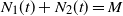
 \begin{equation}S_k= \{(x_1,x_2)\in \mathbb{N}^2_0\;:\; x_1+x_2=k\},\qquad k\in\mathbb{N}_0,\end{equation}
and
 \begin{equation}R_k^{(1)}=R_k^{(2)}=S_{k-1}, \qquad k\in\mathbb{N};\end{equation}
see Figure 1. Note that $S_0=\{(0,0)\}$
, which corresponds to no shocks of any kind having occurred during the system’s working period.
$S_0=\{(0,0)\}$
, which corresponds to no shocks of any kind having occurred during the system’s working period.
Failure scheme due to the sum of shocks.

Remark 3. From (14) and (19), the assumptions of Theorem 1 are satisfied, and thus T and $\delta$
are independent. It also holds that
$\delta$
are independent. It also holds that $f_1=f_2$
and
$f_1=f_2$
and $\mathbb{P}\left(\delta=1\right)=\mathbb{P}\left(\delta=2\right)=1/2$
.
$\mathbb{P}\left(\delta=1\right)=\mathbb{P}\left(\delta=2\right)=1/2$
.
In reliability theory, such a model may be appropriate to describe, for instance, the failure of systems made of units connected in series, as described below.
Remark 4. Let $X_1$
and
$X_1$
and $X_2$
describe the respective random failure time of two components in a series system having random lifetime denoted by
$X_2$
describe the respective random failure time of two components in a series system having random lifetime denoted by $T=\min\{X_1,X_2\}$
. We assume that the component with lifetime
$T=\min\{X_1,X_2\}$
. We assume that the component with lifetime $X_i$
is subject to a shock of type i for
$X_i$
is subject to a shock of type i for $i=1,2$
. If
$i=1,2$
. If $\delta$
denotes the related cause of failure, then
$\delta$
denotes the related cause of failure, then
 $$\mathbb{P}\left(\delta=i\right)=\mathbb{P}\left(X_i=T\right),\qquad i=1,2.$$
An example of this kind of system is given in Figure 2. For more details about system reliability theory, we refer the reader to [Reference Navarro30].
Hereafter, from (15), we specify the expression for the PDF of T according to the failure scheme of the sum.
Example of a series system made of two units.

Proposition 5. Under the assumptions leading to (19) and (20), it follows that
 \begin{equation}f_T(t)=\sum_{k=1}^{+\infty}2k(2t)^{k-1}p_M(k)\left[\frac{\lambda_1}{(2t+\lambda_1)^{k+1}}+\frac{\lambda_2}{(2t+\lambda_2)^{k+1}}-\frac{\lambda_1+\lambda_2}{(2t+\lambda_1+\lambda_2)^{k+1}}\right]\end{equation}
for $t\ge 0$
.
$t\ge 0$
.
Proof. By using (20) in (15), it holds that
 $$f_1(t)=\sum_{k=1}^{+\infty}kp_M(k)t^{k-1}\left[\frac{\lambda_1}{(2t+\lambda_1)^{k+1}}+\frac{\lambda_2}{(2t+\lambda_2)^{k+1}}-\frac{\lambda_1+\lambda_2}{(2t+\lambda_1+\lambda_2)^{k+1}}\right]\left[\sum_{x_1=0}^{k-1}\left(\begin{array}{c}k-1 \\[2pt] x_1\end{array}\right)\right].$$
Then the thesis follows from
 $$\sum_{x_1=0}^{k-1}\left(\begin{array}{c}k-1 \\[2pt] x_1\end{array}\right)=2^{k-1}$$
and by taking into account that, from Remark 3, it holds that $f_T=2f_1$
.
$f_T=2f_1$
.
A similar result can be obtained for the SF of T given in (16), the proof of which is omitted for brevity.
Proposition 6. Under the assumptions leading to (19), it holds that
 \begin{equation}\overline{F}_T(t)=\displaystyle\sum_{k=0}^{+\infty}\overline{F}_M(k)(2t)^k\left[\frac{\lambda_1}{(2t+\lambda_1)^{k+1}}+\frac{\lambda_2}{(2t+\lambda_2)^{k+1}}-\frac{\lambda_1+\lambda_2}{(2t+\lambda_1+\lambda_2)^{k+1}}\right]\end{equation}
for $t\ge 0$
.
$t\ge 0$
.
In the following we provide some examples of applications of Propositions 5 and 6 according to different choices for the random threshold M. We also consider the hazard (or failure) rate function of a random lifetime T, which is defined by
 \begin{equation}h_T(t)\;:\!=\;\lim_{\varepsilon \to 0^+} \frac{\mathbb{P}(t < T < t + \varepsilon \mid T > t)}{\varepsilon}=\frac{f_T(t)}{\overline{F}_T(t)}\end{equation}
for all t such that $\overline{F}_T(t)>0$
. Such an ageing function has an interpretation different from that of the hazard rates introduced in (6), since it represents the average probability of failure in the interval
$\overline{F}_T(t)>0$
. Such an ageing function has an interpretation different from that of the hazard rates introduced in (6), since it represents the average probability of failure in the interval $[t, t + \varepsilon]$
when
$[t, t + \varepsilon]$
when $\varepsilon\rightarrow0^+$
for an item that is working at time t (see Section 2.2 in [Reference Navarro30]).
$\varepsilon\rightarrow0^+$
for an item that is working at time t (see Section 2.2 in [Reference Navarro30]).
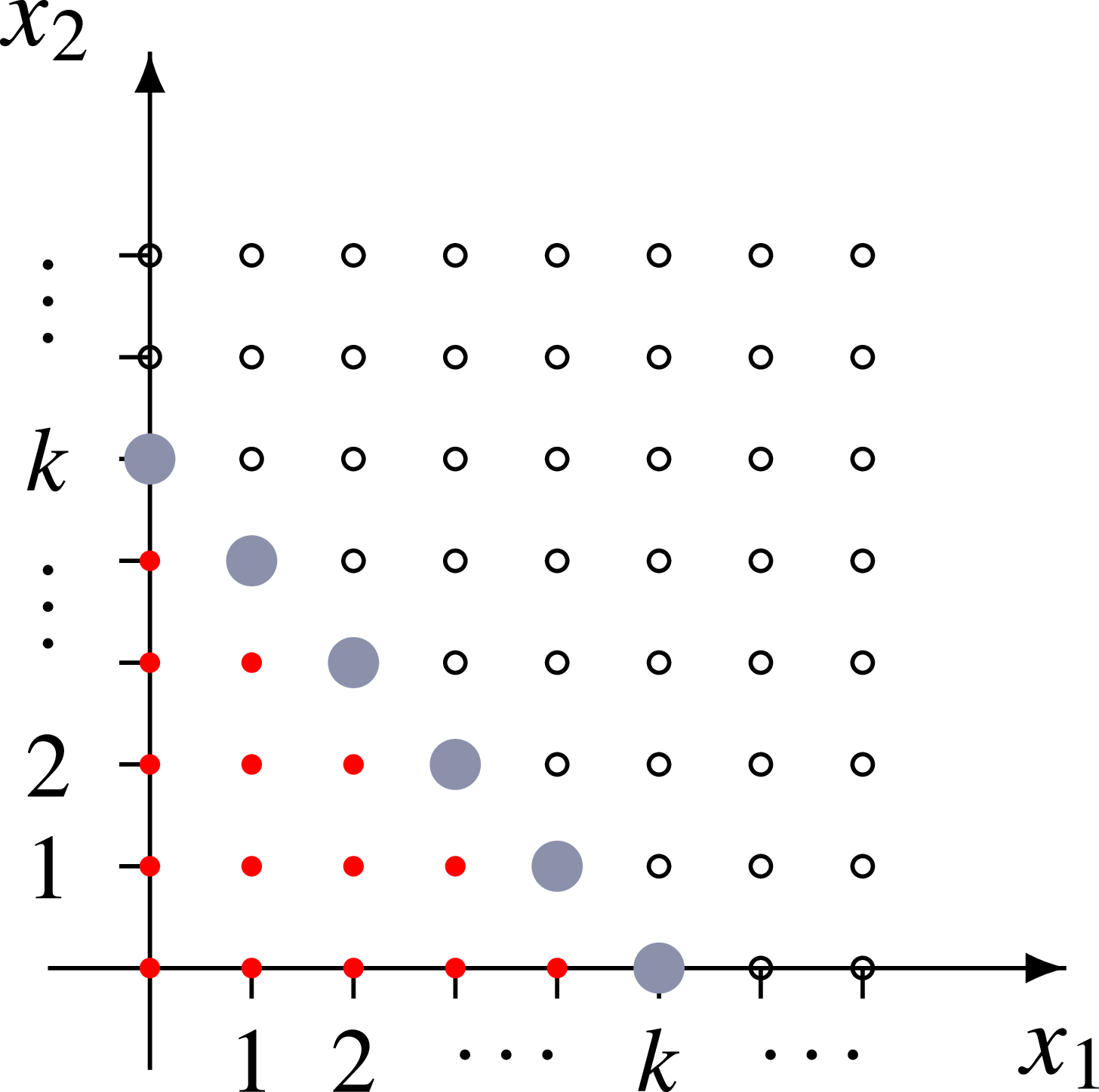
Example 1. Let M be a geometric distributed random variable with parameter $p\in(0,1)$
, i.e.
$p\in(0,1)$
, i.e. $p_M(k)=p(1-p)^{k-1}$
for
$p_M(k)=p(1-p)^{k-1}$
for $k\in\mathbb{N}$
. From (21), by applying the arithmetic–geometric series
$k\in\mathbb{N}$
. From (21), by applying the arithmetic–geometric series
 $$\sum_{k=0}^{+\infty} (a + kr) y^k = \frac{a}{1 - y} + \frac{ry}{(1 - y)^2}$$
for $|y|<1$
, with a few calculations it follows that
$|y|<1$
, with a few calculations it follows that
 \begin{equation}f_T(t)=2p\left[\frac{\lambda_1}{(\lambda_1+2pt)^2}+\frac{\lambda_2}{(\lambda_2+2pt)^2}-\frac{\lambda_1+\lambda_2}{(\lambda_1+\lambda_2+2pt)^2}\right],\qquad t\ge 0.\end{equation}
Similarly, from (22), we have
 \begin{equation}\overline{F}_T(t)=\frac{\lambda_1}{\lambda_1+2pt}+\frac{\lambda_2}{\lambda_2+2pt}-\frac{\lambda_1+\lambda_2}{\lambda_1+\lambda_2+2pt},\qquad t\ge 0,\end{equation}
which is a generalized mixture between three Pareto type-II (Lomax) distributions, having the same unitary shape parameter and scale parameters $2p/\lambda_1, 2p/\lambda_2$
, and
$2p/\lambda_1, 2p/\lambda_2$
, and $2p/(\lambda_1+\lambda_2)$
, respectively. We recall that the generalized mixtures are defined as the classic ones but they might contain negative coefficients, as in (25). Moreover, from (23), it holds that
$2p/(\lambda_1+\lambda_2)$
, respectively. We recall that the generalized mixtures are defined as the classic ones but they might contain negative coefficients, as in (25). Moreover, from (23), it holds that
 \begin{equation}h_T(t)=\frac{2p}{2pt + \lambda_1} + \frac{2p}{2pt + \lambda_2} + \frac{2p}{2pt + \lambda_1 + \lambda_2} - \frac{4p}{4pt + \lambda_1 + \lambda_2},\qquad t\ge 0.\end{equation}
In Figure 3 we plot the PDF $f_T$
given in (24) on the left-hand side, the SF
$f_T$
given in (24) on the left-hand side, the SF $\overline{F}_T$
given in (25) in the middle, and the hazard rate function
$\overline{F}_T$
given in (25) in the middle, and the hazard rate function $h_T(t)$
given in (26) on the right-hand side for suitable choices of the parameters
$h_T(t)$
given in (26) on the right-hand side for suitable choices of the parameters $\lambda_1,\lambda_2>0$
and
$\lambda_1,\lambda_2>0$
and $p\in(0,1)$
.
$p\in(0,1)$
.
Note that, from Example 1, the random thresholds considered in Figure 3 are ordered in the usual stochastic sense. Then, according to Remark 1, the corresponding random lifetimes are ordered in the usual stochastic sense too. Moreover, the hazard rate functions depicted on the right-hand side in Figure 3 are decreasing in $t\ge 0$
. Then the corresponding random lifetimes possess the property of decreasing failure rate (DFR); see, for instance, Section 4 in [Reference Navarro30]. In addition, we recall that the reversed hazard (or failure) rate function of a random lifetime T is defined by
$t\ge 0$
. Then the corresponding random lifetimes possess the property of decreasing failure rate (DFR); see, for instance, Section 4 in [Reference Navarro30]. In addition, we recall that the reversed hazard (or failure) rate function of a random lifetime T is defined by
 \begin{equation}\tilde{h}_T(t)\;:\!=\;\lim_{\varepsilon \to 0^+} \frac{\mathbb{P}(t - \varepsilon< T\le t \mid T \le t)}{\varepsilon}=\frac{f_T(t)}{1-\overline{F}_T(t)}\end{equation}
for all t such that $\overline{F}_T(t)<1$
, representing the instantaneous probability of failure at t for an item that has failed in the interval [0, t] (see Section 2.2 in [Reference Navarro30]). Hence, since the PDFs depicted on the left-hand side in Figure 3 are decreasing in
$\overline{F}_T(t)<1$
, representing the instantaneous probability of failure at t for an item that has failed in the interval [0, t] (see Section 2.2 in [Reference Navarro30]). Hence, since the PDFs depicted on the left-hand side in Figure 3 are decreasing in $t\ge 0$
, the corresponding random lifetimes have the property of decreasing reversed failure rate (DRFR); see, for instance, Section 4 in [Reference Navarro30].
$t\ge 0$
, the corresponding random lifetimes have the property of decreasing reversed failure rate (DRFR); see, for instance, Section 4 in [Reference Navarro30].


Note that, from (23) and (27), if T is DFR, then it is also DRFR. In general, the reverse implication does not hold. Indeed, in the next example, we consider a suitable choice for the random threshold M such that the corresponding random lifetime T is DRFR but not DFR. In this case the hazard rate function turns out to be increasing up to an instant close to 0, representing a high probability of an item’s failure when it starts working.
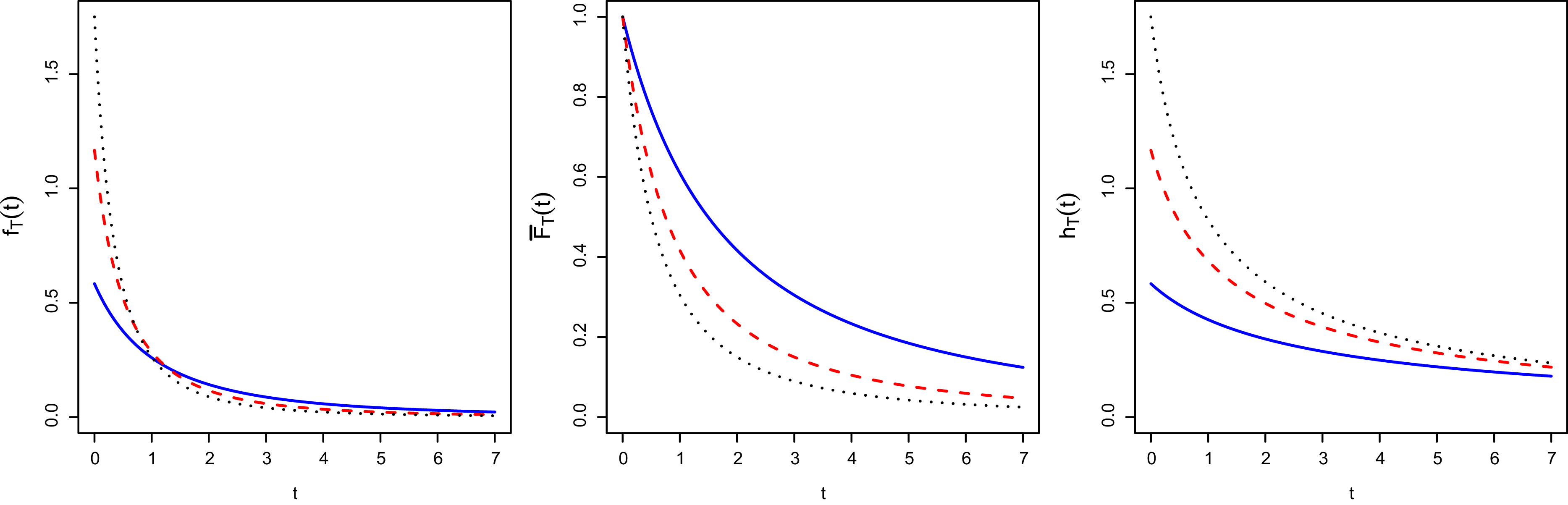
Example 2. Let M be uniformly distributed with $p_M(k)=1/3$
for
$p_M(k)=1/3$
for $k=1,2,3$
. Then, from (21), it follows that
$k=1,2,3$
. Then, from (21), it follows that
 \begin{equation}\begin{aligned}f_T(t)&=8 t^2 \left(\frac{\lambda_1}{(2 t + \lambda_1)^4}+ \frac{\lambda_2}{(2 t + \lambda_2)^4}- \frac{\lambda_1 + \lambda_2}{(2 t + \lambda_1 + \lambda_2)^4}\right)\\[3pt] &\quad+ \frac{8}{3} t \left(\frac{\lambda_1}{(2 t + \lambda_1)^3}+ \frac{\lambda_2}{(2 t + \lambda_2)^3}- \frac{\lambda_1 + \lambda_2}{(2 t + \lambda_1 + \lambda_2)^3}\right)\\[3pt] &\quad+ \frac{2}{3} \left(\frac{\lambda_1}{(2 t + \lambda_1)^2}+ \frac{\lambda_2}{(2 t + \lambda_2)^2}- \frac{\lambda_1 + \lambda_2}{(2 t + \lambda_1 + \lambda_2)^2}\right)\end{aligned}\end{equation}
for $t\ge 0$
, and, from (22), we get
$t\ge 0$
, and, from (22), we get
 \begin{equation}\begin{aligned}\overline{F}_T(t)&=\frac{\lambda_1}{2 t + \lambda_1} + \frac{\lambda_2}{2 t + \lambda_2} - \frac{\lambda_1 + \lambda_2}{2 t + \lambda_1 + \lambda_2} \\[5pt] &\quad+ \frac{4}{3} t^2 \left(\frac{\lambda_1}{(2 t + \lambda_1)^3} + \frac{\lambda_2}{(2 t + \lambda_2)^3} - \frac{\lambda_1 + \lambda_2}{(2 t + \lambda_1 + \lambda_2)^3}\right)\\[5pt] &\quad+ \frac{4}{3} t \left(\frac{\lambda_1}{(2 t + \lambda_1)^2} + \frac{\lambda_2}{(2 t + \lambda_2)^2} - \frac{\lambda_1 + \lambda_2}{(2 t + \lambda_1 + \lambda_2)^2}\right) \end{aligned}\end{equation}
for $t\ge 0$
. In Figure 4, for
$t\ge 0$
. In Figure 4, for $\lambda_1=5$
and
$\lambda_1=5$
and $\lambda_2=2$
, we plot the PDF
$\lambda_2=2$
, we plot the PDF $f_T$
given in (28) on the left-hand side, the SF
$f_T$
given in (28) on the left-hand side, the SF $\overline{F}_T$
given in (29) in the middle, and the corresponding hazard rate function
$\overline{F}_T$
given in (29) in the middle, and the corresponding hazard rate function

on the right-hand side, having used (23).
We conclude this section by providing an example in which M is a degenerate random variable, describing the case in which the sum of shocks that determines the item’s failure is fixed.


Example 3. Let M be a degenerate random variable in $k=2$
, i.e.
$k=2$
, i.e. $p_M(2)=1$
and
$p_M(2)=1$
and $p_M(k)=0$
for
$p_M(k)=0$
for $k\in\mathbb{N}\setminus{\{2\}}$
. Then, from (21), we have
$k\in\mathbb{N}\setminus{\{2\}}$
. Then, from (21), we have
 \begin{equation}f_T(t)=\frac{8\lambda_1t}{(2t + \lambda_1)^3}+ \frac{8\lambda_2t}{(2t + \lambda_2)^3}- \frac{8(\lambda_1 + \lambda_2)t}{(2t + \lambda_1 + \lambda_2)^3},\qquad t\ge 0,\end{equation}
and from (22) it holds that
 \begin{equation}\overline{F}_T(t)=\frac{\lambda_1 (4t + \lambda_1)}{(2t + \lambda_1)^2}- \frac{4t^2}{(2t + \lambda_2)^2}+ \frac{4t^2}{(2t + \lambda_1 + \lambda_2)^2},\qquad t\ge 0.\end{equation}
In Figure 5, for $\lambda_1=\lambda_2=2$
, we plot the (unimodal) PDF
$\lambda_1=\lambda_2=2$
, we plot the (unimodal) PDF $f_T$
given in (31) on the left-hand side, the SF
$f_T$
given in (31) on the left-hand side, the SF $\overline{F}_T$
given in (32) in the middle, and the corresponding hazard rate function
$\overline{F}_T$
given in (32) in the middle, and the corresponding hazard rate function
 \begin{equation}h_T(t)=\frac{2t\left(7+ 3t(3+t)\right)}{(1+t)(2+t)(2+3t(2+t))},\qquad t\ge 0,\end{equation}
on the right-hand side, having used (23).
5. Concluding Remarks and Future Developments
Shock models describe how systems or living organisms fail due to random stresses over time. An item starts working and experiences random shocks, with failure that occurs after a random number of these shocks. The geometric counting process represents a relevant option in the context of counting processes in order to handle random occurrences between events that are not independent. In this article shock models driven by the bivariate geometric counting process have been studied within a competing risks framework. We assume that the mixing distribution is given by the maximum of two independent exponential distributions. In addition, the dependence between the marginal geometric counting processes comes from the hypothesis that intensities of baseline Poisson processes are shared. We have assumed that the failures are due to one of two mutually exclusive causes. In particular, failures occur at the first instant in which a random threshold M is reached by a suitable function $\Psi$
of the two type of shock, given in (1). Under these assumptions we have obtained FDs, SFs, the probability of the cause of failure, and the moments of the failure time conditioned on a specific cause. Moreover, these functions have been laid down by considering
$\Psi$
of the two type of shock, given in (1). Under these assumptions we have obtained FDs, SFs, the probability of the cause of failure, and the moments of the failure time conditioned on a specific cause. Moreover, these functions have been laid down by considering $\Psi(x_1,x_2)=x_1+x_2$
. Particular cases have been analyzed for fixed distributions of M.
$\Psi(x_1,x_2)=x_1+x_2$
. Particular cases have been analyzed for fixed distributions of M.


Other functions $\Psi$
can be considered as long as they create certain partitions of the state space analogous to (1), such as (i)
$\Psi$
can be considered as long as they create certain partitions of the state space analogous to (1), such as (i) $\Psi(x_1,x_2)=\min\{x_1,x_2\}$
and (ii)
$\Psi(x_1,x_2)=\min\{x_1,x_2\}$
and (ii) $\Psi(x_1, x_2)=\max\{x_1,x_2\}$
. In addition, aiming to deal with more general settings, we can make alternative choices of counting processes that govern the shocks as well (see [Reference Cha and Finkelstein9, Reference Meoli28]). Note that each shock can be governed by a different type of counting process (for instance, one by the Poisson counting process and the other by the geometric counting process).
$\Psi(x_1, x_2)=\max\{x_1,x_2\}$
. In addition, aiming to deal with more general settings, we can make alternative choices of counting processes that govern the shocks as well (see [Reference Cha and Finkelstein9, Reference Meoli28]). Note that each shock can be governed by a different type of counting process (for instance, one by the Poisson counting process and the other by the geometric counting process).
Further dependency structures related to the counting processes involved can be considered and described by copulas (see, for instance, [Reference Durante and Sempi18]).
Another option for future research would be to develop a comprehensive inferential framework for the proposed shock models within competing risks, including methods for parameter estimation, model validation, and statistical testing.
Finally, the proposed competing risks model can be extended to the case of an arbitrary number r of types of shock. Let $(N_1(t),\ldots,N_r(t))$
be a multidimensional counting process, where
$(N_1(t),\ldots,N_r(t))$
be a multidimensional counting process, where $N_i(t)$
describes the number of shocks of the ith type that occurred in [0, t] for
$N_i(t)$
describes the number of shocks of the ith type that occurred in [0, t] for $i=1,2,\ldots,r$
. Then the SF of T can be expressed as
$i=1,2,\ldots,r$
. Then the SF of T can be expressed as
 $$\overline F_T(t)=\sum_{k=0}^{+\infty} p_M(k)\,\mathbb{P}\{\overline{\Psi}(N_1(t),\dots,N_r(t))<k\},\qquad t\geq 0,$$
where $\overline{\Psi}$
extends the function
$\overline{\Psi}$
extends the function $\Psi$
defined in (1) to the case of r components.
$\Psi$
defined in (1) to the case of r components.
Acknowledgements
The authors thank two anonymous reviewers for their contribution to improve a previous version of this work. MC and SS are members of the Gruppo Nazionale Calcolo Scientifico, Istituto Nazionale di Alta Matematica (GNCS-INdAM).
Funding information
This work is partially supported by GNCS-INdAM under the project ‘Metodi analitici e computazionali per processi stocastici multidimensionali ed applicazioni’ (CUP E53C23001670001) and by the European Union NextGenerationEU through MUR-PRIN 2022 PNRR, project P2022XSF5H, ‘Stochastic Models in Biomathematics and Applications’.
Competing interests
There are no competing interests to declare that arose during the preparation of or the publication process for this article.


 fT
fT F¯T
F¯T hT(t)
hT(t) λ1=1
λ1=1 λ2=2
λ2=2 p=0.25
 p=0.5
p=0.5 p=0.75
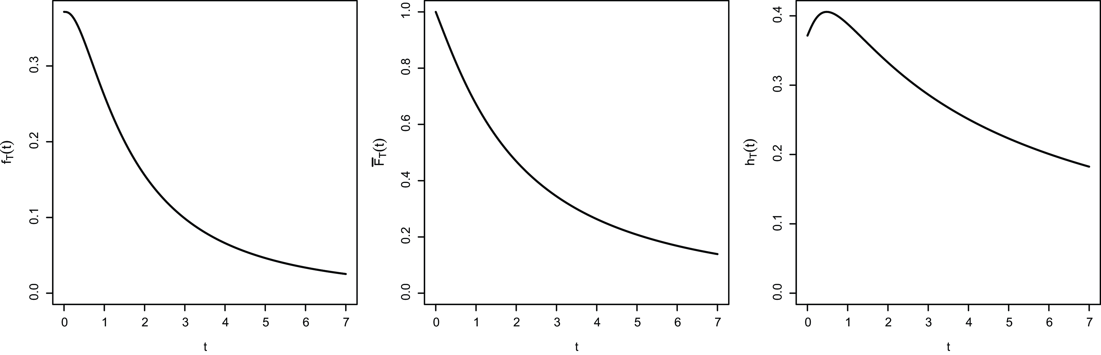
 fT
fT F¯T
F¯T hT(t)
hT(t) λ1=5
λ1=5 λ2=2
λ2=2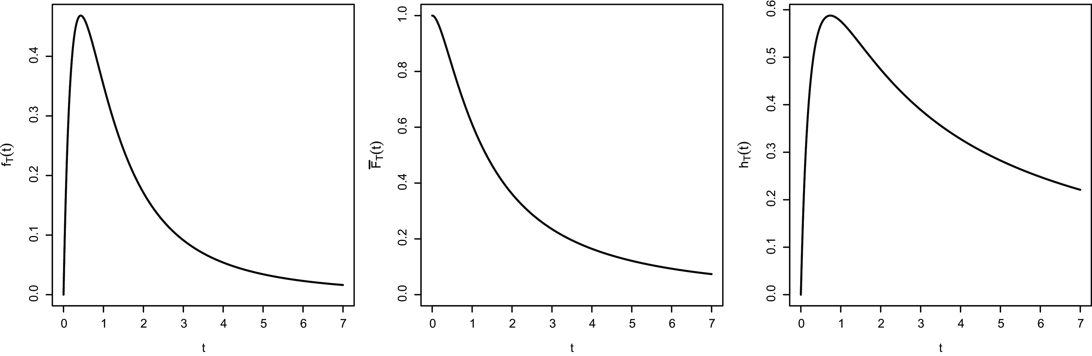
 fT
fT F¯T
F¯T hT(t)
hT(t) λ1=λ2=2
 Open access