





1 Introduction
Missing data are frequently encountered in the fields of education, psychology, and social science due to the nature of data collection through tests or questionnaires, where responses are often not mandatory (Rose et al., Reference Rose, von Davier and Nagengast2017; Yuan et al., Reference Yuan, Jamshidian and Kano2018). In timed tests, two types of missing behaviors can occur. One is called not-reached or dropout (Wu et al., Reference Wu, Chen, Schifano, Ibrahim and Fisher2019), where test takers fail to reach the end of the test due to time limits, early quitting, strategic planning, or other reasons. The other type is called omitted or intermittent missingness, where test takers skip questions intentionally or accidentally, or run out of time due to item-level time limits. For example, in the 2018 PISA math exam data in Brazil, 18.7% of test takers did not complete the test and 18.6% of answers was missing. Ignoring or handling missing data inappropriately can result in loss of information or even bias when analyzing the testing results (Glas & Pimentel, Reference Glas and Pimentel2008; Rose et al., Reference Rose, von Davier and Nagengast2015).
To appropriately address the missing data problem, one needs to understand different types of missing data mechanisms and their underlying assumptions. The term “ignorable” missingness was first introduced by Rubin (Reference Rubin1976), meaning that the inference for the response models is still valid if the missing data process is ignored. In contrast, missing data are considered nonignorable if Rubin’s assumption of ignorable missingness is violated (Little & Rubin, Reference Little and Rubin2019; Rabe-Hesketh & Skrondal, Reference Rabe-Hesketh and Skrondal2023). According to Glas and Pimentel (Reference Glas and Pimentel2008), Guo et al. (Reference Guo, Xu, Ying and Zhang2022), and Rose et al. (Reference Rose, von Davier and Nagengast2017), the not-reached and omitted behaviors may depend on the latent characteristics and the difficulty of the items and thus cannot be ignored for valid inference. The missingness is thus more likely to be nonignorable. Furthermore, these two behaviors are different processes that result in item nonresponses with different characteristics, and therefore should be handled differently in the item response theory (IRT) models (Rose, Reference Rose2013; Rose et al., Reference Rose, von Davier and Nagengast2017).
Approaches for dealing with the aforementioned nonignorable missingness for item responses have been developed. O’Muircheartaigh and Moustaki (Reference O’Muircheartaigh and Moustaki1999) proposed a shared parameter joint model for item responses and missing data indicators, where the tendency to omit items is included as a latent variable shared by both models. Following this framework, Holman and Glas (Reference Holman and Glas2005) considered a general IRT model framework via a combination of a generalized partial credit model (GPCM) for the observed dichotomous and polytomous responses and a multidimensional IRT (MIRT) model for the missing data process. Glas et al. (Reference Glas, Pimentel and Lamers2015) generalized the approach to incorporate covariates into the joint model of latent variables. For all the aforementioned papers, they focused only on missingness due to omission. Following the modeling framework of Holman and Glas (Reference Holman and Glas2005), Glas and Pimentel (Reference Glas and Pimentel2008) assumed a sequential IRT model with linear restrictions for the missing data model of the not-reached behavior. List et al. (Reference List, Köller and Nagy2019) extended the model by applying a semiparametric approach to capture nonlinear relationships between the onset of the not-reached items and the characteristics of test takers. Both papers focused on the unobserved responses at the end of the response sequence (the not-reached item) and did not consider missingness due to omission. To account for both omitted and not-reached missing behaviors, Rose et al. (Reference Rose, von Davier and Nagengast2017) proposed a joint model that combines an MIRT model for response and omitted items, and a latent regression model (LRM) for latent variables with a function of the number of not-reached items as a predictor. Consequently, the not-reached behavior of test takers was not directly modeled. Guo (Reference Guo2019) and Zhang et al. (Reference Zhang, Lu and Zhang2025) proposed a selection model to jointly study the item response and the missing data, where the cumulative number of missing indicators and cumulative responses were used as covariates in the missing data model. Our model adopts the joint modeling philosophy, but extends it by differentiating between intermittent and not-reached missingness to account for their distinct underlying causes, and incorporating response time data to enhance the modeling of item response and missing data process.
The response time for each item can sometimes be easily collected because of the prevalence of computerized testing. Many recent developments incorporate this additional source of information in the analysis of missing item response data, with the hope of improving the estimation and inference of item parameters and subjects’ latent characteristics (Guo et al., Reference Guo, Xu, Ying and Zhang2022; Lu & Wang, Reference Lu and Wang2020; Lu et al., Reference Lu, Wang and Shi2023; Pohl et al., Reference Pohl, Ulitzsch and von Davier2019; Ulitzsch et al., Reference Ulitzsch, von Davier and Pohl2020c; Van der Linden, Reference Van der Linden2007). Pohl et al. (Reference Pohl, Ulitzsch and von Davier2019) adopted a hierarchical framework to jointly model response accuracy and response time, assuming that the missingness was caused solely by time limits, an assumption not applicable to our real data, where the median total time spent on the test for not-reached subjects (23.26 minutes) is far less than the test time limit (60 minutes). Ulitzsch et al. (Reference Ulitzsch, von Davier and Pohl2020c) adopted the speed and accuracy model proposed in Van der Linden (Reference Van der Linden2007) and the IRT model for the omitted behavior proposed in Holman and Glas (Reference Holman and Glas2005), and assumed different response time models for the observed and omitted items. Ulitzsch et al. (Reference Ulitzsch, von Davier and Pohl2020a) further included the modeling of engagement (guessing) behavior in the hierarchical model framework, and assumed fully engaged students did not skip questions. Both papers focused exclusively on omission behavior. Lu and Wang (Reference Lu and Wang2020) proposed a response time process (RTprocess) model where they modeled item omission as a type of censoring. They assumed that the omitted items were due to item-level time limits, and that the not-reached items were not the result of early quitting. Guo et al. (Reference Guo, Xu, Ying and Zhang2022) proposed a joint model for responses and response times that accounts for missingness due to the not-reached behavior, where a censoring mechanism was assumed for the response time. Similarly, the not-reached and omitted behaviors were not directly modeled. Lu et al. (Reference Lu, Wang and Shi2023) proposed a two-stage mixture RTprocess model to detect aberrant behaviors (i.e., cheating and guessing behaviors) and to account for item nonresponses (not-reached and omitted items). Their model did not differentiate between the not-reached and omitted behaviors and assumed that the missing data mechanism was ignorable if the response time information was incorporated. Ulitzsch et al. (Reference Ulitzsch, von Davier and Pohl2020b, Reference Ulitzsch, Alfers, Lu, Wang, Pohl, Khorramdel, von Davier and Yamamoto2025) proposed a model that accounts for different types of not-reached behaviors: a response time model to address not-reached behavior due to time limits, and a Poisson model to address not-reached behavior due to early quitting. Their paper centered solely on not-reached behavior. Ulitzsch et al. (Reference Ulitzsch, Zhang and Pohl2024) distinguished rapid omissions from omissions due to solution behavior and considered omission classification uncertainty. Their paper focused only on missingness due to omission. Guo et al. (Reference Guo, Xu, Fang, Ying and Zhang2025) proposed a joint model of item response, response time, and omitted time through the competing risk formulation. The three outcomes were assumed to be conditionally independent given the latent traits, where a multivariate normal distribution was adopted. Their paper focused on missingness due to omission only.
Not-reached and omitted behaviors often stem from different behavioral processes, such as time limits, early quitting, or strategic planning, which may follow distinct missing data mechanisms. These two types of behaviors should be modeled separately to capture their unique characteristics, but also jointly, as they may both be related to the same underlying latent ability and item difficulty parameters (Debeer et al., Reference Debeer, Janssen and De Boeck2017; Mislevy & Wu, Reference Mislevy and Wu1988). Joint modeling of both behaviors allows for a more accurate understanding of test-taking behavior and results in improved parameter estimation by borrowing information between both types of missing behaviors. Guo et al. (Reference Guo, Xu and Zhang2025) proposed a joint model framework for both omitted items and not-reached items by combining the competing risk models from Guo et al. (Reference Guo, Xu and Zhang2025) and the censoring approach introduced in Guo et al. (Reference Guo, Xu, Ying and Zhang2022). Their focus was on missingness resulting from time limits. The existing literature that simultaneously modeling both not-reached and omitted behaviors is sparse, and our study aims to fill this gap. In this article, we propose a joint model framework to simultaneously study the item response, response time, the not-reached missingness, and the omitted missingness, without restricting missingness to time constraints. Specifically, a summary of the contributions of this work is listed below.
-
(i) A data-driven missing data model is developed to allow for joint modeling of the not-reached and omitted behaviors of test takers. Specifically, a sequential multinomial model is developed for the not-reached behavior, and a conditional model is proposed for the omitted behavior given the not-reached behavior. This formulation enables the modeling of not-reached and omission behaviors within a unified IRT modeling framework. It also provides a clear and natural distinction between the two types of missing behaviors: the omitted behavior, which may be due to strategic planning, and the not-reached behavior, which may be due to early quitting or time limits. Our proposed missing data model assumes nonignorable because the probability of missingness does not directly depend on any unobserved data but only depends on latent variables, and the missing data process cannot be ignored for valid inference of the response models (Pohl & Becker, Reference Pohl and Becker2020; Robitzsch, Reference Robitzsch2021, Reference Robitzsch2023). The model also encompasses an ignorable missing data mechanism as a special case.
-
(ii) We propose a hierarchical model framework and a new formulation for the joint distributions of all latent propensity parameters. This allows us to quantify the extent to which the missing data mechanism is nonignorable and to conveniently incorporate the conditional independence properties of latent propensity parameters, facilitating the specification of prior distributions more conveniently and resulting in a more efficient implementation and better mixing of Markov chain Monte Carlo (MCMC) sampling. Our simulation studies demonstrate good empirical performances even when the missing data percentages are as small as 5%, either due to omission or due to not-reached behaviors.
-
(iii) The decomposition techniques of various model selection criteria have been widely applied to the IRT to enhance the understanding of model fit within the joint model framework (Liu et al., Reference Liu, Chen, Wang and Hancock2025; Sun et al., Reference Sun, Liu, Wang and Chen2025). In this article, we also develop a model selection criterion, built on the decomposition of the logarithm of the pseudo marginal likelihood (LPML), a computationally efficient posterior predictive criterion, using the idea of leave-one-subject-out. The decomposition of LPML gatekeeps the selection of the “best” missing data mechanism. More importantly, it can also be used to quantify the importance of modeling the item response and response time jointly versus individually in identifying the missing data mechanism.
The remainder of this article is organized as follows. We present models for the item response, response time, and missing data mechanism in Section 2. The hierarchical model framework and Bayesian inference are given in Sections 3 and 4, including the decomposition of LPML for model fit assessment. Extensive simulation studies and a detailed analysis of the PISA 2018 data are presented in Sections 5 and 6, respectively. Finally, we conclude this article with a brief discussion in Section 7.
2 Models
2.1 Item response model
Suppose that there are a total of n subjects and J items. Let
$y_{ij}$
 denote the binary score for the i
th
subject at item j, where
$y_{ij}=1$
denote the binary score for the i
th
subject at item j, where
$y_{ij}=1$
 indicates that the answer is correct and
$y_{ij}=0$
indicates that the answer is correct and
$y_{ij}=0$
 otherwise. Denoting
$P(y_{ij}=1)=p_{y_{ij}}$
otherwise. Denoting
$P(y_{ij}=1)=p_{y_{ij}}$
 , a two-parameter logistic model (2PL) (Bock & Aitkin, Reference Bock and Aitkin1981) is assumed for
$p_{y_{ij}}$
, a two-parameter logistic model (2PL) (Bock & Aitkin, Reference Bock and Aitkin1981) is assumed for
$p_{y_{ij}}$
 as
as

for
$ i=1, \dots , n, j=1, \dots , J$
 , where
$\mathbf {{{a}}}_Y=(a_{Y1}, \dots , a_{YJ})^{'}$
, where
$\mathbf {{{a}}}_Y=(a_{Y1}, \dots , a_{YJ})^{'}$
 is the vector of discrimination parameters,
${{\boldsymbol{\theta }}_Y}=(\theta _{Y1}, \dots , \theta _{Yn})^{'}$
is the vector of discrimination parameters,
${{\boldsymbol{\theta }}_Y}=(\theta _{Y1}, \dots , \theta _{Yn})^{'}$
 is the vector of latent response propensity parameters (O’Muircheartaigh & Moustaki, Reference O’Muircheartaigh and Moustaki1999) measuring the tendency to give correct answers, and
$\mathbf{b}_Y=(b_{Y1}, \dots , b_{YJ})^{'}$
is the vector of latent response propensity parameters (O’Muircheartaigh & Moustaki, Reference O’Muircheartaigh and Moustaki1999) measuring the tendency to give correct answers, and
$\mathbf{b}_Y=(b_{Y1}, \dots , b_{YJ})^{'}$
 is the vector of difficulty parameters. A higher value of the product of
$a_{Yj}$
is the vector of difficulty parameters. A higher value of the product of
$a_{Yj}$
 and
$b_{Yj}$
and
$b_{Yj}$
 indicates that the corresponding item j is more difficult and, consequently, the answer is more likely to be wrong.
2.2 Response time model
Let
$t_{ij}$
 denote the response time for the i
th
subject at item j. A log-normal model (Van der Linden, Reference Van der Linden2006, Reference Van der Linden2007) is built as
denote the response time for the i
th
subject at item j. A log-normal model (Van der Linden, Reference Van der Linden2006, Reference Van der Linden2007) is built as

where
$\mathbf {{{b}}}_{T}=(b_{T1}, \dots , b_{TJ})^{'}$
 is the vector of time intensity parameters,
${{ {\theta }}}_{T}=(\theta _{T1}, \dots $
is the vector of time intensity parameters,
${{ {\theta }}}_{T}=(\theta _{T1}, \dots $
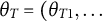 ,
$ \theta _{Tn})^{'}$
,
$ \theta _{Tn})^{'}$
 is the vector of latent response time propensity parameters,
$\sigma _T>0$
is the vector of latent response time propensity parameters,
$\sigma _T>0$
 captures the subject-specific variation,
$\epsilon _{ij} \sim N(0, \frac {1}{a_{Tj}})$
captures the subject-specific variation,
$\epsilon _{ij} \sim N(0, \frac {1}{a_{Tj}})$
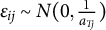 , and
$\mathbf {{{a}}}_{T}=(a_{T1}, \dots $
, and
$\mathbf {{{a}}}_{T}=(a_{T1}, \dots $
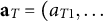 ,
$a_{TJ})^{'}$
,
$a_{TJ})^{'}$
 is the vector of precision parameters. A higher value of
$b_{Tj}$
is the vector of precision parameters. A higher value of
$b_{Tj}$
 indicates that subjects tend to take more time on item j.
2.3 Missing data models
We adopt a sequential multinomial model to study the not-reached behavior of each subject. A joint model of all the previous missing statuses, that is, omitted behavior, is then developed given that the subject fails to reach a certain item.
Let
$W_i$
 denote the item number at which the i
th
subject fails to reach, for
$i=1, \dots , n$
denote the item number at which the i
th
subject fails to reach, for
$i=1, \dots , n$
 . The possible values of
$W_i$
. The possible values of
$W_i$
 are
$1,2,\dots , J, J+1$
are
$1,2,\dots , J, J+1$
 , where
$W_i=J+1$
, where
$W_i=J+1$
 indicates that the i
th
subject reaches the last item.
indicates that the i
th
subject reaches the last item.
Let

We then have

A Rasch model (Rasch, Reference Rasch1993) is assumed for
$p_{ij}$
 in (3):

for
$i=1, \dots , n, j=1, \dots , J$
 . Let
${{ {\theta }}}_W=(\theta _{W1}, \dots , \theta _{Wn})'$
. Let
${{ {\theta }}}_W=(\theta _{W1}, \dots , \theta _{Wn})'$
 denote the vector of latent not-reached propensity parameters (O’Muircheartaigh & Moustaki, Reference O’Muircheartaigh and Moustaki1999; Ulitzsch et al., Reference Ulitzsch, von Davier and Pohl2020a) that measure the tendency to withdraw from the test and
$\mathbf {{{b}}}_W=(b_{W1}, \dots , b_{WJ})'$
denote the vector of latent not-reached propensity parameters (O’Muircheartaigh & Moustaki, Reference O’Muircheartaigh and Moustaki1999; Ulitzsch et al., Reference Ulitzsch, von Davier and Pohl2020a) that measure the tendency to withdraw from the test and
$\mathbf {{{b}}}_W=(b_{W1}, \dots , b_{WJ})'$
 denote the vector of difficulty parameters for the not-reached behavior. This allows us to model the not-reached behavior within a unified IRT modeling framework.
Let
$R_{i\ell }$
 be the binary variable that indicates whether item
$\ell $
be the binary variable that indicates whether item
$\ell $
 is omitted or not for the i
th
subject:
is omitted or not for the i
th
subject:

Assuming that the i
th
subject fails to reach item j (
$W_i=j$
 ), we know for sure that the missing indicator
$R_{i\ell }=1$
), we know for sure that the missing indicator
$R_{i\ell }=1$
 with probability one for
$\ell \ge j$
with probability one for
$\ell \ge j$
 . Moreover,
$y_{i,j-1}$
. Moreover,
$y_{i,j-1}$
 must be observed (
$R_{i,j-1}=0$
must be observed (
$R_{i,j-1}=0$
 ) with probability one. Otherwise,
$W_i < j$
) with probability one. Otherwise,
$W_i < j$
 , which contradicts the condition that
$W_i=j$
, which contradicts the condition that
$W_i=j$
 . Thus, given
$W_i=j$
. Thus, given
$W_i=j$
 , we only need to model the conditional joint distribution of
$R_{i\ell }$
, we only need to model the conditional joint distribution of
$R_{i\ell }$
 up to
$\ell =j-2$
up to
$\ell =j-2$
 .
.
Following Ibrahim, Chen, and Lipsitz (Reference Ibrahim, Chen and Lipsitz2001) and Ibrahim et al. (Reference Ibrahim, Chen, Lipsitz and Herring2005), we write the joint distribution of
$(R_{i1}, \dots , R_{ij-2})$
 through a sequence of one-dimensional conditional distributions. Specifically, for
$j=2$
through a sequence of one-dimensional conditional distributions. Specifically, for
$j=2$
 ,
$P(R_{i1}=r_{i1}|W_i=2)=1-r_{i1}$
,
$P(R_{i1}=r_{i1}|W_i=2)=1-r_{i1}$
 ; for
$j=3$
; for
$j=3$
 ,
$ P(R_{i1}=r_{i1}, R_{i2}=r_{i2}|W_i=3)= f(r_{i1}| W_i=3) (1-r_{i2}); $
,
$ P(R_{i1}=r_{i1}, R_{i2}=r_{i2}|W_i=3)= f(r_{i1}| W_i=3) (1-r_{i2}); $
 and for
$j> 3$
and for
$j> 3$
 ,
$ P(R_{i1}=r_{i1}, \dots , R_{i,j-2}=r_{i,j-2}|W_i=j)= f(r_{i1}| W_i=j) \prod _{\ell =2}^{j-2} f(r_{i\ell }| W_i=j, r_{i1}, \dots ,r_{i,\ell -1})$
,
$ P(R_{i1}=r_{i1}, \dots , R_{i,j-2}=r_{i,j-2}|W_i=j)= f(r_{i1}| W_i=j) \prod _{\ell =2}^{j-2} f(r_{i\ell }| W_i=j, r_{i1}, \dots ,r_{i,\ell -1})$
 . We assume the following formulation for the conditional distribution of
$R_{i\ell }$
. We assume the following formulation for the conditional distribution of
$R_{i\ell }$
 given
$W_i=j$
given
$W_i=j$
 and the previous omitted indicators:

where
$q_{i\ell }$
 is modeled by another Rasch model:

for
$i=1, \dots , n, \ell =1, \dots , j-2$
 . Let
${{ {\theta }}}_R=(\theta _{R1}, \dots , \theta _{Rn})'$
. Let
${{ {\theta }}}_R=(\theta _{R1}, \dots , \theta _{Rn})'$
 denote the vector of latent omission propensity parameters that measures the tendency to omit the item, and
$\mathbf {{{b}}}_R=(b_{R1}, \dots , b_{R,J-1})'$
denote the vector of latent omission propensity parameters that measures the tendency to omit the item, and
$\mathbf {{{b}}}_R=(b_{R1}, \dots , b_{R,J-1})'$
 denote the vector of difficulty parameters for the omitted behavior model. A higher value of
$b_{R\ell }$
denote the vector of difficulty parameters for the omitted behavior model. A higher value of
$b_{R\ell }$
 indicates that the corresponding item
$\ell $
indicates that the corresponding item
$\ell $
 is less difficult and tends to be answered.
The joint distribution of
$W_i$
 and
$\mathbf {{{R}}}_i=(R_{i1}, \dots , R_{iJ})'$
and
$\mathbf {{{R}}}_i=(R_{i1}, \dots , R_{iJ})'$
 can be written as

Remark 2.1. The sequential model framework in (3) and (4) allows us to directly interpret
$p_{ij}=P(W_i=j|j \le W_i < J+1) $
 , that is, the chance of failing to reach the current item given that the subject has not withdrawn from the test. This is inspired by the survival function in survival analysis, where
$p_{ij}$
, that is, the chance of failing to reach the current item given that the subject has not withdrawn from the test. This is inspired by the survival function in survival analysis, where
$p_{ij}$
 is of great practical interest and should not depend on later items. The sequential model framework implicitly takes into account the order of items, where each
$p_{ij}$
is of great practical interest and should not depend on later items. The sequential model framework implicitly takes into account the order of items, where each
$p_{ij}$
 depends on the item values only up to j, rather than taking them as a whole in a conventional multinomial logistic regression model (Wu et al., Reference Wu, Chen, Schifano, Ibrahim and Fisher2019). This aligns well with the design of certain computer-based tests, such as PISA 2018, which do not allow students to return to a question once it has been answered or skipped. The proposed sequential logistic regression model is therefore more appealing. The sequential multinomial model for the not-reached behavior automatically sets the upper limit of the total number of not-reached items and allows for incorporating both subject-specific and item-specific parameters, which is expected to provide a better fit for the data than a more parsimonious Poisson model in Ulitzsch et al. (Reference Ulitzsch, von Davier and Pohl2020b, Reference Ulitzsch, Alfers, Lu, Wang, Pohl, Khorramdel, von Davier and Yamamoto2025).
Remark 2.2. The minimum requirements for the missing data models in (5) and (7) to be estimated are that i) the number of subjects failing to reach item j should be greater than 0 for any j and ii) the number of omissions should be greater than 0 for any item level. These conditions are akin to the traditional requirement of “adequate item response variability” in response models (Hambleton et al., Reference Hambleton, Swaminathan and Rogers1991). In Section 3, we introduce a hierarchical framework where these requirements can be relaxed by borrowing information from items with missing data. Apart from the traditional assumptions for IRT models (Fox, Reference Fox2010), the only additional assumption introduced to simplify the proposed missing data model is given in Equation (6):
$R_{i\ell }$
 is independent of
$W_i$
is independent of
$W_i$
 given
$(R_{i1}, \dots , R_{i,\ell -1})$
given
$(R_{i1}, \dots , R_{i,\ell -1})$
 . This assumption can potentially be relaxed if there is evidence that
$P(R_{i\ell }=1| W_i=j, R_{i1}=r_{i1}, \dots , R_{i,\ell -1}=r_{i,\ell -1})$
. This assumption can potentially be relaxed if there is evidence that
$P(R_{i\ell }=1| W_i=j, R_{i1}=r_{i1}, \dots , R_{i,\ell -1}=r_{i,\ell -1})$
 varies between different item levels, with a sufficiently large percentage of missing data and a sufficiently large sample size n, and a sufficiently small number of items J. Additionally, we assume that
$q_{i\ell }$
varies between different item levels, with a sufficiently large percentage of missing data and a sufficiently large sample size n, and a sufficiently small number of items J. Additionally, we assume that
$q_{i\ell }$
 does not depend on any function of
$R_{ij}, j=1, \dots , \ell -1$
does not depend on any function of
$R_{ij}, j=1, \dots , \ell -1$
 for better identifiability. This assumption can also be relaxed with a large enough percentage of missing data and a large enough sample size (Köhler et al., Reference Köhler, Pohl and Carstensen2015).
3 Hierarchical model framework
3.1 Latent propensity parameters
For the i
th
subject, let
$\mathbf {{{y}}}_{i}=(y_{i1},\dots ,y_{iJ})'$
 denote the vector of all response measures and
$\mathbf {{t}}_{i}=(t_{i1},\dots ,t_{iJ})'$
denote the vector of all response measures and
$\mathbf {{t}}_{i}=(t_{i1},\dots ,t_{iJ})'$
 denote the vector of all response times. Let
$\mathbf {{{y}}}=(\mathbf {{{y}}}_1', \dots , \mathbf {{{y}}}_n')'$
denote the vector of all response times. Let
$\mathbf {{{y}}}=(\mathbf {{{y}}}_1', \dots , \mathbf {{{y}}}_n')'$
 ,
$\mathbf {{t}}=(\mathbf {{t}}_1', \dots , \mathbf {{t}}_n')'$
,
$\mathbf {{t}}=(\mathbf {{t}}_1', \dots , \mathbf {{t}}_n')'$
 ,
$\mathbf {{W}}=(W_1, \dots , W_n)'$
,
$\mathbf {{W}}=(W_1, \dots , W_n)'$
 , and
$\mathbf {{{R}}}=(\mathbf {{{R}}}_1', \dots , \mathbf {{{R}}}_n')'$
, and
$\mathbf {{{R}}}=(\mathbf {{{R}}}_1', \dots , \mathbf {{{R}}}_n')'$
 . To capture the dependence between
$\mathbf {{{y}}}$
. To capture the dependence between
$\mathbf {{{y}}}$
 ,
$\mathbf {{t}}$
,
$\mathbf {{t}}$
 ,
$\mathbf {{W}}$
,
$\mathbf {{W}}$
 , and
$\mathbf {{{R}}}$
, and
$\mathbf {{{R}}}$
 , we assume the following joint distributions of the latent propensity parameters:

where
$\boldsymbol {\mu }$
 is a four-dimensional column vector and
$\Sigma $
is a four-dimensional column vector and
$\Sigma $
 is the covariance matrix of
$({\theta _{Yi}}, \theta _{Ti}, \theta _{Wi}, \theta _{Ri})'$
is the covariance matrix of
$({\theta _{Yi}}, \theta _{Ti}, \theta _{Wi}, \theta _{Ri})'$
 given by

To ensure identifiability, let
$\boldsymbol {\mu }$
 be a four-dimensional column vector of zeros and the diagonal elements of
$\Sigma $
be a four-dimensional column vector of zeros and the diagonal elements of
$\Sigma $
 be 1.
be 1.
Proposition 3.1. For
$i=1, \dots , n$
 ,
$\theta _{Wi}$
,
$\theta _{Wi}$
 and
$\theta _{Ri}$
and
$\theta _{Ri}$
 are conditionally independent given
${\theta _{Yi}}$
are conditionally independent given
${\theta _{Yi}}$
 and
$\theta _{Ti}$
and
$\theta _{Ti}$
 if and only if

Proof of Proposition 3.1
For multivariate normal distributions, uncorrelated and independent properties are equivalent. Thus, we focus on the conditional covariance matrix of
$( \theta _W, \theta _{Ri})' |({\theta _{Yi}}, \theta _{Ti})'$
 , which is given by

where

Therefore,
$\theta _{Wi}$
 and
$\theta _{Ri}$
and
$\theta _{Ri}$
 are conditionally independent given
${\theta _{Yi}}$
are conditionally independent given
${\theta _{Yi}}$
 if and only if
$\text {Cov}(\theta _{Wi}, \theta _{Ri}|{\theta _{Yi}}, \theta _{Ti})=\Sigma _{12}=0$
if and only if
$\text {Cov}(\theta _{Wi}, \theta _{Ri}|{\theta _{Yi}}, \theta _{Ti})=\Sigma _{12}=0$
 .
.
Proposition 3.1 leads to the following formulation:

where
$\eta _{T} \in (-1, 1)$
 ,
$\zeta _{Ti} \sim N(0, 1)$
,
$\zeta _{Ti} \sim N(0, 1)$
 ,
$\eta _W \in (-1, 1)$
,
$\eta _W \in (-1, 1)$
 ,
$\alpha _W \in (0, \pi ]$
,
$\alpha _W \in (0, \pi ]$
 ,
$\zeta _{Wi} \sim N(0, 1)$
,
$\zeta _{Wi} \sim N(0, 1)$
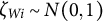 ,
$\eta _R \in (-1, 1)$
,
$\eta _R \in (-1, 1)$
 ,
$\alpha _R \in (0, \pi ]$
,
$\alpha _R \in (0, \pi ]$
 ,
$\zeta _{Ri} \sim N(0, 1)$
,
$\zeta _{Ri} \sim N(0, 1)$
 , and
$\zeta _{Ti}$
, and
$\zeta _{Ti}$
 ,
$\zeta _{Wi} , \zeta _{Ri}$
,
$\zeta _{Wi} , \zeta _{Ri}$
 are independent of
${\theta _{Yi}}$
are independent of
${\theta _{Yi}}$
 , for
$i=1, \dots , n$
, for
$i=1, \dots , n$
 . It is worth noting that
$(\eta _W, \alpha _W)$
. It is worth noting that
$(\eta _W, \alpha _W)$
 and
$(\eta _R, \alpha _R)$
and
$(\eta _R, \alpha _R)$
 can be viewed as polar coordinate systems.
In this formulation,
${{\boldsymbol {\mu }}}=(0, 0, 0, 0)'$
 and
$\Sigma $
and
$\Sigma $
 are given by

where

After some algebra, we can show that condition (10) in Proposition 3.1 is satisfied and consequently
$\theta _{Wi}$
 and
$\theta _{Ri}$
and
$\theta _{Ri}$
 are conditionally independent given
${\theta _{Yi}}$
are conditionally independent given
${\theta _{Yi}}$
 and
$\theta _{Ti}$
and
$\theta _{Ti}$
 for any i.
Remark 3.1. To guarantee that the matrix in (12) is positive definite, we need to ensure that all the leading principal minors of the matrix are positive. After some algebra, we obtain the
$1\times 1$
 ,
$2\times 2$
,
$2\times 2$
 ,
$3\times 3$
,
$3\times 3$
 , and
$4\times 4$
, and
$4\times 4$
 leading principal minors: 1,
$1-\eta _T^2$
leading principal minors: 1,
$1-\eta _T^2$
 ,
$(1-\eta _T^2)(1-\eta _W^2)$
,
$(1-\eta _T^2)(1-\eta _W^2)$
 , and
$(1-\eta _T^2)(1-\eta _W^2)(1-\eta _R^2)$
, and
$(1-\eta _T^2)(1-\eta _W^2)(1-\eta _R^2)$
 . All are positive since
$\eta _T, \eta _W, \eta _R \in (-1, 1)$
. All are positive since
$\eta _T, \eta _W, \eta _R \in (-1, 1)$
 . Thus, we can assign independent priors to these parameters, since there are no constraints between them. Compared with the original joint distribution in (8) and (9), which requires additional constraints on the parameters to ensure positive definiteness, the current formulation induced by conditional independence in (11) and (12) results in a more efficient implementation and better mixing of MCMC sampling.
Remark 3.2. Let
$\mathbf {{{y}}}_{\mathrm {obs}}=(\mathbf {{{y}}}^{\prime }_{1, \mathrm {obs}}, \dots , \mathbf {{{y}}}^{\prime }_{n, \mathrm {obs}})'$
 and
$\mathbf {{{y}}}_{\mathrm {mis}}=(\mathbf {{{y}}}^{\prime }_{1, \mathrm {mis}}, \dots , \mathbf {{{y}}}^{\prime }_{n, \mathrm {mis}})'$
and
$\mathbf {{{y}}}_{\mathrm {mis}}=(\mathbf {{{y}}}^{\prime }_{1, \mathrm {mis}}, \dots , \mathbf {{{y}}}^{\prime }_{n, \mathrm {mis}})'$
 , where
$\mathbf {{{y}}}_{i, \mathrm {obs}}$
, where
$\mathbf {{{y}}}_{i, \mathrm {obs}}$
 and
$\mathbf {{{y}}}_{i, \mathrm {mis}}$
and
$\mathbf {{{y}}}_{i, \mathrm {mis}}$
 are the observed and missing responses for the i
th
subject. Similarly, let
$\mathbf {{t}}_{\mathrm {obs}}=(\mathbf {{t}}^{\prime }_{1, \mathrm {obs}}, \dots , \mathbf {{t}}^{\prime }_{n, \mathrm {obs}})'$
are the observed and missing responses for the i
th
subject. Similarly, let
$\mathbf {{t}}_{\mathrm {obs}}=(\mathbf {{t}}^{\prime }_{1, \mathrm {obs}}, \dots , \mathbf {{t}}^{\prime }_{n, \mathrm {obs}})'$
 and
$\mathbf {{t}}_{\mathrm {mis}}=(\mathbf {{t}}^{\prime }_{1, \mathrm {mis}}, \dots , \mathbf {{t}}^{\prime }_{n, \mathrm {mis}})'$
and
$\mathbf {{t}}_{\mathrm {mis}}=(\mathbf {{t}}^{\prime }_{1, \mathrm {mis}}, \dots , \mathbf {{t}}^{\prime }_{n, \mathrm {mis}})'$
 , where
$(\mathbf {{t}}_{i, \mathrm {obs}}, \mathbf {{t}}_{i, \mathrm {mis}})$
, where
$(\mathbf {{t}}_{i, \mathrm {obs}}, \mathbf {{t}}_{i, \mathrm {mis}})$
 denote the response times for the observed and missing items, respectively, for the
$i^{\text {th}}$
denote the response times for the observed and missing items, respectively, for the
$i^{\text {th}}$
 subject, with the response times for the omitted items treated as missing data. Let
$\Omega _{YT}=(\mathbf {{{a}}}_Y, \mathbf {{{b}}}_Y, {\mathbf {{{a}}}_T}, \mathbf {{{b}}}_{T}, \eta _T)$
subject, with the response times for the omitted items treated as missing data. Let
$\Omega _{YT}=(\mathbf {{{a}}}_Y, \mathbf {{{b}}}_Y, {\mathbf {{{a}}}_T}, \mathbf {{{b}}}_{T}, \eta _T)$
 and
$\Omega _{WR}=( \mathbf {{{b}}}_W, \eta _W,\alpha _W, \mathbf {{{b}}}_R, \eta _R, \alpha _R)$
and
$\Omega _{WR}=( \mathbf {{{b}}}_W, \eta _W,\alpha _W, \mathbf {{{b}}}_R, \eta _R, \alpha _R)$
 denote the collections of parameters for the response models and missing data models, respectively. Let
$V_L$
denote the collections of parameters for the response models and missing data models, respectively. Let
$V_L$
 denote the collection of latent propensity variables, including
${{ {\theta }}}_i, \zeta _{Ti}, \zeta _{Wi}, \zeta _{Ri}, i=1, \dots , n$
denote the collection of latent propensity variables, including
${{ {\theta }}}_i, \zeta _{Ti}, \zeta _{Wi}, \zeta _{Ri}, i=1, \dots , n$
 .
.
As discussed in Ibrahim et al. (Reference Ibrahim, Chen, Lipsitz and Herring2005) and Wu et al. (Reference Wu, Chen, Schifano, Ibrahim and Fisher2019), after integrating
$V_L$
 , the missing data mechanism is ignorable if
$P(\mathbf {{W}}, \mathbf {{{R}}}|\mathbf {{{y}}}, \mathbf {{t}}, \Omega _{yT}, \Omega _{WR})= P(\mathbf {{W}}, \mathbf {{{R}}}| \Omega _{WR})$
, the missing data mechanism is ignorable if
$P(\mathbf {{W}}, \mathbf {{{R}}}|\mathbf {{{y}}}, \mathbf {{t}}, \Omega _{yT}, \Omega _{WR})= P(\mathbf {{W}}, \mathbf {{{R}}}| \Omega _{WR})$
 for any
$\mathbf {{{y}}}, \mathbf {{t}}, \Omega _{YT}$
for any
$\mathbf {{{y}}}, \mathbf {{t}}, \Omega _{YT}$
 , and
$\Omega _{WR}$
, and
$\Omega _{WR}$
 , that is,
$\eta _W=\eta _R=0.$
, that is,
$\eta _W=\eta _R=0.$
 After integrating
$V_L$
After integrating
$V_L$
 , the missing data mechanism is nonignorable if
$ P(\mathbf {{W}}, \mathbf {{{R}}}|\mathbf {{{y}}}, \mathbf {{t}}, \Omega _{YT}, \Omega _{WR})= P(\mathbf {{W}}, \mathbf {{{R}}}|\mathbf {{{y}}}_{\mathrm {obs}}, \mathbf {{t}}_{\mathrm {obs}}, \Omega _{YT}, \Omega _{WR})$
, the missing data mechanism is nonignorable if
$ P(\mathbf {{W}}, \mathbf {{{R}}}|\mathbf {{{y}}}, \mathbf {{t}}, \Omega _{YT}, \Omega _{WR})= P(\mathbf {{W}}, \mathbf {{{R}}}|\mathbf {{{y}}}_{\mathrm {obs}}, \mathbf {{t}}_{\mathrm {obs}}, \Omega _{YT}, \Omega _{WR})$
 for any
$\mathbf {{{y}}}_{\mathrm {mis}}, \mathbf {{t}}_{\mathrm {mis}}$
for any
$\mathbf {{{y}}}_{\mathrm {mis}}, \mathbf {{t}}_{\mathrm {mis}}$
 ,
$\Omega _{YT}$
,
$\Omega _{YT}$
 , and
$\Omega _{WR}$
, and
$\Omega _{WR}$
 , that is,
$\eta _W\neq 0$
, that is,
$\eta _W\neq 0$
 or
$\eta _R\neq 0.$
or
$\eta _R\neq 0.$

Remark 3.3. The correlation between the latent not-reached propensity
$\theta _{Wi}$
 and the response propensity
${\theta _{Yi}}$
and the response propensity
${\theta _{Yi}}$
 is measured by
$\eta _W \text {sin} (\alpha _W)$
is measured by
$\eta _W \text {sin} (\alpha _W)$
 and the correlation between
$\theta _{Wi}$
and the correlation between
$\theta _{Wi}$
 and the latent propensity parameter for the response time
$\theta _{Ti}$
and the latent propensity parameter for the response time
$\theta _{Ti}$
 is measured by
$\eta _W (\eta _T \text {sin} (\alpha _W)+ \sqrt {1-\eta _T^2} \text {cos} (\alpha _W)). $
is measured by
$\eta _W (\eta _T \text {sin} (\alpha _W)+ \sqrt {1-\eta _T^2} \text {cos} (\alpha _W)). $
 The correlations between
$\theta _{Ri}$
The correlations between
$\theta _{Ri}$
 and
${\theta _{Yi}}$
and
${\theta _{Yi}}$
 ,
$\theta _{Ri}$
,
$\theta _{Ri}$
 and
$\theta _{Ti}$
and
$\theta _{Ti}$
 are similar, except that we replace
$\eta _W$
are similar, except that we replace
$\eta _W$
 and
$\alpha _W$
and
$\alpha _W$
 with
$\eta _R$
with
$\eta _R$
 and
$\alpha _R$
and
$\alpha _R$
 , respectively.
3.2 Difficulty parameters
We also assume a hierarchical framework for the difficulty parameters to improve the precision and convergence of the parameter estimation by borrowing information from other item parameters (Fox, Reference Fox2010):
$b_{Yj} \sim N(\mu _{bY}, \psi _{Y}^{-1}), b_{Tj} \sim N(\mu _T, {\psi _T}^{-1}), b_{Wj} \sim N(\mu _W, {\psi _W}^{-1}), $
 and
$b_{Rj} \sim N(\mu _R, {\psi _R}^{-1}), j=1,\dots , J$
and
$b_{Rj} \sim N(\mu _R, {\psi _R}^{-1}), j=1,\dots , J$
 .
.
A diagram of the proposed model within the hierarchical framework is given in Figure 1.
Diagram of the proposed model.

Figure 1 Long description
At the top, two large rectangles are labeled Item Domain and Person Domain. The Item Domain rectangle contains the parameters mu sub b, psi sub b, mu sub T, psi sub T, mu sub W, psi sub W, mu sub R, psi sub R. The Person Domain rectangle contains a mean vector mu equals open parenthesis 0, 0, 0, 0 close parenthesis superscript T, a covariance matrix Sigma with entries 1, eta sub T, eta sub W sin open parenthesis alpha sub W close parenthesis, eta sub R sin open parenthesis alpha sub R close parenthesis, and additional terms involving sigma, eta, and alpha. Two equations are shown: sigma sub theta sub T theta sub W equals eta sub W open parenthesis eta sub T sin open parenthesis alpha sub W close parenthesis plus square root of 1 minus open parenthesis eta sub T close parenthesis squared cos open parenthesis alpha sub W close parenthesis close parenthesis, and sigma sub theta sub T theta sub R equals eta sub R open parenthesis eta sub T sin open parenthesis alpha sub R close parenthesis plus square root of 1 minus open parenthesis eta sub T close parenthesis squared cos open parenthesis alpha sub R close parenthesis close parenthesis. From these rectangles, arrows point downward to eight ovals: a sub j, b sub j; theta sub i; a sub T j, b sub T j; theta sub T i; b sub R l; theta sub R i; b sub W j; theta sub W i. Each oval connects downward to a rectangle: Y sub i j, t sub i j, q sub i l, R sub i l, p sub i j, W sub i equals j. Subscripts are defined below each rectangle, such as i equals 1 to n, j equals 1 to J, l equals 1 to J minus 2. The arrows indicate dependencies from parameters to variables to outcomes.
4 Bayesian inference
Denote by
$D_c=\{\mathbf {{{y}}}_i, \mathbf {{t}}_i, W_i, \mathbf {{{R}}}_i, i=1, \dots , n\}$
 the set of complete data and
$D_{\mathrm {obs}}=\{\mathbf {{{y}}}_{i, \mathrm {obs}}, \mathbf {{t}}_{i, \mathrm {obs}}, W_i, \mathbf {{{R}}}_i, i=1, \dots , n\}$
the set of complete data and
$D_{\mathrm {obs}}=\{\mathbf {{{y}}}_{i, \mathrm {obs}}, \mathbf {{t}}_{i, \mathrm {obs}}, W_i, \mathbf {{{R}}}_i, i=1, \dots , n\}$
 the set of observed data for
$\mathbf {{{y}}}, \mathbf {{t}}, \mathbf {{W}}, \mathbf {{{R}}}$
the set of observed data for
$\mathbf {{{y}}}, \mathbf {{t}}, \mathbf {{W}}, \mathbf {{{R}}}$
 . Let
$D_{\mathbf {{{y}}}\mathbf {{W}}\mathbf {{{R}}}, \mathrm {obs}}=\{\mathbf {{{y}}}_{i, \mathrm {obs}}, W_i, \mathbf {{{R}}}_i, i=1, \dots , n\}$
. Let
$D_{\mathbf {{{y}}}\mathbf {{W}}\mathbf {{{R}}}, \mathrm {obs}}=\{\mathbf {{{y}}}_{i, \mathrm {obs}}, W_i, \mathbf {{{R}}}_i, i=1, \dots , n\}$
 denote the set of observed data for
$\mathbf {{{y}}}, \mathbf {{W}}, \mathbf {{{R}}}$
denote the set of observed data for
$\mathbf {{{y}}}, \mathbf {{W}}, \mathbf {{{R}}}$
 ,
$D_{\mathbf {{t}}\mathbf {{W}}\mathbf {{{R}}}, \mathrm {obs}}=\{\mathbf {{t}}_{i, \mathrm {obs}}, W_i, \mathbf {{{R}}}_i, i=1, \dots , n\}$
,
$D_{\mathbf {{t}}\mathbf {{W}}\mathbf {{{R}}}, \mathrm {obs}}=\{\mathbf {{t}}_{i, \mathrm {obs}}, W_i, \mathbf {{{R}}}_i, i=1, \dots , n\}$
 denote the set of observed data for
$\mathbf {{t}}, \mathbf {{W}}, \mathbf {{{R}}}$
denote the set of observed data for
$\mathbf {{t}}, \mathbf {{W}}, \mathbf {{{R}}}$
 , and
$D_{\mathbf {{W}}\mathbf {{{R}}}, \mathrm {obs}}=\{ W_i, \mathbf {{{R}}}_i, i=1, \dots , n\}$
, and
$D_{\mathbf {{W}}\mathbf {{{R}}}, \mathrm {obs}}=\{ W_i, \mathbf {{{R}}}_i, i=1, \dots , n\}$
 denote the set of data for
$\mathbf {{W}}$
denote the set of data for
$\mathbf {{W}}$
 and
$\mathbf {{{R}}}$
and
$\mathbf {{{R}}}$
 , where there is no missingness.
4.1 Likelihood function
Let
$\Omega =\{\mathbf {{{a}}}_Y, \mathbf {{{b}}}_Y, {\mathbf {{{a}}}_T}, \mathbf {{{b}}}_{T}, \eta _T, \sigma _T, \mathbf {{{b}}}_W, \eta _W,\alpha _W, \mathbf {{{b}}}_R, \eta _R, \alpha _R\}$
 be the collection of all parameters, and also let
$V_L=\{{{ {\theta }}}_Y, {{\boldsymbol {\zeta }}}_T, {{\boldsymbol {\zeta }}}_W, {{\boldsymbol {\zeta }}}_R \}$
be the collection of all parameters, and also let
$V_L=\{{{ {\theta }}}_Y, {{\boldsymbol {\zeta }}}_T, {{\boldsymbol {\zeta }}}_W, {{\boldsymbol {\zeta }}}_R \}$
 be the collection of all latent propensity variables, where
${{ {\theta }}}_Y=({\theta _{Yi}})$
be the collection of all latent propensity variables, where
${{ {\theta }}}_Y=({\theta _{Yi}})$
 ,
${{\boldsymbol {\zeta }}}_T=(\zeta _{Ti})$
,
${{\boldsymbol {\zeta }}}_T=(\zeta _{Ti})$
 ,
${{\boldsymbol {\zeta }}}_W=(\zeta _{Wi})$
,
${{\boldsymbol {\zeta }}}_W=(\zeta _{Wi})$
 , and
${{\boldsymbol {\zeta }}}_R=(\zeta _{Ri})$
, and
${{\boldsymbol {\zeta }}}_R=(\zeta _{Ri})$
 . The complete data likelihood function is given by

After integrating missing response measures
$\mathbf {{{y}}}_{\mathrm {mis}}$
 , the corresponding response times
$\mathbf {{t}}_{\mathrm {mis}}$
, the corresponding response times
$\mathbf {{t}}_{\mathrm {mis}}$
 , and all latent propensity variables
$V_L$
, and all latent propensity variables
$V_L$
 , the observed data likelihood function is given by

where

4.2 Joint prior and posterior distributions
The priors for the discrimination parameters
$a_{Yj}$
 should be restricted to positive support (Fox, Reference Fox2010). Common choices include log-normal distributions (Harwell & Baker, Reference Harwell and Baker1991; Mislevy, Reference Mislevy1986; Patz & Junker, Reference Patz and Junker1999). For the difficulty parameters, we assume hierarchical priors that improve the accuracy and convergence of parameter estimation via borrowing information from other item parameters (Fox, Reference Fox2010). Priors with large variances and thus less informative are chosen for all other parameters (Fox, Reference Fox2010; Gelman, Reference Gelman2006; Gelman & Hill, Reference Gelman and Hill2007). Specifically, we assume that the joint prior density can be expressed as

with the following independent priors:
-
(i) $\{a_{Yj} \sim \text {log-normal}(0, 1), j=1, \dots , J\}$
 ,
$\{b_{Yj} \sim N(\mu _{Y}, \psi _{Y}^{-1}), j=1, \dots , J\}$
,
$\mu _{Y} \sim N(0, 0.01^{-1}\psi _{Y})$
,
$\psi _{Y} \sim \text {Gamma}(0.01, 0.01)$
;
,
$\{b_{Yj} \sim N(\mu _{Y}, \psi _{Y}^{-1}), j=1, \dots , J\}$
,
$\mu _{Y} \sim N(0, 0.01^{-1}\psi _{Y})$
,
$\psi _{Y} \sim \text {Gamma}(0.01, 0.01)$
; -
(ii) $\eta _{T} \sim U(-1, 1),\{{a_{Tj}} \sim \text {log-normal}(0, 1), j=1, \dots , J\}$
,
$\{b_{Tj} \sim N(\mu _T, {\psi _T}^{-1}), j=1,\dots , J\}$
,
$\sigma _T \sim \text {log-normal}(0, 0.01^{-1})$
,
$\mu _T \sim N(0, 0.01^{-1}\psi _T )$
,
$\psi _T \sim \text {Gamma}(0.01, 0.01)$
; -
(iii) $\eta _W \sim U(-1, 1)$
,
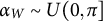
$\alpha _W \sim U(0, \pi ]$
,
$\{b_{Wj} \sim N(\mu _W, {\psi _W}^{-1}), j=1,\dots , J\}$
,
$\mu _W \sim N(0, 0.01^{-1}\psi _W)$
,
$\psi _W \sim \text {Gamma}(0.01, 0.01)$
; -
(iv) $\eta _R \sim U(-1, 1)$
,
$\alpha _R \sim U(0, \pi ]$
,
$\{b_{Rj} \sim N(\mu _R, {\psi _R}^{-1}), j=1,\dots , J-1\}$
,
$\mu _R \sim N(0, 0.01^{-1}\psi _R)$
,
$\psi _R \sim \text {Gamma}(0.01, 0.01)$
,














where
$(\mu _{Y}, \mu _T, \mu _W, \mu _R)'$
 and
$(\psi _{Y}, \psi _T, \psi _W, \psi _R)'$
and
$(\psi _{Y}, \psi _T, \psi _W, \psi _R)'$
 are the means and precisions of
$(\mathbf {{{b}}}_Y', {\mathbf {{{b}}}_T}', {\mathbf {{{b}}}_W}', {\mathbf {{{b}}}_R}')'$
are the means and precisions of
$(\mathbf {{{b}}}_Y', {\mathbf {{{b}}}_T}', {\mathbf {{{b}}}_W}', {\mathbf {{{b}}}_R}')'$
 . The joint posterior based on the observed data
$D_{\mathrm {obs}}$
. The joint posterior based on the observed data
$D_{\mathrm {obs}}$
 is written as

4.3 Bayesian model comparison—LPML decomposition
Similarly to the conventional LPML (Ibrahim, Chen, & Sinha, Reference Ibrahim, Chen and Sinha2001), we use the joint probability,
$\prod _{i=1}^n f(\mathbf {{{y}}}_i, \mathbf {{t}}_i, W_i, \mathbf {{{R}}}_i|\Omega )$
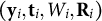
 , to measure the model’s predictive ability using a leave-one-out idea. Let
$D_{\mathrm {obs}}^{(-i)}=\{\mathbf {{{y}}}_{\ell , \mathrm {obs}}, \mathbf {{t}}_{\ell , \mathrm {obs}}, W_\ell , \mathbf {{{R}}}_\ell , \ell =1, \dots ,i-1, i+1, \dots , n\} $
, to measure the model’s predictive ability using a leave-one-out idea. Let
$D_{\mathrm {obs}}^{(-i)}=\{\mathbf {{{y}}}_{\ell , \mathrm {obs}}, \mathbf {{t}}_{\ell , \mathrm {obs}}, W_\ell , \mathbf {{{R}}}_\ell , \ell =1, \dots ,i-1, i+1, \dots , n\} $
 denote the observed data with
$(\mathbf {{{y}}}_i, \mathbf {{t}}_i, W_i, \mathbf {{{R}}}_i)$
denote the observed data with
$(\mathbf {{{y}}}_i, \mathbf {{t}}_i, W_i, \mathbf {{{R}}}_i)$
 deleted. Let
$D_{\mathbf {{W}} \mathbf {{{R}}}, \mathrm {obs}}^{(-i)}=\{W_\ell , \mathbf {{{R}}}_\ell , \ell =1, \dots ,i-1, i+1, \dots , n\} $
deleted. Let
$D_{\mathbf {{W}} \mathbf {{{R}}}, \mathrm {obs}}^{(-i)}=\{W_\ell , \mathbf {{{R}}}_\ell , \ell =1, \dots ,i-1, i+1, \dots , n\} $
 denote the observed data with
$(W_i, \mathbf {{{R}}}_i)$
denote the observed data with
$(W_i, \mathbf {{{R}}}_i)$
 deleted. Let
$\Omega _1$
deleted. Let
$\Omega _1$
 and
$\Omega _2$
and
$\Omega _2$
 denote the parameters of
$(\mathbf {{{y}}}, \mathbf {{t}})$
denote the parameters of
$(\mathbf {{{y}}}, \mathbf {{t}})$
 and
$(\mathbf {{W}}, \mathbf {{{R}}})$
and
$(\mathbf {{W}}, \mathbf {{{R}}})$
 , respectively. Specifically,
$\Omega _1=\{\mathbf {{{a}}}_Y, \mathbf {{{b}}}_Y, \mu _{Y},\psi _{Y}, {\mathbf {{{a}}}_T}, \mathbf {{{b}}}_{T}, \mu _T, \psi _T, \eta _T, \sigma _T \}$
, respectively. Specifically,
$\Omega _1=\{\mathbf {{{a}}}_Y, \mathbf {{{b}}}_Y, \mu _{Y},\psi _{Y}, {\mathbf {{{a}}}_T}, \mathbf {{{b}}}_{T}, \mu _T, \psi _T, \eta _T, \sigma _T \}$
 and
$\Omega _2=\{ \mathbf {{{b}}}_W, \mu _W,\psi _W, \eta _W,\alpha _W, \mathbf {{{b}}}_R, \mu _R,\psi _R, \eta _R, \alpha _R\}$
and
$\Omega _2=\{ \mathbf {{{b}}}_W, \mu _W,\psi _W, \eta _W,\alpha _W, \mathbf {{{b}}}_R, \mu _R,\psi _R, \eta _R, \alpha _R\}$
 .
.
The conditional predictive ordinate (CPO) identity (Geisser & Eddy, Reference Geisser and Eddy1979) for the i th subject is defined as

where
$\pi (\Omega |D_{\mathrm {obs}}^{(-i)})=\frac {\prod _{j \neq i} f(\mathbf {{{y}}}_i, \mathbf {{t}}_i, W_i, \mathbf {{{R}}}_i|\Omega )\pi (\Omega ) }{\int \prod _{j \neq i} f(\mathbf {{{y}}}_i, \mathbf {{t}}_i, W_i, \mathbf {{{R}}}_i|\Omega )\pi (\Omega ) d \Omega }$
 and LPML is defined as
$\text {LPML}=\sum _{i=1}^n\log \text {CPO}_{i}$
and LPML is defined as
$\text {LPML}=\sum _{i=1}^n\log \text {CPO}_{i}$
 ,
,
Using CPO identity III (Zhang et al., Reference Zhang, Chen, Ibrahim, Boye and Shen2017), we have

for any value of
$\Omega $
 . CPO
$_i$
. CPO
$_i$
 can be decomposed as

where

and

Proposition 4.1. The total LPML under the proposed joint model can be decomposed as

where
$\text {LPML}_{\mathbf {{{y}}}\mathbf {{t}}}=\sum _{i=1}^n\log \text {CPO}_{i, \mathbf {{{y}}}\mathbf {{t}}}$
 and
$\text {LPML}_{ \mathbf {{W}} \mathbf {{{R}}}|\mathbf {{{y}}}\mathbf {{t}}}=\sum _{i=1}^n \log \text {CPO}_{i, \mathbf {{W}} \mathbf {{{R}}}|\mathbf {{{y}}}\mathbf {{t}}}$
and
$\text {LPML}_{ \mathbf {{W}} \mathbf {{{R}}}|\mathbf {{{y}}}\mathbf {{t}}}=\sum _{i=1}^n \log \text {CPO}_{i, \mathbf {{W}} \mathbf {{{R}}}|\mathbf {{{y}}}\mathbf {{t}}}$
 .
.
To compute
$\text {LPML}_{ \mathbf {{W}} \mathbf {{{R}}}|\mathbf {{{y}}}\mathbf {{t}}}$
 , we start with Remark 4 of Zhang et al. (Reference Zhang, Chen, Ibrahim, Boye and Shen2017),

where we plug in a fixed value of
$\Omega _1$
 such as the posterior mean, denoted by
$\bar \Omega _1$
such as the posterior mean, denoted by
$\bar \Omega _1$
 .
.
Together with (15), we obtain

where
$\int k( \theta _{Yi}, \theta _{Wi},\theta _{Ri}| \bar \Omega _1, \Omega _2,\mathbf {{{y}}}_i,\mathbf {{t}}_i, W_i,\mathbf {{{R}}}_i ) d \theta _{Yi} d \theta _{Wi} d \theta _{Ri} =1$
 and
$\pi (\Omega _2, \theta _{Yi}, \theta _{Wi},\theta _{Ri}|\bar \Omega _1, D_{\mathrm {obs}})$
and
$\pi (\Omega _2, \theta _{Yi}, \theta _{Wi},\theta _{Ri}|\bar \Omega _1, D_{\mathrm {obs}})$
 is the conditional posterior density of
$(\Omega _2, \theta _{Yi}, \theta _{Wi},\theta _{Ri})$
is the conditional posterior density of
$(\Omega _2, \theta _{Yi}, \theta _{Wi},\theta _{Ri})$
 given
$\bar \Omega _1$
given
$\bar \Omega _1$
 and
$ D_{\mathrm {obs}}$
and
$ D_{\mathrm {obs}}$
 . In both simulations and real data analysis, we choose a multivariate normal distribution for
$k( \theta _{Yi}, \theta _{Wi},\theta _{Ri}| \bar \Omega _1, \Omega _2,\mathbf {{{y}}}_i,\mathbf {{t}}_i, W_i,\mathbf {{{R}}}_i ) $
. In both simulations and real data analysis, we choose a multivariate normal distribution for
$k( \theta _{Yi}, \theta _{Wi},\theta _{Ri}| \bar \Omega _1, \Omega _2,\mathbf {{{y}}}_i,\mathbf {{t}}_i, W_i,\mathbf {{{R}}}_i ) $
 that approximates
$f(\mathbf {{{y}}}_i | \theta _{Yi}, \bar \Omega _1) f(W_i, \mathbf {{{R}}}_i| \theta _{Wi},\theta _{Ri}, \Omega _2)f( \theta _{Yi}, \theta _{Wi}, \theta _{Ri}|\mathbf {{t}}_i)$
that approximates
$f(\mathbf {{{y}}}_i | \theta _{Yi}, \bar \Omega _1) f(W_i, \mathbf {{{R}}}_i| \theta _{Wi},\theta _{Ri}, \Omega _2)f( \theta _{Yi}, \theta _{Wi}, \theta _{Ri}|\mathbf {{t}}_i)$
 . The remaining two conditional densities that need to be computed are
$f(\mathbf {{{y}}}_i|\mathbf {{t}}_i,\bar \Omega _1) $
. The remaining two conditional densities that need to be computed are
$f(\mathbf {{{y}}}_i|\mathbf {{t}}_i,\bar \Omega _1) $
 and
$f( \theta _{Yi}, \theta _{Wi}, \theta _{Ri}|\mathbf {{t}}_i)$
and
$f( \theta _{Yi}, \theta _{Wi}, \theta _{Ri}|\mathbf {{t}}_i)$
 .
.
To compute
$f(\mathbf {{{y}}}_i|\mathbf {{t}}_i,\bar \Omega _1)$
 , we apply the formula:

where

and
$\theta _{Ti}| \theta _{Yi} \sim N(\sigma _{\theta \theta _T} \theta _{Yi}, 1-\sigma _{\theta \theta _T}^2)$
 . After some algebra, we obtain

Thus,

To determine
$f( \theta _{Yi}, \theta _{Wi}, \theta _{Ri}|\mathbf {{t}}_i)$
 , we apply the formula:

where
$\theta _{Ti}| \theta _{Yi}, \theta _{Wi}, \theta _{Ri} \sim N(\gamma _1\theta _{i}+\gamma _2\theta _{Wi}+\gamma _3\theta _{Ri}, \gamma _4)$
 ,
$(\gamma _1, \gamma _2, \gamma _3)'= \Sigma _{2, 134}'\Sigma _{134}^{-1}$
,
$(\gamma _1, \gamma _2, \gamma _3)'= \Sigma _{2, 134}'\Sigma _{134}^{-1}$
 ,
$\gamma _4=1-\Sigma _{2, 134}'\Sigma _{134}^{-1}\Sigma _{2, 134}$
,
$\gamma _4=1-\Sigma _{2, 134}'\Sigma _{134}^{-1}\Sigma _{2, 134}$
 ,
$\Sigma _{2, 134}=(\sigma _{\theta \theta _T}, \sigma _{\theta _T\theta _W}, \sigma _{\theta _T\theta _R})'$
,
$\Sigma _{2, 134}=(\sigma _{\theta \theta _T}, \sigma _{\theta _T\theta _W}, \sigma _{\theta _T\theta _R})'$
 , and
$\Sigma _{134}$
, and
$\Sigma _{134}$
 is the covariance matrix corresponding to
$ \theta _{Yi}$
is the covariance matrix corresponding to
$ \theta _{Yi}$
 ,
$\theta _{Wi}$
,
$\theta _{Wi}$
 , and
$\theta _{Ri}$
, and
$\theta _{Ri}$
 . After some algebra, we have

where
$ {{\boldsymbol {\mu }}}^*_i= -\frac {\bar {\sigma }_T \sum _{j=1}^{w_i-1}(1-r_{ij})\bar {a}_{Yj} (\log (t_{ij})-\bar {b}_{Tj})}{\bar {\sigma }_T^2\sum _{j=1}^{w_i-1}\bar {a}_{Yj}\gamma _4+1}\Sigma ^*_i \begin {bmatrix} \gamma _1\\ \gamma _2\\ \gamma _3 \end {bmatrix} $
 ,
,

$\kappa _{ikk'}=\frac {\bar {\sigma }_T^2 \sum _{j=1}^{w_i-1}(1-r_{ij})\bar {a}_{Yj} \gamma _k \gamma _{k'}}{\bar {\sigma }_T^2\sum _{j=1}^{w_i-1}\bar {a}_{Yj}\gamma _4+1}$
 , and
$\gamma _0=1-\sigma _{\theta \theta _W}^2-\sigma _{\theta \theta _R}^2-\sigma _{\theta _W\theta _R}^2+2\sigma _{\theta \theta _W}\sigma _{\theta \theta _R}\sigma _{\theta _W\theta _R}$
, and
$\gamma _0=1-\sigma _{\theta \theta _W}^2-\sigma _{\theta \theta _R}^2-\sigma _{\theta _W\theta _R}^2+2\sigma _{\theta \theta _W}\sigma _{\theta \theta _R}\sigma _{\theta _W\theta _R}$
 .
.
Similarly to a traditional LPML, a higher value of
$\text {LPML}_{\mathbf {{W}} \mathbf {{{R}}}|\mathbf {{{y}}} \mathbf {{t}}}$
 indicates a more favorable model in terms of prediction.
Remark 4.1. To measure the extent to which the missing data mechanism is nonignorable, we introduce
$\Delta \text {LPML}=\text {LPML}_{\mathbf {{W}}\mathbf {{{R}}}|\mathbf {{{y}}}\mathbf {{t}}} -\text {LPML}_{\mathbf {{W}}\mathbf {{{R}}}}$
 , where
$\text {LPML}_{\mathbf {{W}}\mathbf {{{R}}}}=\sum _{i=1}^n\log \text {CPO}_{i, \mathbf {{W}}\mathbf {{{R}}}}$
, where
$\text {LPML}_{\mathbf {{W}}\mathbf {{{R}}}}=\sum _{i=1}^n\log \text {CPO}_{i, \mathbf {{W}}\mathbf {{{R}}}}$
 and
$\text {CPO}_{i, \mathbf {{W}}\mathbf {{{R}}}}$
and
$\text {CPO}_{i, \mathbf {{W}}\mathbf {{{R}}}}$
 is calculated solely based on the joint model of
$\mathbf {{W}}$
is calculated solely based on the joint model of
$\mathbf {{W}}$
 and
$\mathbf {{{R}}}$
and
$\mathbf {{{R}}}$
 . Specifically,
$\Big [ \text {CPO}_{i, \mathbf {{W}} \mathbf {{{R}}}} \Big ]^{-1} = \int \frac {k( \theta _{Wi},\theta _{Ri}| \Omega _2, W_i,\mathbf {{{R}}}_i )\pi (\Omega _2, \theta _{Wi},\theta _{Ri}|D_{\mathrm {obs}})}{ f(W_i, \mathbf {{{R}}}_i| \theta _{Wi},\theta _{Ri}, \Omega _2)f( \theta _{Wi}, \theta _{Ri}) } d\theta _W d\theta _Rd\Omega _2,$
. Specifically,
$\Big [ \text {CPO}_{i, \mathbf {{W}} \mathbf {{{R}}}} \Big ]^{-1} = \int \frac {k( \theta _{Wi},\theta _{Ri}| \Omega _2, W_i,\mathbf {{{R}}}_i )\pi (\Omega _2, \theta _{Wi},\theta _{Ri}|D_{\mathrm {obs}})}{ f(W_i, \mathbf {{{R}}}_i| \theta _{Wi},\theta _{Ri}, \Omega _2)f( \theta _{Wi}, \theta _{Ri}) } d\theta _W d\theta _Rd\Omega _2,$
 where
$k(\theta _{Wi},\theta _{Ri}| \Omega _2, W_i,\mathbf {{{R}}}_i )$
where
$k(\theta _{Wi},\theta _{Ri}| \Omega _2, W_i,\mathbf {{{R}}}_i )$
 is a bivariate normal distribution that approximates the joint posterior distribution of
$\Omega _2$
is a bivariate normal distribution that approximates the joint posterior distribution of
$\Omega _2$
 .
.
$\text {LPML}_{\mathbf {{W}}\mathbf {{{R}}}|\mathbf {{{y}}} \mathbf {{t}}}$
 is reduced to
$\text {LPML}_{\mathbf {{W}}\mathbf {{{R}}}}$
is reduced to
$\text {LPML}_{\mathbf {{W}}\mathbf {{{R}}}}$
 and consequently
$\Delta \text {LPML}$
and consequently
$\Delta \text {LPML}$
 is
$0$
is
$0$
 if the missing data mechanism is ignorable, that is,
$\eta _W=\eta _R=0$
if the missing data mechanism is ignorable, that is,
$\eta _W=\eta _R=0$
 . This formulation, by integrating the latent variables associated with
$\mathbf {{t}}$
. This formulation, by integrating the latent variables associated with
$\mathbf {{t}}$
 , enables the evaluation of multidimensional integrals, making it computationally efficient. Furthermore, it simplifies the comparison between the joint model of (
$\mathbf {{{y}}}, \mathbf {{t}}$
, enables the evaluation of multidimensional integrals, making it computationally efficient. Furthermore, it simplifies the comparison between the joint model of (
$\mathbf {{{y}}}, \mathbf {{t}}$
 ) and the single outcome model of
$\mathbf {{{y}}}$
) and the single outcome model of
$\mathbf {{{y}}}$
 , as
$\text {CPO}_{i, \mathbf {{W}} \mathbf {{{R}}}|\mathbf {{{y}}}\mathbf {{t}}}$
, as
$\text {CPO}_{i, \mathbf {{W}} \mathbf {{{R}}}|\mathbf {{{y}}}\mathbf {{t}}}$
 and
$\text {CPO}_{i, \mathbf {{W}} \mathbf {{{R}}}|\mathbf {{{y}}}}$
and
$\text {CPO}_{i, \mathbf {{W}} \mathbf {{{R}}}|\mathbf {{{y}}}}$
 share the same dimension.
Remark 4.2. To assess the importance of modeling item response (
$\mathbf {{{y}}}$
 ) and response time (
$\mathbf {{t}}$
) and response time (
$\mathbf {{t}}$
 ) jointly versus individually (
$\mathbf {{{y}}}-$
) jointly versus individually (
$\mathbf {{{y}}}-$
 only or
$\mathbf {{t}}-$
only or
$\mathbf {{t}}-$
 only) in identifying the missing data mechanism, we consider the following single response models. The first single response model we compare is the one that includes only
$\mathbf {{{y}}}$
only) in identifying the missing data mechanism, we consider the following single response models. The first single response model we compare is the one that includes only
$\mathbf {{{y}}}$
 , where (11) is reformulated as follows:

Consequently,

where
$\int k( \theta _{Yi}, \theta _{Wi},\theta _{Ri}| \bar \Omega _1, \Omega _2,\mathbf {{{y}}}_i,W_i,\mathbf {{{R}}}_i ) d \theta _{Yi} d \theta _{Wi} d \theta _{Ri} =1$
 . The second single response model we compare is the one that includes only
$\mathbf {{t}}$
. The second single response model we compare is the one that includes only
$\mathbf {{t}}$
 , where (11) is reformulated as follows:

Consequently,

where
$\int k( \theta _{Yi}, \theta _{Wi},\theta _{Ri}| \bar \Omega _1, \Omega _2,\mathbf {{t}}_i,W_i,\mathbf {{{R}}}_i ) d \theta _{Ti} d \theta _{Wi} d \theta _{Ri} =1$
 .
.
We then compute
$\text {LPML}_{\mathbf {{W}}\mathbf {{{R}}}|\mathbf {{{y}}} \mathbf {{t}}}$
 -
$\text {LPML}_{\mathbf {{W}}\mathbf {{{R}}}|\mathbf {{{y}}}}$
-
$\text {LPML}_{\mathbf {{W}}\mathbf {{{R}}}|\mathbf {{{y}}}}$
 and
$\text {LPML}_{\mathbf {{W}}\mathbf {{{R}}}|\mathbf {{{y}}} \mathbf {{t}}}$
and
$\text {LPML}_{\mathbf {{W}}\mathbf {{{R}}}|\mathbf {{{y}}} \mathbf {{t}}}$
 -
$\text {LPML}_{\mathbf {{W}}\mathbf {{{R}}}|\mathbf {{t}}}$
-
$\text {LPML}_{\mathbf {{W}}\mathbf {{{R}}}|\mathbf {{t}}}$
 , respectively. A positive value indicates that the joint model provides a better fit for the missing data model. We can also compare between
$\text {LPML}_{\mathbf {{W}}\mathbf {{{R}}}|\mathbf {{{y}}}}$
, respectively. A positive value indicates that the joint model provides a better fit for the missing data model. We can also compare between
$\text {LPML}_{\mathbf {{W}}\mathbf {{{R}}}|\mathbf {{{y}}}}$
 and
$\text {LPML}_{\mathbf {{W}}\mathbf {{{R}}}|\mathbf {{t}}}$
and
$\text {LPML}_{\mathbf {{W}}\mathbf {{{R}}}|\mathbf {{t}}}$
 , where a larger value indicates that the corresponding outcome model provides better identification of the missing data mechanism.
5 Simulations
In this section, we conduct extensive simulation studies to examine the performance of
$\text {LPML}_{\mathbf {{W}} \mathbf {{{R}}}|\mathbf {{{y}}} \mathbf {{t}}}$
 on model selection and the performance of the proposed nonignorable and ignorable missing data mechanisms in modeling the simulated missing data. In all Bayesian computations, we use 5,000 MCMC samples, which are taken from every tenth iteration, after a burn-in of 5,000 iterations for each model to compute all the posterior estimates, including posterior means, posterior standard deviations, 95% highest posterior density (HPD) intervals, and
$\text {LPML}_{\mathbf {{W}} \mathbf {{{R}}}|\mathbf {{{y}}} \mathbf {{t}}}$
on model selection and the performance of the proposed nonignorable and ignorable missing data mechanisms in modeling the simulated missing data. In all Bayesian computations, we use 5,000 MCMC samples, which are taken from every tenth iteration, after a burn-in of 5,000 iterations for each model to compute all the posterior estimates, including posterior means, posterior standard deviations, 95% highest posterior density (HPD) intervals, and
$\text {LPML}_{\mathbf {{W}} \mathbf {{{R}}}|\mathbf {{{y}}} \mathbf {{t}}}$
 . The MCMC sampling code is written with R package nimble (de Valpine et al., Reference de Valpine, Turek, Paciorek, Anderson-Bergman, Temple Lang and Bodik2017) with double-precision accuracy. The code for computing the
$\text {LPML}_{\mathbf {{W}} \mathbf {{{R}}}|\mathbf {{{y}}} \mathbf {{t}}}$
. The MCMC sampling code is written with R package nimble (de Valpine et al., Reference de Valpine, Turek, Paciorek, Anderson-Bergman, Temple Lang and Bodik2017) with double-precision accuracy. The code for computing the
$\text {LPML}_{\mathbf {{W}} \mathbf {{{R}}}|\mathbf {{{y}}} \mathbf {{t}}}$
 is written in FORTRAN 95 using IMSL subroutines with double-precision accuracy. The convergence of the MCMC samples is checked by the R package “mcmcplots” using R version 4.5.2. Convergence is reached approximately after 5,000 iterations. The codes for nimble and Fortran are provided in the Supplementary Material.
5.1 Simulation Scenarios I and II
The purpose of simulations in this section is to investigate the impact of misspecification of the missing data model under a setting similar to that of the real data. In Simulation Scenarios I and II, we first generate
$S = 1,000$
 replications. For each replication, we set the total number of subjects (n) equal to
$2,000$
replications. For each replication, we set the total number of subjects (n) equal to
$2,000$
 and the total number of items (J) equal to
$12$
and the total number of items (J) equal to
$12$
 to mimic the real data. The binary responses
$y_{ij}$
to mimic the real data. The binary responses
$y_{ij}$
 are generated based on the item response model in (1), where the
$a_{Yj}$
are generated based on the item response model in (1), where the
$a_{Yj}$
 s are sampled from a truncated normal distribution with a lower bound of 0.2 and an upper bound of 1,
$b_{Yj} \sim N(\mu _{Y}, \psi _{Y}^{-1})$
s are sampled from a truncated normal distribution with a lower bound of 0.2 and an upper bound of 1,
$b_{Yj} \sim N(\mu _{Y}, \psi _{Y}^{-1})$
 with
$\mu _{Y} = 1$
with
$\mu _{Y} = 1$
 and
$\psi _{Y} = 1$
and
$\psi _{Y} = 1$
 for
$j = 1, \dots , J$
for
$j = 1, \dots , J$
 . The response times
$t_{ij}$
. The response times
$t_{ij}$
 are generated based on the model in (2), where
$a_{Tj}$
are generated based on the model in (2), where
$a_{Tj}$
 s are sampled from a truncated normal distribution with a lower bound of 0.5 and an upper bound of 4,
$\eta _T=-0.4$
s are sampled from a truncated normal distribution with a lower bound of 0.5 and an upper bound of 4,
$\eta _T=-0.4$
 ,
$b_{Tj} \sim N(\mu _T, \psi _T^{-1})$
,
$b_{Tj} \sim N(\mu _T, \psi _T^{-1})$
 with
$\mu _T = 2$
with
$\mu _T = 2$
 and
$\psi _T = 1$
and
$\psi _T = 1$
 for
$j = 1, \dots , J$
for
$j = 1, \dots , J$
 . For the missing data models in Simulation Scenarios I and II, the not-reached items
$W_i$
. For the missing data models in Simulation Scenarios I and II, the not-reached items
$W_i$
 are generated based on models in (3)–(5), where
$b_{Wj} \sim N(\mu _W, \psi _W^{-1})$
are generated based on models in (3)–(5), where
$b_{Wj} \sim N(\mu _W, \psi _W^{-1})$
 with
$\mu _W = 6$
with
$\mu _W = 6$
 and
$\psi _W = 1$
and
$\psi _W = 1$
 for
$j = 1, \dots , J$
for
$j = 1, \dots , J$
 , to mimic the real data. The omitted items,
$R_{i\ell }$
, to mimic the real data. The omitted items,
$R_{i\ell }$
 s, are generated based on models in (6) and (7), where
$b_{Rj} \sim N(\mu _R, \psi _R^{-1})$
s, are generated based on models in (6) and (7), where
$b_{Rj} \sim N(\mu _R, \psi _R^{-1})$
 with
$\mu _R = 2$
with
$\mu _R = 2$
 and
$\psi _R = 1$
and
$\psi _R = 1$
 for
$j = 1, \dots , J$
for
$j = 1, \dots , J$
 . To investigate the associations between the latent propensity parameters, we independently generate
$ \theta _{Yi}, \zeta _{Ti}, \zeta _{Wi}, \zeta _{Ri} \sim N(0, 1)$
. To investigate the associations between the latent propensity parameters, we independently generate
$ \theta _{Yi}, \zeta _{Ti}, \zeta _{Wi}, \zeta _{Ri} \sim N(0, 1)$
 for each replication,
$i=1, \dots , n$
for each replication,
$i=1, \dots , n$
 .
.
The only differences between Simulation Scenarios I and II are the choices of
$\eta _W$
 ,
$\alpha _W$
,
$\alpha _W$
 ,
$\eta _R$
,
$\eta _R$
 , and
$\alpha _R$
, and
$\alpha _R$
 . In Simulation Scenario I, we set
$\eta _W = -0.3$
. In Simulation Scenario I, we set
$\eta _W = -0.3$
 ,
$\alpha _W = 1.3$
,
$\alpha _W = 1.3$
 ,
$\eta _{R} = -0.5$
,
$\eta _{R} = -0.5$
 , and
$\alpha _R = 1.7$
, and
$\alpha _R = 1.7$
 to mimic the real data in Section 6. In Simulation Scenario II, all values are set to 0 to generate an ignorable missing data mechanism. In both settings, the missing data percentages of the simulated datasets are around 20%, with 15% due to omission behavior and 5% due to not-reached behavior, which is similar to the real data. The missing percentages by item are provided in Figures S1 and S2 in the Supplementary Material.
We fit both nonignorable and ignorable models to the simulated nonignorable datasets in Simulation Scenario I and the simulated ignorable datasets in Simulation Scenario II. The boxplots of the differences values
$\Delta \text {LPML}_{\mathbf {{W}} \mathbf {{{R}}}|\mathbf {{{y}}} \mathbf {{t}}}$
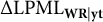 (Nonignorable–Ignorable) under these two models are given in Figure 2. For Simulation Scenario I where the true missing data mechanism is nonignorable, the median of the values of
$\text {LPML}_{\mathbf {W} \mathbf {R}|\mathbf {y} \mathbf {t}}$
(Nonignorable–Ignorable) under these two models are given in Figure 2. For Simulation Scenario I where the true missing data mechanism is nonignorable, the median of the values of
$\text {LPML}_{\mathbf {W} \mathbf {R}|\mathbf {y} \mathbf {t}}$
 under the nonignorable model (
$-$
under the nonignorable model (
$-$
 9674.02) is greater than that under the ignorable model (
$-$
9674.02) is greater than that under the ignorable model (
$-$
 9738.74). Furthermore, the entire boxplot (Median=63.86, IQR=(55.90, 72.34)) for
$\Delta \text {LPML}_{\mathbf {W} \mathbf {R}|\mathbf {y} \mathbf {t}}$
9738.74). Furthermore, the entire boxplot (Median=63.86, IQR=(55.90, 72.34)) for
$\Delta \text {LPML}_{\mathbf {W} \mathbf {R}|\mathbf {y} \mathbf {t}}$
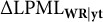 is above 0 (Figure 2 left panel in red), indicating that
$\text {LPML}_{\mathbf {W} \mathbf {R}|\mathbf {y} \mathbf {t}}$
is above 0 (Figure 2 left panel in red), indicating that
$\text {LPML}_{\mathbf {W} \mathbf {R}|\mathbf {y} \mathbf {t}}$
 correctly selects the best model in this case. For Simulation Scenario II where the true missing data mechanism is ignorable, the median of the values of
$\text {LPML}_{\mathbf {W} \mathbf {R}|\mathbf {y} \mathbf {t}}$
correctly selects the best model in this case. For Simulation Scenario II where the true missing data mechanism is ignorable, the median of the values of
$\text {LPML}_{\mathbf {W} \mathbf {R}|\mathbf {y} \mathbf {t}}$
 under the ignorable model (
$-$
under the ignorable model (
$-$
 9240.21) is slightly greater than that under the nonignorable model (
$-$
9240.21) is slightly greater than that under the nonignorable model (
$-$
 9241.49). The horizontal
$y=0$
9241.49). The horizontal
$y=0$
 line intersects the whisker of the boxplot (Median=
$-$
line intersects the whisker of the boxplot (Median=
$-$
 1.18, IQR=(
$-$
1.18, IQR=(
$-$
 1.79,
$-$
1.79,
$-$
 0.29)). This is expected as the nonignorable model is approximately ignorable when the estimates of
$\eta _T, \eta _W$
0.29)). This is expected as the nonignorable model is approximately ignorable when the estimates of
$\eta _T, \eta _W$
 , and
$\eta _R$
, and
$\eta _R$
 are close to zero, as observed in Scenario II. However, the
$\Delta \text {LPML}_{\mathbf {{W}} \mathbf {{{R}}}|\mathbf {{{y}}} \mathbf {{t}}}$
are close to zero, as observed in Scenario II. However, the
$\Delta \text {LPML}_{\mathbf {{W}} \mathbf {{{R}}}|\mathbf {{{y}}} \mathbf {{t}}}$
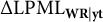 measure accounts for the dimension penalty, as reflected in the boxplot. The entire box for
$\Delta \text {LPML}_{\mathbf {{W}} \mathbf {{{R}}}|\mathbf {{{y}}} \mathbf {{t}}}$
measure accounts for the dimension penalty, as reflected in the boxplot. The entire box for
$\Delta \text {LPML}_{\mathbf {{W}} \mathbf {{{R}}}|\mathbf {{{y}}} \mathbf {{t}}}$
 is below 0 (Figure 2 right panel in cyan), indicating that
$\text {LPML}_{\mathbf {{W}} \mathbf {{{R}}}|\mathbf {{{y}}} \mathbf {{t}}}$
is below 0 (Figure 2 right panel in cyan), indicating that
$\text {LPML}_{\mathbf {{W}} \mathbf {{{R}}}|\mathbf {{{y}}} \mathbf {{t}}}$
 effectively selects the true model in this case. In conclusion,
$\text {LPML}_{\mathbf {{W}} \mathbf {{{R}}}|\mathbf {{{y}}} \mathbf {{t}}}$
effectively selects the true model in this case. In conclusion,
$\text {LPML}_{\mathbf {{W}} \mathbf {{{R}}}|\mathbf {{{y}}} \mathbf {{t}}}$
 can serve as a good criterion for selecting a better model in these two different settings.
Boxplots of
$\Delta \text {LPML}_{\mathbf {{W}} \mathbf {{{R}}}|\mathbf {{{y}}} \mathbf {{t}}}$
 (Nonignorable–Ignorable) when the true missing data mechanisms are nonignorable (Simulation Scenario I in red) and ignorable (Simulation Scenario II in cyan).

In Tables 1 and 2, we report the differences between the posterior mean and the true value (Bias), the standard deviation of the estimate (SD), the root mean squared error of the posterior mean (RMSE), and the coverage probability (CP) of the 95% HPD interval for each parameter in the item response, response time, and missing data models under the optimal models in Simulations I (i.e., nonignorable) and II (i.e., ignorable), respectively. In both tables, the Bias and SDs of the posterior estimates are relatively small, SDs are similar to RMSEs, and most of the CPs are around the 95% nominal level. The CP for
$b_{Y7}$
 in Simulation Scenario I, which corresponds to the item with the smallest value of
$\mathbf {{{b}}}_Y$
in Simulation Scenario I, which corresponds to the item with the smallest value of
$\mathbf {{{b}}}_Y$
 and the highest missing percentage (median=58.50%), is slightly lower than the nominal level. Similarly, the CP for
$b_{Y4}$
and the highest missing percentage (median=58.50%), is slightly lower than the nominal level. Similarly, the CP for
$b_{Y4}$
 and
$b_{W11}$
and
$b_{W11}$
 in Simulation Scenario II, which correspond to the item with the largest value of
$\mathbf {{{b}}}_Y$
in Simulation Scenario II, which correspond to the item with the largest value of
$\mathbf {{{b}}}_Y$
 and the highest missing percentage (median=57.45%), and the item with the largest value of
$\mathbf {{{b}}}_W$
and the highest missing percentage (median=57.45%), and the item with the largest value of
$\mathbf {{{b}}}_W$
 and the second highest missing percentage (median=48.20%), respectively, are slightly lower than the nominal level. These CPs are improved when sample size increases, as shown in Simulation Scenario VIII.
Bias, SD, RMSE, and CP of parameters in the item response model, the response time model, and the missing data models under the nonignorable missing data mechanism in Simulation Scenario I (
$n=2,000$
 ,
$J=12$
,
$J=12$
 , median sizes of
$\eta $
, median sizes of
$\eta $
 s, 20% missing data percentage (15% due to omission + 5% due to not-reached), and the true missing data mechanism is nonignorable)

Table 1 Long description
The table is organized into two main vertical sections, each containing columns for Parameter, Bias, S D, R M S E, and C P.
* The first section includes parameters a sub Y 1 through a sub Y 12, a sub T 1 through a sub T 12, and b sub W 1 through b sub W 12. It also includes eta sub T, eta sub W, alpha sub W, eta sub R, and alpha sub R.
* The second section includes parameters b sub Y 1 through b sub Y 12, b sub T 1 through b sub T 12, b sub W 1 through b sub W 12, b sub R 1 through b sub R 11, and sigma sub T.
Key data points include:
* For a sub Y 1: Bias is minus 0.012, S D is 0.092, R M S E is 0.096, and C P is 0.942.
* For b sub Y 1: Bias is 0.026, S D is 0.114, R M S E is 0.119, and C P is 0.930.
* For a sub T 1: Bias is 0.010, S D is 0.104, R M S E is 0.109, and C P is 0.933.
* For b sub T 1: Bias is 0.001, S D is 0.019, R M S E is 0.019, and C P is 0.952.
* For b sub W 1: Bias is minus 0.011, S D is 0.541, R M S E is 0.516, and C P is 0.959.
* For b sub R 1: Bias is 0.004, S D is 0.059, R M S E is 0.059, and C P is 0.943.
* For sigma sub T: Bias is 0.000, S D is 0.008, R M S E is 0.008, and C P is 0.940.
* For alpha sub R: Bias is 0.010, S D is 0.091, R M S E is 0.090, and C P is 0.952.
Bias, SD, RMSE, and CP of parameters in the item response model, the response time model, and the missing data models under the ignorable missing data mechanism in Simulation Scenario II (
$n=2,000$
 ,
$J=12$
,
$J=12$
 ,
$\eta _W=\eta _R=0$
,
$\eta _W=\eta _R=0$
 , 20% missing data percentage (15% due to omission + 5% due to not-reached), and the true missing data mechanism is ignorable)

Table 2 Long description
The table presents results for Simulation Scenario I I with n equals two thousand, J equals twelve, and twenty percent missing data (fifteen percent omission, five percent not-reached), under an ignorable missing data mechanism. Each row lists two parameters side by side, each with bias, standard deviation, root mean square error, and coverage probability. For item response model parameters a sub Y1 to a sub Y12, bias ranges from negative zero point zero zero four to zero point zero seven eight, standard deviation from zero point zero seven to zero point two zero six, root mean square error from zero point zero seven one to zero point two two three, and coverage probability from zero point nine three three to zero point nine five five. For corresponding b sub Y1 to b sub Y12, bias ranges from negative zero point zero one seven to zero point zero three six, standard deviation from zero point zero six five to zero point one seven eight, root mean square error from zero point zero six seven to zero point one seventy two, and coverage probability from zero point nine three two to zero point nine six three. Response time model parameters a sub T10 to a sub T12 and b sub T10 to b sub T12 show bias between zero and zero point zero four, standard deviation from zero point zero eight two to zero point one zero one, root mean square error from zero point zero eight two to zero point one zero one, and coverage probability from zero point nine three four to zero point nine five two. For missing data models, parameters b sub W10 to b sub W12, b sub R10 to b sub R12, and sigma sub T, bias ranges from negative zero point seven eight one to zero point zero six, standard deviation from zero point zero zero eight to zero point seven two three, root mean square error from zero point zero zero eight to zero point eight seven six, and coverage probability from zero point eight four one to zero point nine five seven. Notably, b sub W11 shows the largest negative bias at negative zero point seven eight one and lowest coverage probability at zero point eight four one, while sigma sub T has the smallest bias and standard deviation. The table allows direct comparison of estimation accuracy and reliability across all parameters and models.
To further investigate the performance of the
$ {\theta }$
 estimates, we conduct an additional simulation under the same setting as Simulation Scenario I, except that
$ {\theta }$
estimates, we conduct an additional simulation under the same setting as Simulation Scenario I, except that
$ {\theta }$
 is fixed across repetitions. The posterior summaries of
${\theta }$
is fixed across repetitions. The posterior summaries of
${\theta }$
 also exhibit good performance, with the following median (IQR) values: bias=
$-$
also exhibit good performance, with the following median (IQR) values: bias=
$-$
 0.058 (
$-$
0.058 (
$-$
 0.363,
$-$
0.363,
$-$
 0.021), SD=0.701 (0.688, 0.704), RMSE=0.606 (0.523, 0.681), and CP=0.976 (0.940, 0.989).
Under the same setting of Simulation Scenario I, we compare our methods with multivariate imputation by chained equations (MICE) methods (Rubin, Reference Rubin1987; Van Buuren & Groothuis-Oudshoorn, Reference Van Buuren and Groothuis-Oudshoorn2011) in Table 3. Twenty mutiple imputations are performed. The same item response and response time models in (1) and (2) and the same hierarchical framework and reparameterization techniques in Section 3 are assumed for fair comparison. Weighted predicted mean matching method is used for the imputation step. The posterior summaries of the response models are good, while poor CPs are observed for the parameters in the response time model. The two missing data behaviors are not studied under MICE and the method is computationally intensive.
Bias, SD, RMSE, and CP of parameters in the item response model and the response time model under MICE in Simulation Scenario I (
$n=2,000$
 ,
$J=12$
,
$J=12$
 , median sizes of
$\eta $
, median sizes of
$\eta $
 s, 20% missing data percentage (15% due to omission + 5% due to not-reached), and the true missing data mechanism is nonignorable)

Table 3 Long description
Starting from the top row, the table lists parameters for item response and response time models in pairs. Each parameter is followed by four columns: Bias, S D, R M S E, and C P. For example, a sub Y 1 has Bias negative 0.022, S D 0.094, R M S E 0.100, C P 0.932; b sub Y 1 has Bias negative 0.037, S D 0.117, R M S E 0.126, C P 0.911. This pattern continues for all item parameters from a sub Y 1 to a sub Y 12 and b sub Y 1 to b sub Y 12, as well as for time parameters a sub T 10 to a sub T 12 and b sub T 10 to b sub T 12. Additional parameters include sigma sub T with Bias 0.010, S D 0.008, R M S E 0.016, C P 0.783, and eta sub T with Bias 0.009, S D 0.038, R M S E 0.039, C P 0.937. Values for Bias are mostly close to zero, S D and R M S E vary across parameters, and C P values are generally above 0.9 except for sigma sub T. The table structure allows direct comparison of estimation accuracy and coverage probability for each parameter under the specified simulation conditions.
We also compare our methods with the RTprocess model (Lu & Wang, Reference Lu and Wang2020) in Table 4, where the item omission behavior is modeled as a type of censoring based on the response time model. Most of the posterior summaries of the response models are good, while large biases and poor CPs are observed for the parameters in the response time model and the correlation parameter
$\eta _T$
 . This is expected as the method assumes the omission and not-reached behaviors are solely due to time limitations. However, it does not account for the propensities of omission and not-reach that are incorporated in the simulation design. Additionally, we compare these three methods when data are generated from the RTprocess model, with a similar percentage of missingness (15% due to omission behavior and 5% due to not-reached behavior). Posterior summaries under the RTprocess model (Table S1 in the Supplementary Material) are good, as expected, since this is the data-generating model. Under the proposed nonignorable model, posterior summaries of most parameters (Table S2 in the Supplementary Material) are also satisfactory, except for several item-specific parameters in the response time model that correspond to high missingness, as well as
$\sigma _T$
. This is expected as the method assumes the omission and not-reached behaviors are solely due to time limitations. However, it does not account for the propensities of omission and not-reach that are incorporated in the simulation design. Additionally, we compare these three methods when data are generated from the RTprocess model, with a similar percentage of missingness (15% due to omission behavior and 5% due to not-reached behavior). Posterior summaries under the RTprocess model (Table S1 in the Supplementary Material) are good, as expected, since this is the data-generating model. Under the proposed nonignorable model, posterior summaries of most parameters (Table S2 in the Supplementary Material) are also satisfactory, except for several item-specific parameters in the response time model that correspond to high missingness, as well as
$\sigma _T$
 and
$\eta _T$
and
$\eta _T$
 . Results under MICE are the worst under this setting (see Table S3 in the Supplementary Material).
Bias, SD, RMSE, and CP of parameters in the item response model and the response time model under the response time process model in Simulation Scenario I (
$n=2,000$
 ,
$J=12$
,
$J=12$
 , median sizes of
$\eta $
, median sizes of
$\eta $
 s, 20% missing data percentage (15% due to omission + 5% due to not-reached), and the true missing data mechanism is nonignorable)

Table 4 Long description
Starting from the top row, the table displays two sets of columns for each parameter: item response model (left) and response time model (right). Each set includes Parameter, Bias, S D, R M S E, and C P. Parameters are labeled as a sub Y 1 through a sub Y 12 and b sub Y 1 through b sub Y 12 for the item response model, and a sub T 10 through a sub T 12 and b sub T 10 through b sub T 12 for the response time model. Bias values range from negative to positive, with most item response parameters showing low Bias (e.g., a sub Y 1 is negative 0.022), S D values between 0.071 and 0.123, R M S E values between 0.065 and 0.119, and C P values mostly above 0.9. Response time parameters display higher Bias (e.g., a sub T 10 is 0.179), S D values from 0.017 to 0.098, R M S E values from 0.019 to 0.200, and C P values varying from 0.000 to 0.942. Additional parameters include sigma sub T and eta sub T, with sigma sub T showing Bias 0.073, S D 0.038, R M S E 0.083, and C P 0.489, and eta sub T showing Bias negative 0.008, S D 0.008, R M S E 0.011, and C P 0.850. The table highlights that item response model parameters generally have higher coverage probabilities and lower error metrics compared to response time model parameters under the specified simulation scenario.
5.2 Simulation Scenarios III and IV
The purpose of simulations in this section is to investigate the impact of misspecification of the missing data model when the missing data percentages (30%) are higher than those in Scenarios I and II, with 20% due to omission behavior and 10% due to not-reached behavior. In Simulation Scenarios III and IV, we set
$\mu _W=5.5, \mu _R=1.5$
 to increase the missing data percentage while keeping all other conditions the same as in Scenarios I and II.
Similarly, we fit both nonignorable and ignorable models to the simulated nonignorable datasets in Simulation Scenario III and the simulated ignorable datasets in Simulation Scenario IV. The boxplots of the differences values
$\text {LPML}_{\mathbf {{W}} \mathbf {{{R}}}|\mathbf {{{y}}} \mathbf {{t}}}$
 (Nonignorable–Ignorable) under these two models are given in Figure 3. For Simulation Scenario III where the true missing data mechanism is nonignorable, the median of the values of
$\text {LPML}_{\mathbf {{W}} \mathbf {{{R}}}|\mathbf {{{y}}} \mathbf {{t}}}$
(Nonignorable–Ignorable) under these two models are given in Figure 3. For Simulation Scenario III where the true missing data mechanism is nonignorable, the median of the values of
$\text {LPML}_{\mathbf {{W}} \mathbf {{{R}}}|\mathbf {{{y}}} \mathbf {{t}}}$
 under the nonignorable model (
$-$
under the nonignorable model (
$-$
 11042.51) is greater than that under the ignorable model (
$-$
11042.51) is greater than that under the ignorable model (
$-$
 11106.94). Additionally, the box (Median=66.46, IQR=(58.64, 74.11)) for the
$\Delta \text {LPML}_{\mathbf {{W}} \mathbf {{{R}}}|\mathbf {{{y}}} \mathbf {{t}}}$
11106.94). Additionally, the box (Median=66.46, IQR=(58.64, 74.11)) for the
$\Delta \text {LPML}_{\mathbf {{W}} \mathbf {{{R}}}|\mathbf {{{y}}} \mathbf {{t}}}$
 is above 0 (Figure 3 left panel in red), indicating that the nonignorable model outperforms the ignorable model when the true missing data mechanism is nonignorable. For Simulation Scenario IV where the true missing data mechanism is ignorable, the median of the values of
$\text {LPML}_{\mathbf {{W}} \mathbf {{{R}}}|\mathbf {{{y}}} \mathbf {{t}}}$
is above 0 (Figure 3 left panel in red), indicating that the nonignorable model outperforms the ignorable model when the true missing data mechanism is nonignorable. For Simulation Scenario IV where the true missing data mechanism is ignorable, the median of the values of
$\text {LPML}_{\mathbf {{W}} \mathbf {{{R}}}|\mathbf {{{y}}} \mathbf {{t}}}$
 under the ignorable model (
$-$
under the ignorable model (
$-$
 10452.53) is slightly greater than that under the nonignorable model (
$-$
10452.53) is slightly greater than that under the nonignorable model (
$-$
 10453.09). Posterior estimates of
$\eta _T, \eta _W, $
10453.09). Posterior estimates of
$\eta _T, \eta _W, $
 and
$\eta _R$
and
$\eta _R$
 under the nonignorable model are close to 0, making it similar to the ignorable model. A key advantage of
$\text {LPML}_{\mathbf {{W}} \mathbf {{{R}}}|\mathbf {{{y}}} \mathbf {{t}}}$
under the nonignorable model are close to 0, making it similar to the ignorable model. A key advantage of
$\text {LPML}_{\mathbf {{W}} \mathbf {{{R}}}|\mathbf {{{y}}} \mathbf {{t}}}$
 is that it accounts for dimension penalty. The entire box (Median=
$-$
is that it accounts for dimension penalty. The entire box (Median=
$-$
 1.16, IQR=(
$-$
1.16, IQR=(
$-$
 1.87,
$-$
1.87,
$-$
 0.31)) for the
$\Delta \text {LPML}_{\mathbf {{W}} \mathbf {{{R}}}|\mathbf {{{y}}} \mathbf {{t}}}$
0.31)) for the
$\Delta \text {LPML}_{\mathbf {{W}} \mathbf {{{R}}}|\mathbf {{{y}}} \mathbf {{t}}}$
 is below 0 (Figure 3 right panel in cyan), indicating that the
$\text {LPML}_{\mathbf {{W}} \mathbf {{{R}}}|\mathbf {{{y}}} \mathbf {{t}}}$
is below 0 (Figure 3 right panel in cyan), indicating that the
$\text {LPML}_{\mathbf {{W}} \mathbf {{{R}}}|\mathbf {{{y}}} \mathbf {{t}}}$
 effectively selects the true model in this case. In conclusion, the
$\text {LPML}_{\mathbf {{W}} \mathbf {{{R}}}|\mathbf {{{y}}} \mathbf {{t}}}$
effectively selects the true model in this case. In conclusion, the
$\text {LPML}_{\mathbf {{W}} \mathbf {{{R}}}|\mathbf {{{y}}} \mathbf {{t}}}$
 can serve as a good criterion for selecting a better model under these two different settings.
Boxplots of
$\Delta \text {LPML}_{\mathbf {{W}} \mathbf {{{R}}}|\mathbf {{{y}}} \mathbf {{t}}}$
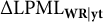 (Nonignorable–Ignorable) when the true missing data mechanisms are nonignorable (Simulation Scenario III in red) and ignorable (Simulation Scenario IV in cyan).

Figure 3 Long description
The left panel labeled Scenario III displays a red boxplot with a median near 62, interquartile range from about 50 to 70, and several outliers above and below. The right panel labeled Scenario IV shows a cyan boxplot with values clustered near zero, minimal spread, and a few outliers. The y-axis is labeled delta L P M L sub W R Y t, ranging from 0 to 90. A red dashed line marks zero on the y-axis. The boxplot for Scenario III is much higher and more variable than for Scenario IV, indicating a strong difference in delta L P M L sub W R Y t between the two scenarios.
Similarly to Simulation Scenarios I and II, in Table 5 for Simulation Scenario III and Table 6 for Simulation Scenario IV, the biases and SDs of the posterior estimates are relatively small, SDs are similar to RMSEs, and most of the CPs are around the 95% nominal level. Due to the same reason (large missing percentages for the corresponding items) in Simulations I and II, the CP for
$b_{Y7}$
 in Simulation Scenario III and CPs for
$b_{Y4}$
in Simulation Scenario III and CPs for
$b_{Y4}$
 and
$b_{W11}$
and
$b_{W11}$
 in Simulation Scenario IV are lower than the nominal level. These CPs are improved when sample size increases, as shown in Table 10.
Bias, SD, RMSE, and CP of parameters in the item response model, the response time model, and the missing data models under the nonignorable missing data mechanism in Simulation Scenario III (
$n=2,000$
 ,
$J=12$
,
$J=12$
 , median sizes of
$\eta $
, median sizes of
$\eta $
 s, 30% missing data percentage (20% due to omission + 10% due to not-reached), and the true missing data mechanism is nonignorable)

Table 5 Long description
The table is organized into two parallel sets of columns. Each set contains the columns: Parameter, Bias, S D, R M S E, and C P.
Key data points include:
* Parameter a sub Y 1: Bias -0.021, S D 0.101, R M S E 0.102, C P 0.940.
* Parameter b sub Y 1: Bias 0.032, S D 0.123, R M S E 0.123, C P 0.949.
* Parameter a sub T 1: Bias 0.011, S D 0.113, R M S E 0.116, C P 0.944.
* Parameter b sub T 1: Bias -0.001, S D 0.020, R M S E 0.020, C P 0.958.
* Parameter b sub W 1: Bias -0.039, S D 0.420, R M S E 0.401, C P 0.954.
* Parameter b sub R 1: Bias 0.003, S D 0.056, R M S E 0.055, C P 0.946.
* Parameter sigma sub T: Bias 0.000, S D 0.009, R M S E 0.009, C P 0.944.
* Parameter eta sub T: Bias 0.003, S D 0.038, R M S E 0.039, C P 0.931.
* Parameter eta sub W: Bias 0.021, S D 0.104, R M S E 0.115, C P 0.910.
* Parameter alpha sub W: Bias 0.066, S D 0.376, R M S E 0.241, C P 0.971.
* Parameter eta sub R: Bias 0.000, S D 0.045, R M S E 0.046, C P 0.930.
* Parameter alpha sub R: Bias 0.006, S D 0.091, R M S E 0.090, C P 0.950.
The table continues through 12 iterations for Y and T parameters (a and b), and 12 iterations for W and R parameters (b). Most C P values are near 0.95, indicating good coverage probability across the simulation scenario.
Bias, SD, RMSE, and CP of parameters in the item response model, the response time model, and the missing data models under the ignorable missing data mechanism in Simulation Scenario IV (
$n=2,000$
 ,
$J=12$
,
$J=12$
 ,
$\eta _W=\eta _R=0$
,
$\eta _W=\eta _R=0$
 , 30% missing data percentage (20% due to omission + 10% due to not-reached), and the true missing data mechanism is ignorable)

Table 6 Long description
The table consists of two main sections per row, each with columns for Parameter, Bias, S D, R M S E, and C P. Reading left to right, the first section lists parameters a sub Y 1 through a sub Y 12, a sub T 10 through a sub T 12, a sub Q 1 through a sub Q 5, and b sub W 10 through b sub W 12, with corresponding Bias, S D, R M S E, and C P values. The second section in each row lists parameters b sub Y 1 through b sub Y 12, b sub T 10 through b sub T 12, b sub Q 1 through b sub Q 5, b sub R 10 through b sub R 12, and sigma sub T, each with their own Bias, S D, R M S E, and C P values. For example, a sub Y 1 has Bias 0.022, S D 0.073, R M S E 0.069, C P 0.960; b sub Y 1 has Bias negative 0.024, S D 0.229, R M S E 0.205, C P 0.963. Notable values include b sub W 11 with high Bias negative 0.616, S D 0.666, R M S E 0.744, C P 0.870. Most C P values are above 0.93, indicating high coverage probability. The table covers 30 percent missing data, with 20 percent due to omission and 10 percent not reached, under ignorable missing data mechanism in Simulation Scenario I V with n equals 2,000 and J equals 12.
5.3 Simulation Scenarios V and VI
The purpose of simulations in this section is to investigate the impact of misspecification of the missing data model when the sizes of
$ {\eta }$
 s are large (
$\eta _T=\eta _W=\eta _R=-0.9$
s are large (
$\eta _T=\eta _W=\eta _R=-0.9$
 ) in Simulation Scenario V and the sizes of
$ {\eta }$
) in Simulation Scenario V and the sizes of
$ {\eta }$
 s are small (
$\eta _T=\eta _W=\eta _R=-0.1$
s are small (
$\eta _T=\eta _W=\eta _R=-0.1$
 ) in Simulation Scenario VI. All else are the same as in Simulation Scenarios I and II. Under both settings, the missing data percentages are still controlled at 20%, with 15% due to omission behavior and 5% due to not-reached behavior.
Similarly, we fit both nonignorable and ignorable models to the simulated nonignorable datasets in Simulation Scenarios V and VI. The boxplots of the differences values
$\text {LPML}_{\mathbf {{W}} \mathbf {{{R}}}|\mathbf {{{y}}} \mathbf {{t}}}$
 (Nonignorable–Ignorable) under these two models are given in Figure 4. For Simulation Scenario V (Figure 4 left panel in red) where the true missing data mechanism is nonignorable and the sizes of
$\eta $
(Nonignorable–Ignorable) under these two models are given in Figure 4. For Simulation Scenario V (Figure 4 left panel in red) where the true missing data mechanism is nonignorable and the sizes of
$\eta $
 s are large, the median of the values of
$\text {LPML}_{\mathbf {{W}} \mathbf {{{R}}}|\mathbf {{{y}}} \mathbf {{t}}}$
s are large, the median of the values of
$\text {LPML}_{\mathbf {{W}} \mathbf {{{R}}}|\mathbf {{{y}}} \mathbf {{t}}}$
 under the nonignorable model (
$-$
under the nonignorable model (
$-$
 9470.20) is greater than that under the ignorable model (
$-$
9470.20) is greater than that under the ignorable model (
$-$
 9606.93). Additionally, the box (Median=133.33, IQR=(121.68, 145.16)) for the
$\Delta \text {LPML}_{\mathbf {{W}} \mathbf {{{R}}}|\mathbf {{{y}}} \mathbf {{t}}}$
9606.93). Additionally, the box (Median=133.33, IQR=(121.68, 145.16)) for the
$\Delta \text {LPML}_{\mathbf {{W}} \mathbf {{{R}}}|\mathbf {{{y}}} \mathbf {{t}}}$
 is above 0, indicating that the nonignorable model outperforms the ignorable model when the true missing data mechanism is nonignorable and the size of
$\eta $
is above 0, indicating that the nonignorable model outperforms the ignorable model when the true missing data mechanism is nonignorable and the size of
$\eta $
 is large. For Simulation Scenario VI where the true missing data mechanism is nonignorable but the extent of nonignorability is small (i.e., the sizes of
$\eta $
is large. For Simulation Scenario VI where the true missing data mechanism is nonignorable but the extent of nonignorability is small (i.e., the sizes of
$\eta $
 s are small), the median of the values of
$\text {LPML}_{\mathbf {{W}} \mathbf {{{R}}}|\mathbf {{{y}}} \mathbf {{t}}}$
s are small), the median of the values of
$\text {LPML}_{\mathbf {{W}} \mathbf {{{R}}}|\mathbf {{{y}}} \mathbf {{t}}}$
 under the nonignorable model (
$-$
under the nonignorable model (
$-$
 9759.10) is slightly greater than that under the ignorable model (
$-$
9759.10) is slightly greater than that under the ignorable model (
$-$
 9760.90). The difference
$\Delta \text {LPML}_{\mathbf {{W}} \mathbf {{{R}}}|\mathbf {{{y}}} \mathbf {{t}}}$
9760.90). The difference
$\Delta \text {LPML}_{\mathbf {{W}} \mathbf {{{R}}}|\mathbf {{{y}}} \mathbf {{t}}}$
 (Median=1.00, IQR=(
$-$
(Median=1.00, IQR=(
$-$
 0.44, 1.57)) is not as significant as in Scenario V when the sizes of
$\eta $
0.44, 1.57)) is not as significant as in Scenario V when the sizes of
$\eta $
 s are large, which is expected.
Boxplots of
$\Delta \text {LPML}_{\mathbf {{W}} \mathbf {{{R}}}|\mathbf {{{y}}} \mathbf {{t}}}$
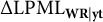 (Nonignorable–Ignorable) when the true missing data mechanisms are nonignorable with large sizes of
$\eta $
(Nonignorable–Ignorable) when the true missing data mechanisms are nonignorable with large sizes of
$\eta $
 s (Simulation Scenario V in red) and nonignorable with small sizes of
$\eta $
s (Simulation Scenario V in red) and nonignorable with small sizes of
$\eta $
 s (Simulation Scenario VI in cyan).

Figure 4 Long description
The chart consists of two vertical panels. The y-axis on both panels is labeled delta L P M L sub W R Y t, ranging from 0 to 200. The left panel is labeled Scenario V and contains a red boxplot centered around 140, with the interquartile range spanning approximately 120 to 150, whiskers extending from about 100 to 200, and several outliers above 150. The right panel is labeled Scenario VI and contains a cyan boxplot centered near zero, with the interquartile range and whiskers close to the baseline, and a few outliers slightly above zero. A dashed red line marks the zero baseline in both panels. Scenario V displays much higher and more dispersed values compared to Scenario VI.
Similarly to Simulation Scenarios I and II, in Table 7 for Simulation Scenario V and Table 8 for Simulation Scenario VI, the biases and SDs of the posterior estimates are relatively small, SDs are similar to RMSEs, and most of the CPs are around the 95% nominal level. Due to the same reason (large missing percentages for the corresponding items) in Simulations I and II, the CP for
$b_{Y7}$
 in Simulation Scenario V and CPs for
$b_{Y4}$
in Simulation Scenario V and CPs for
$b_{Y4}$
 and
$b_{W11}$
and
$b_{W11}$
 in Simulation Scenario VI are lower than the nominal level. These CPs are improved when sample size increases, as shown in Table 10.
Bias, SD, RMSE, and CP of parameters in the item response model, the response time model, and the missing data models under the nonignorable missing data mechanism in Simulation Scenario V (
$n=2,000$
 ,
$J=12$
,
$J=12$
 , large sizes of
$\eta $
, large sizes of
$\eta $
 s, 20% missing data percentage (15% due to omission + 5% due to not-reached), and the true missing data mechanism is nonignorable)

Table 7 Long description
The table presents performance metrics for various parameters across two main vertical sections. Each section contains columns for Parameter, Bias, S D, R M S E, and C P.
* Item Response Parameters (a sub Y 1 to a sub Y 12 and b sub Y 1 to b sub Y 12): Bias values are generally near zero, ranging from minus 0.004 to 0.040. S D and R M S E values range from 0.055 to 0.369. C P values are mostly between 0.930 and 0.962, with b sub Y 7 being an outlier at 0.894.
* Response Time Parameters (a sub T 1 to a sub T 12 and b sub T 1 to b sub T 12): Bias values are extremely low, often 0.000 or 0.001. S D and R M S E values are consistently low, particularly for the b sub T parameters (around 0.016 to 0.030). C P values range from 0.929 to 0.959.
* Missing Data Model Parameters (b sub W 1 to b sub W 12 and b sub R 1 to b sub R 11): The b sub W parameters show higher variability, with S D values reaching up to 0.619 and R M S E up to 0.520. The b sub R parameters are more stable, with S D and R M S E values below 0.156.
* Additional Parameters: Includes sigma sub T (Bias 0.001, C P 0.956), eta sub T (Bias 0.006, C P 0.932), eta sub W (Bias 0.027, C P 0.976), alpha sub W (Bias 0.019, C P 0.954), eta sub R (Bias 0.015, C P 0.956), and alpha sub R (Bias 0.017, C P 0.941).
Bias, SD, RMSE, and CP of parameters in the item response model, the response time model, and the missing data models under the nonignorable missing data mechanism in Simulation Scenario VI (
$n=2,000$
 ,
$J=12$
,
$J=12$
 , small sizes of
$\eta $
, small sizes of
$\eta $
 s, 20% missing data percentage (15% due to omission + 5% due to not-reached), and the true missing data mechanism is nonignorable)

Table 8 Long description
The table presents statistical results for Simulation Scenario VI with n = 2,000 and J = 12. It is organized into two main vertical sections, each containing columns for Parameter, Bias, S D, R M S E, and C P.
* Item Response Parameters (a sub Y and b sub Y): For items 1 through 12, Bias values for a sub Y range from -0.018 to 0.044, while b sub Y Bias values range from -0.008 to 0.246. C P values are generally between 0.911 and 0.965.
* Response Time Parameters (a sub T and b sub T): For items 1 through 12, a sub T Bias values are very low, ranging from -0.005 to 0.005. b sub T Bias values are consistently near 0.000. C P values range from 0.933 to 0.961.
* Missing Data Model Parameters (b sub W and b sub R): For items 1 through 12, b sub W Bias values range from -0.123 to 0.109. b sub R Bias values range from 0.003 to 0.007.
* Latent and Structural Parameters:
- sigma sub T: Bias 0.000, S D 0.008, R M S E 0.009, C P 0.936.
- eta sub T: Bias -0.002, S D 0.039, R M S E 0.038, C P 0.942.
- eta sub W: Bias 0.038, S D 0.112, R M S E 0.106, C P 0.959.
- alpha sub W: Bias 0.676, S D 0.785, R M S E 0.733, C P 0.979.
- eta sub R: Bias 0.026, S D 0.062, R M S E 0.067, C P 0.924.
- alpha sub R: Bias 0.427, S D 0.670, R M S E 0.576, C P 0.974.
5.4 Simulation Scenarios VII and VIII
The purpose of simulations in this section is to investigate the impact of misspecification of the missing data model when the sample size is small (
$n=500$
 ) in Simulation Scenario VII and large (
$n=4, 000$
) in Simulation Scenario VII and large (
$n=4, 000$
 ) in Simulation Scenario VIII, with all other conditions identical to Scenario I.
Similarly, we fit both nonignorable and ignorable models to the simulated nonignorable datasets in Simulation Scenario VII and the simulated ignorable datasets in Simulation Scenario VIII. The boxplots of the differences values
$\text {LPML}_{\mathbf {{W}} \mathbf {{{R}}}|\mathbf {{{y}}} \mathbf {{t}}}$
 (Nonignorable–Ignorable) under these two models are given in Figure 5. All the three boxplots are above 0, indicating that the nonignorable model outperforms the ignorable model when the true missing data mechanism is nonignorable. As sample size increases, the power of
$\text {LPML}_{\mathbf {{W}} \mathbf {{{R}}}|\mathbf {{{y}}} \mathbf {{t}}}$
(Nonignorable–Ignorable) under these two models are given in Figure 5. All the three boxplots are above 0, indicating that the nonignorable model outperforms the ignorable model when the true missing data mechanism is nonignorable. As sample size increases, the power of
$\text {LPML}_{\mathbf {{W}} \mathbf {{{R}}}|\mathbf {{{y}}} \mathbf {{t}}}$
 becomes greater, which is visualized by the boxplots diverging further from the reference line
$y=0$
becomes greater, which is visualized by the boxplots diverging further from the reference line
$y=0$
 . Specifically, the median (IQR) values are 63.86 (55.90, 72.34) for Scenario I, 14.05 (10.33, 18.23) for Scenario VII, and 129.94 (119.49, 140.93) for Scenario VIII.
Boxplots of
$\Delta \text {LPML}_{\mathbf {{W}} \mathbf {{{R}}}|\mathbf {{{y}}} \mathbf {{t}}}$
 (Nonignorable–Ignorable) when the true missing data mechanisms are nonignorable with
$n=2,000$
(Nonignorable–Ignorable) when the true missing data mechanisms are nonignorable with
$n=2,000$
 (Simulation Scenario I = in red), nonignorable with
$n=500$
(Simulation Scenario I = in red), nonignorable with
$n=500$
 (Simulation Scenario VII in green), and nonignorable with
$n=4, 000$
(Simulation Scenario VII in green), and nonignorable with
$n=4, 000$
 (Simulation Scenario VIII in cyan).

Figure 5 Long description
The y-axis is labeled delta L P M L sub W R Y t, ranging from 0 to 200. The left panel, Scenario I, shows a red boxplot with a median near 75, interquartile range from about 60 to 90, and several outliers above 100. The center panel, Scenario VII, displays a green boxplot with a median near 20, interquartile range from about 10 to 30, and outliers up to 50. The right panel, Scenario VIII, presents a cyan boxplot with a median near 125, interquartile range from about 100 to 150, and outliers above 175. All panels share a dashed red baseline at y equals 0.
Similarly to Simulation Scenario I, in Table 9 for Simulation Scenario VII, the biases and SDs of the posterior estimates are relatively small, SDs are similar to RMSEs, and most of the CPs are around the 95% nominal level. Results for CPs are further improved in Table 10 when the sample size is large, with all CPs being around the nominal level. Additionally, SDs and RMSEs in Simulation Scenario VIII (
$n=4,000$
 ) are the smallest, followed by those in Simulation Scenario I (
$n=2,000$
) are the smallest, followed by those in Simulation Scenario I (
$n=2,000$
 ).
).
Bias, SD, RMSE, and CP of parameters in the item response model, the response time model, and the missing data models under the nonignorable missing data mechanism in Simulation Scenario VII (
$n=500$
 ,
$J=12$
,
$J=12$
 , median sizes of
$\eta $
, median sizes of
$\eta $
 s, 20% missing data percentage (15% due to omission + 5% due to not-reached), and the true missing data mechanism is nonignorable)

Table 9 Long description
The table presents simulation results for various parameters.
Item Response Model Parameters (a sub Y and b sub Y 1 through 12):
* a sub Y 1: Bias -0.037, S D 0.176, R M S E 0.171, C P 0.951.
* b sub Y 1: Bias 0.066, S D 0.262, R M S E 0.234, C P 0.955.
* Values continue through index 12, with b sub Y 7 showing a higher Bias of 0.575 and R M S E of 0.663.
Response Time Model Parameters (a sub T and b sub T 1 through 12):
* a sub T 1: Bias -0.009, S D 0.207, R M S E 0.206, C P 0.939.
* b sub T 1: Bias 0.003, S D 0.039, R M S E 0.038, C P 0.955.
* These parameters generally show lower Bias and R M S E compared to the Y parameters.
Missing Data Model Parameters (b sub W, b sub R, eta, alpha, and sigma):
* b sub W 1: Bias -0.148, S D 0.950, R M S E 0.694, C P 0.956.
* b sub R 1: Bias 0.009, S D 0.118, R M S E 0.120, C P 0.932.
* sigma sub T: Bias 0.002, S D 0.017, R M S E 0.017, C P 0.943.
* eta sub T: Bias 0.012, S D 0.073, R M S E 0.077, C P 0.923.
* alpha sub W: Bias 0.145, S D 0.691, R M S E 0.297, C P 0.990.
* alpha sub R: Bias 0.052, S D 0.200, R M S E 0.195, C P 0.948.
Bias, SD, RMSE, and CP of parameters in the item response model, the response time model, and the missing data models under the nonignorable missing data mechanism in Simulation Scenario VIII (
$n=4,000$
 ,
$J=12$
,
$J=12$
 , median sizes of
$\eta $
, median sizes of
$\eta $
 s, 20% missing data percentage (15% due to omission + 5% due to not-reached), and the true missing data mechanism is nonignorable)

Table 10 Long description
The table presents statistical performance metrics for various parameters.
* Item Response Model Parameters (a sub Y 1 to a sub Y 12 and b sub Y 1 to b sub Y 12): Bias values range from -0.007 to 0.033 for ‘a’ parameters and -0.005 to 0.160 for ‘b’ parameters. C P values are generally between 0.922 and 0.967.
* Response Time Model Parameters (a sub T 1 to a sub T 12 and b sub T 1 to b sub T 12): Bias values are very low, ranging from -0.003 to 0.003. C P values range from 0.935 to 0.957.
* Missing Data Model Parameters (b sub W 1 to b sub W 12 and b sub R 1 to b sub R 11): ‘b sub W’ parameters show higher R M S E values (up to 0.420) compared to ‘b sub R’ parameters (up to 0.110).
* Latent and Variance Parameters:
- sigma sub T: Bias 0.000, S D 0.008, R M S E 0.008, C P 0.940.
- eta sub T: Bias 0.002, S D 0.026, R M S E 0.026, C P 0.940.
- eta sub W: Bias 0.015, S D 0.073, R M S E 0.078, C P 0.928.
- alpha sub W: Bias 0.042, S D 0.230, R M S E 0.195, C P 0.959.
- eta sub R: Bias 0.002, S D 0.032, R M S E 0.033, C P 0.934.
- alpha sub R: Bias 0.007, S D 0.064, R M S E 0.065, C P 0.937.
5.5 Simulation Scenario IX
The purpose of simulations in this section is to investigate the impact of misspecification of the missing data model when the missing data percentages of the simulated datasets are around 20% (5% due to omission behavior and 15% due to not-reached behavior). The proportions of missing percentage are different from those in Simulation Scenario I (15% is due to omission and 5% is due to not-reached behavior). Other conditions are identical to Scenario I.
We fit both nonignorable and ignorable models to the simulated nonignorable datasets in Simulation Scenario IX. The boxplot of difference values
$\text {LPML}_{\mathbf {{W}} \mathbf {{{R}}}|\mathbf {{{y}}} \mathbf {{t}}}$
 (Nonignorable–Ignorable) under these two models is given in Figure 6. All the two boxplots are above 0, indicating that the nonignorable model outperforms the ignorable model when the true missing data mechanism is nonignorable. The power of
$\text {LPML}_{\mathbf {{W}} \mathbf {{{R}}}|\mathbf {{{y}}} \mathbf {{t}}}$
(Nonignorable–Ignorable) under these two models is given in Figure 6. All the two boxplots are above 0, indicating that the nonignorable model outperforms the ignorable model when the true missing data mechanism is nonignorable. The power of
$\text {LPML}_{\mathbf {{W}} \mathbf {{{R}}}|\mathbf {{{y}}} \mathbf {{t}}}$
 in Simulation Scenario I is greater than that in Simulation Scenario IX, which is visualized by the boxplots diverging further from the reference line
$y=0$
in Simulation Scenario I is greater than that in Simulation Scenario IX, which is visualized by the boxplots diverging further from the reference line
$y=0$
 . Specifically, the median (IQR) values are 63.86 (55.90, 72.34) for Scenario I and 39.20 (33.58, 45.33) for Scenario IX.
Boxplots of
$\Delta \text {LPML}_{\mathbf {{W}} \mathbf {{{R}}}|\mathbf {{{y}}} \mathbf {{t}}}$
 (Nonignorable–Ignorable) when the true missing data mechanisms are nonignorable (Simulation Scenario I in red) and nonignorable (Simulation Scenario IX in cyan).

Figure 6 Long description
The chart contains two vertical boxplots. The y-axis is labeled delta L P M L sub W R Y vertical bar t, ranging from 0 to above 100. The left boxplot, shaded red and labeled Scenario I, has a median near 70, interquartile range from about 60 to 80, whiskers extending from about 40 to 100, and several outliers above 100. The right boxplot, shaded cyan and labeled Scenario I X, has a median near 50, interquartile range from about 40 to 60, whiskers from about 20 to 90, and multiple outliers above 90. Both boxplots are above a dashed red horizontal line at y equals 0.
Similarly to Simulation Scenario I, in Table 11 for Simulation Scenario IX, the biases and SDs of the posterior estimates are relatively small, SDs are similar to RMSEs, and most of the CPs are around the 95% nominal level. SDs and RMSEs of W model in Simulation Scenario IX are smaller than those in Simulation Scenario I. SDs and RMSEs of R model in Simulation Scenario IX are greater than those in Simulation Scenario I. Both results are expected given that we have more missingness due to not-reached and less missingness due to omission in Scenario IX.
Bias, SD, RMSE, and CP of parameters in the item response model, the response time model, and the missing data models under the nonignorable missing data mechanism in Simulation Scenario IX (
$n=2,000$
 ,
$J=12$
,
$J=12$
 , median sizes of
$\eta $
, median sizes of
$\eta $
 s, 20% missing data percentage (5% due to omission + 15% due to not-reached), and the true missing data mechanism is nonignorable)

Table 11 Long description
The table is organized into two main sections of five columns each, both containing headers for Parameter, Bias, S D, R M S E, and C P.
Item Response Model Parameters:
* a sub Y 1 to a sub Y 12: Bias ranges from minus 0.013 to 0.037. S D ranges from 0.067 to 0.114. R M S E ranges from 0.064 to 0.114. C P ranges from 0.931 to 0.968.
* b sub Y 1 to b sub Y 12: Bias ranges from minus 0.004 to 0.178. S D ranges from 0.085 to 0.288. R M S E ranges from 0.088 to 0.296. C P ranges from 0.918 to 0.961.
Response Time Model Parameters:
* a sub T 1 to a sub T 12: Bias ranges from minus 0.006 to 0.005. S D ranges from 0.057 to 0.132. R M S E ranges from 0.059 to 0.133. C P ranges from 0.936 to 0.964.
* b sub T 1 to b sub T 12: Bias ranges from minus 0.002 to 0.000. S D ranges from 0.016 to 0.025. R M S E ranges from 0.015 to 0.025. C P ranges from 0.935 to 0.960.
Missing Data Model Parameters:
* b sub W 1 to b sub W 12: Bias ranges from minus 0.049 to 0.052. S D ranges from 0.084 to 0.399. R M S E ranges from 0.081 to 0.375. C P ranges from 0.939 to 0.960.
* b sub R 1 to b sub R 11: Bias ranges from minus 0.050 to 0.019. S D ranges from 0.067 to 0.316. R M S E ranges from 0.067 to 0.316. C P ranges from 0.938 to 0.954.
Latent and Variance Parameters:
* sigma sub T: Bias 0.000, S D 0.008, R M S E 0.008, C P 0.940.
* eta sub T: Bias 0.002, S D 0.036, R M S E 0.037, C P 0.936.
* eta sub W: Bias 0.018, S D 0.100, R M S E 0.108, C P 0.913.
* alpha sub W: Bias 0.068, S D 0.346, R M S E 0.243, C P 0.959.
* eta sub R: Bias 0.001, S D 0.060, R M S E 0.058, C P 0.947.
* alpha sub R: Bias 0.022, S D 0.119, R M S E 0.124, C P 0.936.
Posterior summaries remain good for the parameters of R model even when the percentage of missingness due to omission is small (5%) in Simulation Scenario IX and for the parameters of W model even when the percentage of missingness due to not-reached is small (5%) in Simulation Scenario I. This indicates that our methods perform robustly when the missing data percentages for both omission and not-reached are small.
6 Analysis of the PISA 2018 Test Data
6.1 Data overview
The PISA 2018 math exam in Brazil includes six test booklets. The percentages of missing items for each booklet are 18.6%, 10.9%, 13.0%, 14.1%, 13.6%, and 16.8%, respectively. In our real data analysis, we focus on the first test, which comprises 1,742 records (
$n = 1,742$
 ) and 12 items (
$J = 12$
) and 12 items (
$J = 12$
 ). The total time limit is 60 minutes. The percentage of missing items (
$\mathbf{R}$
). The total time limit is 60 minutes. The percentage of missing items (
$\mathbf{R}$
 ) is 18.6% (12.3% due to omission and 6.3% due to not-reached) and the percentage of not-reached behavior (
$\mathbf{W}$
) is 18.6% (12.3% due to omission and 6.3% due to not-reached) and the percentage of not-reached behavior (
$\mathbf{W}$
 ) is 18.7%. Table 12 shows the not-reached and omitted behaviors, where the
$(i, j)$
) is 18.7%. Table 12 shows the not-reached and omitted behaviors, where the
$(i, j)$
 th element represents the total number of missing answers for item j among subjects who fail to reach item i. The lower triangular matrix in red and bold font then shows the number of omitted items for item j among subjects who fail to reach item i, for
$j \le i-2$
th element represents the total number of missing answers for item j among subjects who fail to reach item i. The lower triangular matrix in red and bold font then shows the number of omitted items for item j among subjects who fail to reach item i, for
$j \le i-2$
 . Each row total for
$W\le 12$
. Each row total for
$W\le 12$
 returns the total number of subjects that fail to reach the corresponding item, which is the same as the corresponding diagonal element. Each column total returns the total number of missing answers for that item, with the total number of omitted items in parentheses and in red and bold font. Table 13 presents a summary of the response accuracy and response times for each item.
The not-reached and omitted behaviors in PISA 2018 test data: the
$(i, j)$
 th element represents the total number of missing answers for item j among subjects who fail to reach item i

Table 12 Long description
Starting from the top row, the leftmost column lists item numbers from 1 to 13. Each row corresponds to subjects who failed to reach a specific item, and each cell across columns 1 to 13 shows the number of missing answers for item j among those who did not reach item i. For example, row 2 shows 7 missing answers for items 2 to 12, row 3 shows 17 missing answers for items 3 to 12, and row 5 shows 28 missing answers for item 3 and 32 for items 5 to 12. Bold values highlight omitted behaviors. The final column in each row gives the total missing answers for that item. The bottom rows summarize omitted counts in parentheses and total missingness per item, with the highest missing counts in item 13 (1,417) and item 5 (701).
6.2 Posterior estimation
We fit the data using the proposed item response and response time models proposed in Section 2, together with both nonignorable and ignorable (i.e., set
$\eta _W=\eta _R=0$
 ) missing data mechanisms proposed in Section 3. We evaluate the convergence of models using traceplots and autocorrelation plots, as shown in the Supplementary Material. All plots indicate good mixing of the chains and convergence for all parameters. We define a posterior estimate to be “statistically significant at a significance level of 0.05” if the corresponding 95% HPD interval does not include 0.
Table 14 presents the posterior summaries of the difficulty parameters in the response model, that is,
$a_{Yj}b_{Yj}$
 , where a larger value indicates that the
$j^{\text {th}}$
, where a larger value indicates that the
$j^{\text {th}}$
 item is more difficult and its answer is more likely wrong. For example,
$a_{Y1}b_{Y1}=-0.759 $
item is more difficult and its answer is more likely wrong. For example,
$a_{Y1}b_{Y1}=-0.759 $
 (
$95\%~\text {HPD} =(-0.883, -0.642)$
(
$95\%~\text {HPD} =(-0.883, -0.642)$
 ) is the smallest significant value reported in Table 14, which is consistent with the fact that Item 1 has the highest percentage of correct answers as shown in Table 13.
$a_{Y9}b_{Y9}=5.062$
) is the smallest significant value reported in Table 14, which is consistent with the fact that Item 1 has the highest percentage of correct answers as shown in Table 13.
$a_{Y9}b_{Y9}=5.062$
 (
$95\%~\text {HPD} =(4.400, 45.958)$
(
$95\%~\text {HPD} =(4.400, 45.958)$
 ) and
$a_{Y11}b_{Y11}=5.366$
) and
$a_{Y11}b_{Y11}=5.366$
 (
$95\%~\text {HPD} =(4.629, 6.300)$
(
$95\%~\text {HPD} =(4.629, 6.300)$
 ) are the first and second highest values, which aligns well with the fact that these two items have the smallest percentages of correctness in Table 13.
The total number of observed answers (
$n_{\text {obs}}$
 ), the number and percentage of correct answers, the median, the first quartile (
$Q_1$
), the number and percentage of correct answers, the median, the first quartile (
$Q_1$
 ), and the third quartile (
$Q_3$
), and the third quartile (
$Q_3$
 ) of response times (in minutes) for each item

Table 13 Long description
From left to right, columns are labeled Item 1 through Item 12. The first row lists the total observed answers: 1,704, 1,718, 1,149, 1,383, 1,041, 1,599, 1,474, 1,581, 1,486, 1,321, 1,143, 1,417. The second row shows correct answers: 1,129, 651, 554, 714, 197, 514, 194, 441, 67, 148, 31, 198. The third row gives percentages: 66.26, 37.89, 48.22, 51.63, 18.92, 32.15, 13.16, 27.89, 4.51, 11.20, 2.71, 13.97. The fourth row presents medians: 8.64, 10.07, 29.54, 14.38, 19.65, 14.38, 27.46, 9.56, 16.79, 27.22, 13.49, 15.69. The fifth row shows first quartiles: 6.22, 7.39, 17.65, 8.63, 9.09, 9.38, 17.93, 5.98, 12.23, 19.05, 8.46, 10.24. The sixth row lists third quartiles: 12.58, 14.86, 47.32, 21.40, 35.71, 20.03, 38.95, 14.01, 24.12, 37.36, 22.37, 22.28. Correct answer percentages and response times vary widely across items, with Item 1 showing the highest accuracy and Item 11 the lowest.
Mean, SD, and 95% HPD of the difficulty parameters in the item response model under the nonignorable missing data mechanism

Table 14 Long description
From top to bottom, the table lists parameter names in the leftmost column: Y sub 1, Y sub 2, Y sub 3, Y sub 4, Y sub 5, Y sub 6, Y sub 7, Y sub 8, Y sub 9, b sub Y 10, b sub Y 11, b sub Y 12. The next column to the right shows mean values: negative 0.759, 0.631, 0.612, 0.191, 2.007, 1.001, 3.315, 0.977, 5.062, 3.640, 5.366, 2.389. The third column displays standard deviations: 0.065, 0.063, 0.117, 0.080, 0.122, 0.075, 0.243, 0.060, 0.414, 0.285, 0.455, 0.129. The rightmost column gives 95 percent H P D intervals: negative 0.883 to negative 0.642, 0.501 to 0.748, 0.390 to 0.836, 0.022 to 0.337, 1.797 to 2.266, 0.846 to 1.146, 2.879 to 3.775, 0.868 to 1.108, 4.400 to 5.958, 3.143 to 4.226, 4.629 to 6.300, 2.155 to 2.651. Each row corresponds to a unique parameter and its associated statistics under the nonignorable missing data mechanism.
According to Table 15,
$b_{T3}=3.125$
 (
$95\%~\text {HPD} =(3.066, 3.186)$
(
$95\%~\text {HPD} =(3.066, 3.186)$
 ),
$b_{T7}=3.088$
),
$b_{T7}=3.088$
 (
$95\%~\text {HPD} =(3.036, 3.147)$
(
$95\%~\text {HPD} =(3.036, 3.147)$
 ), and
$b_{T10}=3.209$
), and
$b_{T10}=3.209$
 (
$95\%~\text {HPD} =(3.179, 3.242)$
(
$95\%~\text {HPD} =(3.179, 3.242)$
 ) are the three significant parameters with the highest values among all items. This aligns well with the findings in Table 13, where students tend to spend more time on Items 3, 7, and 10.
$b_{R3}=0.872 $
) are the three significant parameters with the highest values among all items. This aligns well with the findings in Table 13, where students tend to spend more time on Items 3, 7, and 10.
$b_{R3}=0.872 $
 (
$95\%~\text {HPD} =(0.749, 1.008)$
(
$95\%~\text {HPD} =(0.749, 1.008)$
 ) and
$b_{R5}=0.584$
) and
$b_{R5}=0.584$
 (
$95\%~\text {HPD} =(0.457, 0.718)$
(
$95\%~\text {HPD} =(0.457, 0.718)$
 ) are the two significant parameters with the smallest values among all items, which is consistent with the fact that the total numbers of omitted missingness of Items 3 and 5 are the greatest. Additionally, Table 15 shows that
$\eta _{T}=-0.377 $
) are the two significant parameters with the smallest values among all items, which is consistent with the fact that the total numbers of omitted missingness of Items 3 and 5 are the greatest. Additionally, Table 15 shows that
$\eta _{T}=-0.377 $
 (
$95\%~\text {HPD} =(-0.438, -0.309)$
(
$95\%~\text {HPD} =(-0.438, -0.309)$
 ) has a negative significant effect, indicating that subjects tend to spend less time if their latent propensities are low.
$\eta _W=-0.275$
) has a negative significant effect, indicating that subjects tend to spend less time if their latent propensities are low.
$\eta _W=-0.275$
 (
$95\%~\text {HPD} =(-0.450, -0.093)$
(
$95\%~\text {HPD} =(-0.450, -0.093)$
 ),
$\alpha _W=1.274$
),
$\alpha _W=1.274$
 (
$95\%~\text {HPD} =(0.666, 1.909)$
(
$95\%~\text {HPD} =(0.666, 1.909)$
 ),
$\eta _R=-0.462$
),
$\eta _R=-0.462$
 (
$95\%~\text {HPD} =(-0.530, -0.391)$
(
$95\%~\text {HPD} =(-0.530, -0.391)$
 ), and
$\alpha _R=1.713$
), and
$\alpha _R=1.713$
 (
$95\%~\text {HPD} =(1.552, 1.885)$
(
$95\%~\text {HPD} =(1.552, 1.885)$
 ) are all significantly different from 0, indicating that the missing data mechanism may be nonignorable, which is consistent with the
$\text {LPML}_{\mathbf {{W}} \mathbf {{{R}}}|\mathbf {{{y}}} \mathbf {{t}}}$
) are all significantly different from 0, indicating that the missing data mechanism may be nonignorable, which is consistent with the
$\text {LPML}_{\mathbf {{W}} \mathbf {{{R}}}|\mathbf {{{y}}} \mathbf {{t}}}$
 model selection criterion in Section 6.3 and the statements in Glas and Pimentel (Reference Glas and Pimentel2008) and Rose et al. (Reference Rose, von Davier and Nagengast2017). Additionally,
$\sigma _T=0.390$
model selection criterion in Section 6.3 and the statements in Glas and Pimentel (Reference Glas and Pimentel2008) and Rose et al. (Reference Rose, von Davier and Nagengast2017). Additionally,
$\sigma _T=0.390$
 (
$95\%~\text {HPD} =(0.374, 0.404)$
(
$95\%~\text {HPD} =(0.374, 0.404)$
 ).
).
Mean, SD, and 95% HPD of discrimination parameters and difficulty parameters in the item response model, item time intensity parameters and discrimination parameters in the response time model, difficulty parameters for the not-reached behavior, difficulty parameters for the omitted behavior, and the formulation parameters under the nonignorable missing data mechanism

Table 15 Long description
The table is organized into two main sections of four columns each. The columns are Parameter, Mean, S D, and 95% H P D.
* Item Response Model Parameters (a sub Y 1 to a sub Y 12 and b sub Y 1 to b sub Y 12): a sub Y values range from 0.346 to 2.268. b sub Y values range from minus 0.878 to 2.898.
* Response Time Model Parameters (a sub T 1 to a sub T 12 and b sub T 1 to b sub T 12): a sub T values range from 0.659 to 5.427. b sub T values range from 2.123 to 3.209.
* Not-reached Behavior Difficulty Parameters (b sub W 1 to b sub W 12): Values range from 3.429 to 8.491.
* Omitted Behavior Difficulty Parameters (b sub R 1 to b sub R 11): Values range from 0.584 to 5.236.
* Formulation and Variance Parameters:
- sigma sub T: Mean 0.390, S D 0.008, H P D (0.374, 0.404).
- eta sub T: Mean minus 0.377, S D 0.034, H P D (minus 0.438, minus 0.309).
- eta sub W: Mean minus 0.275, S D 0.093, H P D (minus 0.450, minus 0.093).
- alpha sub W: Mean 1.274, S D 0.299, H P D (0.666, 1.909).
- eta sub R: Mean minus 0.462, S D 0.037, H P D (minus 0.530, minus 0.391).
- alpha sub R: Mean 1.713, S D 0.085, H P D (1.552, 1.885).
According to Table 16, the correlation of the latent propensities between the item response and the not-reached behavior, measured by
$\eta _W sin (\alpha _W)=-0.252$
 (
$95\%~\text {HPD} =(-0.423, -0.081)$
(
$95\%~\text {HPD} =(-0.423, -0.081)$
 ) is significant, indicating that subjects with better latent abilities tend not to withdraw the test. The correlation of the latent propensities between the response time and the not-reached behavior, measured by
$\eta _W (\eta _T \text {sin} (\alpha _W)+ \sqrt {1-(\eta _T)^2} \text {cos} (\alpha _W))=0.018$
) is significant, indicating that subjects with better latent abilities tend not to withdraw the test. The correlation of the latent propensities between the response time and the not-reached behavior, measured by
$\eta _W (\eta _T \text {sin} (\alpha _W)+ \sqrt {1-(\eta _T)^2} \text {cos} (\alpha _W))=0.018$
 (
$95\%~\text {HPD} =(-0.126, 0.151) $
(
$95\%~\text {HPD} =(-0.126, 0.151) $
 ) is insignificant. We then calculate the correlation of latent propensities between the item response and the omitted behavior, measured by
$\eta _R sin (\alpha _R)=-0.456$
) is insignificant. We then calculate the correlation of latent propensities between the item response and the omitted behavior, measured by
$\eta _R sin (\alpha _R)=-0.456$
 (
$95\%~\text {HPD} =(-0.524, -0.382)$
(
$95\%~\text {HPD} =(-0.524, -0.382)$
 ), indicating that subjects with better latent abilities tend not to omit items. We further compute the correlation of latent propensities between the response time and the omitted behavior, measured by
$\eta _R (\eta _T \text {sin} (\alpha _R)+ \sqrt {1-(\eta _T)^2} \text {cos} (\alpha _R))=0.232$
), indicating that subjects with better latent abilities tend not to omit items. We further compute the correlation of latent propensities between the response time and the omitted behavior, measured by
$\eta _R (\eta _T \text {sin} (\alpha _R)+ \sqrt {1-(\eta _T)^2} \text {cos} (\alpha _R))=0.232$
 (
$95\%~\text {HPD} =(0.164, 0.286) $
(
$95\%~\text {HPD} =(0.164, 0.286) $
 ). The positive signficant value indicates that subjects with longer response times tend to omit items.
Mean, SD, and 95% HPD of computed parameters under the nonignorable missing data mechanism

Table 16 Long description
Starting from the top row, the first parameter is eta sub W times sine of alpha sub W, with mean negative 0.252, S D 0.088, and 95 percent H P D from negative 0.423 to negative 0.081. The second parameter is eta sub W times open parenthesis eta sub T times sine of alpha sub W plus square root of 1 minus open parenthesis eta sub T close parenthesis squared times cosine of alpha sub W close parenthesis, with mean 0.018, S D 0.070, and 95 percent H P D from negative 0.126 to 0.151. The third parameter is eta sub R times sine of alpha sub R, with mean negative 0.456, S D 0.039, and 95 percent H P D from negative 0.524 to negative 0.382. The fourth parameter is eta sub R times open parenthesis eta sub T times sine of alpha sub R plus square root of 1 minus open parenthesis eta sub T close parenthesis squared times cosine of alpha sub R close parenthesis, with mean 0.232, S D 0.031, and 95 percent H P D from 0.164 to 0.286.
We also present the posterior summaries under the ignorable missing data mechanism in Table 17, some of which are quite different from the posterior summaries under the nonignorable missing data mechanism in Table 15. For example,
$b_{Y4}=0.120$
 is significant under the nonignorable missing data mechanism (
$95\%~\text {HPD} =(0.015, 0.211$
is significant under the nonignorable missing data mechanism (
$95\%~\text {HPD} =(0.015, 0.211$
 ) but is not significant under the ignorable missing data mechanism
$b_{Y4}=0.035$
) but is not significant under the ignorable missing data mechanism
$b_{Y4}=0.035$
 (
$95\%~\text {HPD} =(-0.072, 0.126)$
(
$95\%~\text {HPD} =(-0.072, 0.126)$
 ).
).
Mean, SD, and 95% HPD of discrimination parameters and difficulty parameters in the item response model, item time intensity parameters and discrimination parameters in the response time model, difficulty parameters for the not-reached behavior, and difficulty parameters for the omitted behavior under the ignorable missing data mechanism

Table 17 Long description
Starting from the top row, the table displays two sets of columns for each parameter: the left set includes parameter, mean, standard deviation, and 95 percent highest posterior density; the right set repeats these for a second parameter. Parameters are labeled as a sub Y 1 through a sub Y 12, b sub Y 1 through b sub Y 12, a sub T 10 through a sub T 12, b sub T 10 through b sub T 12, a sub V 1 through a sub V 5, b sub V 1 through b sub V 5, a sub I 1 through a sub I 5, b sub I 1 through b sub I 5, b sub W 10 through b sub W 12, b sub R 10 through b sub R 12, and sigma sub T. For each parameter, the mean, standard deviation, and 95 percent highest posterior density interval are listed. For example, a sub Y 1 has mean 0.978, standard deviation 0.094, and interval (0.800, 1.183); b sub Y 1 has mean negative 0.813, standard deviation 0.085, and interval (negative 0.991, negative 0.655). The table continues in this format for all parameters, providing detailed statistical estimates for item response model discrimination and difficulty, item time intensity and discrimination in the response time model, difficulty for not-reached and omitted behaviors, and ignorable missing data mechanism.
6.3 Model comparison
We first use the LPML decomposition technique developed in Section 4.3 to guide the selection of the missing data mechanism. The
$\text {LPML}_{\mathbf {{W}} \mathbf {{{R}}}|\mathbf {{{y}}} \mathbf {{t}}}$
 (
$-$
(
$-$
 6943.24) under the nonignorable missing data mechanism is greater than the
$\text {LPML}_{\mathbf {{W}} \mathbf {{{R}}}}$
6943.24) under the nonignorable missing data mechanism is greater than the
$\text {LPML}_{\mathbf {{W}} \mathbf {{{R}}}}$
 (
$-$
(
$-$
 7026.59) under the ignorable missing data mechanism, indicating that the nonignorable missing data mechanism is more favorable for this dataset. The posterior summaries under the nonignorable missing data mechanism are given in Tables 14 and 15.
To further evaluate the significance of the joint model for item response (
$\mathbf {{{y}}}$
 ) and response time (
$\mathbf {{t}}$
) and response time (
$\mathbf {{t}}$
 ) in identifying the missing data mechanism, we compare it with the single outcome model for
$\mathbf {{{y}}}$
) in identifying the missing data mechanism, we compare it with the single outcome model for
$\mathbf {{{y}}}$
 in (19) and the single outcome model for
$\mathbf {{t}}$
in (19) and the single outcome model for
$\mathbf {{t}}$
 in (20) under the nonignorable missing data mechanism, respectively. The
$\text {LPML}_{ \mathbf {{W}} \mathbf {{{R}}}|\mathbf {{{y}}} }$
in (20) under the nonignorable missing data mechanism, respectively. The
$\text {LPML}_{ \mathbf {{W}} \mathbf {{{R}}}|\mathbf {{{y}}} }$
 (
$-$
(
$-$
 6957.56) for the
$\mathbf {{{y}}}$
6957.56) for the
$\mathbf {{{y}}}$
 -only model and the
$\text {LPML}_{ \mathbf {{W}} \mathbf {{{R}}}|\mathbf {{t}} }$
-only model and the
$\text {LPML}_{ \mathbf {{W}} \mathbf {{{R}}}|\mathbf {{t}} }$
 (
$-$
(
$-$
 6999.81) for the
$\mathbf {{t}}$
6999.81) for the
$\mathbf {{t}}$
 -only model are smaller than that for the joint model, indicating that the joint model provides better identification of the missing data mechanism compared to the two single outcome models.
We further compare our methods with MICE with 20 imputations. We apply the same item response and response time models in (1) and (2) for each imputed data set for fair comparison. Table 18 shows the final posterior summaries obtained after pooling. Most results are similar except for
$b_{Y4}$
 , which is not significant under MICE but is significant under the proposed nonignorable missing data models. The computation time under MICE (274.87 minutes) is substantially longer than that of the proposed model (49.00 minutes). Additionally, the omission and not-reached behaviors are not studied in the MICE approach. We also compare our methods with the RTprocess model in Table 19. For fair comparison, we assume the same hierarchical framework and reparameterization technique for
${{{\theta }}}$
, which is not significant under MICE but is significant under the proposed nonignorable missing data models. The computation time under MICE (274.87 minutes) is substantially longer than that of the proposed model (49.00 minutes). Additionally, the omission and not-reached behaviors are not studied in the MICE approach. We also compare our methods with the RTprocess model in Table 19. For fair comparison, we assume the same hierarchical framework and reparameterization technique for
${{{\theta }}}$
 and
${{ {\theta }}}_T$
and
${{ {\theta }}}_T$
 , which guarantees that the covariance matrix is positive definite. Similarly to MICE,
$b_{Y4}$
, which guarantees that the covariance matrix is positive definite. Similarly to MICE,
$b_{Y4}$
 is not significant under the RTprocess model but is significant under the proposed nonignorable missing data models.
$\eta _T$
is not significant under the RTprocess model but is significant under the proposed nonignorable missing data models.
$\eta _T$
 and
$\sigma _T$
and
$\sigma _T$
 are similar to those obtained in the proposed model. However, similar to MICE, the omission and not-reached behaviors are not modeled directly.
Mean, SD, and 95% HPD of discrimination parameters and difficulty parameters in the item response model and item time intensity parameters and discrimination parameters in the response time model under MICE

Table 18 Long description
The table contains two sets of columns for each row: the left set for item response model parameters and the right set for response time model parameters. Each set includes parameter name, mean, standard deviation, and 95 percent highest posterior density interval. For the item response model, parameters a sub Y 1 to a sub Y 12, a sub T 10 to a sub T 12, sigma sub T, and eta sub T are listed. For example, a sub Y 1 has mean 0.941, standard deviation 0.093, and 95 percent H P D interval 0.764 to 1.131. The corresponding b sub Y 1 parameter in the response time model has mean negative 0.834, standard deviation 0.090, and 95 percent H P D interval negative 1.025 to negative 0.672. This pattern continues for all parameter pairs, with values such as a sub Y 2 mean 1.151, standard deviation 0.096, 95 percent H P D 0.974 to 1.348; b sub Y 2 mean 0.553, standard deviation 0.063, 95 percent H P D 0.437 to 0.682. The highest mean values are observed for a sub T 10 at 4.955 and b sub Y 5 at 2.233. The lowest mean values are for a sub Y 5 at 0.333 and b sub Y 4 at 0.046. The table concludes with sigma sub T mean 0.392, standard deviation 0.009, 95 percent H P D 0.376 to 0.409, and eta sub T mean negative 0.369, standard deviation 0.033, 95 percent H P D negative 0.432 to negative 0.304.
Mean, SD, and 95% HPD of discrimination parameters and difficulty parameters in the item response model and item time intensity parameters and discrimination parameters in the response time model under the response time process model

Table 19 Long description
The table contains two sets of columns for each row: the left set for item response model parameters and the right set for response time model parameters. Each set includes Parameter, Mean, Standard Deviation, and 95 percent Highest Posterior Density (HPD) interval. From top to bottom, the item response model parameters a sub Y 1 to a sub Y 12, a sub T 10 to a sub T 12, sigma sub T, and eta sub T are listed with their corresponding means, standard deviations, and HPD intervals. For example, a sub Y 1 has mean 0.954, standard deviation 0.092, HPD (0.786, 1.143). The response time model parameters b sub Y 1 to b sub Y 12, b sub T 10 to b sub T 12 are similarly listed. For example, b sub Y 1 has mean negative 0.838, standard deviation 0.086, HPD (negative 1.004, negative 0.673). The table provides a comprehensive summary of parameter estimates for both models, allowing direct comparison of discrimination and difficulty across items and models.
Finally, we compare the estimations and inferences of the ability parameters across different models. The stacked bar charts in Figure 7 show the counts of significant and insignificant ability parameter estimates
$\hat { {\theta }}$
 , grouped by the number of missing items. The bars represent negative significant estimates with 95% HPD intervals that are entirely below zero in blue, positive significant estimates with 95% HPD intervals that are entirely above zero in green, and insignificant estimates with 95% HPD intervals including zero in red. We see from Figure 7 that there are lower (higher) proportions of “blue” and higher (lower) proportions of “green” among the bars for small (large) numbers of missing items under the proposed nonignorable model than the other three methods. The results under the nonignorable model are more desirable and intuitively appealing since the subjects with higher (lower) abilities are more likely to have fewer (more) missing items. Table 20 presents the minimum (Min), first quartile (Q1), median (Q2), third quartile (Q3), and maximum (Max) of the posterior means of the latent traits across different models. The proposed nonignorable model has the largest values of IQR (Q3–Q1) and range (Max–Min). Thus, the nonignorable model can distinguish the subjects’ abilities more effectively.
Stacked bar charts showing the number of significant and insignificant ability parameter estimates across different methods, grouped by the number of missing items. Blue bars correspond to the negative significant
$\hat { {\theta }}$
 , green bars correspond to the positive significant
$\hat { {\theta }}$
, green bars correspond to the positive significant
$\hat { {\theta }}$
 , and red bars correspond to the insignificant
$\hat { {\theta }}$
, and red bars correspond to the insignificant
$\hat { {\theta }}$
 .
.

Figure 7 Long description
From left to right, the panels are labeled Nonignorable, Ignorable, M I C E, and R T process. Each panel displays stacked vertical bars for number of missing items on the x axis, ranging from 0 to 12, and count on the y axis, ranging from 0 to over 600. Each bar is divided into three color-coded segments: blue for negative significant, green for positive significant, and red for insignificant ability parameter estimates. In all panels, the highest counts occur at zero missing items, dominated by red (insignificant) segments, followed by green (positive significant) and a small blue (negative significant) segment. As the number of missing items increases, the total count decreases, with the red segment remaining the largest proportion in each bar. The distribution pattern is similar across all four methods.
Minimum, first quartile, median, third quartile, and maximum of the posterior means of the ability parameters

Table 20 Long description
Starting from the top row, the Nonignorable method shows minimum negative 2.602, first quartile negative 0.651, median negative 0.070, third quartile 0.607, and maximum 2.871. The Ignorable method has minimum negative 1.347, first quartile negative 0.636, median negative 0.080, third quartile 0.511, and maximum 2.884. The M I C E method presents minimum negative 2.171, first quartile negative 0.614, median negative 0.066, third quartile 0.523, and maximum 2.759. The R T process method lists minimum negative 2.176, first quartile negative 0.657, median negative 0.057, third quartile 0.586, and maximum 2.842. Each row corresponds to a method, and each column represents a statistical summary of the posterior means of ability parameters.
Figure 8 shows the differences between ability estimates under the proposed nonignorable model and the competing models as a function of the response time propensity estimates under the proposed nonignorable model. Data points with darker color correspond to subjects with more missing items. Among all the competing approaches, MICE provides the most different results. The ability estimates under the proposed nonignorable model tend to be smaller than those under the proposed ignorable model when the number of missing items is high and when the response time propensity estimate is large. This suggests that the missing data process influences the analysis of outcome models, indicating that the missing data mechanism may be nonignorable. The ability estimates under the proposed nonignorable model tend to be smaller than those under the RTprocess model for subjects with more missing items. The results are consistent with intuition that subjects with higher (lower) abilities are more likely to have fewer (more) missing items.
Difference in the ability estimates between the proposed nonignorable model and the competing models plotted against the response time propensity estimates under the proposed nonignorable model. The number of missing values is given by the data points’ color, with darker colors denoting a higher number of missingness.

Figure 8 Long description
There are three adjacent scatterplots. The left panel is labeled theta Y Nonign minus theta Y Ign. The middle panel is labeled theta Y Nonign minus theta Y M I C E. The right panel is labeled theta Y Nonign minus theta Y R T process. In all panels, the x-axis is theta T Nonign, representing response time propensity estimates under the nonignorable model, ranging from approximately negative 2.5 to 4.5. The y-axis in each panel shows the difference in ability estimates between the nonignorable model and a competing model, ranging from about negative 2.5 to 2.5. Each point represents an observation, colored from light blue to dark blue, where darker points indicate a higher number of missing values. In the left panel, points show a downward trend, with higher response time propensity associated with lower differences. In the middle panel, points are more vertically dispersed, forming a dense cluster around zero on the y-axis. In the right panel, points are tightly clustered near zero on the y-axis, with little vertical spread. Across all panels, darker points (more missingness) are concentrated in the lower part of the y-axis.
7 Discussion
In this article, a Bayesian hierarchical IRT-based model is developed to jointly model the item response, response time, and not-reached and omitted behaviors. A missing data model is built via a combination of a sequential multinomial model for the not-reached behavior and a conditional model for the omitted behavior given the not-reached item. A reparameterization technique is introduced for the joint model of the latent propensity parameters. This allows us to investigate the conditional independence properties of the latent propensity parameters, measure the extent to which the missing data mechanism is nonignorable, and facilitate the specification of prior distributions that results in a more efficient Bayesian computation. Furthermore, a model selection criterion is developed to guide the selection of the missing data mechanism. It can be further used to quantify the importance of modeling item response and response time jointly over individually in identifying the missing data mechanism. The simulation studies show that the proposed approach is able to provide accurate estimations and inferences of the parameters of interest, and the model selection criterion also performs well in selecting the optimal missing data mechanism. The proposed method is further applied to the math exam data from 2018 PISA Test and our model selection criterion indicates that the missingness is more likely nonignorable. The findings from the proposed model regarding item response, response time, and omitted and not-reached behaviors align well with what we observe in the real data.
Our proposed approach allows for directly and jointly modeling of the omitted and the not-reached behaviors, without restricting missingness to time constraints, and is thus more flexible. Our definitions for ignorable and nonignorable missing data mechanisms in Remark 3.2 are more general than the definitions for latent ignorable and nonignorable missing data mechanisms in Robitzsch (Reference Robitzsch2021), which is provided specifically for the shared-parameter model. We assume the missing responses depend only on the latent variables satisfying the second conditions of nonignorability in Pohl and Becker (Reference Pohl and Becker2020). This assumption can be relaxed by incorporating covariates such as missing outcomes in the missing data model (Pohl & Becker, Reference Pohl and Becker2020; Robitzsch, Reference Robitzsch2023). Last but not least, our data-driven missing data model allows for nonignorable missing data mechanism and also ignorable missing data mechanism as a special case.
The current study does not distinguish aberrant behaviors (i.e., rapid guessing and cheating) (Lu et al., Reference Lu, Wang and Shi2023) from the solution behavior for response and response time models. How to naturally incorporate these behaviors with the not-reached and omitted behaviors under the current model framework remains to be studied. We currently consider the Rasch model for the missing data mechanism due to identifiability issues. Other more complicated models may be considered provided with enough items and subjects or if we can incorporate techniques for borrowing information from “adjacent” parameters, such as the mixture of finite mixture (MFM) prior for parameter clustering (Hu et al., Reference Hu, Xue and Ma2023; Miller & Harrison, Reference Miller and Harrison2018). We currently do not differentiate between different types of omitted behavior (i.e., intentional, accidental, or time-limited) and not-reached behavior (due to overall time limits or early quitting). The first avenue remains a fascinating direction for future work, while the second can be readily accomplished by redefining
$\mathbf {{W}}$
 and adjusting the response time model. Additionally, the decomposition of the LPML model selection criterion can also be modified for selecting the response models, which is left for future studies.
Supplementary material
The supplementary material for this article can be found at https://doi.org/10.1017/psy.2026.10121.
Data availability statement
The PISA 2018 data is publicly available at https://www.oecd.org/en/data/datasets/pisa-2018-database.html.
Acknowledgements
The authors would like to thank the Editor, the Associate Editor, and the three anonymous referees for their insightful comments and suggestions, which led to an improved version of the article.
Funding statement
This research received no specific grant funding from any funding agency, commercial, or not-for-profit sectors.
Competing interests
The authors declare none.
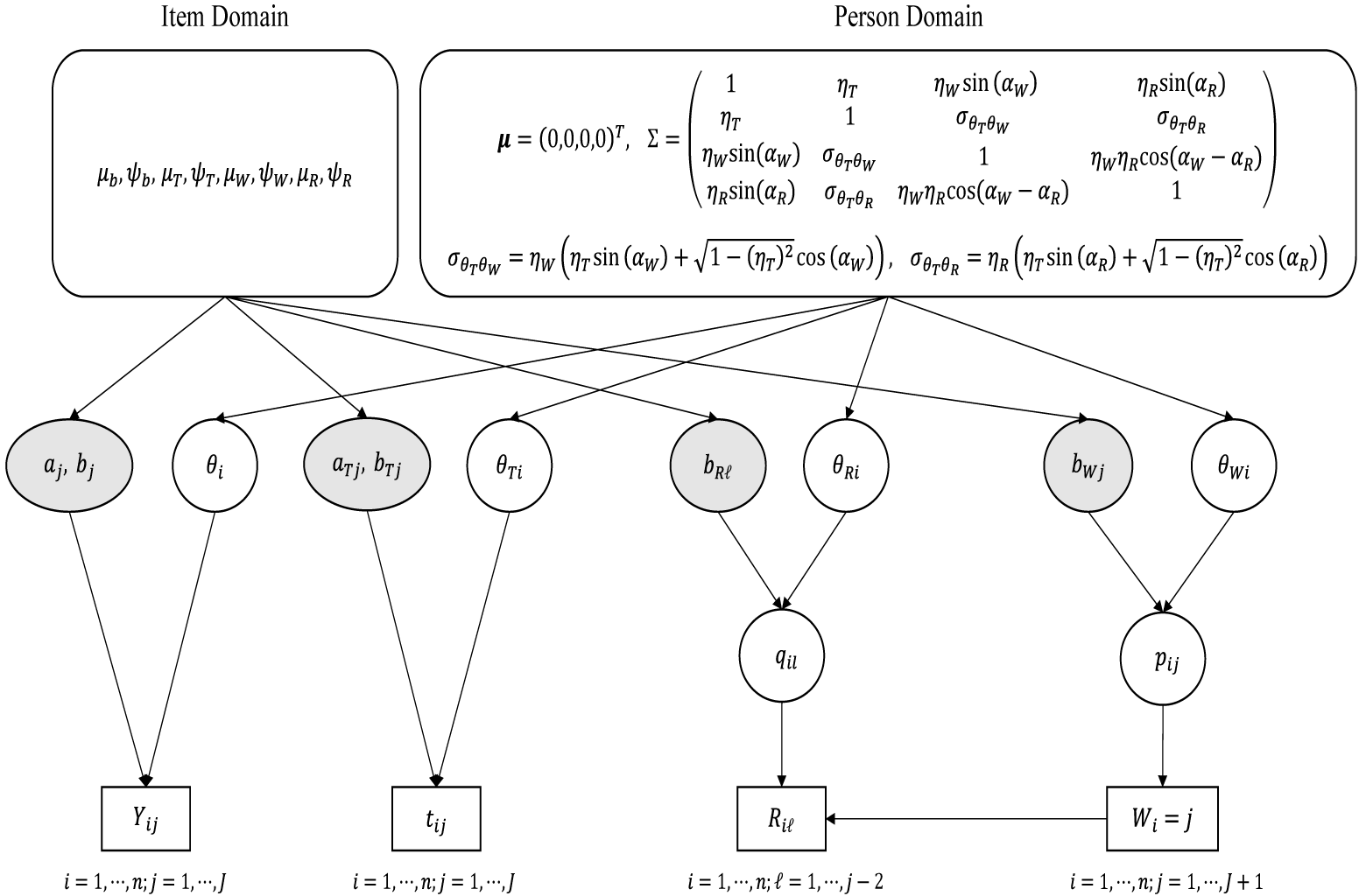
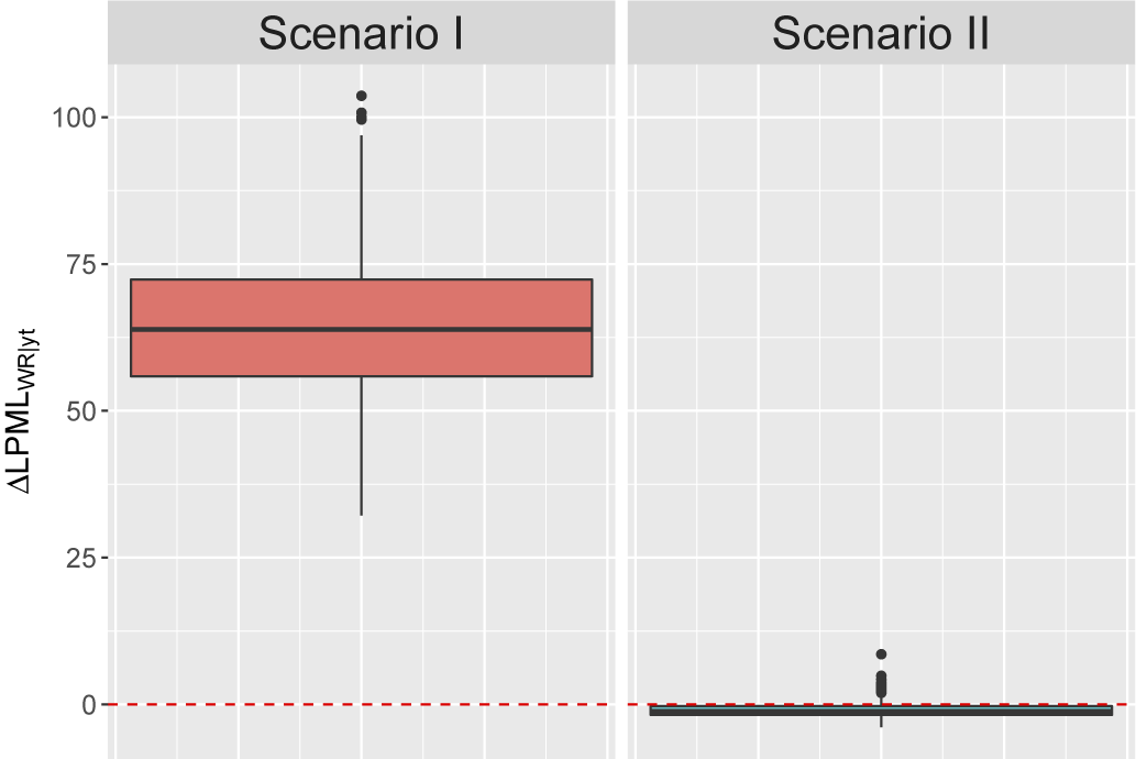

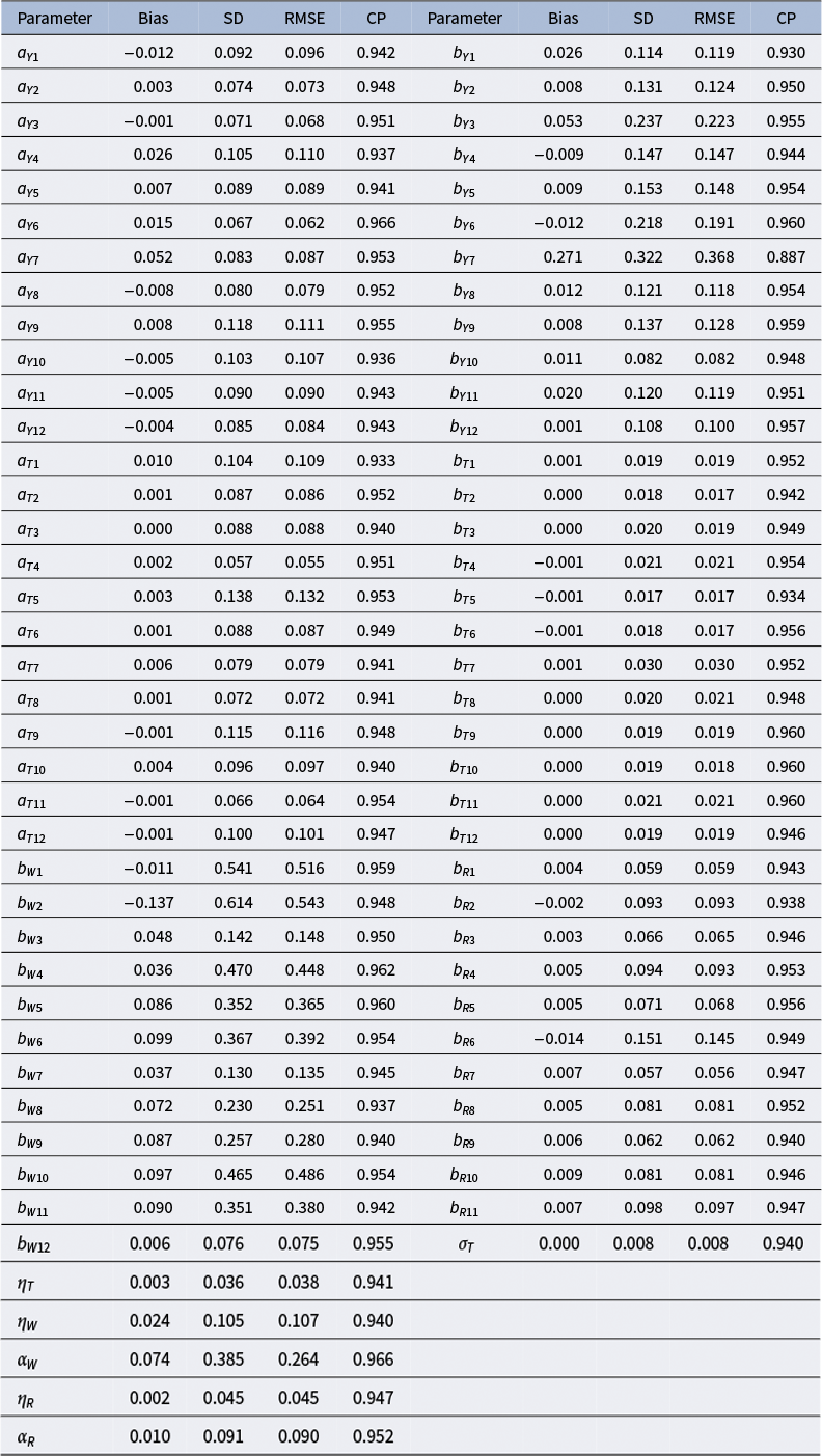


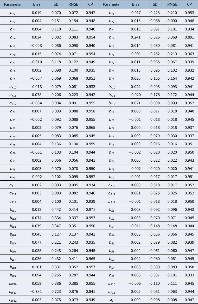


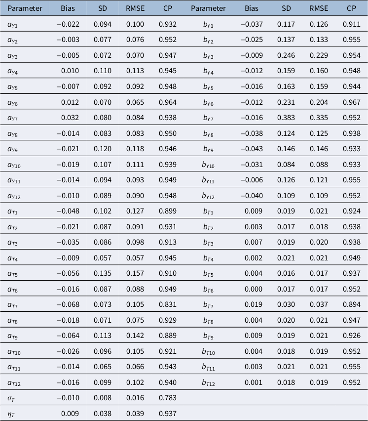


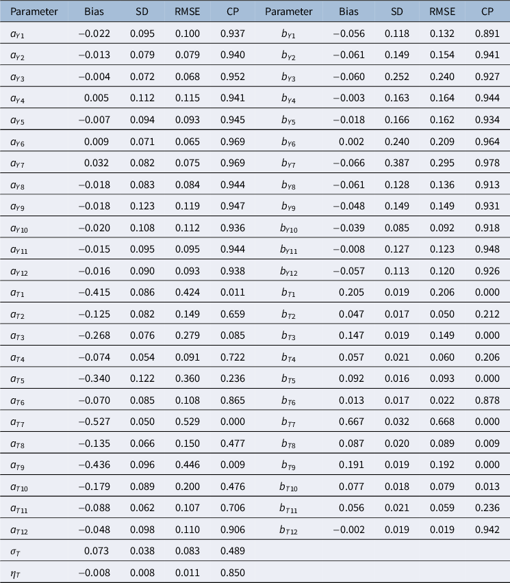


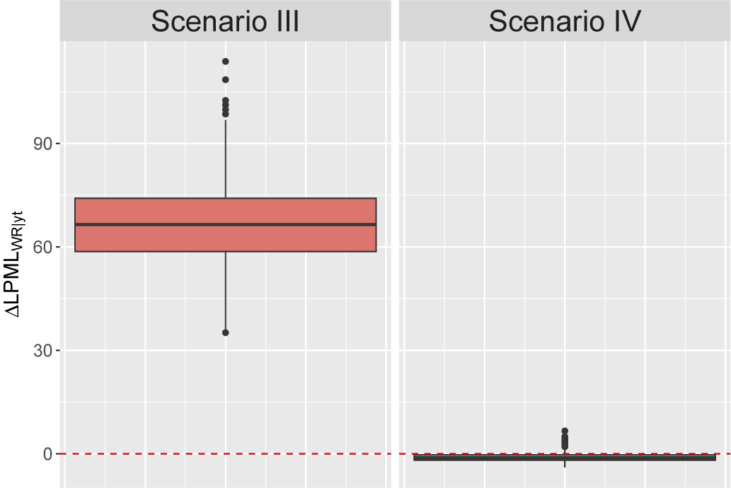

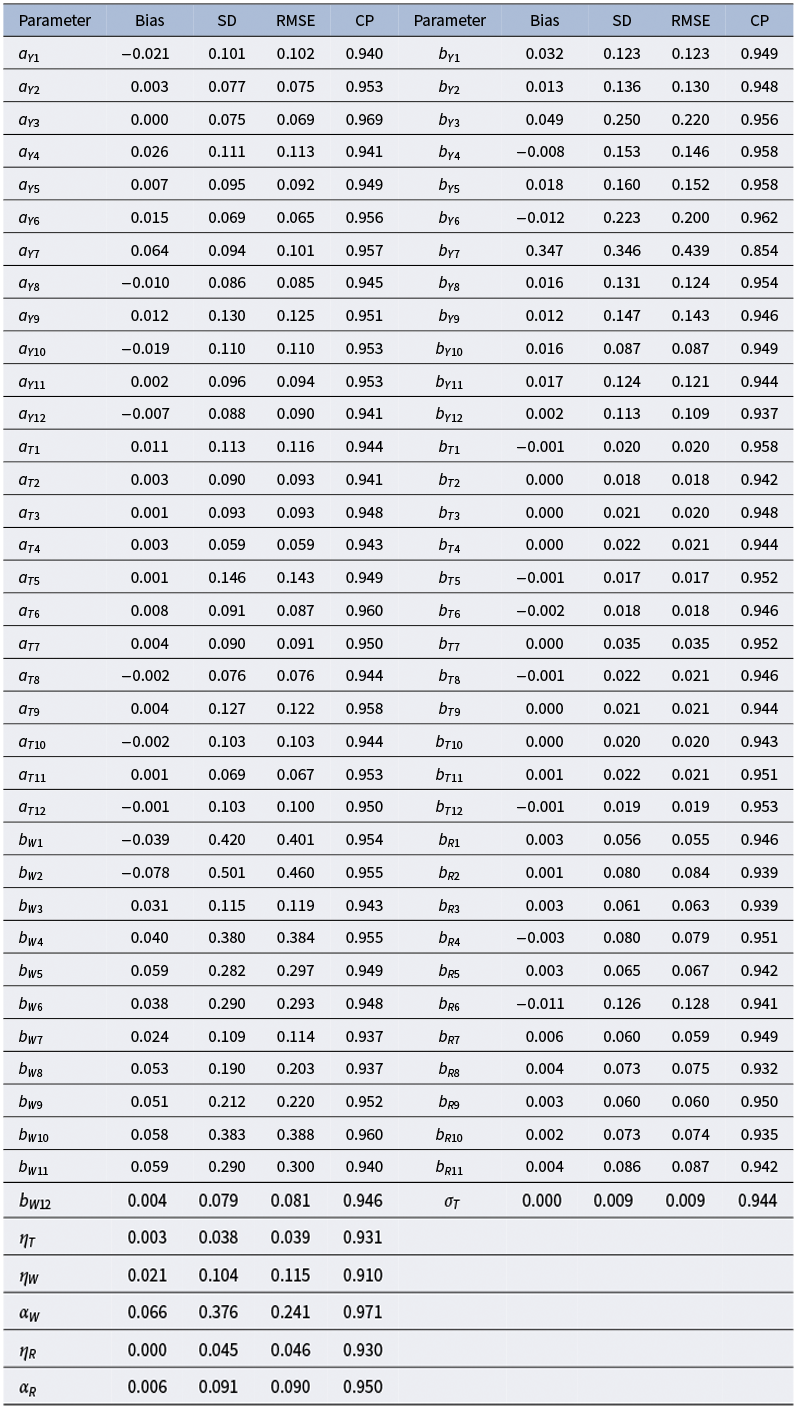


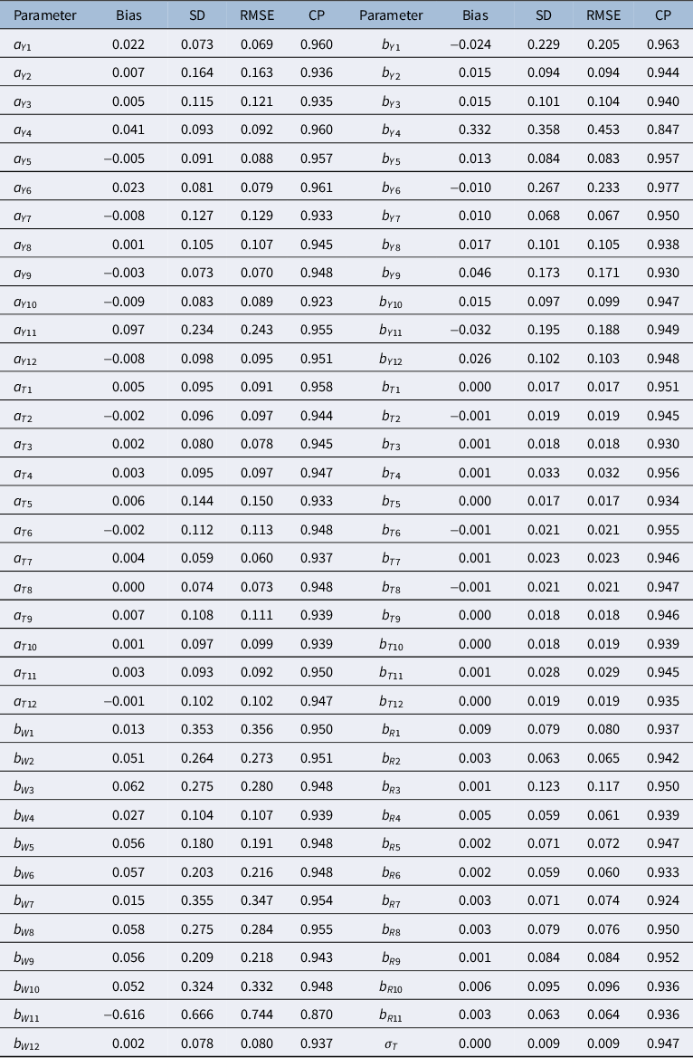


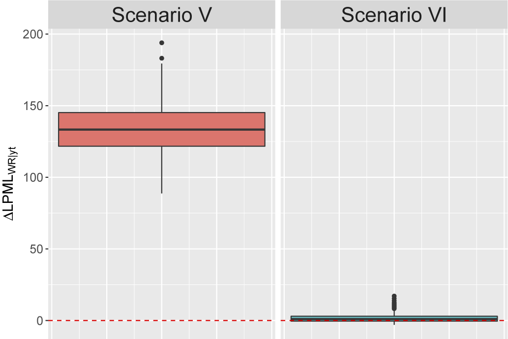


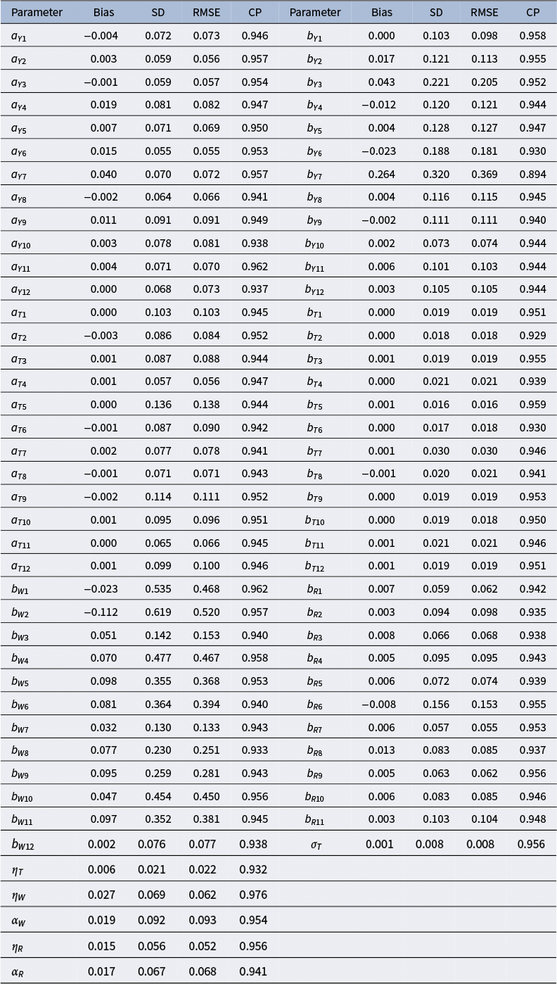


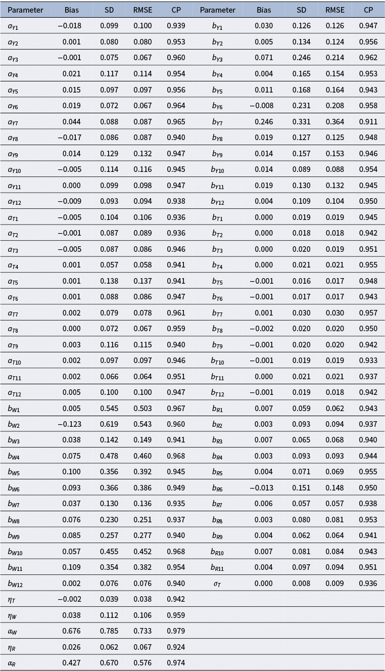


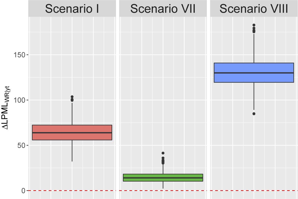


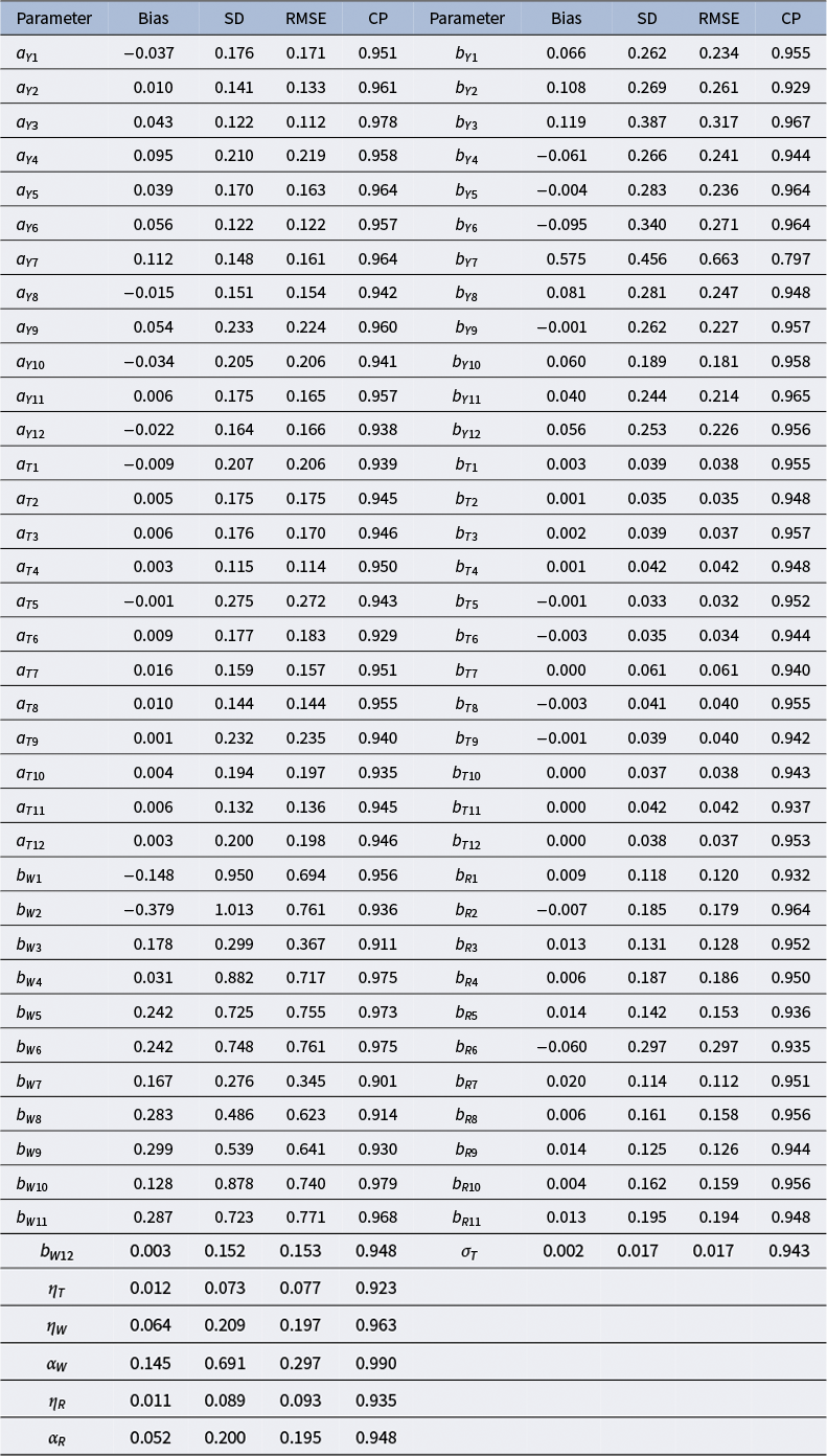


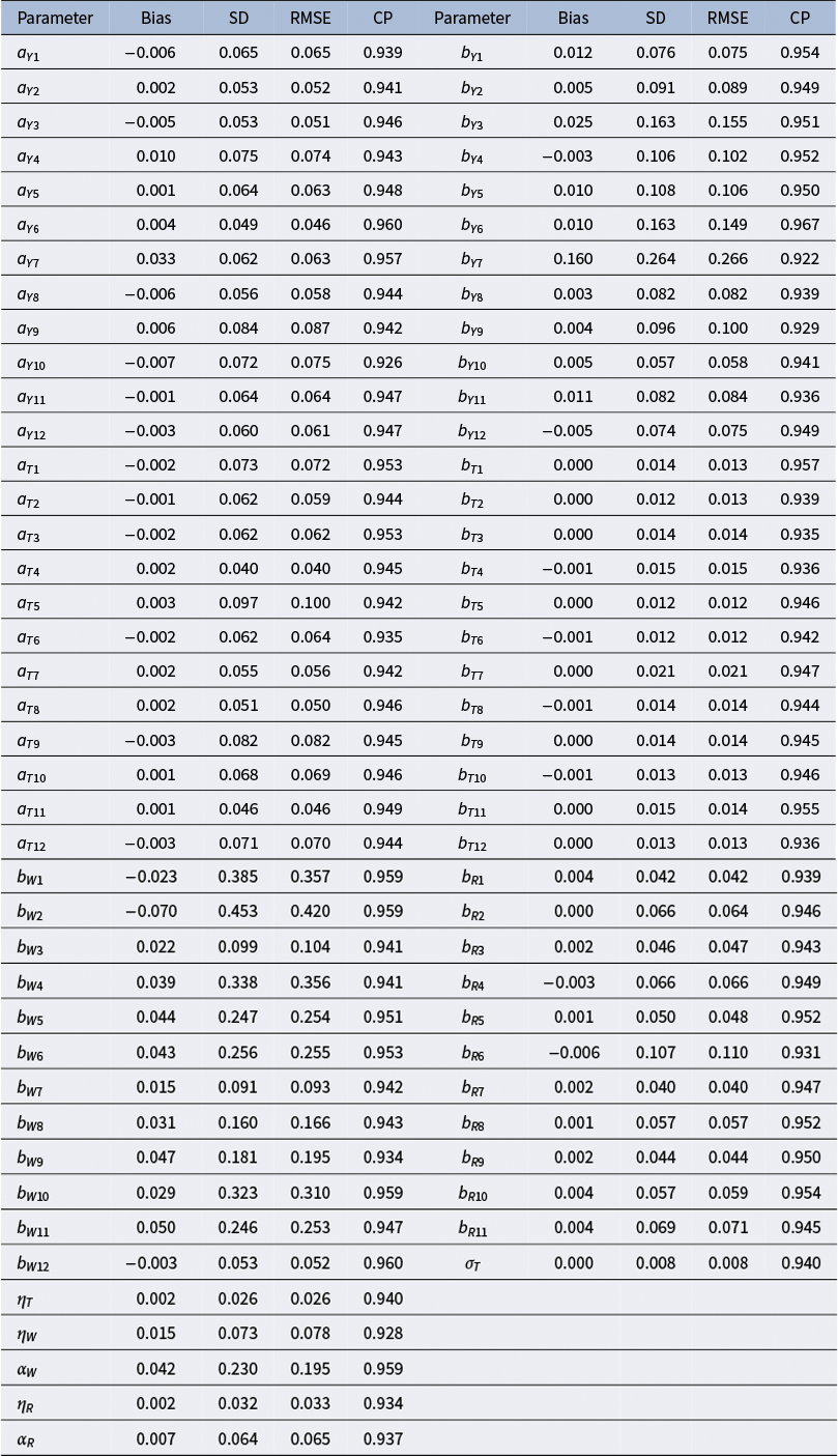


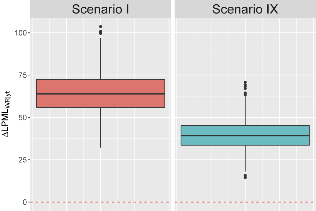

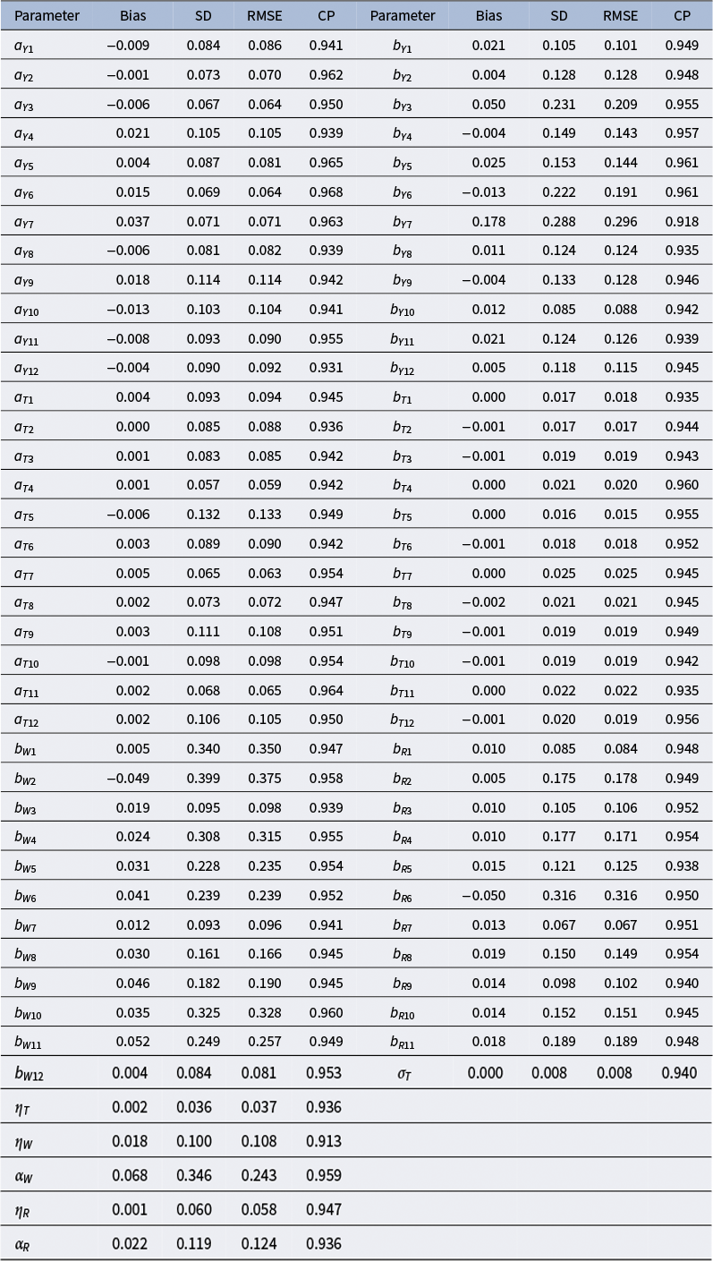


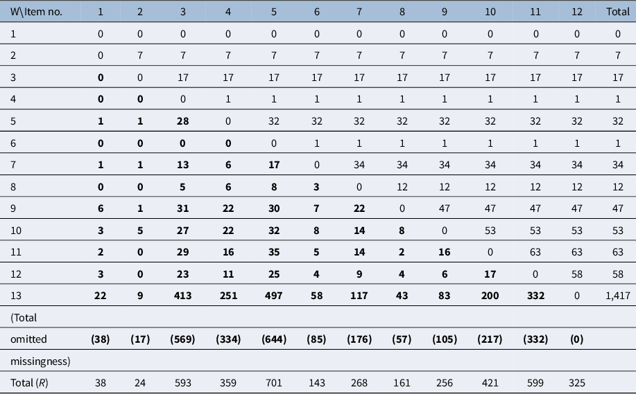

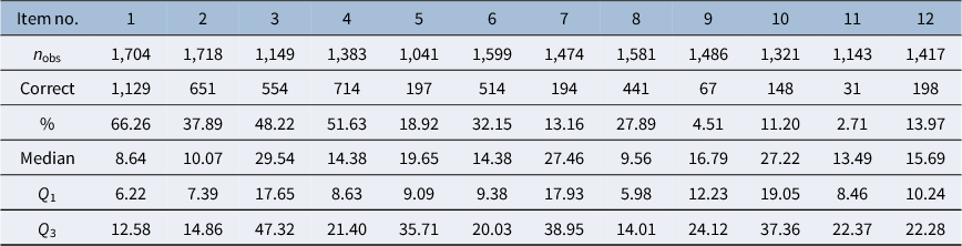


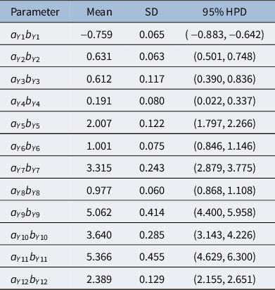
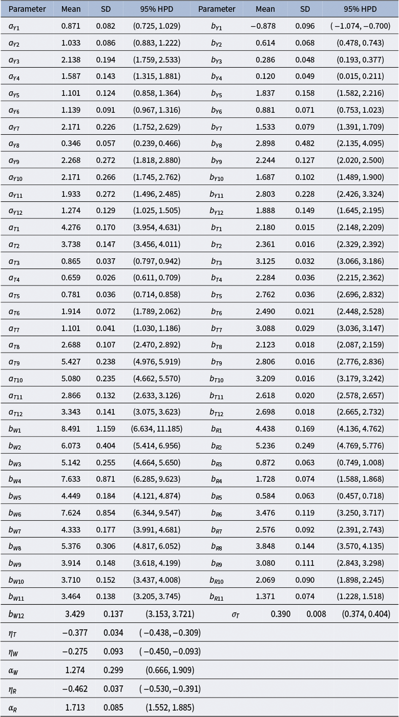
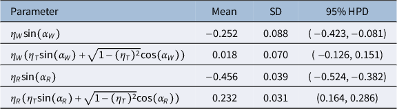
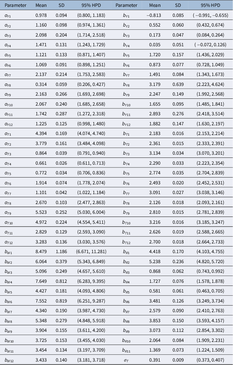
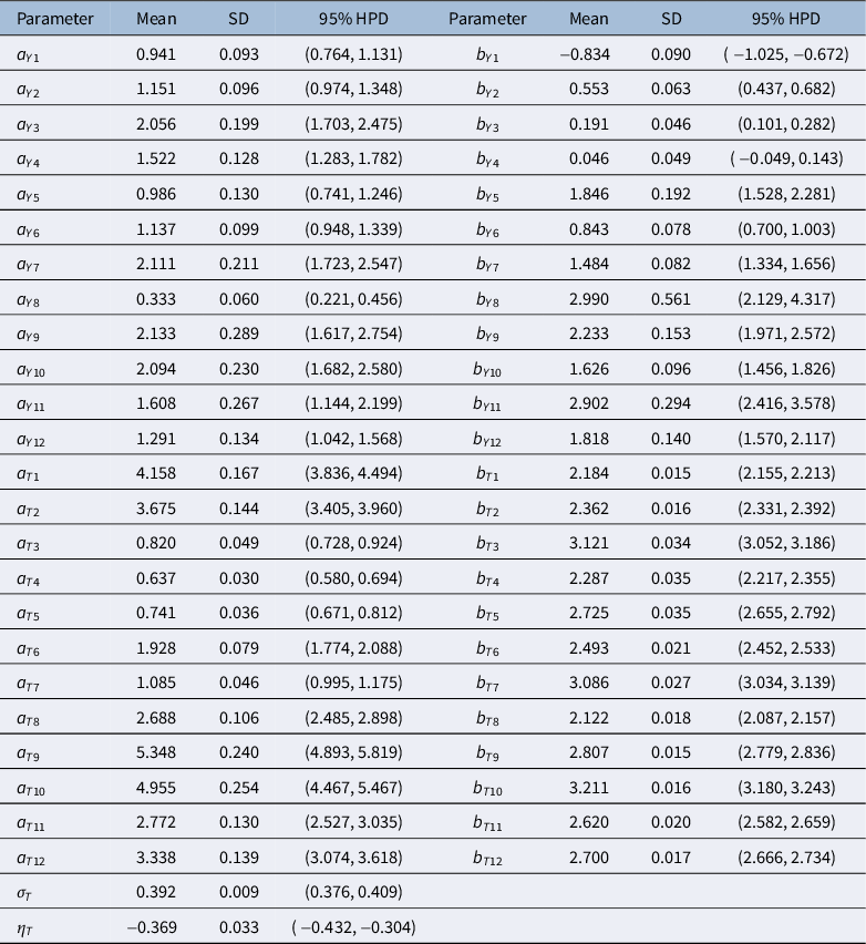
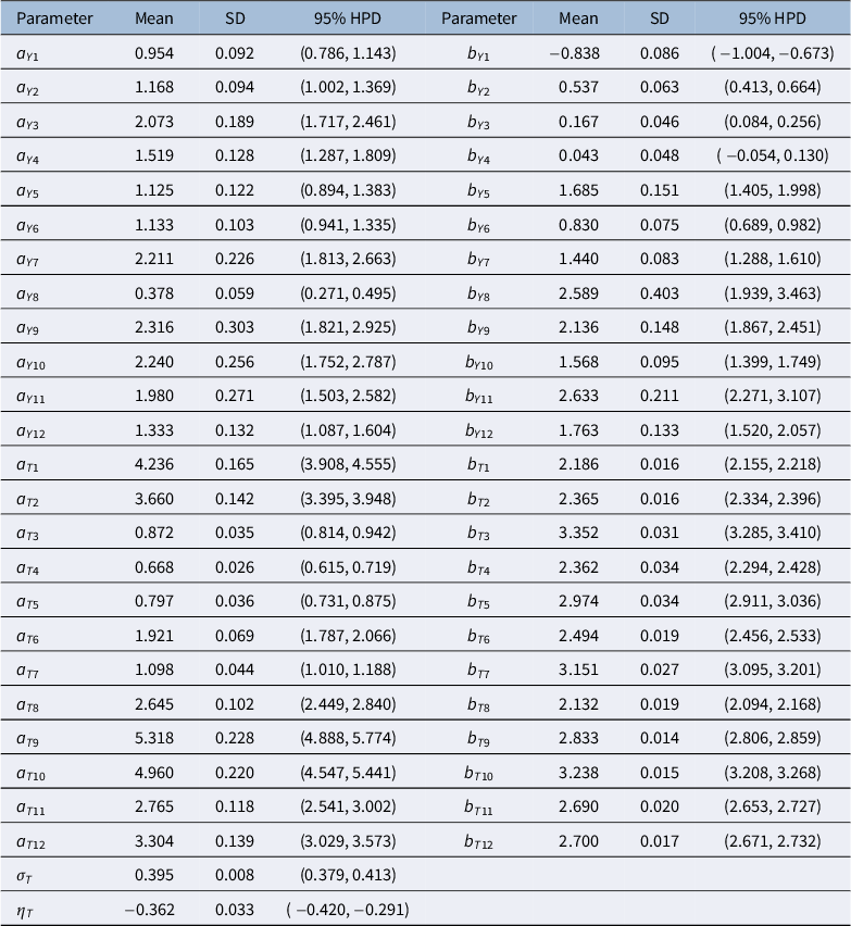
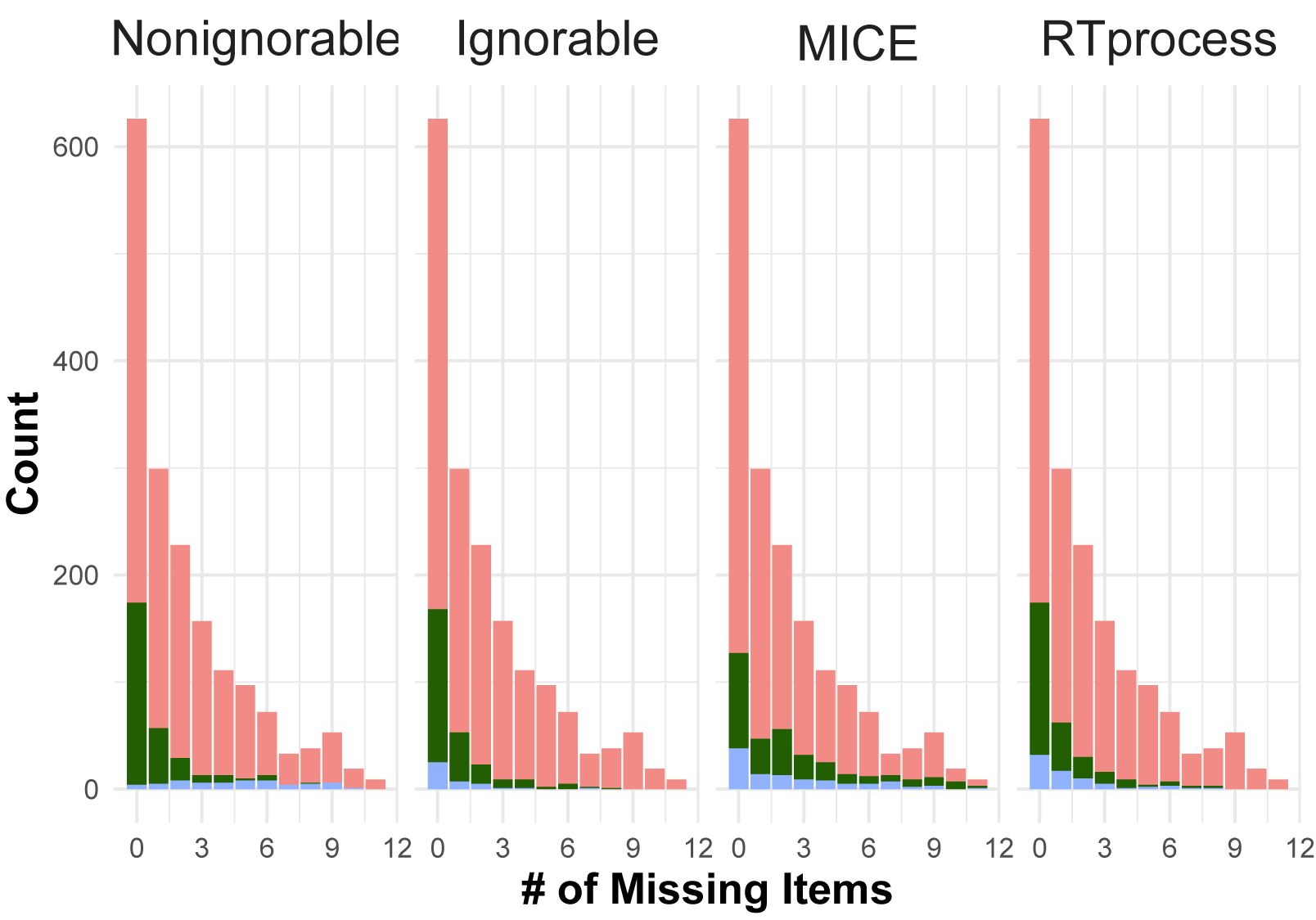


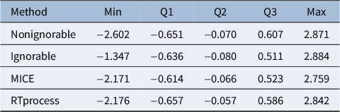
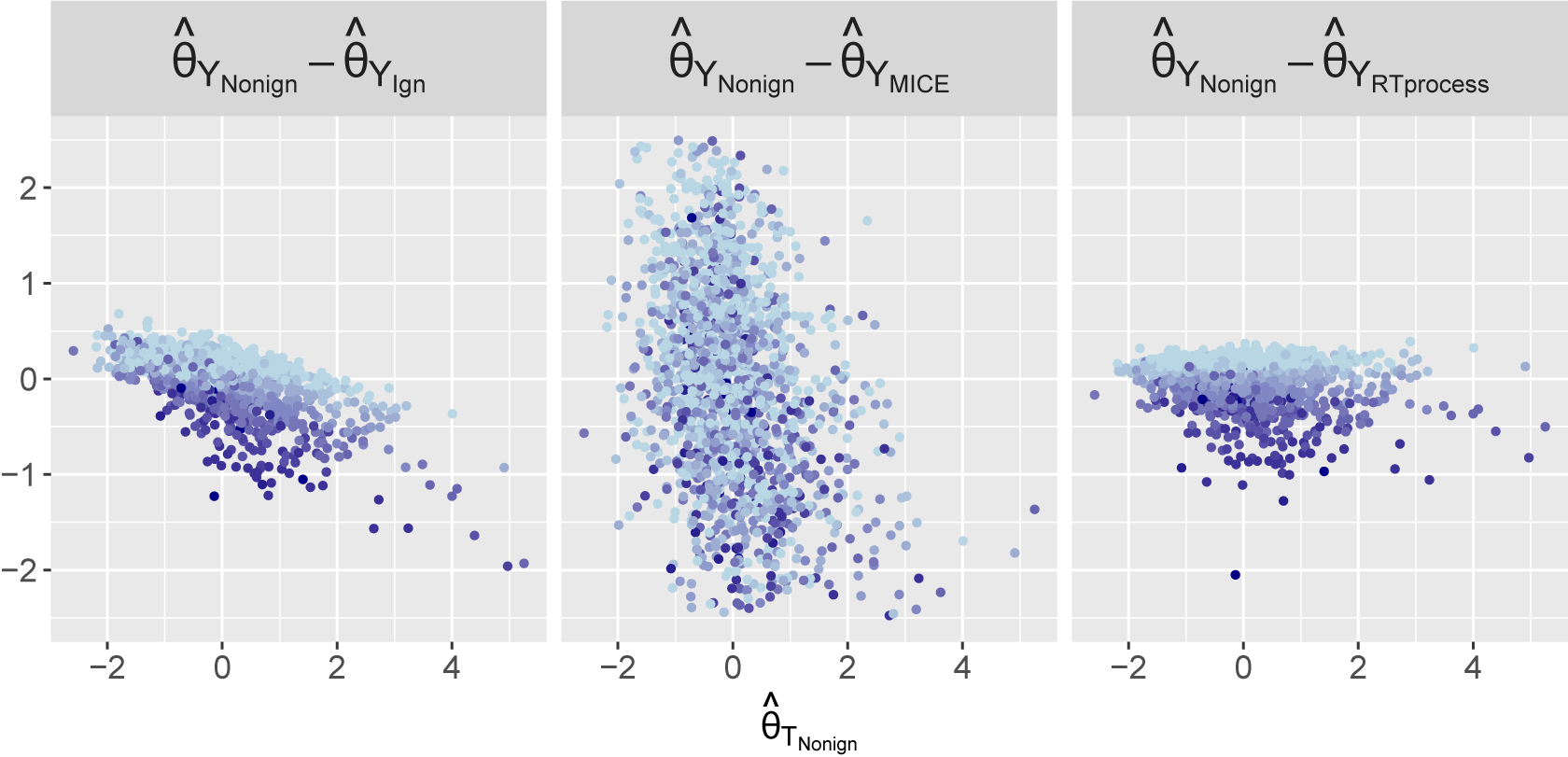


 Open access

