2.1 Cybersecurity simulations and games

Many approaches have been taken to simulating APT threats, which often take the form of a two-player game. In Zhu and Rass (Reference Zhu and Rass2018), a multi-stage game is proposed with different action and rewards in each phase. In Luh et al. (Reference Luh, Temper, Tjoa, Schrittwieser and Janicke2019), a physical game is used with two stages. Many similarities exist in these games, namely they tend to involve two players (an attacker and a defender) alternating moves, discrete action spaces, and asymmetric information between attacker and defender. Other cybersecurity simulation and game approaches include (Rush et al., Reference Rush, Tauritz and Kent2015; Liu et al., Reference Liu, Yasin Chouhan, Li, Fatima and Wang2018; Yang et al., Reference Yang, Pengdeng, Zhang, Yang, Xiang and Zhou2018; Baillie et al., Reference Baillie, Standen, Schwartz, Docking, Bowman and Kim2020; Molina-Markham et al., Reference Molina-Markham, Winder and Ridley2021; Reinstadler, Reference Reinstadler2021).

CyberBattleSim contains many of these elements, and is also implemented using OpenAI Gym, making it well-suited for reinforcement learning (Brockman et al., Reference Brockman, Cheung, Pettersson, Schneider, Schulman, Tang and Zaremba2016). It also contains additional complexity compared to these environments (Team, Reference Team2021) and is one of the few that has been publicly released. Deceptive elements, including honeypots and decoys, were incorporated into CyberBattleSim in Walter et al. (Reference Walter, Ferguson-Walter and Ridley2021).

Some of these authors have implemented various policy search algorithms in order to train automated attackers and defenders in these environments, such as AI planning or deep reinforcement learning. We describe these methods below.

2.2 Algorithms for training

We describe AI Planning using Monte Carlo Tree Search (MCTS), Deep Reinforcement Learning (DRL) work related to cybersecurity games, and Evolutionary Strategies (ES).

AI Planning Planning is a long established field of AI research focused on training agents to make optimal decisions (Jiménez et al., Reference Jiménez, De La Rosa, Fernández, Fernández and Borrajo2012). Planning has been successfully applied in reinforcement learning domains (Partalas et al., Reference Partalas, Vrakas and Vlahavas2012). Recently, AlphaZero (Silver et al., Reference Silver, Hubert, Schrittwieser, Antonoglou, Lai, Guez, Lanctot, Sifre, Kumaran, Graepel, Lillicrap, Simonyan and Hassabis2018) combined planning with deep learning, and was able to successfully master several complex board games. In combination with evolutionary algorithms, planning is used to solve RL environments in Olesen et al. (Reference Olesen, Nguyen, Palm, Risi, Castillo and Jiménez Laredo2021). Planning has seen some use in cybersecurity. In the domain of automated penetration testing, planning has been used for attack graph discovery (Applebaum et al., Reference Applebaum, Miller, Strom, Korban and Wolf2016; Backes et al., Reference Backes, Hoffmann, Künnemann, Speicher and Steinmetz2017; Falco et al., Reference Falco, Viswanathan, Caldera and Shrobe2018; Reinstadler, Reference Reinstadler2021). However, planning has not been used extensively to train agents within cybersecurity platforms.

Deep Reinforcement Learning (DRL) Deep reinforcement learning (DRL) is a subfield of RL focusing on using deep neural networks to represent a policy and gradient-based ML methods to train the network parameters. Interest in DRL has exploded in recent years due to breakthrough papers such as Mnih et al. (Reference Mnih, Kavukcuoglu, Silver, Rusu, Veness, Bellemare, Graves, Riedmiller, Fidjeland, Ostrovski, Petersen, Beattie, Sadik, Antonoglou, King, Kumaran, Wierstra, Legg and Hassabis2015) and Lillicrap et al. (Reference Lillicrap, Hunt, Pritzel, Heess, Erez, Tassa, Silver and Wierstra2016). For a survey of DRL methods, see Arulkumaran et al. (Reference Arulkumaran, Deisenroth, Brundage and Bharath2017). DRL has also been applied in cybersecurity domains, for a survey see Nguyen and Reddi (Reference Nguyen and Reddi2021). However, most of these environments involve a small number of actions for the attackers, and only some involve coevolving attackers and defenders together. In the initial release of CyberBattleSim (Team, Reference Team2021), automated attackers were trained using Q-learning methods without any defenders. Additionally, the action space was simplified to reduce complexity. We develop a neural network architecture that allows attackers to select complex actions within the CyberBattleSim environment and train attackers and defenders together. Our approach is similar to the action selection process in AlphaStar (Vinyals et al., Reference Vinyals, Babuschkin, Czarnecki, Mathieu, Dudzik, Chung, Choi, Powell, Ewalds, Georgiev, Oh, Horgan, Kroiss, Danihelka, Huang, Sifre, Cai, Agapiou, Jaderberg, Vezhnevets, Leblond, Pohlen, Dalibard, Budden, Sulsky, Molloy, Paine, Gulcehre, Wang, Pfaff, Wu, Ring, Yogatama, Wünsch, McKinney, Smith, Schaul, Lillicrap, Kavukcuoglu, Hassabis, Apps and Silver2019), which was designed to select complex actions in the video game StarCraft.

Evolutionary Strategies Evolutionary strategies (ES) are a subset of evolutionary algorithms, a broad class of population-based optimization algorithms modeled on genetic evolution (Goldberg, Reference Goldberg1989). ES are commonly used with a population (sample) size of one, although the Cross-Entropy method uses a sample size greater than one. For simulations where a solution has to be competed to determine its fitness, all solutions in a sample can be competed with all adversaries, resulting in a quadratic number of competitions. To reduce the number of competitions to polynomial complexity, small sample subsets can be formed and competition can be restricted to a subset. We call this round-robin play. Evolutionary strategies (ES) have seen heightened interest in RL environments due to the success of authors such as Salimans et al. (Reference Salimans, Ho, Chen and Sutskever2017), where ES are applied to MuJoCo and Atari RL environments and shown to outperform some deep learning algorithms. Some authors have also combined ES with DRL methods; in Lee et al. (Reference Lee, Lee, Shin, Kweon, Larochelle, Ranzato, Hadsell, Balcan and Lin2020), an asynchronous framework is proposed and shown to outperform pure DRL methods in MuJoCo. DRL is also combined with population-based and exploration methods from evolutionary computation in Prince et al. (Reference Prince, McGehee, Tauritz, Castillo and Jiménez Laredo2021). However, to our best knowledge there are few precedents that apply ES to cybersecurity simulations.

Coevolution, broadly speaking, refers to environments where agents are trained with different (possibly competing) objective functions. Evolutionary algorithms have long been applied to coevolutionary environments, see Potter and Jong (Reference Potter and Jong2000) for instance. They have also been used in predator-prey environments with two opposing agents (Simione & Nolfi, Reference Simione and Nolfi2017; Harris & Tauritz, Reference Harris and Tauritz2021). ES have also been applied to coevolution in two-player board games; for example in Schaul & Schmidhuber (Reference Schaul and Schmidhuber2008), where they were able to learn some complex strategies. Planning with tree search (Liu et al., Reference Liu, Pérez-Liébana and Lucas2016) and deep reinforcement learning (Klijn & Eiben, Reference Klijn and Eiben2021) have also been utilized in coevolutionary RL environments. Finally, competitive fitness functions for one population were investigated in Panait and Luke (Reference Panait and Luke2002), where a one-population fitness function is optimized using a round-robin method.

3.1 Connect 4

Connect 4 is a simple two-player zero-sum game which has previously been used for reinforcement learning investigations (Allis, Reference Allis1988). Connect 4 is played on an upright board with six rows and seven columns. Players alternate dropping tokens into a column until one of them wins by having a line of four tokens vertically, horizontally or diagonally. If all seven columns are filled without a winner, then the game ends in a tie. While the game is simple enough to have been solved, perfect play requires complex strategies (Bräm et al., Reference Bräm, Brunner, Richter, Wattenhofer, Brefeld, Fromont, Hotho, Knobbe, Maathuis and Robardet2020). Note, players in Connect 4 are neither attacker or defender, instead players are evaluated based on who plays first and second.

3.2 Simple Network APT (SNAPT)

PenQuest (Luh et al., Reference Luh, Temper, Tjoa, Schrittwieser and Janicke2019) provides an APT threat model designed to simulate attacker/defender behavior in an abstract network with imperfect information and is implemented as a board game. We design a simpler APT threat model inspired by PenQuest to evaluate our algorithms. It is called Simple Network Advanced Persistent Threat (SNAPT). SNAPT is implemented as a game between ‘attacker’ and ‘defender’, who alternate taking actions. The attacker starts and the game ends after a certain number of moves by each player. Note, the attacker’s actions mimic two cyberattack campaign tactics listed in the MITRE ATT&CK Matrix (Corporation, n.d.a). The change in the device’s security state through exploits mimics the tactic of privilege escalation. Attacking of adjacent nodes mimics the tactic of lateral movement. The defender mimics two defensive approaches of the MITRE Engage (Corporation, n.d. b) cyberdefense framework for adversary engagement operations. The detect action mimics the defensive goal of exposing an adversary through the approach of detection. The secure device action mimics the defensive goal of affecting the adversary with the approach of disrupting the adversaries operation.

SNAPT States SNAPT models a network as an unweighted graph where nodes are individual devices. Edges indicate that two devices are connected in some way (e.g. by a router). Aside from its connectivity, each device has three properties: its security state s, which is either ‘secure (S)’, ‘vulnerable (V)’, or ‘compromised (C)’; its value, which is its worth to an attacker; and its vulnerability probability, which is the likelihood that an exploit will succeed if used against it. We represent these properties as a tuple (s, v, p), where $s \in \{S, V, C\}$ is the security state, and $v,p \in[0,1]$ are the value and vulnerability probability, respectively. Figure 1 shows an example SNAPT network.

Figure 1.

The SNAPT setup used for training with three nodes. Each node contains the triple of data (s, v, p) equal to the security state(s), value(v) and exploit probability(p).

Figure 2.

The network topology of a CyberBattleSim environment. Nodes represent devices and edges represent potential exploits sourced at the tail of the arrow and targeted at the head. The label of each node is its type. At the start of the simulation, the attacker has control of only the ‘Start’ node and needs to control the ‘Goal’ node in order to receive the full reward.

The SNAPT game begins with the one device in the network, representing a device connected to the Internet, being in a ‘vulnerable’ state, and all other devices being ‘secure’. The attacker and defender have asymmetric information on the status of the network. The attacker knows the security state s of each device, the defender knows the exploit probability $p_e$ of each device, and both players know the value v of each device.

SNAPT actions During an attacker’s turn, they select a device to target with an exploit. Attackers may only target devices which are in a vulnerable state, or which are connected to a device in a vulnerable state. Exploits succeed with a probability equal to the device’s vulnerability probability and raise the security state of a device from secure to vulnerable or vulnerable to compromised if they succeed.

The defender can take two kinds of mitigation actions: detecting exploits and securing devices. Detection actions are only effective against devices which were successfully compromised in the previous turn. If the defender targets a detection action against a device which was not compromised in the previous turn, the action immediately fails and nothing happens. Otherwise, the action succeeds with probability $p_d$ . If the action succeeds, the security state of the device is reduced. If the action does not succeed, the network is left unchanged.

Moreover, the defenders have no knowledge of the security state of each device, so they have to ‘guess’ which device the attacker is likely to have targeted when using detection. If the defender targets a securing action at a certain device, the exploit probability of that device is reduced, making an attacker’s exploit less likely to succeed by a fixed value $\delta_s$ . However, defenders have limited number of resources to secure a device and may only secure a specific device a maximum of three times. Furthermore, the attackers have no knowledge of the exploit probabilities of devices, so they are unaware if a device has been secured.

SNAPT rewards At the end of the game, the attacker receives a reward equal to sum of the value of all the devices in a ‘compromised’ state. Given a network with devices $(d_1, d_2, \ldots, d_n)$ , with device $d_i$ having properties $(s_i, v_i, p_i)$ , the reward R is given by

(1) \begin{align} R =& \sum_{1\le i \le n,\ s_i = C} v_i\end{align}

If $R \ge 1$ , the attacker wins, otherwise the defender wins.

3.3 CyberBattleSim

CyberBattleSim (Team, Reference Team2021) is a network simulation in which an automated attacker attempts to take control of a network, and an automated defender tries to deter the attacker. The network is represented as a directed graph, with each node representing a device and each edge directed from node X to node Y representing an exploit sourced at device X targeting device Y, for a concrete CyberBattleSim network example see Figure 2. Each machine has a specific set of vulnerabilities which may be exploited, as well as a specific value representing its importance to the attacker and defender.

CyberBattleSim is implemented as a reinforcement learning environment, where at a given time t an agent receives an observation of the state $s_t$ , takes an action $a_t$ and then receives a reward $r_{t+1}$ as well as the observation for the next state $s_{t+1}$ . The agent then takes an action $a_{t+1}$ and the cycle continues until either a terminal state is reached or the maximum number of time steps is surpassed.

CyberBattleSim States In our CyberBattleSim environment, there are two agents, the attacker and the defender, which receive different observations at each time step in order to model the asynchronous information of a real network. Additionally, the observation given to the attacker is dependent on how much of the network the attacker has discovered and controls. For instance, the attacker receives no information on nodes it has not discovered. The specifics on the information given to the attacker and defender can be found in Appendix C.

CyberBattleSim Actions The attacker and defender also take different actions representative of their different roles. The attacker can take three kinds of actions at each time step: local exploits (e.g. privilege escalation techniques), remote exploits (e.g. lateral movement techniques), and connections (e.g. lateral movement techniques). These actions are abstracted as tuples: $(\alpha, T)$ for local exploits, $(\alpha, T,S)$ for remote exploits, and $(\alpha, T, S, C)$ for connections, where $\alpha$ is the action type, T is the target node, S is the source node, and C is the credential used. Note that only $\alpha$ and T are necessary information for every type of action, while S is only necessary for remote exploits and connections and C is only needed for connections. The defender recovers against the attacker by ‘reimaging’ nodes, and only needs to choose a node T to target during the reimaging process. When a node is selected to be reimaged, it goes into an ‘offline’ state for a fixed number of time steps, making it unavailable to exploits. After reimaging, nodes are returned to their original state, without any exploits used against them. Only certain nodes are available for reimaging (representing non-critical infrastructure in a network) and the defender may only reimage a node every $t_I$ time steps. The defender may also choose to leave the network unchanged. The specifics on the information given to the attacker and defender can be found in Appendix C.

CyberBattleSim Rewards The attacker earns rewards for successfully using exploits against nodes in the network, and loses rewards when an exploited node is reimaged. The defender’s reward is the negative of the attacker’s reward. The reward given by reimaging a node is equal to the negative sum of the rewards of all exploits used against that node since its last reimaging. For instance, if an attacker has used 2 exploits against a node X for a total reward of 100, the attacker will be given a reward of $-100$ when the node is reimaged and the defender will be given a reward of 100. In the initial release of CyberBattleSim, no rewards were given out due to reimaging, and we make this modification in order to give the defender greater influence over the rewards in the network. Denote the attacker’s reward at time t by $r^A_t$ and the defender’s reward by $r^D_t$ . As the defender only takes an action every $t_I$ time steps, $r^D_t = 0$ if $t \not\equiv 0(\textrm{mod} \ t_I)$ . If $t \equiv 0 (\textrm{mod} \ t_I)$ , then the reward given to the defender is the negative of the attacker’s reward from the previous $t_I$ time steps:

\begin{align*} r^D_{t} = -\!\!\sum_{i = t - t_I + 1}^t r^A_t \end{align*}

The simulation ends when the attacker reaches a winning state or the current time t is greater than some predefined threshold $t_{\textit{max}}$ . Winning states are those where the attacker has complete control of the network or the number of nodes in an ‘offline’ state due to reimaging exceeds a predefined threshold, in which case a reward is given to the attacker and a penalty given to the defender. Thus, the defender’s goal is to reimage nodes strategically to deter the attacker while making sure that enough of the network is online so that the simulation does not end.

4.1 Neural network architectures

Connect 4 We represent each player’s policy with an actor-critic approach which uses two feed-forward NNs with two hidden layers. They map state observation vectors to action probabilities and values. The value $v_t$ of a state is the expected reward of that state, see Figure 3.

Figure 3.

The neural network (NN) architecture used for the defender. When choosing an action, the actor/policy NN picks a node T to reimage or to leave the network unchanged (this can be seen as picking a ‘null’ node). The value is chosen separately by the critic/value NN.

SNAPT For SNAPT the Defender’s policy and value neural networks are two feed-forward NNs with two hidden layers, similar to Connect 4, see Figure 3.

CyberBattleSim In CyberBattleSim, due to a more complex action space, Attackers use a multi-stage NN similar to the approach introduced in Metz et al. (Reference Metz, Ibarz, Jaitly and Davidson2017) and implemented in Vinyals et al. (Reference Vinyals, Babuschkin, Czarnecki, Mathieu, Dudzik, Chung, Choi, Powell, Ewalds, Georgiev, Oh, Horgan, Kroiss, Danihelka, Huang, Sifre, Cai, Agapiou, Jaderberg, Vezhnevets, Leblond, Pohlen, Dalibard, Budden, Sulsky, Molloy, Paine, Gulcehre, Wang, Pfaff, Wu, Ring, Yogatama, Wünsch, McKinney, Smith, Schaul, Lillicrap, Kavukcuoglu, Hassabis, Apps and Silver2019). Each stage is a feed-forward neural network with two hidden layers. The policy network first passes the state $s^A_t$ into the ‘attack type neural network’ which returns a probability vector for the attack type $\alpha$ (see Section 3.3). Once $\alpha$ is chosen using the given probabilities, $\alpha$ is concatenated with $s^A_t$ and passed into the ‘target neural network’ which returns a probability vector for the target node T. The order of these steps: Type before Target, can be switched to Target before Type. We compare the two orderings in our experiments.

Should a source decision be needed, T is concatenated onto the state vector (along with $\alpha$ ) and passed into the ‘source neural network’. If the action type is ‘connection’, then finally $\alpha$ , T, and S are concatenated onto $s^A_t$ and passed into the ‘credential neural network’.

This approach decomposes the attacker’s action selection into at most four steps, each with a significantly smaller output vector. A summary of the attacker neural network design is shown in Figure 4.

Figure 4.

The multi-stage neural network (NN) architecture used for the attacker. When choosing an action, each element of the tuple is selected individually and passed onto the next stage of the actor/policy neural network. The ordering of the Type NN and Target NN may be swapped, and the Source NN and Credential NN are only used for certain action types. The value is chosen separately by the critic/value NN.

4.2 Policy learning algorithms

We characterize the different algorithms we use to train our policies in Table 1. The algorithms vary in parameter updates during training, the number of neural network samples used, and the use of tree search.

Table 1.

Overview of training methods. The methods are chosen based on how they update the neural network. The training choices are gradient descent and/or weighted average, the number of samples (#Samples) used, and if tree search is used

Figure 5.

The iterative process used for evolutionary strategies (ES). At iteration t, a set of samples is taken from the distribution $(\mu_t, \sigma_t)$ . These samples are then evaluated by executing episodes of CyberBattleSim. Sample performance is determined by average reward from these episodes. The distribution is then updated towards the better performing samples. The process then begins again with the new distribution $(\mu_{t+1}, \sigma_{t+1})$ .

4.2.2 Evolutionary Strategies (ES)

Evolutionary strategies (ES) are a class of optimization algorithms based on biological evolution (Rechenberg, Reference Rechenberg and Bergmann1989). A high-level overview of ES algorithms can be found in Figure 5. We utilize three ES algorithms: $(1+1)$ -ES (Droste et al., Reference Droste, Jansen and Wegener2002), fitness-based ES (Lee et al., Reference Lee, Lee, Shin, Kweon, Larochelle, Ranzato, Hadsell, Balcan and Lin2020), and the cross-entropy method (CEM) (Hansen, Reference Hansen2016). All three rely on iterating a multi-variate Gaussian distribution of the parameters of the attacker and defender network. The distributions at time t are given by $(\mu^A_t, \sigma^A_t)$ and $(\mu^D_t,\sigma^D_t)$ for the attacker and defender, respectively, where $\mu_t$ is the mean and $\sigma_t$ is the covariance matrix. We will sometimes omit the superscript A or D in writing operations which are performed on both distributions. In order to reduce computational complexity, we constrain $\sigma_t$ to be diagonal as in Pourchot and Sigaud (Reference Pourchot and Sigaud2018). Thus $\sigma_t$ can be interpreted as a vector, and we write $\sigma_t^2$ to mean the square of each element in $\sigma_t$ . Our ES methodology is derived from Lee et al. (Reference Lee, Lee, Shin, Kweon, Larochelle, Ranzato, Hadsell, Balcan and Lin2020).

(1+1)-ES (Droste et al., Reference Droste, Jansen and Wegener2002) In $(1+1)$ -ES, a single-sample $z^A$ and $z^D$ is taken from the distributions $(\mu^A_t, \sigma^A_t)$ and $(\mu^D_t,\sigma^D_t)$ . A fixed number $G_{(1+1)}$ of simulations are rolled out for each of the four attacker-defender pairings $(\mu^A_t, \mu^D_t),(\mu^A_t, z^D), (z^A, \mu^D_t), (z^A, z^D)$ and the average reward for each agent over the simulations is calculated. In this way the mean and sample face each opponent the same number of times, allowing for a more balanced evaluation. We are also able to evaluate attackers and defenders simultaneously this way, reducing the number of competitions executed in each training step. If the sample z outperforms $\mu_t$ (i.e. it has a higher average reward), the distribution is updated by

(2) \begin{align} \mu_{t+1} = z \quad & \mbox{and} \quad \sigma^2_{t+1} = (\mu_t - z ) ^2\end{align}

In order to guarantee convergence, we also introduce an update to $\sigma_t$ with $\sigma_{t+1} = 0.99 \sigma_t$ if $\mu_t$ performs the same or better as z.

Fitness-based ES (Lee et al., Reference Lee, Lee, Shin, Kweon, Larochelle, Ranzato, Hadsell, Balcan and Lin2020) Fitness-based ES (FB-ES) is similar to $(1+1)$ -ES, as one sample $z^A$ and $z^D$ are taken from each distribution and a fixed number $G_{fit}$ of simulations with each of the four possible pairings are rolled out. Then, $\mu_t$ is updated if and only if the sample z outperforms it. However, instead of utilizing the somewhat aggressive update strategy of (1+1)-ES, the distribution is updated using a smoother formula. When the sample z outperforms $\mu_t$ the distribution is updated by

(3) \begin{align}\mu_{t+1} = (1-p_z) \mu_t + p_z \cdot z \quad & \mbox{and} \quad \sigma^2_{t+1} = \sigma_t^2 + \frac{(z - \mu_t)^2 - \sigma^2_t}{n_z}\end{align}

where $p_z$ and $n_z$ depend on the relative performance of z and $\mu_t$ . Let f(z) and $f(\mu_t)$ denote the average reward of z and $\mu_t$ , respectively. We use a relative fitness baseline to calculate $p_z$ and Rechenberg’s method (Rechenberg, Reference Rechenberg and Bergmann1989) to calculate $n_z$ :

(4) \begin{align} p_z = \frac{f(z) - f(\mu_t) + b}{f(z) - f(\mu_t) + 2 b} \quad & \textrm{and} \quad n_z = \max\left(\frac{1-p}{p}, 1 \right)\end{align}

Here, $b^A$ and $b^D$ are fixed parameters known as fitness baselines. These specifications were chosen due to their success in Lee et al. (Reference Lee, Lee, Shin, Kweon, Larochelle, Ranzato, Hadsell, Balcan and Lin2020).

CEM (Hansen, Reference Hansen2016) In the cross-entropy method (CEM), two samples $\{z^A_1, z^A_2,\ldots, z^A_N\}$ and $\{z^D_1, z^D_2, \ldots z^D_N\}$ , each of predetermined size N are taken from the attacker and defender distributions, respectively. Each attacker executes a fixed number, $G_{CEM}$ , of competitions against each defender and the average reward determines their fitness. Note that setting up every attacker or defender to plays against the same field of adversaries supports unbiased evaluation. It also supports evaluating the attackers and defenders in unison, halving the training time. Lastly, since each agent plays against a variety of adversaries, they may be more robust.

The attacker and defender distributions are updated by

(5) \begin{align}\mu_{t+1} = \sum_{i=1}^K \lambda_i x_i \quad & \mbox{and} \quad \sigma^2_{t+1} = \sum_{i=1}^K \lambda_i (x_i - \mu_t)^2 + \epsilon\end{align}

where $\lambda_i$ is a weight and $\epsilon$ is a fixed noise value to prevent the variance from vanishing. We set $\lambda_i = \frac{1}{i \cdot H_K}$ , where $H_K = \sum_{i=1}^K \frac{1}{i}$ is the K-th harmonic number. Here, K is a fixed parameter known as the elite size and $x^A_i$ and $x^D_i$ are the i-th best-performing attacker and defender, respectively.

The setup of this system means that a total number of $G_{CEM} N^2$ episodes must be executed during each training iteration, making it expensive for large values of N. An example of the standard and round-robin average reward (mean expected utility) calculation can be found in Table 2.

Table 2.

Example calculations (using mock numbers) for the round-robin system introduced in Section 4.2.2 with $N=3$ . Each cell gives the average reward from executing $G_{CEM}$ episodes between an attacker (given by the row) and defender (given by the column). The average for each attacker and defender is given at the end of each row and column. The best-performing attacker is $z^A_2$ and the best-performing defender is $z^D_3$ , so these samples will be relabeled as $x^A_1$ and $x^D_1$ and have the largest weight when calculating $\mu^A_{t+1}$ and $\mu^D_{t+1}$ , respectively

4.2.4 Planning with policy-guidance

AlphaZero (AZ) (Silver et al., Reference Silver, Hubert, Schrittwieser, Antonoglou, Lai, Guez, Lanctot, Sifre, Kumaran, Graepel, Lillicrap, Simonyan and Hassabis2018) is an algorithm relying on planning which has been successful in complex board games. During a rollout, AlphaZero plays itself utilizing the policy and value network to calculate move probabilities and position values through Monte Carlo tree search (MCTS). After completing the tree search, the NN is updated according to a loss function

(6) \begin{align} \ell =& (z-v)^2 + \pi^T \cdot \log p\end{align}

where z is the value calculated from the tree search, v is the value given by the value network, $\pi$ is the action probabilities calculated from the tree search, and p is the action probabilities given by the policy network. The NN is then updated through gradient descent on the loss function.

AlphaZero-ES (AZ-ES) This substitutes a gradient-free method for updating the NN, during the last step of the AlphaZero algorithm. We take N samples from a distribution $(\mu_t, \sigma_t)$ and select the K samples with the lowest loss function. We then update the distribution with the cross-entropy method

(7) \begin{align} \mu_{t+1} = \sum_{i=1}^K \lambda_i z_i \quad & \mbox{and} \quad \sigma^2_{t+1} = \sum_{i=1}^K \lambda_i (z_i - \mu_t)^2 + \epsilon. \end{align}

6.1 Connect 4

The Connect 4 player training algorithm comparisons can be found in Table 6. In the games where players did not use look-ahead tree search (MCTS), the player trained by $(1+1)$ -ES won the most games on average when playing first and lost the fewest on average when playing second. This ranking is followed by CEM training. When utilizing Monte Carlo Tree Search (MCTS) during play, the player trained by AlphaZero-ES, followed by AlphaZero, won the most games on average when playing first and lost the fewest on average when playing second. We also tested using MCTS for only one opponent and each algorithm was able to win more than 90% of its games against opponents that did not use tree search, so these results are not shown.

Table 6.

Comparison of Connect 4 training algorithms without players using tree search (top) and with all players using tree search (bottom). Rows are the first player, and columns the second. Each cell shows how many games out of 100 the first player won against the second. The final column gives the average of each row and the final row gives the average of each column. The largest value in each column is bolded to highlight the best-performing attacker. The smallest value in each row is underlined to highlight the best-performing defender

6.2 SNAPT

The SNAPT algorithm comparisons can be found in Table 7. In the competitions where the adversaries did not use look-ahead tree search, the AZ-ES-trained Attacker won the most competitions, with an average of 68.0 wins, followed by the Attacker trained by A2C with 62.5. These two algorithms were particularly successful against the Defenders trained with A2C, AZ, and AZ-ES, with the Attacker trained by AZ-ES winning all of its competitions against these Defenders.

Table 7.

Comparison of SNAPT Attacker vs. Defender competitions without agents using tree search (top) and with both adversaries using tree search (bottom). Rows are the Attackers and columns the Defenders. Each cell shows how many competitions out of 100 the Attacker won against the Defender. The final column gives the average of each row and the final row gives the average of each column. The largest value in each column is bolded to highlight the best-performing attacker. The smallest value in each row is underlined to highlight the best-performing defender

Among Defenders, the CEM-trained agent performed the best, losing on average 17.2 out of 100 games, followed by agents trained by AZ and $(1+1)$ -ES with an average of 23.0. Like the Attackers, the success of the Defenders was not consistent. The A2C, AZ, and AZ-ES-trained Defenders performed better than the random Defender against the CEM-trained, $(1+1)$ -ES-trained, and Random-trained Attackers, while performing worse than the random Defender against the A2C-trained, AZ-trained, and AZ-ES-trained Attackers.

When using MCTS, all the models performed similarly, with the Random attacker winning the most games on average. One possible explanation for this behavior is that the MCTS was much stronger than the models themselves, so the relative difference in their performance was not apparent when utilizing MCTS.

Initial States Output Probabilities The inconsistent success of the Attackers and Defenders suggests that the trained models use different strategies. For instance, if all of the Attackers were converging towards one global optima in training, the best Attackers would likely perform the best against all of the Defenders. To gain more insight into this, we examined move selections made by the trained models on the initial state. A heatmap showing the probability of each agent taking a given move from the initial state is given in Figure 6. The heatmap shows that different agents favor different moves in the initial state. Random, as expected, is the only one that has uniform probabilities. While only looking at the initial state does not fully explain the performance of the agents against each other, it does suggest the emergence of varying strategies even in a simple SNAPT environment. See Section 7 for further discussion.

Figure 6.

A heatmap showing the move (output) probabilities for the trained SNAPT agents at the initial state. The row is the Attacker or Defender and the column is the move (output), with darker shades indicating the agent is more likely to make a certain move. The Attacker has 3 possible moves, and the Defender has 6 possible moves.

6.3 CyberBattleSim

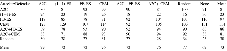
Table 8 presents the average reward from executing 100 episodes of CyberBattleSim. A larger value between agents indicates that one agent outperformed the other. While the absolute rewards offer no interpretation, the relative rewards reflect comparative performance of the algorithms. The standard deviations for these data are given in Table C.1.

Table 8.

The average rewards (rounded to the nearest integer) from 100 episodes in each attacker and defender pairing. The column gives the defender and the row gives the attacker. We include an untrained attacker and defender which randomly select each action as a control as well as an environment with no defender. The averages of each row and column are given at the end. The largest value in each column is bolded to show which attacker performed best against a given defender. The smallest value in each row is underlined to show which defender performed the best against a given attacker

The best-performing attacker is A2C, with an average reward of 349 across all defenders, followed by A2C+FB-ES with 345 and A2C+CEM with 340. The pure ES methods FB-ES and CEM also perform well with 323 and 293, respectively, and (1+1)-ES was only able to achieve an average reward of 98, while the untrained random attacker had an average reward of 38.

Among defenders, A2C+FB-ES performs best, allowing an average reward of 189 (or, alternatively, achieving an average reward of $-189$ ), followed by FB-ES, CEM and A2C+CEM which allow an average reward of 205, 216 and 233, respectively. Notably, A2C+FB-ES also was the best-performing defender against each individual attacker as well. A2C and (1+1)-ES allowed an reward of 296 and 300, performing worse than the untrained random defender which has an average of 279 but better than no defender which has an average of 325. Overall, it appears that A2C+FB-ES is the best-performing defender and is among the best attackers (along with A2C and A2C+CEM).

Reward over time The reward over time versus no defender for the attackers trained using all the algorithms and the regular Type First neural network is shown in Figure 7 (Left). All algorithms except for (1+1)-ES appear to train the attacker to similar final rewards, with A2C, A2C+FB-ES and A2C+CEM having the best stability. The reward over time for each attacker versus the coevolving defender is somewhat uninformative as it depends on the performance of both the attacker and defender. However, by calculating the difference between the attacker’s reward with no defender and the attacker’s reward with the defender, we can obtain a rough heuristic for the defender’s performance over time. This graph is shown in Figure 7 (Right). While significantly more noisy than the previous graph, it appears that A2C+FB-ES performs the best and with the most stability over time, with FB-ES, CEM and A2C+CEM also creating a significant difference in reward. A2C and (1+1)-ES are close to zero for much of the training period.

Figure 7.

(Left) The attacker’s reward over time versus no defender for each algorithm used in training. (Right) The difference in reward between the attacker versus the trained defender and the attacker versus no defender during coevolution. The rewards are smoothed by averaging consecutive terms.

6.3.1 Coevolutionary round-robin training

The reward over time versus no defender for the attackers trained using CEM with and without the round-robin is shown in Figure 8 (Left). The CEM with round-robin appears to overtake the CEM without round-robin during the course of training and finish at a higher average reward. When testing each attacker against both defenders trained with CEM for 100 episodes each, the CEM with round-robin earned an average reward of 234 while the CEM without round-robin earned an average reward of 194.

Figure 8.

(Left) Attacker’s reward at various checkpoints during the 24 hours of training by CEM with and without the round-robin method. (Right) The Attacker’s reward at various checkpoints during the 24 hours of training of A2C+CEM with the ‘Type First’, ‘Target First’, and ‘Simple’ neural network approaches described in Section 4.1. The rewards are smoothed by averaging consecutive terms.

7.1 Experimental comparisons

Our results suggest that the AlphaZero algorithm, which incorporates planning, could be effective in training agent-based Attackers and Defenders both with deep reinforcement learning methods and with gradient-free methods. The different strategies used by the different trained models suggest the emergence varying strategies, even in a simple SNAPT environment. More work is needed to determine whether the different training algorithms tend to converge to consistent but different strategies. Additionally, these results suggest that a training approach using multiple agents, such as a population-based method, might result in robust Attackers and Defenders that are successful against a variety of different strategies. In addition, a game-theoretic analysis to determine optimal strategies may also be possible.

In CyberBattleSim, the Attacker trained with CEM not training in round-robin style was strong. When round-robin competitions were compared, they outperformed the Attacker trained with CEM not training in round-robin style. Note the pairing system used in (1+1)-ES and fitness-based ES (FB-ES) is essentially this round-robin system with only two attackers and defenders. This first suggests the ES with sample size greater than one is advantageous and round-robin play offers even greater advantage.

In the investigation of A2C NN architectures, there was no significant performance difference between the Type First and Target First NNs trained with A2C+CEM. This suggests that this NN architecture design is invariant to a change in element selection. Both the Type First and Target First NNs outperformed the Simple NN architecture, suggesting the multi-stage architecture provides advantage to Attacker policy training in CyberBattleSim. Applying this multi-stage neural network design to agents in other cybersecurity ModSim platforms could provide additional evidence for this hypothesis. We also note that the multi-stage neural network architecture utilizes about 300 000 weights, about 3 times fewer than the 900 000 weights used by the Simple neural network architecture. The extent of this complexity difference would be even greater in larger, more complex simulated environments.

We see that among the algorithms, the best-performing attackers appear to be those trained with deep reinforcement learning (DRL) either solely or in combination with ES. One somewhat surprising result is the apparent instability of the ES algorithms relative to DRL, contradicting the idea that ES may be a more stable alternative to DRL (Mnih et al., Reference Mnih, Kavukcuoglu, Silver, Rusu, Veness, Bellemare, Graves, Riedmiller, Fidjeland, Ostrovski, Petersen, Beattie, Sadik, Antonoglou, King, Kumaran, Wierstra, Legg and Hassabis2015). Among Defenders, the algorithms training with ES solely or in combination with A2C performed best (except for (1+1)-ES). The algorithm only utilizing A2C performed quite poorly relative to the others, possibly due to the relative instability of the environment from the Defender’s perspective. (1+1)-ES performed poorly in both Attacker and Defender settings, likely due to its aggressive update strategy (Lee et al., Reference Lee, Lee, Shin, Kweon, Larochelle, Ranzato, Hadsell, Balcan and Lin2020). Overall, the combined method A2C+FB-ES was among the best algorithms for training both Attackers and Defenders. However we are hesitant to make conclusions about the statistical significance of such results without more information on the stability of each algorithm across training runs.

Table 9.

The average rewards (rounded to the nearest integer) from 100 episodes for each pairing of trained attackers and defenders from the three attacker neural network architectures trained with A2C+CEM. The row gives the attacker and the column gives the defender. The average reward for each attacker is given in the Mean column. The largest value in each column is bolded to show which attacker performed best against a given defender

Table 10.

CyberBattleSim settings. The feature vector observations given to the attacker and defender. The Agent column gives whether the observation is given to the attacker or defender, the Type column gives whether the observation is global or device-specific, the Observation column gives the name of the observation (see Section C), and the Dimension column gives the dimension of the observation. For device-specific observations, the dimension is multiplied by 6 as there are 6 nodes in the network. The total size of the attacker and defender observations is given in the Total row in the observation column

Our results suggest that combining DRL and ES may provide more stable and robust algorithms for training agents in a competitive environment. We find that these algorithms are able to coevolve autonomous attackers to take actions in CyberBattleSim, and that introducing certain specializations such as round-robin evaluation and a multi-stage network architecture may improve performance.

7.2 Limitations and threats to validity

Based on the experimental setup which had each algorithm train only a single neural network, it is premature to draw conclusions about the statistical significance of the results without more information on the stability of each algorithm. While it appears the trained SNAPT models converged to different strategies, it is unclear to what extent this is due to the different training methodologies as opposed to random noise. Training multiple models with each algorithm could provide more insight into the stability of the models.

Simple Network APT (SNAPT) has many simplified assumptions. First, the use of a device (node) value is a simplifying assumption. For example the attribution of events is notoriously hard, both post-incident and during, and without knowledge of the attacker intent it is difficult for a defender to know the value of a device. In addition, it is difficult to ascribe devices intrinsic value to attackers, although information stored on a device, or the abilities provided by the device can provide quantifiable value.

The fixed number of moves make the environment susceptible to the horizon effect that is, an agent who can delay an opponent from reaching a device till past the max number of moves can avoid consequences on their reward. Moreover, the exploit probability is a simple approximation of the notion of a security upper bound, with a securing action not able to exceed the bound. Furthermore, the limited resources of defenders is a very general concept and cannot capture actions that would be obvious in actual networks. For example, if one device controls access to the network or contains the classified document server, the defender would allocate all their securing actions to that device.

CyberBattleSim The formulation of the reward as a zero-sum game is a simplified assumption to the complexity of cybersecurity realities. From a practical view the available actions for a defender in CyberBattleSim somewhat limits the practical use of discovered defender policies, as in practice compromised services are often patched, not only shut down or rebooted. Additionally, currently the agents only work in the particular network they are trained on, and their strategies would be ineffective in a different topology. From a more theoretical standpoint the CyberBattleSim environment has not been analyzed too rigorously, and it has over 1,000 available actions to the attacker which makes analysis quite complex.

7.3 Future work

In future work we will expand and improve the training methods used for better performance in larger, more complex simulations. The input dimension for both attacker and defender neural networks grows linearly with the number of devices in the simulated network, and introducing a recurrent neural network design similar to that used in natural language processing (Palangi et al., Reference Palangi, Deng, Shen, Gao, He, Chen, Song and Ward2016) may provide an effective design whose input dimension size remains small even in large networks. Such a design may also allow for the model to learn general strategies independent of network topology. We will also expand the scope of the algorithms used, including methodologies such as AI planning or population-based evolutionary algorithms which have found success in other domains, in addition to other coevolution setups (Popovici et al., Reference Popovici, Bucci, Wiegand and Jong2012). Moreover, the ability to train agents on multiple scenarios and to transfer policies to unseen scenarios will be investigated. The practical application of the policy search method could be improved by analyzing the discovered policies. Finally, the hyperparameters of the algorithms and the setup can be explored further, for example the training time until convergence.