





1 Introduction
With rapid advances of LLMs in AI, but without assurance in their speedy question answering, rigorous logic inference has become even more important for critical applications. However, understanding drastically different inference methods and their efficiency on different kinds of input data has remained a significant challenge.
Logic rules allow analysis of complex relationships to be expressed easily and precisely, especially with recursive rules for transitive relations in critical applications, for example, understanding program structures, flows, and dependencies (Smaragdakis and Balatsouras Reference Smaragdakis and Balatsouras2015; Flores-Montoya and Schulte Reference Flores-Montoya and Schulte2020); enforcing security policies (Li and Mitchell Reference Li and Mitchell2003; Hristova et al. Reference Hristova, Tekle and Liu2007); probing networking systems including social networks (Loo et al. Reference Loo, Condie, Garofalakis, Gay, Hellerstein, Maniatis, Ramakrishnan, Roscoe and Stoica2009; Seo et al. Reference Seo, Guo and Lam2013); and analyzing knowledge graphs in general (Bellomarini et al. Reference Bellomarini, Sallinger and Gottlob2018; Hogan et al. Reference Hogan, Blomqvist, Cochez, d’Amato, Melo, Gutierrez, Kirrane, Gayo, Navigli and Neumaier2021).
Powerful rule systems allow analysis expressed using rules to be executed automatically without low-level programming. There are not only Prolog systems since the 1970s (Sterling and Shapiro Reference Sterling and Shapiro1994) and answer-set programming (ASP) systems since the 1990s (Gebser et al. Reference Gebser, Kaminski, Kaufmann and Schaub2012), but also more restricted Datalog systems since the 1980s (Maier et al. Reference Maier, Tekle, Kifer and Warren2018) that have been regularly (re)created since the 2000s (Ketsman et al. Reference Ketsman and Koutris2022) due to increasing need of analysis, especially for transitive relations.
How to best utilize the power and efficiency of automatic inference in rule systems? It is regularly observed that different inference methods and rule systems can have significantly different performance, besides requiring different ways to express the analysis:
-
• The same analysis written differently using rules, as well as the same size of input data having different shapes, so to speak, can have drastically different running times. Different inference methods can tolerate these differences very differently.
-
• For applications written using rule languages together with other languages, where input data and analysis results are large, efficiency of passing data and results can also make a large difference, and may dominate the running time.
It is desirable to better understand and predict the efficiency of different inference methods, for different variants of rules running on different kinds of input data of different sizes.
This paper presents a systematic, precise, and detailed comparative analysis of the efficiency of computing transitive relations. We consider all three types of well-known inference methods – query-driven, ground-and-solve, and fact-driven – along with their respective optimizations, across different recursive rules and different input graph types, and compare with optimal complexities for the first time.
We also confirm analyzed results with experiments using rule systems widely considered to have best performances: Prolog system XSB (Sagonas et al. Reference Sagonas, Swift and Warren1994; Swift et al. Reference Swift, Warren, Sagonas, Freire, Rao, Cui, Johnson, de Castro, Marques, Saha, Dawson and Kifer2022) for query-driven, ASP system clingo (Gebser et al. Reference Gebser, Kaminski, Kaufmann and Schaub2019; clingo 2026) for ground-and-solve, and Datalog system Soufflé (Jordan et al. Reference Jordan, Scholz and Subotić2016; Souffle 2026) for fact-driven.
We use the most well-known rules for computing the transitive closure of arbitrary graphs, but our method of calculating optimal complexities and our analyses for all three inference methods and rule variants are general.
-
• The rules for transitive closure are also known for solving graph reachability, the most fundamental problem in analyzing deep relationships, especially with unbounded depth, which makes transitive closure well known to be beyond first-order logic (Grädel Reference Grädel1991).
-
• The rules capture both key features of analyses of transitive relations – join and recursion. Rules with more joins and recursions, over more relations with more arguments, reduce to join and recursion as in the rules for transitive closure (Liu and Stoller Reference Liu and Stoller2009; Liu Reference Liu2013).
-
• The rules have all three variants of recursion – left, right, and double – and their significant impact on efficiency has not been analyzed in prior comparisons except for showing two curves on one ad hoc graph type (Liu et al. Reference Liu, Stoller, Tong, Lin and Tekle2022, Reference Liu, Stoller, Tong and Tekle2023b).
We also examine a wide variety of input graph types, including all from an extensive previous study (Brass and Wenzel Reference Brass and Wenzel2019b).
We present precisely calculated optimal time complexities for all combinations of rule variants and graph types; comparative analysis across different inference methods for all combinations; and confirmation with detailed experiments. In particular, we show how the analyzed complexities explain the sameness and differences in actual query times precisely. These results help predict the efficiency of different inference methods and best utilize different rule systems. We also discovered a performance bug in XSB.
There has been significant bodies of work on both precise complexities and performance measurements, as discussed in Section 6. Our contributions include four main aspects that are studied systematically for the first time.
-
• A comparative analysis across all three types of well-known inference methods, especially with their respective optimizations, and their impact on the complexity and efficiency of analysis of transitive relations.
-
• Precise optimal time complexity calculation for inference for different rule variants and input graph types, not ignoring rule variants and considering only data sizes.
-
• Detailed running time measurements for all of compiling and loading programs, reading input data, querying or grounding and solving, and writing query results.
-
• Confirmation of measured times against analyzed efficiency across all inference methods, rule variants, and graph types, helping best utilize different rule systems and possible improvements.
The rest of the paper is organized as follows. Section 2 compares different inference methods for logic rules and different rule systems and languages supporting the different inference methods. Section 3 explains the rule variants and graph types analyzed and evaluated. Section 4 presents precise optimal time complexity analysis as well as analysis for different inference and optimization methods. Section 5 describes experimental results with key findings and analysis. Section 6 discusses related work, and as conclusion, directions for future work.
2 Comparing Inference Methods and Rule Systems
We consider all three types of drastically different inference methods, used by mostly separate communities of logic rule systems:
-
1. Query-driven inference, also known as goal-directed search or top-down evaluation, the core of Prolog systems and variants (Sterling and Shapiro Reference Sterling and Shapiro1994);
-
2. Ground-and-solve inference, the core of ASP systems (Gebser et al. Reference Gebser, Kaminski, Kaufmann and Schaub2012);
-
3. Fact-driven inference, also called bottom-up evaluation, the core of Datalog systems and variants (Maier et al. Reference Maier, Tekle, Kifer and Warren2018).
We distill and contrast the fundamentals of these different methods, along with their powerful optimizations to overcome their root sources of inefficiency. Their impacts on the efficiency of analysis of transitive relations are described in Sections 4 and 5.
2.1 Inference Methods with Powerful Optimizations
Despite significant differences, all inference methods are aimed at providing the best efficiency. It is the optimized inference that is to be compared with optimal complexities.
2.1.1 Query-Driven Inference
Query-driven inference performs top-down evaluation starting from the given query, searching through rules recursively – querying, in left-to-right order, hypotheses of rules whose conclusion matches the current query – until supporting facts for all queries are found. This goal-directed search allows rules to be used for not only logic programming, but also relational programming as with database languages and recursive programming as with functional languages (Sterling and Shapiro Reference Sterling and Shapiro1994).
However, simple top-down evaluation may not terminate for recursive rules over cyclic relationships, and may take exponential time on acyclic relationships. This is because the same queries may be repeated infinitely or exponentially many times. Top-down evaluation with tabling solves this fundamental problem by remembering the queries performed and reusing the query results (Tamaki and Sato Reference Tamaki and Sato1986; Chen and Warren Reference Chen and Warren1996; Swift and Warren Reference Swift and Warren2012).
2.1.2 Ground-and-Solve Inference
Ground-and-solve inference finds answers to queries by using grounding followed by solving (Kaufmann et al. Reference Kaufmann, Leone, Perri and Schaub2016). Grounding instantiates rules, replacing variables in rules with values that contain no variables, yielding a propositional program. Solving then finds satisfying answers to the propositional program under stable model semantics, by using try-and-backtrack combinatorial search.
However, naive grounding and solving can lead to combinatorial explosion and even nontermination. Optimized grounding tries to consider only possible combinations of values that can match given or derived facts, not all combinations (Kaufmann et al. Reference Kaufmann, Leone, Perri and Schaub2016). Advanced search uses conflict-driven clause learning (CDCL) with back-jumping instead of backtracking, skipping more areas of unfruitful search (Marques-Silva and Sakallah Reference Marques-Silva and Sakallah1999; Gebser et al. Reference Gebser, Kaminski, Kaufmann and Schaub2012).
2.1.3 Fact-Driven Inference
Fact-driven inference performs bottom-up evaluation starting from facts, repeatedly applying rules – inferring new facts from conclusions of rules whose hypotheses match existing facts – until no more new facts can be inferred. This is a least fixed-point computation, with a larger set of facts inferred in each iteration using facts from the previous iteration, until a fixed point is reached.
Naive bottom-up inference from all facts in each iteration can result in heavily repeated computation. Well-known semi-naive evaluation considers only new facts added in each iteration, yielding drastic efficiency improvement (Bancilhon Reference Bancilhon1986). However, it may still have redundant computations in each iteration. Optimal computation using incrementalization with minimum increment considers only one fact in each iteration and avoids all redundant computations, and furthermore gives precise complexity guarantees (Liu and Stoller Reference Liu and Stoller2009; Liu Reference Liu2013).
2.2 Rule Systems and Languages
For confirming analyzed inference efficiency through experiments, we use state-of-the-art rule systems widely considered to have the best performance using different inference methods: Prolog system XSB (Sagonas et al. Reference Sagonas, Swift and Warren1994; Swift et al. Reference Swift, Warren, Sagonas, Freire, Rao, Cui, Johnson, de Castro, Marques, Saha, Dawson and Kifer2022) for query-driven, ASP system clingo (Gebser et al. Reference Gebser, Kaminski, Kaufmann and Schaub2019; clingo 2026) for ground-and-solve, and Datalog system Soufflé (Jordan et al. Reference Jordan, Scholz and Subotić2016; Souffle 2026) for fact-driven.
2.2.1 Unique Advantages
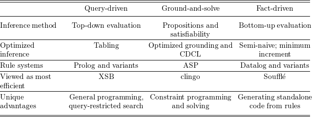
Beyond their shared power, rule systems implementing different inference methods have different unique advantages that are critical for different kinds of applications.
-
• Prolog systems support general-purpose programming. Also, their goal-directed search can answer queries (e.g., only paths from a particular vertex) much more efficiently by inferring only needed facts, not all facts.
-
• ASP systems allow powerful constraint programming and solving for constraint satisfaction and optimization problems (e.g., the traveling salesman problem).
-
• Datalog systems often generate standalone code specialized for the given rules (e.g., code for computing transitive closure) without requiring a general inference system at runtime, for example, Soufflé does so, but XSB and clingo do not.
Table 1 summarizes the inference methods and rule systems. Note that other systems, for example, Ciao and GNU Prolog, can also generate standalone code and support CLP for writing constraints, but they are less efficient; GNU Prolog even requires manual programming for tabling to avoid nontermination or exponential time for recursive rules on graphs.
Inference methods and rule systems

2.2.2 Rule Languages
Largely due to different inference methods used, rule languages supporting these methods have different features. We show this using the transitive closure problem.
Given a predicate, edge, that asserts whether there is an edge from a first vertex to a second vertex, the transitive closure problem defines a predicate, path, that asserts whether there is a path from a first vertex to a second vertex by following the edges. This can be expressed in all dominant logic languages, including Prolog, ASP, and Datalog variants, as follows:

Often, the name reachable is used in place of path.
Besides the two rules above, different rules languages require different additional specifications.
-
• Prolog systems like XSB. To avoid nontermination or exponential time, tabling directives are needed, as follows for using default tabling for predicate path:

Also, to return all facts of path with query-driven inference, additional rules like the following can be used, employing fail to continue the search for each next path fact until no more can be found and then the last printPath succeeds.
-
• ASP system clingo. With ground-and-solve, by default all facts will be returned. To get back only facts of path, the following additional directive can be used:
-
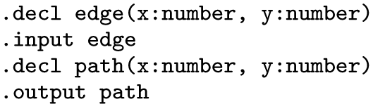
• Datalog system Soufflé. To compile Datalog rules to standalone code in C++, which is then compiled and run, additional type and input–output declarations are needed:



Additionally, Prolog systems like XSB are highly powerful and expressive, and can be used for direct scripting and timing for performance analysis. In contrast, ASP and Datalog languages like clingo and Soufflé have more limited features and rely on a host language – Python for clingo and C++ for Soufflé – for application development.
3 Rule Variants and Input Graph Types
We consider subtly different rule variants and a wide variety of graph types that may affect efficiency of inference methods, drastically.
3.1 Variants of Rules
It is long known that different variants of rules for solving the same problem can have drastically different performance, but this has not been studied precisely in general. We consider all three well-known variants of rules for transitive closure:
-
1. Left recursion: the recursive rule can be written differently, by switching the two predicates, so that the recursive occurrence of path is on the left:
-
2. Right recursion: the recursive rule as written in Section 2 has recursive occurrence of path on the right.
-
3. Double recursion: the recursive rule can also be written by replacing edge with path, yielding two recursive occurrences of path:


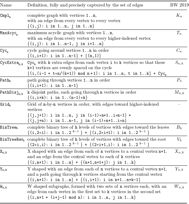
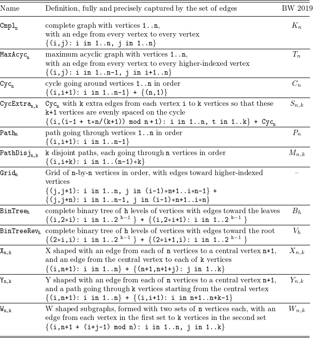
Kinds of input graphs and their definitions, with their names if any in Brass and Wenzel (Reference Brass and Wenzel2019b)
3.2 Kinds of Input Graphs
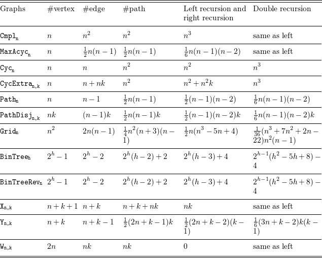
We consider and precisely define 12 different kinds of graphs, shown in Table 2. It includes all 11 kinds in rbench (Brass and Wenzel Reference Brass and Wenzel2019b), created to address the issues with input in OpenRuleBench (Liang et al. Reference Liang, Fodor, Wan and Kifer2009). We created the last one, grid, with more rigid and intertwined edges. Together, they aim to capture graphs of different shapes that may affect the efficiency of computing the transitive closure very differently.
Note that n is just one of the parameters, and is not always the number of vertices in the graph, although it is for the first 5 graph types in Table 3. Table 3 columns 2 and 3 show the precise numbers of vertices and edges.
Optimal number of combinations for all 3 recursion variants and all 12 graph types

Table. 3. Long description
The table compares the number of vertices, edges, paths, and optimal combinations for different graph types and recursion variants. It has 12 rows and 5 columns. The columns are labeled Graphs, #vertex, #edge, #path, and Left recursion and Double recursion right recursion. The rows are labeled with different graph types: CmpIn, MaxAcyc, Cyc, CycExtra, Path, PathDisj, Grid, BinTree, BinTreeRev, Xn,k, Yn,k, Wn,k. Each row provides specific values for the number of vertices, edges, paths, and optimal combinations for each graph type and recursion variant. The table includes various mathematical expressions and formulas to represent these values.
4 Analysis of Optimal Time Complexities
To compute all facts that can be inferred, any inference using bottom-up, group-and-solve, or top-down methods must consider all combinations of given and inferred facts that can make all hypotheses of a rule become true. Each such combination leads to a rule firing.
Optimality in considering such combinations can be achieved by using the method of incrementalization with minimum increment (Liu and Stoller Reference Liu and Stoller2009; Liu Reference Liu2013). The method allows each combination to be considered at most once and in worst-case $O(1)$
time – by considering only one fact at a time and using indexing to find each new combination with the fact in
$O(1)$
time – by considering only one fact at a time and using indexing to find each new combination with the fact in $O(1)$
time.
$O(1)$
time.
4.1 Optimal Number of Combinations
For computing all path facts, for all three rule variants, the first rule is fired once for each edge fact, totaling to be #edge, the number of edges. For the second, recursive rule, we calculate the exact number of combinations for each graph type and each rule variant. The calculation, for each graph type and each rule variant, first forms a precise formula for the exact counting and summing, and then simplifies the formula to a closed form using Mathematica. Details of the calculation are in an appendix of Liu et al. (2026).
Table 3 shows the resulting precise complexity formulas in closed forms for the recursive rule. The particular closed forms in Table 3 were selected and rearranged manually to have a consistent factor representation across all rule variants and graph types.
Despite all the differences among the kinds of graphs listed, there are a number of interesting equalities to observe. For example, for Cmpl graphs, the number of combinations is the same for all different recursions, and this is also the case for MaxAcyc, X, and W graphs.
It is particularly interesting to see that for all graph types, left and right recursions lead to the same number of combinations. This is easy to see for graphs with a kind of symmetry between paths going into an edge (left recursion) and paths coming out (right recursion), which include the first 7 graph types. It is also easy to see for $\texttt {X}_{\texttt {}}$
and
$\texttt {X}_{\texttt {}}$
and $\texttt {W}_{\texttt {}}$
graphs, which are the simplest cases with only paths of lengths 2 and 1, respectively.
$\texttt {W}_{\texttt {}}$
graphs, which are the simplest cases with only paths of lengths 2 and 1, respectively.
However, $\texttt {BinTree}_{\texttt {h}}$
and
$\texttt {BinTree}_{\texttt {h}}$
and $\texttt {BinTreeRev}_{\texttt {h}}$
do not have such symmetry, similar to
$\texttt {BinTreeRev}_{\texttt {h}}$
do not have such symmetry, similar to $\texttt {Y}_{\texttt {n,k}}$
not having such symmetry. It still happens to be that even for left or right recursion alone,
$\texttt {Y}_{\texttt {n,k}}$
not having such symmetry. It still happens to be that even for left or right recursion alone, $\texttt {BinTree}_{\texttt {h}}$
and
$\texttt {BinTree}_{\texttt {h}}$
and $\texttt {BinTreeRev}_{\texttt {h}}$
have the same number of combinations despite they are from very different summation formulas. Consider the right recursion form edge(X,Y), path(Y,Z).
$\texttt {BinTreeRev}_{\texttt {h}}$
have the same number of combinations despite they are from very different summation formulas. Consider the right recursion form edge(X,Y), path(Y,Z).
-
• For
$\texttt {BinTree}_{\texttt {h}}$
, consider i-1 levels of edges from root to leaves, with i from 1 to h-1. At the ith level of edges, there are 2
$^{\tt i}$
edges. For each such edge (u,v), there is a path from v to each vertex in the subtree rooted at v except for v. The subtree has 2
$^{\tt h-i}$
-1 vertices, and the connecting vertex itself should also be subtracted. Thus, the number of combinations for edge(X,Y), path(Y,Z) is
$ \sum _{i = 1..h-1} 2^i * (2^{h-i}-2)$
. -
• For
$\texttt {BinTreeRev}_{\texttt {h}}$
, consider i-1 levels of edges from leaves to root, with i from h to 2. At the ith level of edges, there are 2
$^{\tt i-1}$
edges. For each such edge (u,v), there is a path from v to each vertex above it in the path to root. There are i-2 such vertices. Thus, the number of combinations for edge(X,Y), path(Y,Z) is
$ \sum _{i = h..2} 2^{i-1} * (i-2)$
.






Both actually simplify to the same closed form as in Table 3. Because of this same closed form, left and right recursions for both kinds of trees have the same closed form too. When we found that left and right recursions for Y graphs also have the same closed form, it became curious, and we prove the following general result for directed trees; the result actually applies to $\texttt {Path}_{\texttt {n}}$
,
$\texttt {Path}_{\texttt {n}}$
, $\texttt {PathDisj}_{\texttt {n,k}}$
, and the last 5 graph types.
$\texttt {PathDisj}_{\texttt {n,k}}$
, and the last 5 graph types.
We prove that for any directed tree, left and right recursions have the same number of combinations. Precisely, let vert be the set of vertices in the given edge relation, then
 \begin{align*} &\sum _{\texttt {v} \in \texttt {vert}} \#\{\mathtt {u\!:\,path(u,v)}\} \times \#\{\mathtt {w\!:\,edge(v,w)}\}\\ &\quad= \sum _{\texttt {v} \in \texttt {vert}} \#\{\mathtt {u\!:\,edge(u,v)}\} \times \#\{\mathtt {w\!:\,path(v,w)}\} \end{align*}
For any directed tree, there is at most one path between any two vertices. Consider any matching path(u,v) and edge(v,w) from left recursion. Let edge(u,v1) be the unique edge on the path from u to v. Then there is the unique path(v1,v) joining with edge(v,w) giving the unique path(v1,w). Now the matching edge(u,v1) and path(v1,w) must be counted in right recursion. Thus each combination path(u,v) and edge(v,w) from left recursion corresponds to a unique combination edge(u,v1) and path(v,w) from right recursion. Symmetrically, each combination from right recursion corresponds to a unique combination from left recursion. Thus, the equation holds.
Note that the equation does not hold for all graphs. An example is a graph with edges {(1,2), (2,1), (1,3), (2,3)}. The combinations path(1,1), edge(1,2) and path(1,1), edge(1,3) are not captured in right recursion, because there is no edge (1,1) or (2,2).
4.2 Time Complexities of Different Inference Methods
Despite that optimal complexities are achieved with incrementalization-based method (Liu and Stoller Reference Liu and Stoller2003, Reference Liu and Stoller2009) and confirmed experimentally (Liu and Stoller Reference Liu and Stoller2009), implementations using other inference methods have different other cost issues.
-
1. Query-driven inference with tabling has separate overhead from general mechanisms for table maintenance and lookup. However, this is minimal, but the following is a significantly larger cost issue.
The inference considers hypotheses of a rule from left to right, so the order of the two predicates matters. Contrary to common belief, left recursion is the most efficient for table lookup, as analyzed precisely in Tekle and Liu (Reference Tekle and Liu2010); the key idea is that, with left recursion, the search for path(X,Y) looks up path(X,Z) in the same table due to the same value of X. With right recursion, it needs to look up path(Z,Y) in a different table for each different value of Z from edge(X,Z) on the left; this is also the case with double recursion except that the Z is from path(X,Z), which could be asymptotically larger than from edge(X,Z) depending on the input graph.
-
2. Ground-and-solve with optimized grounding and solving generally has a separate cost tracking ground rules rather than directly returning the derived facts. This is not minimal but relatively small. For recursive rules with no negation, grounding does iterative evaluation on ground rules and computes all resulting facts.
A larger cost issue is similar to the issue with recursion variants for query-driven inference above, because grounding also considers hypotheses in a rule from left to right (Kaufmann et al. Reference Kaufmann, Leone, Perri and Schaub2016). Additionally, despite extensive optimizations, iterative evaluation on ground rules uses semi-naive evaluation (Kaufmann et al. Reference Kaufmann, Leone, Perri and Schaub2016), another larger cost issue as described for fact-driven inference below.
-
3. Fact-driven inference with semi-naive evaluation has redundant computations and overhead from considering all new facts in each iteration. This is because it goes through an extra set, and there could be repeated computations within the processing of a set instead of one element (Cai and Paige Reference Cai and Paige1988), unlike incrementalization with minimum increment (Liu and Stoller Reference Liu and Stoller2009; Liu Reference Liu2013). It could be asymptotically worse than optimal without prudent incremental processing of the extra set.
However, in contrast to the two methods above, inference driven by newly inferred facts of a predicate, for example, path, can have the same efficiency regardless of whether the predicate is in a left or right recursion to join with another predicate.
Finally, fact-driven inference often generates standalone code from rules, which has a separate cost of compilation, but this is needed only once for each program.
Note that the precise formulas in Table 3 support comparisons of not only asymptotics but also constants. For example, for Cmpl graphs, all three recursion variants have exactly the same number; in comparison, for MaxAcyc with about 1/2 the size of input (edge) and output (path), left and right recursions have about 1/6 of the number of combinations, whereas double recursion has the same number. Section 5 shows through experiments how difference inference methods and systems match the analytical results in this section.
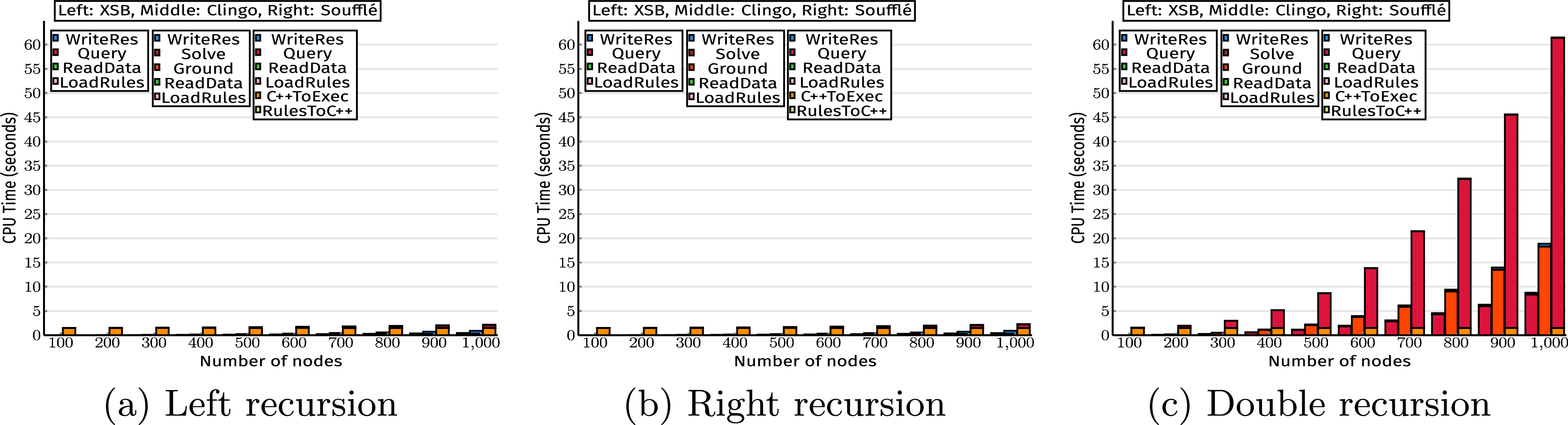
Running times on Cmpl graphs, up to 1000 vertices, 1000000 edges.

Fig. 1. Long description
Three bar graphs depict CPU times for complete graphs of different numbers of nodes across three recursion types: left recursion, right recursion, and double recursion. Each graph has the same structure, with the horizontal axis labeled Number of nodes from 100 to 1000 and the vertical axis labeled CPU Time in seconds. Each graphs compare three systems: XSB, clingo, and Souffle, with each system represented by a different color bar. Bar graph (a) shows left recursion, bar graph (b) shows right recursion, and bar graph (c) shows double recursion. Each graph includes a legend indicating different operations such as LoadRules, ReadData, Ground, Solve, WriteRes. In all bar graphs, the CPU time increases as the number of nodes increases. XSB consistently shows the highest lowest CPU times across all recursion types and node counts, while XSB and clingo and Souffle show lower and more varied CPU times. The trends indicate that double recursion results in the highest CPU times for all systems, followed by right recursion and then left recursion.
Running times on Path graphs, up to 1000 vertices, 999 edges.

Fig. 2. Long description
Three bar graphs depict CPU times for path graphs of different numbers of nodes across three recursion types: left recursion, right recursion, and double recursion. Each graph has the same structure, with the horizontal axis labeled Number of nodes from 100 to 1000 and the vertical axis labeled CPU Time in seconds. Each graphs compare three systems: XSB, clingo, and Souffle, with each system represented by a different color bar. Bar graph (a) shows left recursion, bar graph (b) shows right recursion, and bar graph (c) shows double recursion. Each graph includes a legend indicating different operations such as LoadRules, ReadData, Ground, Solve, WriteRes. In all bar graphs the CPU time increases as the number of nodes increases. In bar graphs (a) and (b), the CPU times for all systems remain relatively low and constant across the number of nodes. In bar graph (c), the CPU times increase significantly with the number of nodes, especially for the Souffle system, indicating a higher computational cost for double recursion.
5 Key Findings from Experimental Results and Analysis
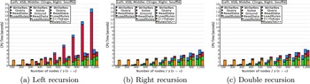
We designed and performed detailed experiments with all three rule systems XSB, clingo, and Soufflé, all three rule variants, and all 12 input graph types. The programs, variants of each, and graphs are exactly as described in Sections 2.2 and 3. For example, Figures 1 and 2 show running times on Cmpl and Path graphs for all recursion types in all three rule systems. Details of the experiments and results are in an appendix in Liu et al., (2026). Key findings from comparing and confirming the analyzed results with the experimental results are as follows:
-
1. Overall, precise calculation of optimal complexity and dedicated analysis of different inference and optimization methods in Section 4 help tremendously in predicting their performances and understanding the differences, for both asymptotic trends and constant factors, across not only the inference and optimization methods but also rule variants and graph types.
-
2. Which inference method and system to use depends on the unique features and powers the method and system provide, including the advantages summarized in Table 1. Whichever method and system are used, the rule variants and input graph types can affect the performance much more, as described below.
-
3. Efficient recursion types depend on the inference method and system. Except for an XSB performance bug discovered for the simplest case (left recursion on
$\texttt {W}_{\texttt {n,k}}$
), described below, and relatively small XSB and Soufflé variations on the next simplest case (left recursion on
$\texttt {X}_{\texttt {n,k}}$
), (1) for XSB and clingo, left recursion is fastest; (2) for Soufflé, left and right recursions are about the same, faster than double recursion; and (3) overall, left recursion is fastest, double recursion can be asymptotically slower, all as analyzed in Section 4. -
4. On all graphs except for left recursion on
$\texttt {W}_{\texttt {n,k}}$
due to the performance bug, XSB, with query-driven inference with tabling, is the fastest, by several times or even an order of magnitude. clingo is the next fastest except for right recursion for Cmpl (e.g., Figure 1) and MaxAcyc where Soufflé is faster. Soufflé is fastest in reading data and writing results (e.g., Figure 3), even if it has the extra compilation time.Fig. 3.Running times on W graphs, up to 2000 vertices, 1000000
$(k = n = 1000)$
edges.We discovered the XSB performance bug when running on
$\texttt {W}_{\texttt {n,k}}$
with increasing k = n (Figure 3). This is the simplest case of all graph types, where path is exactly edge with no extra paths at all, but XSB on left recursion is drastically slower than analyzed. XSB team confirmed this performance bug and analyzed that it is due to hash collisions in this case. -
5. Besides fixing the XSB bug, XSB and clingo could be improved by automatically converting right recursion to left recursion (Tekle et al. Reference Tekle, Hristova and Liu2008). clingo’s right and double recursions could perhaps be improved, possibly with better incremental processing for later hypotheses in a rule. Soufflé has opportunities to become faster in general, for all recursion types, because generated C++ code can be specialized to be much faster than general evaluator code (Rothamel and Liu Reference Rothamel and Liu2007).





We also used well-known graph generators designed to simulate real-world networks and experimented with all three recursion types using all three rule systems. Figure 4 shows the running times on directed Barabási-Albert (BA) graphs (Albert and Barabási Reference Albert and Barabási2002), the most famous model for explaining the scale-free nature of the Internet, World Wide Web, social media, and citation networks. The graphs are generated using the widely-used library NetworkX with preferential attachment parameter value 2.
The results in Figure 4 are consistent with everything we have analyzed, in terms of relative performances of all recursion types and all systems, including a similar performance anomaly in left recursion in XSB as W graphs in Figure 3. We think the anomaly is due to the same reason, because BA graphs are known to have ultra-small path lengths, with average length growing logarithmically with the number of vertices, whereas W graphs have only paths of length 1, so the anomaly for BA graphs is not as serious as for W graphs.
Running times on BA graphs, up to 100000 vertices, 200000 edges.

Fig. 4. Long description
Three bar graphs depict CPU times for BA graphs of different numbers of nodes across three recursion types: left recursion, right recursion, and double recursion. Each graph has the same structure, with the horizontal axis labeled Number of nodes from 100 to 1000 and the vertical axis labeled CPU Time in seconds. Each graphs compare three systems: XSB, clingo, and Souffle, with each system represented by a different color bar. Bar graph (a) shows left recursion, bar graph (b) shows right recursion, and bar graph (c) shows double recursion. Each graph includes a legend indicating different operations such as LoadRules, ReadData, Ground, Solve, WriteRes. In all bar graphs the CPU time increases as the number of nodes increases. XSB is the fastest for right and double recursion and slowest in left recursion. clingo query time is faster than Souffle for all recursion types. Souffle query time grows much higher in double recursion.
6 Related Work and Conclusion
There has been extensive study of efficiency of inference methods and systems, from performance benchmarking to complexity analysis. We discuss closely related works.
Prolog has had benchmarks for comparing performance of different implementations, for example, (CMU AI Repository 1985; CHINA 2001). Some are focused on a special class of problems, for example, interpreters written in Prolog (Körner et al. Reference Körner, Schneider and Leuschel2020). Some are for evaluating the performance of a particular implementation, for example, SWI Prolog (SWI-Prolog bench 2026).
There are also works that evaluate queries in more general rule engines and database systems, for example, the LUBM benchmark (Guo et al. Reference Guo, Pan and Heflin2005) and its extensions (Ma et al. Reference Ma, Yang, Qiu, Xie, Pan and Liu2006; Singh et al. Reference Singh, Bhatia and Mutharaju2020) for OWL on a range of systems, and evaluations including SQL with rules (Brass and Wenzel Reference Brass and Wenzel2019a, Reference Brass and Wenzel2019b). In particular, rbench (Brass and Wenzel, Reference Brass and Wenzel2019b) considers 11 types of graphs, and we use all of them.
OpenRuleBench (Liang et al. Reference Liang, Fodor, Wan and Kifer2009) was extensively constructed for comprehensively evaluating a wide range of systems on a diverse set of problems. Benchmarking (Liu et al. Reference Liu, Stoller, Tong and Tekle2023b) for Alda (Liu et al. Reference Liu, Stoller, Tong and Lin2023a) used all OpenRuleBench benchmarks and more to evaluate an extension of DistAlgo (Liu et al. Reference Liu, Stoller and Lin2017)/Python with Datalog rules that implements queries using XSB, and to compare with programs written purely in Python, DistAlgo, and XSB.
More studies of methods and systems compare on some chosen workloads, for example, Flan (Abeysinghe et al. Reference Abeysinghe, Xhebraj and Rompf2024) on adding and compiling Datalog to Scala compares with Soufflé and two Datalog systems embedded in Rust, Crepe and Ascent, on program analysis; BMLP (Ai and Muggleton Reference Ai and Muggleton2024) on using Boolean matrix operations for rules compares with Soufflé, clingo, B-Prolog, and SWI-Prolog on rules for graphs.
Datalog systems are increasingly studied (Maier et al. Reference Maier, Tekle, Kifer and Warren2018; Vianu Reference Vianu2021; Ketsman et al. Reference Ketsman and Koutris2022), for example, Ketsman et al. (Reference Ketsman and Koutris2022) focuses on 9 Datalog systems including Soufflé, among 17 Datalog engines and more mentioned, and discusses the extensively used semi-naive evaluation and more. There are also dedicated works on evaluating their performances, for example, (Fan et al. Reference Fan, Mallireddy and Koutris2022; Qureshi and Faber Reference Qureshi and Faber2024). In particular, Fan et al. (Reference Fan, Mallireddy and Koutris2022) studies semi-naive execution profile, running time, CPU utilization, and memory consumption on transitive closure and four other closely related problems on binary relations.
None of the existing works analyzes and compares together all three widely different inference methods and their optimizations that make large performance impacts. Also, none of them analyzes different rule variants for the same problem and their significant performance differences. Furthermore, none of them studies precise optimal complexities, or performs detailed measurements from compiling and loading programs to writing query results, let alone confirming measurements against the complexities across inference methods, rule variants, and input graph types.
McAllester (Reference McAllester1999) and Ganzinger and McAllester (Reference Ganzinger and McAllester2002) analyze complexities of bottom-up evaluation using prefix firing counting. Liu and Stoller (Reference Liu and Stoller2003, Reference Liu and Stoller2009) develop systematic incrementalization to automatically transform Datalog rules into efficient implementations with precise time and space guarantees for optimality and trade-offs. Tekle and Liu (Reference Tekle and Liu2010, Reference Tekle and Liu2011) precisely analyze complexities of top-down evaluation for demand-driven queries and develop demand transformations for bottom-up evaluation, improving over magic-set transformations exponentially in program size.
These studies of complexity analysis have been essential for the optimal complexity calculation in this paper, and for precisely understanding the efficiency of top-down query-driven evaluation with tabling versus bottom-up fact-driven evaluation. Their extensions to handle unrestricted negation, quantification, and aggregation, following a powerful unified semantics for them (Liu and Stoller Reference Liu and Stoller2020, Reference Liu and Stoller2022), will be essential for critical applications that need those features.
6.1 Conclusion, limitations, and future works
We have presented a systematic study of efficiency of analysis of transitive relations using different inference methods for different rule variants and input relationship graphs. Despite the compelling results for better understanding and utilizing different rule systems, this work has several limitations, leaving many avenues for future work.
First, in the experiments, the degree of superlinearity and constant costs are not analyzed systematically; analyzing them systematically can help better understand and optimize rule systems.
Second, the study is only about time efficiency; space (Liu and Stoller Reference Liu and Stoller2009; Tekle and Liu Reference Tekle and Liu2010, Reference Tekle and Liu2011), including cache effect on large data, and other measures (Fan et al. Reference Fan, Mallireddy and Koutris2022) are important too. Also important are additional system-specific aspects that affect performance, for example, XSB has subsumptive tabling (which is faster in some cases than default tabling) (Swift and Warren Reference Swift and Warren2012), indexing directives, many input/output functions (for efficiency in different cases), and more (Swift et al. Reference Swift, Warren, Sagonas, Freire, Rao, Cui, Johnson, de Castro, Marques, Saha, Dawson and Kifer2022).
Third, comparative analysis of different methods for demand-driven queries, not inferring all facts, needs to be studied. Demand transformations (Tekle and Liu Reference Tekle and Liu2010, Reference Tekle and Liu2011) would help clingo and Soufflé ; otherwise, goal-directed queries in XSB would perform drastically better. Magic sets in the intelligent grounder of DLV (Calimeri et al. Reference Calimeri, Fuscà, Perri and Zangari2017) and in Soufflé (2026) are important for practical efficiency. Transforming into best recursion variants (Tekle et al. Reference Tekle, Hristova and Liu2008) will also help significantly, as well as employing modular approaches, e.g, Hu et al. (Reference Hu, Motik and Horrocks2022).
Finally, our comparative analysis is only for analyzing transitive relations; many more analysis problems can be added, especially those with negation and aggregation in existing rule systems (Sagonas et al. Reference Sagonas, Swift and Warren1994; Jordan et al. Reference Jordan, Scholz and Subotić2016; Gebser et al. Reference Gebser, Kaminski, Kaufmann and Schaub2019) and even quantification, all unrestricted.
Supplementary material
To view supplementary material for this article, please visit https://doi.org/10.1017/S1471068426100623
 (k=n=1000)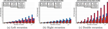


 Open access

