








Impact statement
Reliable prediction of aerodynamic loads is essential for the design, operation, and lifetime assessment of wind turbines. These loads strongly depend on inflow conditions, which are not accessible in operating conditions, as only limited surface signals are typically available. This work introduces a low-cost model combining reduced-order modeling and shallow neural networks to capture the instantaneous nonlinear relationship between measurements and the flow field. The model is trained and tested on numerical results over a wide range of angles of attack representative of the operating conditions. It achieves accurate reconstruction and generalization and also correctly infers the angle of attack from instantaneous data, thus enabling new opportunities for monitoring and control in wind energy systems.
1. Introduction
In the context of wind energy, accurate prediction of mean and instantaneous wind turbine aerodynamic loads is essential for ensuring the structural integrity and efficiency of wind turbines, particularly during gusts or dynamic stall. Originally introduced by Glauert (Reference Glauert1935), the Blade Element Momentum (BEM) method has long been the workhorse for aerodynamic load prediction. Its appeal lies in its simplicity and computational efficiency, assuming a stationary and uniform inflow. Over the decades, BEM has been refined with numerous corrections to account for three-dimensional effects such as tip losses (Prandtl and Betz, Reference Prandtl and Betz1927), root effects (Chaviaropoulos and Hansen, Reference Chaviaropoulos and Hansen2000), yawed inflow (Madsen et al., Reference Madsen, Larsen, Pirrung, Li and Zahle2020), and dynamic inflow conditions (Snel and Schepers, Reference Snel and Schepers1995). Based on comparisons with large-scale field test campaigns (Potentier et al., Reference Potentier, Braud, Guilmineau, Finez and Le Bourdat2021), identified the most impactful corrections and demonstrated that, when supplemented with unsteady aerodynamic models, BEM can reliably capture mean load trends in most conditions. However capturing instantaneous loads remains an important challenge, as it requires knowledge of the surrounding flow field—information that is challenging to access in practical or in situ settings where only sparse, low-resolution wall-pressure measurements are typically available.
The field of sparse flow reconstruction, where a reliable estimator of the flow is built using only limited or noisy measurements, has been widely studied over the last few decades in many engineering applications, ranging from medical diagnostics to atmospheric measurements. In the medical field, the spatially and temporally limited acquisition of the four-dimensional flow magnetic resonance imaging (4D MRI) is complemented by flow reconstruction techniques to determine blood flow during cerebral aneurysms (Zhang et al., Reference Zhang, Brindise, Rothenberger, Markl, Rayz and Vlachos2022). Reconstruction of turbulent flows from restricted observations is also crucial for climatology (Schneider et al., Reference Schneider, Lan, Stuart and Teixeira2017), weather forecast (Kalnay, Reference Kalnay2002), atmospheric (Kaimal and Finnigan, Reference Kaimal and Finnigan1994) and urban boundary layers studies (Blackman and Perret, Reference Blackman and Perret2016; Lu and Papadakis, Reference Lu and Papadakis2023), where metrology techniques (meteorological masts, LIDAR, pressure balloons) give access to only a small fraction of the atmospheric volume of interest. The same problem applies in wind energy when estimating the inflow wind or the downstream wake for both wind turbines and wind farms using high-frequency SCADA data on the turbines (Rott et al., Reference Rott, Petrovi’c and Kühn2020).
As only limited data is accessible in an experiment, there is a need to rely on extensive numerical simulations. For high Reynolds number flows that characterize wind energy studies, the extensive computational cost of Large-Eddy Simulations (LES) makes their applicability difficult in a multi-configuration context. On the other hand, Unsteady Reynolds-Averaged Navier Stokes (URANS) simulations represent a high-fidelity computational tool that was shown to capture satisfactorily the main features of experimental data (Neunaber et al., Reference Neunaber, Danbon, Soulier, Voisin, Guilmineau, Delpech, Courtine, Taymans and Braud2022; Vitulano et al., Reference Vitulano, De Tavernier, De Stefano and von Terzi2025). URANS, therefore, appears particularly relevant to study real-life configurations, as it provides a good trade-off between accuracy and relevance for industrial applications (Sahebzadeh et al., Reference Sahebzadeh, Rezaeiha and Montazeri2022).
Several challenges for flow reconstruction need to be addressed. First, the target flow field to estimate is often turbulent and therefore is characterized by high-dimensional data, which generally needs to be reduced to a more compact representation. Second, physical and economic constraints can limit the number, position, and acquisition rate of the sensors so that optimization strategies may be needed (Hollenbeck et al., Reference Hollenbeck, Grandhi, Hansen and Pankonien2024; Bukowski et al., Reference Bukowski, Rennie and Gordeyev2025). Third, the mapping between the observations and the target field may be nonlinear, as for instance in the reconstruction of a velocity field from pressure measurements (Graziani et al., Reference Graziani, Kerhervé, Martinuzzi and Keirsbulck2018). Finally, an adequate compromise should be found between the cost and the accuracy of the estimation technique.
Comprehensive reviews of sparse reconstruction methodologies can be found in Manohar et al. (Reference Manohar, Brunton, Kutz and Brunton2018), Callaham et al. (Reference Callaham, Maeda and Brunton2019), and Nair and Goza (Reference Nair and Goza2020), but a few key principles are worth recalling here. The majority of approaches rely on Reduced-Order Models (ROMs) to project the high-dimensional flow dynamics onto a low-order manifold. The reconstruction task then reduces to estimating the reduced state, which can subsequently be mapped back to the full-order field. The projection of the high-dimensional dynamics of the complex flow field can be carried out using a linear decomposition basis that can be data-agnostic, such as Fourier modes or wavelets, or data-driven, such as Proper Orthogonal Decomposition, aka POD (Lumley, Reference Lumley, Iaglom and Tatarski1967), or Dynamic Mode Decomposition aka DMD (Schmid, Reference Schmid2010). A comprehensive review of modal decompositions can be found in Taira et al. (Reference Taira, Brunton, Dawson, Rowley, Colonius, McKeon, Schmidt, Gordeyev, Theofilis and Ukeiley2017). However, linear reconstructions may be limited in their ability to capture nonlinear flow features. This has motivated the development of more sophisticated methods, such as sparse regression techniques, to address these issues (Loiseau et al., Reference Loiseau, Noack and Brunton2018).
Generally speaking, recent advances in machine learning have opened new perspectives for flow reconstruction: neural-network-based approaches can learn nonlinear mappings between sparse measurements and the full-order flow, although linear expansions can still be used to reduce the dimensionality of the data (Swischuk et al., Reference Swischuk, Mainini, Peherstorfer and Willcox2019). In particular, efficient models have been constructed by blending deep learning strategies with reduced-order models based on Proper Orthogonal Decomposition, such as the POD-NN method (Hesthaven and Ubbiali, Reference Hesthaven and Ubbiali2018), the POD-DL-ROM method (Fresca and Manzoni, Reference Fresca and Manzoni2022), or the FastSVD-ML-ROM method (Drakoulas et al., Reference Drakoulas, Gortsas, Bourantas, Burganos and Polyzos2023). Among the various neural network architectures that have attracted interest, autoencoders have shown promise for discovering nonlinear manifolds with improved reconstruction accuracy compared to linear subspaces (Lee and Carlberg, Reference Lee and Carlberg2019; Xu and Duraisamy, Reference Xu and Duraisamy2020; Tan, Reference Tan2023) and can provide causality insights (Fukami and Taira, Reference Fukami and Taira2025). Murata et al. (Reference Murata, Fukami and Fukagata2020) showed that a convolutional neural network autoencoder was able to provide a more compact representation than POD. Graph neural networks (GNNs) have also been shown to be a versatile and powerful tool for estimation purposes, as was recently evidenced by Duthé et al. (Reference Duthé, Abdallah, Barber and Chatzi2023), who developed a message-passing GNN to predict steady two-dimensional pressure and velocity fields from surface pressure distributions around airfoils of arbitrary shape.
Possible drawbacks of data-driven neural frameworks include their lack of interpretability and their disconnection from physics-based knowledge. These limitations are addressed by Physics-Informed Neural Networks (PINNs), introduced by Raissi et al. (Reference Raissi, Perdikaris and Karniadakis2019), which are trained with a loss that seeks to both minimize the discrepancy with the observations and to enforce physics conservation laws. Implementations included velocity reconstruction in a cylinder wake from sparse and incomplete velocity measurements (Xu et al., Reference Xu, Sun, Huang, Guo, Yang and Ju2023), bluff-body wake and Kolmogorov flow reconstruction with a Convolution Neural Network trained for various physics-based loss formulations (Mo and Magri, Reference Mo and Magri2025), and reconstruction of three-dimensional turbulent wall-bounded flows from two-dimensional planar measurements with a physics-constrained variational autoencoder (Hora et al., Reference Hora, Gentine, Momen and Giometto2024). However, while PINNs show great potential, they can induce high computational costs, and can struggle on complex flows, such as multi-scale dynamic systems (Li et al., Reference Li, Zheng, Kovachki, Jin, Chen, Liu, Azizzadenesheli and Anandkumar2024).
In contrast, a low-cost alternative that has shown substantial promise is the shallow neural network model introduced by Erichson et al. (Reference Erichson, Mathelin, Yao, Brunton, Mahoney and Kutz2020) (referred therein as “shallow decoder,” an denoted as SNN by Carter et al. (Reference Carter, De Voogt, Soares and Ganapathisubramani2021)), which relies on a simple neural architecture to map sparse sensor inputs to high-dimensional flow fields. The shallow neural network model has demonstrated superior performance compared to POD-based linear reconstructions in test cases such as flow past a cylinder, sea-surface temperature dynamics, and synthetic turbulence (Erichson et al., Reference Erichson, Mathelin, Yao, Brunton, Mahoney and Kutz2020). Shallow neural networks have further been used as nonlinear refinements of linear state estimation (Carter et al., Reference Carter, De Voogt, Soares and Ganapathisubramani2021) or as ROM-based models for reconstructing vorticity fields from vorticity- and surface stress-measuring sensors on the body of the flat plate at high angle of attack (Nair and Goza, Reference Nair and Goza2020). The framework of shallow neural networks has also been extended to take into account temporal information. Williams et al. (Reference Williams, Zahn and Kutz2024) successfully tested a shallow recurrent decoder (SHRED) that relies on sensor past history for reconstruction and forecasting tasks. This approach can be complemented by a ROM (SHRED-ROM, Kutz et al., Reference Kutz, Reza, Faraji and Knoll2024; Tomasetto et al., Reference Tomasetto, Williams, Braghin, Manzoni and Kutz2025). However, application of these tools requires extensive knowledge about the environmental parameters, which may vary significantly and/or be inaccessible in the industrial context of wind energy. In particular, the bandwidth and memory requirements of commercial sensors may be insufficient to provide accurate information about their time evolution. As a consequence, we will assume that the temporal continuity of the information cannot be guaranteed and only consider instantaneous reconstruction strategies in the present work.
The key issue that is tackled in the present manuscript is the variability of the angle of attack, which is likely to appear with atmospheric perturbations (atmospheric boundary layer vertical and transverse gradients, gust, etc …), thus inducing drastic changes in flow regimes and in airfoil aerodynamics. For wind energy applications, the range of angles of attack of interest can go beyond optimal operating conditions and, in particular, can reach the maximum lift conditions where the flow separates with associated load unsteadiness. To tackle these large changes efficiently, it is important to embed the prediction in a low-dimensional space. Although nonlinear representations may provide a more compact representation than linear approaches (Murata et al., Reference Murata, Fukami and Fukagata2020; Racca et al., Reference Racca, Doan and Magri2023), we selected Proper Orthogonal Decomposition (POD) for its computational simplicity and relative interpretability (Holmes et al., Reference Holmes, Lumley and Berkooz1996). Generally speaking, projection in POD space acts as a low-pass filter, thus allowing scale separation of smooth, large-scale, intermittent, and small-scale dynamics. This scale separation has been found to be particularly useful to overcome limitations of machine learning approaches (Faranda et al., Reference Faranda, Vrac, Yiou, Pons, Hamid, Carella, Ngoungue Langue, Thao and Gautard2021). It should also help ensure that the prediction methodology will remain relevant for real-life, noisy datasets.
For simplicity of representation, a unique basis of POD modes is extracted from the training data, which therefore exhibits a double parameter dependence on time and geometry (through the angle of attack AoA). As we shall see below, a subset of the POD modes is found to depend almost exclusively on the angle of attack. This decoupling in parameter space is used to split the latent features into nearly steady and unsteady features. A relatively interpretable representation also makes it easier to address another major issue, which is the nonlinear dependence between the measurements and the reconstructed field. In the incompressible flow regime, a Poisson equation links the pressure and the divergence of the nonlinear advection term. Most studies use wall shear (or vorticity) to estimate the velocity field, while surface pressure data is typically easier to access in experiments. As far as we know, our study is the first to use the shallow neural network framework with a nonlinear dependence between the sensor data (pressure) and the estimate (velocity).
In the present work, a hybrid approach blending POD and shallow neural networks is developed to reconstruct the flow velocity in the wake of a thick airfoil using sparse, instantaneous surface pressure measurements. The dataset consists of unsteady two-dimensional URANS simulations at high Reynolds number obtained over various angles of attack. The model output or target is constituted by the instantaneous POD amplitudes of the flow velocity, which are split into a time-dependent and a time-independent part, each of which is learnt independently by a shallow neural network.
The remainder of this paper is structured as follows. Section 2 presents the dataset input parameters and outputs and introduces the specific metrics that will be used to evaluate the reconstruction. The reconstruction procedure is then detailed in Section 3. Evaluation of the approach and of its robustness is carried out in Section 4. A conclusion and discussion of future developments are given in Section 5.
2. Dataset presentation
2.1. Simulation setup
The present dataset consists of two-dimensional simulations of a wind turbine airfoil for angles of attack ranging from $ 10{}^{\circ} $
to
$ 10{}^{\circ} $
to $ 20{}^{\circ} $
. It is generated with the ISIS-CFD flow solver (Visonneau et al., Reference Visonneau, Queutey, Deng, Guilmineau, Leroyer and Wackers2014), developed by Centrale Nantes and CNRS and part of the FINE™/Marine computing suite, using an incompressible Unsteady Reynolds-Averaged Navier Stokes (URANS) approach. The
$ 20{}^{\circ} $
. It is generated with the ISIS-CFD flow solver (Visonneau et al., Reference Visonneau, Queutey, Deng, Guilmineau, Leroyer and Wackers2014), developed by Centrale Nantes and CNRS and part of the FINE™/Marine computing suite, using an incompressible Unsteady Reynolds-Averaged Navier Stokes (URANS) approach. The $ k-\omega $
SST model is used for turbulence modeling. A finite volume method spatially discretizes the transport equations on an unstructured mesh, which is automatically prolongated (refined) or restricted (derefined) using Adaptive Mesh Refinement (AMR) to accurately capture local gradients without leading to high computational costs. Flow variables are stored at the center of the arbitrarily shaped cells. Volume and surface integrals are computed using second-order approximations, whereas fluxes at the mesh faces are reconstructed by linear extrapolation of the integrand from the neighboring cell centers. A second-order backward difference scheme is used for time discretization. A constant time step computed as
$ k-\omega $
SST model is used for turbulence modeling. A finite volume method spatially discretizes the transport equations on an unstructured mesh, which is automatically prolongated (refined) or restricted (derefined) using Adaptive Mesh Refinement (AMR) to accurately capture local gradients without leading to high computational costs. Flow variables are stored at the center of the arbitrarily shaped cells. Volume and surface integrals are computed using second-order approximations, whereas fluxes at the mesh faces are reconstructed by linear extrapolation of the integrand from the neighboring cell centers. A second-order backward difference scheme is used for time discretization. A constant time step computed as $ \Delta {tU}_{\infty }/c=0.01 $
convective time units, where
$ \Delta {tU}_{\infty }/c=0.01 $
convective time units, where $ {U}_{\infty } $
is the inlet velocity and
$ {U}_{\infty } $
is the inlet velocity and $ c $
the blade chord, is applied for all the simulations, and snapshots are stored every 5 time steps.
$ c $
the blade chord, is applied for all the simulations, and snapshots are stored every 5 time steps.
The airfoil geometry is extracted from a 3D scan of a 2 MW wind turbine blade at $ 80\% $
of the rotor diameter, featuring a chord length
$ 80\% $
of the rotor diameter, featuring a chord length $ c=1.25 $
m and a thickness of
$ c=1.25 $
m and a thickness of $ 20\% $
. The chord-based Reynolds number is
$ 20\% $
. The chord-based Reynolds number is $ {R}_e=4.5\times {10}^6 $
, which reproduces the full-scale geometry in the CSTB climatic wind tunnel (Neunaber et al., Reference Neunaber, Danbon, Soulier, Voisin, Guilmineau, Delpech, Courtine, Taymans and Braud2022; Braud et al., Reference Braud, Podvin and Deparday2024). A comparison of the experimental and numerical global loads was carried out in Neunaber et al. (Reference Neunaber, Danbon, Soulier, Voisin, Guilmineau, Delpech, Courtine, Taymans and Braud2022) and showed a good agreement.
$ {R}_e=4.5\times {10}^6 $
, which reproduces the full-scale geometry in the CSTB climatic wind tunnel (Neunaber et al., Reference Neunaber, Danbon, Soulier, Voisin, Guilmineau, Delpech, Courtine, Taymans and Braud2022; Braud et al., Reference Braud, Podvin and Deparday2024). A comparison of the experimental and numerical global loads was carried out in Neunaber et al. (Reference Neunaber, Danbon, Soulier, Voisin, Guilmineau, Delpech, Courtine, Taymans and Braud2022) and showed a good agreement.
For each angle of attack, the simulation was run for at least $ 20,000 $
time steps, corresponding to approximately
$ 20,000 $
time steps, corresponding to approximately $ 200 $
convective time units, and required approximately
$ 200 $
convective time units, and required approximately $ 300 $
core hours of computational time. While AMR is used when running the simulations, the post-processing and training/testing of our flow reconstruction methodology are performed on a fixed grid, taken as the mesh of the last iteration of the
$ 300 $
core hours of computational time. While AMR is used when running the simulations, the post-processing and training/testing of our flow reconstruction methodology are performed on a fixed grid, taken as the mesh of the last iteration of the $ 14{}^{\circ} $
simulation, consisting of
$ 14{}^{\circ} $
simulation, consisting of $ {N}_s=91,912 $
grid points.
$ {N}_s=91,912 $
grid points.
2.2. Angle of attack discretization
The angles of attack (AoA) featured in the training set form a set $ {I}_{train}=\left\{10{}^{\circ},12{}^{\circ},14{}^{\circ},15{}^{\circ},16{}^{\circ},18{}^{\circ},20{}^{\circ}\right\} $
. This range is selected to cover various flow regimes: cases with fully attached flows, transitional cases where the boundary layer starts to separate from the trailing edge (around
$ {I}_{train}=\left\{10{}^{\circ},12{}^{\circ},14{}^{\circ},15{}^{\circ},16{}^{\circ},18{}^{\circ},20{}^{\circ}\right\} $
. This range is selected to cover various flow regimes: cases with fully attached flows, transitional cases where the boundary layer starts to separate from the trailing edge (around $ 14{}^{\circ} $
in the simulations,
$ 14{}^{\circ} $
in the simulations, $ 12{}^{\circ} $
in the experiments Braud et al., Reference Braud, Podvin and Deparday2024), and cases where the boundary layer is separated, with the separation point moving upstream toward the leading edge. This diversity of AoA reflects the natural variability of the angle of attack for a wind turbine due to changes in rotation speed and pitch in normal operating conditions. Additionally, the turbine and the airfoil are immersed in a complex turbulent atmospheric environment, which induces strong local fluctuations of the angle of incidence due to wind gusts, wind ramps (i.e. rapid changes in incoming wind speed) or yaw misalignment, for instance. The angle of attack increments were of
$ 12{}^{\circ} $
in the experiments Braud et al., Reference Braud, Podvin and Deparday2024), and cases where the boundary layer is separated, with the separation point moving upstream toward the leading edge. This diversity of AoA reflects the natural variability of the angle of attack for a wind turbine due to changes in rotation speed and pitch in normal operating conditions. Additionally, the turbine and the airfoil are immersed in a complex turbulent atmospheric environment, which induces strong local fluctuations of the angle of incidence due to wind gusts, wind ramps (i.e. rapid changes in incoming wind speed) or yaw misalignment, for instance. The angle of attack increments were of $ 1{}^{\circ} $
in the range
$ 1{}^{\circ} $
in the range $ \left[14{}^{\circ},16{}^{\circ}\right] $
, which corresponds to the onset of separation, and
$ \left[14{}^{\circ},16{}^{\circ}\right] $
, which corresponds to the onset of separation, and $ 2{}^{\circ} $
otherwise. This coarse discretization over the range of AoA was chosen in order to allow fast training and to evaluate the generalization capabilities of the model.
$ 2{}^{\circ} $
otherwise. This coarse discretization over the range of AoA was chosen in order to allow fast training and to evaluate the generalization capabilities of the model.
2.3. Wall pressure
This section describes the pressure measurements on the airfoil, a subset of which will constitute the model inputs.
2.3.1. Wall pressure distribution
The distribution of the time-averaged wall pressure coefficient $ {C}_p=\frac{\Delta p}{q_0} $
, where
$ {C}_p=\frac{\Delta p}{q_0} $
, where $ \Delta p $
is the differential between the wall pressure and the reference static pressure taken at freestream, and
$ \Delta p $
is the differential between the wall pressure and the reference static pressure taken at freestream, and $ {q}_0 $
is the dynamic pressure, which is shown in Figure 1a for AoA
$ {q}_0 $
is the dynamic pressure, which is shown in Figure 1a for AoA $ \in {I}_{train} $
. For all angles of attack, the distributions exhibit similar characteristics: a strong suction peak at the leading edge that increases with AoA, a high suction region in the first half of the blade, followed by a slow decrease of the suction down to the trailing edge. It should be noted that some asperities in the profile are due to discontinuities in the geometry, which was directly obtained from a coarse 3D scan of a real-life blade. Beyond separation, for AoA
$ \in {I}_{train} $
. For all angles of attack, the distributions exhibit similar characteristics: a strong suction peak at the leading edge that increases with AoA, a high suction region in the first half of the blade, followed by a slow decrease of the suction down to the trailing edge. It should be noted that some asperities in the profile are due to discontinuities in the geometry, which was directly obtained from a coarse 3D scan of a real-life blade. Beyond separation, for AoA $ \ge 14{}^{\circ} $
, the progressive flattening of the curves with AoA near the trailing edge indicates a shift of the flow separation point toward the leading edge. This evolution is essentially similar to that described in Neunaber et al. (Reference Neunaber, Danbon, Soulier, Voisin, Guilmineau, Delpech, Courtine, Taymans and Braud2022) and Braud et al. (Reference Braud, Podvin and Deparday2024) for the corresponding experimental configuration (however, in the experiment, separation was observed around AoA
$ \ge 14{}^{\circ} $
, the progressive flattening of the curves with AoA near the trailing edge indicates a shift of the flow separation point toward the leading edge. This evolution is essentially similar to that described in Neunaber et al. (Reference Neunaber, Danbon, Soulier, Voisin, Guilmineau, Delpech, Courtine, Taymans and Braud2022) and Braud et al. (Reference Braud, Podvin and Deparday2024) for the corresponding experimental configuration (however, in the experiment, separation was observed around AoA $ \ge 12{}^{\circ} $
which can be attributed to slight differences in the ambient environment that is more noisy experimentally).
$ \ge 12{}^{\circ} $
which can be attributed to slight differences in the ambient environment that is more noisy experimentally).
(a) Time-averaged pressure coefficient $ {C}_p $
distribution around the airfoil. (b) Standard deviation
$ {C}_p $
distribution around the airfoil. (b) Standard deviation $ {\sigma}_{C_p} $
of
$ {\sigma}_{C_p} $
of $ {C}_p $
(suction side only) in chordwise direction for angles of attack from
$ {C}_p $
(suction side only) in chordwise direction for angles of attack from $ 10{}^{\circ} $
to
$ 10{}^{\circ} $
to $ 20{}^{\circ} $
. Vertical dashed lines correspond to the chordwise location of the Intermittent Separation Point (ISP), which is defined as the local maximum of
$ 20{}^{\circ} $
. Vertical dashed lines correspond to the chordwise location of the Intermittent Separation Point (ISP), which is defined as the local maximum of $ {\sigma}_{C_p} $
on the mid-chord pressure suction side.
$ {\sigma}_{C_p} $
on the mid-chord pressure suction side.

Figure 1b shows the distribution of the standard deviation of the wall pressure coefficient, $ {\sigma}_{C_p} $
. The level of pressure fluctuations remains very low for angles of attack where the flow remains attached or starts to separate (
$ {\sigma}_{C_p} $
. The level of pressure fluctuations remains very low for angles of attack where the flow remains attached or starts to separate ( $ 10{}^{\circ} $
,
$ 10{}^{\circ} $
, $ 12{}^{\circ} $
,
$ 12{}^{\circ} $
, $ 14{}^{\circ} $
). For higher angles of attack associated with separated flow regimes,
$ 14{}^{\circ} $
). For higher angles of attack associated with separated flow regimes, $ {\sigma}_{C_p} $
increases progressively. At high Reynolds number, this monotonic increase with the angle of the attack is consistent with experimental observations (Broeren and Bragg, Reference Broeren and Bragg2001; Hanna et al., Reference Hanna, Podvin and Braud2026). For all angles of attack, a distinct Leading Edge Maximum, associated with fluctuations near the suction peak, is observed. A local maximum of
$ {\sigma}_{C_p} $
increases progressively. At high Reynolds number, this monotonic increase with the angle of the attack is consistent with experimental observations (Broeren and Bragg, Reference Broeren and Bragg2001; Hanna et al., Reference Hanna, Podvin and Braud2026). For all angles of attack, a distinct Leading Edge Maximum, associated with fluctuations near the suction peak, is observed. A local maximum of $ {\sigma}_{C_p} $
was also consistently observed across all angles of attack in the mid-chord region at higher angles of attack
$ {\sigma}_{C_p} $
was also consistently observed across all angles of attack in the mid-chord region at higher angles of attack $ 18{}^{\circ} $
and
$ 18{}^{\circ} $
and $ 20{}^{\circ} $
. Another peak—referred to as the Trailing Edge Maximum—appears around
$ 20{}^{\circ} $
. Another peak—referred to as the Trailing Edge Maximum—appears around $ x/c\approx 0.8 $
, linked to the unsteady interaction between the separated shear layer and the airfoil surface in the trailing-edge region. These three regions of large fluctuations were also identified in the experiment (Braud et al., Reference Braud, Podvin and Deparday2024) for individual chords. However, some differences were noted with the experiment: fluctuation levels associated with the ISP were found to be higher in the experiment, and the additional peak found at the trailing edge in the simulation above separation was not observed there. These differences could be respectively explained by the 2D character of the simulation and the relatively low resolution of the experiment.
$ x/c\approx 0.8 $
, linked to the unsteady interaction between the separated shear layer and the airfoil surface in the trailing-edge region. These three regions of large fluctuations were also identified in the experiment (Braud et al., Reference Braud, Podvin and Deparday2024) for individual chords. However, some differences were noted with the experiment: fluctuation levels associated with the ISP were found to be higher in the experiment, and the additional peak found at the trailing edge in the simulation above separation was not observed there. These differences could be respectively explained by the 2D character of the simulation and the relatively low resolution of the experiment.
2.3.2. Wall pressure fluctuations
In this section and in the remainder of the work, the frequency auto-spectrum of the variable $ x $
is identified as
$ x $
is identified as $ {S}_x(f) $
, with
$ {S}_x(f) $
, with $ f $
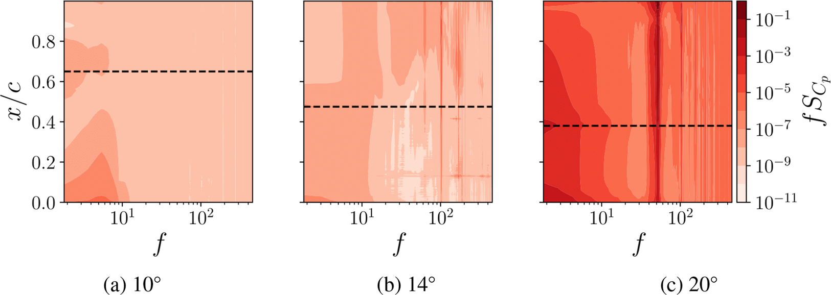
denoting the frequency. Figure 2 shows the pre-multiplied frequency spectrograms of the pressure signal
$ f $
denoting the frequency. Figure 2 shows the pre-multiplied frequency spectrograms of the pressure signal $ {fS}_{C_p} $
for the suction side of the blade at three different angles of attack corresponding to attached flow (
$ {fS}_{C_p} $
for the suction side of the blade at three different angles of attack corresponding to attached flow ( $ 10{}^{\circ} $
), the onset of separation (
$ 10{}^{\circ} $
), the onset of separation ( $ 14{}^{\circ} $
) and full separation (
$ 14{}^{\circ} $
) and full separation ( $ 20{}^{\circ} $
). As expected from Figure 1b, the energy levels increase with AoA. Below separation, low-frequency components (
$ 20{}^{\circ} $
). As expected from Figure 1b, the energy levels increase with AoA. Below separation, low-frequency components ( $ f\le 10 $
Hz), typically associated with the strong suction peak dynamics, dominate near the leading edge. At the onset of separation, a sharp frequency band centered at 100 Hz emerges from the spectrum. The frequency band width increases and its center increases with the angle of attack, as it reaches around 50 Hz at
$ f\le 10 $
Hz), typically associated with the strong suction peak dynamics, dominate near the leading edge. At the onset of separation, a sharp frequency band centered at 100 Hz emerges from the spectrum. The frequency band width increases and its center increases with the angle of attack, as it reaches around 50 Hz at $ 20{}^{\circ} $
. A Strouhal number based on the freestream velocity
$ 20{}^{\circ} $
. A Strouhal number based on the freestream velocity $ {U}_{\infty } $
and the shear layer height
$ {U}_{\infty } $
and the shear layer height $ h $
determined from the chord separation point and AoA yields a nearly constant value of
$ h $
determined from the chord separation point and AoA yields a nearly constant value of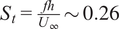 $ {S}_t=\frac{fh}{U_{\infty }}\sim 0.26 $
, which is consistent with the literature on 2D bluff bodies (Williamson, Reference Williamson1996).
$ {S}_t=\frac{fh}{U_{\infty }}\sim 0.26 $
, which is consistent with the literature on 2D bluff bodies (Williamson, Reference Williamson1996).
Pre-multiplied time spectrograms of $ {C}_p $
for AoA =
$ {C}_p $
for AoA = $ 10{}^{\circ} $
(a), AoA =
$ 10{}^{\circ} $
(a), AoA = $ 14{}^{\circ} $
(b), and AoA =
$ 14{}^{\circ} $
(b), and AoA = $ 20{}^{\circ} $
(c). Black dashed lines correspond to the location of the ISP.
$ 20{}^{\circ} $
(c). Black dashed lines correspond to the location of the ISP.
2.4. Wake characterization
This section introduces key performance indicators for the airfoil associated with the velocity field, referred to hereafter as the “ground truth.” Throughout the paper, the focus of the reconstruction will be the instantaneous streamwise velocity component, although a similar appproach could be carried out for the cross-stream component. Time-averaged as well as turbulent features are presented below.
2.4.1. Time-averaged wake
To characterize the mean features of the wake velocity deficit, defined as $ \Delta u\left(x,y\right)=\left({U}_{\infty }-\overline{u}\left(x,y\right)\right) $
, where
$ \Delta u\left(x,y\right)=\left({U}_{\infty }-\overline{u}\left(x,y\right)\right) $
, where $ \overline{.} $
represents a time average, the following two quantities are introduced:
$ \overline{.} $
represents a time average, the following two quantities are introduced:
-
• The wake width $ \delta $
is defined as the spanwise distance at which the time-averaged velocity deficit
$ \Delta u\left(x,y\right) $
reaches a fraction
$ \theta $
of the local maximum velocity deficit, such that
$ \Delta u\left(x,y=\delta \right)=\theta \Delta {u}_{\mathrm{max}}(x) $
. Although a common criterion in wind turbine wake modeling is to use
$ \theta =0.1 $
, a more conservative threshold
$ \theta =0.5 $
was used as it was found to provide a more robust estimate with respect to small-scale perturbations in the surrounding flow (Duda et al., Reference Duda, Uruba and Yanovych2021).
$ \delta $
is defined as the spanwise distance at which the time-averaged velocity deficit
$ \Delta u\left(x,y\right) $
reaches a fraction
$ \theta $
of the local maximum velocity deficit, such that
$ \Delta u\left(x,y=\delta \right)=\theta \Delta {u}_{\mathrm{max}}(x) $
. Although a common criterion in wind turbine wake modeling is to use
$ \theta =0.1 $
, a more conservative threshold
$ \theta =0.5 $
was used as it was found to provide a more robust estimate with respect to small-scale perturbations in the surrounding flow (Duda et al., Reference Duda, Uruba and Yanovych2021). -
• The wake deflection angle
$ \alpha $
is defined as the angle between the line corresponding to the locations of the maximum velocity deficit and the chord. It is computed as
$ \alpha =\arctan \left(\frac{y_{\mathrm{max}}-{y}_0}{x_{\mathrm{max}}-{x}_0}\right) $
, where (
$ {x}_{\mathrm{max}},{y}_{\mathrm{max}} $
) are the coordinates of the maximum velocity deficit and (
$ {x}_0,{y}_0 $
) the coordinates of the trailing edge.





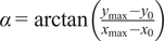


Figure 3 depicts the streamwise evolution of the wake width and the wake deflection angle for all angles of attack. Concerning the wake width, a general trend observed is that both $ \delta $
and
$ \delta $
and $ d\delta / dx $
increase with the angle of attack. For separated flow regimes, a specific trailing edge effect can be identified in the near wake (
$ d\delta / dx $
increase with the angle of attack. For separated flow regimes, a specific trailing edge effect can be identified in the near wake ( $ x/c\in \left[1;2\right] $
), as the width
$ x/c\in \left[1;2\right] $
), as the width $ \delta (x) $
first goes through a local minimum, then a local maximum, and
$ \delta (x) $
first goes through a local minimum, then a local maximum, and $ d\delta / dx $
jumps to higher values. At each angle of attack, the far wake evolution in the streamwise direction (
$ d\delta / dx $
jumps to higher values. At each angle of attack, the far wake evolution in the streamwise direction ( $ x>4c $
) can be characterized by a nearly constant growth rate, which increases with the angle of attack. Figure 3 also shows that the deflection angle
$ x>4c $
) can be characterized by a nearly constant growth rate, which increases with the angle of attack. Figure 3 also shows that the deflection angle $ \alpha $
increases with the angle of attack, with large variations in the near wake, and a quasi-linear increase in the far wake (it should be noted that the small oscillations observed there are an artefact of the computational mesh). The existence of a monotonic relationship thus makes it possible to infer the angle of attack from the deflection angle
$ \alpha $
increases with the angle of attack, with large variations in the near wake, and a quasi-linear increase in the far wake (it should be noted that the small oscillations observed there are an artefact of the computational mesh). The existence of a monotonic relationship thus makes it possible to infer the angle of attack from the deflection angle $ \alpha $
. The noisy behavior observed in the far wake profiles of both
$ \alpha $
. The noisy behavior observed in the far wake profiles of both $ \delta $
and
$ \delta $
and $ \alpha $
can be attributed to the mesh coarsening away from the airfoil.
$ \alpha $
can be attributed to the mesh coarsening away from the airfoil.
Streamwise evolution of the time-averaged wake width $ \delta (x)/c $
(a) and streamwise evolution of the time-averaged wake deflection angle
$ \delta (x)/c $
(a) and streamwise evolution of the time-averaged wake deflection angle $ \alpha $
(b). The profiles are shown for
$ \alpha $
(b). The profiles are shown for $ x/c\in \left[1;7\right] $
, where
$ x/c\in \left[1;7\right] $
, where $ x/c=1 $
corresponds to the streamwise location of the trailing edge.
$ x/c=1 $
corresponds to the streamwise location of the trailing edge.

2.4.2. Wake flow fluctuations
Since the reconstruction method aims to recover instantaneous velocity fields, attention is now turned to the time-dependent features of the wake. Snapshots of the instantaneous streamwise velocity field at an arbitrary time $ t=5 $
s are shown in the top row of Figure 4 at the same angles of attack as those in Figure 2. It is recalled that all fields shown in the paper are rotated by placing the airfoil at a
$ t=5 $
s are shown in the top row of Figure 4 at the same angles of attack as those in Figure 2. It is recalled that all fields shown in the paper are rotated by placing the airfoil at a $ 0{}^{\circ} $
incidence and aligning the flow at the correct angle with respect to the AoA). The vertical white dashed line at
$ 0{}^{\circ} $
incidence and aligning the flow at the correct angle with respect to the AoA). The vertical white dashed line at $ x/c=2 $
(near wake) corresponds to the section where pre-multiplied velocity spectra are extracted and shown on the bottom row of Figure 4.
$ x/c=2 $
(near wake) corresponds to the section where pre-multiplied velocity spectra are extracted and shown on the bottom row of Figure 4.
Snapshots of the normalized instantaneous streamwise velocity field $ u/{U}_{\infty } $
(top) and spectrograms of the pre-multiplied velocity spectra
$ u/{U}_{\infty } $
(top) and spectrograms of the pre-multiplied velocity spectra $ {fS}_u $
for the cases AoA
$ {fS}_u $
for the cases AoA $ =10{}^{\circ} $
(a), AoA
$ =10{}^{\circ} $
(a), AoA $ =14{}^{\circ} $
(b), and AoA
$ =14{}^{\circ} $
(b), and AoA $ =20{}^{\circ} $
(c). The vertical white dashed lines in the snapshots denote the
$ =20{}^{\circ} $
(c). The vertical white dashed lines in the snapshots denote the $ x/c=2 $
section where the spectrograms are computed. The horizontal yellow dashed lines in the spectrograms indicate the wake width.
$ x/c=2 $
section where the spectrograms are computed. The horizontal yellow dashed lines in the spectrograms indicate the wake width.

As observed for the pressure field, the total energy of the fluctuations increase with the angle of attack. The dominant frequencies observed in the pressure spectra in Figure 2 are also present in the pre-multiplied velocity spectra $ {fS}_u $
(100 and 50 Hz for AoA =
$ {fS}_u $
(100 and 50 Hz for AoA = $ 14{}^{\circ} $
and
$ 14{}^{\circ} $
and $ 20{}^{\circ} $
) and can be found to correspond to vortex shedding dynamics. However, several differences between pressure and velocity spectra can be noted, thus reflecting the nonlinear relationship between the pressure and velocity that the model needs to handle.
$ 20{}^{\circ} $
) and can be found to correspond to vortex shedding dynamics. However, several differences between pressure and velocity spectra can be noted, thus reflecting the nonlinear relationship between the pressure and velocity that the model needs to handle.
In this section, we have characterized the inputs and outputs of the model to be described later, namely the surface pressure and the streamwise velocity field. Both time-averaged and time-dependent flow properties, such as the characteristic wake width and orientation, as well as its spectral signature, will be used to assess the model performance.
3. Methodology
We now detail the estimation method for reconstructing the streamwise velocity field from a limited number of pressure measurements. We first describe how the sensor number and location are defined.
3.1. Sensor placement and number
Owing to cost and practical constraints, the number of sensors needs to be kept low in real-life applications. The sensor location is then critical because the information content is not uniformly distributed over the blade surface: regions such as the leading edge, trailing edge, or the intermittent separation zone carry substantially more information about the surrounding flow. Optimal sensor placement can be carried out by minimizing the uncertainties associated with the sensors, which can be measured by the information entropy (Papadimitriou, Reference Papadimitriou2004). Computing this minimum is a challenge that can be addressed by different approximations. Papadimitriou and Papadimitriou (Reference Papadimitriou and Papadimitriou2013) showed for a CFD application that the entropy can be approximated in terms of the gradients of the flow variables with respect to the flow parameters. Yoko and Juniper (Reference Yoko and Juniper2024) used adjoint-based optimization to compute the entropy minimum in an efficient manner. Bidar et al. (Reference Bidar, Anderson and Qin2024) did not solve the minimization problem directly, but determined the location of the sensors based on the variance of a chosen predicted variable. However, an ad hoc criterion needed to be implemented to avoid sensor clustering. Another way to avoid clustering is to use sparsity constraints for sensor placement optimization (see, for instance, Manohar et al., Reference Manohar, Brunton, Kutz and Brunton2018; Carter et al., Reference Carter, De Voogt, Soares and Ganapathisubramani2021; Hollenbeck et al., Reference Hollenbeck, Grandhi, Hansen and Pankonien2024; Bukowski et al., Reference Bukowski, Rennie and Gordeyev2025).
In the physical problem considered here, the turbulent flow dynamics to be reconstructed are conditioned by the development of a near-wall shear layer and a downstream wake, which are greatly influenced by the location of the separation point on the blade. Since different dynamics appear to be associated with different regions of the blade, we partitioned the blade into geometric clusters and implemented a variance-based, sparsity-promoting approach. In order to take into account the fluctuation level discrepancy between the different angles of attack, the optimization procedure was first carried out for each angle of attack. The sensor locations were then aggregated into a list. This list is then reduced to avoid sensor clustering: if the distance between two sensors is smaller than a given threshold value, only the sensor associated with the largest (absolute) variance is kept.
The procedure can be decomposed into three steps:
-
• The first step consists of clustering blade surface points into
$ {n}_c $
clusters based on their positions. The k-means clustering method is used (MacQueen, Reference MacQueen1967) and the number of clusters
$ {n}_c=25 $
is determined using the elbow method (Thorndike, Reference Thorndike1953). -
• In the second step, the optimal sensor locations are determined for each angle of attack: the wall-pressure variance is computed within each cluster, and the clusters are ranked according to their relative contribution to the total variance at this angle of attack. Given a variance threshold
$ {\sigma}_{\mathrm{thres}}^2 $
(expressed as a percentage of the total variance) to be captured, the minimal number of clusters
$ {p}_i $
necessary to capture this fraction is determined, and the corresponding clusters are selected. In each of these
$ {p}_i $
clusters, the sensor corresponding to the maximum variance is retained, the assumption being that the fluctuations of the point are representative of the fluctuations of the cluster. If two candidate sensors are found to be separated by less than
$ {d}_{min} $
, the one associated with the highest variance is kept in place, whereas the other is moved within its cluster at a distance
$ {d}_{min} $
. The minimum distance
$ {d}_{min} $
is taken to be
$ 0.01c $
and roughly corresponds to the pressure sensor spacing of Neunaber et al. (Reference Neunaber, Danbon, Soulier, Voisin, Guilmineau, Delpech, Courtine, Taymans and Braud2022)’s experiment. -
• The third step consists of concatenating the lists of sensor positions obtained for the total number of angles of attack
$ {N}_{\mathrm{AoA}} $
. At this last stage, if two sensors are found to be at a distance less than
$ {d}_{min} $
from each other, only the sensor associated with the highest variance—regardless of the angle of attack—is retained.


The procedure yields a total number of $ p\le {p}_i{N}_{\mathrm{AoA}} $
sensors. The sensor selection process is summarized in Table 1.
$ p\le {p}_i{N}_{\mathrm{AoA}} $
sensors. The sensor selection process is summarized in Table 1.
Methodology for selecting the wall pressure sensors based on maximizing the represented variance

Table 2 reports the correspondence between the target variance threshold $ {\sigma}_{\mathrm{thres}}^2 $
to be captured and the resulting number of sensors
$ {\sigma}_{\mathrm{thres}}^2 $
to be captured and the resulting number of sensors $ p $
required. The relationship between the variance threshold and the number of selected sensors is strongly nonlinear. At low threshold levels
$ p $
required. The relationship between the variance threshold and the number of selected sensors is strongly nonlinear. At low threshold levels $ \left(\le 30\%\right) $
, the number of sensors remains nearly constant or increases only marginally. This can be attributed to the dominance of the Leading Edge Maximum and Trailing Edge Maximum, whose strong fluctuations alone account for up to
$ \left(\le 30\%\right) $
, the number of sensors remains nearly constant or increases only marginally. This can be attributed to the dominance of the Leading Edge Maximum and Trailing Edge Maximum, whose strong fluctuations alone account for up to $ {\sigma}_{\mathrm{thres}}^2=30\% $
of the total variance. As the threshold increases, additional sensor positions are created—first in the leading and trailing edge regions, then in the separation region, associated with the ISP, and finally covering the surface of the airfoil, as shown in Figure 5. Based on the trade-off between reconstruction accuracy and the number of sensors, an optimal number of
$ {\sigma}_{\mathrm{thres}}^2=30\% $
of the total variance. As the threshold increases, additional sensor positions are created—first in the leading and trailing edge regions, then in the separation region, associated with the ISP, and finally covering the surface of the airfoil, as shown in Figure 5. Based on the trade-off between reconstruction accuracy and the number of sensors, an optimal number of $ p=7 $
sensors (hence representing
$ p=7 $
sensors (hence representing $ 55\% $
of wall pressure variance) was identified and will be used for most of the results presented below. This choice will be further detailed in Section 4.2.1.
$ 55\% $
of wall pressure variance) was identified and will be used for most of the results presented below. This choice will be further detailed in Section 4.2.1.
Number of sensors $ p $
as a function of the variance fraction
$ p $
as a function of the variance fraction $ {\sigma}_{\mathrm{thres}}^2 $

Sensor layouts selected with the variance-maximization strategy for different threshold levels.

3.2. The SNN-POD model
The SNN-POD model combines Proper Orthogonal Decomposition and the shallow decoder framework of Erichson et al. (Reference Erichson, Mathelin, Yao, Brunton, Mahoney and Kutz2020) to reconstruct the full velocity field from sparse wall pressure measurements taken over a range of angles of attack. The model is trained with snapshots corresponding to the set $ {I}_{train} $
of angles of attack of size
$ {I}_{train} $
of angles of attack of size $ {N}_{\mathrm{AoA}}=7 $
. For each angle of attack, a sequence of
$ {N}_{\mathrm{AoA}}=7 $
. For each angle of attack, a sequence of $ {N}_t $
snapshots is selected to constitute the training set, which therefore consists of
$ {N}_t $
snapshots is selected to constitute the training set, which therefore consists of $ {N}_t\times {N}_{\mathrm{AoA}} $
input/ouput couples, where each input is a pressure measurement vector of size
$ {N}_t\times {N}_{\mathrm{AoA}} $
input/ouput couples, where each input is a pressure measurement vector of size $ p $
, and each output is constituted by the snapshot of the velocity field of size
$ p $
, and each output is constituted by the snapshot of the velocity field of size $ {N}_s $
with only one velocity component (streamwise). Since the
$ {N}_s $
with only one velocity component (streamwise). Since the $ m $
-th snapshot, where
$ m $
-th snapshot, where $ 1\le m\le {N}_t{N}_{\mathrm{AoA}} $
, can be associated to a time
$ 1\le m\le {N}_t{N}_{\mathrm{AoA}} $
, can be associated to a time $ {t}_k $
and an angle of attack
$ {t}_k $
and an angle of attack $ {\mathrm{AoA}}_i $
, it will be referred to indifferently with the index
$ {\mathrm{AoA}}_i $
, it will be referred to indifferently with the index $ m $
or the tuple
$ m $
or the tuple $ \left(k,i\right) $
. The acquisition time resolution between snapshots was taken to be 0.05 convective time units (about 1.1 ms). We used
$ \left(k,i\right) $
. The acquisition time resolution between snapshots was taken to be 0.05 convective time units (about 1.1 ms). We used $ {N}_t=150 $
snapshots, so that the length of the training set is about
$ {N}_t=150 $
snapshots, so that the length of the training set is about $ 0.16 $
s, which corresponds to
$ 0.16 $
s, which corresponds to $ 8-16 $
vortex shedding cycles (defined using the vortex shedding frequencies observed in Figure 4), depending on the angle of attack. In order to train the model, the model inputs and outputs are standardized, where the mean and standard deviation are calculated over the entire training dataset (consisting of snapshots corresponding to the set
$ 8-16 $
vortex shedding cycles (defined using the vortex shedding frequencies observed in Figure 4), depending on the angle of attack. In order to train the model, the model inputs and outputs are standardized, where the mean and standard deviation are calculated over the entire training dataset (consisting of snapshots corresponding to the set $ {I}_{train} $
).
$ {I}_{train} $
).
The approach can be summarized as follows (see Figure 8): POD is first used to compress information to a low-order manifold, a dimensionality reduction process which is presented in Section 3.2.1. Due to the structure of the dataset, the low-order manifold can be further broken down into time-independent and time-dependent components. A model based on two shallow neural networks is then trained to learn the nonlinear mapping between the pressure measurements and the two components of the latent subspace (POD velocity amplitudes), the details of which are given in Section 3.2.2. The instantaneous flow field is then reconstructed from the temporal amplitudes estimated by the model and the spatial statistics of the training set.
3.2.1. Dimensionality reduction
Due to the high dimension of the full-order state to be reconstructed (see Section 2), each velocity field in the training set is first projected onto a low-dimensional linear subspace using Proper Orthogonal Decomposition (Lumley, Reference Lumley, Iaglom and Tatarski1967). Since $ {N}_t{N}_{\mathrm{AoA}}<{N}_s $
the method of snapshots (Sirovich, Reference Sirovich1987) is applied to the velocity fluctuation defined with respect to a mean
$ {N}_t{N}_{\mathrm{AoA}}<{N}_s $
the method of snapshots (Sirovich, Reference Sirovich1987) is applied to the velocity fluctuation defined with respect to a mean $ \left\langle u\right\rangle $
, where
$ \left\langle u\right\rangle $
, where $ \left\langle .\right\rangle $
refers to an average taken over all times and angles of attack. The method relies on the construction of a snapshot matrix
$ \left\langle .\right\rangle $
refers to an average taken over all times and angles of attack. The method relies on the construction of a snapshot matrix $ \mathbf{X} $
:
$ \mathbf{X} $
:
 $$ \mathbf{X}=\left[\begin{array}{cccc}\mid & \mid & & \mid \\ {}{\mathbf{u}}^1& {\mathbf{u}}^2& \dots & {\mathbf{u}}^{N_t{N}_{\mathrm{AoA}}}\\ {}\mid & \mid & & \mid \end{array}\right] $$
where each column of $ \mathbf{X}\in {\mathrm{\mathbb{R}}}^{N_s\times {N}_t{N}_{\mathrm{AoA}}} $
represents a velocity snapshot. It is to be noted that
$ \mathbf{X}\in {\mathrm{\mathbb{R}}}^{N_s\times {N}_t{N}_{\mathrm{AoA}}} $
represents a velocity snapshot. It is to be noted that $ {\mathbf{u}}^1 $
and
$ {\mathbf{u}}^1 $
and $ u\left(\mathbf{x},{t}_1,{\mathrm{AoA}}_1\right) $
will be considered as equivalent notations. Each snapshot (column) is normalized with respect to the full data set, that is over all angles of attack.
$ u\left(\mathbf{x},{t}_1,{\mathrm{AoA}}_1\right) $
will be considered as equivalent notations. Each snapshot (column) is normalized with respect to the full data set, that is over all angles of attack.
Singular value decomposition (SVD) of the snapshot matrix $ \mathbf{X} $
yields:
$ \mathbf{X} $
yields:
 $$ \mathbf{X}=\boldsymbol{\Phi} {\mathbf{SA}}^T $$
where
 $$ \boldsymbol{\Phi} =\left[{\phi}_1\hskip0.5em \dots \hskip0.5em {\phi}_{N_t{N}_{\mathrm{AoA}}}\right]\in {\mathrm{\mathbb{R}}}^{N_s\times {N}_t{N}_{\mathrm{AoA}}},\mathbf{A}=\left[\begin{array}{ccc}{\mathbf{a}}_1& \dots & {\mathbf{a}}_{N_t{N}_{\mathrm{AoA}}}\end{array}\right]\in {\mathrm{\mathbb{R}}}^{N_t{N}_{\mathrm{AoA}}\times {N}_t{N}_{\mathrm{AoA}}}, $$
 $$ \mathbf{S}=\operatorname{diag}\left({\lambda}_1^{1/2},\dots, {\lambda}_{N_t{N}_{\mathrm{AoA}}}^{1/2}\right)\in {\mathrm{\mathbb{R}}}^{N_t{N}_{\mathrm{AoA}}\times {N}_t{N}_{\mathrm{AoA}}}, $$
with $ \mathbf{S} $
the diagonal matrix of singular values ranked by magnitude,
$ \mathbf{S} $
the diagonal matrix of singular values ranked by magnitude, $ \boldsymbol{\Phi} $
the matrix of linear POD modes and
$ \boldsymbol{\Phi} $
the matrix of linear POD modes and $ \mathbf{A} $
the matrix of POD time coefficients. Each POD mode
$ \mathbf{A} $
the matrix of POD time coefficients. Each POD mode $ {\phi}_n\left(\mathbf{x}\right) $
,
$ {\phi}_n\left(\mathbf{x}\right) $
, $ n=1,\dots {N}_t{N}_{\mathrm{AoA}}, $
satisfies the orthonormality condition as well as each amplitude vector
$ n=1,\dots {N}_t{N}_{\mathrm{AoA}}, $
satisfies the orthonormality condition as well as each amplitude vector $ {\mathbf{a}}_n $
. The value
$ {\mathbf{a}}_n $
. The value $ {\lambda}_n $
represents the contribution of the
$ {\lambda}_n $
represents the contribution of the $ n $
th mode to the variance of the velocity field so that the singular value
$ n $
th mode to the variance of the velocity field so that the singular value $ {\lambda}_n^{1/2} $
represents the global mode intensity in physical space. Each streamwise velocity field of the training set can thus be expressed at any angle of attack
$ {\lambda}_n^{1/2} $
represents the global mode intensity in physical space. Each streamwise velocity field of the training set can thus be expressed at any angle of attack $ {\mathrm{AoA}}_i $
with a unique POD basis:
$ {\mathrm{AoA}}_i $
with a unique POD basis:
 $$ u\left(\mathbf{x},{t}_k,{\mathrm{AoA}}_i\right)=\left\langle u\left(\mathbf{x}\right)\right\rangle +{u}^{\prime}\left(\mathbf{x},{t}_k,{\mathrm{AoA}}_i\right)\hskip0.22em \mathrm{where}\hskip0.22em {u}^{\prime}\left(\mathbf{x},{t}_k,{\mathrm{AoA}}_i\right)=\sum \limits_{n=1}^{N_t{N}_{\mathrm{AoA}}}{\lambda}_n^{1/2}{a}_n^{k,i}{\phi}_n\left(\mathbf{x}\right) $$
Figure 6 shows the singular values $ {\lambda}_i^{1/2} $
for training sets of different lengths
$ {\lambda}_i^{1/2} $
for training sets of different lengths $ {N}_t{N}_{\mathrm{AoA}} $
. It can be seen that convergence is reached for training set lengths
$ {N}_t{N}_{\mathrm{AoA}} $
. It can be seen that convergence is reached for training set lengths $ {N}_t\ge 50 $
and that more than 99% of the total variance is captured by the first 50 POD modes. Figure 7 shows the first six most energetic POD spatial modes
$ {N}_t\ge 50 $
and that more than 99% of the total variance is captured by the first 50 POD modes. Figure 7 shows the first six most energetic POD spatial modes $ {\phi}_n\left(\mathbf{x}\right) $
,
$ {\phi}_n\left(\mathbf{x}\right) $
, $ n=1,\dots 6 $
and their amplitudes
$ n=1,\dots 6 $
and their amplitudes $ {a}_n $
which are plotted separately for each angle of attack. The six spatial modes can be split into two groups: on the one hand, modes 1, 2, 3, and 5 are important in the shear layer and separation zone while on the other hand, modes 4 and 6 are dominant in the wake. The energy level of the latter modes is similar, and their shape is consistent with a pair of vortex shedding modes. It can be further observed that the amplitudes of the modes in the first group are characterized by non-zero time-averaged values, which are distinct for each angle of attack, indicating that they correspond to time-independent field deformation due to the angle of attack. In contrast, the time-average of the amplitudes in the second group is zero, and the amplitudes are characterized by large oscillations which increase with separation. A criterion can thus be defined to determine whether a POD mode
$ {a}_n $
which are plotted separately for each angle of attack. The six spatial modes can be split into two groups: on the one hand, modes 1, 2, 3, and 5 are important in the shear layer and separation zone while on the other hand, modes 4 and 6 are dominant in the wake. The energy level of the latter modes is similar, and their shape is consistent with a pair of vortex shedding modes. It can be further observed that the amplitudes of the modes in the first group are characterized by non-zero time-averaged values, which are distinct for each angle of attack, indicating that they correspond to time-independent field deformation due to the angle of attack. In contrast, the time-average of the amplitudes in the second group is zero, and the amplitudes are characterized by large oscillations which increase with separation. A criterion can thus be defined to determine whether a POD mode $ {a}_n $
is steady or unsteady by comparing its time average for each angle of attack
$ {a}_n $
is steady or unsteady by comparing its time average for each angle of attack $ {\overline{a}}_n\left(\mathrm{AoA}\right) $
with the amplitude of its variations. Specifically, a mode will be considered to be steady (resp. unsteady) if:
$ {\overline{a}}_n\left(\mathrm{AoA}\right) $
with the amplitude of its variations. Specifically, a mode will be considered to be steady (resp. unsteady) if:
 $$ \underset{\mathrm{AoA}}{\max}\mid \underset{N_t}{\max}\;{\mathbf{a}}_n-\underset{N_t}{\min}\;{\mathbf{a}}_n\mid >\underset{\mathrm{AoA}}{\max}\mid \overline{{\mathbf{a}}_n}\mid . $$
This makes it possible to split POD modes into steady and unsteady modes, which will be indexed respectively with the suffixes $ st $
and
$ st $
and $ un $
. A discussion on the relevance and robustness of this splitting is provided in Section 4.2.2.
$ un $
. A discussion on the relevance and robustness of this splitting is provided in Section 4.2.2.
Singular values $ {\lambda}_i^{1/2} $
obtained from the POD of training datasets of varying sizes, the red vertical dashed line indicates the POD truncation at
$ {\lambda}_i^{1/2} $
obtained from the POD of training datasets of varying sizes, the red vertical dashed line indicates the POD truncation at $ r=50 $
.
$ r=50 $
.

Sets of POD modes $ {\boldsymbol{\Phi}}_{\mathbf{i}} $
(top) and their associated POD coefficients
$ {\boldsymbol{\Phi}}_{\mathbf{i}} $
(top) and their associated POD coefficients $ {\mathbf{a}}_{\mathbf{i}} $
(bottom) for
$ {\mathbf{a}}_{\mathbf{i}} $
(bottom) for $ i=1,\dots, 6 $
(a,…,f). Their contribution to the total variance is denoted in parentheses in captions.
$ i=1,\dots, 6 $
(a,…,f). Their contribution to the total variance is denoted in parentheses in captions.

Schematic representation of the SNN-POD reconstruction framework. Steady (denoted with the $ st $
subscript) and unsteady (denoted with the
$ st $
subscript) and unsteady (denoted with the $ un $
subscript) modes resulting from the Proper Orthogonal Decomposition of the training dataset are treated separately by the SNN-POD. Two Shallow Neural Networks (SNN) learn the mapping between the sparse wall pressure measurements and the steady and unsteady POD coefficients using an energy-weighted loss. The high-dimensional flow field is then recovered from the POD training basis
$ un $
subscript) modes resulting from the Proper Orthogonal Decomposition of the training dataset are treated separately by the SNN-POD. Two Shallow Neural Networks (SNN) learn the mapping between the sparse wall pressure measurements and the steady and unsteady POD coefficients using an energy-weighted loss. The high-dimensional flow field is then recovered from the POD training basis $ \mathtt{\varPhi} $
and estimated model amplitudes.
$ \mathtt{\varPhi} $
and estimated model amplitudes.

3.2.2. Construction of the model
Given an input vector of pressure measurements of size $ p $
, the model learns the projection onto the POD basis by estimating the
$ p $
, the model learns the projection onto the POD basis by estimating the $ r $
most energetic POD coefficients
$ r $
most energetic POD coefficients $ {\hat{a}}_i $
, which are then combined to reconstruct the flow field of size
$ {\hat{a}}_i $
, which are then combined to reconstruct the flow field of size $ {N}_s $
using:
$ {N}_s $
using:
 $$ \hat{u}\left(\mathbf{x}\right)=\left\langle u\left(\mathbf{x}\right)\right\rangle +\sum \limits_{1\le n\le r}{\lambda}_n^{1/2}{\hat{a}}_n{\phi}_n\left(\mathbf{x}\right) $$
where $ \left\langle u\left(\mathbf{x}\right)\right\rangle $
,
$ \left\langle u\left(\mathbf{x}\right)\right\rangle $
, $ {\lambda}_n $
and
$ {\lambda}_n $
and $ {\phi}_n $
are determined from the training set. A preliminary analysis conducted on a single AoA configuration (not shown) indicated that increasing the number of POD modes generally enhances the reconstruction accuracy; however, the improvement becomes marginal for
$ {\phi}_n $
are determined from the training set. A preliminary analysis conducted on a single AoA configuration (not shown) indicated that increasing the number of POD modes generally enhances the reconstruction accuracy; however, the improvement becomes marginal for $ r\ge 50 $
retained modes. For this reason, the value of
$ r\ge 50 $
retained modes. For this reason, the value of $ r=50 $
POD modes, corresponding to a compression ratio of
$ r=50 $
POD modes, corresponding to a compression ratio of $ 96.75\% $
, was chosen for the present study.
$ 96.75\% $
, was chosen for the present study.
The amplitudes to be learnt $ {\hat{a}}_n $
are split into two output vectors consisting of steady and unsteady modes—according to the previous section—which are independently learnt by two networks based on the shallow decoder architecture outlined in Erichson et al. (Reference Erichson, Mathelin, Yao, Brunton, Mahoney and Kutz2020), which we first briefly review. A Shallow Neural Network (SNN) is a neural network consisting of
$ {\hat{a}}_n $
are split into two output vectors consisting of steady and unsteady modes—according to the previous section—which are independently learnt by two networks based on the shallow decoder architecture outlined in Erichson et al. (Reference Erichson, Mathelin, Yao, Brunton, Mahoney and Kutz2020), which we first briefly review. A Shallow Neural Network (SNN) is a neural network consisting of $ L $
fully-connected hidden layers (with
$ L $
fully-connected hidden layers (with $ L\le 3 $
in general). Given an input
$ L\le 3 $
in general). Given an input $ \mathbf{s} $
, the output of the model is defined as
$ \mathbf{s} $
, the output of the model is defined as
 $$ \mathcal{F}\left(\mathbf{s};\mathbf{w}\right)={\mathbf{w}}^{\mathbf{L}}g\left({\mathbf{w}}^{\mathbf{L}-\mathbf{1}}\dots g\left({\mathbf{w}}^{\mathbf{1}}\mathbf{s}\right)\right), $$
where $ g $
is a non-linear activation function and
$ g $
is a non-linear activation function and $ \mathbf{w} $
the set of weights matrices. Here
$ \mathbf{w} $
the set of weights matrices. Here $ L=3 $
and
$ L=3 $
and $ g $
is the ReLu function. The model used in the present study relies on two SNNs with identical architectures. The robustness of each network is improved by the addition of a dropout with a drop ratio of
$ g $
is the ReLu function. The model used in the present study relies on two SNNs with identical architectures. The robustness of each network is improved by the addition of a dropout with a drop ratio of $ 10\% $
. An Adaptative Moment Estimation (ADAM) optimizer is used along with a regularization method (weight decay) to prevent overfitting. Training batches are shuffled, and the mini-batch size is set to
$ 10\% $
. An Adaptative Moment Estimation (ADAM) optimizer is used along with a regularization method (weight decay) to prevent overfitting. Training batches are shuffled, and the mini-batch size is set to $ 128 $
. Both networks are trained over 4000 epochs but training may be shortened by early stopping, which acts as a regularizer to avoid overfitting (Goodfellow et al., Reference Goodfellow, Bengio and Courville2016). In practice early stopping is applied if the error on the testing dataset does not reduce over 100 epochs. The choice of the optimal set of hyperparameters (i.e. parameters external to the learning process which are directly learnt within estimators) is determined by using Optuna hyperparameter optimization software framework based on Bayesian optimization (Akiba et al., Reference Akiba, Sano, Yanase, Ohta and & Koyama2019). The list of optimized hyperparameters and their associated values is given in Table 3.
$ 128 $
. Both networks are trained over 4000 epochs but training may be shortened by early stopping, which acts as a regularizer to avoid overfitting (Goodfellow et al., Reference Goodfellow, Bengio and Courville2016). In practice early stopping is applied if the error on the testing dataset does not reduce over 100 epochs. The choice of the optimal set of hyperparameters (i.e. parameters external to the learning process which are directly learnt within estimators) is determined by using Optuna hyperparameter optimization software framework based on Bayesian optimization (Akiba et al., Reference Akiba, Sano, Yanase, Ohta and & Koyama2019). The list of optimized hyperparameters and their associated values is given in Table 3.
List of the tuned hyperparameters and their optimal values for each SNN. $ p $
refers to the number of sensors or inputs (results shown correspond to
$ p $
refers to the number of sensors or inputs (results shown correspond to $ p=7 $
) and
$ p=7 $
) and $ r $
is the number of POD modes (outputs) to be reconstructed by an SNN (results shown correspond to
$ r $
is the number of POD modes (outputs) to be reconstructed by an SNN (results shown correspond to $ {r}_{st}=6 $
and
$ {r}_{st}=6 $
and $ {r}_{un}=544 $
respectively for the steady-mode and the unsteady-mode SNN)
$ {r}_{un}=544 $
respectively for the steady-mode and the unsteady-mode SNN)

Each SNN is trained to minimize the $ {L}_2 $
-norm of the error between the reduced state and its estimation, weighted by the associated eigenvalue (contribution of the mode to the variance), so that the loss is given by:
$ {L}_2 $
-norm of the error between the reduced state and its estimation, weighted by the associated eigenvalue (contribution of the mode to the variance), so that the loss is given by:
 $$ {\displaystyle \begin{array}{c}{\mathrm{\mathcal{L}}}_{POD}=\sum \limits_{1\le n\le r}{\lambda}_n\sum \limits_{1\le m\le {N}_t{N}_{\mathrm{AoA}}}\parallel {a}_n^m-{\hat{a}}_n^m{\parallel}^2={\left\Vert \mathbf{S}\left[{\mathbf{A}}^k-\mathcal{F}\left({\mathbf{s}}^k;\mathbf{w}\right)\right]\right\Vert}_2^2\end{array}} $$
The application of $ S $
means that the error between the normalized amplitude of mode
$ S $
means that the error between the normalized amplitude of mode $ n $
and its prediction is scaled by the mode intensity
$ n $
and its prediction is scaled by the mode intensity $ {\lambda}_n^{1/2} $
, so that the loss corresponds to the global error in physical space. The mode intensities
$ {\lambda}_n^{1/2} $
, so that the loss corresponds to the global error in physical space. The mode intensities $ {\lambda}_n^{1/2} $
are not predicted by the model, but are directly extracted from the POD decomposition of the training dataset.
$ {\lambda}_n^{1/2} $
are not predicted by the model, but are directly extracted from the POD decomposition of the training dataset.
The test set consists of unseen snapshots for angles of attack, both within and outside $ {I}_{train} $
. Specifically, three new angles were considered:
$ {I}_{train} $
. Specifically, three new angles were considered: $ 15.5{}^{\circ},17{}^{\circ},19{}^{\circ} $
so the total number of angles in the test set is
$ 15.5{}^{\circ},17{}^{\circ},19{}^{\circ} $
so the total number of angles in the test set is $ {N}_{\mathrm{AoA}}^{test}=10 $
. For each AoA
$ {N}_{\mathrm{AoA}}^{test}=10 $
. For each AoA $ \in {I}_{test} $
a sequence of
$ \in {I}_{test} $
a sequence of $ {N}_t^{test}=50 $
snapshots were selected to constitute the test set presented in the paper. Results did not change significantly for larger numbers or random selections of snapshots.
$ {N}_t^{test}=50 $
snapshots were selected to constitute the test set presented in the paper. Results did not change significantly for larger numbers or random selections of snapshots.
To evaluate the model accuracy on the test set, the following metrics were used:
-
• the normalized mean-square error (MSE)
$ {E}_{test} $
, given by:

 $$ {E}_{test}=\frac{1}{N_{\mathrm{AoA}}^{test}{N}_t^{test}}\sum \limits_{\begin{array}{c}1\le i\le {N}_{\mathrm{AoA}}^{test}\\ {}1\le k\le {N}_t^{test}\end{array}}\frac{{\left\Vert {\mathbf{u}}^{k,i}-{\hat{\mathbf{u}}}^{k,i}\right\Vert}_2}{{\left\Vert {\mathbf{u}}^{k,i}\right\Vert}_2} $$
-
• the fluctuation error
$ {\varepsilon}_{test} $
, based on the fluctuating part of the velocity field
$ {u}^{\prime } $
(with respect to the average taken over the training set), defined as(6)By construction, the fluctuation error is larger than the MSE. It is also independent of the fluctuation to mean ratio, which can bias the MSE.
$$ {\varepsilon}_{test}=\frac{1}{N_{\mathrm{AoA}}^{test}{N}_t^{test}}\sum \limits_{\begin{array}{c}1\le i\le {N}_{\mathrm{AoA}}^{test}\\ {}1\le k\le {N}_t^{test}\end{array}}\frac{{\left\Vert {{\mathbf{u}}^{\prime}}^{k,i}-{\hat{{\mathbf{u}}^{\prime}}}^{k,i}\right\Vert}_2}{{\left\Vert {{\mathbf{u}}^{\prime}}^{k,i}\right\Vert}_2} $$
-
• the projection error
$ {\varepsilon}_{test}^{\boldsymbol{\Phi}} $
measures the relative difference between the reconstruction and the projection of the ground truth velocity field onto the POD basis of
$ r $
modes:


 $$ {\varepsilon}_{test}^{\boldsymbol{\Phi}}=\frac{1}{N_{\mathrm{AoA}}^{test}{N}_t^{test}}\sum \limits_{\begin{array}{c}1\le i\le {N}_{\mathrm{AoA}}^{test}\\ {}1\le k\le {N}_t^{test}\end{array}}\frac{{\left\Vert {{\mathbf{u}}^{\prime}}_{\boldsymbol{\Phi}}^{k,i}-{\hat{{\mathbf{u}}^{\prime}}}^{k,i}\right\Vert}_2}{{\left\Vert {{\mathbf{u}}^{\prime}}_{\boldsymbol{\Phi}}^{k,i}\right\Vert}_2}. $$
where $ {{\mathbf{u}}^{\prime}}_{\boldsymbol{\Phi}}^{k,i}={\sum}_{1\le n\le r}{a}_n^{k,i}{\Phi}_n $
is the projection of the ground truth field onto the POD basis of the training set, which represents the best approximation achievable by the SNN-POD. Comparing the fluctuation and the projection error, therefore, provides a measure of the suitability of the POD training basis.
$ {{\mathbf{u}}^{\prime}}_{\boldsymbol{\Phi}}^{k,i}={\sum}_{1\le n\le r}{a}_n^{k,i}{\Phi}_n $
is the projection of the ground truth field onto the POD basis of the training set, which represents the best approximation achievable by the SNN-POD. Comparing the fluctuation and the projection error, therefore, provides a measure of the suitability of the POD training basis.
4. Results
In this section, the performance of the SNN-POD model trained on the full range of angles of attack is evaluated on the test set. The robustness of the model is then examined through a sensitivity analysis (Section 4.2.1) of the sensor placement strategy described in Section 3.1, followed by a study of the influence of the modal splitting approach (Section 4.2.2) on the model performance. Finally, Section 4.3 describes how combining SNN-POD models trained on different subsets of angles of attack can locally improve the reconstruction.
4.1. Evaluation of SNN-POD
This section evaluates the ability of the SNN-POD model to estimate both the POD coefficients and the instantaneous velocity field $ u $
from the URANS simulations, denoted thereafter as the “ground truth.” As mentioned earlier, the test set includes angles sampled during training as well as angles that are not part of the original discretization (interpolated angles). Figures 9–
12 compare characteristic features of the true and reconstructed flow fields for three sampled
$ u $
from the URANS simulations, denoted thereafter as the “ground truth.” As mentioned earlier, the test set includes angles sampled during training as well as angles that are not part of the original discretization (interpolated angles). Figures 9–
12 compare characteristic features of the true and reconstructed flow fields for three sampled $ \left(10{}^{\circ},15{}^{\circ},20{}^{\circ}\right) $
and three interpolated angles
$ \left(10{}^{\circ},15{}^{\circ},20{}^{\circ}\right) $
and three interpolated angles $ \left(15.5{}^{\circ},17{}^{\circ},19{}^{\circ}\right) $
. Each column corresponds to an angle of attack. Figures 9 and 11 provide a comparison of a ground truth snapshot (top row) with its reconstruction (bottom row) for sampled and interpolated angles, respectively. In all cases, a very good agreement is observed for the main features of the flow, although some slight differences are noticeable for the interpolated angles, particularly in the far wake.
$ \left(15.5{}^{\circ},17{}^{\circ},19{}^{\circ}\right) $
. Each column corresponds to an angle of attack. Figures 9 and 11 provide a comparison of a ground truth snapshot (top row) with its reconstruction (bottom row) for sampled and interpolated angles, respectively. In all cases, a very good agreement is observed for the main features of the flow, although some slight differences are noticeable for the interpolated angles, particularly in the far wake.
Comparison of streamwise velocity $ u\left(\mathbf{x},{t}_s\right)/{U}_{\infty } $
contours at snapshot
$ u\left(\mathbf{x},{t}_s\right)/{U}_{\infty } $
contours at snapshot $ {t}_s=150 $
s of the ground truth obtained from URANS (left) and its SNN-POD estimation (right) for three AoA:
$ {t}_s=150 $
s of the ground truth obtained from URANS (left) and its SNN-POD estimation (right) for three AoA: $ 10{}^{\circ} $
(left),
$ 10{}^{\circ} $
(left), $ 15{}^{\circ} $
(center) and
$ 15{}^{\circ} $
(center) and $ 20{}^{\circ} $
(right). The locations of the
$ 20{}^{\circ} $
(right). The locations of the $ p=7 $
pressure sensors on the blade are indicated with blue markers.
$ p=7 $
pressure sensors on the blade are indicated with blue markers.

Top plots denote the wake widths and wake deflection angles comparison between the ground truth and the estimation for three AoA: $ 10{}^{\circ} $
(left),
$ 10{}^{\circ} $
(left), $ 15{}^{\circ} $
(center) and
$ 15{}^{\circ} $
(center) and $ 20{}^{\circ} $
(right). Bottom plots correspond to the spectrograms of the pre-multiplied velocity spectra
$ 20{}^{\circ} $
(right). Bottom plots correspond to the spectrograms of the pre-multiplied velocity spectra $ {fS}_u $
of the ground truth (filled contours in blue shades) and SNN-POD estimation (red contour lines) at the
$ {fS}_u $
of the ground truth (filled contours in blue shades) and SNN-POD estimation (red contour lines) at the $ x/c=2 $
section. The same logarithmic colormap is applied to both spectrograms.
$ x/c=2 $
section. The same logarithmic colormap is applied to both spectrograms.

Comparison of streamwise velocity $ u\left(\mathbf{x},{t}_s\right) $
contours at snapshot
$ u\left(\mathbf{x},{t}_s\right) $
contours at snapshot $ {t}_s=150 $
s of the ground truth obtained from URANS (first plot from left to right) and its SNN-POD estimation (second plot) for three interpolated AoA:
$ {t}_s=150 $
s of the ground truth obtained from URANS (first plot from left to right) and its SNN-POD estimation (second plot) for three interpolated AoA: $ 15.5{}^{\circ} $
(left),
$ 15.5{}^{\circ} $
(left), $ 17{}^{\circ} $
(center) and
$ 17{}^{\circ} $
(center) and $ 19{}^{\circ} $
(right). The locations of the
$ 19{}^{\circ} $
(right). The locations of the $ p=7 $
pressure sensors on the blade are indicated with blue markers.
$ p=7 $
pressure sensors on the blade are indicated with blue markers.

Wake widths and wake deflection angles comparison between the ground truth and the estimation (top) for three unseen AoA: $ 15.5{}^{\circ} $
(left),
$ 15.5{}^{\circ} $
(left), $ 17{}^{\circ} $
(center) and
$ 17{}^{\circ} $
(center) and $ 19{}^{\circ} $
(right). Bottom plots correspond to the spectrograms of the pre-multiplied velocity spectra
$ 19{}^{\circ} $
(right). Bottom plots correspond to the spectrograms of the pre-multiplied velocity spectra $ {fS}_u $
of the ground truth (filled contours in blue shades) and SNN-POD estimation (red contour lines) at the
$ {fS}_u $
of the ground truth (filled contours in blue shades) and SNN-POD estimation (red contour lines) at the $ x/c=2 $
section. The same logarithmic colormap is applied for both spectrograms.
$ x/c=2 $
section. The same logarithmic colormap is applied for both spectrograms.

A more quantitative assessment can be made by examining the top rows of Figures 10 and 12, which show the average wake width and deflection angles. The wake width is well recovered for the sampled angles (Figure 10). For the interpolated angles (Figure 12), the wake width is characterized by small oscillations for $ x/c>1.5 $
and tends to be overpredicted for the two higher angles, although the growth rate
$ x/c>1.5 $
and tends to be overpredicted for the two higher angles, although the growth rate $ d\delta / dx $
generally appears to be correct and the maximum observed error is less than 15%. Moreover, the deflection angle is well recovered for both sampled and interpolated angles, which shows that the model is able to identify the angle of attack of the configuration from a single set of pressure measurements. This result is particularly important in the context of wind energy, where the estimation of instantaneous wind loads is directly linked to the determination of the AoA.
$ d\delta / dx $
generally appears to be correct and the maximum observed error is less than 15%. Moreover, the deflection angle is well recovered for both sampled and interpolated angles, which shows that the model is able to identify the angle of attack of the configuration from a single set of pressure measurements. This result is particularly important in the context of wind energy, where the estimation of instantaneous wind loads is directly linked to the determination of the AoA.
The bottom lines of Figures 10 and 12 compare the time spectra of the true and estimated velocity fields for sampled and interpolated angles, respectively. For all AoAs, the energy levels are accurately predicted, and the characteristic frequencies associated with flow separation are also well captured. The largest discrepancies in the spectrograms are observed for the attached flow case ( $ 10{}^{\circ} $
), where wake turbulence is low in energy. The model is able to predict the frequency shift observed for both sampled and interpolated angles and reproduces the complexity of the spectra, although unsurprisingly, the agreement is closer for sampled angles.
$ 10{}^{\circ} $
), where wake turbulence is low in energy. The model is able to predict the frequency shift observed for both sampled and interpolated angles and reproduces the complexity of the spectra, although unsurprisingly, the agreement is closer for sampled angles.
A more direct evaluation of the model performance is provided by Figure 13, which compares the estimated POD coefficients with their true values at all angles. Again, snapshots have been organized by increasing angle of attack and in chronological order so that the dynamics of the reconstruction can be evaluated, although no time dependence is accounted for in the model. Interpolated angles are indicated by green shaded regions. As noted in Figure 7, strong non-monotonic variations are observed in the amplitudes of the first three modes around AoA $ =14{}^{\circ} $
, while the evolution appears to be more gradual for AoA
$ =14{}^{\circ} $
, while the evolution appears to be more gradual for AoA $ \ge 15{}^{\circ} $
. Average errors for each mode and angle of attack are reported in Table 4. The amplitudes appear to be correctly predicted for almost all angles of attack, in particular, the first two modes. The exception is AoA
$ \ge 15{}^{\circ} $
. Average errors for each mode and angle of attack are reported in Table 4. The amplitudes appear to be correctly predicted for almost all angles of attack, in particular, the first two modes. The exception is AoA $ =15.5{}^{\circ} $
, where errors between 250% and 120% are reported for modes 3 to 6. Interestingly, the true value of mode 3 at this angle does not correspond to a direct interpolation of the angles AoA
$ =15.5{}^{\circ} $
, where errors between 250% and 120% are reported for modes 3 to 6. Interestingly, the true value of mode 3 at this angle does not correspond to a direct interpolation of the angles AoA $ =15{}^{\circ} $
and AoA
$ =15{}^{\circ} $
and AoA $ =16{}^{\circ} $
, a trend which the model captures but overpredicts.
$ =16{}^{\circ} $
, a trend which the model captures but overpredicts.
Comparison between the true POD amplitudes $ {a}_i $
(black lines) and the model estimates
$ {a}_i $
(black lines) and the model estimates $ {\hat{a}}_i $
(SNN-POD estimation red dashed lines) on the test dataset, with
$ {\hat{a}}_i $
(SNN-POD estimation red dashed lines) on the test dataset, with $ i=\mathrm{1,2,3,4,5,6} $
(a,b,c,d,e,f respectively). The test snapshots are organized into chronological time and sorted by angles of attack-angles of attack seen during training are displayed on a white background, and those not seen are highlighted with light green backgrounds.
$ i=\mathrm{1,2,3,4,5,6} $
(a,b,c,d,e,f respectively). The test snapshots are organized into chronological time and sorted by angles of attack-angles of attack seen during training are displayed on a white background, and those not seen are highlighted with light green backgrounds.

Mode reconstruction testing errors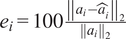 $ {e}_i=100\frac{{\left\Vert {a}_i-{\hat{a}}_i\right\Vert}_2}{{\left\Vert {a}_i\right\Vert}_2} $
per AoA for sampled and interpolated angles on the first six modes
$ {e}_i=100\frac{{\left\Vert {a}_i-{\hat{a}}_i\right\Vert}_2}{{\left\Vert {a}_i\right\Vert}_2} $
per AoA for sampled and interpolated angles on the first six modes
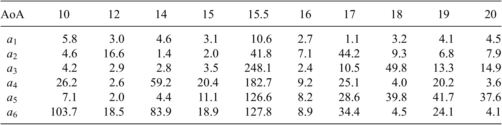
The mean, fluctuation, and projected fluctuation errors are defined in Section 3.2.2 are computed individually for each angle of attack of the test dataset and shown in Figure 14. As expected, errors are higher for interpolated AoA than for sampled AoA. Nonetheless, the mean reconstruction error remains below $ 6.6\% $
(maximum observed for
$ 6.6\% $
(maximum observed for $ 17{}^{\circ} $
), while the largest fluctuation errors
$ 17{}^{\circ} $
), while the largest fluctuation errors $ {\varepsilon}_{\mathrm{test}} $
are about
$ {\varepsilon}_{\mathrm{test}} $
are about $ 30\% $
for
$ 30\% $
for $ 15.5{}^{\circ} $
and
$ 15.5{}^{\circ} $
and $ 17{}^{\circ} $
, and reach about
$ 17{}^{\circ} $
, and reach about $ 23\% $
for
$ 23\% $
for $ 19{}^{\circ} $
. The projection error is essentially equal to the fluctuation error for sampled angles but about 25% lower for interpolated angles, a fraction that tends to decrease as the AoA increases (
$ 19{}^{\circ} $
. The projection error is essentially equal to the fluctuation error for sampled angles but about 25% lower for interpolated angles, a fraction that tends to decrease as the AoA increases ( $ 25\% $
for
$ 25\% $
for $ 15.5{}^{\circ} $
and
$ 15.5{}^{\circ} $
and $ 17{}^{\circ} $
, and under
$ 17{}^{\circ} $
, and under $ 20\% $
for
$ 20\% $
for $ 19{}^{\circ} $
). Overall, this points to a moderate influence of the POD basis on the model error. It can be noted that the projection error is largest for
$ 19{}^{\circ} $
). Overall, this points to a moderate influence of the POD basis on the model error. It can be noted that the projection error is largest for $ 15.5{}^{\circ} $
, despite the finer AoA resolution in that range. This suggests that significant changes occur in this range of angle of attack, which is also consistent with the higher errors observed at the angles
$ 15.5{}^{\circ} $
, despite the finer AoA resolution in that range. This suggests that significant changes occur in this range of angle of attack, which is also consistent with the higher errors observed at the angles $ 14{}^{\circ} $
,
$ 14{}^{\circ} $
, $ 15{}^{\circ} $
, and to a lesser extent
$ 15{}^{\circ} $
, and to a lesser extent $ 16{}^{\circ} $
. This point will be further discussed in Section 4.3.
$ 16{}^{\circ} $
. This point will be further discussed in Section 4.3.
Testing mean error $ {E}_{test} $
, fluctuating error
$ {E}_{test} $
, fluctuating error $ {\varepsilon}_{test} $
and projected fluctuating error
$ {\varepsilon}_{test} $
and projected fluctuating error $ {\varepsilon}_{test}^{\mathtt{\varPhi}} $
on testing datasets for each AoA configuration. The three interpolated AoA
$ {\varepsilon}_{test}^{\mathtt{\varPhi}} $
on testing datasets for each AoA configuration. The three interpolated AoA $ \left\{15.5{}^{\circ};17{}^{\circ};19{}^{\circ}\right\} $
are highlighted in green.
$ \left\{15.5{}^{\circ};17{}^{\circ};19{}^{\circ}\right\} $
are highlighted in green.

4.2. Robustness of the model
4.2.1. Evaluation of the sensor placement strategy
In order to assess the influence of sensor placement, a comparative analysis involving three sensor selection approaches was carried out: (i) the variance-maximization strategy described in Section 3.1 (ii) a fully random placement where all sensors are placed randomly, (iii) a clustered random placement where preliminary clustering is first performed and then one sensor location is drawn with a uniform probability from each cluster, which ensures a more uniform sensor distribution than the full random approach. Evaluation on the testing set defined above was performed over 30 realizations of the model, which were trained on the same training set with different initial conditions. In all cases, a minimum distance $ {d}_{min} $
was imposed between sensors (
$ {d}_{min} $
was imposed between sensors ( $ {d}_{min}=c/100= $ $ 1.25\times {10}^{-2} $
m as used in the maximum variance approach). Figure 15 shows the evolution of the fluctuation error with the number of sensors for the three approaches. Unsurprisingly, as the number of sensors
$ 1.25\times {10}^{-2} $
m as used in the maximum variance approach). Figure 15 shows the evolution of the fluctuation error with the number of sensors for the three approaches. Unsurprisingly, as the number of sensors $ p $
increase, the reconstruction error decreases towards a value that is the same for all strategies (within statistical uncertainty). However, when the number of sensors is small (
$ p $
increase, the reconstruction error decreases towards a value that is the same for all strategies (within statistical uncertainty). However, when the number of sensors is small ( $ 3\le p\le 15 $
), the reconstruction error is lower for the maximum variance strategy, with significantly less variability. This validates the choice of
$ 3\le p\le 15 $
), the reconstruction error is lower for the maximum variance strategy, with significantly less variability. This validates the choice of $ p=7 $
sensors made in the study.
$ p=7 $
sensors made in the study.
Sensitivity study of the pressure sensors number.

4.2.2. Modal splitting sensitivity study
In this section, the robustness of the model with respect to the splitting strategy is evaluated. Different architectures based on the shallow neural network framework were compared in terms of performance and training cost. For each architecture, 30 models were trained and evaluated, and the average values are reported in Table 5.
Average training cost and MSE for different SNN-based architectures

See text for details.
The following models were considered:
-
• the SNN-POD model described Section 3, based on two independent networks for the steady and unsteady components of the POD amplitudes
-
• the SNN model, which directly learns the mapping between the pressure measurements and the velocity field (no latent space reduction)
-
• the SNN-POD-0 model, which learns the mapping in POD space with a single network (all POD amplitudes are mixed together)
-
• the SNN-POD-50 model, which learns the mapping in POD space with a network for each POD mode.
The SNN has both a high training cost and a high reconstruction error, which illustrates the importance of learning latent features. The SNN-POD-50 has the lowest reconstruction error but also the highest training cost, which is due to the high number of networks. Unsurprisingly, the lowest training cost is observed for the SNN-POD-0, but it also has the highest reconstruction error.
The sensitivity of the model to the modal splitting was next examined. Different choices for the two-mode split were evaluated, with comparison to the no-split case SNN-POD-0, denoted as $ \left\{\right\} $
in Figure 16. Six mode-splitting configurations were investigated, where one to ten modes are selected to be reconstructed by one shallow neural network, while the remainder of the 50 POD modes is estimated by another. In the first four configurations, (
$ \left\{\right\} $
in Figure 16. Six mode-splitting configurations were investigated, where one to ten modes are selected to be reconstructed by one shallow neural network, while the remainder of the 50 POD modes is estimated by another. In the first four configurations, ( $ \left\{1\right\} $
,
$ \left\{1\right\} $
, $ \left\{1;2\right\} $
,
$ \left\{1;2\right\} $
, $ \left\{1;2;3\right\} $
,
$ \left\{1;2;3\right\} $
, $ \left\{1;2;3;5\right\} $
), the output of the first network consisted of an increasing number of modes that are all considered steady according to the criterion Eq. (2). In contrast, for the other two configurations
$ \left\{1;2;3;5\right\} $
), the output of the first network consisted of an increasing number of modes that are all considered steady according to the criterion Eq. (2). In contrast, for the other two configurations $ \left\{1-6\right\} $
and
$ \left\{1-6\right\} $
and $ \left\{1-10\right\} $
, the output of the first network, respectively consisted of the first six and ten most energetic modes (energy-based splitting). This means that the first network reconstructs both steady and unsteady modes.
$ \left\{1-10\right\} $
, the output of the first network, respectively consisted of the first six and ten most energetic modes (energy-based splitting). This means that the first network reconstructs both steady and unsteady modes.
Reconstruction error $ {\varepsilon}_{test} $
and mode-wise reconstruction errors
$ {\varepsilon}_{test} $
and mode-wise reconstruction errors $ e $
of the first
$ e $
of the first $ 10 $
POD modes for different scale separations. Statistics are computed over 30 independent training runs.
$ 10 $
POD modes for different scale separations. Statistics are computed over 30 independent training runs.

Figure 16 represents the fluctuation error for each configuration on the portion of the test dataset described in Section 4 limited to sampled angles only. It is observed that the strategy used to separate steady and unsteady modes has a significant impact on the global reconstruction error, with a drop of nearly 40% if at least one steady mode is trained independently from the others. For these configurations, the error varies between $ 8.5\% $
and
$ 8.5\% $
and $ 9.1\% $
, so that it depends only weakly on the exact splitting. In contrast, the performance drops to a level comparable to that of the no-split model (SNN-POD-0,
$ 9.1\% $
, so that it depends only weakly on the exact splitting. In contrast, the performance drops to a level comparable to that of the no-split model (SNN-POD-0, $ \left\{\right\} $
) when training
$ \left\{\right\} $
) when training $ {\mathrm{SNN}}_{st} $
on unsteady modes, as it is the case for
$ {\mathrm{SNN}}_{st} $
on unsteady modes, as it is the case for $ \left\{1-6\right\} $
and
$ \left\{1-6\right\} $
and $ \left\{1-10\right\} $
. These results illustrate both the importance and the robustness of the mode-splitting strategy.
$ \left\{1-10\right\} $
. These results illustrate both the importance and the robustness of the mode-splitting strategy.
Figure 16 also shows the mode reconstruction error for each of the first ten POD modes, where the reconstruction error $ {e}_i $
for the
$ {e}_i $
for the $ i $
th POD mode is defined as:
$ i $
th POD mode is defined as:
 $$ {e}_i=\frac{{\left\Vert {a}_i-{\hat{a}}_i\right\Vert}_2}{{\left\Vert {a}_i\right\Vert}_2} $$
Examination of the errors $ {e}_i $
reveals that the steady modes (1, 2, 3, and 5) are well recovered in all cases. In view of the loss formulation in Eq. (4), it is expected that the error increases with the POD mode index. Including mode 4 (which is unsteady, as can be seen in Figure 7) with the steady modes significantly degrades its reconstruction, particularly evident in the
$ {e}_i $
reveals that the steady modes (1, 2, 3, and 5) are well recovered in all cases. In view of the loss formulation in Eq. (4), it is expected that the error increases with the POD mode index. Including mode 4 (which is unsteady, as can be seen in Figure 7) with the steady modes significantly degrades its reconstruction, particularly evident in the $ \left\{1-6\right\} $
configuration where the first six modes are learnt together. This further confirms the relevance of the steadiness-based splitting.
$ \left\{1-6\right\} $
configuration where the first six modes are learnt together. This further confirms the relevance of the steadiness-based splitting.
4.3. Combining SNN-POD models
As reported in Section 4.1, the model globally trained over the full range of angles of attack is generally able to recover the time-averaged features of the flow, such as the wake deflection angle (and therefore the angle of attack), while flow reconstruction of the time-dependent dynamics can be more challenging, particularly at the onset of separation, where fluctuations are relatively small. A solution to improve the reconstruction could therefore be to combine the global model with local models that would be trained for specific flow regimes. The global model would first be used to infer the steady part of the flow and, in particular, the configuration angle of attack, based on which a model specifically trained for this flow regime could be selected.
We note that one option could be to train models for each angle of attack in the training set, using an AoA-dependent POD basis. The prediction for an unseen angle could then be carried out by interpolating between the bases and the models. As an alternative, we considered a local model that was developed by training an SNN-POD model on the angles $ 14{}^{\circ},15{}^{\circ},16{}^{\circ} $
.
$ 14{}^{\circ},15{}^{\circ},16{}^{\circ} $
.
It is emphasized that the POD basis and mean field are generally different for the global and local models since they are associated with different training sets - the suffix $ \mathbf{l} $
will be used for the local model. The approach is summarized in Table 6. The combination of the global and the local models, referred to as SNN-POD-C, was then evaluated for the testing dataset in the range
$ \mathbf{l} $
will be used for the local model. The approach is summarized in Table 6. The combination of the global and the local models, referred to as SNN-POD-C, was then evaluated for the testing dataset in the range $ \left[14{}^{\circ},16{}^{\circ}\right] $
.
$ \left[14{}^{\circ},16{}^{\circ}\right] $
.
Combined model SNN-POD-C based on global and local models
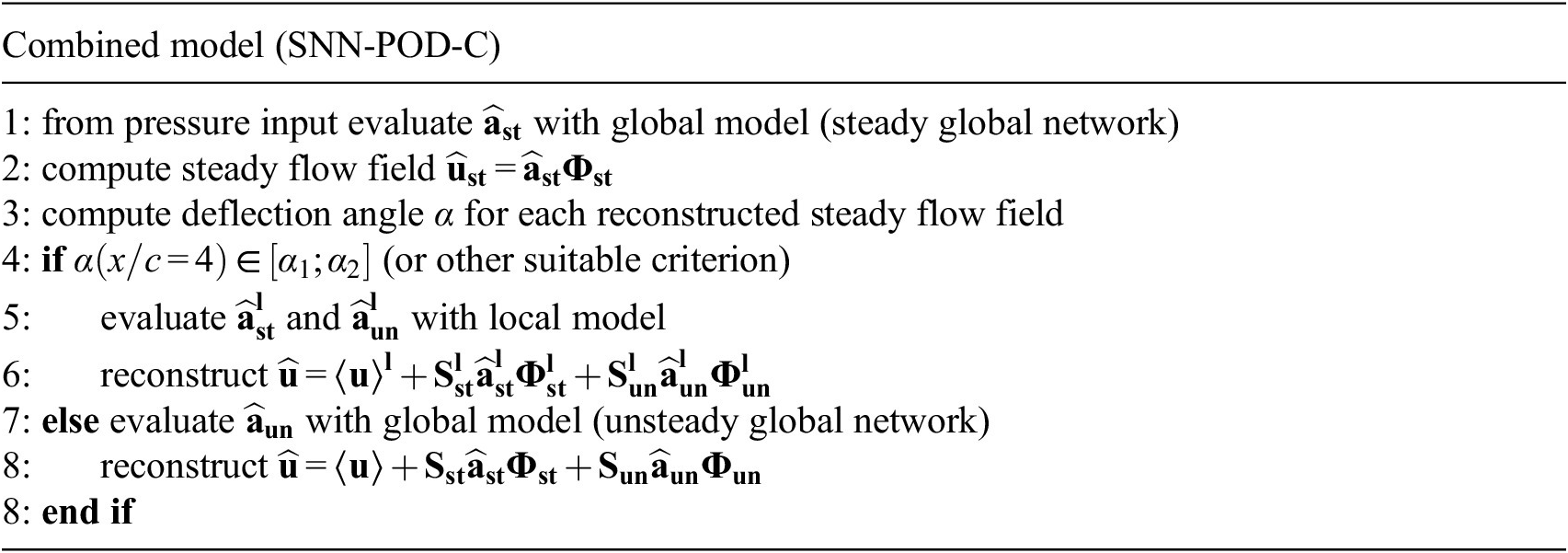
Figure 17 compares the SNN-POD and SNN-POD-C reconstructions with the ground truth at the challenging angle of AoA $ =14{}^{\circ} $
, corresponding to the onset of separation. Comparing the two left columns on each row shows that the instantaneous features of the wake are more accurately captured by the combined model. The mean characteristics of the wake (width and deflection angle), shown in the middle column, are equally well recovered by both models. Comparison of the spectrograms (two right-most columns) confirms that the SNN-POD-C model provides a more accurate estimate of the fluctuation level, which is underestimated by the SNN-POD model.
$ =14{}^{\circ} $
, corresponding to the onset of separation. Comparing the two left columns on each row shows that the instantaneous features of the wake are more accurately captured by the combined model. The mean characteristics of the wake (width and deflection angle), shown in the middle column, are equally well recovered by both models. Comparison of the spectrograms (two right-most columns) confirms that the SNN-POD-C model provides a more accurate estimate of the fluctuation level, which is underestimated by the SNN-POD model.
Side-by-side comparison of streamwise velocity $ u\left(\mathbf{x},{t}_s\right) $
contours at snapshot
$ u\left(\mathbf{x},{t}_s\right) $
contours at snapshot $ {t}_s=150 $
s of the ground truth obtained from URANS (first plot from left to right) and its SNN-POD/SNN-POD-C estimation (second plot). The wake widths and wake deflection angles comparison between the ground truth and the estimation are plotted on the third subfigure. The fourth and fifth plots correspond to the spectrograms of the pre-multiplied velocity spectra
$ {t}_s=150 $
s of the ground truth obtained from URANS (first plot from left to right) and its SNN-POD/SNN-POD-C estimation (second plot). The wake widths and wake deflection angles comparison between the ground truth and the estimation are plotted on the third subfigure. The fourth and fifth plots correspond to the spectrograms of the pre-multiplied velocity spectra $ {fS}_u $
of the ground truth (G.T., left) and estimation (SNN-POD/SNN-POD-C, right) at the
$ {fS}_u $
of the ground truth (G.T., left) and estimation (SNN-POD/SNN-POD-C, right) at the $ x/c=2 $
section. The same logarithmic colormap is applied for both spectrograms.
$ x/c=2 $
section. The same logarithmic colormap is applied for both spectrograms.

Figure 18 presents the three types of reconstruction errors for the standard SNN-POD (shaded areas) and the combined SNN-POD-C models (denoted by red hatched bars) for the range $ \left[14{}^{\circ},16{}^{\circ}\right] $
. All three errors are reduced by a factor of 2 for the angles
$ \left[14{}^{\circ},16{}^{\circ}\right] $
. All three errors are reduced by a factor of 2 for the angles $ 14{}^{\circ},15{}^{\circ},16{}^{\circ} $
, which are seen during training. Interestingly, no reduction is observed for the interpolated angle of
$ 14{}^{\circ},15{}^{\circ},16{}^{\circ} $
, which are seen during training. Interestingly, no reduction is observed for the interpolated angle of $ 15.5{}^{\circ} $
, which shows that the gain associated with specific training does not necessarily lead to better generalization properties.
$ 15.5{}^{\circ} $
, which shows that the gain associated with specific training does not necessarily lead to better generalization properties.
Mean error $ {E}_{test} $
, fluctuating error
$ {E}_{test} $
, fluctuating error $ {\varepsilon}_{test} $
and projected fluctuating error
$ {\varepsilon}_{test} $
and projected fluctuating error $ {\varepsilon}_{test}^{\boldsymbol{\Phi}} $
for transitional AoA without (colored bars) and with (red hatched bars) the use of a local model. The interpolated AoA
$ {\varepsilon}_{test}^{\boldsymbol{\Phi}} $
for transitional AoA without (colored bars) and with (red hatched bars) the use of a local model. The interpolated AoA $ =15.5{}^{\circ} $
is highlighted in green.
$ =15.5{}^{\circ} $
is highlighted in green.

The main outcome of this coupling framework is that the global model demonstrates good performance in reconstructing instantaneous fields for fully attached and separated regimes, while its training over a wide AoA coverage enables interpolation to unseen configurations. Moreover, thanks to the mode-splitting, the global model can infer the AoA regime, allowing it to be coupled with local models that achieve higher accuracy on the transitional AoA regime.
5. Conclusion
This work describes an efficient data-driven methodology for the one-shot reconstruction of instantaneous velocity fields around a thick 2D airfoil from sparse wall-pressure measurements. The dataset is generated from 2D high-Reynolds-number URANS simulations over a range of angles of attack between 10° and 20°, spanning a variety of flow regimes ranging from attached flow to full separation. Proper Orthogonal Decomposition provides a low-dimensional representation of the velocity field that can be split into steady modes, the amplitudes of which depend mostly on the angle of attack, and a remainder of unsteady modes. The model is constituted by two shallow neural networks that independently predict the unsteady and steady parts of the POD amplitudes from limited surface pressure measurements. A sensor placement strategy based on a maximization variance criterion was found to achieve better accuracy than randomized placements when the number of sensors is kept low. The model is trained on a coarse discretization of the angle of attack range ( $ 1-2{}^{\circ} $
) in order to test its generalization abilities. The maximum reconstruction error (MSE) was found to be 2.9% for sampled angles and 6.6% for interpolated angles. In all cases, the time-averaged flow features at a given angle of attack were well recovered from a single-time set of instantaneous pressure measurements. Reconstruction of the time-dependent features could be improved by combining the model trained over the full range of angles of attack with one trained over a more local range. It is emphasized that this proposed strategy merely aims to highlight one of the multiple possibilities offered by the SNN-POD framework.
$ 1-2{}^{\circ} $
) in order to test its generalization abilities. The maximum reconstruction error (MSE) was found to be 2.9% for sampled angles and 6.6% for interpolated angles. In all cases, the time-averaged flow features at a given angle of attack were well recovered from a single-time set of instantaneous pressure measurements. Reconstruction of the time-dependent features could be improved by combining the model trained over the full range of angles of attack with one trained over a more local range. It is emphasized that this proposed strategy merely aims to highlight one of the multiple possibilities offered by the SNN-POD framework.
Several perspectives for extending the study can be identified. First, in the present manuscript, only variations in AoA were considered to define different flow configurations; however, it would be relevant to investigate the performance of SNN-POD under changes in other parameters, such as turbulence intensity or Reynolds number. Second, the current framework is limited to training on 2D URANS simulations, which cannot capture three-dimensional effects, which are particularly important in near flow separation conditions for thick airfoils. A natural extension is thus the application of SNN-POD to higher-fidelity 3D datasets for the reconstruction of fully unsteady 3D flow fields, ultimately making it a valuable tool for experimentalists.
Finally, the reconstruction methodology has so far been assessed only on static simulations with constant AoA, thereby neglecting the additional nonlinearities and hysteresis effects characteristic of dynamic stall. Extending the model to dynamic AoA variations would constitute thee next step, enabling the evaluation of the model under more complex and unsteady operating conditions. To this end, more sophisticated approaches may be explored, such as those incorporating temporal history to capture coherent turbulent structures within the model.
Data availability statement
Code containing the presented models will be available upon publication at https://doi.org/10.5281/zenodo.17400099 (Bucquet et al., Reference Bucquet, Podvin, Braud and Guilmineau2025).
Acknowledgements
This work was granted access to the HPC resources of IDRIS under the allocation 2025-AD012A16542 made by GENCI.
Author contribution
Conceptualization: Q.B., B.P., C.B., and E.G.; Methodology: Q.B. and B.P.; Data curation: Q.B., C.B., and E.G.; Data visualization: Q.B.; Writing - original draft: Q.B.; Writing - review & editing: Q.B., B.P., C.B., and E.G. All authors approved the final submitted draft.
Funding statement
This research was performed within the French-Swiss project MISTERY funded by the French National Research Agency (ANR PRCI grant no. 266157) and the Swiss National Science Foundation (grant no. 200021L 21271). The authors are thankful to the anonymous reviewers for their helpful suggestions.
Competing interests
The authors declare no competing interests exist.


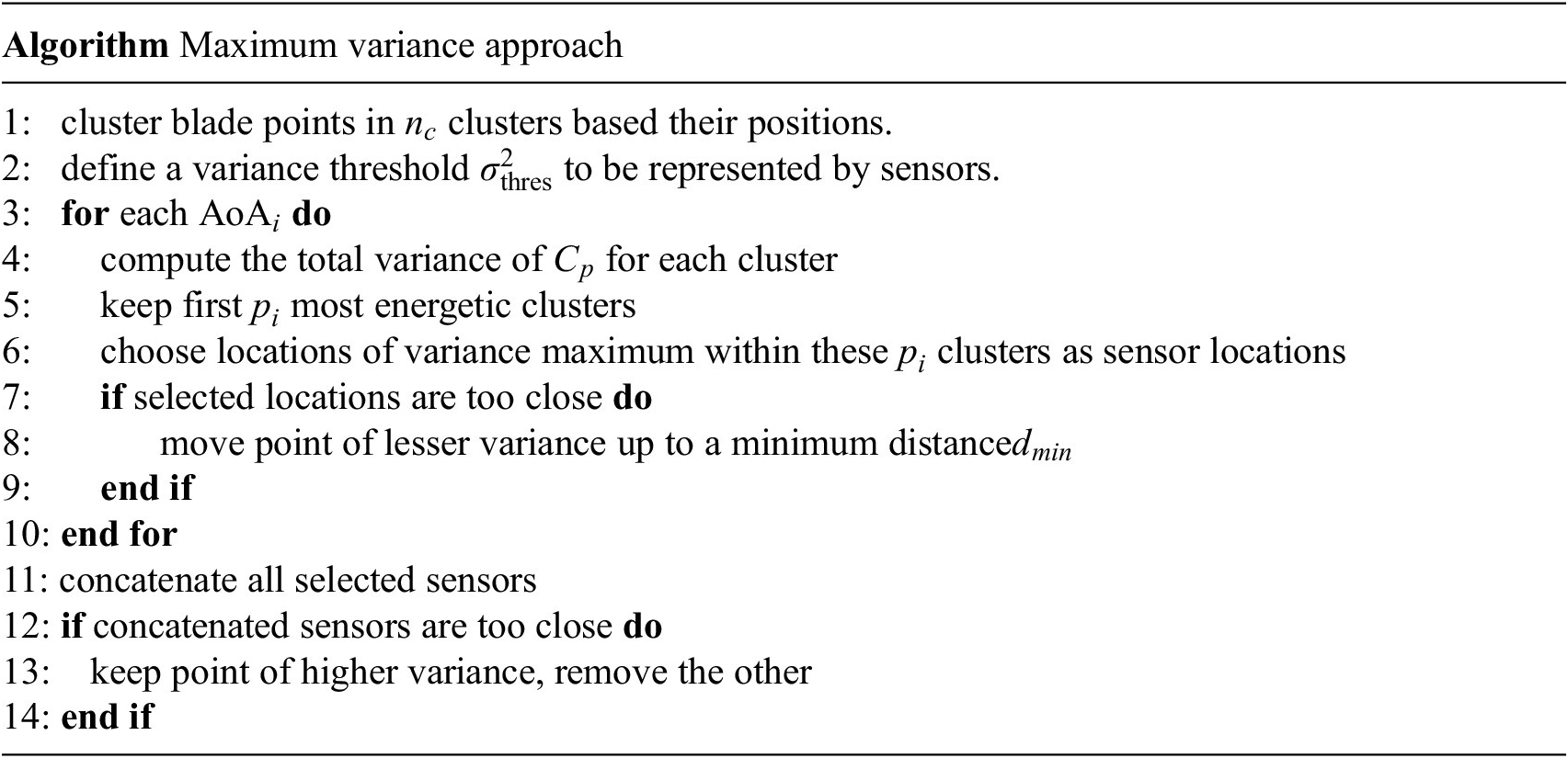




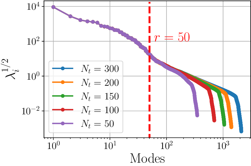


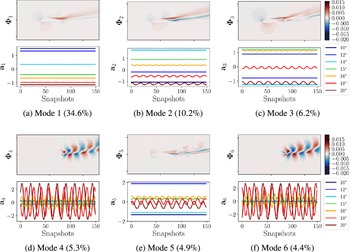





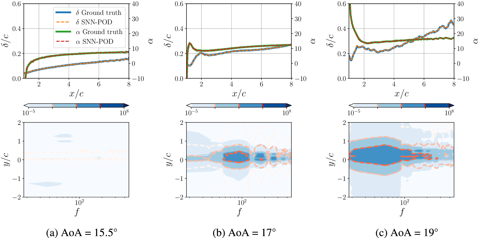


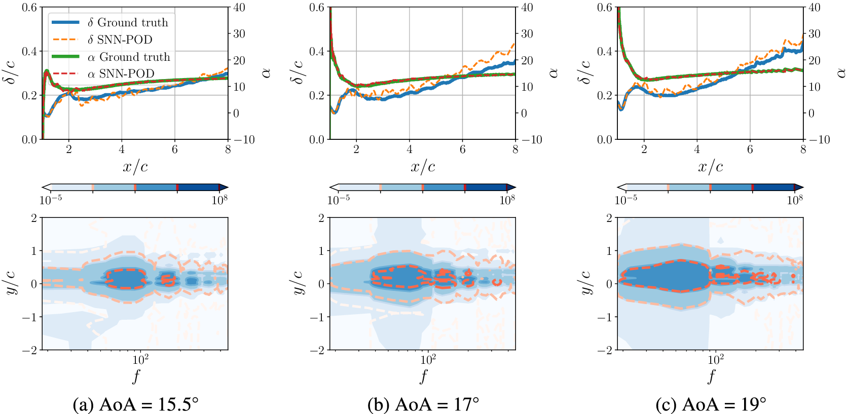


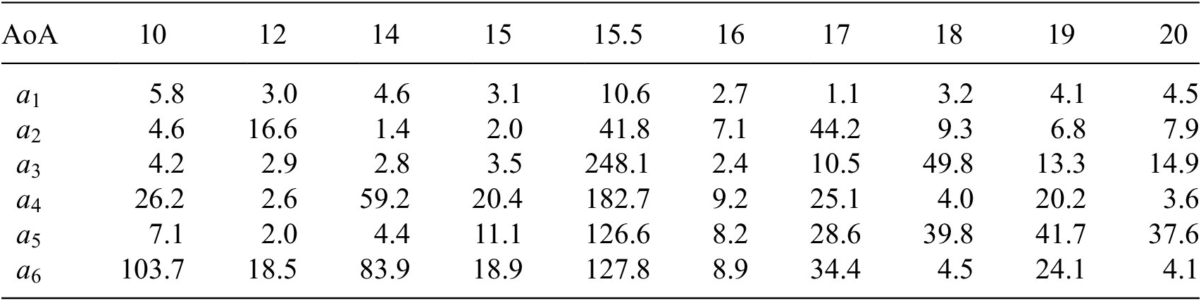





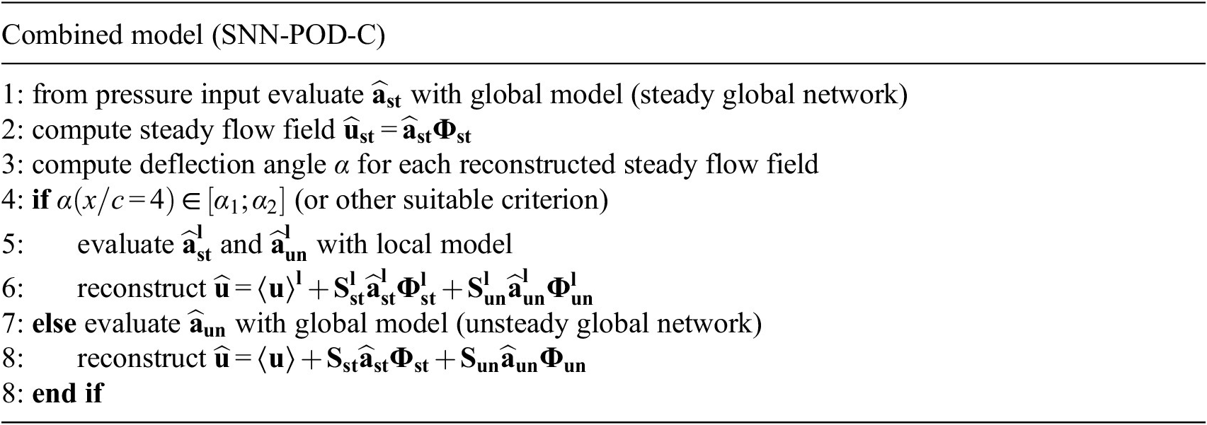


 Open access


Comments
No Comments have been published for this article.