

1. Context and main results
The motivation for this work is the problem of modelling surface runoff. Surface runoff depends on rainfall, infiltration into the soil, and surface topography, all of which vary spatially and temporally. In particular, spatial variation of infiltration and topographical variability make it difficult to fit differential fluid flow models (based on the Navier–Stokes equations) at coarse scales, because parameters lose their physical meaning [Reference Grayson, Moore and McMahon6], while fitting them at fine scales requires high-resolution data and is numerically prohibitively slow.
A practical alternative to measuring the infiltration and topography of a hillslope at high resolution is to summarise small-scale variation statistically, which leads naturally to stochastic runoff models. Suppose that we divide our hillslope into cells. We can model spatial variation of the soil infiltration by supposing that for each cell it is sampled independently from some infiltration distribution. It is known that this variation is enough for a hillslope to produce surface runoff even when the rainfall is less than the average infiltration [Reference Jones, Lane and Sheridan9, Reference Jones, Sheridan and Lane10]. In this work we consider in addition the effect of variation in the micro-topography from one cell to the next.
When surface runoff forms on a hillslope, we see small trickles combining to form larger rivulets, which are proportionally less susceptible to soil infiltration. We call this mechanism coalescence, and we want to show how it affects surface runoff. We suppose that micro-topography will affect the direction of runoff from a cell. Water necessarily flows downhill, but local variation in the topography can mean that instead of taking the most direct route down a slope, a rivulet is diverted to the left or right. We can model this by adding randomness to the direction in which runoff flows out of a cell, where the degree of randomness reflects the roughness of the hillslope.
1.1. An illustrative simulation
We can explore the effect of coalescence with a simple simulation.
Divide a hillslope into a rectangular $m \times n$
grid of cells, so that cells (1,j) are at the top of the slope and cells (m,j) are at the bottom. We suppose that if there is any runoff from cell (i,j), then it can run to cell
$m \times n$
grid of cells, so that cells (1,j) are at the top of the slope and cells (m,j) are at the bottom. We suppose that if there is any runoff from cell (i,j), then it can run to cell $ (i+1,j-1) $
,
$ (i+1,j-1) $
, $ (i+1,j) $
, or
$ (i+1,j) $
, or $ (i+1,j+1) $
with probabilities
$ (i+1,j+1) $
with probabilities ${\delta}$
,
${\delta}$
, $1-2{\delta}$
, and
$1-2{\delta}$
, and ${\delta}$
respectively. This direction does not change over time, and we do not allow runoff to exit via the sides of the grid.
${\delta}$
respectively. This direction does not change over time, and we do not allow runoff to exit via the sides of the grid.
Next, suppose that the rainfall has a constant rate $\rho$
, and that the infiltration rate in cell (i,j) has an exponential distribution with mean 1, independent of other cells. We suppose that the system is in temporal equilibrium, so that at each cell the rates of rainfall, infiltration, runon from above, and runoff do not vary in time. Let
$\rho$
, and that the infiltration rate in cell (i,j) has an exponential distribution with mean 1, independent of other cells. We suppose that the system is in temporal equilibrium, so that at each cell the rates of rainfall, infiltration, runon from above, and runoff do not vary in time. Let $J_{(i,j)}$
be the infiltration rate for cell (i,j) and
$J_{(i,j)}$
be the infiltration rate for cell (i,j) and $W_{(i,j)}$
be the runoff rate from cell (i,j); then we have
$W_{(i,j)}$
be the runoff rate from cell (i,j); then we have
 \begin{equation}\label{eqn1}
W_{(i,j)} = \bigg( \rho - J_{(i,j)} + \sum_{k\,:\,(i-1,k) \to (i,j)} W_{(i-1,k)} \bigg) \vee 0,
\end{equation}
\begin{equation}\label{eqn1}
W_{(i,j)} = \bigg( \rho - J_{(i,j)} + \sum_{k\,:\,(i-1,k) \to (i,j)} W_{(i-1,k)} \bigg) \vee 0,
\end{equation}
where we write $ (i-1,k) \to (i,j) $
if runoff from
$ (i-1,k) \to (i,j) $
if runoff from $ (i-1,k) $
runs on to cell (i,j) (in which case
$ (i-1,k) $
runs on to cell (i,j) (in which case $k \in \{\:j-1,j,j+1\}$
).
$k \in \{\:j-1,j,j+1\}$
).
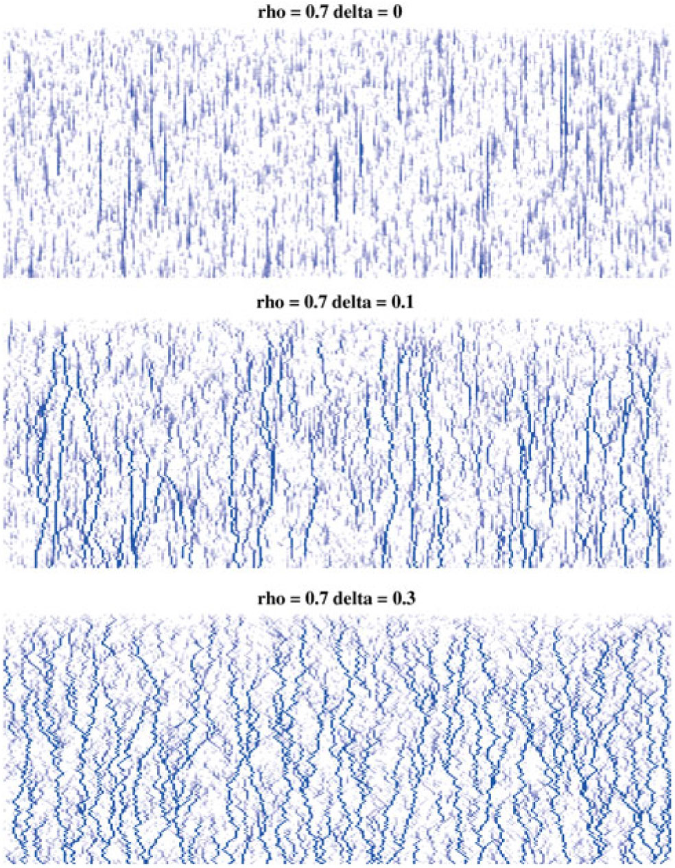
In Figure 1 we give three realisations of this process, for $m=150$
,
$m=150$
, $n=300$
,
$n=300$
, $\rho = 0.7$
, and
$\rho = 0.7$
, and ${\delta} \in \{0, 0.1, 0.3\}$
. We see that for
${\delta} \in \{0, 0.1, 0.3\}$
. We see that for ${\delta}=0$
any runoff that is formed is eventually reabsorbed back into the slope, but for
${\delta}=0$
any runoff that is formed is eventually reabsorbed back into the slope, but for ${\delta}=0.3$
runoff makes its way down the whole slope, even though the average infiltration rate exceeds the rainfall rate. This pattern is consistent for different values of
${\delta}=0.3$
runoff makes its way down the whole slope, even though the average infiltration rate exceeds the rainfall rate. This pattern is consistent for different values of $\rho$
: as
$\rho$
: as ${\delta}$
increases there is increasing runoff; moreover, for any
${\delta}$
increases there is increasing runoff; moreover, for any $\rho$
there is a threshold value of
$\rho$
there is a threshold value of ${\delta}$
after which we start to see runoff making its way down the whole hillslope from top to bottom. In what follows we will develop an abstract model for runoff for which we can establish this phase change precisely.
${\delta}$
after which we start to see runoff making its way down the whole hillslope from top to bottom. In what follows we will develop an abstract model for runoff for which we can establish this phase change precisely.
Simulation output illustrating the effect of coalescing streams. In each case water flows from top to bottom; the darker the pixel the greater the flow. Each cell has rainfall rate $\rho$
, a random infiltration rate with mean 1, a chance
$\rho$
, a random infiltration rate with mean 1, a chance ${\delta}$
that runoff is directed down and to the left, and a chance
${\delta}$
that runoff is directed down and to the left, and a chance ${\delta}$
that it is directed down and to the right. For
${\delta}$
that it is directed down and to the right. For ${\delta}=0$
any runoff that is formed is eventually reabsorbed back into the slope, but for
${\delta}=0$
any runoff that is formed is eventually reabsorbed back into the slope, but for ${\delta}=0.3$
runoff makes its way down the whole slope, even though the average infiltration rate exceeds the rainfall rate. Note that the three plots have been scaled so that the maximum runoff is the same shade; the maximum runoff actually increases with
${\delta}=0.3$
runoff makes its way down the whole slope, even though the average infiltration rate exceeds the rainfall rate. Note that the three plots have been scaled so that the maximum runoff is the same shade; the maximum runoff actually increases with ${\delta}$
. The code can be found at http://researchers.ms.unimelb.edu.au/
${\delta}$
. The code can be found at http://researchers.ms.unimelb.edu.au/ $\sim$
apro@unimelb/spuRs/index.html.
$\sim$
apro@unimelb/spuRs/index.html.
1.2. Drainage trees
Suppose that we have a hillslope divided into cells, and that the runoff from any given cell will flow into a unique cell below. For example, using a square lattice we could allow runoff into any one of the three cells below with a common edge or vertex, or using a diamond lattice we might choose to allow runoff into either of the two cells below with a common edge. Examples of the runoff paths that can be generated in these two cases are given in Figure 2. Selecting a single cell at the bottom of the hillslope and then considering all the cells that could potentially drain into it we get a rooted tree, which we call a drainage tree, where the nodes correspond to cells and edges indicate where runoff flows from one cell to the next (runoff is always towards the root).
Two realisations of paths of potential runoff, for a square lattice (left) and a diamond lattice (right). In either case, if we take a single cell at the bottom and consider all the cells that could drain into it we get a tree.
In what follows we will consider runoff on a single drainage tree. Given a rooted tree, let $X_i$
be the difference between rainfall and infiltration in cell i, and denote by
$X_i$
be the difference between rainfall and infiltration in cell i, and denote by $\{\:j\,:\,j\to i\}$
those cells that send runoff directly into node i. The runoff from cell/node i is then
$\{\:j\,:\,j\to i\}$
those cells that send runoff directly into node i. The runoff from cell/node i is then
 \begin{equation}
W_i =\bigg( X_i + \sum_{j\,:\,j\to i} W_j \bigg) \vee 0.
\end{equation}
\begin{equation}
W_i =\bigg( X_i + \sum_{j\,:\,j\to i} W_j \bigg) \vee 0.
\end{equation}
We can view the $X_i$
as either rates or, if we integrate over discrete time periods, volumes. In either case we are assuming that the system is temporally homogeneous and in equilibrium.
$X_i$
as either rates or, if we integrate over discrete time periods, volumes. In either case we are assuming that the system is temporally homogeneous and in equilibrium.
Our object of interest is $W_0$
, where 0 is the root. If the tree is finite then
$W_0$
, where 0 is the root. If the tree is finite then $W_0$
is clearly well defined: we have
$W_0$
is clearly well defined: we have $W_j = X_j \vee 0$
for all leaves j, so we can use (1) to recursively calculate
$W_j = X_j \vee 0$
for all leaves j, so we can use (1) to recursively calculate $W_i$
for all the other nodes. For infinite trees we define
$W_i$
for all the other nodes. For infinite trees we define $W_0 = \lim_{n\to\infty} W_0^{(n)}$
, where
$W_0 = \lim_{n\to\infty} W_0^{(n)}$
, where $W_0^{(n)}$
is the root-runoff from the tree truncated at generation/height n. The
$W_0^{(n)}$
is the root-runoff from the tree truncated at generation/height n. The $W_0^{(n)}$
are clearly non-decreasing so
$W_0^{(n)}$
are clearly non-decreasing so $W_0$
exists, though may be improper.
$W_0$
exists, though may be improper.
It is interesting to note that if instead of working our way down from the leaves we consider working our way up from the root, then we get
 \begin{equation}
W_0 =
%\max_{\scriptsize\begin{tabular}{c}rooted\\ subtrees \textit{T}\end{tabular}}
\max_{T \in \{{\rm rooted\ subtrees} \}}
\sum_{i \in T} X_i ,
\end{equation}
\begin{equation}
W_0 =
%\max_{\scriptsize\begin{tabular}{c}rooted\\ subtrees \textit{T}\end{tabular}}
\max_{T \in \{{\rm rooted\ subtrees} \}}
\sum_{i \in T} X_i ,
\end{equation}
where a rooted subtree is any subtree including the root 0, or the empty subtree (in which case we take the sum to be 0).
1.3. Drainage trees from the diamond lattice
In hydrology the use of the diamond lattice to generate random drainage patterns can be traced back to Scheidegger [Reference Scheidegger14]. Note, however, that in the hydrological literature drainage trees are used to describe river networks, rather than the small-scale patterns of ephemeral surface runoff that we are interested in.
Take as our hillslope a half-plane extending upwards ad infinitum, and divide it into cells using a diamond lattice. Furthermore, suppose that from each cell runoff goes left with probability ${\beta} \in (0, 1) $
and right with probability
${\beta} \in (0, 1) $
and right with probability ${\,\overline{\!\beta}} = 1 - {\beta}$
, independently of all other cells. Consider the drainage tree attached to a single cell at the bottom of the slope. If we think of the tree as growing from its root, then for any node the number of offspring has the distribution
${\,\overline{\!\beta}} = 1 - {\beta}$
, independently of all other cells. Consider the drainage tree attached to a single cell at the bottom of the slope. If we think of the tree as growing from its root, then for any node the number of offspring has the distribution
 \begin{equation}
\begin{array}{r|ccc}
z & 0 & 1 & 2 \\
\hline
{\mathrm P}(Z=z) & {\beta}{\,\overline{\!\beta}} & {\beta}^2 + {\,\overline{\!\beta}}^2 & {\beta}{\,\overline{\!\beta}} %.
\end{array}
\end{equation}
\begin{equation}
\begin{array}{r|ccc}
z & 0 & 1 & 2 \\
\hline
{\mathrm P}(Z=z) & {\beta}{\,\overline{\!\beta}} & {\beta}^2 + {\,\overline{\!\beta}}^2 & {\beta}{\,\overline{\!\beta}} %.
\end{array}
\end{equation}
If ${\beta} = 0$
or 1 then our tree degenerates to one dimension, but is infinite in size. This case is considered in [9, 10], and from here on we will assume that
${\beta} = 0$
or 1 then our tree degenerates to one dimension, but is infinite in size. This case is considered in [9, 10], and from here on we will assume that ${\beta} \in (0, 1/2]$
, unless stated otherwise. We can interpret
${\beta} \in (0, 1/2]$
, unless stated otherwise. We can interpret ${\beta}$
in terms of surface roughness:
${\beta}$
in terms of surface roughness: ${\beta}=1/2$
gives the roughest surface, with decreasing values corresponding to smoother surfaces. In terms of our model, we get the greatest degree of coalescence when
${\beta}=1/2$
gives the roughest surface, with decreasing values corresponding to smoother surfaces. In terms of our model, we get the greatest degree of coalescence when ${\beta}=1/2$
, and the least (none) when
${\beta}=1/2$
, and the least (none) when ${\beta} = 0$
. The cases
${\beta} = 0$
. The cases ${\beta}$
and
${\beta}$
and $1-{\beta}$
are equivalent by symmetry.
$1-{\beta}$
are equivalent by symmetry.
Clearly, unlike a Bienaymé–Galton–Watson (BGW) process, for a lattice-derived tree the family sizes in any given generation are dependent. Let $Z_n$
be the number of nodes in generation n (where the root is generation 0); then we have that
$Z_n$
be the number of nodes in generation n (where the root is generation 0); then we have that $Z_{n+1} = Z_n + D_n$
, where
$Z_{n+1} = Z_n + D_n$
, where $D_n$
is independent of
$D_n$
is independent of $Z_n$
and has the distribution
$Z_n$
and has the distribution
 \begin{equation}
\begin{array}{r|ccc}
k & -1 & 0 & 1 \\
\hline
{\mathrm P}(D_n=k) & {\beta}{\,\overline{\!\beta}} & {\beta}^2 + {\,\overline{\!\beta}}^2 & {\beta}{\,\overline{\!\beta}} %.
\end{array}
\end{equation}
\begin{equation}
\begin{array}{r|ccc}
k & -1 & 0 & 1 \\
\hline
{\mathrm P}(D_n=k) & {\beta}{\,\overline{\!\beta}} & {\beta}^2 + {\,\overline{\!\beta}}^2 & {\beta}{\,\overline{\!\beta}} %.
\end{array}
\end{equation}
That is, the tree diameter is given by a random walk with zero drift, from which it follows immediately that the tree is almost surely (a.s.) finite, but that its expected height is infinite.
To see where the distribution of $D_n$
comes from, consider Figure 3. Here we have labelled the nodes of the lattice relative to the root of the tree. In generation n the tree consists of all nodes from
$D_n$
comes from, consider Figure 3. Here we have labelled the nodes of the lattice relative to the root of the tree. In generation n the tree consists of all nodes from $L_n$
to
$L_n$
to $R_n$
say, where
$R_n$
say, where $Z_n = R_n - L_n$
. We see that
$Z_n = R_n - L_n$
. We see that $L_{n+1} = L_n$
with probability
$L_{n+1} = L_n$
with probability ${\,\overline{\!\beta}}$
and
${\,\overline{\!\beta}}$
and $L_n+1$
with probability
$L_n+1$
with probability ${\beta}$
, depending on the direction of the runoff from the above-left cell. Similarly,
${\beta}$
, depending on the direction of the runoff from the above-left cell. Similarly, $R_{n+1} = R_n$
with probability
$R_{n+1} = R_n$
with probability ${\,\overline{\!\beta}}$
and
${\,\overline{\!\beta}}$
and $R_n+1$
with probability
$R_n+1$
with probability ${\beta}$
, independently of
${\beta}$
, independently of $L_{n+1}$
. We then have
$L_{n+1}$
. We then have $D_{n+1} = R_{n+1} - R_n - L_{n+1} + L_n$
, which has the distribution (4).
$D_{n+1} = R_{n+1} - R_n - L_{n+1} + L_n$
, which has the distribution (4).
A tree on the diamond lattice with nodes in each generation numbered relative to the leftmost possible position. At each generation the tree contains all nodes between some left limit $L_n$
and right limit
$L_n$
and right limit $R_n$
. From one generation to the next, the number of nodes can increase or decrease by at most 1.
$R_n$
. From one generation to the next, the number of nodes can increase or decrease by at most 1.
In what follows we will approximate the diamond lattice tree with a critical BGW tree by the simple expediency of dropping the dependence between offspring numbers in each generation. That is, we use the offspring distribution (3).
1.4. Runoff on a critical BGW tree
Suppose that we are given a critical BGW tree with offspring distribution (3) for ${\beta} \in (0, 1/2]$
. We associate independent and identically distributed (i.i.d.) random variables
${\beta} \in (0, 1/2]$
. We associate independent and identically distributed (i.i.d.) random variables $X_i$
with each node, and are interested in the
$X_i$
with each node, and are interested in the $W_i$
as defined by (1).
$W_i$
as defined by (1).
Write X and W for $X_0$
and
$X_0$
and $W_0$
, the point contribution and net runoff at the root, and let
$W_0$
, the point contribution and net runoff at the root, and let $W_{\rm L}$
be the runoff from the cell above left and
$W_{\rm L}$
be the runoff from the cell above left and $W_{\rm R}$
the runoff from the cell above right. From the self-similar structure of the BGW tree we have that W,
$W_{\rm R}$
the runoff from the cell above right. From the self-similar structure of the BGW tree we have that W, $W_{\rm L}$
, and
$W_{\rm L}$
, and $W_{\rm R}$
are identically distributed, and
$W_{\rm R}$
are identically distributed, and $W_{\rm L}$
and
$W_{\rm L}$
and $W_{\rm R}$
are independent.
$W_{\rm R}$
are independent.
Let $I_{\rm L}$
indicate if the cell above left drains into the root cell, and similarly for
$I_{\rm L}$
indicate if the cell above left drains into the root cell, and similarly for $I_{\rm R}$
; then
$I_{\rm R}$
; then ${\mathrm E}(I_{\rm L}) = {\,\overline{\!\beta}}$
,
${\mathrm E}(I_{\rm L}) = {\,\overline{\!\beta}}$
, ${\mathrm E}( I_{\rm R}) = {\beta}$
, and
${\mathrm E}( I_{\rm R}) = {\beta}$
, and
 \begin{equation}
W \eqdist (W_{\rm L} I_{\rm L} + W_{\rm R} I_{\rm R} + X) \vee 0.
\end{equation}
\begin{equation}
W \eqdist (W_{\rm L} I_{\rm L} + W_{\rm R} I_{\rm R} + X) \vee 0.
\end{equation}
This equation is the focus of the remainder of the paper. We know that an a.s. finite solution W exists, because we can construct one. By iterating the right-hand side of (5) we get a set of equations of the form (1), where the underlying tree is a realisation of a critical BGW tree with offspring distribution given by (3). This critical BGW tree is a.s. finite, so the solutions we construct using (1) are a.s. finite. We will only consider a.s. finite solutions to (5). In general it is not clear whether there is more than one solution; however, in the cases we consider we obtain unique expressions for the probability-generating function (pgf) of W, assuming that W is a.s. finite (see Propositions 4 and 6). That is, in the cases we consider we have a unique finite solution.
We summarise our main results here, and defer the proofs to the next two sections. Section 4 then discusses some generalisations. In order to obtain exact results we will suppose that X has the following distribution, for some ${\alpha} \in (0, 1) $
:
${\alpha} \in (0, 1) $
:
 \begin{equation}\label{X.eqn}
\begin{array}{r|cc}
x & 1 & -1 \\
\hline
{\mathrm P}(X=x) & {\alpha} & {\overline{\alpha}} = 1-{\alpha}
\end{array}
\end{equation}
\begin{equation}\label{X.eqn}
\begin{array}{r|cc}
x & 1 & -1 \\
\hline
{\mathrm P}(X=x) & {\alpha} & {\overline{\alpha}} = 1-{\alpha}
\end{array}
\end{equation}
If ${\alpha} = 0$
then
${\alpha} = 0$
then $W = 0$
, while if
$W = 0$
, while if ${\alpha} = 1$
then W is just the size of the tree.
${\alpha} = 1$
then W is just the size of the tree.
Proposition 1. Put
 \begin{equation}\label{a_c.eqn}
{\alpha}_{\rm c}({\beta}) = (1/2) ( 1 + {\beta}{\,\overline{\!\beta}} - \sqrt{{\beta}{\,\overline{\!\beta}} (2 + {\beta}{\,\overline{\!\beta}})} ).
\end{equation}
\begin{equation}\label{a_c.eqn}
{\alpha}_{\rm c}({\beta}) = (1/2) ( 1 + {\beta}{\,\overline{\!\beta}} - \sqrt{{\beta}{\,\overline{\!\beta}} (2 + {\beta}{\,\overline{\!\beta}})} ).
\end{equation}
Then, for ${\alpha} \leq {\alpha}_{\rm c}({\beta}) $
,
${\alpha} \leq {\alpha}_{\rm c}({\beta}) $
,
 \begin{equation}\label{Ex_W.eqn}
{\mathrm E}( W) = \frac 1{2{\beta}(1-{\beta})} ( 1 - 2{\alpha} - \sqrt{1 - 4{\alpha}(1 - {\alpha} + {\beta}(1-{\beta}))} ),
\end{equation}
\begin{equation}\label{Ex_W.eqn}
{\mathrm E}( W) = \frac 1{2{\beta}(1-{\beta})} ( 1 - 2{\alpha} - \sqrt{1 - 4{\alpha}(1 - {\alpha} + {\beta}(1-{\beta}))} ),
\end{equation}
while for ${\alpha} > {\alpha}_{\rm c}({\beta}) $
,
${\alpha} > {\alpha}_{\rm c}({\beta}) $
, ${\mathrm E}( W) = \infty$
.
${\mathrm E}( W) = \infty$
.
Figure 4 gives a plot of ${\alpha}_{\rm c}$
. Figure 5 gives plots of
${\alpha}_{\rm c}$
. Figure 5 gives plots of ${\mathrm E}( W) $
against
${\mathrm E}( W) $
against ${\alpha}$
for various
${\alpha}$
for various ${\beta}$
.
${\beta}$
.
The function
 ${\alpha}_{\rm c}({\beta}) =
(1/2) ( 1 + {\beta}{\,\overline{\!\beta}} - \sqrt{{\beta}{\,\overline{\!\beta}} (2 + {\beta}{\,\overline{\!\beta}})}) $
.
${\alpha}_{\rm c}({\beta}) =
(1/2) ( 1 + {\beta}{\,\overline{\!\beta}} - \sqrt{{\beta}{\,\overline{\!\beta}} (2 + {\beta}{\,\overline{\!\beta}})}) $
.
Expected runoff for various values of ${\alpha}$
and
${\alpha}$
and ${\beta}$
. For
${\beta}$
. For ${\alpha}$
larger than the given ranges, the expected mean is
${\alpha}$
larger than the given ranges, the expected mean is $\infty$
.
$\infty$
.
Note that for all ${\beta} > 0$
we have
${\beta} > 0$
we have ${\alpha}_{\rm c}({\beta}) \lt 1/2$
, so that
${\alpha}_{\rm c}({\beta}) \lt 1/2$
, so that ${\mathrm E}( X) \lt 0$
. That is, the critical point at which the expected runoff becomes infinite happens when the rainfall is less than the expected infiltration. Moreover, as the degree of coalescence increases, i.e. as
${\mathrm E}( X) \lt 0$
. That is, the critical point at which the expected runoff becomes infinite happens when the rainfall is less than the expected infiltration. Moreover, as the degree of coalescence increases, i.e. as ${\beta} \uparrow 1/2$
, less rainfall is required to reach the critical point. We say that the runoff is subcritical/critical/supercritical as
${\beta} \uparrow 1/2$
, less rainfall is required to reach the critical point. We say that the runoff is subcritical/critical/supercritical as ${\alpha}$
is less than / equal to / greater than
${\alpha}$
is less than / equal to / greater than ${\alpha}_{\rm c}$
.
${\alpha}_{\rm c}$
.
We can say more about the size of W, in terms of how heavy its tail is.
Proposition 2. Put
 \begin{equation}\label{h.eqn}
h(t) = \frac {t[1 - {\alpha}(4{\beta}{\,\overline{\!\beta}} + t) - {\alpha}^2(1-2{\beta})^2(1-t^2)]}
{4{\overline{\alpha}}{\beta}^2{\,\overline{\!\beta}}^2(1 - {\alpha}(1-t^2))} ,
\end{equation}
\begin{equation}\label{h.eqn}
h(t) = \frac {t[1 - {\alpha}(4{\beta}{\,\overline{\!\beta}} + t) - {\alpha}^2(1-2{\beta})^2(1-t^2)]}
{4{\overline{\alpha}}{\beta}^2{\,\overline{\!\beta}}^2(1 - {\alpha}(1-t^2))} ,
\end{equation}
and let $t_0$
be the point at which h achieves its maximum in [0, 1]. Then, as
$t_0$
be the point at which h achieves its maximum in [0, 1]. Then, as $x \to \infty$
,
$x \to \infty$
,
 \begin{equation}
{\mathrm P}(W > x) \sim
\left\{\!\!\begin{array}{ll}
\sqrt{ \frac {-h''(1)(1-{\alpha})}{8\pi}} x^{-3/2} & {\alpha} = {\alpha}_{\rm c} , \\
\sqrt{ \frac {(h(t_0) - h(1))(1-{\alpha})}\pi } x^{-1/2} & {\alpha} > {\alpha}_{\rm c} .
\end{array}\right.
\end{equation}
\begin{equation}
{\mathrm P}(W > x) \sim
\left\{\!\!\begin{array}{ll}
\sqrt{ \frac {-h''(1)(1-{\alpha})}{8\pi}} x^{-3/2} & {\alpha} = {\alpha}_{\rm c} , \\
\sqrt{ \frac {(h(t_0) - h(1))(1-{\alpha})}\pi } x^{-1/2} & {\alpha} > {\alpha}_{\rm c} .
\end{array}\right.
\end{equation}
For ${\alpha} < {\alpha}_{\rm c}$
, W has all positive moments finite.
${\alpha} < {\alpha}_{\rm c}$
, W has all positive moments finite.
Let $N_T$
be the total number of nodes in our drainage tree; then it is known that
$N_T$
be the total number of nodes in our drainage tree; then it is known that
 \begin{equation}\label{NT.eqn}
{\mathrm P}(N_T = n) \approx n^{-3/2} \frac 1{2\sqrt{\pi{\beta}{\,\overline{\!\beta}}}\,}.
\end{equation}
\begin{equation}\label{NT.eqn}
{\mathrm P}(N_T = n) \approx n^{-3/2} \frac 1{2\sqrt{\pi{\beta}{\,\overline{\!\beta}}}\,}.
\end{equation}
We give a sketch of the proof in Section 3.1. In particular, even though $N_T$
is almost surely finite, we have
$N_T$
is almost surely finite, we have ${\mathrm E}( N_T) = \infty$
. This suggests that when
${\mathrm E}( N_T) = \infty$
. This suggests that when ${\mathrm E}( W) = \infty$
it is because the runoff at the root is getting contributions from all over the tree, where we say that a node i contributes to the runoff at the root if there is a path
${\mathrm E}( W) = \infty$
it is because the runoff at the root is getting contributions from all over the tree, where we say that a node i contributes to the runoff at the root if there is a path $ (i_1 = i, i_2, \ldots, i_n = 0) $
from i to the root such that
$ (i_1 = i, i_2, \ldots, i_n = 0) $
from i to the root such that $W_{i_k} > 0$
for all k. Our final result for this section says that this is indeed the case. Moreover, we see that when
$W_{i_k} > 0$
for all k. Our final result for this section says that this is indeed the case. Moreover, we see that when ${\mathrm E}( W) < \infty$
only the bottom of the tree is contributing.
${\mathrm E}( W) < \infty$
only the bottom of the tree is contributing.
We can re-express (5) as
 \begin{align}
W &= (W_{\rm L}I_{\rm L} + W_{\rm R}I_{\rm R} + X) \vee 0 \nonumber \\
&= W_{\rm L}I_{\rm L} + W_{\rm R}I_{\rm R} + Y ,
\end{align}
\begin{align}
W &= (W_{\rm L}I_{\rm L} + W_{\rm R}I_{\rm R} + X) \vee 0 \nonumber \\
&= W_{\rm L}I_{\rm L} + W_{\rm R}I_{\rm R} + Y ,
\end{align}
where Y is the net contribution to runoff from our cell. $W_{\rm L}$
,
$W_{\rm L}$
, $W_{\rm R}$
,
$W_{\rm R}$
, $I_{\rm L}$
,
$I_{\rm L}$
, $I_{\rm R}$
, and X are all in-dependent, but the distribution of Y depends on X,
$I_{\rm R}$
, and X are all in-dependent, but the distribution of Y depends on X, $W_{\rm L}$
,
$W_{\rm L}$
, $W_{\rm R}$
,
$W_{\rm R}$
, $I_{\rm L}$
, and
$I_{\rm L}$
, and $I_{\rm R}$
.
$I_{\rm R}$
.
Proposition 3. When ${\alpha} > {\alpha}_{\rm c}$
we have
${\alpha} > {\alpha}_{\rm c}$
we have ${\mathrm E}( Y) > 0$
, and for every
${\mathrm E}( Y) > 0$
, and for every ${\delta} > 0$
there is an
${\delta} > 0$
there is an ${\varepsilon} > 0$
such that
${\varepsilon} > 0$
such that
 \begin{equation}
{\mathrm P}( \mbox{$100(1-{\delta})\%$ of the tree height contributes to root runoff} ) \geq {\varepsilon}.
\end{equation}
\begin{equation}
{\mathrm P}( \mbox{$100(1-{\delta})\%$ of the tree height contributes to root runoff} ) \geq {\varepsilon}.
\end{equation}
When ${\alpha} \leq {\alpha}_{\rm c}$
we have
${\alpha} \leq {\alpha}_{\rm c}$
we have ${\mathrm E}( Y) = 0$
, and the expected tree height contributing to root runoff is finite.
${\mathrm E}( Y) = 0$
, and the expected tree height contributing to root runoff is finite.
We finish the section with a hydrologically inclined qualitative summary of our results.
Summary. When the rainfalls subcritical, only the bottom of the hillslope contributes to runoff, but when the rainfall is supercritical, the whole slope starts contributing, giving a phase change in the amount of runoff produced. The critical point depends on the degree of coalescence induced by the micro-topography of the hillslope.
1.5. Links to other work
The pattern of drainage trees produced by the diamond lattice is a familiar probabilistic object, known as coalescing random walks or the voter model in dimension one; see, for example, the books of Liggett [Reference Liggett12] or Durrett [Reference Durrett3].
As noted above, the offspring numbers in generation n of a drainage tree are dependent. When producing generation $n+1$
from generation n, we can group the nodes into runs with a single offspring above left, and runs with a single offspring above right. When you switch from one type of run to the other you get a node with either two or zero offspring. We can map these runs to runs in a sequence of independent Bernoulli random variables, which have been studied in the context of various non-parametric statistics, most notably in [Reference Wald and Wolfowitz17].
$n+1$
from generation n, we can group the nodes into runs with a single offspring above left, and runs with a single offspring above right. When you switch from one type of run to the other you get a node with either two or zero offspring. We can map these runs to runs in a sequence of independent Bernoulli random variables, which have been studied in the context of various non-parametric statistics, most notably in [Reference Wald and Wolfowitz17].
Huber [Reference Huber7] and Takayasu & Takayasu [Reference Takayasu, Takayasu and Privman15] have considered sums of the form $\sum_{i\in T} X_i$
where T is a drainage tree arising from a diamond lattice, and the
$\sum_{i\in T} X_i$
where T is a drainage tree arising from a diamond lattice, and the $X_i$
are i.i.d. They used the tree to model the aggregation of charged particles.
$X_i$
are i.i.d. They used the tree to model the aggregation of charged particles.
In the case where ${\beta} = 0$
and the drainage tree has dimension one, (1) is the same as the equation for the waiting time in a single-server queue. In the queueing theory literature much use is made of the time-reversed process, which satisfies the same equation as the original. In our case, reversing the process gives (2) instead.
${\beta} = 0$
and the drainage tree has dimension one, (1) is the same as the equation for the waiting time in a single-server queue. In the queueing theory literature much use is made of the time-reversed process, which satisfies the same equation as the original. In our case, reversing the process gives (2) instead.
Equations of type (5) are known as distributional fixed-point equations or recursive distributional equations, and there is some general theory on the existence and uniqueness of solutions to such equations [Reference Aldous and Bandyopadhyay1, Reference Jelenković, Olvera-Cravioto, Alsmeyer and Löwe8]. In the terminology of [Reference Aldous and Bandyopadhyay1], the a.s. finite solution we consider here is endogenous.
When X takes values on $\{-1, 0, 1, \ldots\}$
, Goldschmidt & Pryzykucki [Reference Goldschmidt and Przykucki5] observe that the runoff process is equivalent to a parking process, used to analyse the performance of hash tables. They have a number of nice results for parking on a critical BGW tree with Poisson offsping numbers, on subcritical and supercritical BGW trees, and they conjecture about more general behaviour on critical trees.
$\{-1, 0, 1, \ldots\}$
, Goldschmidt & Pryzykucki [Reference Goldschmidt and Przykucki5] observe that the runoff process is equivalent to a parking process, used to analyse the performance of hash tables. They have a number of nice results for parking on a critical BGW tree with Poisson offsping numbers, on subcritical and supercritical BGW trees, and they conjecture about more general behaviour on critical trees.
2. Proofs: The mean and right tail of W
Since $X \in {\mathbb Z}$
we have
$X \in {\mathbb Z}$
we have $W \in {\mathbb Z}_+$
, and we define
$W \in {\mathbb Z}_+$
, and we define $p_i = {\mathrm P}(W = i) $
. For convenience we also define
$p_i = {\mathrm P}(W = i) $
. For convenience we also define $p_0^{\rm L} = {\mathrm P}(W_{\rm L}I_{\rm L} = 0) = {\beta} + {\,\overline{\!\beta}} p_0$
and
$p_0^{\rm L} = {\mathrm P}(W_{\rm L}I_{\rm L} = 0) = {\beta} + {\,\overline{\!\beta}} p_0$
and $p_0^{\rm R} = {\mathrm P}(W_{\rm R}I_{\rm R} = 0) = {\,\overline{\!\beta}} + {\beta} p_0$
. Let f be the pgf of W,
$p_0^{\rm R} = {\mathrm P}(W_{\rm R}I_{\rm R} = 0) = {\,\overline{\!\beta}} + {\beta} p_0$
. Let f be the pgf of W, $f(t) = {\mathrm E}( t^W) $
; then, from (5) we have
$f(t) = {\mathrm E}( t^W) $
; then, from (5) we have
 \begin{align*}
f(t) \,&=\, {\mathrm E}( t^{I_{\rm L}W_{\rm L} + I_{\rm R}W_{\rm R} + X \vee 0}) \\
&=\, {\mathrm E}( t^{I_{\rm L}W_{\rm L} + I_{\rm R}W_{\rm R} + 1} I_{\{X=1\}}) \\
&\quad +\,{\mathrm E}( I_{\{X=-1\}} I_{\{I_{\rm L}W_{\rm L} = 0\}} I_{\{I_{\rm R}W_{\rm R} = 0\}}) \\
&\quad +\,{\mathrm E}( t^{I_{\rm L}W_{\rm L} - 1} I_{\{X=-1\}} I_{\{I_{\rm L}W_{\rm L} > 0\}} I_{\{I_{\rm R}W_{\rm R} = 0\}}) \\
&\quad +\,{\mathrm E}( t^{I_{\rm R}W_{\rm R} - 1} I_{\{X=-1\}} I_{\{I_{\rm L}W_{\rm L} = 0\}} I_{\{I_{\rm R}W_{\rm R} > 0\}}) \\
&\quad +\,{\mathrm E}( t^{I_{\rm L}W_{\rm L} + I_{\rm R}W_{\rm R} - 1} I_{\{X=-1\}} I_{\{I_{\rm L}W_{\rm L} > 0\}} I_{\{I_{\rm R}W_{\rm R} > 0\}}) \\
&=\, {\alpha} ({\beta} + (1-{\beta})f(t)) (1-{\beta} + {\beta} f(t)) t \\
&\quad +\,(1-{\alpha}) p_0^{\rm L} p_0^{\rm R} \\
&\quad +\,(1-{\alpha}) p_0^{\rm R} (1-{\beta}) (f(t) - p_0) t^{-1} \\
&\quad +\,(1-{\alpha}) p_0^{\rm L} {\beta} (f(t) - p_0) t^{-1} \\
&\quad +\,(1-{\alpha}) {\beta} (1-{\beta}) (f(t) - p_0)^2 t^{-1} \\
&=\, t^{-1} [ (1-{\alpha}) (1 - 2{\beta} + 2 {\beta}^2) p_0 (t - 1) \\
& \quad +\,(1 - {\alpha}) (1 - {\beta}) {\beta} p_0^2 (t - 1) + (1 - {\beta}) {\beta} (1 + {\alpha} (t - 1)) t \\
& \quad +\,f(t) (1 - 2{\beta} + 2{\beta}^2) (1 + {\alpha} (t^2 - 1)) \\
& \quad +\, f(t)^2 (1 - {\beta}) {\beta} (1 + {\alpha} (t^2 - 1)) ] .
\end{align*}
\begin{align*}
f(t) \,&=\, {\mathrm E}( t^{I_{\rm L}W_{\rm L} + I_{\rm R}W_{\rm R} + X \vee 0}) \\
&=\, {\mathrm E}( t^{I_{\rm L}W_{\rm L} + I_{\rm R}W_{\rm R} + 1} I_{\{X=1\}}) \\
&\quad +\,{\mathrm E}( I_{\{X=-1\}} I_{\{I_{\rm L}W_{\rm L} = 0\}} I_{\{I_{\rm R}W_{\rm R} = 0\}}) \\
&\quad +\,{\mathrm E}( t^{I_{\rm L}W_{\rm L} - 1} I_{\{X=-1\}} I_{\{I_{\rm L}W_{\rm L} > 0\}} I_{\{I_{\rm R}W_{\rm R} = 0\}}) \\
&\quad +\,{\mathrm E}( t^{I_{\rm R}W_{\rm R} - 1} I_{\{X=-1\}} I_{\{I_{\rm L}W_{\rm L} = 0\}} I_{\{I_{\rm R}W_{\rm R} > 0\}}) \\
&\quad +\,{\mathrm E}( t^{I_{\rm L}W_{\rm L} + I_{\rm R}W_{\rm R} - 1} I_{\{X=-1\}} I_{\{I_{\rm L}W_{\rm L} > 0\}} I_{\{I_{\rm R}W_{\rm R} > 0\}}) \\
&=\, {\alpha} ({\beta} + (1-{\beta})f(t)) (1-{\beta} + {\beta} f(t)) t \\
&\quad +\,(1-{\alpha}) p_0^{\rm L} p_0^{\rm R} \\
&\quad +\,(1-{\alpha}) p_0^{\rm R} (1-{\beta}) (f(t) - p_0) t^{-1} \\
&\quad +\,(1-{\alpha}) p_0^{\rm L} {\beta} (f(t) - p_0) t^{-1} \\
&\quad +\,(1-{\alpha}) {\beta} (1-{\beta}) (f(t) - p_0)^2 t^{-1} \\
&=\, t^{-1} [ (1-{\alpha}) (1 - 2{\beta} + 2 {\beta}^2) p_0 (t - 1) \\
& \quad +\,(1 - {\alpha}) (1 - {\beta}) {\beta} p_0^2 (t - 1) + (1 - {\beta}) {\beta} (1 + {\alpha} (t - 1)) t \\
& \quad +\,f(t) (1 - 2{\beta} + 2{\beta}^2) (1 + {\alpha} (t^2 - 1)) \\
& \quad +\, f(t)^2 (1 - {\beta}) {\beta} (1 + {\alpha} (t^2 - 1)) ] .
\end{align*}
For ${\beta} > 0$
this is just a quadratic in f(t), which we can solve to give
${\beta} > 0$
this is just a quadratic in f(t), which we can solve to give
 \begin{align*}
f(t) \,&=\, \frac {t - ({\beta}^2+{\,\overline{\!\beta}}^2) (1-{\alpha}(1-t^2)) \pm \sqrt{g(t)}}
{2{\beta}{\,\overline{\!\beta}}(1-{\alpha}(1-t^2))} , \\
g(t) \,&=\, 4{\overline{\alpha}}{\beta}^2{\,\overline{\!\beta}}^2 (1-{\alpha}(1-t^2)) (1-t)
\bigg( \bigg( p_0 + \frac {{\beta}^2 + {\,\overline{\!\beta}}^2} {2{\beta}{\,\overline{\!\beta}}} \bigg)^2 - h(t) \bigg) , \\
h(t) \,&=\, \frac {t[1 - {\alpha}(4{\beta}{\,\overline{\!\beta}} + t) - {\alpha}^2(1-2{\beta})^2(1-t^2)]}
{4{\overline{\alpha}}{\beta}^2{\,\overline{\!\beta}}^2(1 - {\alpha}(1-t^2))} .
\end{align*}
\begin{align*}
f(t) \,&=\, \frac {t - ({\beta}^2+{\,\overline{\!\beta}}^2) (1-{\alpha}(1-t^2)) \pm \sqrt{g(t)}}
{2{\beta}{\,\overline{\!\beta}}(1-{\alpha}(1-t^2))} , \\
g(t) \,&=\, 4{\overline{\alpha}}{\beta}^2{\,\overline{\!\beta}}^2 (1-{\alpha}(1-t^2)) (1-t)
\bigg( \bigg( p_0 + \frac {{\beta}^2 + {\,\overline{\!\beta}}^2} {2{\beta}{\,\overline{\!\beta}}} \bigg)^2 - h(t) \bigg) , \\
h(t) \,&=\, \frac {t[1 - {\alpha}(4{\beta}{\,\overline{\!\beta}} + t) - {\alpha}^2(1-2{\beta})^2(1-t^2)]}
{4{\overline{\alpha}}{\beta}^2{\,\overline{\!\beta}}^2(1 - {\alpha}(1-t^2))} .
\end{align*}
To find $p_0$
and to work out which root of g we use in f (positive or negative), we consider how f behaves at 0 and 1. We will need the following result on h.
$p_0$
and to work out which root of g we use in f (positive or negative), we consider how f behaves at 0 and 1. We will need the following result on h.
Lemma 1. h has a unique maximum on [0, 1].
Let $t_0$
be the point at which h achieves its maximum in [0, 1], and define
$t_0$
be the point at which h achieves its maximum in [0, 1], and define
 \begin{equation}
{\alpha}_{\rm c} = {\alpha}_{\rm c}({\beta}) = \frac 12 ( 1 + {\beta}{\,\overline{\!\beta}} - \sqrt{{\beta}{\,\overline{\!\beta}} (2 + {\beta}{\,\overline{\!\beta}})} ).
\end{equation}
\begin{equation}
{\alpha}_{\rm c} = {\alpha}_{\rm c}({\beta}) = \frac 12 ( 1 + {\beta}{\,\overline{\!\beta}} - \sqrt{{\beta}{\,\overline{\!\beta}} (2 + {\beta}{\,\overline{\!\beta}})} ).
\end{equation}
Then, for ${\alpha} > {\alpha}_{\rm c}$
we have
${\alpha} > {\alpha}_{\rm c}$
we have $t_0 < 1$
and
$t_0 < 1$
and $h(t_0) > h(1) $
, while for
$h(t_0) > h(1) $
, while for ${\alpha} \leq {\alpha}_{\rm c}$
we have
${\alpha} \leq {\alpha}_{\rm c}$
we have $t_0 = 1$
.
$t_0 = 1$
.
Proof. We show first that h has at most one point of inflection in [0, 1]. Clearly, this is equivalent to showing that $r(t) = 4{\overline{\alpha}}{\beta}^2{\,\overline{\!\beta}}^2 h'(t) $
has at most one zero in [0, 1]. Writing
$r(t) = 4{\overline{\alpha}}{\beta}^2{\,\overline{\!\beta}}^2 h'(t) $
has at most one zero in [0, 1]. Writing ${\gamma} = 4{\beta}{\,\overline{\!\beta}}$
we have
${\gamma} = 4{\beta}{\,\overline{\!\beta}}$
we have $1-{\gamma} = (1-2{\beta})^2$
, so
$1-{\gamma} = (1-2{\beta})^2$
, so ${\gamma} \in (0, 1]$
and
${\gamma} \in (0, 1]$
and
 \begin{equation}
r(t) = \frac {s(t)} {(1-{\alpha} (1-t^2))^2}
\,:\!= \frac {c_4 t^4 + c_2 t^2 + c_1 t + c_0} {(1-{\alpha} (1-t^2))^2} ,
\end{equation}
\begin{equation}
r(t) = \frac {s(t)} {(1-{\alpha} (1-t^2))^2}
\,:\!= \frac {c_4 t^4 + c_2 t^2 + c_1 t + c_0} {(1-{\alpha} (1-t^2))^2} ,
\end{equation}
where
 \begin{alignat*}{2}
c_4 &= -{\alpha}(1-{\gamma}) % \quad
&& \leq % \quad
0 \\
c_2 &= -( 2{\alpha}^2(1-{\alpha})(1-{\gamma}) + 2{\alpha}^2(1-{\gamma}) + {\alpha}(1-{\alpha}) ) \quad
&& \leq % \quad
0 \\
c_1 &= -2{\alpha}(1-{\alpha}) % \quad
&& < % \quad
0 \\
c_0 &= (1-{\alpha})^2 + {\alpha}(1-{\gamma}) - {\alpha}^3(1-{\gamma}) % \quad
&& > % \quad
0.
\end{alignat*}
\begin{alignat*}{2}
c_4 &= -{\alpha}(1-{\gamma}) % \quad
&& \leq % \quad
0 \\
c_2 &= -( 2{\alpha}^2(1-{\alpha})(1-{\gamma}) + 2{\alpha}^2(1-{\gamma}) + {\alpha}(1-{\alpha}) ) \quad
&& \leq % \quad
0 \\
c_1 &= -2{\alpha}(1-{\alpha}) % \quad
&& < % \quad
0 \\
c_0 &= (1-{\alpha})^2 + {\alpha}(1-{\gamma}) - {\alpha}^3(1-{\gamma}) % \quad
&& > % \quad
0.
\end{alignat*}
Since the denominator of r(t) is strictly positive on [0, 1] it is sufficient to consider the zeros of the numerator s(t).
Assuming ${\beta} < 1/2$
so that
${\beta} < 1/2$
so that ${\gamma} < 1$
we can re-express the equation
${\gamma} < 1$
we can re-express the equation $s(t) = 0$
as
$s(t) = 0$
as
 \begin{equation}
\left( t^2 + \frac {c_2} {2c_4} \right)^2 = d_1 t + d_0
\end{equation}
\begin{equation}
\left( t^2 + \frac {c_2} {2c_4} \right)^2 = d_1 t + d_0
\end{equation}
for some $d_1$
and
$d_1$
and $d_0$
. Since
$d_0$
. Since $c_2/(2c_4) \geq 0$
this has at most two solutions. However,
$c_2/(2c_4) \geq 0$
this has at most two solutions. However, $s(0) = (1-{\alpha})(1 + {\alpha}^2(1 - {\gamma}) - {\alpha}{\gamma}) > 0$
and
$s(0) = (1-{\alpha})(1 + {\alpha}^2(1 - {\gamma}) - {\alpha}{\gamma}) > 0$
and $s(t) \to -\infty$
as
$s(t) \to -\infty$
as $t \to -\infty$
, so s has at least one root
$t \to -\infty$
, so s has at least one root $< 0$
, and thus at most one root in [0, 1].
$< 0$
, and thus at most one root in [0, 1].
If ${\beta} = 1/2$
then
${\beta} = 1/2$
then ${\gamma} = 1$
and
${\gamma} = 1$
and $s(t) = -{\alpha}(1-{\alpha}) (1 + t)^2 + 1 - {\alpha}$
, which has roots
$s(t) = -{\alpha}(1-{\alpha}) (1 + t)^2 + 1 - {\alpha}$
, which has roots $\pm \sqrt{1/{\alpha}} - 1$
, at most one of which lies in [0, 1].
$\pm \sqrt{1/{\alpha}} - 1$
, at most one of which lies in [0, 1].
Now $h(0) = 0$
and
$h(0) = 0$
and $h'(0) = c_0/(4{\overline{\alpha}}^3{\beta}^2{\,\overline{\!\beta}}^2) > 0$
, so
$h'(0) = c_0/(4{\overline{\alpha}}^3{\beta}^2{\,\overline{\!\beta}}^2) > 0$
, so $t_0 > 0$
. Since h has at most one inflection point in [0, 1], it follows that
$t_0 > 0$
. Since h has at most one inflection point in [0, 1], it follows that $t_0 = 1$
precisely when
$t_0 = 1$
precisely when $h'(1) \geq 0$
. We have
$h'(1) \geq 0$
. We have
 \begin{equation}
h'(1) = \frac {1 + 4{\alpha}^2 - 4{\alpha}(1 + {\beta}(1-{\beta}))} {4(1-{\alpha}){\beta}^2(1-{\beta})^2}.
\end{equation}
\begin{equation}
h'(1) = \frac {1 + 4{\alpha}^2 - 4{\alpha}(1 + {\beta}(1-{\beta}))} {4(1-{\alpha}){\beta}^2(1-{\beta})^2}.
\end{equation}
Thus, $h'(1) < 0$
if and only if
$h'(1) < 0$
if and only if
 \begin{equation}
4{\alpha}^2 - 4{\alpha}(1 + {\beta}(1-{\beta})) + 1 < 0.
\end{equation}
\begin{equation}
4{\alpha}^2 - 4{\alpha}(1 + {\beta}(1-{\beta})) + 1 < 0.
\end{equation}
That is, on inspecting the roots of the left-hand side, $h'(1) < 0$
if and only if
$h'(1) < 0$
if and only if
 \begin{align}
{\alpha} &\gt \frac 12 ( 1 + {\beta}(1-{\beta}) - \sqrt{{\beta}(1-{\beta}) (2 + {\beta}(1-{\beta}))} ) \\
&= {\alpha}_{\rm c}({\beta}), \mbox{ say}.\end{align}
\begin{align}
{\alpha} &\gt \frac 12 ( 1 + {\beta}(1-{\beta}) - \sqrt{{\beta}(1-{\beta}) (2 + {\beta}(1-{\beta}))} ) \\
&= {\alpha}_{\rm c}({\beta}), \mbox{ say}.\end{align}
We can easily check that ${\alpha}_{\rm c}$
is monotonic in
${\alpha}_{\rm c}$
is monotonic in ${\beta}$
, with
${\beta}$
, with ${\alpha}_{\rm c}(0) = 1/2$
and
${\alpha}_{\rm c}(0) = 1/2$
and ${\alpha}_{\rm c}(1/2) = 1/4$
. A plot is given in Figure 4.
${\alpha}_{\rm c}(1/2) = 1/4$
. A plot is given in Figure 4.
Proposition 4. If ${\alpha} \leq {\alpha}_{\rm c}({\beta}) $
then f(t) uses the positive root of g(t) for all
${\alpha} \leq {\alpha}_{\rm c}({\beta}) $
then f(t) uses the positive root of g(t) for all $t \in [0, 1]$
and
$t \in [0, 1]$
and
 \begin{align}
p_0 &=\frac {2{\beta}(1-{\beta}) - 1 + \sqrt{1 - 4{\beta}(1-{\beta}){\alpha}/(1-{\alpha})}} {2{\beta}(1-{\beta})} , \end{align}
\begin{align}
p_0 &=\frac {2{\beta}(1-{\beta}) - 1 + \sqrt{1 - 4{\beta}(1-{\beta}){\alpha}/(1-{\alpha})}} {2{\beta}(1-{\beta})} , \end{align}
 \begin{align}
{\mathrm E}( W) &= \frac 1{2{\beta}(1-{\beta})} ( 1 - 2{\alpha} - \sqrt{1 - 4{\alpha}(1 - {\alpha} + {\beta}(1-{\beta}))} ). \nonumber
\end{align}
\begin{align}
{\mathrm E}( W) &= \frac 1{2{\beta}(1-{\beta})} ( 1 - 2{\alpha} - \sqrt{1 - 4{\alpha}(1 - {\alpha} + {\beta}(1-{\beta}))} ). \nonumber
\end{align}
If ${\alpha} > {\alpha}_{\rm c}({\beta}) $
then
${\alpha} > {\alpha}_{\rm c}({\beta}) $
then $t_0 = \arg\max_{t\in [0,1]} h(t) \in (0, 1) $
and f(t) uses the positive root of g(t) on
$t_0 = \arg\max_{t\in [0,1]} h(t) \in (0, 1) $
and f(t) uses the positive root of g(t) on $[0, t_0]$
and the negative root on
$[0, t_0]$
and the negative root on $[t_0, 1]$
, and
$[t_0, 1]$
, and
 \begin{align*}
p_0 &= \sqrt{h(t_0)} - \frac {{\beta}^2+{\,\overline{\!\beta}}^2} {2{\beta}{\,\overline{\!\beta}}} , \\%\label{p0.eqn2}
\text{E}( W) &= \infty. %\label{ExW.eqn2}
\end{align*}
\begin{align*}
p_0 &= \sqrt{h(t_0)} - \frac {{\beta}^2+{\,\overline{\!\beta}}^2} {2{\beta}{\,\overline{\!\beta}}} , \\%\label{p0.eqn2}
\text{E}( W) &= \infty. %\label{ExW.eqn2}
\end{align*}
Proof. At $t = 0$
we have
$t = 0$
we have $h(0)=0$
,
$h(0)=0$
, $g(0) = (1-{\alpha})^2 ({\,\overline{\!\beta}}^2 + {\beta}^2 + 2{\beta}{\,\overline{\!\beta}} p_0)^2$
, and thus
$g(0) = (1-{\alpha})^2 ({\,\overline{\!\beta}}^2 + {\beta}^2 + 2{\beta}{\,\overline{\!\beta}} p_0)^2$
, and thus
 \begin{align*}
f(0) &= \frac {-(1-2{\beta}+2{\beta}^2) (1-{\alpha}) \pm \sqrt{g(0)}}
{2(1-{\beta}){\beta}(1-{\alpha})} \\
&= \frac {-(1-2{\beta}+2{\beta}^2) (1-{\alpha}) \pm (1-{\alpha})((1-2{\beta}+2{\beta}^2) + 2{\beta}(1-{\beta})p_0)}
{2(1-{\beta}){\beta}(1-{\alpha})}.
\end{align*}
\begin{align*}
f(0) &= \frac {-(1-2{\beta}+2{\beta}^2) (1-{\alpha}) \pm \sqrt{g(0)}}
{2(1-{\beta}){\beta}(1-{\alpha})} \\
&= \frac {-(1-2{\beta}+2{\beta}^2) (1-{\alpha}) \pm (1-{\alpha})((1-2{\beta}+2{\beta}^2) + 2{\beta}(1-{\beta})p_0)}
{2(1-{\beta}){\beta}(1-{\alpha})}.
\end{align*}
Since $f(0) = p_0 > 0$
we must have that at 0, f uses the positive root of g. Moreover, since f is continuous on [0, 1] and
$f(0) = p_0 > 0$
we must have that at 0, f uses the positive root of g. Moreover, since f is continuous on [0, 1] and $g(0) > 0$
, f uses the positive root in a neighbourhood of 0.
$g(0) > 0$
, f uses the positive root in a neighbourhood of 0.
We will see that if $t_0$
, the point where h attains its maximum on [0,1], is
$t_0$
, the point where h attains its maximum on [0,1], is $< 1$
, then the root used by f switches at that point. (In Figure 6 we plot the two branches of f for
$< 1$
, then the root used by f switches at that point. (In Figure 6 we plot the two branches of f for ${\alpha} < {\alpha}_{\rm c}$
,
${\alpha} < {\alpha}_{\rm c}$
, ${\alpha} = {\alpha}_{\rm c}$
, and
${\alpha} = {\alpha}_{\rm c}$
, and ${\alpha} > {\alpha}_{\rm c}$
.) First note that because f is real we must have g non-negative on [0,1], whence
${\alpha} > {\alpha}_{\rm c}$
.) First note that because f is real we must have g non-negative on [0,1], whence
 \begin{equation}
h^*\,\,:\!= \bigg( p_0 + \frac {{\beta}^2 + {\,\overline{\!\beta}}^2} {2{\beta}{\,\overline{\!\beta}}} \bigg)^2 \geq h(t_0) = \max_{t\in [0,1]} h(t).
\end{equation}
\begin{equation}
h^*\,\,:\!= \bigg( p_0 + \frac {{\beta}^2 + {\,\overline{\!\beta}}^2} {2{\beta}{\,\overline{\!\beta}}} \bigg)^2 \geq h(t_0) = \max_{t\in [0,1]} h(t).
\end{equation}
The two branches of f in the case ${\beta} = 0.5$
and for
${\beta} = 0.5$
and for
 ${\alpha}
\lesseqqgtr {\alpha}_{\rm c} = 0.25$
. The solid line is the branch using the positive root of g, and the dashed line the branch using the negative root.
${\alpha}
\lesseqqgtr {\alpha}_{\rm c} = 0.25$
. The solid line is the branch using the positive root of g, and the dashed line the branch using the negative root.
Now consider the behaviour of f near 1.
 \begin{align}
f(t) &=
\frac {t - (1-2{\beta}+2{\beta}^2) (1-{\alpha}(1-t^2)) \pm \sqrt{g(t)}}
{2(1-{\beta}){\beta}(1-{\alpha}(1-t^2))} , \\
f'(t) &=
\frac {1 - (1-2{\beta}+2{\beta}^2) 2{\alpha} t \pm g'(t)/(2\sqrt{g(t)})} {2(1-{\beta}){\beta}(1-{\alpha}(1-t^2))} \\
&\quad -\ \frac {t - (1-2{\beta}+2{\beta}^2) (1-{\alpha}(1-t^2)) \pm \sqrt{g(t)}}
{(2(1-{\beta}){\beta}(1-{\alpha}(1-t^2)))^2} 2{\beta}(1-{\beta}) 2{\alpha} t ; \displaybreak\\
g(t) &=
4{\beta}^2(1-{\beta})^2 (1-{\alpha})(1-t)(1-{\alpha}(1-t^2)) (h^* - h(t)) , \\
g'(t) &=
-h'(t) 4{\beta}^2(1-{\beta})^2 (1-{\alpha})(1-t)(1-{\alpha}(1-t^2)) \\
&\quad +\ (h^* - h(t)) 4{\beta}^2(1-{\beta})^2 (1-{\alpha}) ((1-t)2{\alpha} t - (1 - {\alpha}(1-t^2))) .
\end{align}
\begin{align}
f(t) &=
\frac {t - (1-2{\beta}+2{\beta}^2) (1-{\alpha}(1-t^2)) \pm \sqrt{g(t)}}
{2(1-{\beta}){\beta}(1-{\alpha}(1-t^2))} , \\
f'(t) &=
\frac {1 - (1-2{\beta}+2{\beta}^2) 2{\alpha} t \pm g'(t)/(2\sqrt{g(t)})} {2(1-{\beta}){\beta}(1-{\alpha}(1-t^2))} \\
&\quad -\ \frac {t - (1-2{\beta}+2{\beta}^2) (1-{\alpha}(1-t^2)) \pm \sqrt{g(t)}}
{(2(1-{\beta}){\beta}(1-{\alpha}(1-t^2)))^2} 2{\beta}(1-{\beta}) 2{\alpha} t ; \displaybreak\\
g(t) &=
4{\beta}^2(1-{\beta})^2 (1-{\alpha})(1-t)(1-{\alpha}(1-t^2)) (h^* - h(t)) , \\
g'(t) &=
-h'(t) 4{\beta}^2(1-{\beta})^2 (1-{\alpha})(1-t)(1-{\alpha}(1-t^2)) \\
&\quad +\ (h^* - h(t)) 4{\beta}^2(1-{\beta})^2 (1-{\alpha}) ((1-t)2{\alpha} t - (1 - {\alpha}(1-t^2))) .
\end{align}
We have $f(1) = 1$
,
$f(1) = 1$
, $g(1) = 0$
, and
$g(1) = 0$
, and
 \begin{align*}
f'(1) &= \frac {1 - ({\beta}^2+{\,\overline{\!\beta}}^2)2{\alpha} \pm \lim_{t\uparrow 1} g'(t)/(2\sqrt{g(t)})} {2{\beta}{\,\overline{\!\beta}}} - 2{\alpha} , \\
g'(1) &= -(h^* - h(1))4{\beta}^2{\,\overline{\!\beta}}^2(1 - {\alpha}).
\end{align*}
\begin{align*}
f'(1) &= \frac {1 - ({\beta}^2+{\,\overline{\!\beta}}^2)2{\alpha} \pm \lim_{t\uparrow 1} g'(t)/(2\sqrt{g(t)})} {2{\beta}{\,\overline{\!\beta}}} - 2{\alpha} , \\
g'(1) &= -(h^* - h(1))4{\beta}^2{\,\overline{\!\beta}}^2(1 - {\alpha}).
\end{align*}
We must have $f'(1) \geq 0$
, so if
$f'(1) \geq 0$
, so if $h^* > h(1) $
then f must take the negative root of g near 1, and
$h^* > h(1) $
then f must take the negative root of g near 1, and $f'(1) = \infty$
.
$f'(1) = \infty$
.
If $t_0 < 1$
then
$t_0 < 1$
then $h^* \geq h(t_0) > h(1) $
, so the root of g used by f switches from the positive to the negative at some point in (0,1). Since f is continuous on [0, 1] we must have that
$h^* \geq h(t_0) > h(1) $
, so the root of g used by f switches from the positive to the negative at some point in (0,1). Since f is continuous on [0, 1] we must have that $g(t) = 0$
at the point where the root switches. That is, we must have
$g(t) = 0$
at the point where the root switches. That is, we must have $h(t) = h^*$
at this point. It follows that the root switches at
$h(t) = h^*$
at this point. It follows that the root switches at $t_0$
and that
$t_0$
and that $h^* = h(t_0) $
. That is, if
$h^* = h(t_0) $
. That is, if ${\alpha} > {\alpha}_{\rm c}$
then
${\alpha} > {\alpha}_{\rm c}$
then $p_0$
solves
$p_0$
solves $h^* = h(t_0) $
and
$h^* = h(t_0) $
and ${\mathrm E}( W) = f'(1) = \infty$
.
${\mathrm E}( W) = f'(1) = \infty$
.
If $t_0 = 1$
then, as it is continuous, f must use the positive root of g on [0, 1). Thus we must have
$t_0 = 1$
then, as it is continuous, f must use the positive root of g on [0, 1). Thus we must have $h^* = h(1) $
, because otherwise we would get
$h^* = h(1) $
, because otherwise we would get $f'(t) < 0$
somewhere to the left of 1. We get
$f'(t) < 0$
somewhere to the left of 1. We get $p_0$
in this case by solving
$p_0$
in this case by solving $h^* = h(1) $
, that is,
$h^* = h(1) $
, that is,
 \begin{equation}
\bigg( p_0 + \frac {{\beta}^2 + {\,\overline{\!\beta}}^2} {2{\beta}{\,\overline{\!\beta}}} \bigg)^2
= \frac {1 - 2{\alpha}{\beta}{\,\overline{\!\beta}}} {4(1-{\alpha}){\beta}^2{\,\overline{\!\beta}}^2}.
\end{equation}
\begin{equation}
\bigg( p_0 + \frac {{\beta}^2 + {\,\overline{\!\beta}}^2} {2{\beta}{\,\overline{\!\beta}}} \bigg)^2
= \frac {1 - 2{\alpha}{\beta}{\,\overline{\!\beta}}} {4(1-{\alpha}){\beta}^2{\,\overline{\!\beta}}^2}.
\end{equation}
To obtain f’(1) in this case put $h(1) - h(t) = (1-t)(h'(1) + o(1)) $
; then, as
$h(1) - h(t) = (1-t)(h'(1) + o(1)) $
; then, as $t \uparrow 1$
,
$t \uparrow 1$
,
 \begin{align*}
\frac {g'(t)}{\sqrt{g(t)}\,} &=
\frac { \begin{array}{l}
2{\beta}(1-{\beta})(1-{\alpha})[{-}(1-{\alpha}(1-t^2))h'(t) + (1-t)(h'(1)+o(1))2{\alpha} t \\
\qquad\qquad\qquad\qquad\quad - (1-{\alpha}(1-t^2)(h'(1) + o(1))]
\end{array} } {\sqrt{ (1-{\alpha}(1-t^2)(h'(1) + o(1)) }} , \\
\lim_{t\uparrow 1} \frac {g'(t)}{\sqrt{g(t)}\,} &=
-4{\beta}(1-{\beta})\sqrt{(1-{\alpha})h'(1)} .
\end{align*}
\begin{align*}
\frac {g'(t)}{\sqrt{g(t)}\,} &=
\frac { \begin{array}{l}
2{\beta}(1-{\beta})(1-{\alpha})[{-}(1-{\alpha}(1-t^2))h'(t) + (1-t)(h'(1)+o(1))2{\alpha} t \\
\qquad\qquad\qquad\qquad\quad - (1-{\alpha}(1-t^2)(h'(1) + o(1))]
\end{array} } {\sqrt{ (1-{\alpha}(1-t^2)(h'(1) + o(1)) }} , \\
\lim_{t\uparrow 1} \frac {g'(t)}{\sqrt{g(t)}\,} &=
-4{\beta}(1-{\beta})\sqrt{(1-{\alpha})h'(1)} .
\end{align*}
Thus, plugging in h´ (1) (see (8)), we have
 \begin{equation}\label{ExW:eqn}
{\mathrm E}( W)
= f'(1)
= \frac 1{2{\beta}(1-{\beta})} ( 1 - 2{\alpha} - \sqrt{1 - 4{\alpha}(1 - {\alpha} + {\beta}(1-{\beta}))} ).
\end{equation}
\begin{equation}\label{ExW:eqn}
{\mathrm E}( W)
= f'(1)
= \frac 1{2{\beta}(1-{\beta})} ( 1 - 2{\alpha} - \sqrt{1 - 4{\alpha}(1 - {\alpha} + {\beta}(1-{\beta}))} ).
\end{equation}
Plots of ${\mathrm E}( W) $
for various
${\mathrm E}( W) $
for various ${\alpha}$
and
${\alpha}$
and ${\beta}$
are given in Figure 5.
${\beta}$
are given in Figure 5.
Remark 1. Note that the expression for ${\mathrm E}( W) $
simplifies for
${\mathrm E}( W) $
simplifies for ${\alpha} = {\alpha}_{\rm c}$
, giving
${\alpha} = {\alpha}_{\rm c}$
, giving
 \begin{equation}
\frac 12 \bigg( \sqrt{ 1 + \frac 2{{\beta}(1-{\beta})} } - 1 \bigg).
\end{equation}
\begin{equation}
\frac 12 \bigg( \sqrt{ 1 + \frac 2{{\beta}(1-{\beta})} } - 1 \bigg).
\end{equation}
Also note that for ${\beta}=1/2$
the expression for
${\beta}=1/2$
the expression for $p_0$
has a simple form for all
$p_0$
has a simple form for all ${\alpha}$
(here,
${\alpha}$
(here, ${\alpha}_{\rm c}(1/2) = 1/4$
):
${\alpha}_{\rm c}(1/2) = 1/4$
):
 \begin{equation}
p_0 = \left\{\!\!\begin{array}{ll}
2 \sqrt{ \frac {1-2{\alpha}}{1-{\alpha}} } - 1 & \mbox{ for } 0 \leq {\alpha} \leq 1/4 , \\
\sqrt{ \frac 2{\sqrt{{\alpha}} + {\alpha}} } - 1 & \mbox{ for } 1/4 \leq {\alpha} \leq 1.
\end{array} \right.
\end{equation}
\begin{equation}
p_0 = \left\{\!\!\begin{array}{ll}
2 \sqrt{ \frac {1-2{\alpha}}{1-{\alpha}} } - 1 & \mbox{ for } 0 \leq {\alpha} \leq 1/4 , \\
\sqrt{ \frac 2{\sqrt{{\alpha}} + {\alpha}} } - 1 & \mbox{ for } 1/4 \leq {\alpha} \leq 1.
\end{array} \right.
\end{equation}
For ${\beta} = 1/2$
and
${\beta} = 1/2$
and ${\alpha} \leq 1/4$
we also have
${\alpha} \leq 1/4$
we also have ${\mathrm E}( W) = 2(1 - 2{\alpha} - \sqrt{(1 - {\alpha})(1 - 4{\alpha})}) $
.
${\mathrm E}( W) = 2(1 - 2{\alpha} - \sqrt{(1 - {\alpha})(1 - 4{\alpha})}) $
.
Proposition 5. Let F be the cumulative distribution function of W. Then, as $x \to \infty$
,
$x \to \infty$
,
 \begin{equation}
1 - F(x) \sim
\left\{\!\!\begin{array}{ll}
\sqrt{ \frac {-h''(1)(1-{\alpha})}{8\pi}} x^{-3/2} & {\alpha} = {\alpha}_{\rm c} , \\
\sqrt{ \frac {(h(t_0) - h(1))(1-{\alpha})}\pi } x^{-1/2} & {\alpha} > {\alpha}_{\rm c} .
\end{array}\right.
\end{equation}
\begin{equation}
1 - F(x) \sim
\left\{\!\!\begin{array}{ll}
\sqrt{ \frac {-h''(1)(1-{\alpha})}{8\pi}} x^{-3/2} & {\alpha} = {\alpha}_{\rm c} , \\
\sqrt{ \frac {(h(t_0) - h(1))(1-{\alpha})}\pi } x^{-1/2} & {\alpha} > {\alpha}_{\rm c} .
\end{array}\right.
\end{equation}
For ${\alpha} < {\alpha}_{\rm c}$
, W has all positive moments finite.
${\alpha} < {\alpha}_{\rm c}$
, W has all positive moments finite.
Proof. We work with Laplace–Stieltjes (L–S) transforms. Let ${\skew2\widehat{F}}$
be the L–S transform of F, so
${\skew2\widehat{F}}$
be the L–S transform of F, so ${\skew2\widehat{F}}(s) = f({\rm e}^{-s}) $
. We are interested in the behaviour of
${\skew2\widehat{F}}(s) = f({\rm e}^{-s}) $
. We are interested in the behaviour of ${\skew2\widehat{F}}(s) $
near 0, that is, the behaviour of f near 1. We will write
${\skew2\widehat{F}}(s) $
near 0, that is, the behaviour of f near 1. We will write $P_k$
to indicate a generic polynomial whose smallest non-zero term is order k, possibly of infinite order, but convergent in a neighbourhood of 0.
$P_k$
to indicate a generic polynomial whose smallest non-zero term is order k, possibly of infinite order, but convergent in a neighbourhood of 0.
The behaviour of f at 1 depends on the behaviour of g, which in turn depends on the term $h(t_0) - h(t) $
. If
$h(t_0) - h(t) $
. If ${\alpha} < {\alpha}_{\rm c}$
then
${\alpha} < {\alpha}_{\rm c}$
then $t_0 = 1$
and
$t_0 = 1$
and $h'(1) > 0$
, so
$h'(1) > 0$
, so $h(t_0) - h(t) = h'(1)(1 - t) + P_2(1-t) $
. If
$h(t_0) - h(t) = h'(1)(1 - t) + P_2(1-t) $
. If ${\alpha} = {\alpha}_{\rm c}$
then
${\alpha} = {\alpha}_{\rm c}$
then $t_0 = 1$
and
$t_0 = 1$
and $h'(1) = 0$
, so
$h'(1) = 0$
, so $h(t_0) - h(t) = -{{\textstyle \frac{1}{2}}} h''(1) (1 - t)^2 + P_3(1-t) $
. If
$h(t_0) - h(t) = -{{\textstyle \frac{1}{2}}} h''(1) (1 - t)^2 + P_3(1-t) $
. If ${\alpha} > {\alpha}_{\rm c}$
then
${\alpha} > {\alpha}_{\rm c}$
then $t_0 < 1$
and
$t_0 < 1$
and $h(1) < h(t_0) $
, so
$h(1) < h(t_0) $
, so $h(t_0) - h(t) = h(t_0) - h(1) + P_1(1- t) $
. We take each case in turn. In each case we use the fact that near 0,
$h(t_0) - h(t) = h(t_0) - h(1) + P_1(1- t) $
. We take each case in turn. In each case we use the fact that near 0, $1 - {\rm e}^{-s} = s + P_2(s) $
.
$1 - {\rm e}^{-s} = s + P_2(s) $
.
For ${\alpha} < {\alpha}_{\rm c}$
, f uses the positive root of g near 1, and
${\alpha} < {\alpha}_{\rm c}$
, f uses the positive root of g near 1, and
 \begin{equation}
h(1) - h({\rm e}^{-s}) = (1-{\rm e}^{-s}) h'(1) + P_2(1-{\rm e}^{-s}) = s h'(1) + P_2(s).
\end{equation}
\begin{equation}
h(1) - h({\rm e}^{-s}) = (1-{\rm e}^{-s}) h'(1) + P_2(1-{\rm e}^{-s}) = s h'(1) + P_2(s).
\end{equation}
This gives
 \begin{equation}
{\skew2\widehat{F}}(s) = P_0(s) + s\sqrt{P_0(s)} ,
\end{equation}
\begin{equation}
{\skew2\widehat{F}}(s) = P_0(s) + s\sqrt{P_0(s)} ,
\end{equation}
which has a convergent Taylor series expansion in a neighbourhood of $s=0$
. Thus,
$s=0$
. Thus, ${\skew2\widehat{F}}$
has all its derivatives finite at 0, so W has all positive moments finite.
${\skew2\widehat{F}}$
has all its derivatives finite at 0, so W has all positive moments finite.
In the case ${\alpha} = {\alpha}_{\rm c}$
, f again uses the positive root of g near 1, and
${\alpha} = {\alpha}_{\rm c}$
, f again uses the positive root of g near 1, and
 \begin{equation}
h(1) - h({\rm e}^{-s})
= -{{\textstyle \frac{1}{2}}}(1 - {\rm e}^{-s})^2h''(1) + P_3(1-{\rm e}^{-s})
= -{{\textstyle \frac{1}{2}}} s^2 h''(1) + P_3(s) ; % ,
\end{equation}
\begin{equation}
h(1) - h({\rm e}^{-s})
= -{{\textstyle \frac{1}{2}}}(1 - {\rm e}^{-s})^2h''(1) + P_3(1-{\rm e}^{-s})
= -{{\textstyle \frac{1}{2}}} s^2 h''(1) + P_3(s) ; % ,
\end{equation}
thus,
 \begin{equation}
{\skew2\widehat{F}}(s) = \frac {2{\beta}{\,\overline{\!\beta}} + (2{\alpha}(1 - 2{\beta}{\,\overline{\!\beta}}) - 1)s + O(s^2) + s^{3/2} {\beta}{\,\overline{\!\beta}} \sqrt{-2(1-{\alpha}) h''(1) + O(s)}} {2{\beta}{\,\overline{\!\beta}}(1 - 2{\alpha} s) + O(s^2)}.
\end{equation}
\begin{equation}
{\skew2\widehat{F}}(s) = \frac {2{\beta}{\,\overline{\!\beta}} + (2{\alpha}(1 - 2{\beta}{\,\overline{\!\beta}}) - 1)s + O(s^2) + s^{3/2} {\beta}{\,\overline{\!\beta}} \sqrt{-2(1-{\alpha}) h''(1) + O(s)}} {2{\beta}{\,\overline{\!\beta}}(1 - 2{\alpha} s) + O(s^2)}.
\end{equation}
Writing $\mu$
for
$\mu$
for ${\mathrm E}( W) $
and plugging in our expression for
${\mathrm E}( W) $
and plugging in our expression for ${\alpha} = {\alpha}_{\rm c}$
we get, for
${\alpha} = {\alpha}_{\rm c}$
we get, for $s \downarrow 0$
,
$s \downarrow 0$
,
 \begin{align*}
{\skew2\widehat{F}}(s) - 1 + \mu s
&= s^{3/2} \sqrt{-{{\textstyle \frac{1}{2}}} (1-{\alpha}) h''(1) + O(s)} + O(s^2) \\
&= s^{3/2} l(1/s) ,
\end{align*}
\begin{align*}
{\skew2\widehat{F}}(s) - 1 + \mu s
&= s^{3/2} \sqrt{-{{\textstyle \frac{1}{2}}} (1-{\alpha}) h''(1) + O(s)} + O(s^2) \\
&= s^{3/2} l(1/s) ,
\end{align*}
where l is slowly varying at infinity. Standard Tauberian theory now tells us (see [Reference Bingham, Goldie and Teugels2], Theorem 8.1.6) that as $x \to \infty$
,
$x \to \infty$
,
 \begin{align*}
1 - F(x) &\sim l(x) \frac {{\Gamma}(3/2)}{{\Gamma}(1/2)^2} x^{-3/2} \\
&\sim \sqrt{ \frac {-h''(1)(1-{\alpha})}{8\pi}} x^{-3/2}.
\end{align*}
\begin{align*}
1 - F(x) &\sim l(x) \frac {{\Gamma}(3/2)}{{\Gamma}(1/2)^2} x^{-3/2} \\
&\sim \sqrt{ \frac {-h''(1)(1-{\alpha})}{8\pi}} x^{-3/2}.
\end{align*}
In the case ${\alpha} > {\alpha}_{\rm c}$
, f uses the negative root of g near 1, and we get
${\alpha} > {\alpha}_{\rm c}$
, f uses the negative root of g near 1, and we get
 \begin{align*}
f(t) &= 1 - \sqrt{1-t} \sqrt{(h(t_0) - h(1))(1-{\alpha}) + O(1-t)} + O(1-t) , \\
f({\rm e}^{-s}) - 1 &= - s^{1/2} \sqrt{(h(t_0) - h(1))(1-{\alpha}) + O(s)} + O(s).
\end{align*}
\begin{align*}
f(t) &= 1 - \sqrt{1-t} \sqrt{(h(t_0) - h(1))(1-{\alpha}) + O(1-t)} + O(1-t) , \\
f({\rm e}^{-s}) - 1 &= - s^{1/2} \sqrt{(h(t_0) - h(1))(1-{\alpha}) + O(s)} + O(s).
\end{align*}
That is, ${\skew2\widehat{F}}(s) - 1 = s^{1/2} l(1/s) $
, where l is slowly varying, so applying our Tauberian theorem we see that as
${\skew2\widehat{F}}(s) - 1 = s^{1/2} l(1/s) $
, where l is slowly varying, so applying our Tauberian theorem we see that as $x\to\infty$
,
$x\to\infty$
,
 \begin{equation}
1 - F(x) \sim \sqrt{ \frac {(h(t_0) - h(1))(1-{\alpha})}\pi } x^{-1/2}.
\end{equation}
\begin{equation}
1 - F(x) \sim \sqrt{ \frac {(h(t_0) - h(1))(1-{\alpha})}\pi } x^{-1/2}.
\end{equation}
2.1. The case ${\beta}=0$

When ${\beta} = 0$
and
${\beta} = 0$
and ${\alpha} \in[0, 1/2) $
we get
${\alpha} \in[0, 1/2) $
we get $f(t) = {\overline{\alpha}} p_0/({\overline{\alpha}} - {\alpha} t) $
, from which it follows that
$f(t) = {\overline{\alpha}} p_0/({\overline{\alpha}} - {\alpha} t) $
, from which it follows that $p_0 = (1-2{\alpha})/(1-{\alpha}) $
(since
$p_0 = (1-2{\alpha})/(1-{\alpha}) $
(since $f(1) = 1$
), and thus that
$f(1) = 1$
), and thus that $W \sim \mbox{geom}((1-2{\alpha})/(1-{\alpha})) $
and
$W \sim \mbox{geom}((1-2{\alpha})/(1-{\alpha})) $
and ${\mathrm E}( W) = {\alpha}/(1-2{\alpha}) $
. For
${\mathrm E}( W) = {\alpha}/(1-2{\alpha}) $
. For ${\alpha} \in [1/2, 1]$
we have that
${\alpha} \in [1/2, 1]$
we have that $p_0 = 0$
and
$p_0 = 0$
and $W = \infty$
almost surely.
$W = \infty$
almost surely.
3. How much of the tree contributes to root runoff?
In this section we look at how much of the tree is contributing to the runoff at the root; our results are summarised in Proposition 3. Recall that $W = (W_{\rm L}I_{\rm L} + W_{\rm R}I_{\rm R} + X) \vee 0 = W_{\rm L}I_{\rm L} + W_{\rm R}I_{\rm R} + Y$
, where Y is the net contribution to runoff from our cell. If
$W = (W_{\rm L}I_{\rm L} + W_{\rm R}I_{\rm R} + X) \vee 0 = W_{\rm L}I_{\rm L} + W_{\rm R}I_{\rm R} + Y$
, where Y is the net contribution to runoff from our cell. If $X = 1$
then
$X = 1$
then $Y = 1$
. If
$Y = 1$
. If $W_{\rm L} I_{\rm L} + W_{\rm R} I_{\rm R} = 0$
and
$W_{\rm L} I_{\rm L} + W_{\rm R} I_{\rm R} = 0$
and $X = -1$
then
$X = -1$
then $Y = 0$
. If
$Y = 0$
. If $W_{\rm L} I_{\rm L} + W_{\rm R} I_{\rm R} > 0$
and
$W_{\rm L} I_{\rm L} + W_{\rm R} I_{\rm R} > 0$
and $X = -1$
then
$X = -1$
then $Y = -1$
. Thus Y has the distribution
$Y = -1$
. Thus Y has the distribution
 \begin{align*}
{\mathrm P}(Y = y) &=
\left\{\!\!\begin{array}{ll}
{\alpha}, & \quad y = 1, \\
(1-{\alpha}) [{\beta} + (1-{\beta})p_0] [1-{\beta} + {\beta} p_0], & \quad y = 0, \\
(1-{\alpha}) (1 - [{\beta} + (1-{\beta})p_0] [1-{\beta} + {\beta} p_0]), & \quad y = -1 ;
\end{array}\right. \\
{\mathrm E}( Y) &= 2{\alpha} - 1 + (1-{\alpha})({\beta} + (1-{\beta})p_0)(1-{\beta} + {\beta} p_0).
\end{align*}
\begin{align*}
{\mathrm P}(Y = y) &=
\left\{\!\!\begin{array}{ll}
{\alpha}, & \quad y = 1, \\
(1-{\alpha}) [{\beta} + (1-{\beta})p_0] [1-{\beta} + {\beta} p_0], & \quad y = 0, \\
(1-{\alpha}) (1 - [{\beta} + (1-{\beta})p_0] [1-{\beta} + {\beta} p_0]), & \quad y = -1 ;
\end{array}\right. \\
{\mathrm E}( Y) &= 2{\alpha} - 1 + (1-{\alpha})({\beta} + (1-{\beta})p_0)(1-{\beta} + {\beta} p_0).
\end{align*}
It is easy to check that
 \begin{equation}
{\mathrm E}( Y) \left\{\!\!\begin{array}{ll}
= 0 & {\alpha} \leq {\alpha}_{\rm c} , \\
> 0 & {\alpha} > {\alpha}_{\rm c} .
\end{array}\right.
\end{equation}
\begin{equation}
{\mathrm E}( Y) \left\{\!\!\begin{array}{ll}
= 0 & {\alpha} \leq {\alpha}_{\rm c} , \\
> 0 & {\alpha} > {\alpha}_{\rm c} .
\end{array}\right.
\end{equation}
In particular, for ${\beta} = 1/2$
and
${\beta} = 1/2$
and ${\alpha} > {\alpha}_{\rm c} = 1/4$
we get
${\alpha} > {\alpha}_{\rm c} = 1/4$
we get ${\mathrm E}( Y) = {(1 + \sqrt{{\alpha}})(2\sqrt{{\alpha}} - 1)^2}/{(2\sqrt{{\alpha}})} > 0$
. Thus, when
${\mathrm E}( Y) = {(1 + \sqrt{{\alpha}})(2\sqrt{{\alpha}} - 1)^2}/{(2\sqrt{{\alpha}})} > 0$
. Thus, when ${\alpha} > {\alpha}_{\rm c}$
the net contribution at each node has positive mean, and we expect most of the tree to be contributing to runoff at the root.
${\alpha} > {\alpha}_{\rm c}$
the net contribution at each node has positive mean, and we expect most of the tree to be contributing to runoff at the root.
Note that if we know that ${\mathrm E}( W) < \infty$
then we get
${\mathrm E}( W) < \infty$
then we get ${\mathrm E}( Y) = 0$
from (7), which then gives us the same equation for
${\mathrm E}( Y) = 0$
from (7), which then gives us the same equation for $p_0$
as in (9) for
$p_0$
as in (9) for ${\alpha} \leq {\alpha}_{\rm c}$
.
${\alpha} \leq {\alpha}_{\rm c}$
.
3.1. Size of the tree
Further evidence that most of the tree contributes to the root runoff when ${\alpha} > {\alpha}_{\rm c}$
comes from comparing the right tails of W and
${\alpha} > {\alpha}_{\rm c}$
comes from comparing the right tails of W and $N_T$
, the total number of nodes in the tree. It is known that for a (sub)critical GW process with offspring distribution
$N_T$
, the total number of nodes in the tree. It is known that for a (sub)critical GW process with offspring distribution $\xi$
, the total progeny
$\xi$
, the total progeny $N_T$
has the same law as
$N_T$
has the same law as $T_1$
, the first time to hit
$T_1$
, the first time to hit $-1$
for a random walk with steps distributed as
$-1$
for a random walk with steps distributed as $\xi - 1$
, started at 0 [Reference Le Gall11]. Let
$\xi - 1$
, started at 0 [Reference Le Gall11]. Let $\chi_i$
be i.i.d. distributed as
$\chi_i$
be i.i.d. distributed as $\xi - 1$
and put
$\xi - 1$
and put $S_n = \sum_{i=1}^n \chi_i$
. Since our random walk is left-continuous we have [Reference van der Hofstad and Keane16]
$S_n = \sum_{i=1}^n \chi_i$
. Since our random walk is left-continuous we have [Reference van der Hofstad and Keane16]
 \begin{equation}
{\mathrm P}(T_1 = n) = \frac 1n {\mathrm P}(S_n = -1) .
\end{equation}
\begin{equation}
{\mathrm P}(T_1 = n) = \frac 1n {\mathrm P}(S_n = -1) .
\end{equation}
In our case we have $S_n \sim M_1 - M_3$
, where
$S_n \sim M_1 - M_3$
, where $ (M_1, M_2, M_3) \sim \mbox{multinomial}(n, ({\beta}{\,\overline{\!\beta}}, {\beta}^2+{\,\overline{\!\beta}}^2, {\beta}{\,\overline{\!\beta}})) $
. Moreover, for large n, writing
$ (M_1, M_2, M_3) \sim \mbox{multinomial}(n, ({\beta}{\,\overline{\!\beta}}, {\beta}^2+{\,\overline{\!\beta}}^2, {\beta}{\,\overline{\!\beta}})) $
. Moreover, for large n, writing $\rho = {\beta}{\,\overline{\!\beta}}$
,
$\rho = {\beta}{\,\overline{\!\beta}}$
,
 \begin{equation}
\left( \begin{array}{c} M_1 \\ M_2 \\ M_3 \end{array} \right)
\approx N\left(
\left( \begin{array}{c} n\rho \\ n(1-2\rho) \\ n\rho \end{array} \right),
\left( \begin{array}{ccc} n\rho(1-\rho) & -n\rho(1-2\rho) & -n\rho^2 \\
-n\rho(1-2\rho) & n2\rho(1-2\rho) & -n\rho(1-2\rho) \\
-n\rho^2 & -n\rho(1-2\rho) & n\rho(1-\rho) \end{array} \right)
\right) .
\end{equation}
\begin{equation}
\left( \begin{array}{c} M_1 \\ M_2 \\ M_3 \end{array} \right)
\approx N\left(
\left( \begin{array}{c} n\rho \\ n(1-2\rho) \\ n\rho \end{array} \right),
\left( \begin{array}{ccc} n\rho(1-\rho) & -n\rho(1-2\rho) & -n\rho^2 \\
-n\rho(1-2\rho) & n2\rho(1-2\rho) & -n\rho(1-2\rho) \\
-n\rho^2 & -n\rho(1-2\rho) & n\rho(1-\rho) \end{array} \right)
\right) .
\end{equation}
Thus, $M_1 - M_3 \approx N(0,2n{\beta}{\,\overline{\!\beta}}) $
and (using the usual continuity correction)
$M_1 - M_3 \approx N(0,2n{\beta}{\,\overline{\!\beta}}) $
and (using the usual continuity correction)
 \begin{align*}
{\mathrm P}(M_1 - M_3 = -1) &\approx \Phi\left( \frac 3{2\sqrt{2n{\beta}{\,\overline{\!\beta}}}\,} \right) - \Phi\left( \frac 1{2\sqrt{2n{\beta}{\,\overline{\!\beta}}}\,} \right) \\
&\approx \phi(0) \frac 1{\sqrt{2n{\beta}{\,\overline{\!\beta}}}\,}
\ =\ \frac 1{2\sqrt{\pi n{\beta}{\,\overline{\!\beta}}}\,}.
\end{align*}
\begin{align*}
{\mathrm P}(M_1 - M_3 = -1) &\approx \Phi\left( \frac 3{2\sqrt{2n{\beta}{\,\overline{\!\beta}}}\,} \right) - \Phi\left( \frac 1{2\sqrt{2n{\beta}{\,\overline{\!\beta}}}\,} \right) \\
&\approx \phi(0) \frac 1{\sqrt{2n{\beta}{\,\overline{\!\beta}}}\,}
\ =\ \frac 1{2\sqrt{\pi n{\beta}{\,\overline{\!\beta}}}\,}.
\end{align*}
That is,
 \begin{equation}
{\mathrm P}(N_T = n) \approx n^{-3/2} \frac 1{2\sqrt{\pi{\beta}{\,\overline{\!\beta}}}\,}.
\end{equation}
\begin{equation}
{\mathrm P}(N_T = n) \approx n^{-3/2} \frac 1{2\sqrt{\pi{\beta}{\,\overline{\!\beta}}}\,}.
\end{equation}
Thus, if some fixed percentage of the whole tree were contributing to the root runoff, we would expect $1 - F(x) = O(x^{-1/2}) $
, which is indeed the case (from (6)).
$1 - F(x) = O(x^{-1/2}) $
, which is indeed the case (from (6)).
3.2. Runoff down the spine
When considering overland flow on a hillslope, it is important to know if the runoff at the bottom of the slope is being generated by the whole hill, or just by a strip at the bottom, since in the first case the volume of runoff will scale with the length of the slope. In our model we effectively allow for a hillslope of infinite length, though we only consider runoff from a finite part of the slope, represented by our drainage tree. In terms of the model, we wish to know if $W_0$
gets contributions from the all of the drainage tree, or just from some small number of nodes near the root. We can show how the drainage tree contributes to runoff by considering its spine [Reference Geiger, Kersting, Grigelionis, Kubilius, Paulauskas, Pragarauskas, Statulevicius and Rudzkis4, Reference Lyons, Pemantle and Peres13].
$W_0$
gets contributions from the all of the drainage tree, or just from some small number of nodes near the root. We can show how the drainage tree contributes to runoff by considering its spine [Reference Geiger, Kersting, Grigelionis, Kubilius, Paulauskas, Pragarauskas, Statulevicius and Rudzkis4, Reference Lyons, Pemantle and Peres13].
Condition the tree to be of height n, then consider the leftmost line of descent of length n. At any fixed depth along this line of descent (the spine), the offspring distribution converges to the size-biased offspring distribution as $n \to \infty$
. Subtrees attached to the spine grow like the original tree but with limited height: at generation k, subtrees growing to the left are conditioned to have height at most
$n \to \infty$
. Subtrees attached to the spine grow like the original tree but with limited height: at generation k, subtrees growing to the left are conditioned to have height at most $n - k - 1$
, while subtrees growing to the right are conditioned to have height at most
$n - k - 1$
, while subtrees growing to the right are conditioned to have height at most $n - k$
. So, fixing k and sending
$n - k$
. So, fixing k and sending $n \to \infty$
, the runoff coming from a subtree attached to the spine at generation k will have a distribution tending to W. In our case the size-biased distribution is 1 with probability
$n \to \infty$
, the runoff coming from a subtree attached to the spine at generation k will have a distribution tending to W. In our case the size-biased distribution is 1 with probability $1 - 2{\beta}{\,\overline{\!\beta}}$
and 2 with probability
$1 - 2{\beta}{\,\overline{\!\beta}}$
and 2 with probability $2{\beta}{\,\overline{\!\beta}}$
. That is, spinal nodes can have at most one subtree attached, with probability tending to
$2{\beta}{\,\overline{\!\beta}}$
. That is, spinal nodes can have at most one subtree attached, with probability tending to $2{\beta}{\,\overline{\!\beta}}$
as
$2{\beta}{\,\overline{\!\beta}}$
as $n\to\infty$
.
$n\to\infty$
.
We now consider the runoff process on the spine. At each point on the spine we have a point contribution, distributed as X, and, with some positive probability, runoff generated by a subtree. If ${\alpha} > {\alpha}_{\rm c}$
then, fixing the generation k and sending the tree height
${\alpha} > {\alpha}_{\rm c}$
then, fixing the generation k and sending the tree height $n \to \infty$
, the mean runoff from a subtree will tend to infinity. It follows that for any
$n \to \infty$
, the mean runoff from a subtree will tend to infinity. It follows that for any ${\delta} > 0$
we can choose an m such that for all
${\delta} > 0$
we can choose an m such that for all $n \geq m$
, the runoff process down the spine is bounded below by a random walk with positive drift, at least for the bottom
$n \geq m$
, the runoff process down the spine is bounded below by a random walk with positive drift, at least for the bottom $n(1-{\delta}) $
nodes. Thus there will be a positive probability that the runoff will be strictly positive all the way down the bottom
$n(1-{\delta}) $
nodes. Thus there will be a positive probability that the runoff will be strictly positive all the way down the bottom $100(1-{\delta})\%$
of the spine.
$100(1-{\delta})\%$
of the spine.
If ${\alpha} < {\alpha}_{\rm c}$
then the mean runoff from subtrees must be finite, so as
${\alpha} < {\alpha}_{\rm c}$
then the mean runoff from subtrees must be finite, so as $n \to \infty$
the mean runoff generated at each point on the spine will tend to
$n \to \infty$
the mean runoff generated at each point on the spine will tend to
 \begin{equation}
{\delta}\, \,:\!= {\mathrm E}( X) + 2{\beta}{\,\overline{\!\beta}} {\mathrm E}( W) = 2{\alpha} - 1 + 2{\beta}{\,\overline{\!\beta}} {\mathrm E}( W).
\end{equation}
\begin{equation}
{\delta}\, \,:\!= {\mathrm E}( X) + 2{\beta}{\,\overline{\!\beta}} {\mathrm E}( W) = 2{\alpha} - 1 + 2{\beta}{\,\overline{\!\beta}} {\mathrm E}( W).
\end{equation}
But, from (10), for ${\alpha} < {\alpha}_{\rm c} = (1 + {\beta}{\,\overline{\!\beta}} - \sqrt{{\beta}{\,\overline{\!\beta}}(2 + {\beta}{\,\overline{\!\beta}})})/2$
we have that
${\alpha} < {\alpha}_{\rm c} = (1 + {\beta}{\,\overline{\!\beta}} - \sqrt{{\beta}{\,\overline{\!\beta}}(2 + {\beta}{\,\overline{\!\beta}})})/2$
we have that ${\mathrm E}( W) < (\sqrt{(2+{\beta}{\,\overline{\!\beta}})/({\beta}{\,\overline{\!\beta}})} - 1)/2$
, so
${\mathrm E}( W) < (\sqrt{(2+{\beta}{\,\overline{\!\beta}})/({\beta}{\,\overline{\!\beta}})} - 1)/2$
, so
 \begin{equation}
{\delta} < 1 + {\beta}{\,\overline{\!\beta}} - \sqrt{{\beta}{\,\overline{\!\beta}}(2 + {\beta}{\,\overline{\!\beta}})} - 1 + \sqrt{(2+{\beta}{\,\overline{\!\beta}}){\beta}{\,\overline{\!\beta}}} - {\beta}{\,\overline{\!\beta}} = 0.
\end{equation}
\begin{equation}
{\delta} < 1 + {\beta}{\,\overline{\!\beta}} - \sqrt{{\beta}{\,\overline{\!\beta}}(2 + {\beta}{\,\overline{\!\beta}})} - 1 + \sqrt{(2+{\beta}{\,\overline{\!\beta}}){\beta}{\,\overline{\!\beta}}} - {\beta}{\,\overline{\!\beta}} = 0.
\end{equation}
Thus, if ${\alpha} < {\alpha}_{\rm c}$
then runoff down the spine behaves like the waiting time process in a stable single-server queue (or, equivalently, like a random walk with negative drift reflected at 0). In this case the expected queue size is finite, which translates as saying that the number of nodes on the spine that contribute to the runoff at the root has finite mean.
${\alpha} < {\alpha}_{\rm c}$
then runoff down the spine behaves like the waiting time process in a stable single-server queue (or, equivalently, like a random walk with negative drift reflected at 0). In this case the expected queue size is finite, which translates as saying that the number of nodes on the spine that contribute to the runoff at the root has finite mean.
4. Left-continuous X
The approach taken in Section 2 for $X \in \{-1, 1\}$
can be largely extended to left-continuous variables. Suppose that
$X \in \{-1, 1\}$
can be largely extended to left-continuous variables. Suppose that $X \in \{-1, 0, 1, \ldots \}$
. Let
$X \in \{-1, 0, 1, \ldots \}$
. Let ${\alpha} = {\mathrm P}( X \geq 0) $
,
${\alpha} = {\mathrm P}( X \geq 0) $
, $m = {\mathrm E}( X) $
, and put
$m = {\mathrm E}( X) $
, and put $\eta(t) = {\mathrm E}( t^{X+1}) $
(a proper pgf). Let
$\eta(t) = {\mathrm E}( t^{X+1}) $
(a proper pgf). Let $f(t) = {\mathrm E}( t^W) $
as before; then, conditioning on
$f(t) = {\mathrm E}( t^W) $
as before; then, conditioning on $\{ I_{\rm L}W_{\rm L} = 0\}$
,
$\{ I_{\rm L}W_{\rm L} = 0\}$
, $\{ I_{\rm R}W_{\rm R} = 0\}$
, and
$\{ I_{\rm R}W_{\rm R} = 0\}$
, and $\{ X = -1\}$
, we get
$\{ X = -1\}$
, we get
 \begin{align*}
f(t)
%&=& ({\beta} + {\,\overline{\!\beta}} f(t))({\,\overline{\!\beta}} + {\beta} f(t)) {\mathrm E} t^X 1_{\{ X \geq 0\}} \\
%&& + (1-{\alpha}) p_0^L p_0^R \\
%&& + (1-{\alpha}) p_0^R {\,\overline{\!\beta}} (f(t) - p_0) t^{-1} \\
%&& + (1-{\alpha}) p_0^L {\beta} (f(t) - p_0) t^{-1} \\
%&& + (1-{\alpha}) {\beta}{\,\overline{\!\beta}} (f(t) - p_0)^2 t^{-1} \\
&= f(t)^2 {\beta}{\,\overline{\!\beta}} {\mathrm E}( t^X) + f(t) ({\beta}^2+{\,\overline{\!\beta}}^2) {\mathrm E}( t^X) \\
&\quad +\ {\beta}{\,\overline{\!\beta}} {\mathrm E}( t^X) + (1-{\alpha}) ({\beta}+{\,\overline{\!\beta}} p_0) ({\,\overline{\!\beta}} + {\beta} p_0) (1 - t^{-1}) .
\end{align*}
\begin{align*}
f(t)
%&=& ({\beta} + {\,\overline{\!\beta}} f(t))({\,\overline{\!\beta}} + {\beta} f(t)) {\mathrm E} t^X 1_{\{ X \geq 0\}} \\
%&& + (1-{\alpha}) p_0^L p_0^R \\
%&& + (1-{\alpha}) p_0^R {\,\overline{\!\beta}} (f(t) - p_0) t^{-1} \\
%&& + (1-{\alpha}) p_0^L {\beta} (f(t) - p_0) t^{-1} \\
%&& + (1-{\alpha}) {\beta}{\,\overline{\!\beta}} (f(t) - p_0)^2 t^{-1} \\
&= f(t)^2 {\beta}{\,\overline{\!\beta}} {\mathrm E}( t^X) + f(t) ({\beta}^2+{\,\overline{\!\beta}}^2) {\mathrm E}( t^X) \\
&\quad +\ {\beta}{\,\overline{\!\beta}} {\mathrm E}( t^X) + (1-{\alpha}) ({\beta}+{\,\overline{\!\beta}} p_0) ({\,\overline{\!\beta}} + {\beta} p_0) (1 - t^{-1}) .
\end{align*}
Solving for f, we get
 \begin{align*}
f(t) &= \frac {t - ({\beta}^2+{\,\overline{\!\beta}}^2) \eta(t) \pm \sqrt{g(t)}} {2{\beta}{\,\overline{\!\beta}}\eta(t)} , \\
g(t)
%&=& (t - ({\beta}^2+{\,\overline{\!\beta}}^2)\eta(t))^2
%- 4{\beta}{\,\overline{\!\beta}} \eta(t) [{\beta}{\,\overline{\!\beta}}\eta(t) - (1-{\alpha})({\beta}+{\,\overline{\!\beta}} p_0) ({\,\overline{\!\beta}} + {\beta} p_0) (1 - t)] \\
%&=& (t - ({\beta}^2+{\,\overline{\!\beta}}^2)\eta(t))^2 \\
%&& - 4{\beta}{\,\overline{\!\beta}} \eta(t) \left[{\beta}{\,\overline{\!\beta}}\eta(t)
%- (1-{\alpha})(1-t) \left( {\beta}{\,\overline{\!\beta}} \left( p_0 + \frac {{\beta}^2+{\,\overline{\!\beta}}^2}{2{\beta}{\,\overline{\!\beta}}} \right)^2 + {\beta}{\,\overline{\!\beta}} - \frac {({\beta}^2+{\,\overline{\!\beta}}^2)^2}{4{\beta}{\,\overline{\!\beta}}} \right) \right] \\
&= 4{\beta}^2{\,\overline{\!\beta}}^2(1-{\alpha})(1-t)\eta(t) \left[ \left( p_0 + \frac {{\beta}^2+{\,\overline{\!\beta}}^2}{2{\beta}{\,\overline{\!\beta}}} \right)^2 - h(t) \right] , \\
h(t) &= \frac 1{4{\beta}^2{\,\overline{\!\beta}}^2(1-{\alpha})\eta(t)} \bigg( (1-2{\beta})^2 \eta(t) \frac {1-\eta(t)}{1-t} + (1-{\alpha})(1-2{\beta})^2 \eta(t) \\
&\quad -2({\beta}^2+{\,\overline{\!\beta}}^2) \eta(t) - \frac {1-\eta(t)}{1-t} + 1 + t \bigg) .
\end{align*}
\begin{align*}
f(t) &= \frac {t - ({\beta}^2+{\,\overline{\!\beta}}^2) \eta(t) \pm \sqrt{g(t)}} {2{\beta}{\,\overline{\!\beta}}\eta(t)} , \\
g(t)
%&=& (t - ({\beta}^2+{\,\overline{\!\beta}}^2)\eta(t))^2
%- 4{\beta}{\,\overline{\!\beta}} \eta(t) [{\beta}{\,\overline{\!\beta}}\eta(t) - (1-{\alpha})({\beta}+{\,\overline{\!\beta}} p_0) ({\,\overline{\!\beta}} + {\beta} p_0) (1 - t)] \\
%&=& (t - ({\beta}^2+{\,\overline{\!\beta}}^2)\eta(t))^2 \\
%&& - 4{\beta}{\,\overline{\!\beta}} \eta(t) \left[{\beta}{\,\overline{\!\beta}}\eta(t)
%- (1-{\alpha})(1-t) \left( {\beta}{\,\overline{\!\beta}} \left( p_0 + \frac {{\beta}^2+{\,\overline{\!\beta}}^2}{2{\beta}{\,\overline{\!\beta}}} \right)^2 + {\beta}{\,\overline{\!\beta}} - \frac {({\beta}^2+{\,\overline{\!\beta}}^2)^2}{4{\beta}{\,\overline{\!\beta}}} \right) \right] \\
&= 4{\beta}^2{\,\overline{\!\beta}}^2(1-{\alpha})(1-t)\eta(t) \left[ \left( p_0 + \frac {{\beta}^2+{\,\overline{\!\beta}}^2}{2{\beta}{\,\overline{\!\beta}}} \right)^2 - h(t) \right] , \\
h(t) &= \frac 1{4{\beta}^2{\,\overline{\!\beta}}^2(1-{\alpha})\eta(t)} \bigg( (1-2{\beta})^2 \eta(t) \frac {1-\eta(t)}{1-t} + (1-{\alpha})(1-2{\beta})^2 \eta(t) \\
&\quad -2({\beta}^2+{\,\overline{\!\beta}}^2) \eta(t) - \frac {1-\eta(t)}{1-t} + 1 + t \bigg) .
\end{align*}
To keep the algebra manageable, we will restrict ourselves to the case ${\beta} = 1/2$
for the rest of this section. We will also assume that X has finite mean and variance. When
${\beta} = 1/2$
for the rest of this section. We will also assume that X has finite mean and variance. When ${\beta}=1/2$
we have
${\beta}=1/2$
we have
 \begin{align*}
f(t) &= \frac {2t - \eta(t) \pm 2\sqrt{g(t)}} {\eta(t)} , \\
g(t) &= \frac 14 (1-{\alpha}) (1-t) \eta(t) ( (p_0+1)^2 - h(t) ) , \\
h(t)
%&=& \frac 4{(1-{\alpha})\eta(t)} \left( 1 - \eta(t) - \frac {1-\eta(t)}{1-t} + t \right) \\
&= \frac 4{(1-{\alpha})} \frac {t(\eta(t) - t)}{(1-t)\eta(t)} .
\end{align*}
\begin{align*}
f(t) &= \frac {2t - \eta(t) \pm 2\sqrt{g(t)}} {\eta(t)} , \\
g(t) &= \frac 14 (1-{\alpha}) (1-t) \eta(t) ( (p_0+1)^2 - h(t) ) , \\
h(t)
%&=& \frac 4{(1-{\alpha})\eta(t)} \left( 1 - \eta(t) - \frac {1-\eta(t)}{1-t} + t \right) \\
&= \frac 4{(1-{\alpha})} \frac {t(\eta(t) - t)}{(1-t)\eta(t)} .
\end{align*}
Proposition 6. Assume that $X \in \{-1, 0, 1, \ldots \}$
has finite mean and variance, and that h has a unique maximum in [0, 1], occurring at
$X \in \{-1, 0, 1, \ldots \}$
has finite mean and variance, and that h has a unique maximum in [0, 1], occurring at $t_0 > 0$
. If
$t_0 > 0$
. If $t_0 = 1$
then f takes the positive root of g on [0, 1] and, writing
$t_0 = 1$
then f takes the positive root of g on [0, 1] and, writing $m = {\mathrm E}( X) $
(necessarily negative in this case),
$m = {\mathrm E}( X) $
(necessarily negative in this case),
 \begin{align*}
p_0 &= 2\sqrt{\frac {-m}{1-{\alpha}}} - 1 , \\
{\mathrm E}( W) &= -2m - \sqrt{2({-}m(1-m) - {{\rm Var}\,} X)}.
\end{align*}
\begin{align*}
p_0 &= 2\sqrt{\frac {-m}{1-{\alpha}}} - 1 , \\
{\mathrm E}( W) &= -2m - \sqrt{2({-}m(1-m) - {{\rm Var}\,} X)}.
\end{align*}
If $t_0 \in (0, 1) $
then f takes the positive root of g on
$t_0 \in (0, 1) $
then f takes the positive root of g on $[0, t_0]$
and the negative root on
$[0, t_0]$
and the negative root on $[t_0, 1]$
, and
$[t_0, 1]$
, and
 \begin{align*}
p_0 &= \sqrt{h(t_0)} - 1 , \\
{\mathrm E}( W) &= \infty.
\end{align*}
\begin{align*}
p_0 &= \sqrt{h(t_0)} - 1 , \\
{\mathrm E}( W) &= \infty.
\end{align*}
Proof. Consider first the behaviour of f at 0. We have
 \begin{align*}
\eta(0) &= 1 - {\alpha} , \\
h(0) &= 0 , \\
g(0) &= \frac 14 (1-{\alpha})^2 \left( p_0 + 1 \right)^2 , \\
f(0) &= -1 \pm (p_0 + 1) .
\end{align*}
\begin{align*}
\eta(0) &= 1 - {\alpha} , \\
h(0) &= 0 , \\
g(0) &= \frac 14 (1-{\alpha})^2 \left( p_0 + 1 \right)^2 , \\
f(0) &= -1 \pm (p_0 + 1) .
\end{align*}
Thus, since $f(0) = p_0$
, near 0 f must take the positive root of g.
$f(0) = p_0$
, near 0 f must take the positive root of g.
Now consider the case $t_0 = 1$
. Since
$t_0 = 1$
. Since $g(t) \geq 0$
we have
$g(t) \geq 0$
we have
 \begin{equation}
(p_0 + 1)^2 \geq \max_{0\leq t \leq 1} h(t) = h(1).
\end{equation}
\begin{equation}
(p_0 + 1)^2 \geq \max_{0\leq t \leq 1} h(t) = h(1).
\end{equation}
Moreover, assuming $m = {\mathrm E}( X) < \infty$
, we have that near
$m = {\mathrm E}( X) < \infty$
, we have that near $t = 1$
,
$t = 1$
, $\eta(t) = 1 - (1-t)(m+1) + o(1-t) $
and so
$\eta(t) = 1 - (1-t)(m+1) + o(1-t) $
and so
 \begin{align*}
h(1) &= \frac {-4m}{1-{\alpha}} , \\
p_0 &\geq \sqrt{ \frac {-4m}{1-{\alpha}} } - 1 .
\end{align*}
\begin{align*}
h(1) &= \frac {-4m}{1-{\alpha}} , \\
p_0 &\geq \sqrt{ \frac {-4m}{1-{\alpha}} } - 1 .
\end{align*}
By assumption, h has a unique maximum at $t_0 = 1$
, so
$t_0 = 1$
, so $g(t) > 0$
for all
$g(t) > 0$
for all $t \in [0, 1) $
. Thus, since f is continuous it uses the positive root of g for all
$t \in [0, 1) $
. Thus, since f is continuous it uses the positive root of g for all $t \in [0, 1]$
, whence near
$t \in [0, 1]$
, whence near $t = 1$
we have
$t = 1$
we have
 \begin{equation}
f'(t) = \frac {2 - \eta'(t) + g'(t)/\sqrt{g(t)}} {\eta(t)}
- \frac {2t - \eta(t) + 2\sqrt{g(t)}}{\eta(t)^2} \eta'(t).
\end{equation}
\begin{equation}
f'(t) = \frac {2 - \eta'(t) + g'(t)/\sqrt{g(t)}} {\eta(t)}
- \frac {2t - \eta(t) + 2\sqrt{g(t)}}{\eta(t)^2} \eta'(t).
\end{equation}
As $t \uparrow 1$
we have
$t \uparrow 1$
we have $\eta(t) \uparrow 1$
,
$\eta(t) \uparrow 1$
, $\eta'(t) \uparrow m + 1$
,
$\eta'(t) \uparrow m + 1$
, $g(t) \downarrow 0$
, so
$g(t) \downarrow 0$
, so
 \begin{equation}
\lim_{t \uparrow 1} f'(t) = -2m + \lim_{t \uparrow 1} \frac {g'(t)}{\sqrt{g(t)}\,}.
\end{equation}
\begin{equation}
\lim_{t \uparrow 1} f'(t) = -2m + \lim_{t \uparrow 1} \frac {g'(t)}{\sqrt{g(t)}\,}.
\end{equation}
Now, provided h´(1) is finite, near $t = 1$
we have
$t = 1$
we have
 \begin{align*}
g'(t) &= \frac {1-{\alpha}}4 [ ({-}\eta(t) + (1-t)\eta'(t)) ((p_0+1)^2 - h(t)) - (1-t) \eta(t) h'(t) ] \\
&= -\frac {(1-{\alpha}) \eta(t)}4 ((p_0+1)^2 - h(t)) + O((1-t)) .
\end{align*}
\begin{align*}
g'(t) &= \frac {1-{\alpha}}4 [ ({-}\eta(t) + (1-t)\eta'(t)) ((p_0+1)^2 - h(t)) - (1-t) \eta(t) h'(t) ] \\
&= -\frac {(1-{\alpha}) \eta(t)}4 ((p_0+1)^2 - h(t)) + O((1-t)) .
\end{align*}
Thus, since $\lim_{t \uparrow 1} f'(t) \geq 0$
, we must have
$\lim_{t \uparrow 1} f'(t) \geq 0$
, we must have
 \begin{equation}
(p_0+1)^2 \leq h(1).
\end{equation}
\begin{equation}
(p_0+1)^2 \leq h(1).
\end{equation}
That is, if h achieves its maximum on [0, 1] at 1 (and nowhere else), and h’(1) is finite, then $ (p_0+1)^2 = h(1) $
. That is,
$ (p_0+1)^2 = h(1) $
. That is, $p_0 = \sqrt{ -4m/(1-{\alpha}) } - 1$
.
$p_0 = \sqrt{ -4m/(1-{\alpha}) } - 1$
.
Assuming ${{\rm Var}\,} X < \infty$
, near
${{\rm Var}\,} X < \infty$
, near $t=1$
we have
$t=1$
we have $\eta(t) = 1 - (1-t)(m+1) + {{\textstyle \frac{1}{2}}} (1-t)^2 \eta''(1) + o((1-t)^2) $
. Thus,
$\eta(t) = 1 - (1-t)(m+1) + {{\textstyle \frac{1}{2}}} (1-t)^2 \eta''(1) + o((1-t)^2) $
. Thus,
 \begin{align*}
h(1) - h(t)
%&=& \frac {-4m}{1-{\alpha}} - \frac 4{(1-{\alpha})\eta(t)}
%\left( 1 - \eta(t) - \frac {1-\eta(t)}{1-t} + t \right) \\
%&=& \frac 4{1-{\alpha}} \left[ -m - \left( (1-t)(m+1) - (m+1) + {{\textstyle \frac{1}{2}}} (1-t) \eta''(1) + t + o(1-t) \right) \right. \\
%&& \qquad \left. \times (1 + (1-t)(m+1) + O((1-t)^2)) \right] \\
%&=& \frac 4{1-{\alpha}} \left[ -m - (1-t)(m+1) + m - {{\textstyle \frac{1}{2}}} \eta''(1) + 1-t + (1-t)m(m + 1) \right] + o(1-t) \\
&= \frac 4{1-{\alpha}} (1 - t) \left( m^2 - {{\textstyle \frac{1}{2}}} \eta''(1) \right) + o(1-t) \\
&= (1-t) \frac 2{1-{\alpha}} ({-}m(1-m) - {{\rm Var}\,} X) + o(1-t) .
\end{align*}
\begin{align*}
h(1) - h(t)
%&=& \frac {-4m}{1-{\alpha}} - \frac 4{(1-{\alpha})\eta(t)}
%\left( 1 - \eta(t) - \frac {1-\eta(t)}{1-t} + t \right) \\
%&=& \frac 4{1-{\alpha}} \left[ -m - \left( (1-t)(m+1) - (m+1) + {{\textstyle \frac{1}{2}}} (1-t) \eta''(1) + t + o(1-t) \right) \right. \\
%&& \qquad \left. \times (1 + (1-t)(m+1) + O((1-t)^2)) \right] \\
%&=& \frac 4{1-{\alpha}} \left[ -m - (1-t)(m+1) + m - {{\textstyle \frac{1}{2}}} \eta''(1) + 1-t + (1-t)m(m + 1) \right] + o(1-t) \\
&= \frac 4{1-{\alpha}} (1 - t) \left( m^2 - {{\textstyle \frac{1}{2}}} \eta''(1) \right) + o(1-t) \\
&= (1-t) \frac 2{1-{\alpha}} ({-}m(1-m) - {{\rm Var}\,} X) + o(1-t) .
\end{align*}
So $h'(1) = 2({-}m(1-m) - {{\rm Var}\,} X)/(1-{\alpha}) $
is finite, as required.
$h'(1) = 2({-}m(1-m) - {{\rm Var}\,} X)/(1-{\alpha}) $
is finite, as required.
Plugging our value for $p_0$
into the expression for
$p_0$
into the expression for $f'(1) = {\mathrm E}( W) $
we get
$f'(1) = {\mathrm E}( W) $
we get
 \begin{align*}
g(t) &= \frac {1-{\alpha}}4 h'(1) (1-t)^2 + o((1-t)^2) , \\
g'(t) &= - \frac {1-{\alpha}}{2} h'(1) (1-t) + o(1-t) , \\
f'(1) &= -2m + \lim_{t\uparrow 1} \frac {g'(t)}{\sqrt{g(t)}\,} \\
&= -2m - \sqrt{(1-{\alpha})h'(1)} \\
&= -2m - \sqrt{2(m(m-1) - {{\rm Var}\,} X)} .
\end{align*}
\begin{align*}
g(t) &= \frac {1-{\alpha}}4 h'(1) (1-t)^2 + o((1-t)^2) , \\
g'(t) &= - \frac {1-{\alpha}}{2} h'(1) (1-t) + o(1-t) , \\
f'(1) &= -2m + \lim_{t\uparrow 1} \frac {g'(t)}{\sqrt{g(t)}\,} \\
&= -2m - \sqrt{(1-{\alpha})h'(1)} \\
&= -2m - \sqrt{2(m(m-1) - {{\rm Var}\,} X)} .
\end{align*}
Now consider the case $t_0 \in (0, 1) $
. We have
$t_0 \in (0, 1) $
. We have $h(t_0) > h(1) $
, so near
$h(t_0) > h(1) $
, so near $t = 1$
,
$t = 1$
,
 \begin{equation}
g'(t) = - \frac {1-{\alpha}}4 ((p_0+1)^2 - h(1)) + O((1-t)) \ < \ 0.
\end{equation}
\begin{equation}
g'(t) = - \frac {1-{\alpha}}4 ((p_0+1)^2 - h(1)) + O((1-t)) \ < \ 0.
\end{equation}
Thus, since $\lim_{t\uparrow 1} f'(t) \geq 0$
, we must have that near
$\lim_{t\uparrow 1} f'(t) \geq 0$
, we must have that near $t=1$
f takes the negative root of g, whence
$t=1$
f takes the negative root of g, whence
 \begin{equation}
{\mathrm E}( W)
\ =\ f'(1)
\ =\ -2m - \lim_{t\uparrow 1} \frac {g'(t)}{\sqrt{g(t)}\,}
\ =\ \infty .
\end{equation}
\begin{equation}
{\mathrm E}( W)
\ =\ f'(1)
\ =\ -2m - \lim_{t\uparrow 1} \frac {g'(t)}{\sqrt{g(t)}\,}
\ =\ \infty .
\end{equation}
Also, because f is continuous, we must have $g(t)=0$
at the point where the root switches. That is,
$g(t)=0$
at the point where the root switches. That is,
 \begin{equation}
p_0 = \sqrt{h(t_0)} - 1.
\end{equation}
\begin{equation}
p_0 = \sqrt{h(t_0)} - 1.
\end{equation}
Proposition 7. Suppose that $\eta$
exists in a neighbourhood of 1, and that h has a unique maximum in [0, 1], occurring at
$\eta$
exists in a neighbourhood of 1, and that h has a unique maximum in [0, 1], occurring at $t_0 > 0$
. If
$t_0 > 0$
. If $t_0 = 1$
and
$t_0 = 1$
and ${{\rm Var}\,} X < -m(1-m) $
then W has all positive moments finite (subcritical case).
${{\rm Var}\,} X < -m(1-m) $
then W has all positive moments finite (subcritical case).
If $t_0 = 1$
and
$t_0 = 1$
and ${{\rm Var}\,} X = -m(1-m) $
(critical case) then, as
${{\rm Var}\,} X = -m(1-m) $
(critical case) then, as $x \to \infty$
,
$x \to \infty$
,
 \begin{equation}
1 - F(x) \sim \sqrt{ - \frac {h''(1)(1-{\alpha})}{8\pi}} x^{-3/2} .
\end{equation}
\begin{equation}
1 - F(x) \sim \sqrt{ - \frac {h''(1)(1-{\alpha})}{8\pi}} x^{-3/2} .
\end{equation}
If $t_0 < 1$
(supercritical case) then, as
$t_0 < 1$
(supercritical case) then, as $x \to \infty$
,
$x \to \infty$
,
 \begin{equation}
1 - F(x) \sim x^{-1/2} \sqrt{ \frac {(h_{\max} - h(1))(1-{\alpha})}\pi } .
\end{equation}
\begin{equation}
1 - F(x) \sim x^{-1/2} \sqrt{ \frac {(h_{\max} - h(1))(1-{\alpha})}\pi } .
\end{equation}
Proof. From our assumption on $\eta$
, X has all positive moments finite. We recall from the proof of Proposition 6 that
$\eta$
, X has all positive moments finite. We recall from the proof of Proposition 6 that $h'(1) = 2({-}m(1-m) - {{\rm Var}\,} X)/(1-{\alpha}) $
. As before, let
$h'(1) = 2({-}m(1-m) - {{\rm Var}\,} X)/(1-{\alpha}) $
. As before, let $\skew2\widehat{F}$
be the L–S transform of F. Our proof follows that of Proposition 5.
$\skew2\widehat{F}$
be the L–S transform of F. Our proof follows that of Proposition 5.
Consider first the case $t_0 = 1$
and
$t_0 = 1$
and $h'(1) > 0$
, i.e.
$h'(1) > 0$
, i.e. ${{\rm Var}\,} X < -m(1-m) $
. We have, for
${{\rm Var}\,} X < -m(1-m) $
. We have, for $P_k$
as in the proof of Proposition 5,
$P_k$
as in the proof of Proposition 5,
 \begin{align*}
g(t) &= \frac {1-{\alpha}}4 h'(1) (1-t)^2 + o((1-t)^2) , \\
f(t) &= \frac {2t - \eta(t) + 2\sqrt{g(t)}}{\eta(t)} \\
&= (1 + (1-t)(m - 1) + (1-t)\sqrt{(1-{\alpha})h'(1) + P_1(1-t)}) \\
&\quad \quad \times\ (1 + (1-t)(m+1) + P_2(1-t)) , \\
{\skew2\widehat{F}}(s) &= (1 + s(m-1) + s\sqrt{(1-{\alpha})h'(1) + P_1(s)} + P_2(s)) \\
&\quad \quad \times\ (1 + s(m+1) + P_2(s)) \\
&= P_0(s) + s\sqrt{P_0(s)} .
\end{align*}
\begin{align*}
g(t) &= \frac {1-{\alpha}}4 h'(1) (1-t)^2 + o((1-t)^2) , \\
f(t) &= \frac {2t - \eta(t) + 2\sqrt{g(t)}}{\eta(t)} \\
&= (1 + (1-t)(m - 1) + (1-t)\sqrt{(1-{\alpha})h'(1) + P_1(1-t)}) \\
&\quad \quad \times\ (1 + (1-t)(m+1) + P_2(1-t)) , \\
{\skew2\widehat{F}}(s) &= (1 + s(m-1) + s\sqrt{(1-{\alpha})h'(1) + P_1(s)} + P_2(s)) \\
&\quad \quad \times\ (1 + s(m+1) + P_2(s)) \\
&= P_0(s) + s\sqrt{P_0(s)} .
\end{align*}
This has a convergent Taylor series expansion about 0, so W has all positive moments finite.
Next, we take the case $t_0 = 1$
and
$t_0 = 1$
and $h'(1) = 0$
, i.e.
$h'(1) = 0$
, i.e. ${{\rm Var}\,} X = -m(1-m) $
. We have, from Tauberian theory,
${{\rm Var}\,} X = -m(1-m) $
. We have, from Tauberian theory,
 \begin{align*}
g(t) &= -\frac {1-{\alpha}}8 h''(1) (1-t)^3 + o((1-t)^3) , \\
g'(t) &= + \frac {1-{\alpha}}4 h''(1) (1-t)^2 + o((1-t)^2) , \\
{\mathrm E}( W) \ =\ f'(1) &= -2m + \lim_{t\uparrow 1} \frac {g'(t)}{\sqrt{g(t)}\,} \\
&= -2m , \\
f(t) &= \frac {2t - \eta(t) + 2\sqrt{g(t)}}{\eta(t)} \\
&= (1 + (1-t)(m - 1) + (1-t)^{3/2}\sqrt{-(1-{\alpha})h''(1)/2 + P_1(1-t)}) \\
&\quad \quad \times\ (1 + (1-t)(m+1) + P_2(1-t)), \\
{\skew2\widehat{F}}(s) &= (1 + s(m-1) + s^{3/2}\sqrt{-(1-{\alpha})h''(1)/2 + P_1(s)} + P_2(s)) \\
&\quad \quad \times\ (1 + s(m+1) + P_2(s)) , \\
{\skew2\widehat{F}}(s) - 1 -2ms &= s^{3/2}\sqrt{-(1-{\alpha})h''(1)/2 + P_1(s)} + P_2(s) , \\
1 - F(x) &\sim\sqrt{ - \frac {h''(1)(1-{\alpha})}{8\pi}} x^{-3/2} .
\end{align*}
\begin{align*}
g(t) &= -\frac {1-{\alpha}}8 h''(1) (1-t)^3 + o((1-t)^3) , \\
g'(t) &= + \frac {1-{\alpha}}4 h''(1) (1-t)^2 + o((1-t)^2) , \\
{\mathrm E}( W) \ =\ f'(1) &= -2m + \lim_{t\uparrow 1} \frac {g'(t)}{\sqrt{g(t)}\,} \\
&= -2m , \\
f(t) &= \frac {2t - \eta(t) + 2\sqrt{g(t)}}{\eta(t)} \\
&= (1 + (1-t)(m - 1) + (1-t)^{3/2}\sqrt{-(1-{\alpha})h''(1)/2 + P_1(1-t)}) \\
&\quad \quad \times\ (1 + (1-t)(m+1) + P_2(1-t)), \\
{\skew2\widehat{F}}(s) &= (1 + s(m-1) + s^{3/2}\sqrt{-(1-{\alpha})h''(1)/2 + P_1(s)} + P_2(s)) \\
&\quad \quad \times\ (1 + s(m+1) + P_2(s)) , \\
{\skew2\widehat{F}}(s) - 1 -2ms &= s^{3/2}\sqrt{-(1-{\alpha})h''(1)/2 + P_1(s)} + P_2(s) , \\
1 - F(x) &\sim\sqrt{ - \frac {h''(1)(1-{\alpha})}{8\pi}} x^{-3/2} .
\end{align*}
Lastly, we take the case case $t_0 < 1$
. Again using Tauberian theory, we have
$t_0 < 1$
. Again using Tauberian theory, we have
 \begin{align*}
g(t) &= \frac 14 (1-{\alpha}) (1-t) (h_{\max} - h(1)) + o(1-t) , \\
f(t) &= \frac {2t - \eta(t) - 2\sqrt{g(t)}}{\eta(t)} \\
&= (1 + (1-t)(m - 1) - (1-t)^{1/2}\sqrt{(1-{\alpha})(h_{\max} - h(1)) + P_1(1-t)}) \\
& \qquad \times (1 + (1-t)(m+1) + P_2(1-t)) ,
\end{align*}
\begin{align*}
g(t) &= \frac 14 (1-{\alpha}) (1-t) (h_{\max} - h(1)) + o(1-t) , \\
f(t) &= \frac {2t - \eta(t) - 2\sqrt{g(t)}}{\eta(t)} \\
&= (1 + (1-t)(m - 1) - (1-t)^{1/2}\sqrt{(1-{\alpha})(h_{\max} - h(1)) + P_1(1-t)}) \\
& \qquad \times (1 + (1-t)(m+1) + P_2(1-t)) ,
\end{align*}
 \begin{align}
{\skew2\widehat{F}}(s) &= (1 + s(m-1) - s^{1/2}\sqrt{(1-{\alpha})(h_{\max} - h(1)) + P_1(s)} + P_2(s)) \\
& \qquad \times (1 + s(m+1) + P_2(s)) , \\
{\skew2\widehat{F}}(s) - 1 &= - s^{1/2}\sqrt{(1-{\alpha})(h_{\max} - h(1)) + P_1(s)} + P_1(s) , \\
1 - F(x) &\sim x^{-1/2} \sqrt{ \frac {(h_{\max} - h(1))(1-{\alpha})}\pi } .
\end{align}
\begin{align}
{\skew2\widehat{F}}(s) &= (1 + s(m-1) - s^{1/2}\sqrt{(1-{\alpha})(h_{\max} - h(1)) + P_1(s)} + P_2(s)) \\
& \qquad \times (1 + s(m+1) + P_2(s)) , \\
{\skew2\widehat{F}}(s) - 1 &= - s^{1/2}\sqrt{(1-{\alpha})(h_{\max} - h(1)) + P_1(s)} + P_1(s) , \\
1 - F(x) &\sim x^{-1/2} \sqrt{ \frac {(h_{\max} - h(1))(1-{\alpha})}\pi } .
\end{align}
Remark 2. Note that if h has at most one point of inflection in [0, 1], then we can determine supercritical/critical/subcritical behaviour from h´(1). Specifically, if $h'(1) < 0$
then
$h'(1) < 0$
then $t_0 < 1$
and the runoff is supercritical; if
$t_0 < 1$
and the runoff is supercritical; if $h'(1) = 0$
then
$h'(1) = 0$
then $t_0 = 1$
and the runoff is critical; and if
$t_0 = 1$
and the runoff is critical; and if $h'(1) > 0$
then
$h'(1) > 0$
then $t_0 = 1$
and the runoff is subcritical.
$t_0 = 1$
and the runoff is subcritical.
Example 1. Suppose that
 \begin{equation}
X = \left\{\!\!\begin{array}{rl}
1 & \mbox{ with probability } a, \\ 0 & \mbox{ with probability } b, \\ -1 & \mbox{ with probability } c = 1 - a - b.
\end{array}\right.
\end{equation}
\begin{equation}
X = \left\{\!\!\begin{array}{rl}
1 & \mbox{ with probability } a, \\ 0 & \mbox{ with probability } b, \\ -1 & \mbox{ with probability } c = 1 - a - b.
\end{array}\right.
\end{equation}
Then we have
 \begin{align*}
h(t) &= \frac {4 t (1 - a - b - at)} {(1 - a - b) (1 - b(1-t) - a(1-t^2))} , \\
h'(1) &= \frac {4 ((1-b)^2 + 4a^2 - a(5 - 4b))} {1 - a - b} .
\end{align*}
\begin{align*}
h(t) &= \frac {4 t (1 - a - b - at)} {(1 - a - b) (1 - b(1-t) - a(1-t^2))} , \\
h'(1) &= \frac {4 ((1-b)^2 + 4a^2 - a(5 - 4b))} {1 - a - b} .
\end{align*}
In this case h´ has at most one root in [0, 1], so the runoff is subcritical/critical/supercritical according to $h'(1) >/=/< 0$
. We plot these regions in Figure 7 as functions of a and b.
$h'(1) >/=/< 0$
. We plot these regions in Figure 7 as functions of a and b.
Subcritical/critical/supercritical regimes for Example 1. The critical region is given by the solid curve.
Acknowledgements
Thanks to Ben Hambly for helpful discussions, and to Christina Goldschmidt for sharing her related work.


