


1. Introduction
To ensure predictability and foster confidence, central banks’ communication has become an integral aspect of their operations over the last decades. The global financial crisis around 2008/2009 resulted in a credit crunch in many industrialized economies, which had severe effects on the world economy. Since then, many central banks have decreased policy rates to zero or even below and have adopted unconventional monetary policy measures, such as asset purchase programs or longer-term refinancing operations, to provide sufficient amounts of liquidity to the banking sector. In addition, these measures have been accompanied by communication strategies such as forward guidance to shape market expectations, ensure transparency, and maintain economic stability. In reaction to the significant increase in inflation from 2021 onward, the European Central Bank (ECB) shifted its monetary policy stance by reducing the use of unconventional measures and raising its policy rate in July 2022. However, forward guidance will remain in the toolbox of the ECB (ECB, 2021).Footnote 1 Since firms and households’ expectations play a key role for the effectiveness of monetary policy (Woodford, Reference Woodford2005; Eusepi and Preston, Reference Eusepi and Preston2010), central banks nowadays try to increase transparency of their goals and frameworks and to improve their communication strategies with the public (ECB, 2021; Blinder et al. Reference Blinder, Ehrmann, De Haan and Jansen2024).Footnote 2
In general, central banks must strike a delicate balance between providing sufficient information to foster transparency and avoiding excessive disclosure that could hinder their flexibility in responding to unforeseen economic developments. They face the challenge of communicating complex ideas in a manner that is accessible to a broad audience without oversimplifying critical aspects. The challenge lies in finding the right level of detail and clarity to avoid unintended market reactions (such as seen in 2013 in the US known as ‘taper tantrum’) while still providing sufficient guidance to investors and market participants. Therefore, effective central bank communication serves as a vital tool to achieve several key objectives: First, central banks strive to provide clarity regarding their policy intentions, objectives, and decision-making processes. By offering transparent communication, central banks aim to minimize uncertainty and promote a better understanding of their actions among market participants. Second, central bank communication helps shape market expectations and influences investor behavior. Third, transparent and consistent communication fosters credibility and trust in central banks, which is crucial to anchoring inflation expectations to the inflation target of the central bank. Finally, through effective communication, central banks can address emerging risks, communicate measures to mitigate them, and reassure market participants during times of turbulence.
Thus, crucial objectives of such communication policies are to reduce uncertainty among market participants and to indicate the long-term path of the policy rate. On the one hand, the latter aimed to reduce long-run expectations regarding nominal interest rates when current interest rates already hit the (effective) zero lower bound, and, on the other hand, policy communication also intends to stabilize inflation expectations, which are of crucial importance for the real interest rate channel. The latter is of particular importance in periods characterized by high inflation rates to avoid a de-anchoring of inflation expectations. To address these objectives, the ECB holds regular press conferences to provide additional context and explanations after policy announcements.Footnote 3
The increasing importance of central bank communication has stimulated the development of a new strand of literature, which tries to assess the impact of central bank communication on the effectiveness of monetary policy by providing genuine news and absorbing uncertainty on financial markets (Blinder et al. Reference Blinder, Ehrmann, Fratzscher, De Haan and Jansen2008; Moessner et al. Reference Moessner, Jansen and De Haan2017; Blinder et al. Reference Blinder, Ehrmann, De Haan and Jansen2024). The entire literature on central bank communication can broadly be classified into three strands. First, high-frequency data are used to measure monetary policy surprises by examining the impact of central bank announcements on financial markets (Ehrmann and Fratzscher, Reference Ehrmann and Fratzscher2007, Reference Ehrmann and Fratzscher2009; Glick and Leduc, Reference Glick and Leduc2012). Second, survey experiments and randomized control trials are applied to assess the impact of central bank communication on inflation expectations (Lamla and Vinogradov, Reference Lamla and Vinogradov2019; Coibion et al. Reference Coibion, Gorodnichenko and Weber2022). Finally, text analysis techniques are considered to extract indicators of dovish and hawkish sentiment from official announcements published by central banks (Picault and Renault, Reference Picault and Renault2017; Shapiro and Wilson, Reference Shapiro and Wilson2022). The present study contributes to the latter strand while studying the effectiveness of ECB communication and its predictive power for several important variables.
Therefore, we rely on text analysis tools to derive different sentiment measures indicating a dovish or hawkish tone while referring to interest rates, inflation, and unemployment in the transcripts of the ECB’s press conferences accompanied with each monetary policy decision. First, to study the role of central bank communication for the monetary policy transmission mechanism, we examine the effect of hawkish and dovish monetary policy sentiments on daily money market interest rates controlling for the ECB’s policy rate based on predictive regressions. In doing so, we want to analyze whether the way in which monetary policy decisions are communicated to the public offers genuine news beyond actual interest rate changes. Second, to also assess how central bank communication affects inflation expectations, as well as the corresponding disagreement and uncertainty regarding future inflation, we also use data taken from the ECB Survey of Professional Forecasters (ECB-SPF). This second part of our analysis aims to check by how far the real interest rate channel is affected by central bank communication through inflation expectations. In this context, we also study the role of central bank communication in anchoring inflation expectations. Therefore, we run predictive regressions on a quarterly level to examine whether monetary policy sentiments drive mean inflation expectations across forecasters, the disagreement among them, or the mean inflation uncertainty computed from density forecasts. Third, we also investigate whether the central bank communication strategy conducted by the ECB helps to reduce the uncertainty regarding monetary policy. Thus, we rely on the main refinancing operations rate forecasts provided in the ECB-SPF to construct a measure of monetary policy uncertainty following Lahiri and Sheng (Reference Lahiri and Sheng2010) and Istrefi and Mouabbi (Reference Istrefi and Mouabbi2018), and we examine the impact of sentiments on monetary policy uncertainty measured by the sum of forecasters’ disagreement (ex ante uncertainty) and the volatility of forecast errors (ex post uncertainty) of interest rate forecasts. Finally, we check whether a policy communication shock derived from the constructed sentiment and identified through sign restrictions is able to effect real outcomes such as real GDP growth or actual inflation.
Our main findings are as follows. First, we provide strong evidence for predictability of interbank interest rates of our constructed central bank communication sentiments, even after controlling for actual policy rate changes. This indicates that the communication policy of the ECB and its tone play a role in the monetary policy transmission process. Second, we find that our inflation sentiment indicator also offers predictive power for professional forecasters’ inflation expectations, the disagreement among them, and their uncertainty regarding future inflation. This implies that the tone of central bank communication is considered by professionals when forming their expectations about future inflation. However, the communication policy of the ECB tends to contribute to a de-anchoring of inflation expectations through a positive effect on inflation expectations, disagreement, and uncertainty. Third, significant positive effects of our interest rate sentiment on disagreement, volatility, and uncertainty about the future policy rate can also be observed. Finally, we show that policy communication shocks derived from a structural vector autoregression (SVAR) with sign restrictions also have significant effects on the real economy while focusing of GDP growth and actual inflation. The findings contribute to the existing literature and offer important insights for policy makers. In general, our findings highlight the relevance of the tone of central bank communication for the transmission mechanism of monetary policy at different stages, but also indicate the necessity of refinements of communication strategies and policies implemented by the ECB.
The remainder of the paper is organized as follows. The next section summarizes the literature closely related to the present study. Section 3 describes our text analysis framework to derive sentiment indicators and our data set. Section 4 presents and discusses our empirical findings while Section 5 concludes.
2. Literature review
Previous studies explore the effectiveness of central bank communication in influencing interest rates, anchoring market expectations, and guiding market participants’ behavior and how it impacts financial market volatility. In this section, we summarize the most relevant studies on the role of central bank communication for monetary policy. The literature on the effectiveness of central bank communication can broadly be classified into three strands.
First, earlier studies have assessed how statements or announcements by the central bank affect financial markets using daily or intra-day data. The availability of statements, press conferences, news, speeches, and other types of communication allows researchers to match these with financial variables, which are available on a daily or an intra-day level such as interest rates and stock prices. Gürkaynak et al. (Reference Gürkaynak, Sack and Swanson2005) examine the relative importance of central bank actions and communication in influencing asset prices (i.e., yield curve and equity prices) using a high-frequency event-study analysis by relying on a principal component approach to extract factors for central bank communication. They find that both actions and words have significant effects on asset prices, but the market tends to place more weight on statements in case of longer-term Treasury yields. Leombroni et al. (Reference Leombroni, Vedolin, Venter and Whelan2021) rely on the same approach to extract communication shocks and show that most of the variation of Euro Area bond yields can be attributed to these shocks. Ehrmann and Fratzscher (Reference Ehrmann and Fratzscher2007) study the effect of central bank communication on financial markets (i.e., yield curve, equity prices, exchange rates, and inflation expectations) relying on statements made by central bank committees and its individual members based on daily data. In doing so, they manually classify the different statements according to the direction of monetary policy (i.e., tightening, no change, or easing) and economic outlook (stronger, unchanged, or weaker) by assigning the values + 1, 0, and −1.Footnote 4 These two indicators are integrated into both the conditional mean and variance equation of an EGARCH(1,1) model and show significant effects, which vary across the central banks considered (i.e., Fed, BoE, and ECB). Hayo et al. (Reference Hayo, Kutan and Neuenkirch2012) follow the same approach analyzing the impact of central bank communication by the Federal Reserve on stock market returns for 17 emerging economies and find a significant impact for both monetary policy actions and communications while the latter was particularly important during the global financial crisis. Ehrmann and Fratzscher (Reference Ehrmann and Fratzscher2009) also use high-frequency data to show that the discussion of monetary policy decisions at press conferences held by the ECB offers additional informational content beyond the actual decision, which is perceived by financial markets.Footnote 5 Applying an event study approach on a daily frequency, Born et al. (Reference Born, Ehrmann and Fratzscher2014) analyze how central bank communication on financial stability issues, by publishing financial stability reports and through speeches and interviews, affects stock markets. Especially, for financial stability reports, they find significant long-lasting effects on stock market returns, which also tend to decrease volatility.Footnote 6
A second strand of the literature relies on survey experiments and randomized control trials, which are used to study the impact of central bank communication on inflation expectations. In general, it seems that the inflation expectations of professional forecasters, especially for longer horizons, align well with the inflation targets of central banks (Coibion et al. Reference Coibion, Gorodnichenko, Kumar and Pedemonte2020; Blinder et al. Reference Blinder, Ehrmann, De Haan and Jansen2024), however, it appears much more difficult for central banks to also anchor inflation expectations of households (Coleman and Nautz, Reference Coleman and Nautz2023; Galati et al. Reference Galati, Moessner and Van Rooij2023). Lamla and Vinogradov (Reference Lamla and Vinogradov2019) argue that even though there is an increase in awareness, the effect of central bank communication on consumers appears to be small. In a seminal paper Coibion et al. (Reference Coibion, Gorodnichenko and Weber2022) design a household survey in the US, in which inflation expectations of individuals are elicited and eight different information treatments are considered. They find that showing the participants the actual Federal Open Market Committee (FOMC) statement has nearly the same impact on inflation expectations as just informing them about the inflation target of the Federal Reserve. Showing them newspaper articles on the most recent FOMC meetings has a much smaller effect. The same approach has been considered in several studies that focus on different aspects of central bank communication to manage inflation expectations in household and/or firm surveys (Cavallo et al. Reference Cavallo, Cruces and Perez-Truglia2017; Coibion et al. Reference Coibion, Gorodnichenko and Kumar2018; Binder and Rodrigue, Reference Binder and Rodrigue2018; Lamla and Vinogradov, Reference Lamla and Vinogradov2019; Enders et al. Reference Enders, Hünnekes and Müller2019; Binder, Reference Binder2020; Coibion et al. Reference Coibion, Georgarakos, Gorodnichenko and Van Rooij2023; Breitenlechner et al. Reference Breitenlechner, Geiger and Scharler2024; Ehrmann et al. Reference Ehrmann, Georgarakos and Kenny2023; Dräger et al. Reference Dräger, Lamla and Pfajfar2024). See also Blinder et al. (Reference Blinder, Ehrmann, De Haan and Jansen2024) for an excellent overview of this strand of the literature.
Finally, text analysis is applied to quantify central bank communication. Dictionary-based approaches have been widely used, with researchers developing lexicons to measure the tone of the communication (hawkish vs. dovish, negative vs. positive) (Apel and Blix Grimaldi, Reference Apel and Grimaldi2014; Hansen and McMahon, Reference Hansen and McMahon2016; Picault and Renault, Reference Picault and Renault2017; Hubert and Labondance, Reference Hubert and Labondance2021; Baranowski et al. Reference Baranowski, Bennani and Doryń2021; Apel et al. Reference Apel, Blix Grimaldi and Hull2022) or using available dictionaries such as Loughran and McDonald (Reference Loughran and McDonald2011) or Havard IV dictionaries (Benchimol et al. Reference Benchimol, Kazinnik and Saadon2022; Bohl et al. Reference Bohl, Kanelis and Siklos2023). While Máté et al. (Reference Máté, Sebők and Barczikay2021) use a mono-gram dictionary studying statements from the Hungarian central bank, Picault and Renault (Reference Picault and Renault2017) focus on specific phrases (n-grams) to quantify press conference releases by the ECB. Sentiments extracted by both types of dictionaries are able to explain monetary policy decisions. Picault and Renault (Reference Picault and Renault2017) argue that dovish communication leads to a dovish policy change and vice versa, and study the effect of central bank communication on stock market returns and volatility. Shapiro and Wilson (Reference Shapiro and Wilson2022) also derive a sentiment from FOMC meeting transcripts based on a text analysis to estimate central bank preferences such as the implicit inflation target or the central bank loss function. In addition, supervised and unsupervised machine learning are other methods that are widely used for text mining and topic classification. For example, based on a large number of texts from the ECB Executive Board, Bohl et al. (Reference Bohl, Kanelis and Siklos2023) classifies topics into conventional monetary policy, unconventional monetary policy, the labor market, and monetary policy in a changing environment.Footnote 7
The present study follows the dictionary-based approach by Picault and Renault (Reference Picault and Renault2017) and Máté et al. (Reference Máté, Sebők and Barczikay2021) to measure the tone of the ECB press conferences. In contrast, we do not focus on the predictability of ECB monetary policy decisions, the yield curve, or the stock market, but we are analyzing the role of the tone of central bank communication for the monetary policy transmission process of the ECB. Therefore, we first study how the communication by the ECB transmits to short-term interbank interest rates, which can be seen as operational targets at the beginning of the monetary policy transmission process. As a next step, we also examine how the communication policy of the ECB contributes to the anchoring of inflation expectations. In doing so, we study how the constructed sentiment indicators affect inflation expectations, as well as disagreement and uncertainty among market participants extracted from survey data. Considering the forward guidance policy followed by the ECB since 2013, we also examine how sentiment measures affect professionals’ expectations, disagreement, and uncertainty regarding the stance of monetary policy. Finally, we rely on an SVAR model with sign restrictions to assess the impact of a policy communication shock on real economy outcomes. In general, our study contributes to the discussion of the role of central bank communication for different stages of the monetary policy transmission mechanism.
3. Empirical methodology and data
In this section, we present the sentiment analysis methodology and introduce the data used in this study. Sections 3.1 and 3.2 explain how the sentiments of the ECB press conferences have been constructed. Sections 3.3, 3.4, and 3.5 introduce the data sets of the ECB press conferences, interest rates, and the ECB-SPF.
3.1 Bag-of-words and document feature matrix
In the present study, we utilize a bag-of-words method to extract sentiments from ECB press conferences. With this method, each word or phrase is considered a unique feature (Kwartler, Reference Kwartler2017), regardless of its position in the text. A list of words can still express the general meaning of a document, although the order of words appearing in documents does not play any role in the analysis (Grimmer and Stewart, Reference Grimmer and Stewart2013). To minimize the effect of unordered words, we divide every document into sentences such that the word list in one sentence does not overlap with the next one. A conventional way to treat a bag of words is tokenizing all words into uni-grams (one-word tokens), bi-grams (two-word tokens), tri-grams (three-word tokens) or even n-grams. In our case, tokenizing words into uni-grams for the words “inflation” and “unemployment” and bi-grams for the word “interest rate” appears to be the most efficient option. We use “interest rate” instead of “interest” because the word “interest” means either “the feeling of wanting to be involved with” or “the amount of money that you earn from keeping your money in an account” depending on the context (Cambridge University Press, 2023). Before calculating the sentiments, several common steps to clean the documents are required which include discarding punctuation, capitalization, and stop-words such as “the”, “a”, “on”, etc. In addition, we also check the character codes and replace them with the equivalent characters, such as “∖u0080” as “Euro” in Java and C languages. The last step is stemming all words, meaning all words that have the same root are shortened into their root term. For example, the words “connected”, “connection”, “connecting”, and “connects” will become “connect” after stemming. These steps help to reduce the number of unique words, the length of each document, and the size of the corpus. Finally, we create different corpora in which we only keep the target words (see Table A1 in Appendix A for details) and 10 words before and after each target word. This step helps to keep the window of a target word small enough so that the true interpretation can be captured.
After preprocessing the documents, we create the document feature matrices (or document term matrices, DTM) to transform the text into numbers. A DTM has $n$
rows and
$n$
rows and $m$
columns (
$m$
columns ( $n \times m$
), in which each row refers to a sentence
$n \times m$
), in which each row refers to a sentence $i$
$i$ $(i=1,2,\ldots, n)$
and the number of columns
$(i=1,2,\ldots, n)$
and the number of columns $m$
is the number of unique words
$m$
is the number of unique words $(j=1,2,\ldots, m)$
. As a result,
$(j=1,2,\ldots, m)$
. As a result, $W_{ij}$
is the count of the word
$W_{ij}$
is the count of the word $j$
appearing within sentence
$j$
appearing within sentence $i$
. For instance, the DTM looks as follows:
$i$
. For instance, the DTM looks as follows:
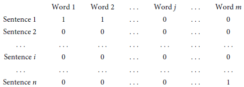
As can be seen, a DTM presents each word as one vector $W_j = (1, 0, 1, \ldots, 0, 0)$
that helps to calculate the sentiment for the next steps.
$W_j = (1, 0, 1, \ldots, 0, 0)$
that helps to calculate the sentiment for the next steps.
3.2 Dictionary-based approach
The dictionary-based method (or lexicon-based method) is one of the most common, yet efficient methods to measure sentiment scores. A dictionary usually contains a specific list of words and can be categorized into different groups. The dictionary would search for the exact word or synonyms in the window of the target words, assign a value for each word that appeared, and categorize them (Grimmer and Stewart, Reference Grimmer and Stewart2013). We intend to measure the tone of the ECB documents and classify them as hawkish or dovish.Footnote
8
Assume that a value $s_{ij} =1$
will be assigned if the target word is associated with a hawkish word and
$s_{ij} =1$
will be assigned if the target word is associated with a hawkish word and $s_{ij}=0$
if there is no hawkish word associated with the target word. Then the total hawkish score of one document is calculated as follows:
$s_{ij}=0$
if there is no hawkish word associated with the target word. Then the total hawkish score of one document is calculated as follows:
 \begin{equation} t_{hawkish} = \displaystyle \sum _{i=1}^{n} \displaystyle \sum _{j=1}^{m} \frac {s_{ij} W_{ij}}{N_i}, \end{equation}
where $W_{ij}$
is the count of a target word
$W_{ij}$
is the count of a target word $j$
appearing in sentence
$j$
appearing in sentence $i$
, and
$i$
, and $N_i$
is the total number of words used in sentence
$N_i$
is the total number of words used in sentence $i$
. Similarly, we apply the same method to measure the dovish scores. The final sentiment score is the difference between the hawkish and dovish scores of each document:
$i$
. Similarly, we apply the same method to measure the dovish scores. The final sentiment score is the difference between the hawkish and dovish scores of each document:
 \begin{equation} t_{sentiment} = t_{hawkish} - t_{dovish}. \end{equation}
Several authors have already pointed out that applying a general dictionary for specific topics could lead to misspecification of the tone of a document (Grimmer and Stewart, Reference Grimmer and Stewart2013; Picault and Renault, Reference Picault and Renault2017). The Lexicoder sentiment dictionary (LSD) and the Loughran and McDonald (Reference Loughran and McDonald2011) dictionary are perhaps the two most popular off-the-shelf dictionaries applied to natural processing language. Both contain word lists for negative and positive categories. In addition, LSD provides word lists of negate negative (such as not a lie, not abnormal*, etc.) and negate positive (such as better not, not able, etc.) categories. According to Loughran and McDonald (Reference Loughran and McDonald2011), almost three-quarters (73.8%) of the negative words following the Harvard list are words that do not have a negative meaning in a financial context. An alternative way to minimize this problem is to use an organic dictionary. We follow this solution because there is no dictionary that contains the hawkish and dovish categories, which would be necessary in our sentiment analysis. The word list of our dictionary is based on the vocabulary of the ECB press conferences and a comprehensive review of previous organic dictionaries on the same topics (Picault and Renault, Reference Picault and Renault2017; Máté et al. Reference Máté, Sebők and Barczikay2021). Thus, our dictionary contains words (bi-grams) of macroeconomic topics including “inflation”, “interest rate”, and “unemployment”. For each keyword, we develop a list of hawkish words and dovish words, respectively. For example, interest rate + increase is categorized as hawkish and vice versa (see Table A1 in Appendix A for details). As the dictionary is designed only for monetary policy topics, we can easily validate sentiment scores. Using this approach, we basically follow Zipf’s principle of least effort (Zipf, Reference Zipf2016). Harvard linguist George Kingsley Zipf was interested in human behavior when using languages. His study showed evidence that the frequency of the term is inversely proportional to its rank in a document. Therefore, we rely on a parsimonious set of words focusing on the most relevant macroeconomic topics.
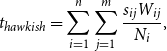
To give further insight of how the sentiment is measured, consider this sentence:
”Inflation remains very low in the context of weak demand and significant slack in labour and product markets.”
European Central Bank (ECB 2025)
The list of target words will be collected for the first step (see Table A1 for the list of target words). In this case, only the target word “inflation” will be considered. Next, the window of “inflation” is narrowed down to 10 words before and after, and all stop words are eliminated, which results in the total number of words $N=6$
. Since “inflation” only appears once,
$N=6$
. Since “inflation” only appears once, $W_{ij} = 1$
. The word “low” is categorized as dovish, thus
$W_{ij} = 1$
. The word “low” is categorized as dovish, thus $s_{ij} = 1$
. Additionally, since the word “weak” is included in the window of “inflation”, a value of
$s_{ij} = 1$
. Additionally, since the word “weak” is included in the window of “inflation”, a value of $s_{ij} = 1$
is also assigned to “weak”. Thus, the dovish sentiment of this sentence is:
$s_{ij} = 1$
is also assigned to “weak”. Thus, the dovish sentiment of this sentence is:
 \begin{equation} t_{dovish} = \displaystyle \sum _{i=1}^{n} \displaystyle \sum _{j=1}^{m} \frac {s_{ij} W_{ij}}{N_i} = \displaystyle \frac {1\times 1 + 1\times 1}{6} = 0.33. \end{equation}
As there are no hawkish words in this sentence, the hawkish sentiment is equal to 0. In total, the sentiment score for this sentence is:
 \begin{equation} t_{sentiment} = t_{hawkish} - t_{dovish} = 0- 0.33 = -0.33. \end{equation}
In the final step, the sentiment of one document is the sum of all sentences’ sentiments $t_{sentiment}$
. This approach has been applied to each of the three categories (i.e., inflation, interest rate, and unemployment) separately and is then also aggregated into an overall sentiment measure by using the sum across all categories.
$t_{sentiment}$
. This approach has been applied to each of the three categories (i.e., inflation, interest rate, and unemployment) separately and is then also aggregated into an overall sentiment measure by using the sum across all categories.
3.3 ECB press conferences
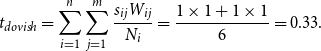
We focus on the ECB press conferences published on their website (https://www.ecb.europa.eu/press/pubbydate/html/index.en.html). The ECB press conferences contain the policy decisions after each Governing Council meeting and mainly inform the public about key interest rates, economic activity, and inflation. At the end of the press conference, there is an Q&A part, which clarifies some specific aspects and provides more information. Usually, every six weeks, the ECB releases its monetary policy decisions, statements, and Q&A. Overall, we collected 266 press conferences from 09/06/1998 to 08/09/2022 with a mean word count of 5,719 words. One benefit of using press conferences, instead of the monetary decisions or the monetary policy accounts, which are also published separately, is that the press conferences explain the decisions in more detail while also describing the overall environment. The length and size of each press conference are also adequate to classify the tone of the document. In contrast, monetary decisions are usually brief and neutral. Table A2 provided in Appendix B shows two paragraphs extracted from the ECB policy decision and the ECB press conference on 06/03/2014. As can be seen, in addition to stating the decisions from the Governing Council meeting, the press conference explained why the Governing Council did not change the interest rate on the marginal lending facility and the deposit facility (”moderate recovery of the euro area” and “a prolonged period of low inflation”). It is easy to detect some dovish words such as “moderate”, “low”, etc. associated with the main ECB topics such as “economy” and “inflation”. Figure 1 shows the top 20 words used in ECB press conferences. The main topics are key interest rates, inflation, and the economy. This is in line with the study by Bohl et al. (Reference Bohl, Kanelis and Siklos2023), in which conventional monetary policy is associated with the words “monetari”, “stabil”, “price”, and “euro”, and unconventional monetary policy is linked to the words “inflat”, “rate”, “bank”, and “term”.
The frequency of words appearing in ECB press conferences.
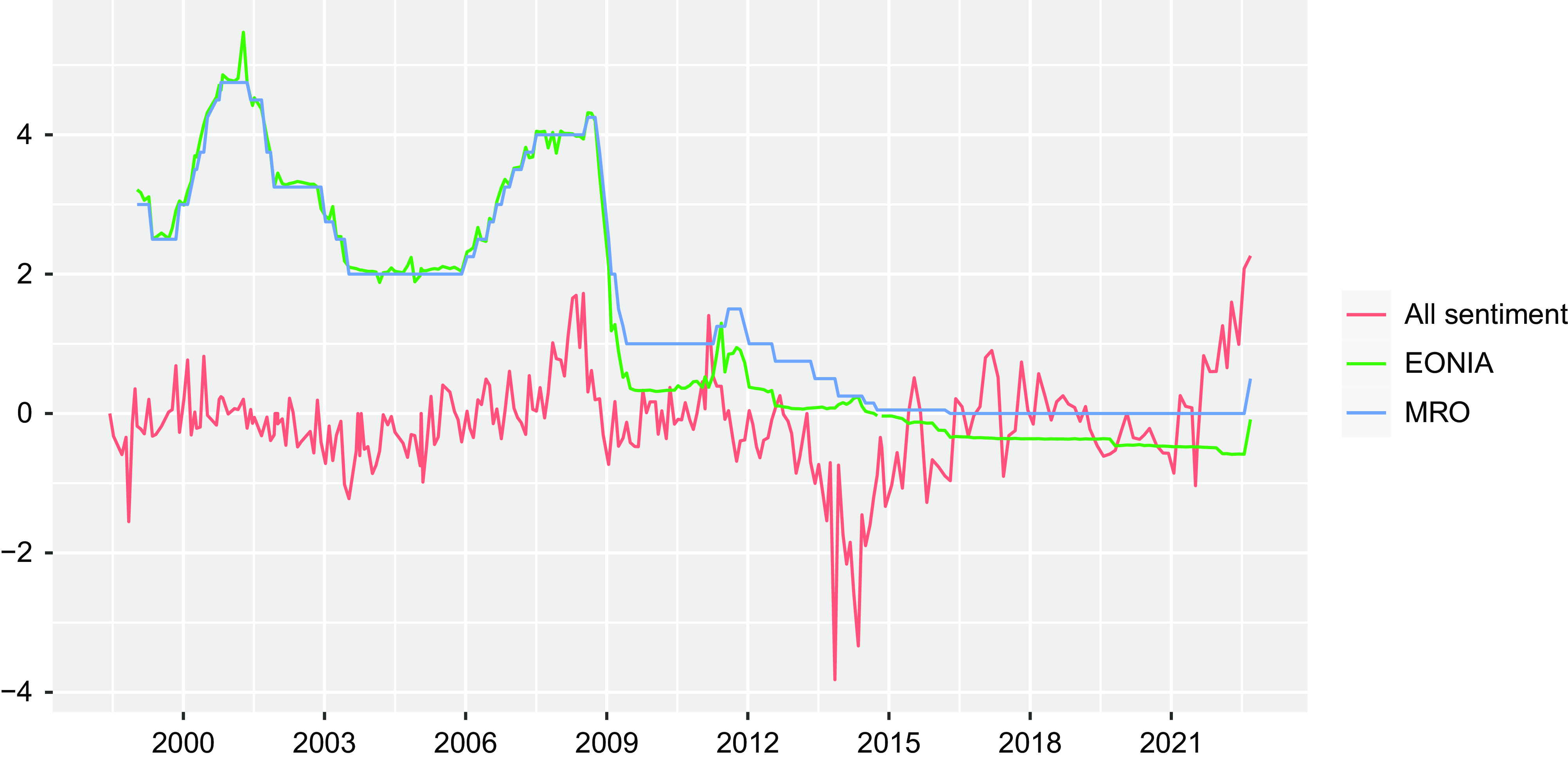
The overall sentiment score extracted from the ECB press conferences as described above is shown in Figure 2 as a red line. It is plotted against the actual policy rate of the ECB, i.e. the main refinancing operations (MRO) rate, and the interbank interest rate targeted by the ECB.Footnote 9 Overall, Figure 2 indicates that the policy rate itself characterizes the general stance of monetary policy, but the sentiment extracted from press conferences seems to offer a leading indicator function. In particular, substantial changes in the stance of monetary policy seem to be indicated earlier by the tone in press conferences before the actual policy rate is changed. This is shown for the strong interest rate cut around 2008 and 2009, for the beginning of the period of ultra-low interest rates, and also for the most recent tightening of monetary policy. In addition, Figure 2 appears to indicate that sentiment appeared to be quite hawkish around 2008 (i.e., during the global financial crisis), around 2011 (i.e., during the European debt crisis) and especially during the most recent high inflation period that started in 2021. The most dovish sentiment is observed at the start of the period of extremely low interest rates around the year 2014, where policy rates have been lowered substantially and unconventional monetary policy measures (including forward guidance) have been adopted.
Sentiment score extracted from the ECB press conferences.Note: The plot visualizes the sentiment score extracted from the ECB press conferences (red line) from June 1998 to September 2022 plotted together with the main refinancing operations (MRO) rate and the Euro Overnight Index Average (EONIA) rate at the day of the press conference.
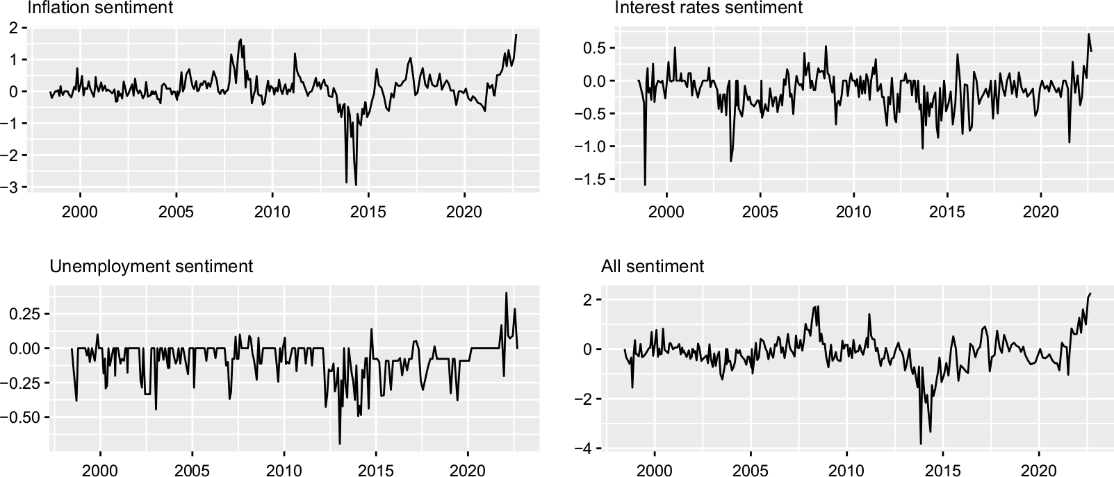
The sentiment scores for each individual keyword (i.e., inflation, interest rate, and unemployment) displayed in Figure 3 give more insight into the tone of the ECB press conferences referring to different variables. Since inflation and interest rates are the main issues discussed by the ECB, we can extract more words for them, and they exhibit more variation as well as a larger interval (i.e., from −3 to 2 for inflation and from −1.5 to 1 for interest rates) than for the sentiment of unemployment (see also the descriptive statistics provided in Table A3 in Appendix B). Thus, the aggregated sentiment measure already shown in Figure 2 is mainly driven by the sentiment referring to inflation, which is also shown by the correlation between the three individual measures and the aggregated sentiment series (see Table A4 in Appendix B).Footnote 10 The sentiment of unemployment shows much less variation and seems to be mostly dovish during the sample period. Mentioning the unemployment rate in the ECB press conferences is more often associated with expansionary monetary policy, indicating a dovish tone, which becomes most evident around the year 2013.
Sentiment scores based on keywords.
3.4 Interest rate data
Our empirical analysis starts by assessing whether the tone of central bank communication captured by our sentiment series offers any genuine news beyond actual interest rate changes. The data necessary for the EONIA, the €STR, and the MRO rate plotted in Figure 2 are taken from the ECB statistics sourced through Federal Reserve Economic Data (FRED). The interest rate data is available on a daily frequency and has been matched with the exact date stamps of the ECB press conferences used to construct the sentiments. Therefore, the data frequency refers to the frequency of ECB press conferences, which are usually held every six weeks. As already mentioned above, the €STR has been used to extend the EONIA series since January 2022. To get a continuous series for the MRO rate, we have put together the fixed tender rate, which has been used until June 2000 and since October 2008, and the minimum bid rate for the variable tender, which has been used between June 2000 and October 2008. As a sensitivity check allowing for the negative interest rate policy period, we have replaced the MRO rate by the deposit facility rate, i.e. the interest rate banks receive for holding overnight deposits at the central bank. The deposit facility rate is the lower limit of the corridor for the interbank interest rate targeted by the ECB and was negative between June 2014 and July 2022.
3.5 ECB survey of professional forecasters
For the second and third part of the empirical analysis, we rely on data taken from the ECB Survey of Professional Forecasters (ECB-SPF) for the quarterly sample period from 1999Q1 to 2022Q4. We consider individual fixed-horizon point forecasts and density forecasts for the inflation rate for the Euro Area. These forecasts have been made at the beginning of each quarter by various forecasters representing professional institutions (i.e., major banks and research institutes across the whole Euro Area). Fixed-horizon forecasts are provided for horizons of one-year-ahead, two-years-ahead, and five-years-ahead ( $h=1,2,5$
) and therefore allow for a comparison between short-term expectations (
$h=1,2,5$
) and therefore allow for a comparison between short-term expectations ( $h=1,2$
) and medium-term expectations (
$h=1,2$
) and medium-term expectations ( $h=5$
). For each horizon, we have computed cross-sectional means of inflation expectations across all forecasters at each point in time as a general measure of inflation expectations and cross-sectional standard deviations across all forecasters as a measure of disagreement among forecasters. In addition, we have also used individual density forecasts to estimate the standard deviation relying on the mass-at-midpoint approach following Abel et al. (Reference Abel, Rich, Song and Tracy2016) and Glas and Hartmann (Reference Glas and Hartmann2022) as an individual measure of uncertainty regarding future inflation.Footnote
11
Then, we have also taken cross-sectional means of the individual standard deviations. To also get a measure of heavy-tailness indicating the probability of an ‘inflation disasters’ considered by Hilscher et al. (Reference Hilscher, Raviv and Reis2022), we have also used the individual density forecasts to estimate the kurtosis applying the same approach as for the standard deviation.
$h=5$
). For each horizon, we have computed cross-sectional means of inflation expectations across all forecasters at each point in time as a general measure of inflation expectations and cross-sectional standard deviations across all forecasters as a measure of disagreement among forecasters. In addition, we have also used individual density forecasts to estimate the standard deviation relying on the mass-at-midpoint approach following Abel et al. (Reference Abel, Rich, Song and Tracy2016) and Glas and Hartmann (Reference Glas and Hartmann2022) as an individual measure of uncertainty regarding future inflation.Footnote
11
Then, we have also taken cross-sectional means of the individual standard deviations. To also get a measure of heavy-tailness indicating the probability of an ‘inflation disasters’ considered by Hilscher et al. (Reference Hilscher, Raviv and Reis2022), we have also used the individual density forecasts to estimate the kurtosis applying the same approach as for the standard deviation.
Furthermore, the ECB-SPF also includes individual point forecasts for the MRO rate for one-, two-, three-, and four-quarters-ahead, which have been included into the survey since 2002 as part of the so-called assumptions. We also compute cross-sectional means and standard deviations of these point forecasts across forecasters. Unfortunately, density forecasts are not provided for the MRO rate forecasts. Therefore, an uncertainty measure regarding the MRO rate, which might be interpreted as uncertainty regarding the stance of monetary policy, has to be constructed as follows. In line with Lahiri and Sheng (Reference Lahiri and Sheng2010), we take the sum of ex-ante uncertainty proxied by the cross-sectional standard deviation across forecasters and ex-post uncertainty. The latter is computed by the volatility of ex-post forecast errors for the MRO rate forecasts, i.e. the difference between forecasts and actual realizations of the MRO rate. Volatility is estimated by fitting a stochastic volatility model following Istrefi and Mouabbi (Reference Istrefi and Mouabbi2018) and Beckmann and Czudaj (Reference Beckmann and Czudaj2023).
4. Empirical findings
In this section, we present and discuss the results of our empirical analysis, which consists of different steps. First, we start with the following baseline predictive regression:
 \begin{equation} EONIA_t = \beta _0 + \beta _1 X_{t-k} + \epsilon _t, \end{equation}
for which we regress the interbank interest rate ( $EONIA_t$
) on different lags of our constructed sentiment measures (
$EONIA_t$
) on different lags of our constructed sentiment measures ( $X_{t-k}$
for
$X_{t-k}$
for $k=0,1,\ldots, 12$
). We basically assess whether the tone of central bank communication captured by our sentiment series predicts the interbank interest rate and whether the direction of the effect is in line with the tone of the policy communication by the ECB. We particularly focus on the interbank market, as it basically acts as the operational target of the ECB at the beginning of the transmission mechanism of the monetary policy by the ECB.Footnote
12
The variable of interest is
$k=0,1,\ldots, 12$
). We basically assess whether the tone of central bank communication captured by our sentiment series predicts the interbank interest rate and whether the direction of the effect is in line with the tone of the policy communication by the ECB. We particularly focus on the interbank market, as it basically acts as the operational target of the ECB at the beginning of the transmission mechanism of the monetary policy by the ECB.Footnote
12
The variable of interest is $X_{t-k}$
, which represents our different sentiment measures (that is, inflation sentiment, interest rate sentiment, unemployment sentiment, and aggregated sentiment as illustrated in Figure 3). The corresponding coefficient estimates are shown in Figure 4 together with their 95% confidence intervals based on heteroscedasticity-and-autocorrelation-consistent (HAC) standard errors.
$X_{t-k}$
, which represents our different sentiment measures (that is, inflation sentiment, interest rate sentiment, unemployment sentiment, and aggregated sentiment as illustrated in Figure 3). The corresponding coefficient estimates are shown in Figure 4 together with their 95% confidence intervals based on heteroscedasticity-and-autocorrelation-consistent (HAC) standard errors.
Effect of sentiment based on keywords on interbank interest rates.
Note: The plot shows the estimated $\beta _1$
coefficient of the following regression:
$\beta _1$
coefficient of the following regression:
 \begin{equation*} EONIA_t = \beta _0 + \beta _1 X_{t-k} + \epsilon _t, \end{equation*}
where $EONIA_t$
denotes the interbank interest rate and
$EONIA_t$
denotes the interbank interest rate and $X_{t-k}$
is the constructed sentiment measure from ECB press conferences for different lags
$X_{t-k}$
is the constructed sentiment measure from ECB press conferences for different lags $k=0,1,\ldots, 12$
. The points provide coefficient estimates and the whiskers indicate heteroscedasticity-and-autocorrelation-consistent (HAC) standard errors multiplied with the 97.5% quantiles of the standard normal distribution. The dashed black line is the zero line and the red line displays the adjusted
$k=0,1,\ldots, 12$
. The points provide coefficient estimates and the whiskers indicate heteroscedasticity-and-autocorrelation-consistent (HAC) standard errors multiplied with the 97.5% quantiles of the standard normal distribution. The dashed black line is the zero line and the red line displays the adjusted $R^2$
.
$R^2$
.
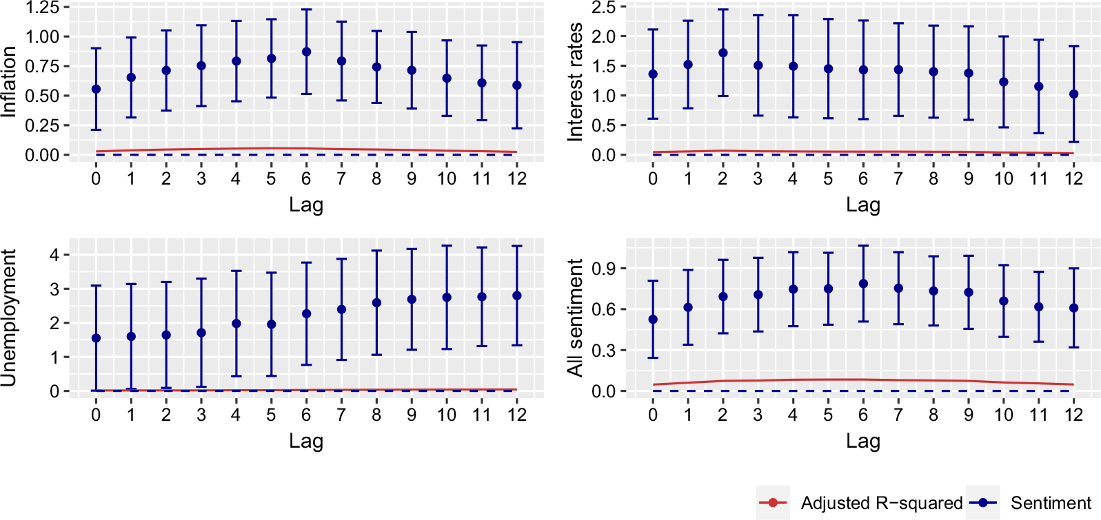
As can be seen in Figure 4, hawkishness in the four considered sentiments, which can be interpreted as an increase in interest rates, has the expected positive effect on interbank interest rates and is clearly significant for nearly all considered lags of the four sentiments.Footnote
13
This is first evidence that the tone of central bank communication by the ECB is capable of predicting the interbank market and that the direction of the tone has been appropriately characterized by our approach as hawkishness seems to increase interbank interest rates, which is also in line with the evidence by Picault and Renault (Reference Picault and Renault2017). In the following, we also examine whether the tone of central bank communication captured by our sentiment series offers any genuine news beyond actual policy rate changes. In doing so, we extend the predictive regression above by the ECB policy rate (that is, the main refinancing operations rate) denoted as $MRO_t$
, which acts as a control variable here:Footnote
14
$MRO_t$
, which acts as a control variable here:Footnote
14
 \begin{equation} EONIA_t = \beta _0 + \beta _1 X_{t-k} + \beta _2 MRO_t + \epsilon _t. \end{equation}
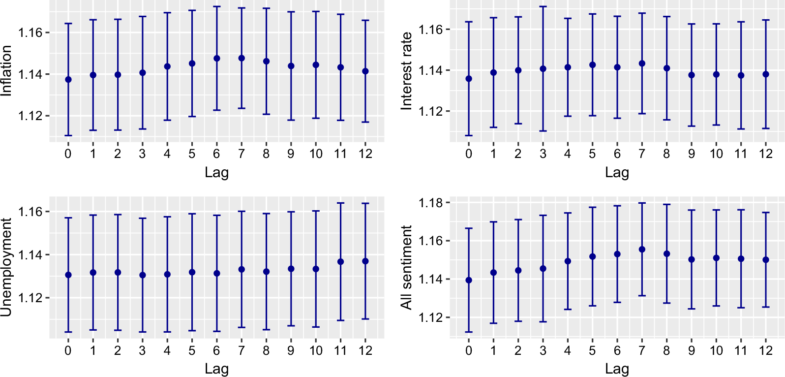
Estimates of the corresponding coefficients are visualized in Figures 5 and 6. Figure 5 illustrates the estimated interest rate pass-through coefficient ( $\beta _2$
) across the different specifications (i.e.,
$\beta _2$
) across the different specifications (i.e., $k=0,1,\ldots, 12$
) showing how the policy rate passes through to the interbank interest rate, which is targeted by the ECB. The interest rate pass-through coefficient is around 1.14 across the different specifications and is significantly different from zero, which shows that the transmission from the policy rate to the interbank rate generally works fine. The pass-through is even slightly above unity, which indicates a slight overreaction of the market on policy rate decision days. The adjusted
$k=0,1,\ldots, 12$
) showing how the policy rate passes through to the interbank interest rate, which is targeted by the ECB. The interest rate pass-through coefficient is around 1.14 across the different specifications and is significantly different from zero, which shows that the transmission from the policy rate to the interbank rate generally works fine. The pass-through is even slightly above unity, which indicates a slight overreaction of the market on policy rate decision days. The adjusted $R^2$
is around 0.98 for all specifications and underscores a very close relationship between both interest rates.
$R^2$
is around 0.98 for all specifications and underscores a very close relationship between both interest rates.
Interest rate pass-through coefficient of the policy rate (MRO).
Note: The plot shows the estimated $\beta _2$
coefficient of the following regression:
$\beta _2$
coefficient of the following regression:
 \begin{equation*} EONIA_t = \beta _0 + \beta _1 X_{t-k} + \beta _2 MRO_t + \epsilon _t, \end{equation*}
where $EONIA_t$
denotes the interbank interest rate,
$EONIA_t$
denotes the interbank interest rate, $X_{t-k}$
is the constructed sentiment measure from ECB press conferences for different lags
$X_{t-k}$
is the constructed sentiment measure from ECB press conferences for different lags $k=0,1,\ldots, 12$
, and
$k=0,1,\ldots, 12$
, and $MRO_t$
stands for the policy rate of the ECB (main refinancing operations rate). The points provide coefficient estimates and the whiskers indicate heteroscedasticity-and-autocorrelation-consistent (HAC) standard errors multiplied with the 97.5% quantiles of the standard normal distribution.
$MRO_t$
stands for the policy rate of the ECB (main refinancing operations rate). The points provide coefficient estimates and the whiskers indicate heteroscedasticity-and-autocorrelation-consistent (HAC) standard errors multiplied with the 97.5% quantiles of the standard normal distribution.
Effect of sentiment based on keywords on interbank interest rates.
Note: The plot shows the estimated $\beta _1$
coefficient of the following regression:
$\beta _1$
coefficient of the following regression:
 \begin{equation*} EONIA_t = \beta _0 + \beta _1 X_{t-k} + \beta _2 MRO_t + \epsilon _t, \end{equation*}
where $EONIA_t$
denotes the interbank interest rate,
$EONIA_t$
denotes the interbank interest rate, $X_{t-k}$
is the constructed sentiment measure from ECB press conferences for different lags
$X_{t-k}$
is the constructed sentiment measure from ECB press conferences for different lags $k=0,1,\ldots, 12$
, and
$k=0,1,\ldots, 12$
, and $MRO_t$
stands for the policy rate of the ECB (main refinancing operations rate). The points provide coefficient estimates and the whiskers indicate heteroscedasticity-and-autocorrelation-consistent (HAC) standard errors multiplied with the 97.5% quantiles of the standard normal distribution. The dashed black line is the zero line. The adjusted
$MRO_t$
stands for the policy rate of the ECB (main refinancing operations rate). The points provide coefficient estimates and the whiskers indicate heteroscedasticity-and-autocorrelation-consistent (HAC) standard errors multiplied with the 97.5% quantiles of the standard normal distribution. The dashed black line is the zero line. The adjusted $R^2$
in all regressions lies between 0.982 to 0.985.
$R^2$
in all regressions lies between 0.982 to 0.985.

Figure 6 provides the sentiment coefficient ( $\beta _1$
) for the different sentiments and the various lags
$\beta _1$
) for the different sentiments and the various lags $k=0,1,\ldots, 12$
together with their 95% confidence intervals based on HAC standard errors. Focusing on inflation and interest rate sentiments (graphs in the first row of Figure 6), we clearly see a significantly negative sentiment predictability that goes beyond the information already provided in the policy rate decision. When considering the fact that we find a small overreaction in the interest rate pass-through mentioned above, the negative sentiment coefficients are plausible. These act as some kind of correction for the overreaction. This becomes evident as the magnitude of the sentiment coefficients is very similar to the deviation of the pass-through coefficients from unity. As the sum of both coefficient estimates (i.e.,
$k=0,1,\ldots, 12$
together with their 95% confidence intervals based on HAC standard errors. Focusing on inflation and interest rate sentiments (graphs in the first row of Figure 6), we clearly see a significantly negative sentiment predictability that goes beyond the information already provided in the policy rate decision. When considering the fact that we find a small overreaction in the interest rate pass-through mentioned above, the negative sentiment coefficients are plausible. These act as some kind of correction for the overreaction. This becomes evident as the magnitude of the sentiment coefficients is very similar to the deviation of the pass-through coefficients from unity. As the sum of both coefficient estimates (i.e., $\beta _1$
and
$\beta _1$
and $\beta _2$
) is roughly close to unity, the pass-through to the interbank interest rate may be split into a part induced by the actual policy rate change and a part that can be traced back to monetary policy communication. The results for the unemployment sentiment are less clear, but we also find coefficients significantly below zero for the lags above 8. In general, we provide robust evidence that the ECB’s communication policy and its tone play a role in the transmission process of monetary policy, which is especially indicated by the significant effect of the aggregated sentiment measure.Footnote
15
It also becomes evident that sentiments have a higher predictability for actual interest rate changes over lags of around 6 and above. This finding is intuitive because of the observation that monetary policy communication is often used to (at least implicitly) indicate potential policy changes much earlier than they are actually executed to manage expectations of market participants. The corresponding findings generally continue to hold, when replacing the main refinancing operations rate (
$\beta _2$
) is roughly close to unity, the pass-through to the interbank interest rate may be split into a part induced by the actual policy rate change and a part that can be traced back to monetary policy communication. The results for the unemployment sentiment are less clear, but we also find coefficients significantly below zero for the lags above 8. In general, we provide robust evidence that the ECB’s communication policy and its tone play a role in the transmission process of monetary policy, which is especially indicated by the significant effect of the aggregated sentiment measure.Footnote
15
It also becomes evident that sentiments have a higher predictability for actual interest rate changes over lags of around 6 and above. This finding is intuitive because of the observation that monetary policy communication is often used to (at least implicitly) indicate potential policy changes much earlier than they are actually executed to manage expectations of market participants. The corresponding findings generally continue to hold, when replacing the main refinancing operations rate ( $MRO_t$
) in Eq. (6) by the deposit facility rate as the main policy rate. This robustness check intends to account for the long period of zero interest rate policy followed by the ECB, in which the main refinancing operations rate was zero between 2016 and 2022 (see Figure 2). Within this period the interbank interest rate turned into negative lying quite close to the deposit facility rate. The corresponding findings for this robustness check are shown in Figures A1 and A2 in Appendix D and basically confirm the findings discussed above.
$MRO_t$
) in Eq. (6) by the deposit facility rate as the main policy rate. This robustness check intends to account for the long period of zero interest rate policy followed by the ECB, in which the main refinancing operations rate was zero between 2016 and 2022 (see Figure 2). Within this period the interbank interest rate turned into negative lying quite close to the deposit facility rate. The corresponding findings for this robustness check are shown in Figures A1 and A2 in Appendix D and basically confirm the findings discussed above.
As a next step of our analysis, to shed further light on the monetary policy transmission of the communication by the ECB, we also analyze the predictability of our sentiments on inflation expectations taken from the ECB Survey of Professional Forecasters (ECB-SPF). In doing so, we rely on a similar approach and estimate the following predictive regression:Footnote 16
 \begin{equation} Y_{t,h} = \beta _0 + \beta _1 X_{t-k} + \beta _2 MRO_t + \epsilon _t, \end{equation}
where $Y_{t,h}$
denotes mean inflation expectations across professionals, the disagreement among professionals (i.e., the cross-sectional standard deviation across forecasters), the mean forecasters’ uncertainty regarding future inflation (i.e., the cross-sectional mean of the individual standard deviations of the density forecasts), or the mean kurtosis of the density forecasts across three different horizons (i.e., one-, two-, and five-years-ahead given by
$Y_{t,h}$
denotes mean inflation expectations across professionals, the disagreement among professionals (i.e., the cross-sectional standard deviation across forecasters), the mean forecasters’ uncertainty regarding future inflation (i.e., the cross-sectional mean of the individual standard deviations of the density forecasts), or the mean kurtosis of the density forecasts across three different horizons (i.e., one-, two-, and five-years-ahead given by $h=1,2,5$
).
$h=1,2,5$
). $X_{t-k}$
again represents our sentiment scores across different lags
$X_{t-k}$
again represents our sentiment scores across different lags $k=0,1,\ldots, 12$
, which are now measured at a quarterly frequency to match the data frequency of the ECB-SPF.Footnote
17
In this case we have solely considered inflation and interest rate sentiments and have omitted the unemployment sentiment due to inconclusive results in the previous step. The estimates of the corresponding sentiment coefficient for
$k=0,1,\ldots, 12$
, which are now measured at a quarterly frequency to match the data frequency of the ECB-SPF.Footnote
17
In this case we have solely considered inflation and interest rate sentiments and have omitted the unemployment sentiment due to inconclusive results in the previous step. The estimates of the corresponding sentiment coefficient for $\beta _1$
are shown in Figures 7 and 8.
$\beta _1$
are shown in Figures 7 and 8.
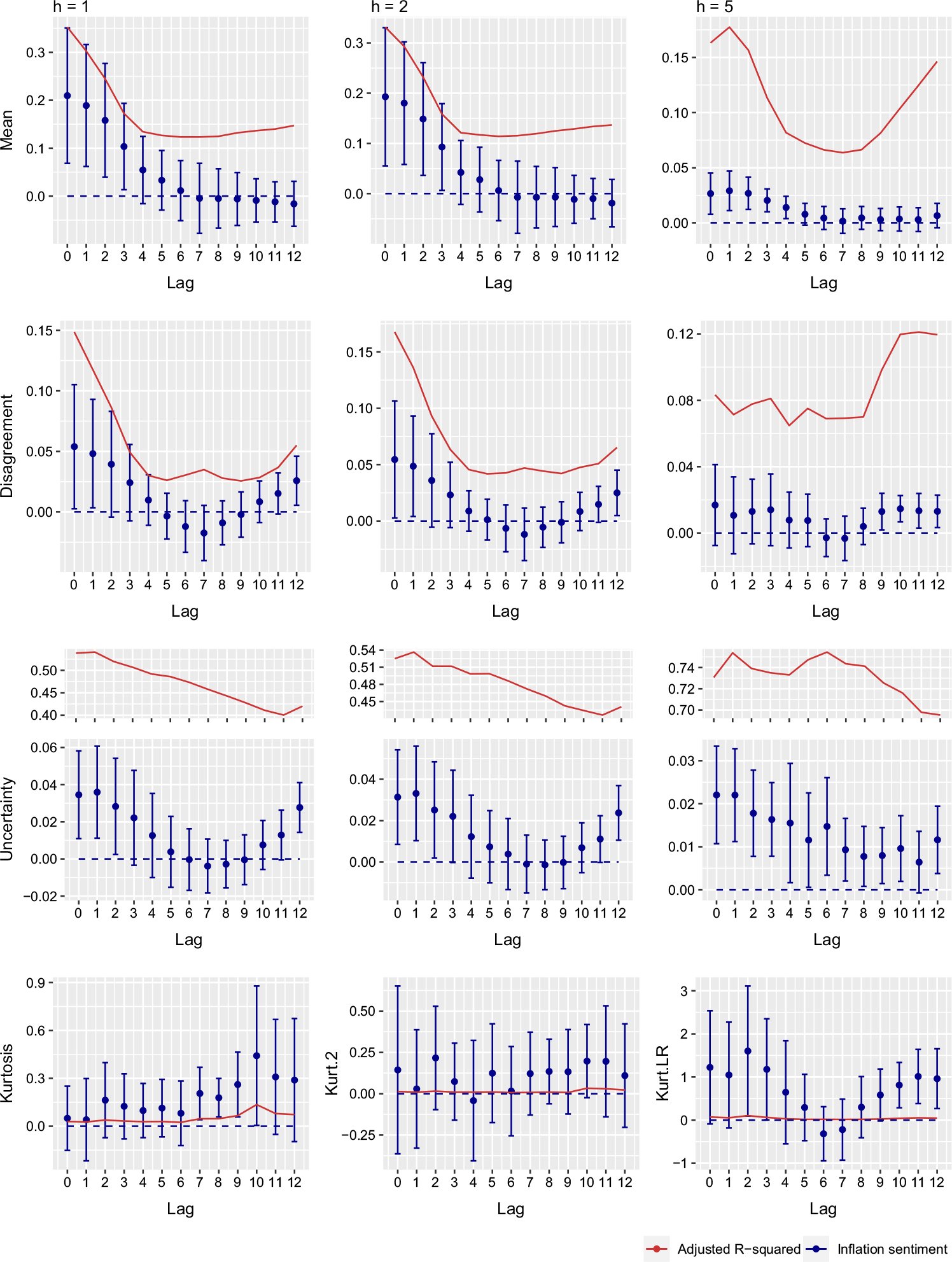
Effect of inflation sentiment on inflation expectation.
Note: The plot shows the estimated $\beta _1$
coefficient of the following regression:
$\beta _1$
coefficient of the following regression:
 \begin{equation*} Y_{t,h} = \beta _0 + \beta _1 X_{t-k} + \beta _2 MRO_t + \epsilon _t, \end{equation*}
where $Y_{t,h}$
denotes mean inflation expectations across professionals, the disagreement among professionals (i.e., the cross-sectional standard deviation across forecasters), the mean forecasters’ uncertainty regarding future inflation (i.e., the cross-sectional mean of the individual standard deviations of the density forecasts), or the mean kurtosis of the density forecasts across three different horizons (i.e., one-, two-, and five-years-ahead given by
$Y_{t,h}$
denotes mean inflation expectations across professionals, the disagreement among professionals (i.e., the cross-sectional standard deviation across forecasters), the mean forecasters’ uncertainty regarding future inflation (i.e., the cross-sectional mean of the individual standard deviations of the density forecasts), or the mean kurtosis of the density forecasts across three different horizons (i.e., one-, two-, and five-years-ahead given by $h=1,2,5$
).
$h=1,2,5$
). $X_{t-k}$
is the constructed inflation sentiment measure from ECB press conferences for different lags
$X_{t-k}$
is the constructed inflation sentiment measure from ECB press conferences for different lags $k=0,1,\ldots, 12$
and
$k=0,1,\ldots, 12$
and $MRO_t$
stands for the policy rate of the ECB (main refinancing operations rate). The points provide coefficient estimates and the whiskers indicate heteroscedasticity-and-autocorrelation-consistent (HAC) standard errors multiplied with the 97.5% quantiles of the standard normal distribution. The red line represents the adjusted
$MRO_t$
stands for the policy rate of the ECB (main refinancing operations rate). The points provide coefficient estimates and the whiskers indicate heteroscedasticity-and-autocorrelation-consistent (HAC) standard errors multiplied with the 97.5% quantiles of the standard normal distribution. The red line represents the adjusted $R^2$
.
$R^2$
.
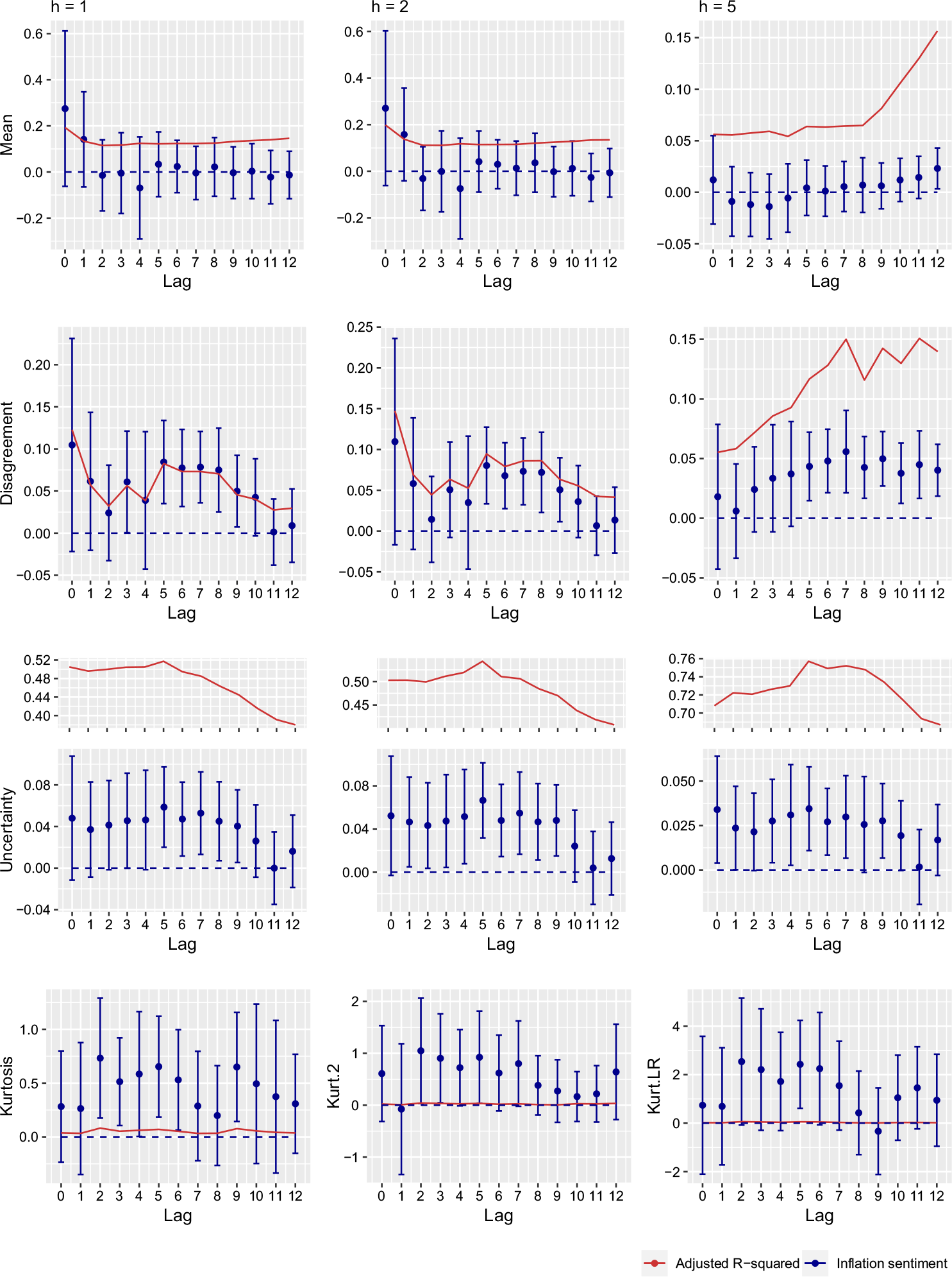
Effect of interest rate sentiment on inflation expectation.
Note: The plot shows the estimated $\beta _1$
coefficient of the following regression:
$\beta _1$
coefficient of the following regression:
 \begin{equation*} Y_{t,h} = \beta _0 + \beta _1 X_{t-k} + \beta _2 MRO_t + \epsilon _t, \end{equation*}
where $Y_{t,h}$
denotes mean inflation expectations across professionals, the disagreement among professionals (i.e., the cross-sectional standard deviation across forecasters), the mean forecasters’ uncertainty regarding future inflation (i.e., the cross-sectional mean of the individual standard deviations of the density forecasts), or the mean kurtosis of the density forecasts across three different horizons (i.e., one-, two-, and five-years-ahead given by
$Y_{t,h}$
denotes mean inflation expectations across professionals, the disagreement among professionals (i.e., the cross-sectional standard deviation across forecasters), the mean forecasters’ uncertainty regarding future inflation (i.e., the cross-sectional mean of the individual standard deviations of the density forecasts), or the mean kurtosis of the density forecasts across three different horizons (i.e., one-, two-, and five-years-ahead given by $h=1,2,5$
).
$h=1,2,5$
). $X_{t-k}$
is the constructed interest rate sentiment measure from ECB press conferences for different lags
$X_{t-k}$
is the constructed interest rate sentiment measure from ECB press conferences for different lags $k=0,1,\ldots, 12$
and
$k=0,1,\ldots, 12$
and $MRO_t$
stands for the policy rate of the ECB (main refinancing operations rate). The points provide coefficient estimates and the whiskers indicate heteroscedasticity-and-autocorrelation-consistent (HAC) standard errors multiplied with the 97.5% quantiles of the standard normal distribution. The dashed black line is the zero line. The red line represents the adjusted
$MRO_t$
stands for the policy rate of the ECB (main refinancing operations rate). The points provide coefficient estimates and the whiskers indicate heteroscedasticity-and-autocorrelation-consistent (HAC) standard errors multiplied with the 97.5% quantiles of the standard normal distribution. The dashed black line is the zero line. The red line represents the adjusted $R^2$
.
$R^2$
.
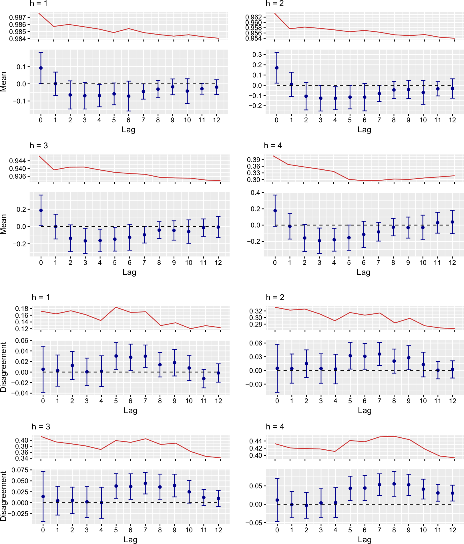
Effect of interest rates sentiment on policy rate expectations.
Note: The plot shows the estimated $\beta _1$
coefficient of the following regression:
$\beta _1$
coefficient of the following regression:
 {\begin{equation*} Y_{t,h} = \beta _0 + \beta _1 X_{t-k} + \beta _2 MRO_t + \epsilon _t, \end{equation*}
where $Y_{t,h}$
denotes mean policy rate expectations across professionals, the disagreement among professionals (i.e., the cross-sectional standard deviation across forecasters), the estimated volatility of ex-post forecast errors or monetary policy uncertainty defined as the sum of ex-ante disagreement and volatility of ex-post forecast errors across four different horizons (i.e., one-, two-, three- and four-quarters-ahead given by
$Y_{t,h}$
denotes mean policy rate expectations across professionals, the disagreement among professionals (i.e., the cross-sectional standard deviation across forecasters), the estimated volatility of ex-post forecast errors or monetary policy uncertainty defined as the sum of ex-ante disagreement and volatility of ex-post forecast errors across four different horizons (i.e., one-, two-, three- and four-quarters-ahead given by $h=1,2,3,4$
).
$h=1,2,3,4$
). $X_{t-k}$
is the constructed interest rate sentiment measure from ECB press conferences for different lags
$X_{t-k}$
is the constructed interest rate sentiment measure from ECB press conferences for different lags $k=0,1,\ldots, 12$
and
$k=0,1,\ldots, 12$
and $MRO_t$
stands for the policy rate of the ECB (main refinancing operations rate). The points provide coefficient estimates and the whiskers indicate heteroscedasticity-and-autocorrelation-consistent (HAC) standard errors multiplied with the 97.5% quantiles of the standard normal distribution. The dashed black line is the zero line. The red line represents the adjusted
$MRO_t$
stands for the policy rate of the ECB (main refinancing operations rate). The points provide coefficient estimates and the whiskers indicate heteroscedasticity-and-autocorrelation-consistent (HAC) standard errors multiplied with the 97.5% quantiles of the standard normal distribution. The dashed black line is the zero line. The red line represents the adjusted $R^2$
.
$R^2$
.
The first row of Figure 7 displays that the inflation sentiment significantly affects inflation expectations on all three horizons for the first lags (at least up to lag 3). The positive effect of hawkishness (i.e., an increase in the inflation sentiments) on inflation expectations verifies that the communication of the ECB generally plays a role for the formation of inflation expectations by professionals. The ECB aims to anchor inflation expectations at their inflation target level of 2%. This means that inflation expectations, especially for the longer term, should not react to any kind of short-term news. The significant effect of the inflation sentiment on inflation expectations across all horizons indicates that the communication strategy seems not to contribute to the anchoring of inflation expectations.Footnote 18 In the same vein, the graphs in the second and third row of Figure 7 illustrate that the inflation sentiment derived from the communication of the ECB significantly drives up disagreement and uncertainty among forecasters regarding future inflation on various lags. This finding reconciles with the existing literature. Ehrmann et al. (Reference Ehrmann, Gaballo, Hoffmann and Strasser2019) rely on a cross-country event-study approach to study whether different forms of forward guidance (i.e., open-ended, time-contingent, and state-contingent) are able to mute the effect of macroeconomic surprises on bond yields and the disagreement of forecasters regarding future interest rates and show that calendar-based forward guidance with a short horizon seems to increase the disagreement among forecasters. They rationalize the latter finding by proposing a model where agents learn from market signals, which shows that the publication of more precise information about future interest rates may lower the informativeness of market signals resulting in a rise in the level of uncertainty. This is also generally in line with the literature on information rigidity explained by sticky or noise information models (see e.g. Coibion and Gorodnichenko Reference Coibion and Gorodnichenko2015; Czudaj, Reference Czudaj2022).
The effect on the kurtosis of inflation forecasts is less clear-cut but also turns out to be significant in some cases. In general, it seems that the expectation formation behavior of professionals is significantly affected by the communication policy of the ECB. However, the latter tends to blur expectations resulting in uncertainty regarding future inflation and de-anchored inflation expectations. Figure 8 provides the corresponding results for the interest rate sentiment, which do not show any significant reaction to inflation expectations. However, we also see an significant increase in disagreement and uncertainty regarding future inflation. The overall finding of a positive association of the tone in policy communication conducted by the ECB and disagreement and/or uncertainty regarding future inflation might also be driven by the coincidence of a more hawkish tone in periods characterized by a larger uncertainty. To also control for this possibility, we have considered a sensitivity check that also includes the economic policy uncertainty (EPU) index based on the coverage of newspapers for Europe in the tradition of Baker et al. (Reference Baker, Bloom and Davis2016).Footnote 19 The corresponding findings are provided in Figures A3 and A4 in Appendix D and basically confirm our results.
As a next step, we are also interested in the connection between the interest rate sentiment and professionals’ expectations regarding the policy rate of the ECB. Therefore, we rely on the same predictive regression as given by Eq. (7) while $Y_{t,h}$
now refers to mean policy rate expectations across professionals, the disagreement among professionals (i.e., the cross-sectional standard deviation across forecasters), the estimated volatility of ex-post forecast errors or monetary policy uncertainty defined as the sum of ex-ante disagreement and volatility of ex-post forecast errors across four different horizons (i.e., one-, two-, three- and four-quarters-ahead given by
$Y_{t,h}$
now refers to mean policy rate expectations across professionals, the disagreement among professionals (i.e., the cross-sectional standard deviation across forecasters), the estimated volatility of ex-post forecast errors or monetary policy uncertainty defined as the sum of ex-ante disagreement and volatility of ex-post forecast errors across four different horizons (i.e., one-, two-, three- and four-quarters-ahead given by $h=1,2,3,4$
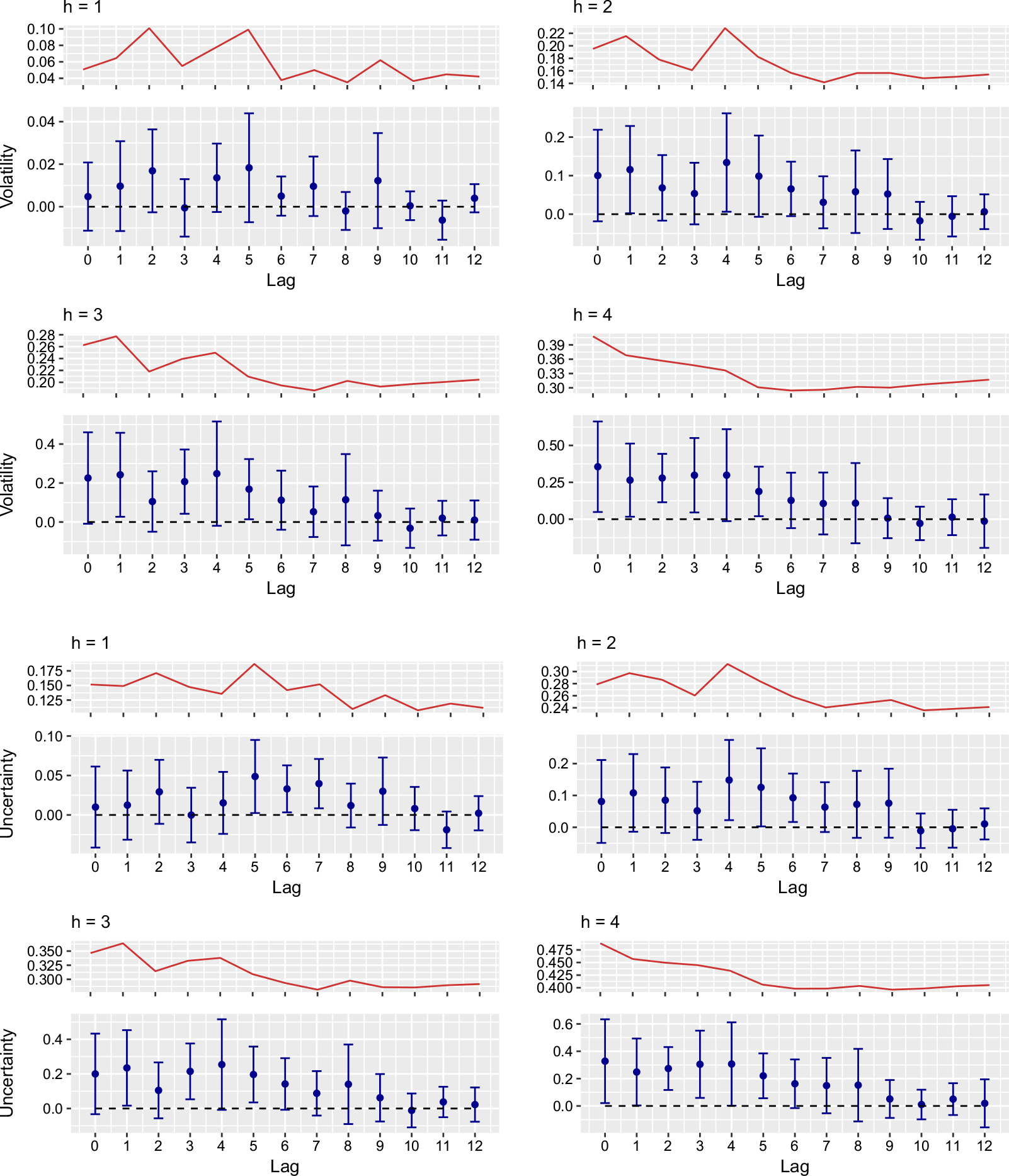
). The associated findings are shown in Figures 9 and 10. Hawkishness seems to increase policy rate expectations contemporaneously. For the higher horizons (i.e., three- and four-quarter-ahead) we also find significantly negative associations with policy rate expectations at several lags, which are in line with the effects on interbank interest rates mentioned above. The same as for inflation expectations, significantly positive predictability of the sentiment on disagreement, volatility, and uncertainty regarding the future policy rate can be observed, which indicates that the tone of central bank communication conducted by the ECB in some cases increases monetary policy uncertainty among market participants instead of lowering it.
$h=1,2,3,4$
). The associated findings are shown in Figures 9 and 10. Hawkishness seems to increase policy rate expectations contemporaneously. For the higher horizons (i.e., three- and four-quarter-ahead) we also find significantly negative associations with policy rate expectations at several lags, which are in line with the effects on interbank interest rates mentioned above. The same as for inflation expectations, significantly positive predictability of the sentiment on disagreement, volatility, and uncertainty regarding the future policy rate can be observed, which indicates that the tone of central bank communication conducted by the ECB in some cases increases monetary policy uncertainty among market participants instead of lowering it.
Effect of interest rates sentiment on policy rate expectations (Cont. from Figure 9).
Finally, we also study the effect of tone in central bank communication on the real economy. In doing so, we estimate impulse response functions based on a simple structural vector autoregression (SVAR) using a Bayesian estimation algorithm in combination with sign restrictions. We basically set up an SVAR model with two lags suggested by the Bayesian information criterion for the sample period from 1999Q1 to 2022Q3 on a quarterly level for the Euro Area with four variables: the growth rate in real gross domestic product (GDP), the inflation rate (growth in the consumer price index), the ECB policy rate (main refinancing operations rate), and the aggregated sentiment measure.Footnote 20 The sign restriction scheme adopted to identify a monetary policy communication shock, which we consider here, requires that the shock acts as a conventional monetary policy shock while again controlling for the policy rate. Therefore, we assume that the shock increases the policy rate and the sentiment (hawkishness tone) and drives down real GDP growth and inflation. The impulse response of GDP growth and inflation to the monetary policy communication shock is obtained by the rejection method algorithm proposed by Rubio-Ramírez et al. (Reference Rubio-Ramírez, Waggoner and Zha2010) until it reaches 1,000 accepted draws (see Appendix D or Rubio-Ramírez et al. (Reference Rubio-Ramírez, Waggoner and Zha2010) for details). For robustness purposes, we also consider both the rejection method and the penalty function method suggested by Uhlig (Reference Uhlig2005).
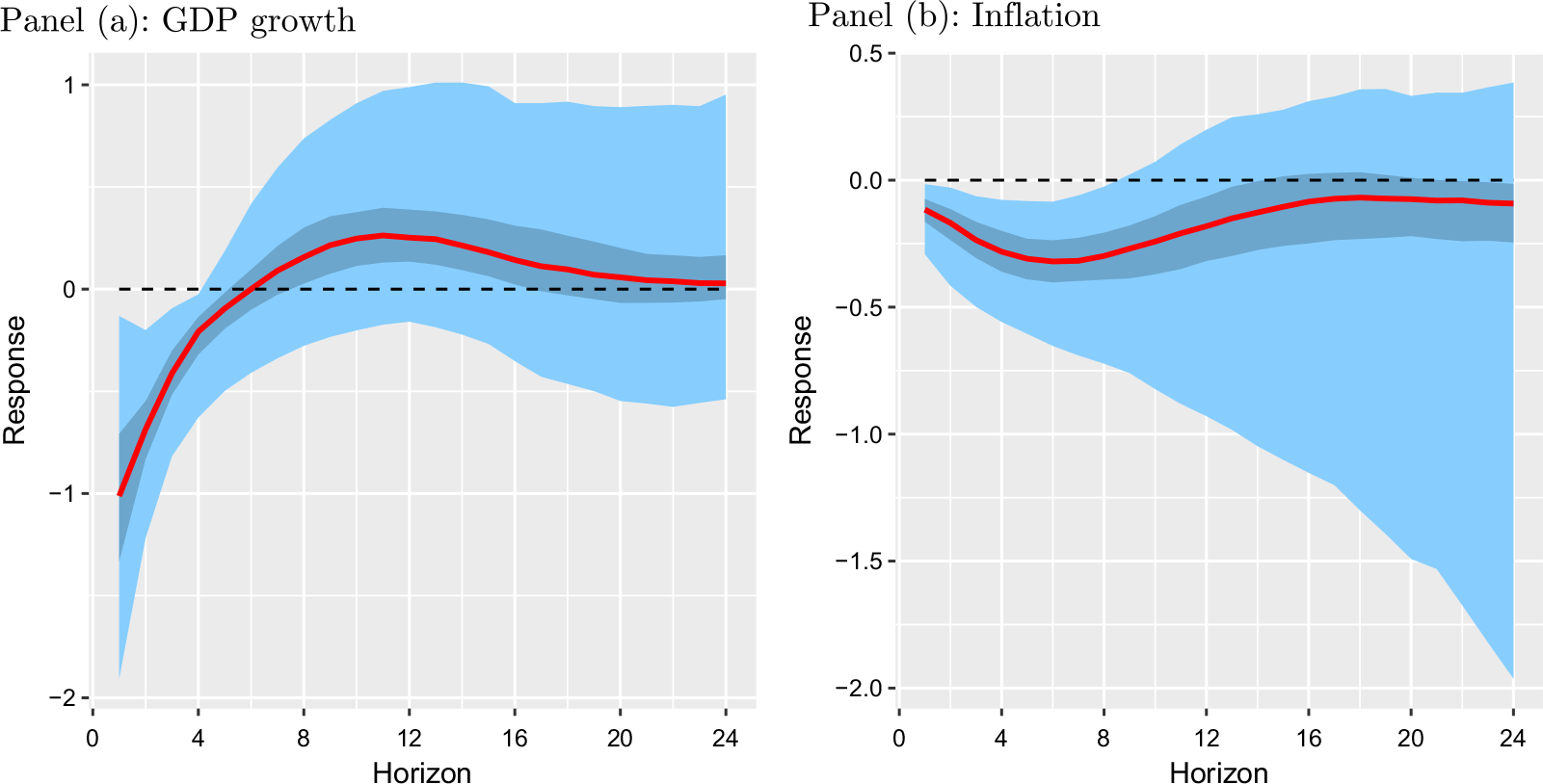
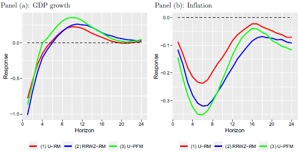
Figure 11 illustrates the reactions of real GDP growth and inflation to the considered monetary policy communication shock. As can be seen, hawkishness seems to result in a significant contraction of real GDP growth over a horizon of around a year (i.e., four quarters) and also a significant reduction in inflation, which holds for a horizon of roughly two years. We observe that the strongest impact on real GDP growth already materializes in the first quarter following the shock, while a severe reduction in prices shows up 1.5 years later. This analysis displays that the communication by the ECB also affects the real economy and especially the variable at the end of the monetary policy transmission process—actual consumer price inflation. The findings achieved in Figure 11 are not sensitive to variations in the algorithm used to obtain impulse responses. Figure 12 compares the responses resulting from the rejection method algorithm proposed by Rubio-Ramírez et al. (Reference Rubio-Ramírez, Waggoner and Zha2010) with the rejection method and the penalty function method suggested by Uhlig (Reference Uhlig2005) and basically confirms the findings.
Impulse response of a monetary policy communication shock.
Note: Panel (a) shows the reaction of real GDP growth to a monetary policy communication shock identified by sign restrictions using the rejection method algorithm proposed by Rubio-Ramírez et al. (Reference Rubio-Ramírez, Waggoner and Zha2010) based on a four variable SVAR with two lags including real GDP growth, inflation, the policy rate, and the aggregated sentiment measure derived from ECB press conferences. Panel (b) shows the corresponding reaction of inflation to the same shock. The red line gives the median reaction. The light (dark) blue shadings provide 95% (68%) confidence bands. Zero is indicated by a dashed line.
Robustness of the impulse response of a monetary policy communication shock.
Note: Panel (a) shows the reaction of real GDP growth to a monetary policy communication shock identified by sign restrictions based on a four variable SVAR with two lags including real GDP growth, inflation, the policy rate, and the aggregated sentiment measure derived from ECB press conferences using the rejection method algorithm proposed by Uhlig (Reference Uhlig2005) denoted as (1) U-RM and visualized by the red line, the rejection method algorithm suggested by Rubio-Ramírez et al. (Reference Rubio-Ramírez, Waggoner and Zha2010) denoted as (2) RRWZ-RM and visualized by the blue line, and the penalty function method algorithm proposed by Uhlig (Reference Uhlig2005) denoted as (3) U-PFM and visualized by the green line. Zero is indicated by a dashed line. Panel (b) shows the corresponding reaction of inflation to the same shock.
5. Conclusion
This study contributes to the existing literature by investigating the efficacy of ECB communication and its ability to predict several key variables. We employ text analysis tools to extract various sentiment measures from ECB press conferences, which signify either a dovish or hawkish tone. Subsequently, we assess the predictability of these sentiments on daily money market interest rates, while controlling for the ECB’s policy rate to determine whether policy communication provides additional information beyond actual interest rate changes. We also explore how central bank communication impacts inflation expectations and the associated dispersion and uncertainty about future inflation based on survey data. In addition, we explore whether the ECB’s communication strategy helps mitigate uncertainty related to monetary policy. Finally, we examine whether a policy communication shock, derived from the constructed sentiment and identified through sign restrictions, has the ability to affect real outcomes such as actual GDP growth and inflation. Our work differs from related studies that also propose similar measures of central bank communication sentiment. Picault and Renault (Reference Picault and Renault2017) assess whether the central bank communication conducted by the ECB can explain its future monetary decisions while considering an augmented Taylor rule. Máté et al. (Reference Máté, Sebők and Barczikay2021) study whether Hungarian central bank communication also affects Hungarian sovereign bond yields at different maturities. Our study focuses mainly on the effect of central bank communication on the interbank market and inflation expectations and therefore on the mechanism of transmission of monetary policy to the variables in between the two parts studied by Picault and Renault (Reference Picault and Renault2017) and Máté et al. (Reference Máté, Sebők and Barczikay2021).
Our key findings can be summarized as follows. First, we present compelling evidence demonstrating the predictability of interbank interest rates based on our constructed central bank communication sentiments documenting that the ECB’s communication policies and their tone have a role in influencing the monetary transmission process. Second, we observe that our inflation sentiment indicator exhibits predictive power when it comes to professional forecasters’ inflation expectations, the level of disagreement among them, and their uncertainty regarding future inflation. This suggests that the tone of the central bank’s communication is a factor that professionals take into account when shaping their expectations about future inflation. However, the ECB’s communication policies tend to contribute to a de-anchoring of inflation expectations, as they seem to have a positive effect on inflation expectations, disagreement, and uncertainty. Third, we also note significantly positive effects of our interest rate sentiment on the level of disagreement, volatility, and uncertainty concerning future policy rates. Finally, we demonstrate that policy communication shocks, identified through an SVAR with sign restrictions, also exert significant effects on the real economy. These findings enrich the existing literature and offer valuable insights for policymakers. In general, our results verify the significance of the tone of central bank communication throughout the various stages of the monetary policy transmission mechanism and demonstrate the usefulness of text analysis techniques in this context. However, they also suggest the need for refinements in the communication strategies and policies implemented by the ECB as our results indicate that the communication of the ECB hardly contributes to expectation anchoring and uncertainty reduction. Therefore, more research is required to shed further light on the effectiveness of central bank communication and how it can be best implemented. Another potential avenue for future research would be to study the impact of central bank communication on forecast revisions of professional forecasters to examine its role in forming expectations by market participants.
Acknowledgments
Thanks for valuable comments are due to two anonymous reviewers and the participants of the 8th International Workshop on Financial Markets and Nonlinear Dynamics (FMND) in Paris.
Appendix
Appendix A. Set of Keywords
List of keywords and adjectives for categorizing dovishness and hawkishness
An example of ECB monetary policy decision and ECB press conference
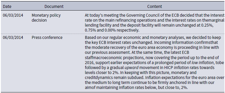
Appendix B. Descriptive Statistics of the Sentiments
Descriptive statistics of the four sentiments
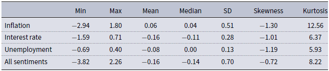
Correlation between the four sentiments
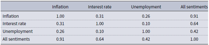
Accuracy measurement of in-sample forecast errors
Note: The table reports some forecast error statistics for the following regression:
 \begin{equation*} EONIA_t = \beta _0 + \beta _1 X_{t-k} + \beta _2 MRO_t + \epsilon _t, \end{equation*}
where $EONIA_t$
denotes the interbank interest rate,
$EONIA_t$
denotes the interbank interest rate, $X_{t-k}$
is the constructed sentiment measured from ECB press conferences for different lags
$X_{t-k}$
is the constructed sentiment measured from ECB press conferences for different lags $k=1,\ldots, 12$
, and
$k=1,\ldots, 12$
, and $MRO_t$
stands for the policy rate of the ECB (main refinancing operations rate). The forecast error statistics include the root mean squared error (RMSE), the mean absolute error (MAE), and the mean absolute percentage error (MAPE).
$MRO_t$
stands for the policy rate of the ECB (main refinancing operations rate). The forecast error statistics include the root mean squared error (RMSE), the mean absolute error (MAE), and the mean absolute percentage error (MAPE).
Appendix C. Robustness Checks
Interest rate pass-through coefficient of the policy rate (DFR).
Note: The plot shows the estimated $\beta _2$
coefficient of the following regression:
$\beta _2$
coefficient of the following regression:
 \begin{equation*} EONIA_t = \beta _0 + \beta _1 X_{t-k} + \beta _2 DFR_t + \epsilon _t, \end{equation*}
where $EONIA_t$
denotes the interbank interest rate,
$EONIA_t$
denotes the interbank interest rate, $X_{t-k}$
is the constructed sentiment measure from ECB press conferences for different lags
$X_{t-k}$
is the constructed sentiment measure from ECB press conferences for different lags $k=0,1,\ldots, 12$
, and
$k=0,1,\ldots, 12$
, and $DFR_t$
stands for the policy rate of the ECB (deposit facility rate instead of main refinancing operations rate). The points provide coefficient estimates and the whiskers indicate heteroscedasticity-and-autocorrelation-consistent (HAC) standard errors multiplied with the 97.5% quantiles of the standard normal distribution.
$DFR_t$
stands for the policy rate of the ECB (deposit facility rate instead of main refinancing operations rate). The points provide coefficient estimates and the whiskers indicate heteroscedasticity-and-autocorrelation-consistent (HAC) standard errors multiplied with the 97.5% quantiles of the standard normal distribution.
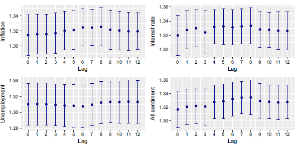
Effect of sentiment based on keywords on interbank interest rates.
Note: The plot shows the estimated $\beta _1$
coefficient of the following regression:
$\beta _1$
coefficient of the following regression:
 \begin{equation*} EONIA_t = \beta _0 + \beta _1 X_{t-k} + \beta _2 DFR_t + \epsilon _t, \end{equation*}
where $EONIA_t$
denotes the interbank interest rate,
$EONIA_t$
denotes the interbank interest rate, $X_{t-k}$
is the constructed sentiment measure from ECB press conferences for different lags
$X_{t-k}$
is the constructed sentiment measure from ECB press conferences for different lags $k=0,1,\ldots, 12$
, and
$k=0,1,\ldots, 12$
, and $DFR_t$
stands for the policy rate of the ECB (deposit facility rate instead of main refinancing operations rate). The points provide coefficient estimates and the whiskers indicate heteroscedasticity-and-autocorrelation-consistent (HAC) standard errors multiplied with the 97.5% quantiles of the standard normal distribution. The dashed black line is the zero line. The adjusted
$DFR_t$
stands for the policy rate of the ECB (deposit facility rate instead of main refinancing operations rate). The points provide coefficient estimates and the whiskers indicate heteroscedasticity-and-autocorrelation-consistent (HAC) standard errors multiplied with the 97.5% quantiles of the standard normal distribution. The dashed black line is the zero line. The adjusted $R^2$
in all regressions lies between 0.972 and 0.975.
$R^2$
in all regressions lies between 0.972 and 0.975.

Effect of inflation sentiment on inflation expectation.
Note: The plot shows the estimated $\beta _1$
coefficient of the following regression:
$\beta _1$
coefficient of the following regression:
 \begin{equation*} Y_{t,h} = \beta _0 + \beta _1 X_{t-k} + \beta _2 MRO_{t}+ \beta _3 EPU_{t} + \epsilon _t, \end{equation*}
where $Y_{t,h}$
denotes mean inflation expectations across professionals, the disagreement among professionals (i.e., the cross-sectional standard deviation across forecasters), the mean forecasters’ uncertainty regarding future inflation (i.e., the cross-sectional mean of the individual standard deviations of the density forecasts), or the mean kurtosis of the density forecasts across three different horizons (i.e., one-, two-, and five-years-ahead given by
$Y_{t,h}$
denotes mean inflation expectations across professionals, the disagreement among professionals (i.e., the cross-sectional standard deviation across forecasters), the mean forecasters’ uncertainty regarding future inflation (i.e., the cross-sectional mean of the individual standard deviations of the density forecasts), or the mean kurtosis of the density forecasts across three different horizons (i.e., one-, two-, and five-years-ahead given by $h=1,2,5$
).
$h=1,2,5$
). $X_{t-k}$
is the constructed inflation sentiment measure from ECB press conferences for different lags
$X_{t-k}$
is the constructed inflation sentiment measure from ECB press conferences for different lags $k=0,1,\ldots, 12$
and
$k=0,1,\ldots, 12$
and $EPU_t$
represents the economic policy uncertainty index for Europe following Baker et al. (Reference Baker, Bloom and Davis2016). The points provide coefficient estimates and the whiskers indicate heteroscedasticity-and-autocorrelation-consistent (HAC) standard errors multiplied with the 97.5% quantiles of the standard normal distribution. The dashed black line is the zero line. The red line represents the adjusted
$EPU_t$
represents the economic policy uncertainty index for Europe following Baker et al. (Reference Baker, Bloom and Davis2016). The points provide coefficient estimates and the whiskers indicate heteroscedasticity-and-autocorrelation-consistent (HAC) standard errors multiplied with the 97.5% quantiles of the standard normal distribution. The dashed black line is the zero line. The red line represents the adjusted $R^2$
.
$R^2$
.
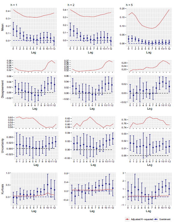
Effect of interest rate sentiment on inflation expectation.
Note: The plot shows the estimated $\beta _1$
coefficient of the following regression:
$\beta _1$
coefficient of the following regression:
 \begin{equation*} Y_{t,h} = \beta _0 + \beta _1 X_{t-k} + \beta _2 MRO_{t}+ \beta _3 EPU_{t} + \epsilon _t, \end{equation*}
where $Y_{t,h}$
denotes mean inflation expectations across professionals, the disagreement among professionals (i.e., the cross-sectional standard deviation across forecasters), the mean forecasters’ uncertainty regarding future inflation (i.e., the cross-sectional mean of the individual standard deviations of the density forecasts), or the mean kurtosis of the density forecasts across three different horizons (i.e., one-, two-, and five-years-ahead given by
$Y_{t,h}$
denotes mean inflation expectations across professionals, the disagreement among professionals (i.e., the cross-sectional standard deviation across forecasters), the mean forecasters’ uncertainty regarding future inflation (i.e., the cross-sectional mean of the individual standard deviations of the density forecasts), or the mean kurtosis of the density forecasts across three different horizons (i.e., one-, two-, and five-years-ahead given by $h=1,2,5$
).
$h=1,2,5$
). $X_{t-k}$
is the constructed interest rate sentiment measure from ECB press conferences for different lags
$X_{t-k}$
is the constructed interest rate sentiment measure from ECB press conferences for different lags $k=0,1,\ldots, 12$
and
$k=0,1,\ldots, 12$
and $EPU_t$
represents the economic policy uncertainty index for Europe following Baker et al. (Reference Baker, Bloom and Davis2016). The points provide coefficient estimates and the whiskers indicate heteroscedasticity-and-autocorrelation-consistent (HAC) standard errors multiplied with the 97.5% quantiles of the standard normal distribution. The dashed black line is the zero line. The red line represents the adjusted
$EPU_t$
represents the economic policy uncertainty index for Europe following Baker et al. (Reference Baker, Bloom and Davis2016). The points provide coefficient estimates and the whiskers indicate heteroscedasticity-and-autocorrelation-consistent (HAC) standard errors multiplied with the 97.5% quantiles of the standard normal distribution. The dashed black line is the zero line. The red line represents the adjusted $R^2$
.
$R^2$
.
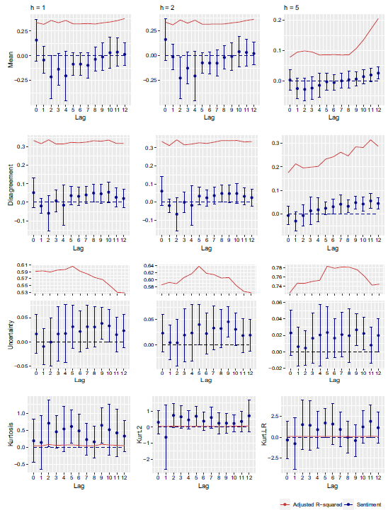
Appendix D. Shock Identification through Sign Restrictions
The adoption of sign restrictions is based on the idea of exploring the space of orthogonal shock decompositions to find reactions in line with the imposed restrictions. We adopt the following sign restrictions:
The algorithm is as follows:
-
1. We estimate the coefficients $\hat {B}_i$
for
$i=0,1,\ldots, p$
and the covariance matrix of the innovations
$\hat {\Sigma }$
of an unrestricted VARwhere
\begin{equation*} Z_{t}=B_0+\sum _{i=1}^pB_iZ_{t-i}+\nu _{t}, \end{equation*}
$Z_{t}=\{\text {GDP growth}_t,\pi _t,MRO_t,\text {Sentiment}_t\}$
.
$\hat {B}_i$
for
$i=0,1,\ldots, p$
and the covariance matrix of the innovations
$\hat {\Sigma }$
of an unrestricted VARwhere
\begin{equation*} Z_{t}=B_0+\sum _{i=1}^pB_iZ_{t-i}+\nu _{t}, \end{equation*}
$Z_{t}=\{\text {GDP growth}_t,\pi _t,MRO_t,\text {Sentiment}_t\}$
.
-
2. We apply a Cholesky decomposition to extract orthogonalized shocks from the estimated VAR model.
-
3. We compute the corresponding orthogonalized impulse responses for the shocks from Step 2.
-
4. We randomly draw an orthogonal impulse vector
$\alpha$
while
$\alpha =\tilde {A}a$
and
$\tilde {A}\tilde {A}^{\prime }=\tilde {\Sigma }$
. See Uhlig (Reference Uhlig2005) and Rubio-Ramírez et al. (Reference Rubio-Ramírez, Waggoner and Zha2010) for details. -
5. The responses from Step 3 are multiplied with the impulse vector
$\alpha$
from Step 4. Then, we check if these responses match the imposed sign restrictions. -
6. If yes, we keep the response. If not, we drop the draw.
-
7. We repeat Steps 2 to 6 until reaching 1,000 accepted draws.


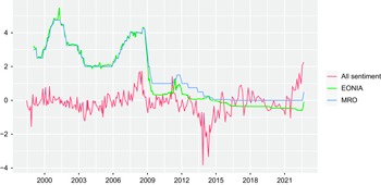


 Open access