





Impact statement
This work performs a biglobal input–output analysis of a canonical separated flow over a periodic hill. Results provide insights into the flow sensitivity, identifying the region and spatiotemporal scales where the external disturbance will be most effective in manipulating the flow response. Our input–output analysis also identifies the corresponding flow response and input–output amplification under the most sensitive disturbance. These insights can inform the flow sensitivity, receptivity, transition to turbulence and flow control of separated flows in engineering and geophysical applications, such as the flow over mountainous terrain, flow over an aerofoil and flow over blade tips in a turbine. Moreover, our biglobal input–output analysis employs the tensor product to directly construct differentiation matrices and associated spatiotemporal frequency response operator over a tensor product grid, which allows more flexibility to generalise this framework to a wider class of separated flows over complex geometries.
1. Introduction
Fluid flow over complex and curved structures is a very common scenario in engineering problems and in nature. These physical problems manifest themselves in real-world applications, such as in turbomachinery, aerospace engineering and geophysical applications (Almeida et al. Reference Almeida, Durao and Heitor1993). Some of these examples include flow over guiding vanes or blade tips in a turbine (Wheeler & Sandberg Reference Wheeler and Sandberg2016), flow over an aerofoil (Rolandi et al. Reference Rolandi, Smith, Amitay, Theofilis and Taira2025) or more naturally occurring flow over mountains (Belcher & Hunt Reference Belcher and Hunt1998). An important feature of these flows is the flow separation, which can be characterised by wall-layer thickening and recirculation with an increase in the wall-normal velocity field. Flow over a periodic hill is a canonical benchmark for understanding separated flows (Almeida et al. Reference Almeida, Durao and Heitor1993; Breuer et al. Reference Breuer, Peller, Rapp and Manhart2009; Günther & Von Rohr Reference Günther and Von Rohr2003; Li et al. Reference Li, Zhou, Yang, He and Chen2025; Rapp & Manhart Reference Rapp and Manhart2011; Xiao et al. Reference Xiao, Wu, Laizet and Duan2020; Zhou et al. Reference Zhou, Yang, Zhang and Yang2023), and it has been experimentally and numerically studied extensively. For example, Almeida et al. (Reference Almeida, Durao and Heitor1993) studied and measured mean and fluctuating flow over a periodic hill in both streamwise and spanwise directions. Various numerical and experimental studies were conducted to investigate flow separation, recirculation and reattachment (Breuer et al. Reference Breuer, Peller, Rapp and Manhart2009; Günther & Von Rohr Reference Günther and Von Rohr2003; Rapp & Manhart Reference Rapp and Manhart2011). Direct numerical simulations (DNS) of a series of flows over periodic hills were also compiled as a database for data-driven turbulence modelling (Xiao et al. Reference Xiao, Wu, Laizet and Duan2020).
Understanding and predicting flow separation over complex structures can be a difficult process because flow separation over curved surfaces is sensitive to various factors, such as incoming flow disturbance, the geometry of the structure, streamwise pressure gradient and interaction with the outer flow regime (Breuer et al. Reference Breuer, Peller, Rapp and Manhart2009; Rapp & Manhart Reference Rapp and Manhart2011). Another example of sensitivity to disturbances in separated flow is provided by Rolandi et al. (Reference Rolandi, Smith, Amitay, Theofilis and Taira2025), where the transition from wake-dominated structures to shear-dominated structures is observed as the disturbance frequency increases. Here, shear-dominated structures are flow structures with shorter length scales, which are more energetic and localised near the separation point and typically have higher temporal frequencies close to the characteristic frequency of a free shear layer (Ho and Huerre Reference Ho and Huerre1984; Kotapati et al. Reference Kotapati, Mittal, Marxen, Ham, You and Cattafesta2010; Rolandi et al. Reference Rolandi, Smith, Amitay, Theofilis and Taira2025). This shear-dominated dynamics is in contrast to that of global wake-dominated structures, which are less oscillatory and more coherent in space, seen at lower temporal frequencies of disturbances.
Uncovering the dominant flow structures that are generated and evolved by separated flow is important for solving the real-world problems we mentioned above. Modal analysis or decomposition has been utilised to extract the dominant flow structures while reducing the model complexity of the flow (Kutz et al. Reference Kutz, Brunton, Brunton and Proctor2016; Schmid & Henningson Reference Schmid and Henningson2012; Taira et al. Reference Taira, Brunton, Dawson, Rowley, Colonius, McKeon, Schmidt, Gordeyev, Theofilis and Ukeiley2017; Theofilis Reference Theofilis2011). These techniques help in the modelling, analysis and control of the fluid-flow system, thereby helping in achieving model-based design of various systems (Bagheri et al. Reference Bagheri, Henningson, Hœpffner and Schmid2009; Brunton and Noack Reference Brunton and Noack2015; Jovanović Reference Jovanović2021; Luhar et al. Reference Luhar, Sharma and McKeon2015; Moarref & Jovanović Reference Moarref and Jovanović2012; Ran et al. Reference Ran, Zare and Jovanović2021; Rowley & Dawson Reference Rowley and Dawson2017). Modal analysis techniques can be classified into data-driven or operator-based approaches (Rolandi et al. Reference Rolandi, Ribeiro, Yeh and Taira2024; Taira et al. Reference Taira, Brunton, Dawson, Rowley, Colonius, McKeon, Schmidt, Gordeyev, Theofilis and Ukeiley2017, Reference Taira, Hemati, Brunton, Sun, Duraisamy, Bagheri, Dawson and Yeh2020). Data-driven methods, such as dynamic mode decomposition, have been used to find a lower-order subspace to capture the effects of wake behind a flexible membrane and a jet passing between two cylinders (Schmid Reference Schmid2010). Recently, information-theoretic machine learning has also been used for mode decomposition of separated flows over an aerofoil (Fukami & Araki Reference Fukami and Araki2026).
Physics- or operator-based modal analysis includes global linear stability analysis (Jouin et al. Reference Jouin, Robinet and Cherubini2024; Taira et al. Reference Taira, Hemati, Brunton, Sun, Duraisamy, Bagheri, Dawson and Yeh2020; Tatsumi & Yoshimura Reference Tatsumi and Yoshimura1990; Theofilis Reference Theofilis2011; Yu et al. Reference Yu, Teo and Khoo2016) and input–output or resolvent analysis (Bamieh & Dahleh Reference Bamieh and Dahleh2001; Farrell & Ioannou Reference Farrell and Ioannou1993; Jovanović & Bamieh Reference Jovanović and Bamieh2005; Jovanović Reference Jovanović2021; Liu & Gayme Reference Liu and Gayme2020, Reference Liu and Gayme2021; McKeon Reference McKeon2017). Both methods rely on the linearised Navier–Stokes equations and depend on the base flow obtained from DNS or experimental results for identifying the dominant flow structures. To conduct global linear stability analysis, we need to construct a linear operator from linearised Navier–Stokes equations and then perform an eigenvalue analysis of this linear operator to obtain the growth rate (Moradi & Floryan Reference Moradi and Floryan2014; Picella et al. Reference Picella, Loiseau, Lusseyran, Robinet, Cherubini and Pastur2018; Sun et al. Reference Sun, Taira, Cattafesta and Ukeiley2017; Szumbarski & Floryan Reference Szumbarski and Floryan2006; Theofilis Reference Theofilis2011; de Vicente et al. Reference de Vicente, Basley, Meseguer-Garrido, Soria and Theofilis2014). Input–output or resolvent analysis considers the linearised Navier–Stokes equation disturbed by an additional forcing term, which can represent free-stream disturbance, experimental uncertainty, background noise and model uncertainty. Such input forcing is then mapped to certain outputs of interest through a spatiotemporal frequency response operator or a resolvent operator. At every wavenumber–frequency combination, the singular value decomposition of the frequency response operator is performed (Jovanović, Reference Jovanović2021; McKeon Reference McKeon2017; Rolandi et al., Reference Rolandi, Ribeiro, Yeh and Taira2024), which uncovers the dominant or most amplified flow structures. Such singular value decomposition also identifies how minimal forcing can cause an exaggerated response at certain frequencies, which makes it an effective tool for guiding active flow control (Lin et al. Reference Lin, Tsai and Tsai2023; Liu et al. Reference Liu, Sun, Yeh, Ukeiley, Cattafesta and Taira2021; Yeh & Taira Reference Yeh and Taira2019).
Resolvent analysis has also been extended to analyse flow over complex geometry, such as riblets (Chavarin & Luhar Reference Chavarin and Luhar2020; Ran et al. Reference Ran, Zare and Jovanović2021; Naseri & Zare Reference Naseri and Zare2025), compliant walls (Luhar et al. Reference Luhar, Sharma and McKeon2015) and porous substrates (Chavarin et al. Reference Chavarin, Gomez-de Segura, Garcia-Mayoral and Luhar2021). For flow over riblets, resolvent analysis can help design and optimise the geometry of riblets, allowing us to understand the dynamics of secondary flow generated under various protrusion heights of the ribs (Chavarin & Luhar Reference Chavarin and Luhar2020). Furthermore, such resolvent analysis has been exploited to understand flow separation and reattachment at various frequencies of separated flow over an aerofoil (Houtman et al. Reference Houtman, Timme and Sharma2023; Ribeiro & Taira Reference Ribeiro and Taira2024; Rolandi et al. Reference Rolandi, Smith, Amitay, Theofilis and Taira2025; Thomareis & Papadakis Reference Thomareis and Papadakis2018; Yeh et al. Reference Yeh, Benton, Taira and Garmann2020). Moreover, resolvent analysis of cavity flow shows that forcing mode peaks near the leading edge of the cavity, while response mode peaks at certain downstream locations close to the trailing edge (Islam & Sun Reference Islam and Sun2024; Liu & Gaitonde Reference Liu and Gaitonde2021; Sun et al. Reference Sun, Liu, Cattafesta, Ukeiley and Taira2020). By understanding the least stabilising frequencies through resolvent analysis, increased aerodynamic loading can be achieved by laminar separation control (Gross et al. Reference Gross, Marks and Sondergaard2024). Understanding flow separation, recirculation and reattachment through input–output analysis can be extended to other separated flows or wake flows, such as flow over cylinders and other stationary or moving objects (Feng et al. Reference Feng, Gupta, Li and Wan2024; Jin et al. Reference Jin, Symon and Illingworth2021; Li & Yang Reference Li and Yang2024; Lin et al. Reference Lin, Tsai and Tsai2023).
Within resolvent analysis, a complex geometry is usually modelled as the volume penalty method (VPM) (Chavarin & Luhar Reference Chavarin and Luhar2020; Ran et al. Reference Ran, Zare and Jovanović2021). The VPM uses a Brinkman-type penalisation with varying permeability to model a solid system immersed within a fluid domain (Angot Reference Angot1999), in the same spirit as the immersed boundary method (Mittal & Iaccarino Reference Mittal and Iaccarino2005; Peskin Reference Peskin2002; Taira & Colonius Reference Taira and Colonius2007; Verzicco Reference Verzicco2023). These methods allow us to couple the fluid and the solid system in a single numerical domain (Angot Reference Angot1999), and thus avoid the body-fitting grid and coordinate transformation required in classical methods such as the arbitrary Lagrangian–Eulerian method (Diosady & Murman Reference Diosady and Murman2014). The VPM approximates the no-slip boundary condition by rapid linear damping (Hester et al. Reference Hester, Vasil and Burns2021) and can be extended to moving and deformable bodies (Engels et al. Reference Engels, Kolomenskiy, Schneider and Sesterhenn2015). Although some recent work implements the immersed boundary method within resolvent analysis (Flynn et al. Reference Flynn, Bae and Goza2024; Hou & Colonius Reference Hou and Colonius2023), the VPM has an advantage in that it does not require computing the penalty body force through interpolation, which is more suitable for resolvent or input–output analysis performed in the frequency domain (Chavarin & Luhar Reference Chavarin and Luhar2020; Ran et al. Reference Ran, Zare and Jovanović2021).
In this work, we conduct a biglobal input–output analysis of flow over a periodic hill to uncover the underlying dominant flow structures and to understand the flow sensitivity to disturbance. The streamwise periodicity of this flow allows us to isolate the flow separation from the spatially developing effects, and the smooth geometry of the periodic hill also allows us to avoid the Rossiter modes (Rossiter Reference Rossiter1964; Sun et al. Reference Sun, Taira, Cattafesta and Ukeiley2017) observed in flow over a rectangular cavity. We model the periodic hill using an improved VPM framework, where asymptotic analysis has been conducted to determine an optimal mask function that can lead to improved accuracy (Hester et al. Reference Hester, Vasil and Burns2021). This improved VPM approach has a faster convergence rate of the model error as the damping time scale approaches zero (Hester et al. Reference Hester, Vasil and Burns2021), compared with previous VPM frameworks (Angot Reference Angot1999; Carbou & Fabrie Reference Carbou and Fabrie2003). We utilise the same VPM model in both DNS and input–output analysis. We use DNS to generate the two-dimensional (2-D) base flows, which are then used to formulate the resolvent operator within biglobal input–output analysis. Here, biglobal is used in the same sense as in biglobal linear stability analysis (Theofilis Reference Theofilis2011), where our base flow depends on two spatial coordinates: streamwise and wall-normal directions. Similar biglobal resolvent or input–output analysis has been widely employed to 2-D base flow induced by streamwise-travelling waves (Moarref & Jovanović Reference Moarref and Jovanović2010), flow over riblets (Chavarin & Luhar Reference Chavarin and Luhar2020; Ran et al. Reference Ran, Zare and Jovanović2021) and separated flow over an aerofoil (Ribeiro & Taira Reference Ribeiro and Taira2024; Rolandi et al. Reference Rolandi, Smith, Amitay, Theofilis and Taira2025; Yeh & Taira Reference Yeh and Taira2019; Yeh et al. Reference Yeh, Benton, Taira and Garmann2020). This work not only applies biglobal input–output analysis to flow over periodic hills, but also directly utilises the tensor product (i.e. Kronecker product) to form differentiation matrices on a tensor product grid (Trefethen Reference Trefethen2000). This tensor product approach avoids the Fourier transform of the base flow and the penalty force modelling the solid body (Chavarin & Luhar, Reference Chavarin and Luhar2020; Ran et al., Reference Ran, Zare and Jovanović2021), and thus, this approach allows a more straightforward manner to formulate and implement the resolvent operator associated with 2-D base flows. We analyse the forcing and response modes of flow over a periodic hill at various spatiotemporal frequencies and Reynolds numbers to understand the effect of external disturbance on the flow response.
The rest of the paper is organised as follows. We set up our problem of flow over a periodic hill and modelling approach using the VPM in § 2. Section 3 then presents DNS to obtain base flows and validate our VPM. In § 4, we discuss the formulation of the biglobal input–output analysis and present results. We conclude this paper and discuss future directions in § 5.
2. Problem set-up and modelling based on volume penalty method
2.1. Flow over periodic hill
We consider incompressible flow over an idealised periodic hill defined in Cartesian coordinates along the streamwise $(x)$
, wall-normal
$(x)$
, wall-normal $(y)$
and spanwise
$(y)$
and spanwise $(z)$
directions (figure 1
a). The velocity vector is denoted as
$(z)$
directions (figure 1
a). The velocity vector is denoted as $\mathbf{u} = [u,v,w]^{\text{T}}$
, where
$\mathbf{u} = [u,v,w]^{\text{T}}$
, where $u$
,
$u$
, $v$
and
$v$
and $w$
are velocity components in streamwise, wall-normal and spanwise directions, respectively. Here, the superscript
$w$
are velocity components in streamwise, wall-normal and spanwise directions, respectively. Here, the superscript $^{\text{T}}$
denotes the transpose, and
$^{\text{T}}$
denotes the transpose, and $p$
denotes the pressure. The dynamics of fluid flow is governed by the incompressible Navier–Stokes equations:
$p$
denotes the pressure. The dynamics of fluid flow is governed by the incompressible Navier–Stokes equations:
 \begin{align} \frac {\partial \mathbf{u}}{\partial t} + \mathbf{u}\cdot \nabla \mathbf{u} & = -\nabla p + \frac {1}{{Re}} \nabla ^{2}\mathbf{u} + \mathbf{F}+ \mathbf{f}, \quad \quad \nabla \cdot \mathbf{u} = 0. \end{align}
Here, $\mathbf{F}$
is a linear damping penalty term to model the solid domain and
$\mathbf{F}$
is a linear damping penalty term to model the solid domain and $\mathbf{f}$
is the input forcing term that will be used in input–output analysis in § 4, which can represent the free-stream disturbance, experimental uncertainty, background noise and model uncertainty. Here, the length is normalised by the maximal height of the periodic hill
$\mathbf{f}$
is the input forcing term that will be used in input–output analysis in § 4, which can represent the free-stream disturbance, experimental uncertainty, background noise and model uncertainty. Here, the length is normalised by the maximal height of the periodic hill $H$
and the velocity is normalised by the bulk velocity
$H$
and the velocity is normalised by the bulk velocity $U_b^*$
, which leads to the Reynolds number defined as
$U_b^*$
, which leads to the Reynolds number defined as $Re= {U_b^* H}/{\nu }$
with
$Re= {U_b^* H}/{\nu }$
with $\nu$
as the kinematic viscosity.
$\nu$
as the kinematic viscosity.
We consider a periodic hill geometry with non-dimensional height (Fischer et al. Reference Fischer, Lottes and Tufo2007) as $y_{\text{hill}}(x)=3C [1 + \tanh (B(\lvert x - A\rvert - B))],$
where
$y_{\text{hill}}(x)=3C [1 + \tanh (B(\lvert x - A\rvert - B))],$
where $A = 4.5$
,
$A = 4.5$
, $B = 3.5$
and
$B = 3.5$
and $C = 1/6$
. The hill has a width along the streamwise direction at its base that is two times the maximal height of the hill. We consider a wall-normal domain as
$C = 1/6$
. The hill has a width along the streamwise direction at its base that is two times the maximal height of the hill. We consider a wall-normal domain as $y\in [0,3]$
and a streamwise domain as
$y\in [0,3]$
and a streamwise domain as $x\in [0,9]$
. We choose such periodic hill geometry and computation domain to be consistent with the problem set-up of the flow over the periodic hill example in Nek5000 software (Fischer et al. Reference Fischer, Lottes and Tufo2007). This helps us with validating our results against Nek5000, described later in § 3.
$x\in [0,9]$
. We choose such periodic hill geometry and computation domain to be consistent with the problem set-up of the flow over the periodic hill example in Nek5000 software (Fischer et al. Reference Fischer, Lottes and Tufo2007). This helps us with validating our results against Nek5000, described later in § 3.
(a) Illustration of periodic hill geometry with $L_x, L_y, L_z$
as the domain size in streamwise, wall-normal and spanwise directions. (b) The value of the mask function
$L_x, L_y, L_z$
as the domain size in streamwise, wall-normal and spanwise directions. (b) The value of the mask function $\Gamma$
with
$\Gamma$
with ${\Gamma }\rightarrow 1$
in the solid domain,
${\Gamma }\rightarrow 1$
in the solid domain, ${\Gamma }\rightarrow 0$
in the fluid region and a smooth transition through the solid–fluid interface.
${\Gamma }\rightarrow 0$
in the fluid region and a smooth transition through the solid–fluid interface.

Figure 1 Long description
The diagram consists of two parts. The left part shows a three-dimensional domain for fluid flow over a periodic hill, with dimensions labeled as Lx, Ly, and Lz in the streamwise, wall-normal, and spanwise directions respectively. The axes are labeled x, y, z with corresponding velocity components u, v, w. The right part depicts a two-dimensional cross-section of the domain, highlighting the mask function values. The mask function is represented with a gradient scale from 0 to 1, indicating the transition from the solid domain to the fluid region. The solid domain is labeled as Ωs, the fluid region as Ωf, and the boundary as ∂Ω. The flow direction is indicated by an arrow pointing to the right.
2.2. Volume penalty method
Here, we employ an improved VPM (Hester et al. Reference Hester, Vasil and Burns2021) to model the solid domain of a periodic hill. This VPM allows us to employ the same modelling approach for both DNS and input–output analysis (Chavarin & Luhar Reference Chavarin and Luhar2020; Ran et al. Reference Ran, Zare and Jovanović2021). The domain $\Omega$
is partitioned into
$\Omega$
is partitioned into $\Omega _f$
for the fluid part and
$\Omega _f$
for the fluid part and $\Omega _s$
for the solid part of the domain, as shown in figure 1(b). The fluid–solid interface is given as
$\Omega _s$
for the solid part of the domain, as shown in figure 1(b). The fluid–solid interface is given as $\partial \Omega$
, and the VPM aims to impose no-slip and no-penetration boundary conditions at this interface, i.e.
$\partial \Omega$
, and the VPM aims to impose no-slip and no-penetration boundary conditions at this interface, i.e. $\mathbf{u}|_{\partial \Omega } = \mathbf{0}$
.
$\mathbf{u}|_{\partial \Omega } = \mathbf{0}$
.
We employ the penalty forcing term $\mathbf{F}$
in the momentum equation in (2.1) as a linear damping term:
$\mathbf{F}$
in the momentum equation in (2.1) as a linear damping term:
 \begin{equation} \mathbf{F} = - \frac {\Gamma }{\eta } (\mathbf{u} - \mathbf{u}_{\text{solid}}), \end{equation}
where $\mathbf{u}_{\text{solid}}=\mathbf{0}$
as we consider a stationary periodic hill. In (2.2),
$\mathbf{u}_{\text{solid}}=\mathbf{0}$
as we consider a stationary periodic hill. In (2.2), $\Gamma$
is the normalised mask function and
$\Gamma$
is the normalised mask function and $\eta$
is the non-dimensional damping time scale. The mask function
$\eta$
is the non-dimensional damping time scale. The mask function $\Gamma :\Omega \rightarrow [0,1]$
is employed to locate the solid object and the interface in the domain (Hester et al. Reference Hester, Vasil and Burns2021), where
$\Gamma :\Omega \rightarrow [0,1]$
is employed to locate the solid object and the interface in the domain (Hester et al. Reference Hester, Vasil and Burns2021), where $\Gamma =1$
in the solid domain and
$\Gamma =1$
in the solid domain and $\Gamma =0$
in the fluid domain with a smooth transition at the solid–fluid interface. Here, we generate the mask function by selecting a normalised mask function
$\Gamma =0$
in the fluid domain with a smooth transition at the solid–fluid interface. Here, we generate the mask function by selecting a normalised mask function $\hat {\Gamma }$
, which has to satisfy certain important properties (Hester et al. Reference Hester, Vasil and Burns2021): (i) boundedness:
$\hat {\Gamma }$
, which has to satisfy certain important properties (Hester et al. Reference Hester, Vasil and Burns2021): (i) boundedness: $\hat {\Gamma }:\mathbb{R}\rightarrow [0,1]$
; (ii) smoothness: at least
$\hat {\Gamma }:\mathbb{R}\rightarrow [0,1]$
; (ii) smoothness: at least $C^1$
continuous; (iii) limiting behaviour:
$C^1$
continuous; (iii) limiting behaviour: $\lim _{x\to -\infty }\hat {\Gamma }(x)=1$
and
$\lim _{x\to -\infty }\hat {\Gamma }(x)=1$
and $\lim _{x\to \infty }\hat {\Gamma }(x)=0$
; (iv) monotonicity:
$\lim _{x\to \infty }\hat {\Gamma }(x)=0$
; (iv) monotonicity: $x_2 \gt x_1 \Rightarrow \hat {\Gamma }(x_2) \lt \Gamma (x_1)$
; and (v) symmetry:
$x_2 \gt x_1 \Rightarrow \hat {\Gamma }(x_2) \lt \Gamma (x_1)$
; and (v) symmetry: $\hat {\Gamma }(x) + \hat {\Gamma }(-x) = 1$
. We choose an error function as the normalised mask function
$\hat {\Gamma }(x) + \hat {\Gamma }(-x) = 1$
. We choose an error function as the normalised mask function $\hat {\Gamma }_{\text{erf}}$
to satisfy the conditions we listed (Hester et al. Reference Hester, Vasil and Burns2021):
$\hat {\Gamma }_{\text{erf}}$
to satisfy the conditions we listed (Hester et al. Reference Hester, Vasil and Burns2021):
 \begin{equation} \hat {\Gamma }_{\mathrm{erf}}(d_{\perp }) = \tfrac {1}{2}(1 - \operatorname {erf}(\!\sqrt {\pi }\,d_{\perp })), \end{equation}
where $\text{erf}(x)$
is the error function
$\text{erf}(x)$
is the error function $\mathrm{erf}(x) = ({2}/{\sqrt {\pi }}) \int _{0}^{x} {\rm e}^{-t^{2}}\, \text{d}t$
. In (2.3),
$\mathrm{erf}(x) = ({2}/{\sqrt {\pi }}) \int _{0}^{x} {\rm e}^{-t^{2}}\, \text{d}t$
. In (2.3), $d_{\perp }$
is the signed distance from the boundary of the periodic hill, which is defined as the distance of any point on the grid to the closest point
$d_{\perp }$
is the signed distance from the boundary of the periodic hill, which is defined as the distance of any point on the grid to the closest point $p$
on the interface
$p$
on the interface $\partial \Omega$
. We have
$\partial \Omega$
. We have $d_{\perp }\gt 0$
for the fluid domain,
$d_{\perp }\gt 0$
for the fluid domain, $d_{\perp }\lt 0$
for the solid domain and
$d_{\perp }\lt 0$
for the solid domain and $d_{\perp }=0$
at the solid–fluid interface. Then, we can construct our mask function using
$d_{\perp }=0$
at the solid–fluid interface. Then, we can construct our mask function using $\hat {\Gamma }_{\text{erf}}$
as
$\hat {\Gamma }_{\text{erf}}$
as
 \begin{equation} \Gamma (d_{\perp }) = \hat {\Gamma }_{\mathrm{erf}}\left (\frac {d_{\perp }}{\delta ^*}\right ), \end{equation}
where $\delta ^{*}$
is the optimum thickness of the numerical interface.
$\delta ^{*}$
is the optimum thickness of the numerical interface.
We discuss how we choose $\eta$
in (2.2) and
$\eta$
in (2.2) and $\delta ^*$
in (2.4) used in the VPM following Hester et al. (Reference Hester, Vasil and Burns2021). Here, the non-dimensional damping time scale
$\delta ^*$
in (2.4) used in the VPM following Hester et al. (Reference Hester, Vasil and Burns2021). Here, the non-dimensional damping time scale $\eta$
is defined as
$\eta$
is defined as $\eta = \tau U_b^*/H$
, where
$\eta = \tau U_b^*/H$
, where $\tau$
is the dimensional damping time scale. We also introduce the non-dimensional damping length scale
$\tau$
is the dimensional damping time scale. We also introduce the non-dimensional damping length scale $\epsilon = \sqrt {\nu \tau }/H$
. Here,
$\epsilon = \sqrt {\nu \tau }/H$
. Here, $\eta$
measures the ratio of damping and inertial time scales, and
$\eta$
measures the ratio of damping and inertial time scales, and $\epsilon$
is the ratio of the viscous length and the damping length scale, which are related to each other by
$\epsilon$
is the ratio of the viscous length and the damping length scale, which are related to each other by $\eta =Re\epsilon ^2$
. The damping time scale
$\eta =Re\epsilon ^2$
. The damping time scale $\eta$
and length scale
$\eta$
and length scale $\epsilon$
have a strong correlation, and they are equal to each other when
$\epsilon$
have a strong correlation, and they are equal to each other when $\eta$
=
$\eta$
= $\epsilon$
=
$\epsilon$
= $ {1}/{Re}$
(Hester et al. Reference Hester, Vasil and Burns2021). Based on the relation between
$ {1}/{Re}$
(Hester et al. Reference Hester, Vasil and Burns2021). Based on the relation between $\eta$
and
$\eta$
and $\epsilon$
, either the damping time scale or the length scale dominates the other, leading to various model errors (Hester et al. Reference Hester, Vasil and Burns2021). When
$\epsilon$
, either the damping time scale or the length scale dominates the other, leading to various model errors (Hester et al. Reference Hester, Vasil and Burns2021). When $\epsilon \gt \eta$
, the damping is strongest, resulting in second-order convergence, while
$\epsilon \gt \eta$
, the damping is strongest, resulting in second-order convergence, while $\eta \gt \epsilon$
corresponds to intermediate damping. To reduce free parameters in the VPM, we select the
$\eta \gt \epsilon$
corresponds to intermediate damping. To reduce free parameters in the VPM, we select the $\eta =\epsilon = {1}/{Re}$
regime where the damping length scale and time scale are equal to each other, which is between the strong damping and the intermediate damping regimes (Hester et al. Reference Hester, Vasil and Burns2021). According to Hester et al. (Reference Hester, Vasil and Burns2021), we choose the optimal interface thickness
$\eta =\epsilon = {1}/{Re}$
regime where the damping length scale and time scale are equal to each other, which is between the strong damping and the intermediate damping regimes (Hester et al. Reference Hester, Vasil and Burns2021). According to Hester et al. (Reference Hester, Vasil and Burns2021), we choose the optimal interface thickness $\delta ^{*} = 3.1134 \epsilon$
, which leads to
$\delta ^{*} = 3.1134 \epsilon$
, which leads to $\mathcal{O}(\epsilon ^2)$
convergence in the strong damping regime as an improvement on previous VPM frameworks (Angot Reference Angot1999; Carbou and Fabrie Reference Carbou and Fabrie2003). The value of
$\mathcal{O}(\epsilon ^2)$
convergence in the strong damping regime as an improvement on previous VPM frameworks (Angot Reference Angot1999; Carbou and Fabrie Reference Carbou and Fabrie2003). The value of $\Gamma$
associated with this optimal interface thickness
$\Gamma$
associated with this optimal interface thickness $\delta ^*$
is shown in figure 1(b).
$\delta ^*$
is shown in figure 1(b).
3. Direct numerical simulation to obtain base flow
Here, we implement the VPM described in § 2.2 into the spectral solver Dedalus (Burns et al. Reference Burns, Vasil, Oishi, Lecoanet and Brown2020), and we refer to this implementation as Dedalus-VPM. We then use Dedalus-VPM to obtain the 2-D time-averaged base flow $\mathbf{U}=[U(x,y),V(x,y),0]^{\text{T}}$
that will be used for the input–output analysis in § 4. We impose periodic boundary conditions in the streamwise direction and impose Dirichlet boundary conditions for the velocity field at the bottom and top of the domain, i.e.
$\mathbf{U}=[U(x,y),V(x,y),0]^{\text{T}}$
that will be used for the input–output analysis in § 4. We impose periodic boundary conditions in the streamwise direction and impose Dirichlet boundary conditions for the velocity field at the bottom and top of the domain, i.e. $\mathbf{u}(x,\,y=0,\,t) =\mathbf{u}(x,\,y= L_y,\,t)= \mathbf{0}$
. We discretise (2.1) using the Fourier spectral method in the streamwise direction and the Chebyshev spectral method in the wall-normal direction. For simulation results in this section, the input forcing
$\mathbf{u}(x,\,y=0,\,t) =\mathbf{u}(x,\,y= L_y,\,t)= \mathbf{0}$
. We discretise (2.1) using the Fourier spectral method in the streamwise direction and the Chebyshev spectral method in the wall-normal direction. For simulation results in this section, the input forcing $\mathbf{f}$
in (2.1) is set to zero. As we normalise the velocity scale by the bulk velocity
$\mathbf{f}$
in (2.1) is set to zero. As we normalise the velocity scale by the bulk velocity $U_b^*$
, we have the non-dimensional bulk velocity as
$U_b^*$
, we have the non-dimensional bulk velocity as $U_b=1$
. This bulk velocity is imposed by setting the flow rate
$U_b=1$
. This bulk velocity is imposed by setting the flow rate $Q:=\int _{\Omega _f} u(x,y,z,t)\, \text{d}A$
as
$Q:=\int _{\Omega _f} u(x,y,z,t)\, \text{d}A$
as $Q= U_b |{\Omega _f}|$
in simulation, where
$Q= U_b |{\Omega _f}|$
in simulation, where $|{\Omega _f}|$
denotes the area of the fluid domain. Using bulk velocity as a constraint allows the pressure gradient to vary dynamically while ensuring that the simulation runs at the desired Reynolds number defined by the bulk velocity. The statistically steady state obtained from the DNS is then used to compute the time-averaged base flow
$|{\Omega _f}|$
denotes the area of the fluid domain. Using bulk velocity as a constraint allows the pressure gradient to vary dynamically while ensuring that the simulation runs at the desired Reynolds number defined by the bulk velocity. The statistically steady state obtained from the DNS is then used to compute the time-averaged base flow $\mathbf{U}$
.
$\mathbf{U}$
.
Steady-state flow (a) $U(x,y)$
and (b)
$U(x,y)$
and (b) $V(x,y)$
obtained from Dedalus-VPM at
$V(x,y)$
obtained from Dedalus-VPM at $Re = 100$
.
$Re = 100$
.

Figure 2 Long description
A heat map displays steady-state flow patterns in two different scenarios. The first subplot (a) shows a rectangular region with a color gradient ranging from light to dark red, indicating varying flow intensities. The x-axis ranges from 0 to 9, and the y-axis ranges from 0 to 3. The color scale on the right indicates values from -0.15 to 1.93. The second subplot (b) shows a similar rectangular region with contour lines representing flow patterns. The x-axis and y-axis have the same range as in subplot (a). The color scale on the right indicates values from -0.07 to 0.27. Both subplots highlight regions of high and low flow intensity, with distinct patterns and gradients visible.
Here, we examine the flow over a periodic hill at $Re = 100$
. We use a grid size of
$Re = 100$
. We use a grid size of $(N_x,N_y)=(352, 512)$
in
$(N_x,N_y)=(352, 512)$
in $x$
and
$x$
and $y$
directions, and the maximum non-dimensional time step is 0.005. At this Reynolds number, the flow remains laminar and will converge to a steady state after the initial transient. Figure 2 shows the steady-state streamwise velocity
$y$
directions, and the maximum non-dimensional time step is 0.005. At this Reynolds number, the flow remains laminar and will converge to a steady state after the initial transient. Figure 2 shows the steady-state streamwise velocity $U(x,y)$
and wall-normal velocity
$U(x,y)$
and wall-normal velocity $V(x,y)$
of flow over a periodic hill using Dedalus-VPM at
$V(x,y)$
of flow over a periodic hill using Dedalus-VPM at $Re = 100$
. The streamwise velocity in figure 2(a) shows shear-layer formation between low-speed recirculation regions (
$Re = 100$
. The streamwise velocity in figure 2(a) shows shear-layer formation between low-speed recirculation regions ( $y\lt 0.6$
) and the region above the hill (
$y\lt 0.6$
) and the region above the hill ( $y\gt 1$
) with a higher velocity. The wall-normal velocity
$y\gt 1$
) with a higher velocity. The wall-normal velocity $V(x,y)$
in figure 2(b) shows an upward motion near the hill crest
$V(x,y)$
in figure 2(b) shows an upward motion near the hill crest $(x\approx 8)$
and a downward motion near
$(x\approx 8)$
and a downward motion near $x\approx 4$
. We observe a large recirculation bubble downstream of the hill, and the recirculation bubble is stable at this Reynolds number. Flow separation occurs close to the top of the downstream side of the hill
$x\approx 4$
. We observe a large recirculation bubble downstream of the hill, and the recirculation bubble is stable at this Reynolds number. Flow separation occurs close to the top of the downstream side of the hill $(x \approx 1)$
, creating recirculation, and the flow gets quicker downstream as it approaches the hill crest at
$(x \approx 1)$
, creating recirculation, and the flow gets quicker downstream as it approaches the hill crest at $x=9$
.
$x=9$
.
Now we look at the unsteady case of $Re = 190$
, where the flow is found to be unsteady. According to Breuer et al. (Reference Breuer, Peller, Rapp and Manhart2009), flow at
$Re = 190$
, where the flow is found to be unsteady. According to Breuer et al. (Reference Breuer, Peller, Rapp and Manhart2009), flow at $Re = 200$
is unsteady and shows three-dimensional effects after the initial transient of 2-D flow. We select
$Re = 200$
is unsteady and shows three-dimensional effects after the initial transient of 2-D flow. We select $Re=190$
to be close to but lower than this
$Re=190$
to be close to but lower than this $Re=200$
value to minimise the impact of spanwise motion not included in our 2-D simulations. A grid of
$Re=200$
value to minimise the impact of spanwise motion not included in our 2-D simulations. A grid of $ (N_x,N_y)=(384, 576)$
has been chosen for the Dedalus-VPM model. From the time-averaged mean flow profile
$ (N_x,N_y)=(384, 576)$
has been chosen for the Dedalus-VPM model. From the time-averaged mean flow profile $U(x,y)$
in figure 3, we still observe the flow separation and reattachment downstream of the hill from the time-averaged velocity, although the recirculation bubble is unsteady.
$U(x,y)$
in figure 3, we still observe the flow separation and reattachment downstream of the hill from the time-averaged velocity, although the recirculation bubble is unsteady.
Time-averaged flow (a) $U(x,y)$
and (b)
$U(x,y)$
and (b) $V(x,y)$
obtained from Dedalus-VPM at
$V(x,y)$
obtained from Dedalus-VPM at $Re = 190$
.
$Re = 190$
.

Figure 3 Long description
The heat map consists of two subplots labeled (a) and (b), each representing different aspects of the time-averaged flow over a periodic hill. Subplot (a) displays a gradient of values ranging from -0.24 to 1.97, with darker reds indicating higher values and lighter areas indicating lower values. Subplot (b) shows a similar gradient ranging from -0.19 to 0.21. Both subplots feature contour lines that highlight regions of similar values, with noticeable recirculation patterns near the base of the hill. The x-axis ranges from 0 to 9, and the y-axis ranges from 0 to 3. The color intensity varies significantly, indicating areas of flow separation and recirculation.
3.1. Implementation of no-slip boundary conditions
Steady-state streamwise velocity $U(x,y)$
and
$U(x,y)$
and $y_{\text{hill}}(x)$
at three streamwise locations with
$y_{\text{hill}}(x)$
at three streamwise locations with $Re = 100$
: (a)
$Re = 100$
: (a) $x = 0.997$
, (b)
$x = 0.997$
, (b) $x = 5.088$
and (c)
$x = 5.088$
and (c) $x = 8.156$
.
$x = 8.156$
.

Figure 4 Long description
Three line graphs depict steady-state streamwise velocity at three streamwise locations. Each graph shows the velocity U on the y-axis and the position y on the x-axis. The graphs are labeled (a), (b), and (c), corresponding to different streamwise locations x equals 0.997, 5.088, and 8.156, respectively. Each graph features a blue line representing the velocity U(x,y) and a red dashed line indicating the position y_hill. The velocity profiles exhibit a peak around y equals 2.0 in all three graphs, with variations in the shape and height of the peak depending on the streamwise location. The graphs illustrate how the velocity distribution changes along the streamwise direction, highlighting the evolution of flow structures in separated flow.
Streamwise velocity $U(x,y)$
at
$U(x,y)$
at $t=800$
and
$t=800$
and $y_{\text{hill}}(x)$
at three streamwise locations with
$y_{\text{hill}}(x)$
at three streamwise locations with $\mathit{Re}=190$
: (a)
$\mathit{Re}=190$
: (a) $x = 0.914$
, (b)
$x = 0.914$
, (b) $x = 4.664$
and (c)
$x = 4.664$
and (c) $x = 8.414$
.
$x = 8.414$
.

Figure 5 Long description
Three line graphs display streamwise velocity at three distinct streamwise locations. Each graph plots velocity on the y-axis against the y-coordinate on the x-axis. The graphs are labeled (a), (b), and (c), corresponding to different x-values of 0.914, 4.664, and 8.414, respectively. Each graph shows a peak in velocity, with the peak shifting along the y-axis as the streamwise location changes. The red dashed line in each graph indicates the position of the hill, labeled as y_hill. The blue line represents the velocity profile U(x,y) at each specified streamwise location. The graphs illustrate how the velocity field evolves over the periodic hill, highlighting changes in flow characteristics at different positions.
To ensure the fidelity of the fluid–solid interface modelled by the VPM, we examine whether the no-slip boundary condition has been met at the boundary of the periodic hill. Figure 4 shows streamwise velocities at three cross-sections outlined as vertical dashed–dotted lines in figure 2. This also provides insights into the flow separation and recirculation in the valley downstream of the hill. Figure 4 shows that at each cross-section ( $x$
= 0.997, 5.088 and 8.156), the streamwise velocity
$x$
= 0.997, 5.088 and 8.156), the streamwise velocity $U(x,y)=0$
at
$U(x,y)=0$
at $y_{\text{hill}}(x)$
, which indicates that the VPM can effectively implement the no-slip boundary conditions at the boundary of the periodic hill. The velocity
$y_{\text{hill}}(x)$
, which indicates that the VPM can effectively implement the no-slip boundary conditions at the boundary of the periodic hill. The velocity $U=0$
is imposed firmly in the solid region (i.e. the left of the red dashed line in figure 4). In figure 4(a), we observe no slip at the hill surface (red dashed line), and streamwise velocity slightly decreases as
$U=0$
is imposed firmly in the solid region (i.e. the left of the red dashed line in figure 4). In figure 4(a), we observe no slip at the hill surface (red dashed line), and streamwise velocity slightly decreases as $y$
increases crossing the recirculation region. At
$y$
increases crossing the recirculation region. At $y\gt 1$
in the fluid domain, the velocity shows an expected parabolic profile. In figure 4(b) (
$y\gt 1$
in the fluid domain, the velocity shows an expected parabolic profile. In figure 4(b) ( $x=5.088$
), we see a stronger negative velocity within the recirculation region than in figure 4(a) (
$x=5.088$
), we see a stronger negative velocity within the recirculation region than in figure 4(a) ( $x=0.997$
) due to a strong recirculation observed downstream of the hill. At the third location (
$x=0.997$
) due to a strong recirculation observed downstream of the hill. At the third location ( $x=8.156$
) shown by figure 4(c), the velocity increases from zero and follows a nearly parabolic profile in the fluid domain. We also look at unsteady flow at
$x=8.156$
) shown by figure 4(c), the velocity increases from zero and follows a nearly parabolic profile in the fluid domain. We also look at unsteady flow at $Re = 190$
shown in figure 5, and we are able to establish no slip in this regime as well. The flow profile also shows that the recirculation is stronger downstream at higher
$Re = 190$
shown in figure 5, and we are able to establish no slip in this regime as well. The flow profile also shows that the recirculation is stronger downstream at higher $Re$
.
$Re$
.
3.2. Validation: Dedalus-VPM versus Nek5000
To validate the VPM against a benchmark numerical framework, we compare the Dedalus-VPM model with the flow over periodic hill results obtained from Nek5000 (Fischer et al. Reference Fischer, Lottes and Tufo2007). Nek5000 is a spectral element solver with a body-fitting mesh near the boundary of the hill. We choose $Re = 100$
and
$Re = 100$
and $Re=190$
for comparing Dedalus-VPM (Burns et al., Reference Burns, Vasil, Oishi, Lecoanet and Brown2020) and Nek5000 results of flow over the same periodic hill geometry. The mesh size considered for Nek5000 involves
$Re=190$
for comparing Dedalus-VPM (Burns et al., Reference Burns, Vasil, Oishi, Lecoanet and Brown2020) and Nek5000 results of flow over the same periodic hill geometry. The mesh size considered for Nek5000 involves $52$
elements in
$52$
elements in $x$
and
$x$
and $24$
elements in
$24$
elements in $y$
, corresponding to a grid size of
$y$
, corresponding to a grid size of $(N_x,N_y)=(416, 192)$
. The steady-state velocity
$(N_x,N_y)=(416, 192)$
. The steady-state velocity $U(x,y)$
and
$U(x,y)$
and $V(x,y)$
at
$V(x,y)$
at $Re=100$
and time-averaged velocity at
$Re=100$
and time-averaged velocity at $Re=190$
obtained from Nek5000 are presented in Appendix A, which shows the same flow features compared with the results obtained by Dedalus-VPM in figures 2 and 3. Moreover, we computed the relative error between these two approaches as
$Re=190$
obtained from Nek5000 are presented in Appendix A, which shows the same flow features compared with the results obtained by Dedalus-VPM in figures 2 and 3. Moreover, we computed the relative error between these two approaches as $\frac {\sqrt {\overline {(U_{\mathrm{Nek}} - U_{\mathrm{Dedalus}})^2 + (V_{\mathrm{Nek}} - V_{\mathrm{Dedalus}})^2}}}{\sqrt {\overline {U_{\mathrm{Nek}}^{\,2} + V_{\mathrm{Nek}}^{\,2}}}}.$
Here, the overline
$\frac {\sqrt {\overline {(U_{\mathrm{Nek}} - U_{\mathrm{Dedalus}})^2 + (V_{\mathrm{Nek}} - V_{\mathrm{Dedalus}})^2}}}{\sqrt {\overline {U_{\mathrm{Nek}}^{\,2} + V_{\mathrm{Nek}}^{\,2}}}}.$
Here, the overline $\overline{(\cdot)}$
means the average over the fluid domain
$\overline{(\cdot)}$
means the average over the fluid domain $\Omega _f$
, and we interpolate Nek5000 results to the Dedalus grid before computing the relative error. We obtained a relative error computed as 0.09% for the steady-state flow at
$\Omega _f$
, and we interpolate Nek5000 results to the Dedalus grid before computing the relative error. We obtained a relative error computed as 0.09% for the steady-state flow at $Re = 100$
and a relative error of 0.07% for the time-averaged flow at
$Re = 100$
and a relative error of 0.07% for the time-averaged flow at $Re = 190$
. To further assess the numerical accuracy of the VPM, we conducted a sensitivity analysis at
$Re = 190$
. To further assess the numerical accuracy of the VPM, we conducted a sensitivity analysis at $Re=100$
by varying the interface parameters
$Re=100$
by varying the interface parameters $\epsilon$
over 20 % to include both
$\epsilon$
over 20 % to include both $\epsilon \lt \eta$
and
$\epsilon \lt \eta$
and $\epsilon \gt \eta$
regimes, where the relative error of laminar velocity remains within 0.1 % compared with Nek5000.
$\epsilon \gt \eta$
regimes, where the relative error of laminar velocity remains within 0.1 % compared with Nek5000.
4. Input–output analysis of flow over a periodic hill
4.1. Formulation of biglobal input–output analysis
Here, we formulate the biglobal input–output analysis of flow over a periodic hill. We consider a base flow with $\mathbf{U}= [U(x, y), V(x, y),0]^{\text{T}}$
obtained from the steady-state response or time-averaged mean flow at the statistically steady state obtained from DNS of flow over the periodic hill with the VPM in § 3. We then decompose the velocity into the base flow and the fluctuations around this base flow
$\mathbf{U}= [U(x, y), V(x, y),0]^{\text{T}}$
obtained from the steady-state response or time-averaged mean flow at the statistically steady state obtained from DNS of flow over the periodic hill with the VPM in § 3. We then decompose the velocity into the base flow and the fluctuations around this base flow $\mathbf{u}=\mathbf{U}+\mathbf{u}'$
, where
$\mathbf{u}=\mathbf{U}+\mathbf{u}'$
, where $\mathbf{u}'=[u',v',w']^{\text{T}}$
. Pressure is also decomposed similarly as
$\mathbf{u}'=[u',v',w']^{\text{T}}$
. Pressure is also decomposed similarly as $p=P+p'$
. After substituting this decomposition in (2.1) and dropping the nonlinear fluctuation–fluctuation interaction terms, we can obtain the linearised equation governing fluctuations as
$p=P+p'$
. After substituting this decomposition in (2.1) and dropping the nonlinear fluctuation–fluctuation interaction terms, we can obtain the linearised equation governing fluctuations as
 \begin{align} \frac {\partial u^{\prime }}{\partial t} + U\,\frac {\partial u^{\prime }}{\partial x} + V\,\frac {\partial u^{\prime }}{\partial y} + u^{\prime }\frac {\partial U}{\partial x} + v^{\prime }\frac {\partial U}{\partial y} & = -\frac {\partial p^{\prime }}{\partial x} + \frac {1}{Re}\nabla ^{2} u^{\prime } - \frac {\Gamma }{\eta }\,u^{\prime } + f_x,\\[-10pt]\nonumber \end{align}
 \begin{align} \frac {\partial v^{\prime }}{\partial t} + U\,\frac {\partial v^{\prime }}{\partial x} + V\,\frac {\partial v^{\prime }}{\partial y} + u^{\prime }\frac {\partial V}{\partial x} + v^{\prime }\frac {\partial V}{\partial y} &= -\frac {\partial p^{\prime }}{\partial y} + \frac {1}{Re}\nabla ^{2} v^{\prime } - \frac {\Gamma }{\eta }\,v^{\prime } + f_y,\\[-10pt]\nonumber \end{align}
 \begin{align} \frac {\partial w^{\prime }}{\partial t} + U\,\frac {\partial w^{\prime }}{\partial x} + V\,\frac {\partial w^{\prime }}{\partial y} &= -\frac {\partial p^{\prime }}{\partial z} + \frac {1}{Re}\nabla ^{2} w^{\prime } - \frac {\Gamma }{\eta }\,w^{\prime } + f_z,\\[-10pt]\nonumber \end{align}
 \begin{align} \frac {\partial u'}{\partial x} +\frac {\partial v'}{\partial y} +\frac {\partial w'}{\partial z} & = 0. \end{align}
In (4.1
a–c), $f_x$
,
$f_x$
, $f_y$
and
$f_y$
and $f_z$
are each component of the input forcing term
$f_z$
are each component of the input forcing term $\mathbf{f}$
in (2.1), i.e.
$\mathbf{f}$
in (2.1), i.e. $\mathbf{f}=[f_x, f_y, f_z]^{\text{T}}$
. The fluctuations satisfy the periodic boundary conditions in the streamwise and spanwise directions, and we also have
$\mathbf{f}=[f_x, f_y, f_z]^{\text{T}}$
. The fluctuations satisfy the periodic boundary conditions in the streamwise and spanwise directions, and we also have $\mathbf{u}'(x,\,y=0,z,\,t) =\mathbf{u}'(x,\,y= L_y,z,\,t)= \mathbf{0}$
.
$\mathbf{u}'(x,\,y=0,z,\,t) =\mathbf{u}'(x,\,y= L_y,z,\,t)= \mathbf{0}$
.
We then perform the normal mode ansatz for fluctuations in the spanwise direction and temporal domain, such that $\phi '(x,y,z,t)=\widehat {\phi }(x,y;k_z,\omega )\exp (\text{i} k_z z + \text{i} \omega t)$
with
$\phi '(x,y,z,t)=\widehat {\phi }(x,y;k_z,\omega )\exp (\text{i} k_z z + \text{i} \omega t)$
with $\phi =u,v,w,p$
. Then, the linearised equation of fluctuations in (4.1) can be formulated as an input–output system:
$\phi =u,v,w,p$
. Then, the linearised equation of fluctuations in (4.1) can be formulated as an input–output system:
 \begin{align} \text{i}\omega \mathbf{E}\mathbf{\Psi } = \mathbf{A}\mathbf{\Psi } + \mathbf{B}\widehat {\mathbf{f}},\quad \quad \widehat {\mathbf{u}} = \mathbf{C}\,\mathbf{\Psi }, \end{align}
where $\mathbf{\Psi } = [\widehat {u}, \widehat {v}, \widehat {w}, \widehat {p}\,]^{\mathrm{T}}$
is the state variable vector and the output vector
$\mathbf{\Psi } = [\widehat {u}, \widehat {v}, \widehat {w}, \widehat {p}\,]^{\mathrm{T}}$
is the state variable vector and the output vector $\widehat {\mathbf{u}}=[\widehat {u}, \widehat {v}, \widehat {w}]$
is chosen as the Fourier transform of the velocity vector. Here, the
$\widehat {\mathbf{u}}=[\widehat {u}, \widehat {v}, \widehat {w}]$
is chosen as the Fourier transform of the velocity vector. Here, the $\mathbf{A}$
operator in (4.2) is defined as
$\mathbf{A}$
operator in (4.2) is defined as
 \begin{equation} \mathbf{A} = \begin{bmatrix} A_{11} & \quad -\partial _y U & \quad 0 & \quad -\partial _x \\[5pt] -\partial _x V & \quad A_{22} & \quad 0 & \quad -\partial _y \\[5pt] 0 & \quad 0 & \quad A_{33} & \quad -\text{i}k_z \\[5pt] -\partial _x & \quad -\partial _y & \quad -\text{i}k_z & \quad 0 \end{bmatrix}, \end{equation}
where
 \begin{align} A_{11} = &-U \partial _x -V \partial _y - \partial _x U + \frac {1}{\text{Re}} \nabla ^2 - \frac {\Gamma }{\eta },\\[-10pt]\nonumber \end{align}
 \begin{align} A_{22} = &-U \partial _x -V \partial _y - \partial _y V + \frac {1}{\text{Re}} \nabla ^2 - \frac {\Gamma }{\eta },\\[-10pt]\nonumber \end{align}
 \begin{align} A_{33} = &-U \partial _x -V \partial _y + \frac {1}{\text{Re}} \nabla ^2 - \frac {\Gamma }{\eta }. \end{align}
The $\mathbf{B}$
,
$\mathbf{B}$
, $\mathbf{C}$
and
$\mathbf{C}$
and $\mathbf{E}$
operators in (4.2) are defined as
$\mathbf{E}$
operators in (4.2) are defined as
 \begin{equation} \mathbf{B} = \begin{bmatrix} I & \quad 0 & \quad 0 \\[1pt] 0 & \quad I & \quad 0 \\[1pt] 0 & \quad 0 & \quad I \\[1pt] 0 & \quad 0 & \quad 0 \end{bmatrix}, \quad \mathbf{C} = \begin{bmatrix} I & \quad 0 & \quad 0 & \quad 0 \\[1pt] 0 & \quad I & \quad 0 & \quad 0 \\[1pt] 0 & \quad 0 & \quad I & \quad 0 \end{bmatrix}, \quad \mathbf{E} = \begin{bmatrix} I & \quad 0 & \quad 0 & \quad 0 \\[1pt] 0 & \quad I & \quad 0 & \quad 0 \\[1pt] 0 & \quad 0 & \quad I & \quad 0 \\[1pt] 0 & \quad 0 & \quad 0 & \quad 0 \end{bmatrix}. \end{equation}
We can then obtain the spatiotemporal frequency response operator $\mathcal{H}$
that maps the input forcing term to the output velocity vector at each spatiotemporal frequency
$\mathcal{H}$
that maps the input forcing term to the output velocity vector at each spatiotemporal frequency $(k_z,\omega )$
:
$(k_z,\omega )$
: $\widehat {\mathbf{u}}(x,y;k_z,\omega ) = \mathcal{H} \widehat {\mathbf{f}}(x,y;k_z, \omega ),$
where the spatiotemporal frequency response operator
$\widehat {\mathbf{u}}(x,y;k_z,\omega ) = \mathcal{H} \widehat {\mathbf{f}}(x,y;k_z, \omega ),$
where the spatiotemporal frequency response operator $\mathcal{H}$
is given by
$\mathcal{H}$
is given by
 \begin{equation} \mathcal{H}(x,y;k_z,\omega ) = \mathbf{C} (\text{i} \omega \mathbf{E} - \mathbf{A})^{-1} \mathbf{B}. \end{equation}
Here, the spatiotemporal frequency response operator $\mathcal{H}(x,y;k_z,\omega )$
contains differentiation operators in both
$\mathcal{H}(x,y;k_z,\omega )$
contains differentiation operators in both $x$
and
$x$
and $y$
directions, and
$y$
directions, and $\mathcal{H}(x,y;k_z,\omega )$
also depends on the parameters of spanwise wavenumber
$\mathcal{H}(x,y;k_z,\omega )$
also depends on the parameters of spanwise wavenumber $k_z$
and temporal frequency
$k_z$
and temporal frequency $\omega$
. We then perform the singular value decomposition of the spatiotemporal frequency response operator
$\omega$
. We then perform the singular value decomposition of the spatiotemporal frequency response operator $\mathcal{H}$
to identify the external disturbance (forcing mode) leading to the most amplified flow structures (response mode) and associated energy amplification or energy gain measured by the associated singular value.
$\mathcal{H}$
to identify the external disturbance (forcing mode) leading to the most amplified flow structures (response mode) and associated energy amplification or energy gain measured by the associated singular value.
4.2. Numerical method
In order to perform singular value decomposition of the spatiotemporal frequency response operator $\mathcal{H}$
, we need to conduct numerical discretisation in streamwise
$\mathcal{H}$
, we need to conduct numerical discretisation in streamwise $x$
and wall-normal
$x$
and wall-normal $y$
directions. We employ the Fourier collocation method with
$y$
directions. We employ the Fourier collocation method with $N_x$
grid points in the streamwise direction and employ the Chebyshev collocation method with
$N_x$
grid points in the streamwise direction and employ the Chebyshev collocation method with $N_y$
grid points in the wall-normal direction. As a result,
$N_y$
grid points in the wall-normal direction. As a result, $\partial _x$
will be discretised as a Fourier differentiation matrix
$\partial _x$
will be discretised as a Fourier differentiation matrix $\mathbf{d}_x\in \mathbb{R}^{N_x\times N_x}$
using fourdif function and
$\mathbf{d}_x\in \mathbb{R}^{N_x\times N_x}$
using fourdif function and $\partial _y$
will be discretised as a Chebyshev differentiation matrix
$\partial _y$
will be discretised as a Chebyshev differentiation matrix $\mathbf{d}_y\in \mathbb{R}^{N_y\times N_y}$
using chebdif function (Weideman & Reddy Reference Weideman and Reddy2000). We then directly construct differentiation matrices
$\mathbf{d}_y\in \mathbb{R}^{N_y\times N_y}$
using chebdif function (Weideman & Reddy Reference Weideman and Reddy2000). We then directly construct differentiation matrices $\mathbf{D}_x\in \mathbb{R}^{N_xN_y\times N_xN_y}$
and
$\mathbf{D}_x\in \mathbb{R}^{N_xN_y\times N_xN_y}$
and $\mathbf{D}_y\in \mathbb{R}^{N_xN_y\times N_xN_y}$
on the tensor product grid (Julien & Watson Reference Julien and Watson2009; Trefethen Reference Trefethen2000):
$\mathbf{D}_y\in \mathbb{R}^{N_xN_y\times N_xN_y}$
on the tensor product grid (Julien & Watson Reference Julien and Watson2009; Trefethen Reference Trefethen2000):
 \begin{align} \mathbf{D}_y=\mathbf{I}_x\otimes \mathbf{d}_y,\quad \mathbf{D}_x=\mathbf{d}_x\otimes \mathbf{I}_y, \end{align}
where $\mathbf{I}_x \in \mathbb{R}^{N_x\times N_x}$
and
$\mathbf{I}_x \in \mathbb{R}^{N_x\times N_x}$
and $\mathbf{I}_y\in \mathbb{R}^{N_y\times N_y}$
are the identity matrices and
$\mathbf{I}_y\in \mathbb{R}^{N_y\times N_y}$
are the identity matrices and $\otimes$
denotes the tensor product, i.e. Kronecker product. We can similarly construct the second-order differentiation matrices by tensor product:
$\otimes$
denotes the tensor product, i.e. Kronecker product. We can similarly construct the second-order differentiation matrices by tensor product: $\mathbf{D}_{yy} = \mathbf{I}_x \otimes \mathbf{d}_{yy}$
and
$\mathbf{D}_{yy} = \mathbf{I}_x \otimes \mathbf{d}_{yy}$
and $\mathbf{D}_{xx} = \mathbf{d}_{xx} \otimes \mathbf{I}_y$
, where
$\mathbf{D}_{xx} = \mathbf{d}_{xx} \otimes \mathbf{I}_y$
, where $\mathbf{d}_{xx}$
and
$\mathbf{d}_{xx}$
and $\mathbf{d}_{yy}$
are differentiation matrices directly obtained from fourdif and chebdif (Weideman & Reddy Reference Weideman and Reddy2000) to numerically approximate second-order differentiations
$\mathbf{d}_{yy}$
are differentiation matrices directly obtained from fourdif and chebdif (Weideman & Reddy Reference Weideman and Reddy2000) to numerically approximate second-order differentiations $\partial _{xx}$
and
$\partial _{xx}$
and $\partial _{yy}$
. The resulting discretised spatiotemporal response operator
$\partial _{yy}$
. The resulting discretised spatiotemporal response operator $\mathbf{H}$
(i.e. discretisation of
$\mathbf{H}$
(i.e. discretisation of $\mathcal{H}$
in (4.6)) will be a matrix with size as
$\mathcal{H}$
in (4.6)) will be a matrix with size as $\mathbf{H}\in \mathbb{C}^{3N_xN_y\times 3N_xN_y}$
.
$\mathbf{H}\in \mathbb{C}^{3N_xN_y\times 3N_xN_y}$
.
Our approach is different from that employed to study flow over riblets (Chavarin & Luhar Reference Chavarin and Luhar2020; Ran et al. Reference Ran, Zare and Jovanović2021), as our approach does not need to perform the Fourier transformation of the base flow and the penalty forcing term in the VPM, but directly works on the physical domain $(x,y)$
to incorporate 2-D base flow and geometry into the spatiotemporal frequency response operator. In this approach it is easier to implement the discretised spatiotemporal frequency response operator, and it is also easier to analyse forcing and response modes in the physical domain. Note that the penalty forcing term
$(x,y)$
to incorporate 2-D base flow and geometry into the spatiotemporal frequency response operator. In this approach it is easier to implement the discretised spatiotemporal frequency response operator, and it is also easier to analyse forcing and response modes in the physical domain. Note that the penalty forcing term $\mathbf{F}$
will enforce that both forcing mode
$\mathbf{F}$
will enforce that both forcing mode $\widehat {\mathbf{f}}$
and response mode
$\widehat {\mathbf{f}}$
and response mode $\widehat {\mathbf{u}}$
are close to zero value within the solid domain. We also conducted a sensitivity analysis of selected results and found that the singular values, forcing modes and response modes are robust by varying the interface parameter
$\widehat {\mathbf{u}}$
are close to zero value within the solid domain. We also conducted a sensitivity analysis of selected results and found that the singular values, forcing modes and response modes are robust by varying the interface parameter $\epsilon$
within the VPM by 20 %. We then perform singular value decomposition of the discretised spatiotemporal frequency response operator
$\epsilon$
within the VPM by 20 %. We then perform singular value decomposition of the discretised spatiotemporal frequency response operator $\mathbf{H}$
over a range of spatiotemporal frequencies and Reynolds numbers. In order to improve the computational efficiency, we utilise the MATLAB command svds to compute only the maximum singular value and associated singular vectors to determine the largest amplification and associated forcing and response modes. Here, we use a grid with
$\mathbf{H}$
over a range of spatiotemporal frequencies and Reynolds numbers. In order to improve the computational efficiency, we utilise the MATLAB command svds to compute only the maximum singular value and associated singular vectors to determine the largest amplification and associated forcing and response modes. Here, we use a grid with $(N_x,N_y)=(96,120)$
, and thus, explicitly forming the full matrix
$(N_x,N_y)=(96,120)$
, and thus, explicitly forming the full matrix $\mathbf{H}$
can be memory-intensive. To reduce the required memory resources, we formulate
$\mathbf{H}$
can be memory-intensive. To reduce the required memory resources, we formulate $\mathbf{A}$
,
$\mathbf{A}$
, $\mathbf{B}$
,
$\mathbf{B}$
, $\mathbf{C}$
,
$\mathbf{C}$
, $\mathbf{E}$
and
$\mathbf{E}$
and $\mathbf{H}$
matrices using the sparse matrix structures in MATLAB.
$\mathbf{H}$
matrices using the sparse matrix structures in MATLAB.
(a–c) Streamwise forcing modes $\widehat {f}_x(x,y)$
. (d–f) Wall-normal forcing modes
$\widehat {f}_x(x,y)$
. (d–f) Wall-normal forcing modes $\widehat {f}_y(x,y)$
. (g–i) Spanwise forcing modes
$\widehat {f}_y(x,y)$
. (g–i) Spanwise forcing modes $\widehat {f}_z(x,y)$
. All panels are associated with spanwise wavenumber
$\widehat {f}_z(x,y)$
. All panels are associated with spanwise wavenumber $k_z = 0.55$
and
$k_z = 0.55$
and $Re=100$
.
$Re=100$
.

Figure 6 Long description
Nine contour plots illustrate fluid flow over periodic hills, each representing different forcing modes and frequencies. The plots are arranged in a 3x3 grid. Each plot shows the velocity field with contour lines indicating regions of positive and negative velocities. The color scale ranges from blue to red, representing different velocity magnitudes. The x-axis represents the streamwise direction, while the y-axis represents the wall-normal direction. The plots are labeled with different frequencies (ω) and forcing modes: (a), (b), and (c) for streamwise forcing modes; (d), (e), and (f) for wall-normal forcing modes; and (g), (h), and (i) for spanwise forcing modes. Each plot captures the flow separation, recirculation, and reattachment characteristics over the periodic hills. The contour lines and color gradients highlight the regions of flow separation and recirculation, providing insights into the complex flow dynamics over the hills.
(a–c) Streamwise response mode $\widehat {u}(x,y)$
. (d–f) wall-normal response mode
$\widehat {u}(x,y)$
. (d–f) wall-normal response mode $\widehat {v}(x,y)$
. (g–i) Spanwise response mode
$\widehat {v}(x,y)$
. (g–i) Spanwise response mode $\widehat {w}(x,y)$
. All panels are associated with
$\widehat {w}(x,y)$
. All panels are associated with $k_z = 0.55$
and
$k_z = 0.55$
and $Re=100$
.
$Re=100$
.

Figure 7 Long description
Nine contour plots illustrate fluid flow over periodic hills with varying parameters. Each plot displays streamwise, wall-normal, and spanwise response modes. The x-axis represents the horizontal distance, while the y-axis represents the vertical distance. The color scale ranges from blue to red, indicating different velocity magnitudes. The plots are organized in a 3x3 grid, with each row corresponding to a different response mode and each column representing a different parameter value. The first row shows streamwise response modes, the second row shows wall-normal response modes, and the third row shows spanwise response modes. The columns represent different parameter values, with the left column showing omega equals negative one, the middle column showing omega equals negative zero point four five, and the right column showing omega equals negative zero point zero nine. The contour plots reveal the complex flow patterns and velocity distributions over the periodic hills.
4.3. Results of input–output analysis
This subsection shows the results of the input–output analysis. In general, the forcing and response modes are complex, and we only show their real part here because they can be multiplied by an arbitrary complex phase angle $e^{\text{i}\theta }$
together and still satisfy the linear input–output mapping. Figure 6(a–c) shows streamwise forcing modes
$e^{\text{i}\theta }$
together and still satisfy the linear input–output mapping. Figure 6(a–c) shows streamwise forcing modes $\widehat {f}_x(x,y)$
at spanwise wavenumber
$\widehat {f}_x(x,y)$
at spanwise wavenumber $k_z=0.55$
and three different temporal frequencies
$k_z=0.55$
and three different temporal frequencies $\omega =-1$
, −0.45 and −0.09. Here, we observe elongated structures in streamwise forcing mode that tilt in the downstream direction. The strongest streamwise forcing mode, as shown in figure 6, is observed downstream of the hill crest just above the region of recirculation near
$\omega =-1$
, −0.45 and −0.09. Here, we observe elongated structures in streamwise forcing mode that tilt in the downstream direction. The strongest streamwise forcing mode, as shown in figure 6, is observed downstream of the hill crest just above the region of recirculation near $x\approx 0.5$
and
$x\approx 0.5$
and $y\approx 1$
. As the temporal frequency gets closer to zero, we see more organised and larger recirculation zones. For wall-normal forcing modes
$y\approx 1$
. As the temporal frequency gets closer to zero, we see more organised and larger recirculation zones. For wall-normal forcing modes $\widehat {f}_y(x,y)$
shown in figure 6(d–f), the peaks shift to
$\widehat {f}_y(x,y)$
shown in figure 6(d–f), the peaks shift to $x\approx 1$
slightly inside the recirculation bubble that forms downstream of the hill, compared with the peak location of streamwise forcing mode shown in figure 6(a–c). These observations suggest that imposing streamwise and wall-normal body force near the separation region downstream of the hill crest will be more effective for flow control. Figure 6(g–i) then shows the spanwise forcing mode
$x\approx 1$
slightly inside the recirculation bubble that forms downstream of the hill, compared with the peak location of streamwise forcing mode shown in figure 6(a–c). These observations suggest that imposing streamwise and wall-normal body force near the separation region downstream of the hill crest will be more effective for flow control. Figure 6(g–i) then shows the spanwise forcing mode $\widehat {f}_z(x,y)$
, where the length scale of the spanwise forcing mode increases as the magnitude of temporal frequency decreases (i.e.
$\widehat {f}_z(x,y)$
, where the length scale of the spanwise forcing mode increases as the magnitude of temporal frequency decreases (i.e. $|\omega |\rightarrow 0$
) with peak location shifting inside the recirculation region (see figure 6
i). Comparing the magnitude of forcing modes in three components in figure 6, we found that the streamwise forcing mode is larger than both the wall-normal and spanwise forcing modes, suggesting that perturbing the flow through streamwise body force is more effective for manipulating separated flow over a periodic hill. This is different from the canonical wall-bounded shear flows without flow separation, where cross-stream (wall-normal and spanwise) forcing modes are more effective for amplifying flow responses (Hwang & Cossu Reference Hwang and Cossu2010; Jovanović & Bamieh Reference Jovanović and Bamieh2005) due to the lift-up mechanism (Brandt Reference Brandt2014).
$|\omega |\rightarrow 0$
) with peak location shifting inside the recirculation region (see figure 6
i). Comparing the magnitude of forcing modes in three components in figure 6, we found that the streamwise forcing mode is larger than both the wall-normal and spanwise forcing modes, suggesting that perturbing the flow through streamwise body force is more effective for manipulating separated flow over a periodic hill. This is different from the canonical wall-bounded shear flows without flow separation, where cross-stream (wall-normal and spanwise) forcing modes are more effective for amplifying flow responses (Hwang & Cossu Reference Hwang and Cossu2010; Jovanović & Bamieh Reference Jovanović and Bamieh2005) due to the lift-up mechanism (Brandt Reference Brandt2014).
Figure 7 then shows the response modes when the flow is forced by the forcing mode in figure 6. Here, we show how response modes $\widehat {u}(x,y)$
,
$\widehat {u}(x,y)$
, $\widehat {v}(x,y)$
and
$\widehat {v}(x,y)$
and $\widehat {w}(x,y)$
change over temporal frequency at selected spanwise wavenumber
$\widehat {w}(x,y)$
change over temporal frequency at selected spanwise wavenumber $k_z=0.55$
. From figure 7(a–c), we can observe that the streamwise response mode
$k_z=0.55$
. From figure 7(a–c), we can observe that the streamwise response mode $\widehat {u}(x,y)$
becomes larger in length scale in the streamwise direction as
$\widehat {u}(x,y)$
becomes larger in length scale in the streamwise direction as $\omega$
goes from
$\omega$
goes from $-1$
to
$-1$
to $0$
. Moreover, the peak of streamwise response modes appears at the middle of the computational domain (
$0$
. Moreover, the peak of streamwise response modes appears at the middle of the computational domain ( $x\approx 6$
,
$x\approx 6$
, $y\approx 1$
) at
$y\approx 1$
) at $\omega =-0.45$
(figure 7
b), while the peak shifts towards the downstream direction near
$\omega =-0.45$
(figure 7
b), while the peak shifts towards the downstream direction near $x=6$
at
$x=6$
at $\omega =-0.09$
(figure 7
c). As the magnitude of frequency approaches zero, the flow becomes less oscillatory in space and resembles the mean flow shown in figure 2. Furthermore, we look at the wall-normal velocity response mode
$\omega =-0.09$
(figure 7
c). As the magnitude of frequency approaches zero, the flow becomes less oscillatory in space and resembles the mean flow shown in figure 2. Furthermore, we look at the wall-normal velocity response mode $\widehat {v}(x,y)$
in figure 7(d–f). At higher magnitudes of frequency, the wall-normal response mode
$\widehat {v}(x,y)$
in figure 7(d–f). At higher magnitudes of frequency, the wall-normal response mode $\widehat {v}(x,y)$
shows alternating bands (figure 7
d) resembling separated shear layers (Rolandi et al. Reference Rolandi, Smith, Amitay, Theofilis and Taira2025) observed in the response mode of flow over an aerofoil at high disturbance frequencies. Such alternating feature of wall-normal response mode is also similar to what was observed in the spatial input–output analysis of turbulent boundary layer with a plasma actuator (Liu et al. Reference Liu, Gluzman, Lozier, Midya, Gordeyev, Thomas and Gayme2022) and resolvent analysis of wind turbine wakes (Li & Yang Reference Li and Yang2024). As
$\widehat {v}(x,y)$
shows alternating bands (figure 7
d) resembling separated shear layers (Rolandi et al. Reference Rolandi, Smith, Amitay, Theofilis and Taira2025) observed in the response mode of flow over an aerofoil at high disturbance frequencies. Such alternating feature of wall-normal response mode is also similar to what was observed in the spatial input–output analysis of turbulent boundary layer with a plasma actuator (Liu et al. Reference Liu, Gluzman, Lozier, Midya, Gordeyev, Thomas and Gayme2022) and resolvent analysis of wind turbine wakes (Li & Yang Reference Li and Yang2024). As $|\omega |$
decreases, we can see the length scale of the recirculation bubble increases as shown in figure 7(d–f). Furthermore, figure 7(g–i) shows the spanwise response mode
$|\omega |$
decreases, we can see the length scale of the recirculation bubble increases as shown in figure 7(d–f). Furthermore, figure 7(g–i) shows the spanwise response mode $\widehat {w}(x,y)$
whose magnitude also decays as
$\widehat {w}(x,y)$
whose magnitude also decays as $\omega$
is approaching zero. Moreover, the peaks of the wall-normal and spanwise response modes also appear near the reattachment region upstream of the hill crest at
$\omega$
is approaching zero. Moreover, the peaks of the wall-normal and spanwise response modes also appear near the reattachment region upstream of the hill crest at $x\approx 8$
as shown in figure 7.
$x\approx 8$
as shown in figure 7.
For all of the forcing mode and response mode results in figures 6 and 7, flow structures display a small length scale at high frequency magnitude $|\omega |$
, while flow structures show a larger length scale as
$|\omega |$
, while flow structures show a larger length scale as $\omega \rightarrow 0$
. This behaviour is similar to the observations obtained from biglobal resolvent analysis of separated flow around an aerofoil (Rolandi et al. Reference Rolandi, Smith, Amitay, Theofilis and Taira2025), where response mode shifts from shear-layer-dominant structures (smaller length scale) at higher frequencies to wake-dominant structures (larger length scale) at lower frequencies. Moreover, the trend that the length scale of flow response will increase as the disturbance frequency decreases is also similar to spatial input–output analysis results of an actuated turbulent boundary layer (Liu et al. Reference Liu, Gluzman, Lozier, Midya, Gordeyev, Thomas and Gayme2022), resolvent analysis of wind turbine wakes (Li and Yang Reference Li and Yang2024) and resolvent analysis of cavity flows (Islam & Sun Reference Islam and Sun2024; Liu & Gaitonde Reference Liu and Gaitonde2021; Sun et al. Reference Sun, Liu, Cattafesta, Ukeiley and Taira2020). At a temporal frequency close to zero (
$\omega \rightarrow 0$
. This behaviour is similar to the observations obtained from biglobal resolvent analysis of separated flow around an aerofoil (Rolandi et al. Reference Rolandi, Smith, Amitay, Theofilis and Taira2025), where response mode shifts from shear-layer-dominant structures (smaller length scale) at higher frequencies to wake-dominant structures (larger length scale) at lower frequencies. Moreover, the trend that the length scale of flow response will increase as the disturbance frequency decreases is also similar to spatial input–output analysis results of an actuated turbulent boundary layer (Liu et al. Reference Liu, Gluzman, Lozier, Midya, Gordeyev, Thomas and Gayme2022), resolvent analysis of wind turbine wakes (Li and Yang Reference Li and Yang2024) and resolvent analysis of cavity flows (Islam & Sun Reference Islam and Sun2024; Liu & Gaitonde Reference Liu and Gaitonde2021; Sun et al. Reference Sun, Liu, Cattafesta, Ukeiley and Taira2020). At a temporal frequency close to zero ( $\omega \rightarrow 0$
), the forcing and response modes span the entire streamwise domain (see figures 6
c, f, i and 7
c, f, i). This is a unique feature due to the streamwise periodicity of flow over a periodic hill, while other separated flows without streamwise periodicity mostly show forcing and response modes concentrated near the separation region (Islam & Sun Reference Islam and Sun2024; Li & Yang Reference Li and Yang2024; Liu & Gaitonde Reference Liu and Gaitonde2021; Rolandi et al. Reference Rolandi, Ribeiro, Yeh and Taira2024; Sun et al. Reference Sun, Liu, Cattafesta, Ukeiley and Taira2020). This observation of forcing and response modes at
$\omega \rightarrow 0$
), the forcing and response modes span the entire streamwise domain (see figures 6
c, f, i and 7
c, f, i). This is a unique feature due to the streamwise periodicity of flow over a periodic hill, while other separated flows without streamwise periodicity mostly show forcing and response modes concentrated near the separation region (Islam & Sun Reference Islam and Sun2024; Li & Yang Reference Li and Yang2024; Liu & Gaitonde Reference Liu and Gaitonde2021; Rolandi et al. Reference Rolandi, Ribeiro, Yeh and Taira2024; Sun et al. Reference Sun, Liu, Cattafesta, Ukeiley and Taira2020). This observation of forcing and response modes at $\omega \rightarrow 0$
for flow over a periodic hill can be used to inform passive flow control or active flow control with steady actuation (Frank-Shapir and Gluzman Reference Frank-Shapir and Gluzman2025).
$\omega \rightarrow 0$
for flow over a periodic hill can be used to inform passive flow control or active flow control with steady actuation (Frank-Shapir and Gluzman Reference Frank-Shapir and Gluzman2025).
The observed peak values of streamwise forcing modes $\widehat {f}_x$
near the separation region downstream of the hill crest (figure 6) have similarities to the streamwise forcing modes observed in laminar cavity flow (Sun et al. Reference Sun, Liu, Cattafesta, Ukeiley and Taira2020). The forcing modes of cavity flow are observed to be concentrated near the leading edge of the cavity, while response modes are observed to peak at downstream regions close to the trailing edge of the cavity (Islam & Sun Reference Islam and Sun2024; Liu & Gaitonde Reference Liu and Gaitonde2021; Sun et al. Reference Sun, Liu, Cattafesta, Ukeiley and Taira2020). For flow over a periodic hill, the response modes concentrate near the reattachment region just upstream of the hill crest around
$\widehat {f}_x$
near the separation region downstream of the hill crest (figure 6) have similarities to the streamwise forcing modes observed in laminar cavity flow (Sun et al. Reference Sun, Liu, Cattafesta, Ukeiley and Taira2020). The forcing modes of cavity flow are observed to be concentrated near the leading edge of the cavity, while response modes are observed to peak at downstream regions close to the trailing edge of the cavity (Islam & Sun Reference Islam and Sun2024; Liu & Gaitonde Reference Liu and Gaitonde2021; Sun et al. Reference Sun, Liu, Cattafesta, Ukeiley and Taira2020). For flow over a periodic hill, the response modes concentrate near the reattachment region just upstream of the hill crest around $x \approx 8$
(figure 7). Hence, the disturbances created by the forcing downstream of the hill crest have the most amplified response concentrated near the reattachment region. The streamwise periodicity of flow over a periodic hill also allows the coupling between forcing and response modes: disturbances originating from the shear layer shed at the crest of the first hill excite energetic flow responses upstream of the second hill, which in turn trigger energy growth further downstream, leading to disturbances located upstream of the subsequent hill. Such forcing–response interactions reinforce the energy amplification across successive hill-to-hill intervals and potentially lead to the amplified flow structures spanning the entire streamwise domain observed at
$x \approx 8$
(figure 7). Hence, the disturbances created by the forcing downstream of the hill crest have the most amplified response concentrated near the reattachment region. The streamwise periodicity of flow over a periodic hill also allows the coupling between forcing and response modes: disturbances originating from the shear layer shed at the crest of the first hill excite energetic flow responses upstream of the second hill, which in turn trigger energy growth further downstream, leading to disturbances located upstream of the subsequent hill. Such forcing–response interactions reinforce the energy amplification across successive hill-to-hill intervals and potentially lead to the amplified flow structures spanning the entire streamwise domain observed at $\omega \rightarrow 0$
.
$\omega \rightarrow 0$
.
We have analysed the forcing and response modes over different $\omega$
with a fixed spanwise wavenumber
$\omega$
with a fixed spanwise wavenumber $k_z = 0.55$
. Now, we analyse the impact of changing spanwise wavenumbers. We show streamwise and wall-normal forcing and response modes at
$k_z = 0.55$
. Now, we analyse the impact of changing spanwise wavenumbers. We show streamwise and wall-normal forcing and response modes at $\omega = 1$
with increasing
$\omega = 1$
with increasing $k_z$
in figures 8 and 9. Here, streamwise forcing mode
$k_z$
in figures 8 and 9. Here, streamwise forcing mode $\widehat {u}(x,y)$
at lower
$\widehat {u}(x,y)$
at lower $k_z$
shows finger-like tilted structures (figure 8
a), while the streamwise length scale of forcing mode increases as the spanwise wavenumber
$k_z$
shows finger-like tilted structures (figure 8
a), while the streamwise length scale of forcing mode increases as the spanwise wavenumber $k_z$
increases, as shown in figure 8(c). We then analyse wall-normal forcing mode with increasing
$k_z$
increases, as shown in figure 8(c). We then analyse wall-normal forcing mode with increasing $k_z$
as shown in figure 8(d–f). Here, we find that the wall-normal forcing mode is concentrated near the separation region immediately downstream of the hill (near
$k_z$
as shown in figure 8(d–f). Here, we find that the wall-normal forcing mode is concentrated near the separation region immediately downstream of the hill (near $x\approx 0.5$
). At larger
$x\approx 0.5$
). At larger $k_z$
(figure 8
f), the forcing mode becomes of nearly the same magnitude near the hill (
$k_z$
(figure 8
f), the forcing mode becomes of nearly the same magnitude near the hill ( $x\approx 0.5$
) or in the middle of the domain (
$x\approx 0.5$
) or in the middle of the domain ( $x\approx 4.5$
). We then examine the influence of spanwise wavenumber
$x\approx 4.5$
). We then examine the influence of spanwise wavenumber $k_z$
on the response mode shown in figure 9. The streamwise response mode
$k_z$
on the response mode shown in figure 9. The streamwise response mode $\widehat {u}(x,y)$
shows small, highly oscillatory behaviour in the spatial domain for small
$\widehat {u}(x,y)$
shows small, highly oscillatory behaviour in the spatial domain for small $k_z$
(figures 9
a and 9
b), while the streamwise response mode becomes larger and less oscillatory in the streamwise direction at large
$k_z$
(figures 9
a and 9
b), while the streamwise response mode becomes larger and less oscillatory in the streamwise direction at large $k_z$
(figure 9
c). A similar trend as
$k_z$
(figure 9
c). A similar trend as $k_z$
increases is also observed in wall-normal response mode, as shown in figures 9(d–f).
$k_z$
increases is also observed in wall-normal response mode, as shown in figures 9(d–f).
(a–c) Comparison of streamwise forcing modes $\widehat {f}_x(x,y)$
and (d–f) comparison of wall-normal forcing modes
$\widehat {f}_x(x,y)$
and (d–f) comparison of wall-normal forcing modes $\widehat {f}_y(x,y)$
over different spanwise wavenumbers. All panels are associated with
$\widehat {f}_y(x,y)$
over different spanwise wavenumbers. All panels are associated with $Re = 100$
and
$Re = 100$
and $\omega = 1$
.
$\omega = 1$
.

Figure 8 Long description
The image contains six contour plots arranged in a 2x3 grid. Each plot shows fluid flow over periodic hills with different spanwise wavenumbers and forcing modes. The x-axis represents the streamwise direction, and the y-axis represents the wall-normal direction. The color scale at the bottom of each plot indicates the magnitude of the velocity field, with blue representing negative values and red representing positive values. The plots in the top row (a, b, c) compare streamwise forcing modes over different spanwise wavenumbers, while the plots in the bottom row (d, e, f) compare wall-normal forcing modes over different spanwise wavenumbers. Each plot shows the flow separation, recirculation, and reattachment characteristics of the fluid flow over the periodic hills. The contour lines indicate the velocity field, with thicker lines representing areas of higher velocity gradients. The plots provide a visual comparison of how different forcing modes and spanwise wavenumbers affect the flow characteristics over the periodic hills.
(a–c) Comparison of streamwise response modes $\,\widehat {u}(x,y)$
and (d–f) comparison of wall-normal response modes
$\,\widehat {u}(x,y)$
and (d–f) comparison of wall-normal response modes $\widehat {v}(x,y)$
over different spanwise wavenumbers. All panels are associated with
$\widehat {v}(x,y)$
over different spanwise wavenumbers. All panels are associated with $Re = 100$
and
$Re = 100$
and $\omega = 1$
.
$\omega = 1$
.

Figure 9 Long description
Six contour plots compare streamwise and wall-normal response modes over different spanwise wavenumbers. The top row shows streamwise response modes for wavenumbers 0.02, 0.55, and 6.83, with color gradients indicating varying values. The bottom row shows wall-normal response modes for the same wavenumbers. Each plot features a color scale ranging from blue to red, representing different values. The x-axis ranges from 0 to 9, and the y-axis ranges from 0 to 3. The plots illustrate how response modes change with different spanwise wavenumbers.
(a–c) Comparison of streamwise response modes $\widehat {u}(x,y)$
and (d–f) comparison of wall-normal response modes
$\widehat {u}(x,y)$
and (d–f) comparison of wall-normal response modes $\widehat {v}(x,y)$
over different spanwise wavenumbers. All panels are associated with
$\widehat {v}(x,y)$
over different spanwise wavenumbers. All panels are associated with $Re = 100$
and
$Re = 100$
and $\omega = 0.45$
.
$\omega = 0.45$
.

Figure 10 Long description
The image consists of six heat maps arranged in a 2x3 grid, each representing different streamwise and wall-normal response modes over various spanwise wavenumbers. The x-axis represents the streamwise direction, while the y-axis represents the wall-normal direction. Each heat map uses a color scale ranging from blue to red, indicating different values of response modes. Blue represents lower values, and red represents higher values. The color bar below each heat map shows the range of values from -0.17 to 0.17 for the top row and from -0.05 to 0.05 for the bottom row. The top row shows streamwise response modes for spanwise wavenumbers kz of 0.02, 0.55, and 6.83, while the bottom row shows wall-normal response modes for the same spanwise wavenumbers. The heat maps reveal distinct patterns and variations in response modes, with notable regions of high and low values indicating areas of significant flow response.
We then examine the influence of changing spanwise wavenumber $k_z$
with temporal frequencies for
$k_z$
with temporal frequencies for $\omega = 0.45$
and
$\omega = 0.45$
and $\omega =-0.09$
. Figures 10 and 11 show that the streamwise and wall-normal response modes increase in length scale, and become smooth as
$\omega =-0.09$
. Figures 10 and 11 show that the streamwise and wall-normal response modes increase in length scale, and become smooth as $\omega$
gets closer to 0, compared with spatially oscillatory response modes at
$\omega$
gets closer to 0, compared with spatially oscillatory response modes at $\omega = 1$
(figure 9). At
$\omega = 1$
(figure 9). At $\omega = 0.45$
, the shape of the flow structures is generally preserved over different
$\omega = 0.45$
, the shape of the flow structures is generally preserved over different $k_z$
, except at very high spanwise wavenumbers (figures 10
c and 10
f). Hence, at moderate temporal frequencies, the flow is transitioning from being shear-dominant to recirculation-dominant. The response modes at low frequency and low spanwise wavenumbers (figures 11
a and 11
d) are similar to the mean flow. Moreover, the variation in spanwise wavenumber does not significantly affect the length scale of the flow structures at
$k_z$
, except at very high spanwise wavenumbers (figures 10
c and 10
f). Hence, at moderate temporal frequencies, the flow is transitioning from being shear-dominant to recirculation-dominant. The response modes at low frequency and low spanwise wavenumbers (figures 11
a and 11
d) are similar to the mean flow. Moreover, the variation in spanwise wavenumber does not significantly affect the length scale of the flow structures at $\omega = -0.09$
. This implies that low-frequency disturbances with a wide range of spanwise wavenumbers are likely to induce large-scale response modes spanning the entire streamwise and wall-normal directions. As
$\omega = -0.09$
. This implies that low-frequency disturbances with a wide range of spanwise wavenumbers are likely to induce large-scale response modes spanning the entire streamwise and wall-normal directions. As $k_z$
increases, the wall-normal response mode is varied, and shows overall shape similar to that of the streamwise response mode at
$k_z$
increases, the wall-normal response mode is varied, and shows overall shape similar to that of the streamwise response mode at $k_z=6.83$
and
$k_z=6.83$
and $\omega =-0.09$
(see figures 11
c and 11
f).
$\omega =-0.09$
(see figures 11
c and 11
f).
(a–c) Comparison of streamwise response modes $\widehat {u}(x,y)$
and (d–f) comparison of wall-normal response modes
$\widehat {u}(x,y)$
and (d–f) comparison of wall-normal response modes $\widehat {v}(x,y)$
over different spanwise wavenumbers. All panels are associated with
$\widehat {v}(x,y)$
over different spanwise wavenumbers. All panels are associated with $Re = 100$
and
$Re = 100$
and $\omega = -0.09$
.
$\omega = -0.09$
.

Figure 11 Long description
Six contour plots compare streamwise and wall-normal response modes over different spanwise wavenumbers. The top row shows streamwise response modes for three different spanwise wavenumbers, labeled as kz equals 0.02, 0.55, and 6.83. The bottom row shows wall-normal response modes for the same spanwise wavenumbers. Each plot uses a color scale ranging from blue to red, indicating different values. The x-axis represents the streamwise direction, and the y-axis represents the wall-normal direction. The color bars below each plot indicate the range of values, with blue representing negative values and red representing positive values. The plots illustrate how the response modes vary with different spanwise wavenumbers.
After analysing forcing and response modes in the laminar regime at $Re=100$
, we conduct input–output analysis of the flow over a periodic hill at
$Re=100$
, we conduct input–output analysis of the flow over a periodic hill at $Re=190$
and
$Re=190$
and $Re=300$
over a range of temporal frequencies
$Re=300$
over a range of temporal frequencies $(\omega )$
with spanwise wavenumber
$(\omega )$
with spanwise wavenumber $k_z = 0.55$
(figures 12 and 13). The Dedalus-VPM simulations show that the flow over a periodic hill is unsteady at
$k_z = 0.55$
(figures 12 and 13). The Dedalus-VPM simulations show that the flow over a periodic hill is unsteady at $Re=190$
and displays chaotic behaviour at
$Re=190$
and displays chaotic behaviour at $Re=300$
. This comparative analysis over various Reynolds numbers allows us to connect input–output analysis results at low Reynolds numbers with those at higher Reynolds numbers. The input–output analysis has been conducted at grid numbers of
$Re=300$
. This comparative analysis over various Reynolds numbers allows us to connect input–output analysis results at low Reynolds numbers with those at higher Reynolds numbers. The input–output analysis has been conducted at grid numbers of $N_x\times N_y=108 \times 132$
at
$N_x\times N_y=108 \times 132$
at $Re = 190$
, and
$Re = 190$
, and $N_x\times N_y=120 \times 168$
at
$N_x\times N_y=120 \times 168$
at $Re = 300$
. Figure 12 compares the shape of the streamwise forcing mode with decreasing
$Re = 300$
. Figure 12 compares the shape of the streamwise forcing mode with decreasing $\omega$
at
$\omega$
at $Re = 190$
and
$Re = 190$
and $Re = 300$
. At
$Re = 300$
. At $Re = 300$
, the peak of forcing modes associated with
$Re = 300$
, the peak of forcing modes associated with $\omega =1$
and
$\omega =1$
and $\omega =0.45$
is strongly confined to the separation region downstream of the hill crest (figure 12
d, e), while the forcing mode extends further downstream at
$\omega =0.45$
is strongly confined to the separation region downstream of the hill crest (figure 12
d, e), while the forcing mode extends further downstream at $Re = 190$
(figure 12
a, b), reaching the hill crest at
$Re = 190$
(figure 12
a, b), reaching the hill crest at $x=9$
.
$x=9$
.
Comparison of streamwise forcing modes $\widehat {f}_x(x,y)$
at
$\widehat {f}_x(x,y)$
at $Re = 190$
and
$Re = 190$
and $Re = 300$
over a range of reducing temporal frequencies
$Re = 300$
over a range of reducing temporal frequencies $\omega = 1$
, 0.45, and 0.09. (a–c) Streamwise forcing modes
$\omega = 1$
, 0.45, and 0.09. (a–c) Streamwise forcing modes $\widehat {f}_x(x,y)$
at
$\widehat {f}_x(x,y)$
at $Re = 190$
and (d–f) streamwise forcing modes
$Re = 190$
and (d–f) streamwise forcing modes $\widehat {f}_x(x,y)$
at
$\widehat {f}_x(x,y)$
at $Re = 300$
. All panels are associated with
$Re = 300$
. All panels are associated with $k_z = 0.55$
.
$k_z = 0.55$
.

Figure 12 Long description
Six contour plots compare streamwise forcing modes at different temporal frequencies over a complex geometry. The plots are arranged in two rows and three columns. The top row shows the streamwise forcing modes at frequencies of 1, 0.45, and 0.09, while the bottom row shows the streamwise forcing modes at frequencies of 1.0, 0.45, and 0.09. Each plot features a color gradient ranging from blue to red, indicating different values of streamwise forcing modes. The x-axis represents the horizontal distance, and the y-axis represents the vertical distance. The color bars below each row provide a scale for the values, with the top row ranging from -0.30 to 0.30 and the bottom row ranging from -0.27 to 0.27. The plots illustrate how the streamwise forcing modes vary with different temporal frequencies and highlight the dynamics of secondary flow generated under various conditions.
Figure 13 presents the streamwise response modes at $Re = 190$
and
$Re = 190$
and $Re=300$
. At higher frequencies, response modes are oscillatory in space, shear-dominant and localised as observed in figure 13(a, d). As
$Re=300$
. At higher frequencies, response modes are oscillatory in space, shear-dominant and localised as observed in figure 13(a, d). As $\omega$
reduces, flow becomes more recirculation-dominant, spanning the entire spatial domain, a trend similar to observations at
$\omega$
reduces, flow becomes more recirculation-dominant, spanning the entire spatial domain, a trend similar to observations at $Re=100$
. The similarity of the spatial structures of response modes at low and high Reynolds numbers was also observed in cavity flows (Sun et al. Reference Sun, Liu, Cattafesta, Ukeiley and Taira2020). Comparing the streamwise response mode at
$Re=100$
. The similarity of the spatial structures of response modes at low and high Reynolds numbers was also observed in cavity flows (Sun et al. Reference Sun, Liu, Cattafesta, Ukeiley and Taira2020). Comparing the streamwise response mode at $Re=190$
and
$Re=190$
and $Re=300$
, we found that the response mode at
$Re=300$
, we found that the response mode at $Re=190$
is attached closely to the hill crest at
$Re=190$
is attached closely to the hill crest at $x=9$
(figure 13
b, c), while the response mode at
$x=9$
(figure 13
b, c), while the response mode at $Re=300$
is more closely confined to the basin (
$Re=300$
is more closely confined to the basin ( $x\in [2,7]$
,
$x\in [2,7]$
, $y=0$
) between periodic hills (figure 13
e, f), similar to observations in the forcing mode (figure 12).
$y=0$
) between periodic hills (figure 13
e, f), similar to observations in the forcing mode (figure 12).
Comparison of streamwise response modes $\widehat {u}(x,y)$
at
$\widehat {u}(x,y)$
at $Re = 190$
and
$Re = 190$
and $Re = 300$
over temporal frequencies
$Re = 300$
over temporal frequencies $\omega = 1,\ 0.45$
and
$\omega = 1,\ 0.45$
and $0.09$
. (a–c) Streamwise response modes
$0.09$
. (a–c) Streamwise response modes $\widehat {u}(x,y)$
at
$\widehat {u}(x,y)$
at $Re = 190$
and (d–f) streamwise response modes
$Re = 190$
and (d–f) streamwise response modes $\widehat {u}(x,y)$
at
$\widehat {u}(x,y)$
at $Re = 300$
. All panels are associated with
$Re = 300$
. All panels are associated with $k_z = 0.55$
.
$k_z = 0.55$
.

Figure 13 Long description
The image consists of six heat maps arranged in a 2x3 grid, each representing streamwise response modes at different temporal frequencies. The x-axis ranges from 0 to 9, and the y-axis ranges from 0 to 3. Each heat map uses a color scale from blue to red, indicating values from -0.11 to 0.11. The first row shows response modes at frequencies 1.0, 0.45, and 0.09, while the second row repeats these frequencies. The color intensity varies across the maps, with red indicating higher values and blue indicating lower values. The maps show distinct patterns and gradients, highlighting areas of high and low response.
Comparison of streamwise forcing modes $\widehat {f}_x(x,y)$
at
$\widehat {f}_x(x,y)$
at $Re = 190$
and
$Re = 190$
and $Re = 300$
over a range of increasing wavenumbers
$Re = 300$
over a range of increasing wavenumbers $k_z = 0$
, 1.026 and 2.94. (a–c) Streamwise forcing modes
$k_z = 0$
, 1.026 and 2.94. (a–c) Streamwise forcing modes $\widehat {f}_x(x,y)$
at
$\widehat {f}_x(x,y)$
at $Re = 190$
and (d–f) streamwise forcing modes
$Re = 190$
and (d–f) streamwise forcing modes $\widehat {f}_x(x,y)$
at
$\widehat {f}_x(x,y)$
at $Re = 300$
. All panels are associated with
$Re = 300$
. All panels are associated with $\omega = 1$
.
$\omega = 1$
.

Figure 14 Long description
The image contains six contour plots comparing streamwise response modes at different frequencies and wavenumbers. Each plot displays a color-coded contour map with blue and red regions indicating different values. The x-axis represents the streamwise direction, while the y-axis represents the vertical direction. The plots are arranged in two rows and three columns. The top row shows the response modes at kz equals zero, one point zero two six, and two point nine four. The bottom row shows the response modes at kz equals zero, one point zero two six, and two point nine four. The color bar below each row indicates the range of values from negative zero point three five to positive zero point three five for the top row and from negative zero point three two to positive zero point three two for the bottom row. The plots illustrate how the response modes change with varying frequencies and wavenumbers, showing oscillatory and shear-dominant behaviors at higher frequencies and more recirculation-dominant flows at lower frequencies.
In figures 14 and 15, we analyse forcing and response modes at $\omega = 1$
over a range of spanwise wavenumbers
$\omega = 1$
over a range of spanwise wavenumbers $k_z=0$
, 1.026 and 2.94 at Reynolds numbers
$k_z=0$
, 1.026 and 2.94 at Reynolds numbers $Re=190$
and 300. Here,
$Re=190$
and 300. Here, $k_z=0$
corresponds to spanwise invariant forcing and response. At low
$k_z=0$
corresponds to spanwise invariant forcing and response. At low $k_z$
, the forcing and response modes penetrate into the basin between periodic hills
$k_z$
, the forcing and response modes penetrate into the basin between periodic hills $(y\leq 1)$
, while at high
$(y\leq 1)$
, while at high $k_z$
, forcing and response modes mostly show non-zero values above the hill peak (
$k_z$
, forcing and response modes mostly show non-zero values above the hill peak ( $y\geq 1$
); see figures 14(c) and 15(c). A similar dependence on spanwise wavenumber was also shown in resolvent analysis of compressible cavity flows (Sun et al. Reference Sun, Liu, Cattafesta, Ukeiley and Taira2020), where response modes at lower spanwise wavenumbers penetrate deeper into the cavity. Comparing results at Reynolds numbers
$y\geq 1$
); see figures 14(c) and 15(c). A similar dependence on spanwise wavenumber was also shown in resolvent analysis of compressible cavity flows (Sun et al. Reference Sun, Liu, Cattafesta, Ukeiley and Taira2020), where response modes at lower spanwise wavenumbers penetrate deeper into the cavity. Comparing results at Reynolds numbers $Re=190$
and
$Re=190$
and $Re=300$
in figures 14 and 15, both forcing modes and response modes at
$Re=300$
in figures 14 and 15, both forcing modes and response modes at $Re=300$
show meandering behaviour and generation of small secondary recirculations near the separation region (
$Re=300$
show meandering behaviour and generation of small secondary recirculations near the separation region ( $x\in [1,3]$
and
$x\in [1,3]$
and $y\in [0,1]$
). In cavity flows, small and sizable recirculations in addition to primary recirculation were observed in laminar and turbulent flow regimes (Sun et al. Reference Sun, Liu, Cattafesta, Ukeiley and Taira2020), and our results show that secondary recirculations also appear in forcing and response modes as the Reynolds number increases.
$y\in [0,1]$
). In cavity flows, small and sizable recirculations in addition to primary recirculation were observed in laminar and turbulent flow regimes (Sun et al. Reference Sun, Liu, Cattafesta, Ukeiley and Taira2020), and our results show that secondary recirculations also appear in forcing and response modes as the Reynolds number increases.
From the above analysis, we can infer that at higher frequencies (or shorter time scales) and moderate spanwise wavenumbers $k_z\in [0.55, 2.94]$
, the flow structures are oscillatory in the spatial domain, which is robust for Reynolds numbers
$k_z\in [0.55, 2.94]$
, the flow structures are oscillatory in the spatial domain, which is robust for Reynolds numbers $Re=100$
, 190 and 300. In this regime, our response mode of flow over a periodic hill is similar to the shear-dominant structures observed in flow over an aerofoil with high-frequency disturbance (Rolandi et al. Reference Rolandi, Smith, Amitay, Theofilis and Taira2025). As the spanwise wavenumber
$Re=100$
, 190 and 300. In this regime, our response mode of flow over a periodic hill is similar to the shear-dominant structures observed in flow over an aerofoil with high-frequency disturbance (Rolandi et al. Reference Rolandi, Smith, Amitay, Theofilis and Taira2025). As the spanwise wavenumber $k_z$
of disturbance increases, flow structures become larger and more coherent in streamwise and wall-normal directions, displaying both shear-dominant dynamics and recirculation bubbles. For disturbances with longer time scales or smaller frequencies, we also find that response modes are less oscillatory and more coherent in the spatial domain, displaying large recirculation regions. In general, the forcing mode shows the peak near the separation region downstream of the hill crest, while the response mode shows the peak near the reattachment region upstream of the hill crest.
$k_z$
of disturbance increases, flow structures become larger and more coherent in streamwise and wall-normal directions, displaying both shear-dominant dynamics and recirculation bubbles. For disturbances with longer time scales or smaller frequencies, we also find that response modes are less oscillatory and more coherent in the spatial domain, displaying large recirculation regions. In general, the forcing mode shows the peak near the separation region downstream of the hill crest, while the response mode shows the peak near the reattachment region upstream of the hill crest.
Comparison of streamwise response modes $\widehat {u}(x,y)$
at
$\widehat {u}(x,y)$
at $Re = 190$
and
$Re = 190$
and $Re = 300$
over a range of increasing wavenumbers
$Re = 300$
over a range of increasing wavenumbers $k_z =0$
, 1.026 and 2.94. (a–c) Streamwise response modes
$k_z =0$
, 1.026 and 2.94. (a–c) Streamwise response modes $\widehat {u}(x,y)$
at
$\widehat {u}(x,y)$
at $Re = 190$
and (d–f) streamwise response modes
$Re = 190$
and (d–f) streamwise response modes $\widehat {u}(x,y)$
at
$\widehat {u}(x,y)$
at $Re = 300$
. All panels are associated with
$Re = 300$
. All panels are associated with $\omega = 1$
.
$\omega = 1$
.

Figure 15 Long description
Six contour plots compare streamwise response modes at wavenumbers 0, 1.026, and 2.94. The top row shows modes at wavenumber 0, 1.026, and 2.94 from left to right. The bottom row shows modes at wavenumber 0, 1.026, and 2.94 from left to right. Each plot uses a color scale ranging from blue to red, indicating different values. The x-axis ranges from 0 to 9, and the y-axis ranges from 0 to 3. The plots illustrate variations in streamwise response modes over a range of increasing wavenumbers.
The largest singular value $\sigma$
of spatiotemporal frequency response operator
$\sigma$
of spatiotemporal frequency response operator $\mathcal{H}$
over temporal frequency for (a)
$\mathcal{H}$
over temporal frequency for (a) $Re = 50$
, (b)
$Re = 50$
, (b) $Re = 100$
and (c)
$Re = 100$
and (c) $Re = 190$
over spanwise wavenumbers
$Re = 190$
over spanwise wavenumbers $k_z= [0.02, 0.07, 0.55, 2.94, 6.83]$
.
$k_z= [0.02, 0.07, 0.55, 2.94, 6.83]$
.

Figure 16 Long description
Three line graphs depict singular values of spatiotemporal frequency response operator over temporal frequency for different spanwise wavenumbers. Each graph represents different Reynolds numbers: (a) Re equals fifty, (b) Re equals one hundred, and (c) Re equals one hundred ninety. The x-axis represents temporal frequency ranging from negative one to one, while the y-axis represents singular value ranging from zero to two hundred. Each graph includes multiple lines representing different spanwise wavenumbers: kz equals zero point zero two, kz equals zero point zero seven, kz equals zero point five five, kz equals two point nine four, and kz equals six point eight three. The lines show variations in singular values across different temporal frequencies and spanwise wavenumbers. The graphs illustrate how singular values change with temporal frequency for different spanwise wavenumbers and Reynolds numbers.
Figure 16 then shows the largest singular values $(\sigma )$
representing input–output amplification for various spanwise wavenumber
$(\sigma )$
representing input–output amplification for various spanwise wavenumber $k_z$
and temporal frequencies
$k_z$
and temporal frequencies $\omega$
of disturbance. For temporal frequency
$\omega$
of disturbance. For temporal frequency $\omega$
close to zero, the largest energy amplification is associated with a moderate spanwise wavenumber between
$\omega$
close to zero, the largest energy amplification is associated with a moderate spanwise wavenumber between $k_z = 0.55$
and
$k_z = 0.55$
and $k_z=2.94$
, while at temporal frequency near
$k_z=2.94$
, while at temporal frequency near $\omega =\pm 0.5$
, we have the maximal gain obtained at
$\omega =\pm 0.5$
, we have the maximal gain obtained at $k_z=0.55$
for all three Reynolds numbers
$k_z=0.55$
for all three Reynolds numbers $Re\in [50,190]$
. At high spanwise wavenumber
$Re\in [50,190]$
. At high spanwise wavenumber $k_z = 6.83$
, the singular value is close to
$k_z = 6.83$
, the singular value is close to $0$
. The peak amplification near
$0$
. The peak amplification near $k_z=0.55$
can be connected to the streamwise length of the recirculation bubble by comparing figure 11(d–f). At
$k_z=0.55$
can be connected to the streamwise length of the recirculation bubble by comparing figure 11(d–f). At $k_z=0.55$
for which the amplification is maximum, the wall-normal response mode spans nearly the streamwise distance between periodic hills (figure 11
e), and spanwise wavelength
$k_z=0.55$
for which the amplification is maximum, the wall-normal response mode spans nearly the streamwise distance between periodic hills (figure 11
e), and spanwise wavelength $\lambda _z=2\pi /k_z=11.42$
is close to the distance between periodic hills. At low
$\lambda _z=2\pi /k_z=11.42$
is close to the distance between periodic hills. At low $k_z = 0.02$
, the wall-normal response mode is shorter in the streamwise direction without reaching the downstream hill (figure 11
d), while at high
$k_z = 0.02$
, the wall-normal response mode is shorter in the streamwise direction without reaching the downstream hill (figure 11
d), while at high $k_z=6.83$
, the wall-normal response mode spans the entire domain without the feature of a recirculation bubble (figure 11
f). Therefore, the observed peak in amplification at moderate
$k_z=6.83$
, the wall-normal response mode spans the entire domain without the feature of a recirculation bubble (figure 11
f). Therefore, the observed peak in amplification at moderate $k_z$
may be because large energy amplification can be generated by disturbances associated with streamwise and spanwise length scales close to the distance between periodic hills.
$k_z$
may be because large energy amplification can be generated by disturbances associated with streamwise and spanwise length scales close to the distance between periodic hills.
Moreover, we also observe larger amplification as the Reynolds number increases, which is similar to the observations in wall-bounded shear flows that become more sensitive to external disturbance as the Reynolds number increases (Farrell & Ioannou Reference Farrell and Ioannou1993; Jovanović & Bamieh Reference Jovanović and Bamieh2005; Jovanović Reference Jovanović2021; Liu & Gayme Reference Liu and Gayme2021; Trefethen et al. Reference Trefethen, Trefethen, Reddy and Driscoll1993).
5. Conclusion
This work conducted a biglobal input–output analysis of separated flow over a periodic hill. The hill is homogeneous in the spanwise direction, and we focus on the laminar and transitional flow regimes at $Re=100$
,
$Re=100$
, $Re=190$
and
$Re=190$
and $Re=300$
. We use an improved VPM (Hester et al. Reference Hester, Vasil and Burns2021) to model the solid domain in both spectral method solver Dedalus (Burns et al. Reference Burns, Vasil, Oishi, Lecoanet and Brown2020) and input–output analysis. We validate that the steady and time-averaged laminar separated flow obtained from Dedalus-VPM agrees well with results from the spectral element solver Nek5000 (Fischer et al. Reference Fischer, Lottes and Tufo2007) with a body-fitting grid. The time-averaged velocity obtained from Dedalus-VPM is then used as the base flow within the biglobal input–output analysis. We use the tensor product to obtain differentiation matrices on a tensor product grid, which are then used to formulate our biglobal spatiotemporal frequency response operator. This approach avoids the Fourier transform of the base flow and the penalty forcing in the VPM (Chavarin & Luhar Reference Chavarin and Luhar2020; Ran et al. Reference Ran, Zare and Jovanović2021), which allows us to directly analyse forcing and response modes in the physical domain. Singular value decomposition of the spatiotemporal frequency response operator is then conducted to obtain the response mode and forcing mode over a wide range of spanwise wavenumbers and temporal frequencies.
$Re=300$
. We use an improved VPM (Hester et al. Reference Hester, Vasil and Burns2021) to model the solid domain in both spectral method solver Dedalus (Burns et al. Reference Burns, Vasil, Oishi, Lecoanet and Brown2020) and input–output analysis. We validate that the steady and time-averaged laminar separated flow obtained from Dedalus-VPM agrees well with results from the spectral element solver Nek5000 (Fischer et al. Reference Fischer, Lottes and Tufo2007) with a body-fitting grid. The time-averaged velocity obtained from Dedalus-VPM is then used as the base flow within the biglobal input–output analysis. We use the tensor product to obtain differentiation matrices on a tensor product grid, which are then used to formulate our biglobal spatiotemporal frequency response operator. This approach avoids the Fourier transform of the base flow and the penalty forcing in the VPM (Chavarin & Luhar Reference Chavarin and Luhar2020; Ran et al. Reference Ran, Zare and Jovanović2021), which allows us to directly analyse forcing and response modes in the physical domain. Singular value decomposition of the spatiotemporal frequency response operator is then conducted to obtain the response mode and forcing mode over a wide range of spanwise wavenumbers and temporal frequencies.
We find that as the magnitude of temporal frequency increases, the flow structures are oscillatory in the spatial domain and have smaller length scales, which resemble shear-dominant structures observed in separated flow over an aerofoil with high-frequency disturbance (Rolandi et al. Reference Rolandi, Smith, Amitay, Theofilis and Taira2025). As the temporal frequency approaches zero ( $\omega \rightarrow 0$
), the response modes are less oscillatory and more coherent in the spatial domain, displaying global recirculation-dominated flow structures. This trend of response mode as increasing temporal frequency is similar to the observations based on resolvent analysis of separated flow over an aerofoil (Rolandi et al. Reference Rolandi, Smith, Amitay, Theofilis and Taira2025), separated flow over a cavity (Islam & Sun Reference Islam and Sun2024; Liu & Gaitonde Reference Liu and Gaitonde2021; Sun et al. Reference Sun, Liu, Cattafesta, Ukeiley and Taira2020), actuated turbulent boundary layers (Liu et al. Reference Liu, Gluzman, Lozier, Midya, Gordeyev, Thomas and Gayme2022) and wind turbine wake (Li & Yang Reference Li and Yang2024). As the spanwise wavenumber
$\omega \rightarrow 0$
), the response modes are less oscillatory and more coherent in the spatial domain, displaying global recirculation-dominated flow structures. This trend of response mode as increasing temporal frequency is similar to the observations based on resolvent analysis of separated flow over an aerofoil (Rolandi et al. Reference Rolandi, Smith, Amitay, Theofilis and Taira2025), separated flow over a cavity (Islam & Sun Reference Islam and Sun2024; Liu & Gaitonde Reference Liu and Gaitonde2021; Sun et al. Reference Sun, Liu, Cattafesta, Ukeiley and Taira2020), actuated turbulent boundary layers (Liu et al. Reference Liu, Gluzman, Lozier, Midya, Gordeyev, Thomas and Gayme2022) and wind turbine wake (Li & Yang Reference Li and Yang2024). As the spanwise wavenumber $k_z$
of disturbance increases, flow structures become larger and more coherent in streamwise and wall-normal directions, displaying both shear-dominant dynamics and recirculation bubbles. At both small temporal frequency and small spanwise wavenumber (
$k_z$
of disturbance increases, flow structures become larger and more coherent in streamwise and wall-normal directions, displaying both shear-dominant dynamics and recirculation bubbles. At both small temporal frequency and small spanwise wavenumber ( $\omega \rightarrow 0$
and
$\omega \rightarrow 0$
and $k_z\rightarrow 0$
), the response mode is similar to the laminar base flow with domain-filling flow structures. Moreover, the peak locations of the forcing modes appear near the separation region downstream of the hill crest, while the peak locations of the response modes appear near the reattachment region upstream of the hill crest, which is also similar to resolvent analysis of flow over a cavity (Islam & Sun Reference Islam and Sun2024; Liu & Gaitonde Reference Liu and Gaitonde2021; Sun et al. Reference Sun, Liu, Cattafesta, Ukeiley and Taira2020). The streamwise periodicity allows coupling between forcing and response modes, which potentially leads to the forcing and response modes spanning the entire streamwise domain at
$k_z\rightarrow 0$
), the response mode is similar to the laminar base flow with domain-filling flow structures. Moreover, the peak locations of the forcing modes appear near the separation region downstream of the hill crest, while the peak locations of the response modes appear near the reattachment region upstream of the hill crest, which is also similar to resolvent analysis of flow over a cavity (Islam & Sun Reference Islam and Sun2024; Liu & Gaitonde Reference Liu and Gaitonde2021; Sun et al. Reference Sun, Liu, Cattafesta, Ukeiley and Taira2020). The streamwise periodicity allows coupling between forcing and response modes, which potentially leads to the forcing and response modes spanning the entire streamwise domain at $\omega \rightarrow 0$
. For input–output amplification measured by the largest singular value, we find that the amplification increases as the spanwise wavenumber increases and reaches peak amplification around
$\omega \rightarrow 0$
. For input–output amplification measured by the largest singular value, we find that the amplification increases as the spanwise wavenumber increases and reaches peak amplification around $k_z = 0.55$
for
$k_z = 0.55$
for $\omega \approx 0.5$
. However, a high spanwise wavenumber (
$\omega \approx 0.5$
. However, a high spanwise wavenumber ( $k_z=6.83$
) will lead to a small input–output gain close to zero.
$k_z=6.83$
) will lead to a small input–output gain close to zero.
At Reynolds numbers $Re=190$
and
$Re=190$
and $Re=300$
, the forcing and response modes are influenced by temporal frequency similar to the trend observed at
$Re=300$
, the forcing and response modes are influenced by temporal frequency similar to the trend observed at $Re=100$
. At
$Re=100$
. At $Re=190$
, the flow is more constrained by the geometry of the hill, where the forcing mode at high frequency extends downstream, reaching the periodic hill at
$Re=190$
, the flow is more constrained by the geometry of the hill, where the forcing mode at high frequency extends downstream, reaching the periodic hill at $x=9$
(figure 12). However, at
$x=9$
(figure 12). However, at $Re=300$
, the forcing mode is more confined within the separation region downstream of the hill crest, and the response mode is constrained within the basin of periodic hills. Both forcing and response modes show meandering behaviour associated with the generation of small secondary recirculations at
$Re=300$
, the forcing mode is more confined within the separation region downstream of the hill crest, and the response mode is constrained within the basin of periodic hills. Both forcing and response modes show meandering behaviour associated with the generation of small secondary recirculations at $Re=300$
.
$Re=300$
.
In the future, this work can be further extended to triglobal input–output analysis with base flows that depend on three spatial dimensions. Moreover, this biglobal input–output analysis can also be applied to flow over other complex geometries, such as wavy walls, aerofoils and riblets. We also aim to further improve the computational efficiency of our biglobal input–output analysis in the future.
Acknowledgements
The computational work for this project was conducted using resources provided by the Storrs High-Performance Computing (HPC) cluster. We extend our gratitude to the UConn Storrs HPC and its team for their resources and support, which aided in achieving these results. The computational resources for this project were also provided by the NSF ACCESS programme (project number: PHY240243), allowing us to use the Bridges-2 cluster in the Pittsburgh Supercomputing Center.
Data availability statement
Data and code of this paper are publicly available at https://doi.org/10.5281/zenodo.18343671.
Funding statement
This work was supported by the University of Connecticut (UConn) Research Excellence Program (REP). C.L. gratefully acknowledges support from the US National Science Foundation (NSF) through grant number CBET 2542711 during the completion of this work.
Competing interests
The authors declare no conflict of interest.
Ethical standards
The research meets all ethical guidelines, including adherence to the legal requirements of the study country.
Appendix A. Validation of Dedalus-VPM and grid convergence of input–output analysis
Nek5000 is an open-source computational fluid dynamics solver that solves incompressible Navier–Stokes equations for flow over complex geometries using the spectral element method (Deville et al. Reference Deville, Fischer and Mund2002; Fischer et al. Reference Fischer, Lottes and Tufo2007). The spectral element method combines the properties of finite element methods with the high-order accuracy of spectral methods (Patera Reference Patera1984), which is good for achieving very low numerical dissipation and dispersion. Nek5000 uses curvilinear body-fitting high-order polynomial grids near the surface of the geometry over which flow is to be modelled. This makes it a very good tool for performing DNS and large-eddy simulation for laminar, transitional and turbulent flows (Deville et al. Reference Deville, Fischer and Mund2002; Fischer et al. Reference Fischer, Lottes and Tufo2007). Nek5000 can also solve compressible Navier–Stokes equations and magnetohydrodynamic equations. We have utilised Nek5000 in this paper to provide validation for our Dedalus-VPM model of flow over a periodic hill. Our Nek5000 domain and parameters are the same as the periodic hill domain using Dedalus-VPM in § 3. The results of the steady-state or time-averaged velocity fields from Nek5000 are shown in figures A1 and A2 at, respectively, $ Re = 100$
and
$ Re = 100$
and $Re = 190$
, which show the same flow features and velocity magnitude as our Dedalus-VPM model shown in figures 2 and 3.
$Re = 190$
, which show the same flow features and velocity magnitude as our Dedalus-VPM model shown in figures 2 and 3.
Steady-state velocity fields for flow over a periodic hill computed using Nek5000 at $Re=100$
.
$Re=100$
.

Figure A1 Long description
Two contour plots illustrate the steady-state velocity fields for flow over a periodic hill computed using Nek5000. The first plot on the left displays the streamwise velocity with a color gradient ranging from white to dark red, indicating velocities from negative to positive values. The second plot on the right shows the wall-normal velocity with a similar color gradient. Both plots feature contour lines that highlight regions of equal velocity. The x-axis represents the horizontal distance, while the y-axis represents the vertical distance. The streamwise velocity plot shows higher velocities in the upper region and lower velocities near the bottom, with contour lines indicating areas of constant velocity. The wall-normal velocity plot shows regions of positive and negative velocities, with contour lines marking these variations. All values are approximated.
Time-averaged velocity fields for flow over a periodic hill computed using Nek5000 at $Re=190$
.
$Re=190$
.

Figure A2 Long description
Two contour plots illustrate the time-averaged velocity fields for flow over a periodic hill. The first plot (a) shows the streamwise velocity, with a color gradient ranging from -0.24 to 1.98. The second plot (b) displays the wall-normal velocity, with a color gradient ranging from -0.19 to 0.22. Both plots feature contour lines that indicate variations in velocity across the flow field. The x-axis represents the horizontal distance, while the y-axis represents the vertical distance. The streamwise velocity plot shows higher velocities in the upper region and lower velocities near the base of the hill. The wall-normal velocity plot reveals areas of positive and negative velocities, indicating upward and downward flow movements. These visualizations help in understanding the dynamics of flow over complex geometries.
Relative error of the streamwise response mode $\widehat {u}$
obtained by comparing Grid 1–Grid 4 with the most refined grid (Grid 5). The grid resolutions
$\widehat {u}$
obtained by comparing Grid 1–Grid 4 with the most refined grid (Grid 5). The grid resolutions $(N_x,N_y)$
are: Grid 1
$(N_x,N_y)$
are: Grid 1 $(48 \times 60)$
, Grid 2
$(48 \times 60)$
, Grid 2 $(60 \times 72)$
, Grid 3
$(60 \times 72)$
, Grid 3 $(80 \times 96)$
, Grid 4
$(80 \times 96)$
, Grid 4 $(96 \times 120)$
and Grid 5
$(96 \times 120)$
and Grid 5 $(108 \times 132)$
. The Reynolds number is
$(108 \times 132)$
. The Reynolds number is $Re = 100$
, the spanwise wavenumber is
$Re = 100$
, the spanwise wavenumber is $k_z = 0.023$
and the temporal frequency is
$k_z = 0.023$
and the temporal frequency is $\omega = 0.09$
.
$\omega = 0.09$
.

Figure A3 Long description
The line graph presents the relative root mean square error on the y-axis and the grid resolution on the x-axis. Three distinct data series are plotted, each representing a different response mode: streamwise, wall-normal, and spanwise. The streamwise response mode is indicated by blue circles, the wall-normal response mode by red squares, and the spanwise response mode by yellow triangles. As the grid resolution increases from 50 to 100, the relative RMS error for all three response modes decreases. The streamwise response mode shows the highest error at lower resolutions, which decreases steadily. The wall-normal response mode starts with the highest error among the three but shows a significant reduction as the grid resolution increases. The spanwise response mode consistently shows the lowest error across all resolutions. All values are approximated.
For validating the grid convergence of the input–output analysis, we have performed a grid convergence study for the same periodic hill domain with VPM as shown in figure 1 at $Re = 100$
. We compute the relative error of the streamwise response mode by
$Re = 100$
. We compute the relative error of the streamwise response mode by
 \begin{align} \mathrm{Relative\ error} &= \frac { \sqrt {\overline {(\widehat {u}_{\mathrm{coarse}} - \widehat {u}_{\mathrm{fine}})^2 + (\widehat {v}_{\mathrm{coarse}} - \widehat {v}_{\mathrm{fine}})^2}} }{ \sqrt {\overline {\widehat {u}_{\mathrm{fine}}^{\,2} + \widehat {v}_{\mathrm{fine}}^{\,2}}} }. \end{align}
The relative errors for wall-normal response mode $\widehat {v}$
and spanwise response mode
$\widehat {v}$
and spanwise response mode $\widehat {w}$
are computed similarly. We interpolate the results of the most refined grid (Grid 5) with
$\widehat {w}$
are computed similarly. We interpolate the results of the most refined grid (Grid 5) with $(N_x\times N_y)=(108\times 132)$
to each of the coarse grids (Grid 1–Grid 4) to compute such relative error in (A1). Figure A3 shows a converging relative error compared with the most refined grid (Grid 5) as grid resolution increases at
$(N_x\times N_y)=(108\times 132)$
to each of the coarse grids (Grid 1–Grid 4) to compute such relative error in (A1). Figure A3 shows a converging relative error compared with the most refined grid (Grid 5) as grid resolution increases at $Re=100$
,
$Re=100$
, $k_z=0.023$
and
$k_z=0.023$
and $\omega = 0.09$
. We find that the relative error is below
$\omega = 0.09$
. We find that the relative error is below $10\, \%$
for
$10\, \%$
for $\widehat {u}(x,y)$
, by comparing
$\widehat {u}(x,y)$
, by comparing $(N_x\times N_y)=(96\times 120)$
grid (Grid 4) results with the most refined grid of
$(N_x\times N_y)=(96\times 120)$
grid (Grid 4) results with the most refined grid of $(N_x\times N_y)=(108\times 132)$
(Grid 5).
$(N_x\times N_y)=(108\times 132)$
(Grid 5).
Appendix B. Benchmark study of computational time and memory of input–output analysis
Table A1 compares the CPU time and memory for input–output analysis over five different grid resolutions ranging from $ (N_x,N_y)=(48, 60)$
to
$ (N_x,N_y)=(48, 60)$
to $(N_x,N_y)= (108 \times 132)$
associated with parameters
$(N_x,N_y)= (108 \times 132)$
associated with parameters $Re = 100$
,
$Re = 100$
, $k_z = 0.55$
and
$k_z = 0.55$
and $\omega = 1$
, which allows us to predict required computational resources at other grid resolutions.
$\omega = 1$
, which allows us to predict required computational resources at other grid resolutions.
Computational costs of biglobal input–output analysis (run in series) for various grid resolutions associated with parameters $\omega = 1.0$
,
$\omega = 1.0$
, $k_z = 0.55$
and
$k_z = 0.55$
and $Re = 100$
.
$Re = 100$
.

Table A1 Long description
The table presents a comparison of CPU time in seconds and memory in gigabytes for input-output analysis over five different grid resolutions. The grid resolutions range from 48 x 60 to 108 x 132. The CPU time increases significantly with larger grid resolutions, starting from 76.98 seconds for the smallest grid and reaching up to 11,643.02 seconds for the largest grid. Similarly, memory usage also increases, from 3.65 gigabytes to 86.24 gigabytes. This data helps predict the required computational resources for other grid resolutions.

 Lx,Ly,Lz
 Γ
Γ Γ→1
Γ→1 Γ→0
Γ→0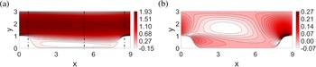
 U(x,y)
 V(x,y)
 Re=100
 U(x,y)
 V(x,y)
 Re=190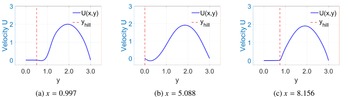
 U(x,y)
 yhill(x)
 Re=100
 x=0.997
 x=5.088
 x=8.156
 U(x,y)
 t=800
t=800 yhill(x)
 Re=190
 x=0.914
 x=4.664
 x=8.414
 f^x(x,y)
 f^y(x,y)
 f^z(x,y)
 kz=0.55
 Re=100
 u^(x,y)
 v^(x,y)
 w^(x,y)
 kz=0.55
 Re=100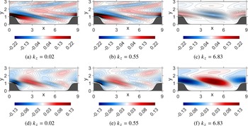
 f^x(x,y)
 f^y(x,y)
 Re=100
 ω=1
ω=1
 u^(x,y)
 v^(x,y)
 Re=100
 ω=1
ω=1
 u^(x,y)
 v^(x,y)
 Re=100
 ω=0.45
 u^(x,y)
 v^(x,y)
 Re=100
 ω=−0.09
 f^x(x,y)
 Re=190
 Re=300
 ω=1
ω=1 f^x(x,y)
 Re=190
 f^x(x,y)
 Re=300
 kz=0.55
 u^(x,y)
 Re=190
 Re=300
 ω=1, 0.45
 0.09
0.09 u^(x,y)
 Re=190
 u^(x,y)
 Re=300
 kz=0.55
 f^x(x,y)
 Re=190
 Re=300
 kz=0
kz=0 f^x(x,y)
 Re=190
 f^x(x,y)
 Re=300
 ω=1
ω=1
 u^(x,y)
 Re=190
 Re=300
 kz=0
kz=0 u^(x,y)
 Re=190
 u^(x,y)
 Re=300
 ω=1
ω=1
 σ
σ H
H Re=50
Re=50 Re=100
 Re=190
 kz=[0.02,0.07,0.55,2.94,6.83]
 Re=100
 Re=190
 u^
u^ (Nx,Ny)
 (48×60)
 (60×72)
 (80×96)
 (96×120)
 (108×132)
 Re=100
 kz=0.023
 ω=0.09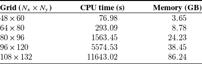
 ω=1.0
ω=1.0 kz=0.55
 Re=100
 Open access

