

1. Introduction
In recent years, China’s declining fertility rate has garnered widespread attention. Since 2016, both fertility and the number of births have declined year by year. The total fertility rate (TFR) fell from 1.7 births per woman in 2016 to 1.07 in 2022, placing China among the lowest-fertility major economies. In 2022, China recorded 9.56 million births and 10.41 million deaths, implying a net population decline of 0.85 million and marking the first episode of negative population growth in nearly six decades. Negative population growth poses significant challenges to socioeconomic development. Therefore, mitigating the decline in fertility and improving population structure are essential for sustaining long-term economic growth and promoting high-quality development.
Fertility inequality is a critical factor contributing to persistently low fertility rates. It refers to the significant divergence in fertility behavior across groups with different economic circumstances (Wietzke, Reference Wietzke2020). In China, a salient manifestation of fertility inequality is the U-shaped relationship between income and fertility (Wu & Zhao, Reference Wu and Zhao2024; Zhu & Hong, Reference Zhu, Hong, Hong, Jiang, Luo and Li2023), where the number of children per family initially declines and then rises as income levels increase. Moreover, applying the middle-income measurement approach proposed by Sicular et al. (Reference Sicular, Yang and Gustafsson2022),Footnote 1 an analysis of the China Family Panel Studies (CFPS) data estimates that approximately 58% of China’s employed population falls within the middle-income bracket. The combination of a large middle-income population and comparatively low fertility among this group constitutes an important contributor to China’s low fertility.
Accordingly, flattening the U-shaped income-fertility pattern and raising fertility intentions among middle-income households are critical to stabilizing the decline in the TFR. Since household human capital is a key determinant of income, this paper focuses on the fertility-inequality phenomenon whereby household human capital and fertility exhibit a U-shaped relationship. From the perspective of complementarity among the inputs required for child educational investment, we illustrate the mechanism through which household human capital generates a U-shaped fertility pattern, and further discuss how weakening this U-shaped structure may help increase fertility and improve long-run demographic balance.
First, drawing on Attanasio et al. (Reference Attanasio, Meghir and Nix2020) and Dzhumashev and Tursunalieva (Reference Dzhumashev and Tursunalieva2023), we develop a theoretical framework in which children’s human capital is produced using multiple inputs – parental time investment, monetary investment, parental human capital, and average human capital in society – and use this framework to analyze how complementarity among educational inputs shapes fertility choices across households with different levels of human capital. The model delivers a clear prediction: when educational inputs are complements, the relationship between household human capital and fertility is U-shaped, with middle-human-capital households exhibiting the lowest fertility; by contrast, when inputs are substitutes, the relationship becomes inverted U-shaped. We then test these implications using the CFPS database. The empirical results indicate that: (i) fertility behavior in China exhibits pronounced heterogeneity in fertility outcomes and household human capital is robustly related to the number of children in a U-shaped manner; (ii) educational inputs are significantly complementary overall, implying that improvements in children’s human capital rely on the joint contribution of multiple inputs; and (iii) both the U-shaped fertility pattern and input complementarity are prevalent across China’s eastern, central, and western regions. Taken together, the theoretical and empirical evidence suggests that under strong complementarity constraints, households must increase both educational time and monetary investment to effectively enhance children’s human capital. This requirement implies that low-human-capital households are more inclined to allocate resources toward childbearing rather than child investment; middle-human-capital households face the strongest pressure from the quantity–quality trade-off and thus exhibit the lowest fertility; and high-human-capital households, being better able to produce higher-quality children, tend to have more children – thereby generating a U-shaped fertility structure. Policies that enhance substitutability among educational inputs may help relieve households’ childrearing cost pressures, mitigate fertility inequality, and ultimately contribute to higher aggregate fertility.
Building on the above analysis, this paper makes two main contributions. First, we study persistently low fertility from the perspective of the societal fertility structure. Unlike much of the existing literature, which explains fertility decline primarily through exogenous determinants of fertility intentions (e.g., housing prices, income, or educational attainment), we use an overlapping-generations (OLG) framework to highlight an internal mechanism through which fertility structure contributes to both low fertility and fertility inequality. Second, focusing on the process of human capital formation, we elucidate how the composition of educational investments affects fertility decisions. Prior studies often attribute the U-shaped relationship between household human capital (or income) and fertility to channels such as women’s occupational choices, fertility timing, or the marketization of childcare and childrearing services (Abad et al., Reference Abad, Etner, Raffin and Seegmuller2025; Hazan & Zoabi, Reference Hazan and Zoabi2015; Yakita, Reference Yakita2018). In contrast, we conceptualize child investment as a production process jointly determined by educational time inputs, monetary inputs, and parental human capital, and emphasize that complementarity among these inputs leads households with different human-capital endowments to face systematically different trade-offs when choosing fertility and child investment. This mechanism endogenously generates U-shaped differences in fertility across human-capital groups and provides a new explanation for fertility inequality at the household level.
The remainder of the paper is organized as follows. Section 2 reviews the related literature. Section 3 presents the fertility-decision model within an OLG framework, derives the relationship between household human capital and fertility, and develops testable hypotheses. Section 4 describes the data, variable construction, and econometric specifications. Section 5 reports and discusses the empirical results. Section 6 concludes and offers policy implications.
2. Literature review
As economic development advances, a sustained decline in the TFR has become a common challenge faced by many countries. Against this backdrop, a growing body of research has examined systematic differences in fertility behavior across households with different socioeconomic status. Using survey data from the United States over 1826–1960, Jones and Tertilt (Reference Jones, Tertilt and Rupert2008) finds a consistently negative association between socioeconomic status and fertility: households with higher socioeconomic status tend to have fewer children. Examining fertility around the Industrial Revolution in the United Kingdom, Clark and Cummins (Reference Clark and Cummins2009) shows that as aggregate fertility declined in the post-Industrial Revolution period, the fertility decline was particularly pronounced among wealthy households. Using Swedish population data spanning 1880–1970, Dribe and Scalone (Reference Dribe and Scalone2014) documents that prior to the fertility transition, fertility was lower among high-status groups than among low-status groups; after the transition began, fertility among the middle-status group fell to the lowest level, well below that of agricultural workers and the elite.
In the Chinese context, as fertility has continued to fall, many studies have documented a distinct U-shaped fertility pattern across socioeconomic groups. Combining theoretical modeling with empirical analysis, Liu and Liu (Reference Liu and Liu2020) finds a significant U-shaped relationship between women’s income and the decision to have a second child following the introduction of China’s universal two-child policy. Zhu and Hong (Reference Zhu, Hong, Hong, Jiang, Luo and Li2023) likewise shows that household income exhibits a U-shaped relationship with second-birth intentions: high-income households exhibit stronger second-birth intentions than low-income households, while middle-income households report the lowest intentions. Using data from the Chinese General Social Survey (CGSS), Wu and Zhao (Reference Wu and Zhao2024) examine how income inequality affects individual fertility intentions. They find that income inequality significantly depresses fertility intentions among middle-income groups but has a positive effect among high-income groups, further corroborating a U-shaped relationship between fertility intentions and income.
To investigate the mechanisms underlying the fertility structure described above, scholars have examined the sources of cross-household differences in fertility decisions from multiple perspectives. The quantity–quality trade-off framework proposed by Becker (Reference Becker1960) has become a standard framework for analyzing household fertility and child-investment choices. In this framework, households make a rational trade-off between the number of children and child “quality”: as income rises, households tend to invest more in child quality, which raises the marginal cost of childbearing and reduces fertility. Building on this insight, Galor and Weil (Reference Galor and Weil2000) uses an OLG framework to argue that economic development increases the returns to educating children, thereby strengthening households’ incentives to invest in child quality and contributing to a long-run decline in fertility. De La Croix and Doepke (Reference Croix and Doepke2003) further develop an OLG model grounded in the quantity–quality trade-off to systematically analyze fertility differences across income groups, showing that high-income households are more inclined to invest in children’s education; because educational investments entail high opportunity costs, fertility among high-income households is relatively lower.
While the quantity–quality trade-off framework helps explain the negative relationship between fertility and household human capital, it has difficulty accounting for the fertility rebound among high-income and high-human-capital households – that is, the observed U-shaped fertility pattern. To address this puzzle, a strand of the literature extends the quantity-quality framework by incorporating mechanisms such as women’s career choices, fertility timing, and the availability provision of childcare and childrearing services. Hazan and Zoabi (Reference Hazan and Zoabi2015) introduce a channel through which households can substitute market-based services (e.g., nannies and domestic help) for parental childcare time and shows that fertility begins to recover once household human capital exceeds a threshold, generating a U-shaped relationship between household human capital and the number of children. Yakita (Reference Yakita2018) embeds women’s occupational choice into a fertility-decision model, arguing that when women’s wages are low, women are more likely to exit the labor force to provide childcare, leading to higher fertility; as women’s market participation and earnings increase, the opportunity cost of childbearing rises sharply and fertility declines; when women’s income reaches a sufficiently high level, households can purchase market childcare services to substitute for parental time, and fertility rebounds. Abad et al. (Reference Abad, Etner, Raffin and Seegmuller2025), focusing on fertility timing, propose that households increasingly postpone childbearing as income rises in order to accumulate human capital; once income becomes sufficiently high, delayed childbearing offsets the earlier decline in early fertility, thereby producing an overall U-shaped fertility pattern.
Although existing studies have documented the nonlinear features of household fertility behavior from multiple perspectives, two issues remain to be further explored. First, much of the literature explains the formation of the U-shaped fertility pattern by introducing exogenous factors that affect fertility – such as the market provision of childcare services, women’s occupational choices, and delayed childbearing – while paying relatively little attention to why, under a given educational environment, households may endogenously develop stable and systematic differences in fertility outcomes. Second, although the quantity–quality trade-off is widely used to analyze fertility decisions, most studies do not explicitly examine the interactions among multiple educational inputs. In particular, they tend to overlook that when these inputs are strongly complementary, households with different levels of human capital face systematically different pressures in balancing quantity and quality, which can endogenously generate a U-shaped fertility structure. Motivated by these gaps, this paper studies fertility inequality through the lens of children’s human capital formation. Following Attanasio et al. (Reference Attanasio, Meghir and Nix2020) and Dzhumashev and Tursunalieva (Reference Dzhumashev and Tursunalieva2023), we model child education as a production process jointly determined by educational time investment, monetary investment, parental human capital, and the social (economy-wide) stock of human capital. We focus on how complementarity among educational inputs amplifies the quantity–quality trade-off and endogenously produces persistent fertility-structure differences across households with different levels of human capital, thereby offering a new mechanism for understanding fertility inequality in the context of persistently low fertility.
3. Theoretical model
This paper develops an OLG model to study fertility and child-investment decisions among households with different levels of human capital. Following Attanasio et al. (Reference Attanasio, Meghir and Nix2020) and Dzhumashev and Tursunalieva (Reference Dzhumashev and Tursunalieva2023), we treat households’ monetary investment in children’s education, time investment, parental human capital, and the economy-wide average level of human capital as key inputs into children’s human capital formation. We specify a CES technology for child human capital production and use the model to examine how complementarity among these inputs affects fertility choices across human-capital groups.
3.1. Model setup
We assume that an individual household’s life consists of two periods: a working period and a retirement period. During the working period, households make both time-allocation and income-allocation decisions. Each household is endowed with one unit of time, which is allocated between labor supply and childcare. Through labor, households with different levels of human capital earn different labor incomes, which are then allocated to consumption, savings, and education expenditures. During the retirement period, households finance consumption using savings accumulated in the working period.
Households derive utility from consumption in the working period, consumption in the retirement period, and the total human capital of all children. Preferences take a log-utility form, so the household’s lifetime utility can be written as: $U{\rm{\;\;}} = {\rm{\;\;ln}}{C_t} + \beta \,{\rm{ln}}{C_{t + 1}} + \rho \,{\rm{ln}}\left( {{N_t}{H_{t + 1}}} \right)$
Here, ${C_t}$
denotes household consumption in the working period;
${C_t}$
denotes household consumption in the working period; ${C_{t + 1}}$
denotes consumption in retirement. Let
${C_{t + 1}}$
denotes consumption in retirement. Let ${N_t}$
be the number of children, and
${N_t}$
be the number of children, and ${H_{t + 1}}$
the human capital of each child. Then
${H_{t + 1}}$
the human capital of each child. Then ${N_t}{H_{t + 1}}$
represents the total human capital of all children. The parameter
${N_t}{H_{t + 1}}$
represents the total human capital of all children. The parameter $\beta $
is the discount factor, and
$\beta $
is the discount factor, and $\rho $
is the altruism parameter capturing the household’s preference for investing in children’s education.
$\rho $
is the altruism parameter capturing the household’s preference for investing in children’s education.
Households invest both time and monetary resources in children in order to raise children’s human capital. Childrearing requires a fixed childcare time cost ( $v$
) and a variable education time input (
$v$
) and a variable education time input ( ${e_t}$
), as well as a monetary input (
${e_t}$
), as well as a monetary input ( ${Q_t}$
).The educational time input (
${Q_t}$
).The educational time input ( ${e_t}$
) and the monetary input (
${e_t}$
) and the monetary input ( ${Q_t}$
) directly affect children’s human capital formation. In addition, parental human capital and the economy-wide average level of human capital also shape children’s human capital (Dzhumashev & Tursunalieva, Reference Dzhumashev and Tursunalieva2023). Accordingly, the child human capital production function is specified as:
${Q_t}$
) directly affect children’s human capital formation. In addition, parental human capital and the economy-wide average level of human capital also shape children’s human capital (Dzhumashev & Tursunalieva, Reference Dzhumashev and Tursunalieva2023). Accordingly, the child human capital production function is specified as: ${H_{t + 1}}\;\; = \;\;{\left( {{\alpha _1}Q_t^\varepsilon + {\alpha _2}e_t^\varepsilon + {\alpha _3}H_t^\varepsilon + {\alpha _4}\bar H_t^\varepsilon } \right)^{{1 \over \varepsilon }}},\;\;\;\;\varepsilon \le 1$
The parameter $\varepsilon $
governs the degree of complementarity among inputs
$\varepsilon $
governs the degree of complementarity among inputs ${Q_t}$
,
${Q_t}$
, ${e_t}$
,
${e_t}$
, ${H_t}$
, and
${H_t}$
, and ${\bar H_t}$
.Footnote
2
${\bar H_t}$
.Footnote
2
We assume that each household is endowed with one unit of time in the working period. Raising children requires a fixed childcare time input of $v{N_t}$
and an education time input of
$v{N_t}$
and an education time input of ${e_t}{N_t}$
. Hence, labor supply in the working period,
${e_t}{N_t}$
. Hence, labor supply in the working period, ${l_t}$
, satisfies:
${l_t}$
, satisfies: ${l_t}{\rm{\;\;}} = {\rm{\;\;}}1 - v{N_t} - {e_t}{N_t}.$
Household consumption in the working period is determined by allocating labor income among current consumption, savings, and monetary expenditures on children’s education. The working-period budget constraint is given by: ${W_t}{H_t}{l_t}{\rm{\;\;}} = {\rm{\;\;}}{C_t} + {S_t} + {N_t}{Q_t}.$
Here, ${W_t}$
denotes the average social wage rate,
${W_t}$
denotes the average social wage rate, ${S_t}$
denotes savings in the working period, and
${S_t}$
denotes savings in the working period, and ${N_t}{Q_t}$
represents the household’s monetary educational spending on
${N_t}{Q_t}$
represents the household’s monetary educational spending on ${N_t}$
children – i.e., market expenditures on education-related goods and services. Greater spending on children’s education crowds out savings and, through the retirement-period budget constraint, affects future consumption.
${N_t}$
children – i.e., market expenditures on education-related goods and services. Greater spending on children’s education crowds out savings and, through the retirement-period budget constraint, affects future consumption.
In the retirement period, households no longer work and finance consumption using savings accumulated in the working period: ${C_{t + 1}}{\rm{\;\;}} = {\rm{\;\;}}{S_t}\left( {1 + {r_{t + 1}}} \right),$
where ${r_{t + 1}}$
is the rate of return on savings.
${r_{t + 1}}$
is the rate of return on savings.
We assume perfectly competitive capital and labor markets. Accordingly, the wage rate ${W_t}$
and the rate of return
${W_t}$
and the rate of return ${r_{t + 1}}$
are taken as exogenous constants. Under this assumption, we analyze fertility and child-investment decisions across households with different levels of human capital. The household utility maximization model is formulated as follows:
${r_{t + 1}}$
are taken as exogenous constants. Under this assumption, we analyze fertility and child-investment decisions across households with different levels of human capital. The household utility maximization model is formulated as follows: $\mathop {{\rm{max}}}\limits_{{N_t},{e_t},{S_t},{Q_t}} {\rm{ln}}{C_t} + \beta \,{\rm{ln}}{C_{t + 1}} + \rho \,{\rm{ln}}\left( {{N_t}{H_{t + 1}}} \right)$
By substituting the budget constraints from Equations (2) to (5) into the utility function and taking partial derivatives with respect to ${S_t}$
,
${S_t}$
, ${N_t}$
,
${N_t}$
, ${e_t}$
, and
${e_t}$
, and ${Q_t}$
, the household’s optimal decision can be derived as follows:
${Q_t}$
, the household’s optimal decision can be derived as follows: ${S_t}\;\; = \;\;{{\beta {W_t}{H_t}} \over {1 + \beta + \rho }}$ ${({Q_t})^{\varepsilon - 1}}\;\; = \;\;{{{\alpha _3}H_t^\varepsilon + {\alpha _4}\bar H_t^\varepsilon } \over {{\alpha _1}v{W_t}{H_t}}}$ ${({e_t})^{\varepsilon - 1}}\;\; = \;\;{{{\alpha _3}H_t^\varepsilon + {\alpha _4}\bar H_t^\varepsilon } \over {{\alpha _2}v}}.$ ${N_t}\;\; = \;\;{\rho \over {v\left( {1 + \rho + \beta } \right)}} \cdot {{{\alpha _3}H_t^\varepsilon + {\alpha _4}\bar H_t^\varepsilon } \over {{\alpha _1}Q_t^\varepsilon + {\alpha _2}e_t^\varepsilon + {\alpha _3}H_t^\varepsilon + {\alpha _4}\bar H_t^\varepsilon }}$
3.2. Analysis of household child-rearing decisions
3.2.1. The impact of household human capital levels on monetary investment in children
Proposition 1 As household human capital increases, the monetary investment in children’s education also rises.
Proof. Taking the partial derivative of Equation (8) with respect to parental human capital levels, we have ${{\partial {Q_t}} \over {\partial {H_t}}}\;\; = \;\;Q_t^{2 - \varepsilon }{{{\alpha _1}{W_t}v\left[ {\left( {1 - \varepsilon } \right){\alpha _3}H_t^\varepsilon + {\alpha _4}\bar H_t^\varepsilon } \right]} \over {\left( {1 - \varepsilon } \right){{({\alpha _1}{W_t}{H_t}v)}^2}}} \gt 0$
That is, for all households, a higher level of household human capital is associated with greater monetary investment in children’s education. The intuition is that high–human-capital households can provide better living conditions for their children and typically choose higher-quality educational arrangements, which raises the associated costs of child investment.
3.2.2. The impact of household human capital levels on time investment
Proposition 2 When the inputs into child education are complements, households increase their time investment in children as household human capital rises. By contrast, when these inputs are substitutes, higher household human capital is associated with lower time investment in children’s education.
Proof. Taking the partial derivative of Equation (9) with respect to parental human capital levels, we have ${{\partial {e_t}} \over {\partial {H_t}}} = e_t^{2 - \varepsilon }{{{\alpha _3}\varepsilon } \over {\left( {\varepsilon - 1} \right){\alpha _2}v}}H_t^{\varepsilon - 1}$
-
If $\varepsilon \lt 0$
,
${{\partial {e_t}} \over {\partial {H_t}}} \gt 0$
, indicating that as household human capital increases, time investment in children’s education also rises.
$\varepsilon \lt 0$
,
${{\partial {e_t}} \over {\partial {H_t}}} \gt 0$
, indicating that as household human capital increases, time investment in children’s education also rises. -
If
$0 \lt \varepsilon \le 1$
,
${{\partial {e_t}} \over {\partial {H_t}}} \le 0$
, implying that as household human capital increases, time investment in children’s education declines.


The underlying mechanism is as follows: when $\varepsilon \lt 0$
, the elasticity of substitution among input factors satisfies
$\varepsilon \lt 0$
, the elasticity of substitution among input factors satisfies $0 \lt {\tilde E_s} \lt 1$
, indicating a complementary relationship between educational input factors. In this case, the accumulation of children’s human capital requires both parental human capital and time investment, making them jointly necessary inputs. In contrast, when
$0 \lt {\tilde E_s} \lt 1$
, indicating a complementary relationship between educational input factors. In this case, the accumulation of children’s human capital requires both parental human capital and time investment, making them jointly necessary inputs. In contrast, when $0 \lt \varepsilon \le 1$
, the elasticity of substitution satisfies
$0 \lt \varepsilon \le 1$
, the elasticity of substitution satisfies ${\tilde E_s} \ge1$
, indicating a substitutive relationship. Under this condition, parental human capital and monetary investment can serve as a substitute for direct time investment in children’s education.
${\tilde E_s} \ge1$
, indicating a substitutive relationship. Under this condition, parental human capital and monetary investment can serve as a substitute for direct time investment in children’s education.
3.2.3. The impact of household human capital levels on the number of children
Proposition 3 When the input factors contributing to children’s human capital formation are complementary, the relationship between household human capital and the number of children follows a U-shaped pattern. Conversely, when these input factors are substitutable, the relationship exhibits an inverted U-shaped pattern.
Proof. Taking the partial derivative of Equation (10) with respect to parental human capital levels, we have: ${{\partial {N_t}} \over {\partial {H_t}}} = {\rho \over {v\left( {1 + \rho + \beta } \right)}}{{\varepsilon \left( {{\alpha _3}H_t^\varepsilon + {\alpha _4}\bar {H}_t^\varepsilon } \right)} \over {\left( {\varepsilon - 1} \right){{\left( {{\alpha _1}Q_t^\varepsilon + {\alpha _2}e_t^\varepsilon + {\alpha _3}H_t^\varepsilon + {\alpha _4}\bar H_t^\varepsilon } \right)}^2}}}A$
where
 $$A = {{{\alpha _4}{\mkern 1mu} {{{\bar{\,H_t}} }^{{\kern 1pt} \varepsilon }}} \over {{W_t}{\mkern 1mu} v{\mkern 1mu} H_t^2}}{\mkern 1mu} \,{Q_t} - {{{\alpha _3}H_t^{\varepsilon - 1}} \over v}{\mkern 1mu} {e_t}$$
. Furthermore, when
$$A = {{{\alpha _4}{\mkern 1mu} {{{\bar{\,H_t}} }^{{\kern 1pt} \varepsilon }}} \over {{W_t}{\mkern 1mu} v{\mkern 1mu} H_t^2}}{\mkern 1mu} \,{Q_t} - {{{\alpha _3}H_t^{\varepsilon - 1}} \over v}{\mkern 1mu} {e_t}$$
. Furthermore, when $A = 0$
,
$A = 0$
,
 $${H_t} ={\hat H_t}$$
 $$ = {\left( {{{\left( {{{{\alpha _1}} \over {{\alpha _2}}}} \right)}^{{1 \over {\varepsilon - 1}}}}{{{\alpha _3}} \over {{\alpha _4}}}W_t^{{\varepsilon \over {\varepsilon - 1}}}{{\bar H}_t}^{ - \varepsilon }} \right)^{{{1 - \varepsilon } \over {{\varepsilon ^2}}}}}$$
.
$$ = {\left( {{{\left( {{{{\alpha _1}} \over {{\alpha _2}}}} \right)}^{{1 \over {\varepsilon - 1}}}}{{{\alpha _3}} \over {{\alpha _4}}}W_t^{{\varepsilon \over {\varepsilon - 1}}}{{\bar H}_t}^{ - \varepsilon }} \right)^{{{1 - \varepsilon } \over {{\varepsilon ^2}}}}}$$
.
-
If
$\varepsilon \lt 0$
, then:-
– When
${H_t} \lt {\widehat H_t}$
,
$A \lt 0,$
and
${{\partial {N_t}} \over {\partial {H_t}}} \lt 0$
, indicating that an increase in household human capital reduces the number of children. -
– When
${H_t} \gt {\widehat H_t}$
,
$A \gt 0,$
and
${{\partial {N_t}} \over {\partial {H_t}}} \gt 0$
, indicating that an increase in household human capital raises the number of children. -
– This implies a U-shaped relationship between household human capital and the number of children.
-
-
If
$0 \le \varepsilon \le 1$
, then:-
– When
${H_t} \lt {\widehat H_t}$
,
$A \lt 0,$
and
${{\partial {N_t}} \over {\partial {H_t}}} \gt 0$
, implying that an increase in household human capital raises the number of children. -
– When
${H_t} \gt {\widehat H_t}$
,
$A \gt 0,$
and
${{\partial {N_t}} \over {\partial {H_t}}} \lt 0$
, implying that an increase in household human capital reduces the number of children. -
– This results in an inverted U-shaped relationship between household human capital and the number of children.
-


To understand the mechanism behind the above findings, we further analyze the problem through the lens of the quantity–quality trade-off. Differentiating fertility with respect to children’s human capital yields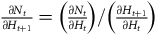 ${{\partial {N_t}} \over {\partial {H_{t + 1}}}} = \left( {{{\partial {N_t}} \over {\partial {H_t}}}} \right)/\left( {{{\partial {H_{t + 1}}} \over {\partial {H_t}}}} \right)$
. Since
${{\partial {N_t}} \over {\partial {H_{t + 1}}}} = \left( {{{\partial {N_t}} \over {\partial {H_t}}}} \right)/\left( {{{\partial {H_{t + 1}}} \over {\partial {H_t}}}} \right)$
. Since ${{\partial {H_{t + 1}}} \over {\partial {H_t}}} \gt 0$
, the sign of
${{\partial {H_{t + 1}}} \over {\partial {H_t}}} \gt 0$
, the sign of ${{\partial {N_t}} \over {\partial {H_{t + 1}}}}$
is the same as that of
${{\partial {N_t}} \over {\partial {H_{t + 1}}}}$
is the same as that of ${{\partial {N_t}} \over {\partial {H_t}}}$
.
${{\partial {N_t}} \over {\partial {H_t}}}$
.
When $\varepsilon \lt 0$
, the inputs required to raise children’s human capital are complements. If
$\varepsilon \lt 0$
, the inputs required to raise children’s human capital are complements. If ${H_t} \lt {\widehat H_t}$
, then
${H_t} \lt {\widehat H_t}$
, then ${{\partial {N_t}} \over {\partial {H_{t + 1}}}} \lt 0$
. A complementary educational technology requires multiple inputs to be scaled up jointly. As a result, low–human-capital households tend to choose childbearing rather than intensive child investment, whereas middle–human-capital households reduce fertility in order to invest more in children. If
${{\partial {N_t}} \over {\partial {H_{t + 1}}}} \lt 0$
. A complementary educational technology requires multiple inputs to be scaled up jointly. As a result, low–human-capital households tend to choose childbearing rather than intensive child investment, whereas middle–human-capital households reduce fertility in order to invest more in children. If ${H_t} \gt {\widehat H_t}$
, then
${H_t} \gt {\widehat H_t}$
, then ${{\partial {N_t}} \over {\partial {H_{t + 1}}}} \gt 0$
. In this region, complementarity enables high–human-capital households to produce higher-quality children, which in turn encourages them to have more children.
${{\partial {N_t}} \over {\partial {H_{t + 1}}}} \gt 0$
. In this region, complementarity enables high–human-capital households to produce higher-quality children, which in turn encourages them to have more children.
When $0 \le \varepsilon \le 1$
, the inputs required to raise children’s human capital are substitutes. If
$0 \le \varepsilon \le 1$
, the inputs required to raise children’s human capital are substitutes. If ${H_t} \lt {\widehat H_t}$
, then
${H_t} \lt {\widehat H_t}$
, then ${{\partial {N_t}} \over {\partial {H_{t + 1}}}} \gt 0$
. Under a substitutable technology, households can increase their human capital and monetary inputs to substitute for parental time devoted to educating children; consequently, fertility increases as household human capital rises. If
${{\partial {N_t}} \over {\partial {H_{t + 1}}}} \gt 0$
. Under a substitutable technology, households can increase their human capital and monetary inputs to substitute for parental time devoted to educating children; consequently, fertility increases as household human capital rises. If ${H_t} \gt {\widehat H_t}$
, then
${H_t} \gt {\widehat H_t}$
, then ${{\partial {N_t}} \over {\partial {H_{t + 1}}}} \lt 0$
. In this region, substitutability allows higher–human-capital households to rely heavily on monetary inputs to substitute for time inputs; the resulting high cost of child investment leads fertility to decline as household human capital rises.
${{\partial {N_t}} \over {\partial {H_{t + 1}}}} \lt 0$
. In this region, substitutability allows higher–human-capital households to rely heavily on monetary inputs to substitute for time inputs; the resulting high cost of child investment leads fertility to decline as household human capital rises.
3.3. Research hypotheses
Based on the theoretical analysis above, we propose the following hypotheses and conduct empirical tests:
Hypothesis 1: Household human capital is positively associated with monetary investment in children’s education: households with higher human capital spend more on children’s education.
Hypothesis 2a: When educational inputs are complementary, household human capital is positively associated with time investment in children’s education: households with higher human capital devote more time to educating children.
Hypothesis 2b: When educational inputs are substitutable, household human capital is negatively associated with time investment in children’s education: households with higher human capital devote less time to educating children.
Hypothesis 3a: When the inputs into children’s human capital formation are complementary, household human capital and fertility exhibit a U-shaped relationship: as household human capital rises, the number of children first decreases and then increases.
Hypothesis 3b: When the inputs into children’s human capital formation are substitutable, household human capital and fertility exhibit an inverted U-shaped relationship: as household human capital rises, the number of children first increases and then decreases.
4. Data and empirical model
4.1. Description of data and variables
The data used in this study are drawn from the CFPS. CFPS is a nationally representative longitudinal survey conducted biennially. The sample covers 25 provinces and represents approximately 95% of China’s population. CFPS adopts a multistage stratified sampling design, with sampled households distributed across 25 provinces, 80 cities/prefectures, 144 counties/districts, and 43,805 villages/urban communities, with a target sample size of about 16,000 households. The CFPS contains five main modules – community, household, household members, adults, and children – providing rich information on the dynamics of Chinese households’ economic conditions, demographic structure, educational attainment, and health status.
4.1.1. Dependent variables
Consistent with the theoretical model and the hypotheses, we focus on fertility and child-education investment decisions across households with different levels of human capital. For household fertility decisions, the dependent variable is the number of children in the household. The CFPS 2020 records a unique identifier for each child in the household; by matching household records with child records, we compute the total number of children for each household.
For household education decisions, the dependent variable is children’s human capital. Following Dai and Li (Reference Dai and Li2022) and Wu and Zhang (Reference Wu and Zhang2024), we use children’s Chinese-language and mathematics performance to proxy comprehension ability and logical reasoning ability, respectively. In the CFPS child module, academic performance is reported on a four-point scale (“poor” = 1, “average” = 2, “good” = 3, and “excellent” = 4). Based on these measures, we construct a composite index of children’s human capital by applying the entropy-weight method to Chinese and mathematics scores.
In addition, to further examine how household human capital affects monetary and time investments in children’s education, we measure educational time investment using the CFPS child-module item on “weekly hours spent helping with homework,” and measure monetary investment using the natural logarithm of “total household educational expenditures over the past 12 months + 1.”
4.1.2. Core explanatory variables
The key explanatory variable in this study is household human capital. Existing research (Epo et al., Reference Epo, Baye, Mwabu, Manda, Ajakaiye and Kipruto2025; Su & Guo, Reference Su and Guo2022) typically measures parental human capital along three dimensions: education, health, and work-related characteristics. Following the approach of Su and Guo (Reference Su and Guo2022), we construct an individual-level human capital index based on education, health, and work experience using the entropy-weight method, and then aggregate to the household level by taking the average of the parents’ human capital indices, yielding our measure of household human capital.
Specifically, for the education dimension, we use the highest completed years of schooling reported in the CFPS 2020 individual module, coded as: illiterate = 0, primary school = 6, junior high school = 9, high school = 12, junior college = 15, bachelor’s degree = 16, master’s degree = 19, and PhD = 21. For the health dimension, we use self-rated health, coded as: very healthy = 1, healthy = 2, relatively healthy = 3, fair = 4, and unhealthy = 5. For the work-experience dimension, following Su and Guo (Reference Su and Guo2022), we proxy actual years of work experience as (age-years of schooling-6).
4.1.3. Control variables
Following Ning et al. (Reference Ning, Tang, Huang, Tan, Lin and Sun2022) and Singletary et al. (Reference Singletary, Justice, Baker, Lin, Purtell and Schmeer2022), we include a set of control variables capturing child characteristics, household characteristics, and regional characteristics to more accurately identify household fertility and education decisions.
For household characteristics, we control for parents’ education, parents’ health, parents’ employment status, and residential location. Parents’ education is measured as the maximum years of schooling between the two parents. Parents’ health is constructed from self-rated health: it equals 1 if at least one parent reports being healthy, and 0 otherwise. Parents’ employment status is based on the CFPS 2020 classification of occupational status; we take the household-level average of parents’ employment indicators to capture overall parental employment. Residential location is controlled for using an urban–rural dummy, equal to 1 for urban households and 0 for rural households.
For child characteristics, in households with multiple children, child age is measured as the average age of all children. For regional characteristics, we include province fixed effects to absorb systematic cross-province differences in economic development, public service provision, and fertility- and education-related policies.
Detailed variable definitions are reported in Table 1.
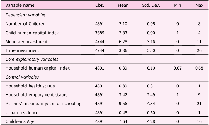
Descriptive statistics of variables

Table 1 Long description
The table presents descriptive statistics of variables related to children and households. It includes three main categories: dependent variables, core explanatory variables, and control variables. The table has 12 rows and 6 columns. Column headers are Variable name, Obs., Mean, Std. Dev., Min, and Max. Row labels are grouped under the three main categories. Row 1: Number of Children, 4891, 2.10, 0.95, 0, 8. Row 2: Child human capital index, 3685, 2.83, 0.90, 1, 4. Row 3: Monetary investment, 4744, 6.28, 3.16, 0, 11. Row 4: Time investment, 4744, 3.86, 5.50, 0, 26. Row 5: Household human capital index, 4891, 0.39, 0.10, 0.07, 0.68. Row 6: Household health status, 4891, 0.89, 0.31, 0, 1. Row 7: Household employment status, 4891, 3.42, 2.49, 1, 9. Row 8: Parents' maximum years of schooling, 4891, 9.56, 4.34, 0, 21. Row 9: Urban residence, 4891, 0.48, 0.50, 0, 1. Row 10: Children's Age, 4891, 7.64, 4.28, 0, 16.
4.2. Empirical model
4.2.1. Regression model for household fertility
To analyze fertility patterns across households with different levels of human capital, we estimate the following baseline model: $n\_chil{d_i} = {\beta _0} + {\beta _1}capita{l_i} + {\beta _2}capital_i^2 + {\beta _3}{X_i} + {\mu _i}$
The dependent variable $n\_chil{d_i}$
denotes the number of children in household
$n\_chil{d_i}$
denotes the number of children in household $i$
. Since the number of children is a nonnegative count outcome, we estimate Equation (14) using a Poisson model. Motivated by the theoretical predictions, household human capital and fertility may exhibit a nonlinear (U-shaped or inverted-U-shaped) relationship; we therefore include both household human capital
$i$
. Since the number of children is a nonnegative count outcome, we estimate Equation (14) using a Poisson model. Motivated by the theoretical predictions, household human capital and fertility may exhibit a nonlinear (U-shaped or inverted-U-shaped) relationship; we therefore include both household human capital $capita{l_i}$
and its squared term
$capita{l_i}$
and its squared term $capital_i^2$
. The vector
$capital_i^2$
. The vector ${X_i}$
includes a set of control variables capturing child characteristics, household characteristics, and the regression also controls for province fixed effects.
${X_i}$
includes a set of control variables capturing child characteristics, household characteristics, and the regression also controls for province fixed effects. ${\mu _i}$
is an error term.
${\mu _i}$
is an error term.
4.2.2. Regression model for household education investment
To further examine how household human capital affects the mode of educational investment, we specify separate regressions for monetary and time investments in children’s education: $mone{y_i} = {\beta _0} + {\beta _1}capita{l_i} + {\beta _2}ag{e_i} + {\beta _3}age_i^2 + {\beta _4}{X_i} + {\mu _i}$ $tim{e_i} = {\beta _0} + {\beta _1}capita{l_i} + {\beta _2}ag{e_i} + {\beta _3}age_i^2 + {\beta _4}{X_i} + {\mu _i}$
The dependent variables $mone{y_i}$
and
$mone{y_i}$
and $tim{e_i}$
denote household
$tim{e_i}$
denote household $i$
’s monetary and time investments in children’s education, respectively. Descriptive statistics show that approximately 16.7% of households report zero monetary educational spending and about 50.39% report zero educational time input. Because educational investment is an active household choice, these zeros are not merely due to censoring or missing values; rather, they carry meaningful economic content. We therefore estimate Equations (15) and (16) using Poisson pseudo-maximum likelihood (PPML), which is well suited to outcomes with a large mass at zero and is robust to heteroskedasticity.
$i$
’s monetary and time investments in children’s education, respectively. Descriptive statistics show that approximately 16.7% of households report zero monetary educational spending and about 50.39% report zero educational time input. Because educational investment is an active household choice, these zeros are not merely due to censoring or missing values; rather, they carry meaningful economic content. We therefore estimate Equations (15) and (16) using Poisson pseudo-maximum likelihood (PPML), which is well suited to outcomes with a large mass at zero and is robust to heteroskedasticity.
Moreover, during primary and lower-secondary schooling, households typically devote substantial time to homework assistance and incur higher educational expenditures. Educational time and monetary inputs may therefore vary with children’s age in an inverted-U-shaped manner. Accordingly, we include children’s age $ag{e_i}$
and its squared term
$ag{e_i}$
and its squared term $age_i^2$
in Equations (15) and (16). The vector
$age_i^2$
in Equations (15) and (16). The vector ${X_i}$
includes additional household- and province-level controls, and
${X_i}$
includes additional household- and province-level controls, and ${\mu _i}$
is an error term.
${\mu _i}$
is an error term.
4.2.3. Regression model for children’s CES human-capital production function
To quantify substitutability versus complementarity among educational inputs, we further specify a CES-type child human-capital production function: ${\rm{ln}}\left( {child\_capita{l_i}} \right) = {1 \over \varepsilon }{\rm{ln}}\left( {{\alpha _1}money_i^\varepsilon + {\alpha _2}time_i^\varepsilon + {\alpha _3}capital_i^\varepsilon + {\alpha _4}avg\_capita{l^\varepsilon }} \right) + {\mu _i}$
The dependent variable ${\rm{ln}}\left( {child\_capita{l_i}} \right)$
is the log human capital level of child
${\rm{ln}}\left( {child\_capita{l_i}} \right)$
is the log human capital level of child $i$
. The variables
$i$
. The variables $mone{y_i}$
and
$mone{y_i}$
and $tim{e_i}$
denote the household’s monetary and time investments in education,
$tim{e_i}$
denote the household’s monetary and time investments in education, $capita{l_i}$
is household human capital, and
$capita{l_i}$
is household human capital, and $avg\_capital$
is the economy-wide average level of human capital capturing the external human-capital environment. The parameter
$avg\_capital$
is the economy-wide average level of human capital capturing the external human-capital environment. The parameter $\varepsilon $
governs the degree of substitutability (or complementarity) among inputs in the CES technology, and
$\varepsilon $
governs the degree of substitutability (or complementarity) among inputs in the CES technology, and ${\mu _i}$
is an error term.
${\mu _i}$
is an error term.
Following the estimation strategies for CES functions in Koesler and Schymura (Reference Koesler and Schymura2015) and Attanasio et al. (Reference Attanasio, Meghir and Nix2020), we estimate Equation (17) using nonlinear least squares (NLS) to identify the substitutability or complementarity among educational inputs.
5. Empirical results
5.1. Baseline regression results
5.1.1. Regression results for the number of children
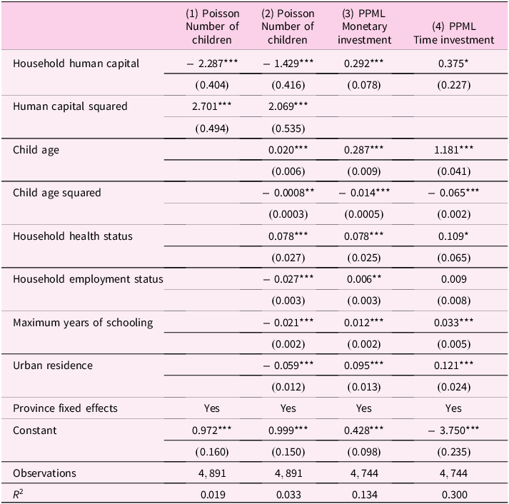
We first examine the effect of household human capital on fertility using the baseline specification in Equation (14). The corresponding estimates are reported in Table 2, columns (1) and (2). Column (1) presents results without any control variables, while column (2) adds a full set of controls, including child characteristics, household characteristics, and province fixed effects.
Estimation results of baseline regression
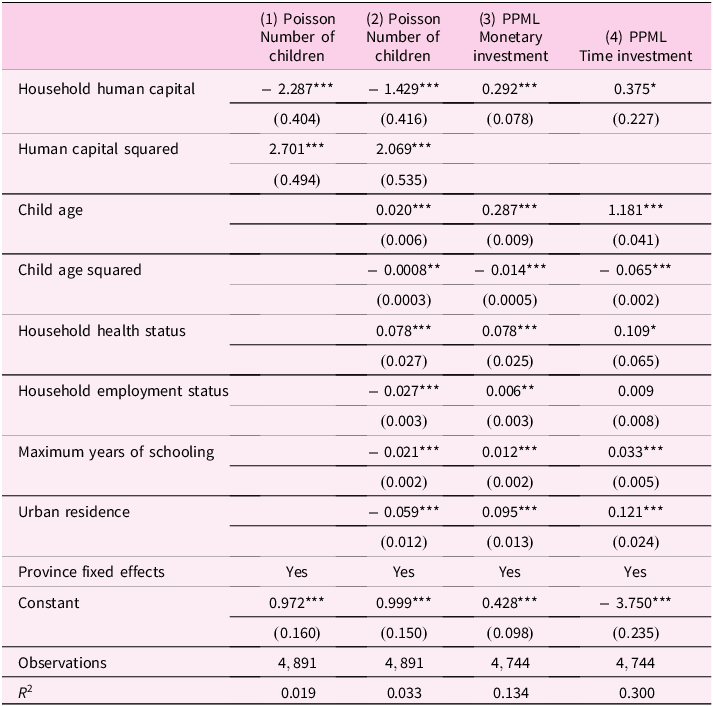
Table 2 Long description
A table with 10 rows and 8 columns showing estimation results of baseline regression. The columns are labeled as (1) Poisson Number of children, (2) Poisson Number of children, (3) PPML Monetary investment, and (4) PPML Time investment. The rows are labeled as Household human capital, Human capital squared, Child age, Child age squared, Household health status, Household employment status, Maximum years of schooling, Urban residence, Province fixed effects, and Constant. Each cell contains numerical values with standard errors in parentheses. Notable trends include significant negative values for Household human capital in columns (1) and (2), and significant positive values for Child age in columns (2), (3), and (4).
Notes: Robust standard errors are reported in parentheses. ***, **, and * denote significance at the 1%, 5%, and 10% levels, respectively.
As shown in Table 2, in column (1), the estimated coefficient on household human capital is -2.287 and the coefficient on its squared term is 2.701; both are statistically significant at the 1% level. After adding the control variables in column (2), the signs and statistical significance of household human capital and its squared term remain stable. These results indicate a significant U-shaped relationship between household human capital and fertility: as household human capital increases, the number of children first decreases and then increases.
Turning to the control variables, the estimates suggest that, holding other factors constant, households with better health status tend to have more children. In contrast, households with better employment status and higher parental education have fewer children. Moreover, rural households have significantly more children than urban households.
5.1.2. Regression results for monetary and time investments in children’s education
Based on the baseline specifications in Equations (15) and (16), we further examine how household human capital affects households’ monetary and time investments in children’s education. The corresponding estimates are reported in Table 2, columns (3) and (4). Column (3) captures the effect of household human capital on monetary educational investment, while column (4) reports the effect on time investment.
As shown in Table 2, column (3), the estimated coefficient on household human capital is 0.292 and is statistically significant at the 1% level, indicating that households with higher human capital spend more on children’s education. This finding supports Hypothesis 1, suggesting a significant positive association between household human capital and monetary educational investment.
In Table 2, column (4), the coefficient on household human capital is 0.375 and is significant at the 10% level, implying that educational time investment also increases with household human capital. However, patterns in input choices alone are not sufficient to determine whether different educational inputs are substitutes or complements. To identify substitutability versus complementarity, we further estimate the child human capital production function.
5.1.3. Estimation results for the child human capital production function
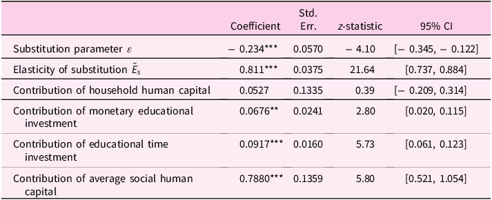
Based on Equation (17), we estimate the CES-type child human capital production function using NLS. The estimation results are reported in Table 3.
Estimation results for the child human capital production function

Table 3 Long description
A table with seven rows and five columns. The columns are labeled Coefficient, Std. Err., z-statistic, and 95% CI. The rows are labeled Substitution parameter epsilon, Elasticity of substitution E sub s, Contribution of household human capital, Contribution of monetary educational investment, Contribution of educational time investment, and Contribution of average social human capital. Each row contains values for Coefficient, Std. Err., z-statistic, and 95% CI. The table presents statistical data related to the estimation results for the child human capital production function.
Notes: *** and ** denote significance at the 1% and 5% levels, respectively.
Table 3 indicates that specifying the CES function as the technology for children’s human capital formation is empirically reasonable. The estimated value of the substitution parameter $\varepsilon $
is −0.234, which is statistically significantly below zero. The implied elasticity of substitution,
$\varepsilon $
is −0.234, which is statistically significantly below zero. The implied elasticity of substitution, $\tilde E$
, is 0.811, significantly less than one, indicating strong complementarity among household human capital, educational time investment, and educational monetary investment. Examining the relative contributions of each input to children’s human capital, educational time investment contributes the most, followed by monetary investment, while the direct contribution of household human capital is comparatively smaller.
$\tilde E$
, is 0.811, significantly less than one, indicating strong complementarity among household human capital, educational time investment, and educational monetary investment. Examining the relative contributions of each input to children’s human capital, educational time investment contributes the most, followed by monetary investment, while the direct contribution of household human capital is comparatively smaller.
Taken together with the earlier regression results for fertility and educational time investment, Table 2 column (4) and Table 3 jointly support Hypothesis 2a: when educational inputs are complementary, households with higher human capital devote more time to children’s education. Moreover, Table 2 column (2) and Table 3 together provide evidence consistent with Hypothesis 3a: under complementarity in the inputs to children’s human capital formation, household human capital and fertility exhibit a U-shaped relationship – fertility first declines and then increases as household human capital rises.
5.2. Robustness test
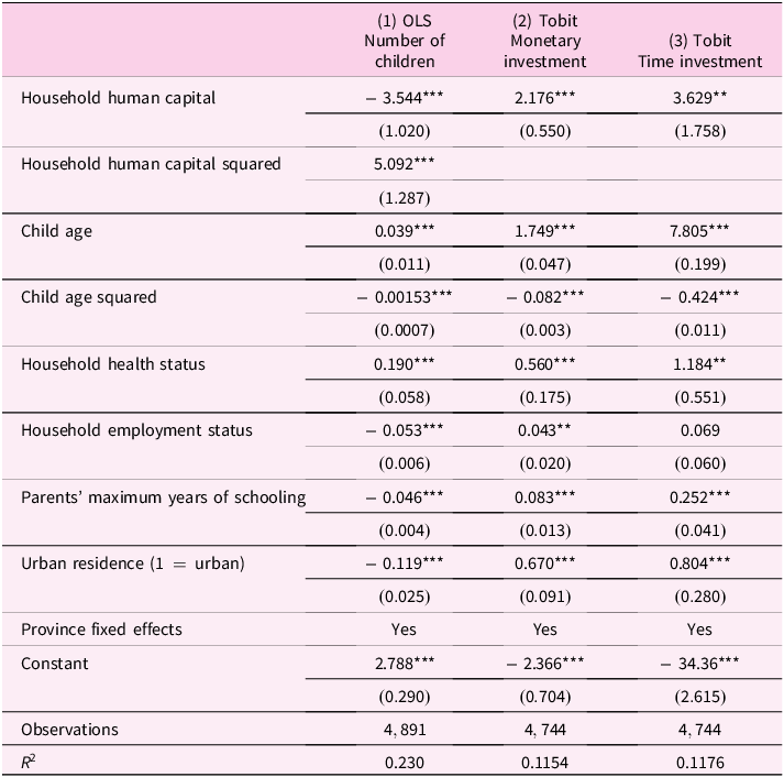
To assess the robustness of the baseline results, we re-estimate the effects of household human capital on fertility and child-investment behavior using alternative econometric specifications. The corresponding results are summarized in Table 4. Column (1) of Table 4 reports an ordinary least squares (OLS) regression of the number of children on household human capital. The OLS estimates show that the coefficient on household human capital remains negative while the coefficient on its squared term remains positive, and both are statistically significant at the 1% level. This implies that the U-shaped relationship between household human capital and fertility persists under OLS, suggesting that the nonlinearity documented in the baseline analysis is highly robust.
Robustness check results

Table 4 Long description
A table with three columns and eleven rows. The columns are labeled as follows: (1) OLS Number of children, (2) Tobit Monetary investment, and (3) Tobit Time investment. The rows are labeled with different variables: Household human capital, Household human capital squared, Child age, Child age squared, Household health status, Household employment status, Parents’ maximum years of schooling, Urban residence (1 = urban), Province fixed effects, Constant, Observations, and R-squared. Each cell contains numerical values representing the coefficients and standard errors for each variable. The table shows the impact of household human capital on the number of children, monetary investment, and time investment, with various statistical significance levels indicated by asterisks.
Notes: Robust standard errors are reported in parentheses. *** and ** denote significance at the 1% and 5% levels, respectively.
Columns (2) and (3) of Table 4 further estimate monetary and time investments in children’s education using Tobit models to examine the robustness of the education-investment results. The estimates indicate that household human capital enters positively in both Tobit specifications, with statistical significance broadly consistent with the baseline PPML results in columns (3) and (4) of Table 2. These findings suggest that households with higher human capital invest more in both the monetary and time dimensions of child education, providing additional support for the robustness of the positive association between household human capital and educational investments.
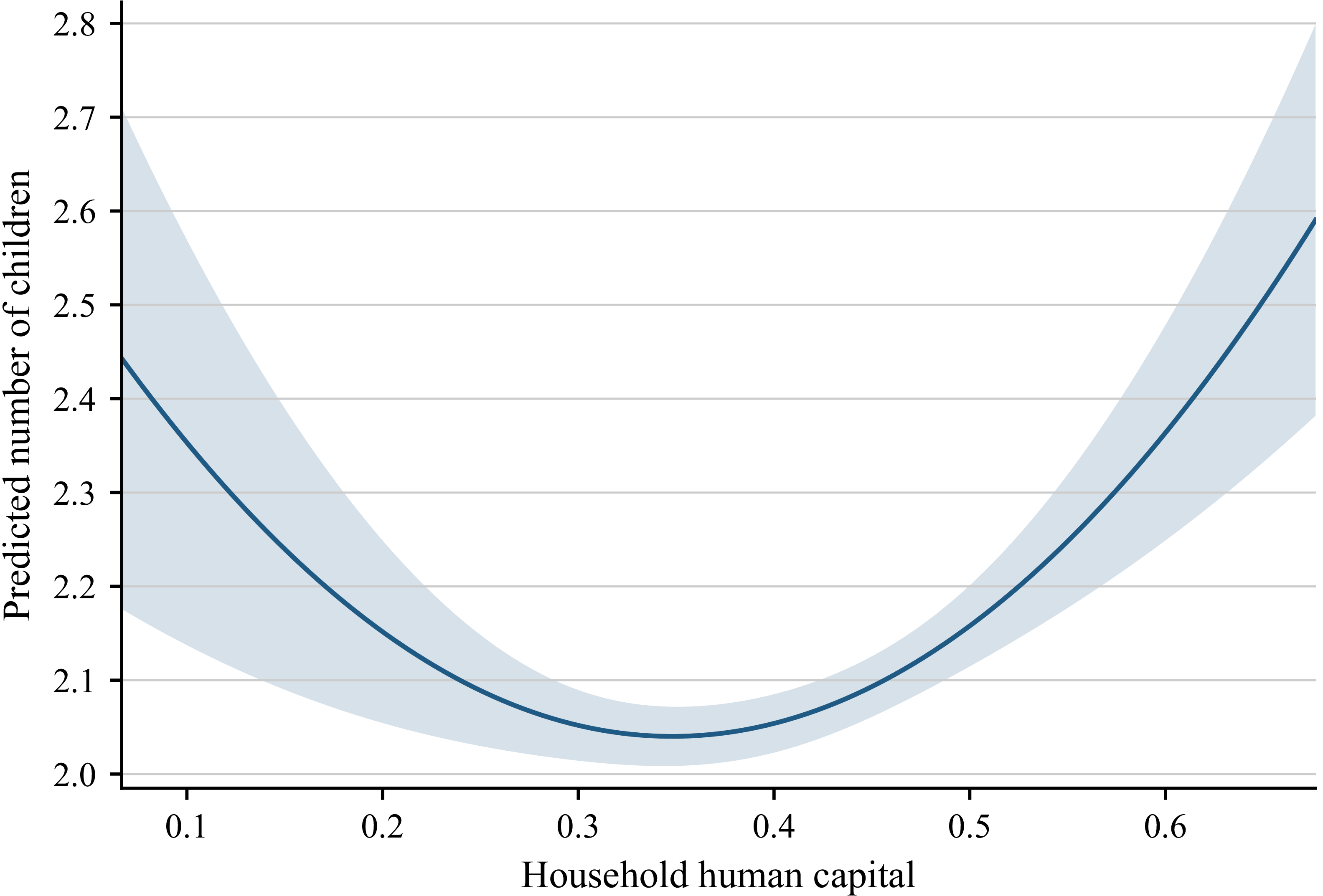
To illustrate more intuitively the robust nonlinear relationship between household human capital and the number of children, Figure 1 plots the predicted relationship between household human capital and fertility based on the OLS estimates reported in Table 4, column (1), together with the corresponding 95% confidence interval. The figure shows that, as household human capital increases, the number of children first declines and then rises, exhibiting a clear U-shaped pattern overall. This graphical evidence is consistent with the baseline and robustness results reported above and further confirms the robustness of the U-shaped relationship between household human capital and fertility.
Predicted number of children by household human capital.

5.3. Heterogeneity analysis
5.3.1. Grouped regressions by household human capital
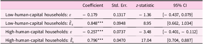
The baseline and robustness results presented above already provide strong evidence of a robust U-shaped relationship between household human capital and the number of children. Accordingly, we further examine whether the complementarity among educational inputs remains consistent across households with different human-capital endowments. Specifically, we use the estimated minimum point of the U-shaped relationship in Table 2, column (2), denoted by $H{C^{\rm{*}}}$
, as the threshold to divide the sample into low and high-human-capital households, and then estimate the CES production function separately for the two subsamples. The corresponding results are reported in Table 5.
$H{C^{\rm{*}}}$
, as the threshold to divide the sample into low and high-human-capital households, and then estimate the CES production function separately for the two subsamples. The corresponding results are reported in Table 5.
Estimated substitution elasticities of educational inputs

Table 5 Long description
A table with four rows and four columns comparing substitution elasticities for low and high-human-capital households. The columns are labeled Coefficient, Std. Err., z-statistic, and 95% CI. The rows are labeled Low-human-capital households: ε, Low-human-capital households: Ês, High-human-capital households: ε, and High-human-capital households: Ês. Row 1: Coefficient, -0.179; Std. Err., 0.1317; z-statistic, -1.36; 95% CI, [-0.437, 0.079]. Row 2: Coefficient, 0.848***; Std. Err., 0.0948; z-statistic, 8.95; 95% CI, [0.662, 1.034]. Row 3: Coefficient, -0.257***; Std. Err., 0.0737; z-statistic, -3.48; 95% CI, [-0.401, -0.112]. Row 4: Coefficient, 0.796***; Std. Err., 0.0470; z-statistic, 17.04; 95% CI, [0.704, 0.887].
Notes: Robust standard errors are reported in parentheses. *** denotes significance at the 1% levels.
Table 5 shows that the estimated elasticities of substitution are below one in both subsamples, indicating that educational time inputs, monetary inputs, and household human capital are complementary across different household human-capital groups. This input structure substantially intensifies the quantity-quality trade-off faced by low-human-capital households, so that within the low-human-capital range, fertility declines as household human capital increases. By contrast, high-human-capital households are better able to produce higher-quality children; therefore, within the high-human-capital range, fertility tends to increase as household human capital rises further.
5.3.2. Grouped regressions by region (Eastern, Central, and Western China)
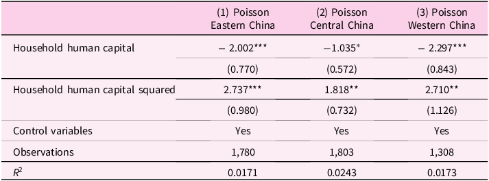
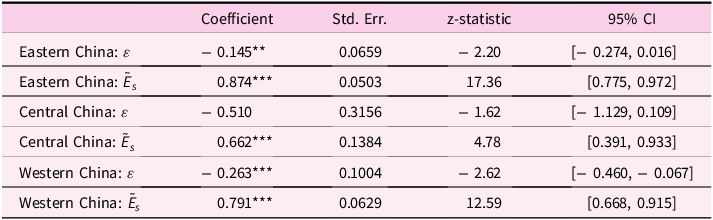
Building on the subgroup analysis above, we further split the sample into China’s eastern, central, and western regions to examine whether (i) the U-shaped relationship between household human capital and the number of children and (ii) complementarity among educational inputs are prevalent across regions. The corresponding results are reported in Tables 6 and 7.
Heterogeneous effects of household human capital on fertility

Table 6 Long description
A table comparing the effects of household human capital on the number of children across different regions in China. The table has three columns and four rows. Column headers are Poisson Eastern China, Poisson Central China, and Poisson Western China. Row labels are Household human capital, Household human capital squared, Control variables, Observations, and R squared. Row 1: Household human capital, -2.002***, -1.035*, -2.297***, (0.770), (0.572), (0.843). Row 2: Household human capital squared, 2.737***, 1.818**, 2.710**, (0.980), (0.732), (1.126). Row 3: Control variables, Yes, Yes, Yes. Row 4: Observations, 1,780, 1,803, 1,308. Row 5: R squared, 0.0171, 0.0243, 0.0173.
Notes: See Table 2.
Estimated substitution elasticities of educational inputs

Table 7 Long description
A table with six rows and four columns comparing estimated substitution elasticities of educational inputs across regions in China. The columns are labeled Coefficient, Std. Err., z-statistic, and 95% CI. The rows are labeled Eastern China: ε, Eastern China: Ẽs, Central China: ε, Central China: Ẽs, Western China: ε, and Western China: Ẽs. Row 1: Coefficient, -0.145; Std. Err., 0.0659; z-statistic, -2.20; 95% CI, [-0.274, 0.016]. Row 2: Coefficient, 0.874; Std. Err., 0.0503; z-statistic, 17.36; 95% CI, [0.775, 0.972]. Row 3: Coefficient, -0.510; Std. Err., 0.3156; z-statistic, -1.62; 95% CI, [-1.129, 0.109]. Row 4: Coefficient, 0.662; Std. Err., 0.1384; z-statistic, 4.78; 95% CI, [0.391, 0.933]. Row 5: Coefficient, -0.263; Std. Err., 0.1004; z-statistic, -2.62; 95% CI, [-0.460, -0.067]. Row 6: Coefficient, 0.791; Std. Err., 0.0629; z-statistic, 12.59; 95% CI, [0.668, 0.915].
Notes: Robust standard errors are reported in parentheses. *** and ** denote significance at the 1% and 5% levels, respectively.
Table 6 shows that, in all three regional subsamples, household human capital exhibits a consistent nonlinear pattern – the linear term is negative and the squared term is positive – and most coefficients are statistically significant at conventional levels. This suggests that the U-shaped relationship between household human capital and fertility is broadly consistent across regions. In terms of magnitude, the coefficient on the squared term is relatively larger in the eastern and western regions, indicating a more pronounced degree of nonlinearity in fertility patterns, whereas the curvature of the U-shape is comparatively flatter in the central region. In addition, Table 7 reports that the estimated elasticities of substitution among educational inputs are all significantly below one in the eastern, central, and western regions, implying that educational inputs are complementary across regions.
Taken together, these findings indicate a high degree of regional consistency in the U-shaped relationship between household human capital and fertility, and that the complementary structure of educational inputs is likewise pervasive at the regional level. Because raising children’s educational “quality” requires households to jointly allocate parental time and monetary expenditures, this investment mode amplifies differences in the quantity–quality trade-off across households with different levels of human capital. As a result, household fertility behavior endogenously gives rise to a robust U-shaped fertility structure at the micro level.
6. Conclusions and policy implications
Persistently low fertility and the onset of negative population growth have become severe challenges facing China today, and these trends conceal a deeper phenomenon of fertility inequality among Chinese households. Building on an OLG framework, this paper studies fertility and child-investment decisions across households with different levels of human capital and tests the theoretical implications using the 2020 CFPS data. The theoretical analysis shows that when educational inputs are complementary, the relationship between household human capital and the number of children is U-shaped, with middle-human-capital households exhibiting lower fertility than other groups; by contrast, when educational inputs are substitutable, the relationship becomes inverted U-shaped. Empirical evidence grounded in this framework further indicates that: (i) fertility inequality is pronounced in China, as reflected in a robust U-shaped relationship between household human capital and fertility, and this pattern holds across subsamples from eastern, central, and western China; and (ii) educational inputs exhibit significant overall complementarity, such that improvements in children’s human capital rely on the joint contribution of educational time, monetary investment, and household human capital. This investment structure generates systematically different cost pressures across human-capital groups in their fertility–education choices, thereby endogenously producing U-shaped fertility differences across households. Accordingly, policies that enhance substitutability among educational inputs may help alleviate households’ educational burden, offering a potential pathway to mitigate fertility inequality and raise aggregate fertility.
These findings provide important policy implications for understanding and alleviating fertility inequality and for stabilizing China’s total fertility rate. In particular, fertility inequality is closely linked to complementarity among educational inputs. When educational inputs are complementary, middle-human-capital households become the group most concentrated in low fertility, driven by high educational costs and the pressure of the quantity–quality trade-off. In this context, without relaxing the structural constraints implied by complementarity among educational inputs, policies that rely primarily on income subsidies or one-off fertility incentives may be insufficient to fundamentally alter households’ optimal fertility choices. Therefore, the key to raising fertility from a policy perspective lies in reducing the structural pressure arising from the need to increase both time and monetary inputs simultaneously in child education. Strengthening public childcare and preschool education provision and improving access to education services can weaken tight complementarities among educational inputs and ease the cost pressures faced by middle-human-capital households when investing in children. This, in turn, may help improve their low-fertility behavior at the structural level and ultimately promote higher fertility intentions in the population as a whole.
Competing interests
The authors have no relevant financial or non-financial interests to disclose.



 Open access

