


1. INTRODUCTION
Most glacierized regions in the world have experienced glaciers' recession since the end of the Little Ice Age due to warming climate (Vaughan and others, Reference Vaughan2013; Zemp and others, Reference Zemp2015), among them all Icelandic glaciers (Björnsson and others, Reference Björnsson2013). These changes have, however, been far from uniform. Glaciers have shown retreats and advances in decadal time spans (e.g. Huss and others, Reference Huss, Hock, Bauder and Funk2010; Björnsson and others, Reference Björnsson2013). Measuring and monitoring these changes has enabled better understanding of the relation between glaciers and climate (e.g. Aðalgeirsdóttir and others, Reference Aðalgeirsdóttir2011; Ohmura, Reference Ohmura2011). This is useful in three ways: (1) for understanding how glaciers respond to changes in climate, such as increasing temperature or precipitation (De Woul and Hock, Reference De Woul and Hock2005; Marzeion and others, Reference Marzeion, Cogley, Richter and Parkes2014; Sakai and Fujita, Reference Sakai and Fujita2017), (2) for improving climate records inferred from observed glacier changes (e.g. Leclercq and Oerlemans, Reference Leclercq and Oerlemans2012) and (3) for improving projection of glacier change (e.g. Huss and Hock, Reference Huss and Hock2018).
For a broad range of ice masses, there are abundant archives of stereo photographs, often extending further back in time and covering larger areas than the field mass-balance measurements. These are to a large extent the result of the exhaustive work of US photogrammetric campaigns, which started worldwide after World War II (Spriggs, Reference Spriggs1966) and continued with spaceborne cameras with the first optical spy satellites in 1960 (e.g. Bindschadler and Vornberger, Reference Bindschadler and Vornberger1998).
In Iceland, two direct methods have commonly been used in recent decades (>20 year records) to observe glacier mass changes: (1) in situ measurements of accumulation and ablation on the main ice caps (Björnsson and others, Reference Björnsson, Pálsson, Guðmundsson and Haraldsson1998, Reference Björnsson2013; Pálsson and others, Reference Pálsson2012; Jóhannesson and others, Reference Jóhannesson2013) and (2) comparison of digital elevation models (DEMs) from different time periods obtained from multiple sources including contour maps, stereo imagery or airborne radar (e.g. Guðmundsson and others, Reference Guðmundsson2011; Magnússon and others, Reference Magnússon, Belart, Pálsson, Ágústsson and Crochet2016). While the in situ measurements of mass balance only span the last ~25 years (Björnsson and others, Reference Björnsson2013), geodetic records span ~70 years (e.g. Magnússon and others, Reference Magnússon, Belart, Pálsson, Ágústsson and Crochet2016) and up to ~80 years (e.g. Pálsson and others, Reference Pálsson2012). Combined with long records of climatic data, these have provided estimates of glacier mass-balance sensitivity to changes in temperature (Guðmundsson and others, Reference Guðmundsson2011; Pálsson and others, Reference Pálsson2012).
There is a large archive of stereo photographs acquired in Iceland between 1940s and 1990s with a temporal frequency of 5–20 years, containing valuable glaciological information (Magnússon and others, Reference Magnússon, Belart, Pálsson, Ágústsson and Crochet2016). Satellite stereo imagery from the last two decades extends the records up to the present (Guðmundsson and others, Reference Guðmundsson2011; Berthier and others, Reference Berthier2014). This opens the possibility of creating unique time series of elevation changes of the Icelandic glaciers, thereby expanding knowledge of the last century of glacier variations and allowing further studies of glacier response to climate forcing.
The processing of optical stereo imagery has improved during recent years due to advances in computer vision and image processing. New tools and algorithms are available to solve the image orientation, such as structure from motion (SfM, e.g. Pierrot Deseilligny and Clery, Reference Pierrot Deseilligny and Clery2011). Image correlation can be performed with high precision and detail using semi-global matching (Hirschmuller, Reference Hirschmuller2008). These tools are accessible to the community with open-source software such as MicMac (IGN, France; Pierrot Deseilligny and Clery, Reference Pierrot Deseilligny and Clery2011; Rupnik and others, Reference Rupnik, Daakir and Pierrot Deseilligny2017) and the NASA Ames Stereo Pipeline (ASP) (Shean and others, Reference Shean2016).
Moreover, publicly accessible archives of high-resolution DEMs with sub-meter uncertainties have become available in recent years. The main glacierized regions in Iceland were surveyed with airborne lidar between 2008 and 2012, an initiative during the 2008 International Polar Year (IPY) (Jóhannesson and others, Reference Jóhannesson2013). In addition, the current state of the glaciers and ice caps is being monitored by satellite sub-meter stereo imagery, such as Pléiades and WorldView (Berthier and others, Reference Berthier2014; Noh and Howat, Reference Noh and Howat2015; Willis and others, Reference Willis, Herried, Bevis and Bell2015; Shean and others, Reference Shean2016; Belart and others, Reference Belart2017). The high-resolution DEMs are not only useful for updating the glacier's topography, but also provide valuable data to generate improved DEMs from the archives of stereo imagery. This is achieved by using co-registration techniques in overlapping off-glacier areas between the historical datasets and the modern DEMs (Barrand and others, Reference Barrand, Murray, James, Barr and Mills2009; Papasodoro and others, Reference Papasodoro, Berthier, Royer, Zdanowicz and Langlois2015; Fieber and others, Reference Fieber2018). Finally, different techniques of bias corrections are now commonly applied (Nuth and Kääb, Reference Nuth and Kääb2011), uncertainty assessment is carried out with geostatistics (Rolstad and others, Reference Rolstad, Haug and Denby2009; Magnússon and others, Reference Magnússon, Belart, Pálsson, Ágústsson and Crochet2016) and seasonal signals are modeled to interpret the multi-annual changes properly (e.g. Magnússon and others, Reference Magnússon, Belart, Pálsson, Ágústsson and Crochet2016).
The goal of this study is to take advantage of these recent developments in data availability and processing in order to unlock the archive of stereo images available in Iceland. Here, we present a pipeline, based on open-source software, to exploit the archive and infer glacier-wide mass balances  $(\dot{B})$ for multiple time periods since 1945. The obtained records of $\dot{B}$ are corrected from seasonal effects using records of temperature and precipitation. The seasonally corrected record of $\dot{B}$ is compared to the climate data in order to infer static mass-balance sensitivity to temperature and precipitation (Oerlemans and Reichert, Reference Oerlemans and Reichert2000; De Woul and Hock, Reference De Woul and Hock2005; Cogley and others, Reference Cogley2011). Eyjafjallajökull is selected as a test area because of the large amount of data available and its highly dynamic landscape, with rapid changes due to glacier–climate (Guðmundsson and others, Reference Guðmundsson2011) and ice–volcano interactions (Sigmundsson and others, Reference Sigmundsson2010), making this study area both challenging and interesting. The aim is also to develop sufficiently automated methods to facilitate their application to other glacierized areas in Iceland and elsewhere.
2. STUDY AREA
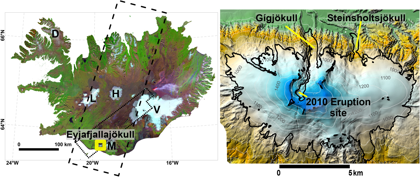
Eyjafjallajökull (Fig. 1) is located ~10 km from the south coast of Iceland, with a climate mainly controlled by the Irminger Current (Björnsson and others, Reference Björnsson2013). Guðmundsson and others (Reference Guðmundsson2011) calculated the geodetic mass balance for 1984–2004 based on contour maps and remote-sensing data, and estimated a higher sensitivity of mass balance to temperature than for other glaciers located further inland (e.g. De Woul and Hock, Reference De Woul and Hock2005; Pálsson and others, Reference Pálsson2012). This is likely explained by the proximity of the ice cap to the coast, with more precipitation and mass-balance amplitude. The April 2010 eruption in Eyjafjallajökull opened a >100 m deep melt channel (Fig. 1), draining northwards and extending close to the glacier margin of the Gígjökull outlet glacier. The estimated ice melt by the eruption was 10–13 × 107 m3 (Oddsson and others, Reference Oddsson2016).
Location map. Left: Mosaic of Landsat 8 images of Iceland. The dashed rectangle shows the footprints of the 1980 KH-9 images. The thin black dotted polygon shows the extent of the 1998 EMISAR DEM (Dall, Reference Dall2003; Magnússon, Reference Magnússon2003), and the thick yellow rectangle shows the location of Eyjafjallajökull. The five largest ice caps, Vatnajökull (V), Langjökull (L), Hofsjökull (H), Mýrdalsjökull (M) and Drangajökull (D) are also shown. Right: Colored shaded relief from a lidar DEM surveyed in August 2010. The black line shows the glacier extent in 2010. The lidar survey took place ~4 months after the 2010 eruption, revealing an open channel of melted ice at the eruption site and along the paths of lava flows extending to the north from the main crater.
3. DATA
The data used in this study are organized into two categories: (1) DEM sources and (2) climate data. Point (1) encompasses three sub-categories: (1) frame stereo imagery, consisting of scanned analog imagery obtained from a camera, (2) pushbroom stereo imagery, i.e. imagery obtained from a pushbroom optical sensor and (3) non-stereo-based DEMs. The last group comprises the lidar DEM from 2010 (Jóhannesson and others, Reference Jóhannesson2013) and an airborne Synthetic Aperture Radar DEM from 1998 (EMISAR; Dall, Reference Dall2003; Magnússon, Reference Magnússon2003), which are further described in online Supplementary material S1.
3.1. DEM sources
3.1.1. Frame stereo imagery
The frame imagery was subdivided into four groups:
(1) 1945–1946 – American Mapping Service (AMS): These surveys, part of the US photoreconnaissance program, consist of a full survey of Iceland in the summers of 1945 and 1946. This series consists of copies of the original films, stored at the National Land Survey of Iceland (Landmælingar Íslands, LMÍ). The cameras had a format of 23 × 23 cm and a focal length of 153 mm. The images from this series typically have a scale of 1: 40 000 (flight altitude of 6700 m a.s.l.).
(2) 1956–1961 – Defense Mapping Agency (DMA): As a continuation of the US photoreconnaissance missions, ~70% of Iceland was resurveyed in the summers of 1956 and 1959 to 1961 except for the eastern part of the country. The data are also a copy of the original films, stored at LMÍ. The cameras used in this survey (format 23 × 23 cm) have basic calibration certificates, including focal length (153 mm) and radial distortion (Spriggs, Reference Spriggs1966).
(3) 1950s–1990s – LMÍ: Photogrammetric campaigns organized by local institutions began to cover selected areas of Iceland in the 1950s, turning into systematic and country-wide surveys in the 1970s. The first campaigns were carried out with small-format images (18 × 18 cm, focal length 115 mm) and were replaced by standard aerial mapping cameras from the 1970s onwards (23 × 23 cm, focal length 153 mm). Original films are available at LMÍ.
(4) 1977–1980 – Hexagon KH-9 Mapping Camera images (KH-9): The declassified satellite photoreconnaissance missions consist of a total of nine satellite missions, spanning 1959–1984, for which most of the data became publicly available between 1992 and 2011 (e.g. Bindschadler and Vornberger, Reference Bindschadler and Vornberger1998; Surazakov and Aizen, Reference Surazakov and Aizen2010). In this study, we use six images from the Hexagon KH-9 mission # 1216, acquired in 1980, crossing Iceland from north to south, including, among other glacierized areas, a complete coverage of Eyjafjallajökull, Mýrdalsjökull, Höfsjökull as well as numerous smaller (size <50 km2) glaciers and ice caps. The images have a format of 23 × 46 cm and a focal length of 305 mm (Surazakov and Aizen, Reference Surazakov and Aizen2010).
The AMS, DMA and LMÍ series were obtained from the National Land Survey of Iceland (http://www.lmi.is), which stores negatives and prints of the aerial surveys carried out from the 1940s to the 1990s. All the data are publicly available upon request, and scanning of the negative films was carried out with a photogrammetric scanner (further details in online Supplementary material S2). The KH-9 satellite frame imagery was obtained from the United States Geological Survey (USGS, https://www.usgs.gov/).
3.1.2. Pushbroom stereo imagery
The pushbroom imagery used can be categorized into three groups:
(1) 2000–present – ASTER: The ASTER satellite has been in operation since 2000 with numerous acquisitions on glaciers thanks to the GLIMS program (Raup and others, Reference Raup2007), and the data collected are publicly available at https://search.earthdata.nasa.gov/. A single stereopair from ASTER, acquired in late summer 2009, was processed to analyze the glacier changes prior to the Eyjafjallajökull 2010 eruption.
(2) 2002–2015 – SPOT5 (©CNES & Airbus D&S): This satellite has been successfully used in numerous surveys of ice masses (e.g. Korona and others, Reference Korona, Berthier, Bernard, Remy and Thouvenot2009). We obtained a stereopair from SPOT5 acquired in October 2004 (Guðmundsson and others, Reference Guðmundsson2011).
(3) 2011–present – Pléiades (©CNES & Airbus D&S): Pléiades stereo images offer the capabilities of creating highly accurate and detailed DEMs in glacierized areas thanks to their geometric and radiometric resolution (Berthier and others, Reference Berthier2014; Belart and others, Reference Belart2017). We use a Pléiades stereopair acquired on 11 August 2014, with an almost complete coverage of the Eyjafjallajökull. Some clouds covered a small portion (~2%) of the southwest margin of the ice cap.
3.2. Climate data
The gridded daily temperature of Iceland, produced by Crochet and Jóhannesson (Reference Crochet and Jóhannesson2011), was used in this study. This dataset consists of 1 × 1 km gridded daily air temperature at 2 m above ground, spanning 1949–2016, deduced by interpolation of weather station observations reduced to sea level with a constant vertical temperature lapse rate of 6.5°C km–1, and adjusted back to the topography with a 1 × 1 km DEM and the same constant vertical lapse rate.
Gridded daily precipitation of Iceland was obtained from two sources: (1) the linear theory model of orographic precipitation (LT-Model, Crochet and others, Reference Crochet2007), available for the period 1958–2007 in 1 × 1 km resolution, and the (2) HARMONIE numerical model (HM-Model, Bengtsson and others, Reference Bengtsson2017; Nawri and others, Reference Nawri, Pálmason, Petersen, Björnsson and Þorsteinsson2017), spanning 1980–2016 with 2.5 × 2.5 km resolution.
The reader is referred to the above studies for details about the climate data and their uncertainties.
4. METHODS
The ‘Methods’ section can be divided into three successive steps: (1) creating maps of elevation difference, (2) calculation of seasonally corrected mass balances and (3) joint analysis of mass balance and climatic data.
4.1. Creating maps of elevation difference
4.1.1. Frame stereo imagery (MicMac)
The frame stereo imagery was processed using the open-source software, MicMac (© National Institute of Geographic and Forestry Information, IGN, France; Pierrot Deseilligny and Clery, Reference Pierrot Deseilligny and Clery2011; Rupnik and others, Reference Rupnik, Daakir and Pierrot Deseilligny2017), to obtain DEMs and orthophoto. The general workflow is explained in Rupnik and others (Reference Rupnik, Daakir and Pierrot Deseilligny2017), and the routines utilized are further described in online Supplementary material S2.
Our pipeline (Fig. 2) started with the scanned frame imagery as input, cropped by the fiducial marks, and 11–20 Ground Control Points (GCPs) manually digitized, extracted from the lidar DEM viewed as a hillshade (e.g. James and others, Reference James, Murray, Barrand and Barr2006; Barrand and others, Reference Barrand, Murray, James, Barr and Mills2009), with an adequate distribution horizontally and vertically outside the ice cap and at nunataks. We measured 65 GCPs for the KH-9 photographs distributed over their overlapping areas with the available lidar data.
Diagram of generic workflow followed. Trapezoids show input data, rectangles indicate processes and ovals indicate outputs.  $\dot{B}_{{\rm EOS}}$ is the glacier-wide mass balance at the end of summer.

The image orientation was solved in two steps: (1) calculating relative orientation from automatic measurements of tie points and SfM, and (2) solving for absolute orientation by robust bundle adjustment using GCPs, in which the camera parameters were also refined. Once the images were oriented, a point cloud was created using semi-global matching and linearly interpolated onto a regular 5 × 5 m grid. A mosaic of orthoimages was also generated.
By using well-distributed GCPs, the likelihood of significant biases in the DEMs relative to the reference DEM was minimized (Magnússon and others, Reference Magnússon, Belart, Pálsson, Ágústsson and Crochet2016). Yet, remaining residual errors in orientation need to be acknowledged, especially in areas far away from GCPs. These errors are spatially-variable, and due to the sensor's geometry, the residual errors can have a significant vertical component. Localized errors in horizontal position can also be expected, particularly in the oldest datasets. We do not attempt to correct horizontal errors, but we acknowledge that relative errors in horizontal positions can affect the obtained vertical errors, studied in the uncertainty analysis (Section 4.1.3).
4.1.2. Pushbroom stereo imagery (ASP)
ASP is a robust, open-source and automated photogrammetric package commonly used for processing pushbroom satellite stereo images (NASA; Shean and others, Reference Shean2016). The pipeline (Fig. 2) used the orbital information from the imagery, generally presented as Rational Polynomial Coefficients (RPCs), and no GCPs were used.
The processing of ASTER and SPOT5 DEMs was performed with an ASP setup slightly modified (Supplement S3) from that of Brun and others (Reference Brun, Berthier, Wagnon, Kääb and Treichler2017), and inspired by Lacroix (Reference Lacroix2016). Pléiades imagery was processed as described in Belart and others (Reference Belart2017).
SPOT5, ASTER and Pléiades DEMs were co-registered to the lidar using the Iterative Closest Point (ICP) algorithm in ASP (Shean and others, Reference Shean2016; Belart and others, Reference Belart2017). The 3D transformation served to refine the orbital information and produce a co-registered orthoimage. Additional details of the processing are explained in online Supplementary material S3.
4.1.3. Correction and uncertainty assessment of the obtained mean elevation change
The difference of DEMs (dDEM) can be affected by spatially-variable errors due to residual errors in the sensor orientation (interior and exterior). This effect can be particularly enhanced in the oldest datasets, e.g. 1945 and 1960, where the camera geometry is not fully constrained (e.g. Magnússon and others, Reference Magnússon, Belart, Pálsson, Ágústsson and Crochet2016).
To correct the spatially-variable errors in the dDEM, we used a modified version of the Sequential Gaussian Simulation (SGSim) described by Magnússon and others (Reference Magnússon, Belart, Pálsson, Ágústsson and Crochet2016). In this study, it is included in an automated pipeline using the command-line interface for the open-source software GSLib (Deutsch, Reference Deutsch1998). The SGSim calculates 1000 realizations of simulated maps (2D grids) of spatially-variable errors for each dDEM within the ice cap, using as input the off-glacier areas of the dDEM and a modeled semivariogram, also constrained by the off-glacier areas of the dDEM.
Each realization simulates the error of the elevation change on each grid node within the ice cap. Averaged over the glacierized area, this results on the simulated error of the glacier-wide the mean elevation change (Table 2). From a probability distribution based on the histogram of the 1000 realizations, we approximated the 95% confidence interval of the glacier-wide mean elevation change.
Unlike Magnússon and others (Reference Magnússon, Belart, Pálsson, Ágústsson and Crochet2016), in this study the dDEMs are not bias corrected based on a single mean of the probability distribution. Instead, we subtracted the derived mean of the 1000 realizations for each individual grid node within the ice cap. This approach results in the same correction for the mean elevation change (Table 2) but also results in more realistic localized corrections for the obtained dDEMs for visualization. Details of the SGSim methodology are described in online Supplementary material S4.
This method takes into account the spatial autocorrelation of the dDEMs, producing a spatially-variable error correction. This results in significantly lower uncertainties in glacier-wide mean elevation change and volume change than proxies based on descriptive statistics (Rolstad and others, Reference Rolstad, Haug and Denby2009; Magnússon and others, Reference Magnússon, Belart, Pálsson, Ágústsson and Crochet2016), such as standard deviation or Normalized Median Absolute Deviation (NMAD, Höhle and Höhle, Reference Höhle and Höhle2009) (Table 2). To verify the robustness of the SGSim, we used the two independent datasets at similar dates in 1960 and 1980, respectively (1960 DMA, 1960 LMÍ, 1980 LMÍ and 1980 KH-9; Table 1), for which we calculated the glacier-wide mean elevation changes compared with the 2010 lidar DEM (considered as a ground truth). We could thus confirm that the glacier-wide mean elevation difference during 1960–2010 and 1980–2010 corrected using SGSim agreed well within the uncertainty estimates using the different datasets, and that the agreement is better than with other, more simplified, bias correction models. The results of these tests are further explained in the online Supplementary Table S1.
Dates, sources and basic information of the datasets. GSD: Ground Sampling Distance (m), approximated for the frame stereo imagery based on the sensor elevation above ground, focal length and scanning resolution
* An intensity map was produced from the lidar pulses, providing an additional mode of visualization of the lidar data for mapping purposes.
Descriptive statistics off-glacier (e.g. Thibert and others, Reference Thibert, Blanc, Vincent and Eckert2008; Höhle and Höhle, Reference Höhle and Höhle2009) and results from SGSim on-glacier (Magnússon and others, Reference Magnússon, Belart, Pálsson, Ágústsson and Crochet2016) from the multiple dDEM combinations, after a slope mask >30° was applied to the dDEMs
4.2. Calculation of seasonally corrected mass balance
The volume changes  ${\rm d}V_{t1}^{t2} {\rm \;} $ for the selected time intervals were calculated from SGSim-corrected maps of elevation change. Since they contained some data gaps (up to 15% of the ice cap area, in the worst case of the 1989 series), a gap interpolation and outlier filtering were also performed, as described in online Supplementary material S5. The glacier-wide geodetic mass balance $\dot{B}$ was calculated with the following equation (Fischer and others, Reference Fischer, Huss and Hoelzle2015; Magnússon and others, Reference Magnússon, Belart, Pálsson, Ágústsson and Crochet2016):
 $$\dot{B}_{t1}^{t2} = \displaystyle{{{\rm d}V_{t1}^{t2} {\rm \;} c} \over {\overline {A_{t{\rm 1}}^{t{\rm 2}}} {\rm \;\ d}t}},$$
where  $\overline {A_{t{\rm 1}}^{t{\rm 2}}} {\rm \;} $ is the average area for the two dates, dt is the time difference, in absolute years, and c is the conversion factor of volume to water equivalent, here chosen as 0.85 ± 0.06 (Huss, Reference Huss2013). This value is recommended over time periods longer than 5 years (Huss, Reference Huss2013), hence we assume twice as large uncertainty ( ± 0.12) for the conversion factor in time periods of 4 and 5 years (1980–1984; 1984–1989; 1989–1994; 1994–1998; 2004–2009; 2010–2014). For the period 2009–2010, a conversion factor of 0.90 ± 0.10 is chosen, assuming the elevation change is mostly due to ice melted by the April 2010 eruption.
The glacier-wide geodetic mass balance was then temporally adjusted to the end of the summer,  $\dot{B}_{{\rm EOS}}$, to facilitate comparison between the different time periods, avoiding the effect of seasonal signals that are particularly strong in a relative sense for short time periods. A volume correction was calculated between the date of each DEM dataset (t1 and t2), and 1 October of the same year (Magnússon and others, Reference Magnússon, Belart, Pálsson, Ágústsson and Crochet2016). For simplicity, the DEMs of 1945, 2004 and 2009 were not shifted seasonally as they were acquired at most 1 week apart from 1 October (Table 1). $\dot{B}_{{\rm EOS}}$ was computed as
 $$\dot{B}_{{\rm EOS}\,{\rm t1}}^{t{\rm 2}} = \displaystyle{{{\rm d}V_{t{\rm 1}}^{t{\rm 2}} -{\rm d}V_{t{\rm 1}}^{{\rm 1\; Oct}} + {\rm d}V_{t{\rm 2}}^{{\rm 1\; Oct}} {\rm \;}} \over {\overline {A_{t{\rm 1}}^{t{\rm 2}}} {\rm \;\ d}t}}c,$$
where  ${\rm d}V_{t{\rm 1}}^{{\rm 1\; Oct}} $ is the volume of the seasonal correction calculated between t1 and 1 October of the same year, and analogously for ${\rm d}V_{t{\rm 2}}^{{\rm 1\; Oct}} $. Eqn (2) neglects the correction of area to 1 October. The seasonal correction integrated over the ice cap was calculated from the climate models of temperature (T) and precipitation (P) as
 $${\rm d}V_{t{\rm DEM}}^{1{\rm \; Oct}} = \mathop \sum \limits_{t{\rm DEM}}^{1{\rm \; Oct}} \mathop \int \limits_{\rm \;} ^{{\rm glacier}} \left\{ {\alpha \displaystyle{{{\rm dd}{\rm f}_{{\rm f}\& {\rm i}}{\rm \;} T_ +} \over {c_{{\rm f}\& {\rm i}}}} + \beta \displaystyle{{{\rm dd}{\rm f}_{\rm s}{\rm \;} T_ +} \over {c_{\rm s}}}-\displaystyle{{P_{(T \lt 1^\circ C)}} \over {c_{\rm s}}}} \right\}(t,x,y){\rm d}A,$$
where  ${\rm dd}{\rm f}_{{\rm f}\& {\rm i}}$ is a degree-day factor of firn and ice of 6.5 ± 1.5 mm w.e. °C–1 (Magnússon and others, Reference Magnússon, Belart, Pálsson, Ágústsson and Crochet2016), ddfs is a degree-day factor of snow of 3.5 ± 1.5 mm w.e. °C–1 (online Supplementary material S6), $c_{{\rm f}\& {\rm i}}$ is the average conversion factor of firn and ice to water, 0.75 ± 0.1 and c s is the conversion factor of snow to water of 0.5 ± 0.1.α and β are binary switches; α = 1 and β = 0, meaning that the glacier surface at the location analyzed contains firn or ice, until
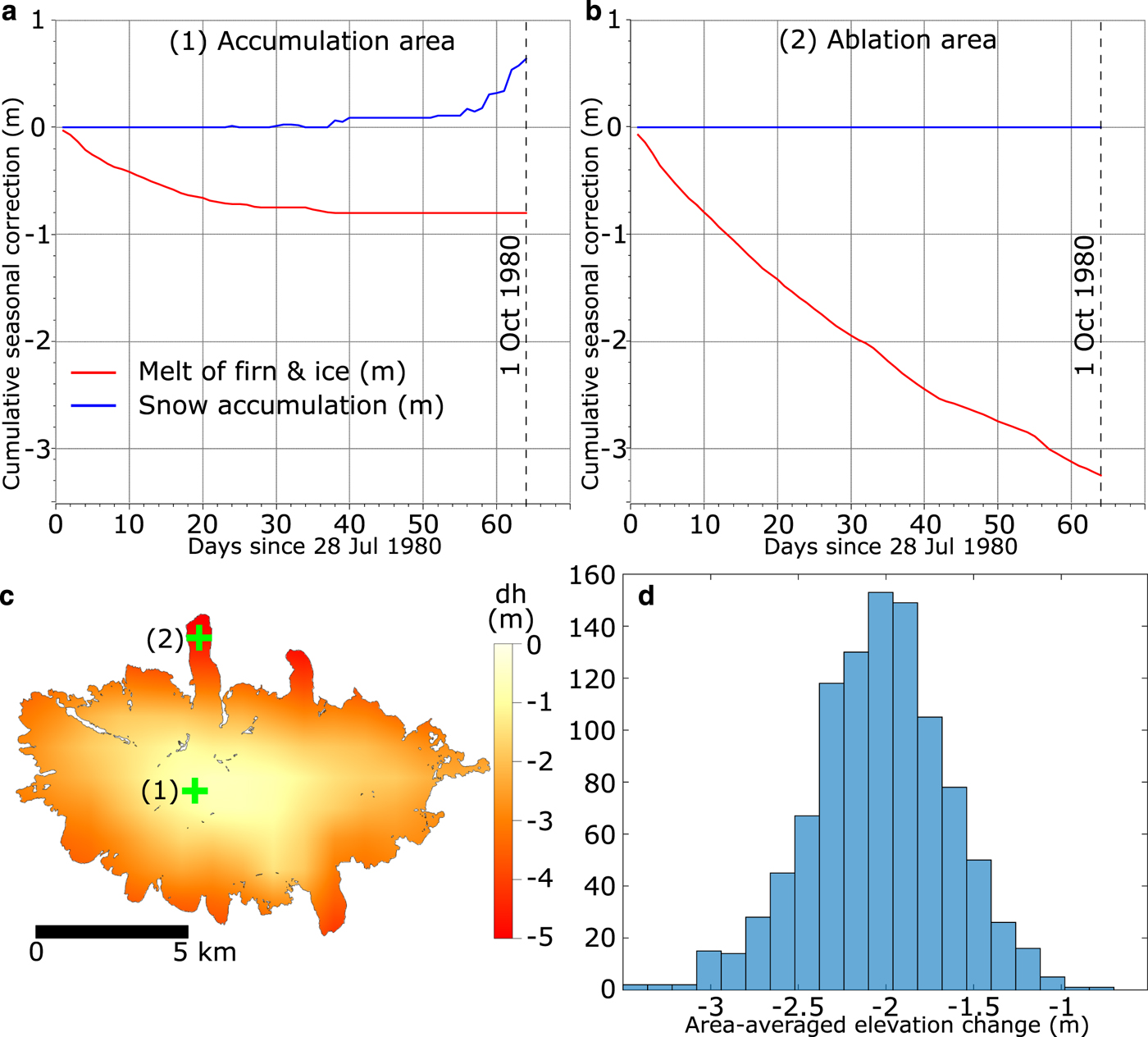
  $P_{(T \lt 1^\circ C)} \lt 0$, when they switch to α = 0 and β = 1, meaning that new snow is present at the location, changing the ddf and conversion factor. If the new snow is completely melted, the switches turn back to α = 0 and β = 1 as firn and ice reappear on the glacier surface (Fig. 3). The gridded temperature was used to calculate the positive degree-days, T +, and to set the 1°C threshold between rain and snow in precipitation (e.g. Jóhannesson and others, Reference Jóhannesson, Sigurðsson, Laumann and Kennett1995). The HM-Model was utilized to infer P for the period 1980–2014 and the seasonal corrections involving the 1960 datasets were computed with the LT-Model after scaling it toward the HM-Model by linearly fitting summer precipitation in the overlapping time period (1980–2006). The gridded climate data were bilinearly resampled to 20 × 20 m grids to adequately crop the coarse model results to the glacier outline.
(a, b) One iteration of calculated cumulative seasonal correction, at two grid locations (1) and (2), between 28 July 1980 and 1 October 1980 (the longest seasonal correction). (c) Total seasonal correction for the same iteration (cumulative melt minus cumulative snow accumulation). Green crosses indicate location of the profiles in (a) and (b). (d) A histogram of 1000 realizations of the seasonal correction (averaged over the whole ice cap) from bootstrapping.
This methodology ignores changes in ice-surface elevation caused by vertical ice motion, which is on the same order as the seasonal mass balance. This does not matter for glacier-wide calculations as the integral of the vertical ice-surface velocity is zero over whole ice flow basins by continuity (e.g. Cuffey and Paterson, Reference Cuffey and Paterson2010).
The seasonal correction from Eqn (3) was calculated by bootstrapping, performing 1000 realizations of the correction and adding random Gaussian errors on each iteration to the variables  ${\rm dd}{\rm f}_{{\rm f}\& {\rm i}}$, ddfs, $c_{{\rm f}\& {\rm i}}$, c s, T and P. A summary of parameters and uncertainties is described in the online Supplementary material S6. The errors added to T and P were applied as offsets, up to ±0.5°C (T) and ±50 mm (P) to the entire climatic data on Eyjafjallajökull, as random errors at individual grid points would cancel each other out in the bootstrapping method and spatially widespread offsets are more likely to occur (Nawri and others, Reference Nawri, Pálmason, Petersen, Björnsson and Þorsteinsson2017). From the histogram of the 1000 realizations, we extracted the median value of ${\rm d}V_{t{\rm DEM}}^{1\; {\rm Oct}} $ with the 95% confidence interval for each date of survey (Fig. 3). Results of this correction are summarized in online supplementary Table S3.
The uncertainties of  $\dot{B}$ and $\dot{B}_{{\rm EOS}}$, $\delta \dot{B}_{t1}^{t2} $ and $\delta \dot{B}_{{\rm EOS}\,t1}^{t2} $ were calculated by the addition in quadrature of the partial derivative of each variable multiplied by its uncertainty, assuming that the variables of Eqns (1) and (2) were uncorrelated and had uncertainties following normal distributions (Fischer and others, Reference Fischer, Huss and Hoelzle2015; Magnússon and others, Reference Magnússon, Belart, Pálsson, Ágústsson and Crochet2016).
The glacierized areas were always digitized by the same operator and using the same criteria of definition of the ice cap boundaries. Uncertainties in the area were neglected; given the size of Eyjafjallajökull, the maximum area uncertainty was assumed of 5%, as digitized from the coarsest resolution (ASTER) dataset (Raup and others, Reference Raup, Kargel, Leonard, Bishop, Kääb and Raup2014). This would only lead to <0.01 m w.e. a–1 increase in uncertainty of the geodetic mass balance. Thus,  $\delta \dot{B}_{t1}^{t2} $ and $\delta \dot{B}_{{\rm EOS}\,t1}^{t2} $ were calculated as
 $$\delta \dot{B}_{t1}^{t2} = \displaystyle{1 \over {\overline {A_{t1}^{t2}} {\rm d}t}}\sqrt {{\lpar {c\delta V_{t1}^{t2} {\rm \;}} \rpar }^2 + {\lpar {{\rm d}V_{t1}^{t2} \delta c} \rpar }^2} $$
 $$\delta \dot{B}_{{\rm EOS}\,t1}^{t2} = \displaystyle{1 \over {\overline {A_{t1}^{t2} } {\rm d}t}}\sqrt {\matrix{{\left( {c\delta V_{t1}^{t2} {\rm \; }} \right)}^2 + {\left( {c\delta V_{t1}^{1\; {\rm Oct}} } \right)}^2 + {\left( {c\delta V_{t2}^{1{\rm \; Oct}} } \right)}^2 \cr + {\left( {\left( {{\rm d}V_{t1}^{t2} -{\rm d}V_{t1}^{1{\rm \; }Oct} + {\rm d}V_{t2}^{1{\rm \; Oct}} } \right)\delta c} \right)}^2}} ,$$
where  $\delta V_{t1}^{t2} \delta V_{t1}^{1\; {\rm Oct}} $, $\delta V_{t2}^{1\; {\rm Oct}} $ and δc are the uncertainties of $V_{t1}^{t2} V_{t2}^{1{\rm \; Oct}}, \; V_{t2}^{1\; {\rm Oct}} $ and c, respectively.
4.3. Joint analysis of mass balance and climatic records
The calculated  ${\dot B}_{{\rm EOS}}$ overlaps in time with the climatic records for the period 1960–2014. With these data we calculated the linear regression relating mass balance and climate forcing, which also allowed retrieving the static mass-balance sensitivity to changes in climatic variables (De Woul and Hock, Reference De Woul and Hock2005; Ohmura, Reference Ohmura2011; Sakai and Fujita, Reference Sakai and Fujita2017). The time span of our observations is long enough to be affected by dynamic adjustments of glacier geometry (Huss and others, Reference Huss, Hock, Bauder and Funk2012). We thus assume that the annual, reference-surface mass balance (Elsberg and others, Reference Elsberg, Harrison, Echelmeyer and Krimmel2001; Harrison and others, Reference Harrison, Elsberg, Echelmeyer and Krimmel2001) can be described linearly as a function of the summer temperature, Ts, and winter precipitation, Pw (e.g. Oerlemans and Reichert, Reference Oerlemans and Reichert2000; De Woul and Hock, Reference De Woul and Hock2005; Schuler and others, Reference Schuler2005).
 $${\dot B}_{{\rm EOS}} + b_{\rm g}\Delta V + b_{\rm a}\Delta A = \varphi T{\rm s} + \omega P{\rm w} + k,$$
where b g and b a are the effective balance-rate gradient and balance rate at the terminus, respectively, and ΔV and ΔA are the changes in volume and area between a reference date and the intermediate date of each time period, respectively.
The static sensitivity of mass balance to 1°C warming in summer temperature,  $\partial {\dot B}/\partial T{\rm s}$, is represented by φ, and analogously, $\partial {\dot B}/\partial P{\rm w} = \omega $, which yields the sensitivity of mass balance to changes in winter precipitation. The parameter k represents a residual term due to any non-linear effect of the above variables as well as the contribution of other variables affecting the mass balance not accounted for (Oerlemans and Reichert, Reference Oerlemans and Reichert2000). The ‘Discussion’ section explains several non-climatic processes that can alter Eqn (6).
With the gridded climatic records, we calculated summer temperature and winter precipitation for each year at the Equilibrium Line Altitude (ELA, De Woul and Hock, Reference De Woul and Hock2005) of Eyjafjallajökull. We defined the hydrological year as 1 October to 30 September, with the beginning of summer on 20 May (Magnússon and others, Reference Magnússon, Belart, Pálsson, Ágústsson and Crochet2016; Belart and others, Reference Belart2017). The results were averaged to match the time periods of the geodetic mass balance from 1960 to 2014. We excluded the intervals 2009–2010 and 2010–2014 in the analysis, since they were strongly affected by the April 2010 volcanic eruption. The winter precipitation 1960–1980 was calculated from the LT-Model after linearly adjusting it to the HM-Model using winter precipitation in the overlapping years (1980–2006). For the periods 1960–1980 and 1980–1984, we selected the geodetic results extracted from the KH-9 DEM, as the required seasonal correction was smaller.
The precipitation was normalized (Oerlemans and Reichert, Reference Oerlemans and Reichert2000), dividing it by the average winter precipitation during 1960–2014: 5220 mm. This value is similar to the rates of winter accumulation measured on the neighboring Mýrdalsjökull ice cap (Ágústsson and others, Reference Ágústsson, Hannesdóttir, Thorsteinsson, Pálsson and Oddsson2013). Sensitivity to a 10% winter precipitation increase was therefore calculated as 10% of ω (e.g. Oerlemans and Reichert, Reference Oerlemans and Reichert2000; Schuler and others, Reference Schuler2005).
Altogether we obtained seven independent equations that were solved by weighted least-squares fit. We performed the adjustment based on two scenarios: (1) fixing b g = 0.01 a–1 and b a = −5 ma–1 as a first estimate based on the literature (Harrison and others, Reference Harrison, Elsberg, Echelmeyer and Krimmel2001) and from the geodetic records of Eyjafjallajökull and solving for three unknowns (φ, ω, k); and (2) considering that ΔV and ΔA are linearly dependent for the analyzed time periods (R 2 = 0.97, N = 7), Eqn (6) can be simplified to
 $${\dot B}_{{\rm EOS}} = \varphi T{\rm s} + \omega P{\rm w} + \gamma \Delta A + k,$$
where γ includes both terms b g and b a and allows solving the least-square fit with four unknowns (φ, ω, γ, k). Both scenarios yielded highly similar results. We did not attempt to solve the terms b g and b a, as additional unknowns in the least-square fit since the system may become unstable, due to limited amount of observations and high correlation between terms.
Finally, using Eqn (7) with the solved parameters, we computed the annual mass balance from 1958 to 2014 using the annual winter precipitation, summer temperature and glacier area, the latter assumed to change at the same annual rate between each two datasets.
Alternative equations to estimate mass balance from climatic variables were tested but did not yield a better fit than using Eqn (7). This included (a) using annual temperature and precipitation (Guðmundsson and others, Reference Guðmundsson2011; Pálsson and others, Reference Pálsson2012) and (b) using the number of positive degree-days.
5. RESULTS
5.1. Elevation changes and their uncertainties
The SGSim-correction applied to the dDEMs yielded uncertainties of sub-meter to a meter (Table 2) in the glacier-wide elevation difference. Other proxies to assess bias and uncertainties of the dDEM that were based on descriptive statistics, such as the median and NMAD off-glacier, led to substantially different biases and larger uncertainties (Table 2 and Table S1), as already observed by Magnússon and others (Reference Magnússon, Belart, Pálsson, Ágústsson and Crochet2016) and Rolstad and others (Reference Rolstad, Haug and Denby2009).
For the years 1960 and 1980, two independent surveys were carried out on Eyjafjallajökull. This provides a unique opportunity to compare the results of the descriptive statistics and SGSim. When using the SGSim-correction for two datasets with close dates of survey, 1960 DMA and 1960 LMÍ series (Table 1), the glacier-wide mean elevation change during 1960–2010 is − 13.83 ± 0.31 and − 13.38 ± 0.41 m, respectively (Table 1). The remaining difference can be attributed to − 0.36 ± 0.14 m of melting between datasets, calculated from the seasonal correction (Section 4.2). Similarly, the glacier-wide mean elevation change during 1980–2010 is − 20.13 ± 0.41 m (LMÍ dataset) and − 19.35 ± 0.99 m (KH-9 dataset). In this case, the seasonal effect is larger, − 1.43 ± 0.44 m, also likely explaining most of the observed difference. Much larger mismatches of glacier-wide mean elevation difference were found when applying the median correction based on the dDEM's off-glacier areas, up to 3.4 m difference (both series of 1960–2010) and up to 3.5 m difference (both series 1980–2010), which further diverge when applying seasonal correction.
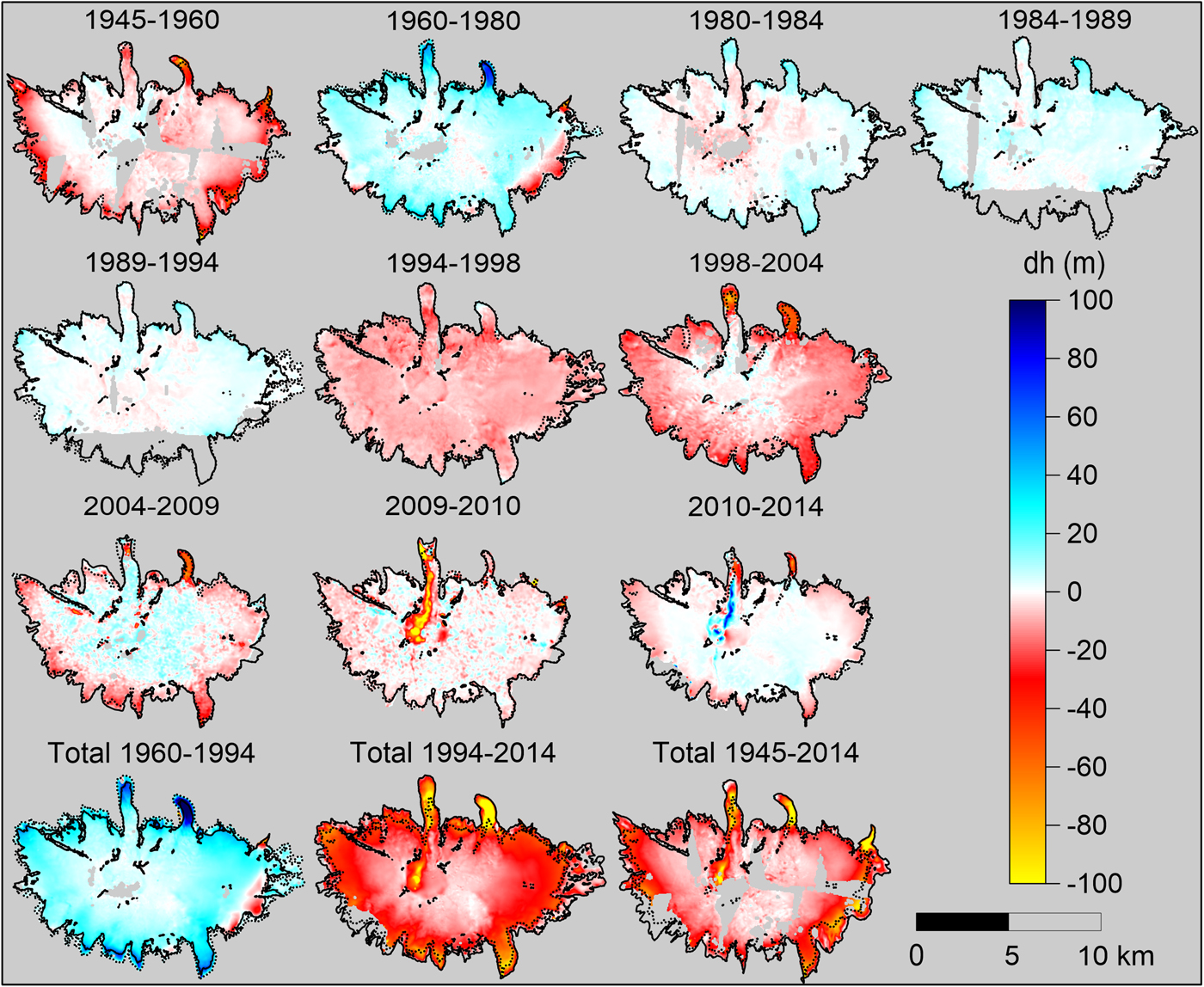
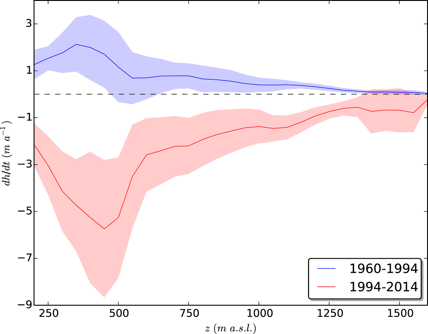
The time series of elevation changes reveal strong fluctuations in the elevation of the ice cap through recent decades, showing overall thinning in 1945–1960 and 1994–2014, and thickening in 1960–1994 (Figs 4 and 5). The rates of elevation change in 1960–1994 (thickening) and 1994–2014 (thinning) show a mirrored pattern in the rate of elevation change as a function of altitude (Fig. 5). Glacier-wide mean elevation change is 14 m for 1960–1994 and −27 m for 1994–2014. The glacier catchments on the north side (Gígjökull and Steinsholtsjökull, Fig. 1) contain the fastest-changing outlets, thickening up to 130 m in 1960–1994 and thinning up to 200 m in 1994–2014 near their respective termini.
Time series of elevation changes of Eyjafjallajökull. The dDEMs were plotted after applying the SGSim and seasonal corrections, hence all dates are relative to 1 October. Red and yellow colors indicate lowering, and cyan and blue indicate thickening. A continuous black polygon and a dashed black polygon indicate the ice cap extent and nunataks at the start and end of the analyzed time period, respectively. The three bottom images show the total elevation changes during multi-decadal time periods, 1960–1994 (mass gain), 1994–2014 (mass loss) and 1945–2014 (longest time interval).
Mean rate of elevation change extracted for 50 m elevation bands (solid lines) and the corresponding standard deviation (filled areas) for the two time periods with the most extreme changes: 1960–1994 (blue) and 1994–2014 (red).
The changes in the most recent periods, 2009–2010 and 2010–2014, are affected by the April 2010 Eyjafjallajökull eruption. A maximum thinning of 180 m is observed in 2009–2010, due to the subglacial melting along the lava paths of the 2010 eruption, and filling of the opened channel is observed in 2010–2014 as a result of the inflow of ice in the depression (e.g. Aðalgeirsdóttir and others, Reference Aðalgeirsdóttir, Guðmundsson and Björnsson2000), leading to a maximum thickening of 100 m in 2010–2014 (Fig. 4).
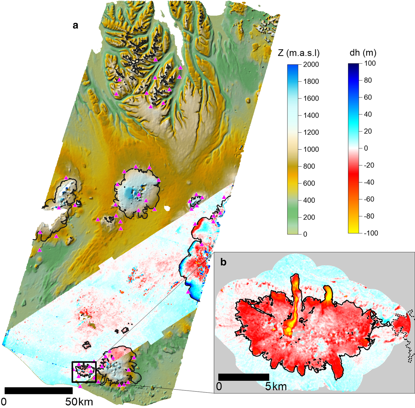
The DEM and orthoimage created from the declassified KH-9 imagery cover approximately one-third of Iceland and about one-third of the glacierized areas (~3400 km2) of the country (Fig. 6). From the comparison with the 2010 lidar, the SGSim-corrected glacier-wide elevation change has an uncertainty of 1 m at the 95% confidence level (online supplementary Table S1). The KH-9 DEM and EMISAR DEMs have a large overlap, allowing the comparison between the datasets and analysis of large-scale elevation changes, not only for Eyjafjallajökull. Results show a good fit between the KH-9 DEM and EMISAR, with a median elevation difference of 2.08 m and NMAD of 5.73 m in all unchanged areas, including areas far away (>50 km) from the GCPs (Fig. 6). These statistics are partially affected by the errors of the EMISAR DEM, which has a relative accuracy of 1–2 m (Magnússon, Reference Magnússon2003; Guðmundsson and others, Reference Guðmundsson2011) as well as errors related to the different resolution of the grids compared. This comparison also reveals clear signals of glacier changes during 1980–1998, specifically mass loss of Eyjafjallajökull and Mýrdalsjökull, and advancement of the several surging outlet glaciers in west Vatnajökull (Björnsson and others, Reference Björnsson, Pálsson, Sigurðsson and Flowers2003).
Results from 1980 KH-9 processing. (a) KH-9 DEM from 22 August 1980 in a color hillshade, overlaid with the difference of elevation between the KH-9 DEM and the EMISAR DEM (1998). Red color indicates lowering, and blue color indicates an increase in elevation. Triangles show the GCPs used for the processing of the KH-9 DEM, located where lidar data were available. The outlines of glacierized areas are shown with black lines, extracted from the GLIMS glacier database (Raup and others, Reference Raup2007). Note the thickening at the margin of the southwest outlets from Vatnajökull ice cap, which surged between 1992 and 1994 (Björnsson and others, Reference Björnsson2003). (b) Difference in elevation between the KH-9 DEM (1980) and the lidar DEM (2010), together with elevation differences within a 2 km buffer from the glacier outline. The greatest lowering is due to the April 2010 Eyjafjallajökull eruption and the melting of Steinsholtsjökull (northwest). Dashed lines indicate the neighbor ice cap, Mýrdalsjökull.
5.2. Geodetic mass balance
The geodetic records yield a negative mass balance of  ${\dot B}_{{\rm EOS}\,1945}^{2014} = -0.27 \pm 0.03\,{\rm m\ w}{\rm. e}{\rm.} {\rm a}^{{\rm \ndash 1}}$ for the entire study period, reaching a maximum of ${\dot B}_{{\rm EOS}\,1984}^{1989} = 0.77 \pm 0.19\,{\rm m\ w}{\rm. e}{\rm.} {\rm a}^{{\rm \ndash 1}}$ and a minimum of ${\dot B}_{{\rm EOS}\,1994}^{1998} = -1.94 \pm&InLnBrk; 0.34\,{\rm m\ w}{\rm. e}{\rm.} {\rm a}^{{\rm \ndash 1}}$. During the period 2009–2010, which includes the Eyjafjallajökull eruption, the mass loss was ${\dot B}_{2009}^{2010} = -3.39 \pm 0.43\,{\rm m\ w}{\rm. e}{\rm.} {\rm a}^{{\rm \ndash 1}}$ (without seasonal correction, further described in the ‘Discussion’ section). Detailed results of the mass balance for each time interval are provided in Table 3.
Glacier-wide geodetic mass balance of Eyjafjallajökull with and without seasonal correction
*  ${\dot B}_{{\rm EOS}}$ obtained after applying seasonal correction on the 2010 dataset (the insulation effect from the tephra is not taken into account).
†  ${\dot B}_{{\rm EOS}}$ calculated excluding the seasonal correction of the 2010 dataset (assuming the tephra layer insulated the ice cap during summer 2010).
There are differences up to 0.4 m w.e. a–1 between uncorrected and seasonally-corrected geodetic mass balances for periods as short as 4–6 years, but the difference becomes negligible for long periods (⩾20 years, Table 3). The seasonal correction is particularly high when using the LMÍ datasets from the 1980s due to seasonal variations in acquisition dates (Table 1). The largest seasonal correction was − 1.98 ± 0.69 m (glacier-wide lowering) for the LMÍ DEM of 28 July 1980, since it was acquired 2 months before the end of the summer, whereas − 0.56 ± 0.40 m was estimated between 22 August 1980 (KH-9) and 30 September 1980. The seasonal corrections for each date of survey are listed in online Supplementary material S6 and Table S2.
5.3. Correlation between climatic variables and geodetic mass balance
The time series of summer temperature at the ELA (1200–1300 m a.s.l.) and its average over the time periods of the geodetic mass balance reveal a clear cooling during the early 1980s, reaching a minimum of  $T{\rm s}_{1980}^{1984} = 1.9^\circ {\rm C}$, averaged. Temperatures gradually increased to $T{\rm s}_{1998}^{2004} = 3.3^\circ {\rm C}$, and remained high with little change until 2014 (Fig. 7).
(a) Inferred summer temperature at the ELA during 1948–2015 (dashed lines) and averages over the time periods of the geodetic mass balance (solid lines). (b) Normalized winter precipitation at ELA (winter precipitation divided by 1960–2014 average), both annual (dashed line) and averaged over the geodetic mass-balance periods (solid lines). The period 1958–1979 was calculated from the scaled LT-Model (Section 4.3), and the period 1980–2015 was extracted from the HM-Model. (c) Black points indicate the area measured at each year of survey. (d) Comparison between observed  ${\dot B}_{{\rm EOS}}$ (cyan lines) and mass balance deduced from linear regression (Eqn 7) (black lines). The plotted mass balance and area involving the 1980 dataset is calculated using the KH-9 series because it is closer to the end of the summer. All dates are fixed to the hydrological year starting on 1 October. The mass balance 2009–2010 was heavily affected by the volcanic eruption and is therefore not included in the mass balance obtained from the linear regression.
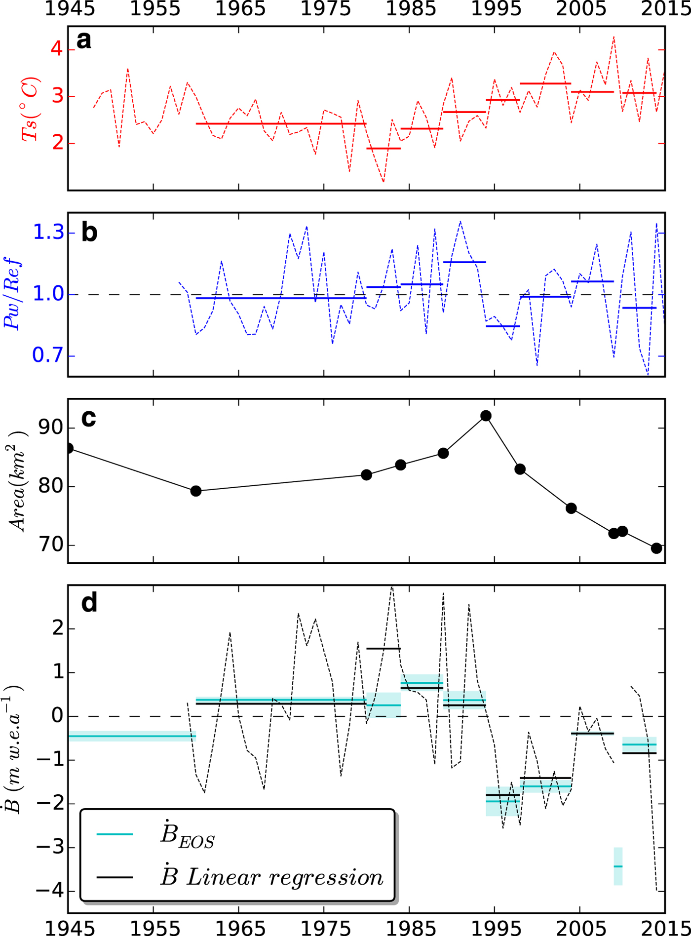
On the other hand, the winter precipitation shows an increase with a maximum of  $P{\rm w}_{1989}^{1994} /{\rm ref} = 1.15$. This is followed by a drop and a minimum of $P{\rm w}_{1994}^{1998} /{\rm ref} = 0.85.$ The last three time periods are close to average and have a high annual variability (Fig. 7).
Results from the linear fit of seasonally corrected, reference-surface geodetic mass balance and climate records yield a static mass-balance sensitivity to 1°C warming in summer temperature and 10% increase in winter precipitation of − 2.08 ± 0.45 m w.e.a–1K–1 and 0.51 ± 0.25 m w.e.a–1 (10%)–1, respectively. The mass balance obtained from linear regression compared with the observed mass balance yielded a coefficient of determination R 2 = 0.81 (N = 7). The mean absolute residual is 0.28 m w.e. a–1, with highest residual of 1.30 m w.e. a–1 for the period 1980–84 (Fig. 7). The annual mass balance obtained from linear regression yields an interannual variability of (SD = 1.57 m w.e. a–1, N = 56).
6. DISCUSSION
6.1. Remote-sensing and open-source alternatives: MicMac, ASP and GSLib
The pipeline of processing stereoscopic data (aerial, spaceborne, frame and pushbroom) and assessing uncertainties was carried out in a semi-automated workflow. Manual steps in the workflow are: (1) measurement of fiducial marks in the frame imagery, (2) measurements of GCPs, (3) digitization of glacier outlines, (4) manual mask of unfiltered artifacts and (5) fitting of a semivariogram model.
Many studies have used photogrammetry and SfM for DEM generation for glaciers with historical aerial photographs generally using commercial software (e.g. Barrand and others, Reference Barrand, Murray, James, Barr and Mills2009; Mölg and Bolch, Reference Mölg and Bolch2017; Fieber and others, Reference Fieber2018). Here the entire processing was carried out using only open-source software (MicMac). The obtained uncertainties of elevation changes are similar to previous studies using commercial software, such as ERDAS Imagine for frame stereo imagery processing (e.g. Magnússon and others, Reference Magnússon, Belart, Pálsson, Ágústsson and Crochet2016) or PCI Geomatica for pushbroom stereo imagery processing (Berthier and others, Reference Berthier2014). The use of semi-global matching in point cloud generation produces an excellent level of detail and limited gaps in DEMs, even in snow areas with low contrast. This illustrates that robust scientific research can be carried out using open-source alternatives. In addition, most input data for our study are open access (see ‘Data availability’ section below). The semi-automated pipelines and open data provide important tools that can be used in future work, given the amount of historical aerial photographs available in Iceland and elsewhere.
This study further supports the need for robust geostatistics to assess uncertainties of volume changes deduced from DEM difference. The bias correction and uncertainties are substantially different than the ones obtained by descriptive statistics (Table 2), as previously shown by Rolstad and others (Reference Rolstad, Haug and Denby2009) and Magnússon and others (Reference Magnússon, Belart, Pálsson, Ágústsson and Crochet2016). The tests using two surveys conducted close in time both in 1960 and 1980 (online supplementary Table S1) show excellent agreement of glacier-wide mean elevation changes between each dataset and the 2010 lidar DEM using the SGSim-correction. The difference between glacier-wide elevation changes when utilizing different datasets is <1 and <2 m for 1960–2010 and 1980–2010, respectively, which is to a large degree explained by the seasonal elevation change between the respective surveys.
Other tests for glacier-wide bias correction and uncertainty estimates, like the median and NMAD of the off-glacier areas or the median and NMAD of the off-glacier areas with a 1 km buffer from the ice cap boundary, led to higher discrepancies in the comparisons of the glacier-wide elevation change 1960–2010 using the twin datasets of 1960, and analogously for the twin comparisons of 1980–2010. While the three methods applied to correct the glacier-wide mean elevation change agreed within their error bars, the error bars of the SGSim were substantially smaller. This further supports that higher level of information can be extracted from geodetic records when applying SGSim (Magnússon and others, Reference Magnússon, Belart, Pálsson, Ágústsson and Crochet2016).
Our work exploits Hexagon KH-9 Mapping Camera stereo imagery, generating a DEM of about one-third of Iceland and covering ~3400 km2 of the following ice masses: Mýrdalsjökull, Hofsjökull, east Langjökull, west Vatnajökull and numerous glaciers with an area <50 km2 (Fig. 5). The comparison with lidar in ice- and snow-free areas yields a NMAD = 4.07 m (proxy for DEM precision) on slopes <30°, and its uncertainty derived from the SGSim-corrected glacier-wide elevation change compared with lidar was 1 m on Eyjafjallajökull (95% confidence level, online supplementary Table S1). This strengthens the potential of these datasets in geodetic mass-balance studies.
A comparison with an independent DEM from the source of GCPs (EMISAR DEM) shows limited distortion of the DEM (NMAD = 5.73 m), including areas far away from GCPs. It also reveals the changes in Eyjafjallakökull, Tindfjallajökull, Torfajökull and the western side of Vatnajökull between 1980 and 1998 (Fig. 6), in particular the advances of some outlets of west Vatnajökull due to their surges in the early 1990s (Björnsson and others, Reference Björnsson, Pálsson, Sigurðsson and Flowers2003). We did not run SGSim between KH-9 and EMISAR DEMs, since no further analysis of a particular area of interest was carried out based on this comparison. The KH-9 spy satellites imaged the entire country in 1977–1980, and previous spy satellite missions imaged large areas of the country since the 1960s (data not scanned, USGS, https://www.usgs.gov/), making these datasets useful for expanding knowledge of the state of Icelandic glaciers at a time of lower temperatures and higher precipitation than at present (Fig. 7).
The time series of elevation differences were completed using spaceborne, pushbroom-based stereo imagery from the last two decades. ASTER offers high potential for producing a series of elevation differences from 2000 to present (Nuimura and others, Reference Nuimura, Fujita, Yamaguchi and Sharma2012; Willis and others, Reference Willis, Melkonian, Pritchard and Rivera2012; Berthier and others, Reference Berthier, Cabot, Vincent and Six2016; Brun and others, Reference Brun, Berthier, Wagnon, Kääb and Treichler2017) and enabled constraining the signal of ice–volcano interaction to the period 2009–2010. SPOT5 provided a DEM observation in 2004, resulting on larger temporal resolution for 2000–2010. Both ASTER and SPOT5 DEMs were processed with open-source software, and the uncertainty obtained was comparable to or better than other studies using similar datasets (e.g. Korona and others, Reference Korona, Berthier, Bernard, Remy and Thouvenot2009; Berthier and others, Reference Berthier, Cabot, Vincent and Six2016).
Our methodology relies on an accurate and high-resolution DEM as a source of GCPs for the frame imagery and for co-registration for the pushbroom imagery. Alternatively to the lidar DEM used here, other data sources could be used, such as a Pléiades-based data (Papasodoro and others, Reference Papasodoro, Berthier, Royer, Zdanowicz and Langlois2015) or WorldView-based data (Fieber and others, Reference Fieber2018). The relative precision of Pléiades- and WorldView-based DEMs is <0.5 m (slopes <10°) and overall <1 m (e.g. Berthier and others, Reference Berthier2014; Shean and others, Reference Shean2016; Belart and others, Reference Belart2017), often close to the precision of lidar (e.g. Jóhannesson and others, Reference Jóhannesson, Björnsson, Pálsson, Sigurðsson and Þorsteinsson2011). The absolute accuracy of these DEMs is affected by uniform horizontal and vertical biases on the order of meters or a few meters and to some degree by tilts leading to vertical biases on the same order, but these cancel out in the calculation of elevation changes if GCPs are based on the same Pléiades- and WorldView-based DEMs. Both data sources are of relatively easy access to the research community; e.g. WorldView DEMs are freely available for latitudes >60°N via ArcticDEM (Porter and others, Reference Porter2018).
6.2. Area, elevation and mass-balance changes in Eyjafjallajökull
The ice cap retreated and thinned in 1945–1960, advanced and thickened in 1960–1994 and retreated and thinned again in 1994–2014. In situ observations of front variations from the Icelandic Glaciological Society (http://spordakost.jorfi.is/) indicate that the outlet Gígjökull started to advance between 1971 and 1979 (Sigurðsson, Reference Sigurðsson1998). The northern outlets show much more rapid front changes than the southern outlets, suggesting higher ice motion in the northern ice catchments vs the southern catchments. This also explains why during 1960–1980 the northern outlets were advancing and thickening while the southeast and southwest margins were still retreating (Fig. 4). There is a lag between the maximum geodetic mass balance in 1984–1989 and the area maximum, reached in 1994 (Fig. 7), which is due to the delayed response of the glacier to the climatic forcing (e.g. Bahr and others, Reference Bahr, Pfeffer, Sassolas and Meier1998).
Our study underlines the importance of seasonal corrections in the interpretation of records of geodetic mass balance, in particular for maritime glaciers with a high mass-balance amplitude (Ágústsson and others, Reference Ágústsson, Hannesdóttir, Thorsteinsson, Pálsson and Oddsson2013; Magnússon and others, Reference Magnússon, Belart, Pálsson, Ágústsson and Crochet2016; Belart and others, Reference Belart2017). Without seasonal corrections, the geodetic mass balances can be misleading over short time periods, for instance in the 1980s when the surveys were conducted during various times in the season (Table 1). However, the seasonal corrections are negligible in long (⩾20 years) time periods. Our approach to correct seasonal volume changes refined the degree-day model of Magnússon and others (Reference Magnússon, Belart, Pálsson, Ágústsson and Crochet2016) by accounting for snowfall and snow melt at high elevation, and used bootstrapping to infer the uncertainty, which is generally 30–50% of the correction (Fig. 3). The uncertainty increases with snow correction (generally in late summer) due to the uncertainty in the snow parameters, i.e. the temperature threshold between rain and snow, ddf and snow density.
The seasonal correction applied to the 2010 dataset was, however, significantly affected by the 2010 volcanic eruption. The ddf does not take into consideration the tephra deposited on the surface of the ice cap. The maps of tephra thickness indicate >2 cm of tephra around Eyjafjallajökull and up to 1 m at locations close to the crater (Guðmundsson and others, Reference Guðmundsson2012). This likely enhanced the melt locally at the lowest elevations, but insulated the majority of the ice cap during summer 2010 (Dragosics and others, Reference Dragosics2016). The seasonal correction presented for August–October 2010 would likely be too negative, leading to an overestimation of the melting during this period.
We do not account for elevation change and subsequent volume change due to firn and fresh snow densification in the seasonal corrections as this can only lead to a minor volume correction. If we assume similar rates of firn and fresh snow densification as calculated for Drangajökull ice cap, northwest Iceland (Belart and others, Reference Belart2017), this would lead to a glacier-wide correction of ~0.07 m, or 3% of the calculated seasonal correction for the the 1980 LMÍ dataset (the largest seasonal correction), well within the uncertainty estimates.
The obtained geodetic mass balances agree within the error bars with the results from Guðmundsson and others (Reference Guðmundsson2011) for Eyjafjallajökull. In comparison to Drangajökull ice cap (northwest Iceland), the geodetic mass balance 1945–2014 follows a similar trend to that calculated for 1946–2011 by Magnússon and others (Reference Magnússon, Belart, Pálsson, Ágústsson and Crochet2016). However, Eyjafjallajökull reveals larger decadal variations, which is consistent with its proximity to the persistent paths of the North Atlantic low-pressure system, with high precipitation rates, and the warm sea surface temperatures from the Irminger ocean current that largely controls the temperatures over the ice cap. Drangajökull on the other hand is likely affected by the cold East Greenland current (Björnsson and others, Reference Björnsson2013).
6.3. Relation between glacier and climate
In our study period, the geodetic mass balance was higher at times with lower temperatures and higher precipitation, and vice versa (Fig. 7). Previous studies have analyzed mass-balance sensitivity in relation to temperature, by using geodetic mass balance and records from nearby weather stations (Guðmundsson and others, Reference Guðmundsson2011; Pálsson and others, Reference Pálsson2012). These studies, however, found a high variability in the results depending on which weather station was used. Other limitations were the use of few time periods and the fact that they did not include sensitivity to precipitation. The long-term records of gridded climate data (Crochet and others, Reference Crochet2007; Crochet and Jóhannesson, Reference Crochet and Jóhannesson2011; Nawri and others, Reference Nawri, Pálmason, Petersen, Björnsson and Þorsteinsson2017) and geodetic mass balance allow more in-depth study of the ice cap's response to climate variations.
The link between climate and mass balance needs to account for glacier adjustment to different climates, especially if the mass-balance records span long time periods in comparison to the relatively short response time of the glacier. This is accounted for by calculating reference-surface mass balance (Elsberg and others, Reference Elsberg, Harrison, Echelmeyer and Krimmel2001; Harrison and others, Reference Harrison, Elsberg, Echelmeyer and Krimmel2001), which allows comparison between long-term mass balance and climatic variables (Huss and others, Reference Huss, Hock, Bauder and Funk2012). The shift to reference-surface is also needed due to the static definition of the sensitivities calculated in this study (De Woul and Hock, Reference De Woul and Hock2005). Other tests (not shown) yielded worse least-square fit if the reference-surface mass balance was not accounted for.
We observe that a simple linear equation relating reference-surface mass balance with summer temperature and winter precipitation can explain 80% of the variance in mass balance. Some misfits could be explained by a poorly constrained conversion of volume to water equivalent, particularly over short time intervals (4–5 years) in a near-balance time period (Huss, Reference Huss2013), or by an oversimplified relationship between mass balance and climate. The latter has non-linear components (Oerlemans and Reichert, Reference Oerlemans and Reichert2000), and additional variables not considered here may cause significant variations in the mass balance. For example, strong albedo changes can take place as a consequence of summer snowfalls or from ash fall and dust events (e.g. Möller and others, Reference Möller2014; Gascoin and others, Reference Gascoin2017).
The geodetic mass balance includes non-climatic components, mostly due to basal and internal melting. Björnsson (Reference Björnsson2003) estimated that basal melting due to geothermal heat flow, excluding volcanic eruptions, is <3% of the ablation of Icelandic glaciers. A work in progress by one of the authors (T. Jóhannesson) shows that a similar amount of melting can be attributed to energy dissipation in the flow of water and ice within and at the base of the glacier. Proportionally, the non-surface mass balance will, however, be a larger fraction of the annual mass balance. Before the 2010 eruption, geothermal activity, leading to changes in ice-surface elevation similar to the well-known cauldrons on the neighboring Mýrdalsjökull ice cap (e.g. Jóhannesson and others, Reference Jóhannesson2013), was never observed on Eyjafjallajökull. The aerial photographs and elevation changes deduced in this study (Fig. 4) show no clear signs of localized geothermal activity. Although the non-surface mass balance is a small but significant component in the mass balance of Eyjafjallajökull, it may be expected to be rather constant in time and therefore an insignificant component in decadal mass-balance variations. Hence we expect this mass-balance term to be well represented as part of the constant term of Eqn (7).
The obtained sensitivities for Eyjafjallajökull (−2.1 m w.e. a–1 K–1 and 0.5 m w.e. a–1 (10%)–1) are higher than the sensitivities at selected catchments of Hofsjökull and Vatnajökull (−0.8 to −2 m w.e. a–1 K–1 and 0.1 to 0.3 m w.e. a–1 (10%)–1), or other maritime glaciers in the world such as Wolverine, Alaska (−0.8 m w.e. a–1 K–1 and 0.2 m w.e. a–1 (10%)–1) (De Woul and Hock, Reference De Woul and Hock2005). The high sensitivity to precipitation in Eyjafjallajökull is due to the vast amount of precipitation in the area (the average winter precipitation 1960–2014 is 5220 mm), more than three times the amount of snow accumulation measured in situ at the Icelandic catchments analyzed by De Woul and Hock (Reference De Woul and Hock2005). Climatic conditions and sensitivities of Eyjafjallajökull are similar to those of the maritime glacier Ålfotbreen, Norway (−1.7 m w.e. a−1 K−1 and 0.5 m w.e. a–1 (10%)–1), obtained by Engelhardt and others (Reference Engelhardt, Schuler and Andreassen2015).
Although cautious interpretation is needed of the annual mass balance obtained by linear regression due to outliers in the least-square method (Fig. 7), it shows larger interannual variability (SD = 1.57 m w.e. a–1, N = 56) than other Icelandic glacierized areas such as Langjökull (SD = 0.82 m w.e. a–1, N = 14 (Pálsson and others, Reference Pálsson2012)), Vatnajökull (SD = 0.83 m w.e. a–1, N = 19 (Björnsson and others, Reference Björnsson2013)) or Hofsjökull (SD = 0.88 m w.e. a–1, N = 23 (Jóhannesson and others, Reference Jóhannesson2013)). The high sensitivity to precipitation and high interannual variability are likely explained by the more maritime regime of Eyjafjallajökull.
In a regional context, this simple approach to infer annual mass balance as a function of climate variables presents a useful tool for a temporal homogenization of mass balances (Lambrecht and Kuhn, Reference Lambrecht and Kuhn2007; Fischer and others, Reference Fischer, Huss and Hoelzle2015), as the regional surveys of ice masses often take place within a few years (e.g. Jóhannesson and others, Reference Jóhannesson2013), which causes difficulties in mass-balance intercomparisons.
7. CONCLUSIONS
This study has described a workflow to extract decadal geodetic mass balance for the last ~70 years based on records of airborne and satellite stereo images from frame and pushbroom sensors, thus producing a series of DEMs, orthoimages and dDEMs with robust uncertainty estimates. Seasonal differences between dates of survey were corrected using a simple degree-day model that considers possible snowfall in summer. All the processing was carried out with open-source software (e.g. MicMac, ASP and GSLib). Among the datasets, we processed six frames from the declassified Hexagon KH-9 Mapping Camera and obtained a DEM covering ~1/3 of Iceland from 1980, including ~3400 km2 of ice masses. These tools are useful for in-depth regional studies of geodetic mass balance and for studying glacier–climate relationship in Iceland and elsewhere.
The pipeline yielded a detailed time series of elevation changes and mass balance in Eyjafjallajökull. The ~70-year average mass balance is  ${\dot B}_{1945}^{2014} = -0.27 \pm 0.03\,{\rm m\ w}{\rm. e}{\rm.} {\rm a}^{{\rm \ndash 1}}$, and we observe high variability on decadal timescales, reaching a maximum of ${\dot B}_{1984}^{1989} = 0.77 \pm 0.19\,{\rm m\ w}{\rm. e}{\rm.} {\rm a}^{{\rm \ndash 1}}$, and a minimum of ${\dot B}_{1994}^{1998} = -1.94 \pm 0.34\,{\rm m\ w}{\rm. e}{\rm.} {\rm a}^{{\rm \ndash 1}}$ (a period with no volcanic eruption) and ${\dot B}_{2009}^{2010} = -3.39 \pm 0.49\,{\rm m\ w}{\rm. e}{\rm.} {\rm a}^{{\rm \ndash 1}}$ mostly due to the subglacial melting during the April 2010 volcanic eruption.
Variations in the reference-surface mass balance correlate with changes in summer temperature and winter precipitation, and a linear regression model can explain 80% of the observed mass-balance variance. The static sensitivity to 1°C warming and 10% precipitation increase is − 2.08 ± 0.45 m w.e.a–1 K–1 and 0.51 ± 0.25 m w.e.a–1 (10%)–1, respectively. The sensitivity to precipitation is substantially higher than estimates at other locations in Iceland, probably due to the strong maritime regime of Eyjafjallajökull.
This study serves as a template, of particular relevance and applicability in a regional context, for extraction of long records of geodetic mass balances and the study of the glaciers' response to climate and other possible forcing.
DATA AVAILABILITY
All the frame imagery used in the study is open access, upon request to Landmælingar Íslands (www.lmi.is), or downloadable from the USGS (www.earthexplorer.usgs.gov). The pushbroom images from SPOT5 and Pléiades, as well as the EMISAR DEM, have data access restriction. All the maps of elevation difference are available upon request. ASTER imagery can be downloaded at https://search.earthdata.nasa.gov/. The lidar data are available upon request to the authors (Jóhannesson and others, Reference Jóhannesson2013). All meteorological data (daily temperature and precipitation, both LT-Model and HM-Model) are available upon request from www.vedur.is.
SUPPLEMENTARY MATERIAL
The supplementary material for this article can be found at https://doi.org/10.1017/jog.2019.16
ACKNOWLEDGEMENTS
This study was funded by the University of Iceland (UI) Research Fund. Collaboration and travels between IES and LEGOS were funded by the Jules Verne research fund. We thank David Shean and two anonymous reviewers for their valuable comments, which greatly improved the manuscript. We thank Carsten Kristinsson at LMÍ for scanning the aerial photographs, Oleg Alexandrov for his helpful tips and advice on ASP, Luc Girod for his help in the MicMac forum and Deirdre Clark and Ken Moxham for the English-language editing of the manuscript. Pléiades images were acquired at research price thanks to the CNES ISIS program (http://www.isis-cnes.fr). This study uses the lidar mapping of the glaciers in Iceland, funded by the Icelandic Research Fund, the Landsvirkjun research fund, the Icelandic Road Administration, the Reykjavík Energy Environmental and Energy Research Fund, the Klima-og Luftgruppen research fund of the Nordic Council of Ministers, the Vatnajökull National Park, the organization Friends of Vatnajökull, LMÍ, IMO and the UI research fund. This study uses the GLIMS database of the outlines of Icelandic glaciers. E.B. acknowledges support from the French Space Agency (CNES) through the TOSCA program.

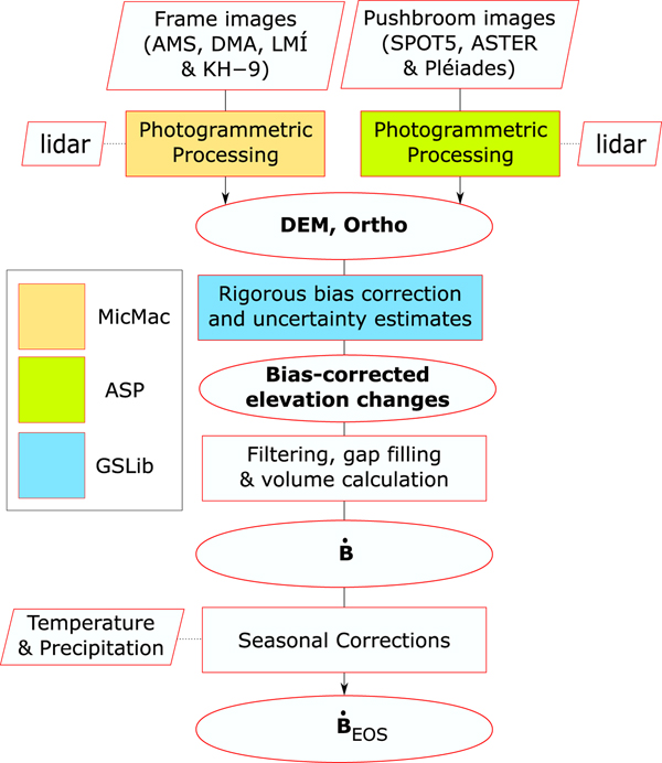


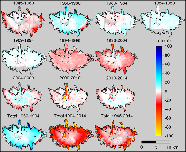


 Open access