


Introduction
The Antarctic Peninsula (AP), particularly the northern and north-western AP, is one of the polar regions that has experienced a pronounced and statistically significant warming since 1950 (e.g. Turner et al. Reference Turner, Phillips, Hosking, Marshall and Orr2013, Reference Turner, Marshall, Clem, Colwell, Phillips and Lu2019, Clem et al. Reference Clem, Renwick, McGregor and Fogt2016, Tetzner et al. Reference Tetzner, Thomas and Allen2019, Carrasco et al. Reference Carrasco, Bozkurt and Cordero2021, Flexas et al. Reference Flexas, Thompson, Schodlok, Zhang and Speer2022, Gorodetskaya et al. Reference Gorodetskaya, Durán-Alarcón, González-Herrero, Clem, Zou and Rowe2023, IPCC Reference Lee and Romero2023), and it is often considered the site of the most intense climate change in Antarctica. Meteorological observations over Antarctica began mostly in the International Geophysical Year (1957–1958), and although records are not as abundant as in other world regions, they are becoming sufficient to quantify climate variability and change and to provide important information on climate controls in the region (King et al. Reference King, Turner, Marshall, Connolley and Lachlan-Cope2003), serving to improve our understanding of regional climate processes. These data have suggested that both AP and West Antarctica have experienced dramatic climate changes (Monaghan et al. Reference Monaghan, Bromwich, Chapman and Comiso2008, Fogt et al. Reference Fogt, Bromwich and Hines2011, Clem et al. Reference Clem, Renwick, McGregor and Fogt2016), with AP being the region where the largest degree of climate variability on the continent has been observed (King Reference King1994, King et al. Reference King, Turner, Marshall, Connolley and Lachlan-Cope2003), demonstrating the greatest warming trends over the entire continent (Ferron et al. Reference Ferron, Simões, Aquino and Setzer2004, Clem et al. Reference Clem, Renwick, McGregor and Fogt2016, Tetzner et al. Reference Tetzner, Thomas and Allen2019, Turner et al. Reference Turner, Marshall, Clem, Colwell, Phillips and Lu2019). For instance, Esperanza Station has warmed by 0.29°C ± 0.16°C per decade during 1957–2016 (Gorodetskaya et al. Reference Gorodetskaya, Durán-Alarcón, González-Herrero, Clem, Zou and Rowe2023).
The IPCC Sixth Assessment Report (AR6) states clearly that one of the impacts of climate change and increasing global temperatures constitute changes in extreme events, such as heatwaves (Collins et al. Reference Collins, Sutherland, Bouwer, Cheong, Frölicher and Jacot Des Combes2019). Heatwaves are usually associated with persistent atmospheric ‘blocking’ systems or quasi-stationary circulation anomalies (Chan et al. Reference Chan, Catto and Collins2022). It is already known that large-scale atmospheric circulation patterns and atmospheric dynamics themselves are important drivers of local and regional extremes, and that they modulate the magnitude, frequency and duration of such extremes (Seneviratne et al. Reference Seneviratne, Zhang, Adnan, Badi, Dereczynski and Di Luca2021). Atmospheric blocks can have varying configurations, amplitudes and durations and do not always result in heatwaves, but they play a crucial role in generating warm events (WEs) when located in such a way that they drive anomalous and sustained warm advection (Chan et al. Reference Chan, Catto and Collins2022). In the Southern Ocean, this type of blocking can interact with the Amundsen Sea Low, facilitating the transport of warm and moist air from the mid-latitudes towards Antarctica, often in the form of atmospheric rivers (Carrasco et al. Reference Carrasco, Bozkurt and Cordero2021, Bozkurt et al. Reference Bozkurt, Marín and Barrett2022, Gorodetskaya et al. Reference Gorodetskaya, Durán-Alarcón, González-Herrero, Clem, Zou and Rowe2023). Extreme warm episodes in Antarctica are particularly important given that Antarctica’s ice might melt if temperatures increase to the melting point of the ice (Gonzalez-Herrero et al. Reference González-Herrero, Navarro, Pertierra, Oliva, Dadic, Peck and Lehning2024). This could have significant and immediate impacts on the cryosphere by inducing positive feedbacks that accelerate such warming trends (Seneviratne et al. Reference Seneviratne, Zhang, Adnan, Badi, Dereczynski and Di Luca2021, Gorodetskaya et al. Reference Gorodetskaya, Durán-Alarcón, González-Herrero, Clem, Zou and Rowe2023).
In recent years, Antarctica has experienced several remarkable extreme events. On 24 March 2015, a record high of 17.5°C was recorded at the northern end of AP, at the Argentine Esperanza Station, 1 day after 17.4°C was measured at the Argentine Marambio Station, ~100 km south-east of Esperanza. The 17.5°C event took place during a period of warm air advection with a north-westerly circulation anomaly, and at that time it represented the highest temperature recorded for the Antarctic continent (Skansi et al. Reference Skansi, King, Lazzara, Cerveny, Stella and Solomon2017). During the summer of 2019/2020, a sequence of anomalously high temperatures affected much of Antarctica, leading to ice melting and the exposure of new ice-free areas. In early February 2020, a new record high temperature was observed over AP and its surrounding islands, which experienced one of its longest recorded heatwaves and with a wide spatial extent, culminating in an 18.3°C record at Esperanza Station on 6 February 2020, which represented an anomaly of 8°C, almost 1°C warmer than the previous record of 17.5°C (González-Herrero et al. Reference González-Herrero, Barriopedro, Trigo, López-Bustins and Oliva2022). This 6 day heatwave was associated with anomalous circulation patterns, driven by a stationary high-pressure system in the Drake Passage, and it was declared by the World Meteorological Organization as the new maximum temperature record for the continent. The latest and most recent record was the extreme event on 18 March 2022, when the temperature at Dome C on the Antarctic Plateau (East Antarctica) reached a temperature of −10.1°C, more than 40°C above the seasonal norm. This unprecedented heatwave between 15 and 19 March 2022 became one of the largest short-term temperature jumps on record, with a scale and intensity never observed before (Blanchard-Wrigglesworth et al. Reference Blanchard-Wrigglesworth, Cox, Espinosa and Donohoe2023, Wille et al. Reference Wille, Alexander, Amory, Baiman, Barthélemy and Bergstrom2024).
In this context, the present work seeks to analyse the daily extreme warm temperature events around Maxwell Bay, King George Island (KGI), and the associated atmospheric circulation patterns for the period between 1998 and 2016. This involves the construction and use of a temperature database from the Artigas Antarctic Scientific Base (BCAA, Uruguay), which to date has not been used and thus has not undergone quality control. The study of extreme events requires reliable databases, at least on a daily scale. In that regard, to facilitate the study of extremes over Antarctica, the Scientific Committee on Antarctic Research (SCAR) has promoted since the late 1990s the generation of databases from all Antarctic weather stations, based on 6 h synoptic observations (Turner et al. Reference Turner, Marshall, Clem, Colwell, Phillips and Lu2019). The project is known as Reference Antarctic Data for Environmental Research (READER; https://www.scar.org/resources/ref-data-environmental-research), but to date BCAA does not form a part of this project because it has never been quality controlled. Thus, this study, in addition to the previously mentioned objectives, aims to generate a quality daily database to be uploaded to SCAR-READER.
The manuscript is structured as follows: the section ‘Data and methodology’ describes the study area, the construction of the daily temperature database and the analytical approach applied in this work. The section ‘Results’ presents a climatological characterization of the temperature series and its variability at annual and interannual scales, followed by an analysis of warm and extreme warm events (EWEs) detected at the three Antarctic stations and the associated atmospheric circulation anomalies. The section ‘Discussion’ interprets these findings in the context of climate variability and large-scale circulation patterns. Finally, the section ‘Summary and conclusions’ provides the main outcomes and perspectives for future research.
Data and methodology
Study region
KGI is located 120 km north-north-west of AP, and it is the largest island of the South Shetland Archipelago. Located between 61°54´/62°16´S and between 57°35´/59°02´W, with an estimated area of 1310 km2 (95 km long and 25 km wide), KGI has three large bays: Maxwell Bay (also known as Fildes Bay), at 19 km long and located to the south-west of the island; Admiralty Bay, which is more irregular in shape and is located on the south coast; and King George Bay, at 11 km long on the south-south-east coast. Approximately 90% of the island is permanently covered by an ice cap that forms five large domes (Rückamp et al. Reference Rückamp, Braun, Suckro and Blindow2011). Most of the ice cap perimeter ends in the Southern Ocean in the form of large outlet glaciers to the sea both to the south and north of the island (Macheret & Moskalevsky Reference Macheret and Moskalevsky1999, Moll & Braun Reference Moll and Braun2006, Osmanoglu et al. Reference Osmanoglu, Braun, Hock and Navarro2013). Only a few glaciers, mainly the smaller ones, end up on land (Moll & Braun Reference Moll and Braun2006). One of them is Collins Glacier, also known as Bellingshausen Dome (Braun et al. Reference Braun, Esefeld and Peter2017), a small ice dome at 15 km2 in area, with an average thickness of 65 m and 270 m maximum elevation (located in the north-eastern region of the Dome; Rückamp & Blindow Reference Rückamp and Blindow2012, Simões et al. Reference Simões, Da Rosa, Czapela, Vieira and Simões2015, Petsch et al. Reference Petsch, Da Rosa, Vieira, Braun, Mattos Costa and Simões2020). Fildes Peninsula, at ~29 km2, is the largest ice-free area of the entire island (Petsch et al. Reference Petsch, Da Rosa, Vieira, Braun, Mattos Costa and Simões2020), with Collins Glacier located to the north of the peninsula. These characteristics make this glacier one of the most studied on the island. The observations analysed in the present study come from scientific bases located around Maxwell Bay, with two of them on Fildes Peninsula (Fig. 1).
Geographical locations of the study area and research stations. (Left) Antarctic Peninsula and South Shetland Islands. (Middle) King George Island within the South Shetland Islands. (Right) Locations of the stations considered in this study: Artigas Antarctic Scientific Base (BCAA; blue) and C.M.A. Eduardo Frei Montalva (FREI; pink) on Fildes Peninsula, and King Sejong (KS; yellow) on the opposite side of Maxwell Bay.

Data
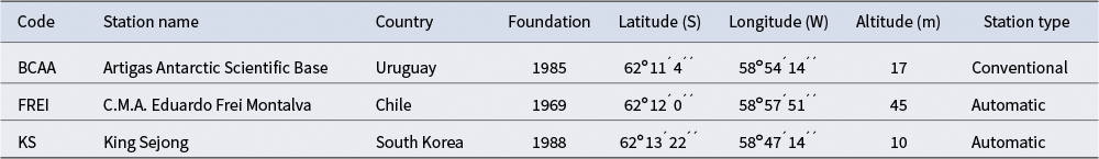
In this study we used synoptic observations of surface temperature data from three meteorological stations across Maxwell Bay in KGI: Artigas Antarctic Scientific Base (BCAA, Uruguay), C.M.A. Eduardo Frei Montalva (FREI, Chile) and King Sejong (KS, South Korea; Table I). The datasets span the period 1998–2016 for the four main synoptic hours: 00, 06, 12 and 18 Coordinated Universal Time (UTC).
Antarctic stations used for this study. Station identification code (generated for this work as an abbreviation of the station name), complete name, country, year of foundation, geographical location, altitude and station type are detailed.

The meteorological information from the Korean base was obtained using an automatic weather station and was provided by the Korea Polar Research Institute (KOPRI) with exhaustive quality control. The Chilean weather station data also come from an automatic station; these data are not quality controlled but are nevertheless considered good quality by the Chilean Meteorological Service (Dirección Meteorológica de Chile) and are widely used. The data were obtained through the Climate Services Portal of the National Weather Service of Chile.
The data from BCAA were provided by the National Weather Service, Uruguayan Institute of Meteorology (INUMET). They were obtained from Meteorological Station No. 89054 according to the World Meteorological Organization (WMO) list, located at 62°11´04´´S, 58°51´07´´W, at an altitude of 17 m above sea level. The meteorological station is classified as conventional, although at present there is an automatic station here that operates without personnel. KS base is located at 62°13´22´´S, 58°47´14´´W (WMO Code No. 89251) at 10 m above sea level and is visible from BCAA, but both stations are separated by Maxwell Bay and Collins Glacier, at a linear distance of ~8 km. Finally, the Chilean weather station is located at 62°19´S, 58°98´W (WMO Code No. 89056) at 45 m above sea level and at a linear distance to BCAA of ~4 km.
For the atmospheric circulation analysis, reanalysis data were used, as such observations can be used for the same purposes as in situ data (Parker Reference Parker2016, Tetzner et al. Reference Tetzner, Thomas and Allen2019). This dataset becomes of great importance particularly in Antarctica, as in situ data are relatively poor due to the sparse network of observing stations. In the present work, monthly data from the National Centers for Environmental Prediction (NCEP)/National Center for Atmospheric Research (NCAR) Reanalysis project (Kalnay et al. Reference Kalnay, Kanamitsu, Kistler, Collins, Deaven and Gandin1996) were used for the variables of temperature, wind and pressure at surface level and geopotential height at the 500 hPa level (z500). The data are spatially distributed on a grid of 0.25° latitude by 0.25° longitude, and they correspond to the region between latitudes 30°S and 90°S and longitudes −180°W and 180°E. The data were downloaded from the website of the Physical Sciences Laboratory (https://psl.noaa.gov/data/gridded/data.ncep.reanalysis.html) of the National Oceanic and Atmospheric Administration (NOAA), a US service.
We also used indices that represent two of the most important modes of variability in the Antarctic region. For the El Niño Southern Oscillation (ENSO) we used the Oceanic Niño Index (ONI) from NOAA (https://origin.cpc.ncep.noaa.gov/products/analysis_monitoring/ensostuff/ONI_v5.php) to classify El Niño (warm) and La Niña (cold) events based on the mean sea-surface temperature (SST) anomaly of the Niño 3.4 region for 3 consecutive months. The Southern Annular Mode (SAM) Index developed by Marshall (Reference Marshall2003) was used for the estimation of SAM phases during EWEs. It is based on the normalized monthly sea-level zonal pressure difference between six stations located at latitude 40°S and six stations at latitude 65°S at monthly, seasonal and annual time scales.
BCAA daily database construction
BCAA was established in December 1984 on Fildes Peninsula, KGI, marking the beginning of Uruguay’s permanent presence in Antarctica. Since then, the station has been in continuous operation, with scientific activities carried out mainly during the summer. Meteorological observations began in 1985, but these data had never previously been processed or analysed. In addition to the conventional station, an automatic weather station has been operating at BCAA since the 2000s, but, due to numerous discontinuities, its records were discarded. In this study, we conducted the first comprehensive quality control of the daily temperature series from the conventional station at BCAA. The quality control procedure consisted of five stages:
-
1) Time homogenization: BCAA records were provided in local time (UTC - 3) at 03h00, 09h00, 15h00 and 21h00, and were converted to UTC (00, 06, 12 and 18 UTC), being the standard used internationally. Records outside these reference hours were excluded (359 in total). Data from FREI and KS were already in UTC.
-
2) Sequencing check: The datasets were manually reviewed to ensure four records per day (00, 06, 12 and 18 UTC) were obtained. Missing observations (date and time) were inserted as ‘NA’ entries. This resulted in 1350 missing entries at BCAA, 89 at FREI and 0 at KS. We also eliminated date from 29 February of leap years, so that every year had 365 days. Finally, all three datasets comprised 27 660 dates.
-
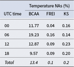
3) Missing data analysis: BCAA presented the highest proportion of missing values (13.4%), distributed heterogeneously throughout the series. In contrast, FREI and KS were substantially more complete (< 0.5% missing values). Table II presents the hourly and total missing data from the three stations.
-
4) Range check (outliers): Two complementary range tests were applied to identify unrealistic temperature values. First, fixed thresholds (−40°C to 20°C), defined from historical extremes in the South Shetland Islands (Nowosielski 1980, Rusticucci & Barrucand 2001, Bañón et al. 2013), ensured that no observations exceeded the physically impossible or never-before-observed values in the historical record (Veiga et al. Reference Veiga, Herrera, Skansi and Podestá2015). No such values were found. Second, variable seasonal thresholds were calculated. Following the methodology applied in Rusticucci & Renom (Reference Rusticucci and Renom2007) and WMO (2018), we calculated the monthly climatology for the whole series and determined a seasonal range placing as upper and lower limits four times the standard deviation (SD; mean ± 4 SD), allowing the detection of unusual values relative to the expected climatological variability. This test flagged 83 records at BCAA (0.34% of the series). Each case was verified against INUMET’s original handwritten logbooks and also compared with nearby stations (FREI and KS). Most flagged values were either consistent with the neighbouring series or identified as typographical errors and were accordingly corrected or retained, without increasing the number of missing values.
-
5) Temporal consistency check: Differences between consecutive observations were tested to ensure realistic changes between consecutive records (Ye et al. Reference Ye, Yang, Xiong, Yang and Chen2017, WMO 2018). A new time series was constructed using the absolute differences between each record and its immediate predecessor (∆X = |Xi - X i - 1|). A dynamic threshold was then defined as (series mean ± 4 SD) (Renom Reference Renom Molina2009), against which all differences were evaluated. Values exceeding this limit were flagged as potential errors and subsequently verified against original records and the neighbouring stations (FREI and KS). At BCAA, 205 temperature cases exceeded thresholds: 178 of them were accepted, as they were also recorded in the FREI and/or KS databases. The remaining 27 were typographical errors and were afterwards corrected by INUMET, so no value was lost.
Percentage of missing data (NAs) per hour for temperature for stations Artigas Antarctic Scientific Base (BCAA), C.M.A. Eduardo Frei Montalva (FREI) and King Sejong (KS) and total percentage of NAs in relation to total data.

UTC = Coordinated Universal Time.
After completing the range and temporal consistency checks, a final spatial consistency analysis was performed to assess the coherence between BCAA and the nearby stations FREI and KS, as well as to explore the possibility of reconstructing missing records. Given the non-normal distribution of the variable (see the ‘Climate at BCAA’ subsection that follows), pairwise correlations were calculated using Spearman’s rank correlation coefficient (ρ). In both cases, correlations were positive, statistically significant (α = 0.05) and very strong (ρ = 0.98, P < 0.001), indicating that the three stations exhibit almost identical temporal variability.
Based on this strong spatial coherence, the missing values at BCAA were filled using the mean of the simultaneous (day and time) FREI and KS observations, computed with the rowMeans function of the base package in R (RStudio Team 2021). This averaging approach was preferred over regression-based or moving-average interpolations for several reasons: 1) the records are available every 6 h in a highly variable polar environment, 2) many of the data gaps consist of several consecutive records and 3) regression-based or moving-average imputation under such conditions could introduce artificial trends or distort the intrinsic variability of the regional climate system, or the ‘variability structure’. As the objective was to obtain a spatially consistent and homogeneous dataset suitable for subsequent climatological analysis, this method provided the most conservative and transparent solution.
To evaluate the potential uncertainty introduced by this procedure, the difference between observed BCAA values and the mean of FREI and KS values was calculated for periods with complete records. The mean bias was 0.1°C and the mean absolute difference was 0.5°C, indicating a very close agreement between the observed and reconstructed values. These small differences confirm that the averaging method preserves the representativeness of the BCAA series while minimizing the uncertainty associated with missing data. The slight geographical differences among the stations may explain part of the residual variance but do not significantly affect the overall coherence of the datasets.
Seasonal definition based on solar forcing
Given the pronounced annual cycle of solar radiation at high southern latitudes, seasonal analysis in this study were conducted using a photoperiod-based classification rather than temperature-defined months. Accordingly, the year was divided into two 6 month periods that reflect the local solar forcing: the ‘warm season’ (September–February), characterized by 12 or more hours of daylight, and the ‘cold season’ (March–August), with 12 or fewer hours of daylight. This approach captures the role of solar radiation and daylight duration on the surface energy balance and, consequently, the seasonal temperature response to these radiative changes in the polar regions.
Detection of warm and extreme warm events
WEs and EWEs were identified using a percentile-based approach consistent with international standards for climate extremes (WMO 2009, 2023). A WE was defined as a period of at least 3 consecutive days with daily mean temperatures above the 90th percentile, while an EWE exceeded the 99th percentile. Percentile thresholds were calculated from the 1998–2016 daily mean temperature series using a 5 day moving window centred on each calendar day, following the recommendations of the Expert Team on Climate Change Detection and Indices (ETCCDI) to account for the local seasonal cycle and to minimize running-window bias.
These percentiles were used solely as climatological thresholds to identify anomalously warm days. The actual number of detected events depends on the persistence criterion (≥ 3 consecutive days), which is governed by synoptic-scale circulation variability. Consequently, frequency is not evenly distributed throughout the year, and the proportion of days belonging to WEs or EWEs can differ from the nominal 10% or 1% implied by the percentile threshold.
Once the events were detected, they were manually reviewed to verify the absence of duplicated events and to ensure temporal congruence between the three stations (BCAA, FREI and KS). All events detected at FREI and/or KS that occurred within ± 2 days of the start date of an event detected at BCAA were considered to represent the same regional event. When the event spanned 2 months, it was assigned to the month of onset, except when the event began on the last or penultimate day of a month and extended for more days into the following month; in such a case, it was assigned to the latter.
Results
Climate at BCAA
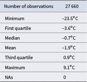
After constructing the daily temperature database for BCAA, a climatological analysis of the series was performed. The histograms of daily mean temperatures show a non-normal distribution (Shapiro-Wilk test, P < 2.2e−16), skewed to the right (Fig. 2). All three stations exhibit similar distributions, with higher frequencies in the range between −2°C and 2°C. At BCAA and KS, most values fall between 0°C to 2°C, whereas at FREI they concentrate between the −2°C to 0°C range. The BCAA series presents a skewness of −1.34 and kurtosis of 4.95, indicating a leptokurtic distribution with heavier tails relative to a normal one, as shown in Fig. 2a. The maximum temperature recorded was 9.1°C on 25 January 2004, and the minimum was −23.5°C on 15 July 2007, both also detected at the nearby stations. Table III summarizes the statistical properties of the daily mean temperature distribution at BCAA.
Histograms of daily mean air temperatures for the three stations: a. Artigas Antarctic Scientific Base (BCAA; orange), b. C.M.A. Eduardo Frei Montalva (FREI; green) and c. King Sejong (KS; violet).

Statistical summary of daily mean air temperatures for Artigas Antarctic Scientific Base (BCAA) after the process of completing the missing data (NAs).

At the hourly scale, temperature shows strong variability throughout the year, particularly from June to September, with the widest spread occurring in July (Fig. 3). The smallest interquartile range occurs at 18 UTC and the largest at 6 UTC. July displays the highest interquartile range at 0 UTC (7.1°C). January and December have the lowest variability. Thermal amplitude is greatest at 0 UTC (32.6°C) and smallest at 6 UTC (28.5°C). No significant differences were found among the four synoptic hours, indicating that the daily means adequately represent the temperature behaviour.
Annual cycles of the hourly temperature (Temp) distribution by schedule (0, 6, 12 and 18 Coordinated Universal Time (UTC)) at Artigas Antarctic Scientific Base (BCAA). The red dotted lines represent 0°C.

The annual cycle of air temperature is characterized by monthly mean values between −5.6°C and 1.7°C, with an annual average of −1.9°C. Positive values are observed from December to March and negative values from April to November, with July being the coldest month and January the warmest (Fig. 3). The steep drop from May to June stands out. Daily thermal amplitude is minimal in the coldest months (April–July), increasing thereafter as daylight duration lengthens. By August, daily amplitude rises noticeably due to ~3 additional daylight hours. January and December show the largest daily amplitudes (1.6°C and 1.3°C, respectively, between 6 and 18 UTC).
Annual variability and trend
Annual anomalies were obtained by subtracting the climatological mean from the annual mean of each year. Of the 19 years analysed, 10 of them presented positive anomalies and 9 negative ones, with 2014 being close to the mean. The first half of the record is dominated by positive anomalies, with 1999 and 2008 being the warmest years (0.8°C and 0.9°C above average, respectively). Conversely, the second half of the series is dominated by negative anomalies, mostly below −0.5°C (Fig. 4). The linear trend in monthly mean temperature is negative (−0.1°C per year) but not statistically significant at the 95% confidence level (P = 0.11).
Annual temperature (Temp) anomalies. Red bars represent positive anomalies and blue bars represent negative anomalies.

Interannual variability
To assess seasonal variability, the year was divided into the four conventional meteorological seasons: summer (DJF), autumn (MAM), winter (JJA) and spring (SON). Summers are named by the year corresponding to the month of December.
Summer is the warmest season and winter the coldest, with climatological means of 1.3°C and −5.3°C, respectively. Summer exhibits the least interannual variability (−1.1°C to 1.2°C), whereas winter shows the greatest (−2.7°C to 1.8°C). A statistically significant cooling trend was detected in summer (−0.1°C per year, P = 0.0026). Autumn (−1.0°C) and spring (−2.4°C) show similar mean values, although spring occasionally reached autumn-like temperatures during 2008, 2010 and 2016, when large positive anomalies occurred. The warmest years were 1999 and 2008, when all four seasons presented positive anomalies, whereas 2007 was the coldest, with particularly low autumn and winter temperatures. Seasonal anomalies usually alternate in sign throughout the year (Figs 4 & 5).
Temperature (Temp) anomalies for the four seasons: summer (DJF, upper left), autumn (MAM, upper right), winter (JJA, lower left) and spring (SON, lower right). Red bars represent positive anomalies and blue bars represent negative anomalies.

When grouped into extended seasons, the cold season (March–August) presents larger anomalies (−2.4°C to 1.4°C) than the warmer season (September–February; −1.0°C to 1.1°C). Some years show opposite anomalies between seasons (e.g. 1998, 2000, 2003, 2005, 2011, 2013 and 2014). Regarding the warm season, particularly warm years were 2008 (> 1°C above the climatic average), 2001 (0.9°C) and 2010 (0.8°C). In addition, the warm seasons of 2012, 2015 and 2009 showed negative anomalies of −1.0°C, −0.9°C and −0.8°C, respectively. In the cold season, marked negative anomalies were observed in 2007 (> 2°C below the climatological mean), 2011 (−1.7°C) and 2009 (−1.3°C). Finally, the two largest anomalies of the entire series (2007: negative; 2008: positive) were reflected in both extended seasons. The 2007 negative anomaly was mainly driven by exceptionally cold conditions during the cold season, whereas in 2008 both seasons were warm, but the warm season showed a much stronger positive anomaly (Fig. 6).
Temperature (Temp) anomalies for the cold (upper) and warm (lower) seasons. The red bars represent positive anomalies and the blue bars represent negative anomalies.

Warm and extreme warm events
WEs were detected throughout the year, with a higher number of occurrences during the cold season, particularly in June (Fig. 7). Over half of the events recorded at BCAA were simultaneous at all three stations, while 13 events (out of 101) were unique to BCAA. Nine events were shared exclusively by FREI and KS, and each station independently registered 15 events.
Monthly distribution of warm events for the three stations: Artigas Antarctic Scientific Base (BCAA), C.M.A. Eduardo Frei Montalva (FREI) and King Sejong (KS).

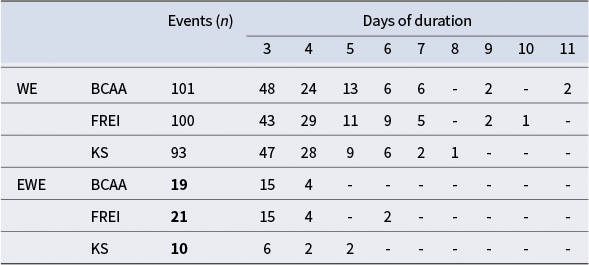
In terms of duration, most WEs lasted between 3 and 4 days, with 3 day events being the most common (Table IV). KS did not record events longer than 8 days, while only BCAA experienced two events lasting 11 days (17 September 2003 and 23 November 2008). Cold-season WEs tended to persist longer than warm-season ones.
Frequencies of events discriminated by intensity (warm events (WEs) and extreme warm events (EWEs)) and by station (Artigas Antarctic Scientific Base (BCAA), C.M.A. Eduardo Frei Montalva (FREI) and King Sejong (KS)), detailing the total number of events and the number of events according to days of duration. Events above the 99th percentile are shown in bold.

The largest temperature anomalies (> 5°C above the climatological mean) also occurred predominantly during the coldest months, mainly between June and September. June showed the highest number of such events (12 at BCAA, 11 at FREI and KS), and this was also the month with the greatest spatial coherence across the stations (11 concurrent events). Other active months included September, November and March, each with at least 10 detected WEs at BCAA (Fig. 7).
Regarding intensity, the temperature anomalies ranged from 1.1°C to 6.5°C. March exhibited the largest number of extreme anomalies, with eight outliers between 4.8°C and 6.1°C, followed by November with six outliers (2.5–4.8°C). Several winter events showed mean anomalies exceeding those of summer events.
At BCAA, 54 WEs occurred during the cold season, consistent with the monthly distribution. The years 2009, 2012, 2014 and 2015 lacked WEs during the warm season, whereas cold-season events occurred every year except 2015. The warm season exhibited alternating years of high and low event occurrence, whereas the cold season showed more frequent and persistence activity during the first half of the record (1998–2006).
Only two EWEs were shared among the three stations (18 June 1998 and 7 August 2003), both in the cold season. Five EWEs at BCAA were shared only with FREI, six only with KS and six were unique to BCAA. FREI recorded 14 independent events and KS recorded two such events. All EWEs at BCAA lasted between 3 and 4 days (Table IV). KS recorded two 5 day events (9 June 1999 and 27 August 2012), and FREI recorded two 6 day events (15 May 2000 and 28 August 2003).
The years 1998, 2006 and 2008 exhibited the highest number of EWEs (Fig. 8), with up to four such events recorded at BCAA in 2008 and at FREI in 2006. No such events occurred in 2002, 2009, 2010, 2013, 2014 and 2015.
Annual distribution of extreme warm events for the three stations: Artigas Antarctic Scientific Base (BCAA), C.M.A. Eduardo Frei Montalva (FREI) and King Sejong (KS).

EWEs occurred throughout the year, except during the warmer months: February showed none, and January showed only one at KS. August had the highest number of EWEs (three at BCAA and KS, two at FREI). At BCAA, the months with the highest number of EWEs were May, July, August and October (three each). Consistent with WEs, EWE occurrences were greater in the cold season (13) than in the warm season (6). The only year with warm-season EWEs at all three stations was 2006 (one event each). One of these (19 October 2006) was shared by BCAA and KS, lasted 3 days and reached a positive anomaly of 3.5°C. Additional warm-season EWEs occurred at BCAA in 2008 (three events) and 2016 (two events): one in 2008 (15 September 2008) was shared with KS and reached an anomaly of 4.5°C, and one in 2016 (4 September 2016) was shared with FREI and reached an anomaly of 5.8°C.
During the cold season, EWEs were recorded simultaneously at the three stations in 1998, 2003 and 2012, with BCAA showing two events per year in 1998 and 2012. The events of 18 June 1998 and 7 August 2003 lasted 4 days; the first one reached a mean temperature of 1.1°C (6.4°C above the daily climatological mean of −5.3°C). As with WEs, cold-season EWEs tended to last longer than warm-season ones, with durations of up to 6 days at FREI, whereas at BCAA both warm- and cold-season EWEs had a maximum persistence of 4 days (Fig. 9).
Days of duration of warm events (WEs; upper images) and extreme warm events (EWE; lower images) for the warm (left) and cold (right) season for the three stations: Artigas Antarctic Scientific Base (BCAA), C.M.A. Eduardo Frei Montalva (FREI) and King Sejong (KS).

Atmospheric circulation anomalies associated with extreme warm events
A detailed analysis of the spatial pattern of EWEs was conducted by constructing composites of the reanalysis data using the 1991–2020 climatology, including only months with two or more events. January, February and April were excluded due to insufficient cases. The resulting maps revealed a consistent spatial pattern associated with EWE occurrence (Fig. 10). In all cases, surface temperature anomalies extended beyond KGI, with the anomaly centre generally located to the east of AP. Only a few months (mainly mid- and late winter and occasionally early summer) showed deviations from this pattern, with the anomaly centre displaced towards or west of AP or over southern South America.
Monthly composites of anomalies of the following variables: a. surface air temperature (Temp.), b. surface wind vector, c. sea-level pressure (SLP) and d. geopotential (Geop.) at 500 hPa. To simplify the graphical representation, we show only June and October composites, as these were the months with the highest number of events (five each). The data have a daily resolution, and the anomalies were constructed based on the climatology of the period 1991–2020 obtained from the National Oceanic and Atmospheric Administration (NOAA) Physical Sciences Laboratory in Boulder, CO, USA (https://psl.noaa.gov/data/composites/day/).

These positive temperature anomalies in the AP region were accompanied by a pressure dipole, with low pressure to the west (blue to violet in Fig. 10) and high pressure to the east of the peninsula (yellow to red in Fig. 10), producing northerly warm advection, with intensities up to 10 or 12 m/s above average.
Most EWEs occurred during La Niña years according to the ONI index, as well as during positive SAM phases according to the SAM index (Table V). Correlation analyses between the mean monthly temperature anomalies and the ONI/SAM indices for June and October were performed. These months were selected as they had the highest number of extreme events (five each). The results showed a negative and statistically significant relationship with ONI and a positive but non-significant relationship with SAM. The correlations were slightly higher for October than for June, and, in turn, they were higher for BCAA than for the other stations.
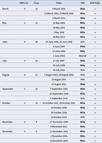
Extreme warm events (EWEs) used for composites. The number of events per month is detailed, as well as the start date of each event and the total number of monthly days used for each composite. The Oceanic Niño Index (ONI) column classifies the year according to the temperature anomaly of the quarter consisting of November, December and January. Negative anomalies (Niña events) are highlighted in bold, positive anomalies (Niño events) are highlighted in italics and neutral events in given in standard text.

SAM = Southern Annular Mode.
Discussion
The results show that temperatures at BCAA reveal a cooling tendency during the second half of the studied period, consistent with previous studies reporting a temporary reversal of the late twentieth-century warming trend over AP (Turner et al. Reference Turner, Lu, White, King, Phillips and Hosking2016, Oliva et al. Reference Oliva, Navarro, Hrbáček, Hernández, Nývlt and Pereira2017, Gonzalez & Fortuny Reference Gonzalez and Fortuny2018). Cooling rates between −0.47 ± 0.25°C decade−1 (1999–2014; Turner et al. Reference Turner, Lu, White, King, Phillips and Hosking2016) to −0.67°C decade−1 (2000–2016) have been observed, with values up to −1.63°C (2008–2015) found in some records (Gonzalez & Fortuny Reference Gonzalez and Fortuny2018). At KS, located in the South Shetland Islands and one of the stations used in the present study, the decade 2006–2015 was 0.6°C colder than the preceding one (1996–2005; Oliva et al. Reference Oliva, Navarro, Hrbáček, Hernández, Nývlt and Pereira2017), supporting the regional coherence of this cooling signal.
This cooling is primarily attributed to natural internal variability and large-scale atmospheric and oceanic drivers. Turner et al. (Reference Turner, Lu, White, King, Phillips and Hosking2016) linked it to increased cyclonic activity over the west of AP, associated with a strengthening of the Polar Front Jet under the negative phase of the Interdecadal Pacific Oscillation and more frequent La Niña conditions. These mechanisms intensified meridional temperature gradients and favoured cold easterly advection from the Weddell Sea. Oliva et al. (Reference Oliva, Navarro, Hrbáček, Hernández, Nývlt and Pereira2017) further noted that strong El Niño episodes (such as 1982–1983 and 1998) were typically followed by several years of below-average temperatures, suggesting that these events may act as turning points modulating decadal temperature variability. According to Gonzalez & Fortuny (Reference Gonzalez and Fortuny2018), the recent cooling episode is statistically consistent with the internal decadal variability of the AP climate system, and its short duration (~20 years) makes it unlikely to represent a sustained reversal.
The interannual anomalies identified in this study, particularly the cold 2007 and warm 2008, can also be interpreted in the context of ENSO evolution during that period. According to NOAA’s monitoring reports, 2007 began under weak El Niño conditions but transitioned into strong La Niña conditions by mid-year, peaking in early 2008. Such transitions are relevant to AP, where the ENSO modulates surface temperatures via large-scale circulation and the Amundsen Sea Low (Clem & Fogt 2013). Our results are consistent with the findings of Clem et al. (Reference Clem, Renwick, McGregor and Fogt2016), who showed that ENSO-SAM interactions play a key role in modulating interannual temperature variability across AP and the South Shetland Islands, with the combined phase determining whether warm maritime advection is favoured or suppressed in a given season.
The analysis of atmospheric surface circulation during EWEs in our datasets consistently exhibits a surface-pressure dipole: a low centred to the west of AP and a high to the east, with the consequent generation of anomalous northerly flow and warm advection over the South Shetland Islands. This spatial configuration is consistent with blocking-like situations near the Drake Passage that sustain advection over several days. Event persistence showed no clear annual pattern, although the longest WEs occurred in spring and late winter (up to 11 days in September/November; up to 9 days in May/August). Importantly, our correlation analysis between monthly temperature anomalies and ONI (for MJJ and SON) shows a significant negative relationship (warmer anomalies associated with more negative ONI values), whereas the correlation with SAM was positive but not significant. However, although the latter is not statistically significant (probably due to the limited sample size), it is important to highlight that most EWEs occurred during the positive phase of SAM, and previous studies (e.g. Fogt & Marshall Reference Fogt and Marshall2020) have reported a positive and significant relationship between the monthly mean surface temperature over the western AP and the SAM positive phase.
Finally, the strong spatial coherence observed among BCAA, FREI and KS during many WEs indicates that WEs are often regional-scale phenomena linked to synoptic circulation patterns rather than isolated local episodes. The events detected at a single station probably reflect local surfaces influences (e.g. proximity to glaciers) or sub-synoptic variability. This highlights the importance of maintaining multiple nearby stations to better resolve spatial temperature gradients and to improve our understanding of the underlying processes.
Summary and conclusions
A reliable 6 h temperature database was developed for BCAA through an exhaustive quality-control process. The resulting dataset, consistent with nearby stations FREI and KS, allowed the construction of a robust temperature climatology and a first regional assessment of WEs and EWEs on KGI.
The analysis showed marked seasonal and interannual variability, with the cold season displaying the largest temperature anomalies and variability. WEs were detected almost every year except for 2015, with the highest occurrence in June and the longest events lasting up to 11 days. EWEs were less frequent but often were regionally coherent, typically being associated with a surface-pressure dipole that generated anomalous northerly warm advection over the South Shetland Islands.
This study constitutes a first approach to the characterization of WEs and EWEs in the region and provides a baseline for future analyses of extreme temperature behaviour. The new BCAA dataset will be proposed for inclusion in the READER project of the SCAR, contributing to the Antarctic climate data network and enhancing the availability of national observations to the international scientific community.
Future work will focus on a more detailed examination of the duration, intensity and atmospheric circulation patterns associated with these events, as well as their potential impacts on local environments. The same methodology could also be applied to identify extreme cold events, defined as periods when the daily mean temperature falls below the 10th percentile for 3 or more consecutive days, and to explore in greater depth the role of the large-scale climate modes such as the ENSO and SAM in modulating both warm and cold events.
Acknowledgements
We thank the Uruguayan Institute of Meteorology (INUMET in Spanish) for providing the data used in this research, and the Uruguayan Antarctic Institute (IAU in Spanish) for facilitating communication with the other Antarctic stations and supporting the data acquisition process. Finally, we acknowledge the National Programme for the Development of Basics Sciences (PEDECIBA in Spanish), subarea of geosciences, for its role in supporting both this work and the professional development of the first author.
Financial support
We gratefully acknowledge the National Agency for Research and Innovation (ANII in Spanish) and the Postgraduate Academic Commission of the University of the Republic (CAP in Spanish) for the financial support that made this work possible.
Competing interests
The authors declare no competing interests.
Author contributions
FB carried out the analyses for this work as part of her master’s thesis, under the supervision of MR, who provided guidance and oversight. Both authors contributed to the interpretation and discussion of the results, and both were involved in drafting and revising the manuscript.


 Open access