


1. INTRODUCTION
Ice shelves are of considerable importance for the mass balance of the Antarctic ice sheet, due to their potential to modify flow of upstream tributaries, and growing evidence points to ice shelves playing a key role in linking ocean conditions and ice flow upstream of grounding lines. Numerical modelling has shown how ocean-induced ice shelf melting can lead to enhanced ice flow through loss in buttressing (e.g Gagliardini and others, Reference Gagliardini, Durand, Zwinger, Hindmarsh and Meur2010; De Rydt and Gudmundsson, Reference De Rydt and Gudmundsson2016), and observations point to dynamical thinning of glaciers being caused by changes in thicknesses over abutting ice shelves (e.g. Wouters and others, Reference Wouters2015; Wuite and others, Reference Wuite2015).
Studying and describing ice flow and the stress regimes of ice shelves are also important in their own right. Observations of ice flow around ice rises first gave rise to the notion of ice-shelf buttressing (Thomas, Reference Thomas1973a, Reference Thomasb), a concept as important for the stability of ice sheets as the bed slope (Gudmundsson and others, Reference Gudmundsson, Krug, Durand, Favier and Gagliardini2012; Gudmundsson, Reference Gudmundsson2013). Flow approximations initially designed to describe the flow of ice shelves (Morland and Zainuddin, Reference Morland, Zainuddin, van der Veen and Oerlemans1987), were later extended to describe the flow of ice streams (MacAyeal, Reference MacAyeal1989), and are now routinely used to model coupled ice-stream/ice-shelf flow.
The ability of ice shelves to modify upstream flow makes it important to understand, quantify and predict natural and, potentially anthropogenic, variability in their geometry and flow. In Antarctica, ice shelves' primary mass loss mechanisms are calving and basal melt, and ice shelves usually grow in size between subsequent calving events. Unless an ice shelf is buttressed, neither growth nor shrinkage of an ice shelf have any effect on upstream ice-sheet flow. Buttressing can be provided by various obstacles to ice flow such as ice-shelf margins, side drag, ice rises, or ice rumples and is highly dependent on ice-shelf geometry and ice rheology.
Natural temporal variability in the flow of ice shelves is poorly known, as most data records of velocities only go as far back as the advent of remote-sensing techniques for extracting information on ice flow velocities from satellite imagery. Here we present and analyse a unique data record on flow variations over the last 55 years from the Brunt Ice Shelf (BIS), Antarctica. The data show large (factor two) variations in flow speeds, raising the possibility that natural variability in flow of ice shelves of this magnitude may be common. We put forward a number of hypotheses aimed at explaining the observed temporal and spatial variability in flow, and test those in a series of numerical perturbation experiments. Through comparison with data we identify changes in the mechanical coupling between BIS and the McDonald Ice Rumples (MIR) as a plausible cause for most, but not all, of the observed temporal variation in flow.
1.1. Study site
The BIS, Antarctica (see Fig. 1), is located in the eastern sector of the Weddell Sea of Caird Coast. In 1956, the Halley Research Station was established on the ice shelf. Together with the Neumayer Station located on the Ekström Ice Shelf, these two research stations are the only ones currently situated on floating ice shelves. The Halley Research Station has been rebuilt and relocated several times and the current site is referred to as Halley VI Research Station, with the previous Halley I to V stations now lost and abandoned. To the north-east BIS is connected to the Stancomb-Wills Glacier Tongue (SWGT). There is considerable variation in the literature with regard to the naming of BIS and SWGT. This is partly due to the fact that the main geometrical feature separating BIS and SWGT, the Brunt-Stancomb Chasm (BSC), only started to appear in the early 1980s (Anderson and others, Reference Anderson, Jones and Gudmundsson2014).
The BIS and the SWGT showing the locations of the First and Second Chasms, the MIR and the BSC. The background is a RADARSAT image.

1.2. Past studies of ice flow
One of the first quantitative studies of buttressing provided by pinning points located within an ice shelf was done on BIS by the late Robert H. Thomas (Thomas, Reference Thomas1973a, Reference Thomasb, Reference Thomas1979). He showed that strain rates on BIS were strongly affected by the MIR.
A number of recent numerical ice flow studies have focused on BIS and the SWGT. Khazendar and others (Reference Khazendar, Rignot and Larour2009) studied the roles of ice rheology and fracture in the flow, and investigated potential causes for the observed increase in velocities in the 1970s reported by Thomas (Reference Thomas1973b), Simmons and Rouse (Reference Simmons and Rouse1984a, Reference Simmons and Rouseb), and Simmons (Reference Simmons1986). Drawing on further data sources from Orheim (Reference Orheim1986) and Lange and Kohnen (Reference Lange and Kohnen1985), Khazendar and others (Reference Khazendar, Rignot and Larour2009) concluded that the acceleration had affected both the BIS and the SWGT. They argued that local changes on BIS around MIR could not have been responsible for such area wide changes in velocities. A more likely explanation, in their view, were widespread changes in rift structures within the BIS and the SWGT.
In their study of the BIS/SWGT system, Larour and others (Reference Larour2014) focused on the representation of sharp rifts and faults in a numerical flow model. They showed that the performance of data assimilation, whereby model parameters are inverted in a systematic fashion to optimise agreement between model outputs and observations, could be improved considerably by explicitly including known rift structures. Larour and others (Reference Larour2014) concluded that some rifts, including the BSC, were almost inactive. However, as shown by Anderson and others (Reference Anderson, Jones and Gudmundsson2014), BSC has in fact increased in length at a steady rate of ~2.6 km a−1 for over 25 years and continues to do so.
Humbert and others (Reference Humbert2009) used two numerical models to study the flow of BIS/SWGT. Both models solved the same vertically integrated flow equation. That same equation was also used in the studies by Khazendar and others (Reference Khazendar, Rignot and Larour2009) and Larour and others (Reference Larour2014). The two models of Humbert and others (Reference Humbert2009) differed however in a number of technical details, but these differences did not affect the results significantly. Similar to Khazendar and others (Reference Khazendar, Rignot and Larour2009), and Larour and others (Reference Larour2014), Humbert and others (Reference Humbert2009) stressed the importance of the highly heterogeneous structure of the BIS and the SWGT for ice flow.
2. DATA
2.1. In-situ velocity measurements
Prior to the advent of GPS technology the position of Halley Research Station was determined in a number of different ways from astronomical sightings, satellite navigation fixes and magnetic observations (Simmons and Rouse, Reference Simmons and Rouse1984a, Reference Simmons and Rouseb). A magnetic observatory was operated at Halley right from the establishment of the station in 1957 and geographic locations of the station were regularly determined through geomagnetic measurements. Difficulties in separating the effects of the movement of the station from various baseline drifts of the magnetometer electronics in a region of appreciable magnetic gradient were discussed by Simmons and Rouse (Reference Simmons and Rouse1984b).
These earlier raw datasets are archived in the BAS archives and we have used these to build a picture of historical variations in ice flow speed. These data points were collected at HI to HIV, i.e. at different historical sites of the Halley Research Station. Previously published analysis of location measurements can be found in Thomas (Reference Thomas1973b), covering the period up to 1968, and in Simmons and Rouse (Reference Simmons and Rouse1984a) for the period between 1968 and 1982. Simmons and Rouse (Reference Simmons and Rouse1984a) estimated the speed of Halley to have increased from 1.16 ± 0.06 m d−1 between 1968 and 1972, to 2.02 ± 0.02 m d−1 between 1972 and 1982. These estimates compare favourably with ours (see Fig. 5), and show that between 1956 and 1997 the speed doubled. Although these measurements were taken at a number of different sites, and have not been corrected for the effect of advection, the increase in velocity is a reliable finding. Spatial variability in velocities over this area of BIS, estimated from satellite derived velocity fields dating from 2015, is too small to explain more than ~10% of this change.
The scarcity of measurements makes it impossible to exactly pinpoint the timing of the increase in velocities. It is possible that velocities increased gradually from mid 1960 to late 1990s, albeit superimposed with some shorter term fluctuations (see Thomas, Reference Thomas1973b) in flow speed. But it is equally possible that velocities increased rather abruptly in the early 1970s and changed, relatively little over periods of a few years before and after.
Thomas (Reference Thomas1973b) found a 30% increase in the velocity of Halley Research Station in 1969/70. The velocity peak (see Fig. 14 in Thomas, Reference Thomas1973b) lasted less than a year. Thomas attributed this change in velocity to a formation of a number of rifts in 1968 upstream of the MIR that culminated in a modestly sized calving event around the rumples in September 1971.
After the groundbreaking glaciological work of Thomas (Reference Thomas1973a, Reference Thomasb) no further systematic observations of ice flow were collected on BIS from the Halley Research Stations (HI to HVI) until the late 1990s. However, as mentioned above, as a part of other ongoing observational programs, the location of the Halley Research Station was repeatedly surveyed.
2.1.1. Velocity estimation from GPS stake data
Systematic in-situ measurement of ice flow velocities started in the mid 1990s as a part of the ‘Lifetime of Halley’ (LoH) risk monitoring program (Anderson and others, Reference Anderson, Jones and Gudmundsson2014). Continuous in-situ recording of ice velocities started in 2001 when a GPS unit was installed on the top of the ‘Simpson’ module of the Halley V research station (HV), and since then an uninterrupted GPS record is available from that site (labelled Z05 in Fig. 2). In 2003, a network of GPS receivers was established on BIS as a part of the LoH project. The LoH-GPS network has expanded through time and individual stations have been relocated a number of times as the understanding of the flow of the ice shelf and the nature of risk posed to the research station has improved. A significant reorganisation of the LoH-GPS network took place in late 2011 and early 2012 as operations moved from HV to HVI. The location of the LoH-GPS stations in 2012, after the reorganisation, is shown in Figure 2. Of the stations shown in that Figure, A1 and D1 have, beside Z05 itself, the longest continuous data records and are well suited for assessing temporal changes in flow.
GPS network on BIS in January 2012. Each of these GPS stations record and transmit data daily via radio link to the Halley Research station labelled Z06 in the figure. These data are then transmitted to BAS HQ in Cambridge for analysis. The background image is a Sentinel-1 amplitude radar scene from January 2015.

We are here primarily interested in multi-annual variations in ice flow, and shorter-term tidal effects need to be separated from the longer-term secular variations. For each of the LoH-GPS sites, time series of velocities were estimated by first performing a joint least-squares estimation of tidal and secular variability in measured displacements. The secular variation was modelled using a high-order polynomial. Confidence estimates of all tidal and polynomial coefficients were calculated and the least-squares step repeated with all statistically insignificant coefficients omitted. Using standard geostatistical methods (e.g. Kitanidis, Reference Kitanidis1997), remaining variability in model residuals was approximated using a ‘best linear unbiased estimator’ (BLUE) using an exponential co-variance with a correlation length and nugget determined from an experimental variogram. After modelling the displacement curves in this manner, velocities were calculated by taking the time derivative of the displacement model itself. This indirect approach of estimating velocities is more robust and less prone to errors in the data than differentiating the displacement curves directly.
The LoH-GPS stations move along with the overall motion of the ice. Total temporal changes in ice flow at those sites therefore reflect both (local) temporal and spatial variations in flow. Estimating the local temporal change in velocity at a given location from the total change requires knowledge of the spatial variability in velocities. Local changes in velocities were calculated from the total variation by correcting for the effect of advection as follows: estimates of area-wide velocities of BIS were produced by the Environmental Earth Observation IT (ENVEO) obtained from two pairs of Sentinel-1 images dating from 25 May–6 June, and 6–18 June 2015 (Nagler and others, Reference Nagler, Rott, Hetzenecker, Wuite and Potin2015). These velocity data were assimilated using the numerical ice flow model Úa (Gudmundsson, Reference Gudmundsson2013). Changes in velocity due to the movement of the GPS stations were then calculated from the numerical flow model and the resulting correction applied to the stake velocity estimates, assuming that the spatial gradients in velocity have not changed significantly over the time period of interest. For all GPS sites we found the resulting correction to be small, or at least ten times smaller than the (total) velocity changes calculated directly for each LoH-GPS site directly from the GPS data.
Instead of calculating from a numerical flow model, as done above, we could have calculated the strain-rates directly from the remote-sensing data, and the results would have been very similar. The advantage of using an ice flow model is primarily that spatial gradients in flow are less influenced by data errors. As is typical in data assimilation, the flow model has here been used to perform a ‘physical’ interpolation of the data, thereby allowing for a more accurate estimation of derived quantities such as strain rates.
At the LoH-GPS sites, and in fact generally over the whole of BIS, flow velocities vary more strongly in across-flow direction than in along-flow direction. The spatial gradients in along-flow direction are comparatively small, and ultimately this is the reason why changes in velocity with time at the LoH locations are mostly due to temporal variation in flow rather than advection.
2.1.2. Temporal changes in velocities
Examples of velocity variations with time at two of the LoH-GPS sites are given in Figures 3, 4. The location of these two sites, A1 and Z05, can been seen in Figure 2. The continuous GPS record from site Z05 covers the period from late 1999, while the record from A1 starts in 2008. Similar data records to the one from A1 are available for other sites of the LoH-GPS network (not shown) and these all display the same overall change in velocities with time.
Ice flow speed at site A1. The red dots shown along the x-axis indicate dates of available GPS measurements, on which the interpolation (blue curve) is based. As described in the text, the speed estimate has been corrected for the effects of advection on the velocity of the moving GPS station.

Ice flow speed at site Z05 on the BIS. The. The red dots shown along the x-axis indicate dates of available measurements on which the data interpolation (blue curve) is based. Superimposed on the long-term change in velocity is a strong tidal modulation at the Msf frequency (period of 14.7 d).

In these time series of velocity (i.e. Figs 3, 4) the semi-diurnal and the dirunal tidal modulation in (horizontal) flow has been excluded, but long-period tides (periods >1 d) included. Although statistically significant given long enough observational period, the short-period (horizontal) tidal amplitudes are only of the order of a few centimetres. This is similar to the estimated accuracy of the GPS coordinates obtained from kinematic precise point positioning, here performed with the Bernese GPS processing software (Hugentobler and others, Reference Hugentobler, Dach, Fridez and Meindl2006; Dach and others, Reference Dach, Beutler, Gudmundsson and Sideris2009).
Using a 30 d GPS record from Halley station, Doake and others (Reference Doake2002) showed that beside affecting vertical velocities as expected, tides also influence horizontal motion at semi-dirunal and dirunal frequencies. Here, using a 15-year long continuous GPS record from HV, we find the same modulation at these short tidal frequencies, but also a strong modulation at the long-period lunisolar synodic forthnighly (Msf) frequency. The periodic variation in flow seen in Figures 3, 4 is almost entirely at the Msf frequency, which has a period of 14.7 d, with some additional tidal variation at the lunar monthly period (27 d period). A similar strong tidal signature in ice flow at the Msf frequency has been observed at a number of different ice shelves and ice streams (Gudmundsson, Reference Gudmundsson2006; King and others, Reference King, Makinson and Gudmundsson2011).
The speed at sites A1 and Z05 varied considerably over the observational period (Figs 3, 4). From 1999 until 2012 the speed at site HV decreased from ~2.0 to ~1.1 m d−1 or by ~50%. From 2012/13 the speed then starts to increase again and reaches ~1.3 m d−1 at the end of 2015. As mentioned above the effect of changes in velocity due to the movement of the GPS station have been corrected for in the data shown in Figure 4. The effect of the stake movement is to increase the apparent velocity by <1% a−1. This effect is, thus, much smaller than the observed (local) change in speed.
The same temporal pattern in speed is seen at site A1 (see Fig. 3) over the somewhat shorter observational period from 2008 onward. As at site Z05, the speed at site A1 reached a minimum in late 2012, and then increased thereafter.
In summary, in-situ measurements of surface velocity on BIS reveal periods of acceleration and deceleration in flow. From the start of the measurement record in 1956 until 2000 velocities increased twofold. Within this period there may have been a short interval of increase and decrease in velocities from 1969 to 1970 (Thomas, Reference Thomas1973b), and possibly another velocity peak at ~1978 (see Fig. 5). From 1999 to 2012 velocities decreased by a factor of two, and since 2012 velocities have started to increase again.
Ice flow speed at the site of Halley V research station (HV) from 1956 until 2016. The continuous data record (blue line) has been corrected for ice advection. The remaining data points (red rectangles) have not, but the estimated effects are included in the uncertainty ranges shown. The speed estimates for the period between 1994 and 1999 are derived from GPS data from HV. Data points covering the period from 1956 to 1991 are derived from various sources found in the BAS archives, Cambridge.

2.2. Remote-sensing velocity data
The in-situ data presented and discussed above covers a longer time interval than any remote-sensing data records. However, remote-sensing methods can be used to map more recent changes.
We compared a recent June 2015 velocity estimate derived from Sentinel-1 by ENVEO with the MEaSUREs Antarctic Ice Velocity Map from 2007 to 2009 (Rignot and others, Reference Rignot, Mouginot and Scheuchl2011), and an earlier RADARSAT-1 derived velocity map from September to November 2000 (Khazendar and others, Reference Khazendar, Rignot and Larour2009).
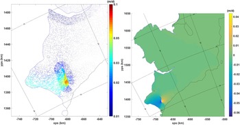
Visual inspection of the MEaSUREs data suggests a number of data artefacts over the BIS and SWGT, and plotting velocity difference vectors between the MEaSUREs and the 2015 Sentinel-1 datasets produces a rather unrealistic spatial pattern of velocity changes (see Fig. 6, left). Although some of the velocity differences seen in the left-hand panel of Figure 6 may be due to real changes in velocities over time, the magnitude and the spatial pattern suggest that most are data errors. We conclude that while the MEaSUREs datasets provided a useful indication of the general spatial pattern of velocities, using that dataset to estimate temporal variations in this area is problematic, and we do not use the MEaSUREs dataset further.
Differences in ice flow velocity as estimated by three different remote-sensing datasets. The three datasets are: (1) velocities from Sentinel-1 images pairs obtained in June 2015 (S), (2) the MEaSUREs dataset from 2007 to 2009 (M), and (3) a dataset derived from RADARSAT-1 data acquired in September–Novrmber 2000 (R). On the left are the velocity differences between the Sentinel-1 2015 and the MEaSUREs 2007–09 datasets (S-M), and on the right are the differences between the Sentinel-1 2015 and the RADARSAT-1 2000 dataset (S-R). Further information about the MEaSUREs and the RADARSAT-1 datasets can be found in Rignot and others (Reference Rignot, Mouginot and Scheuchl2011) and Khazendar and others (Reference Khazendar, Rignot and Larour2009), respectively. The location of HVI in 2008 is shown as a red cross within a red circle.

A comparison between the RADARSAT-1 and Sentinel-1 datasets, from September to November 2000 and June 2015 respectively, resulted in a more coherent and plausible spatial distribution of velocity differences (see Fig. 6, right). Based on the in-situ data discussed above we know that velocities at the HV site decreased from ~2 to ~1.2 m d−1 between 2000 and 2015, or by ~0.8 m d−1 (see Fig. 4). The difference between the 2015 and 2000 speeds shown in Figure 6 at the location of HV is 0.74 m d−1, which compares favourably with the in-situ data. Apart from a few clear artefacts, which show up as individual velocity arrows markedly different from the surrounding ones, we therefore consider the general pattern of velocity differences of these two datasets (Fig. 6, right) to be a reliable indicator of temporal changes in ice flow between 2000 and 2015.
Between 2000 and 2015 there were significant and widespread changes in velocities over both BIS and SWGT (see Fig. 6, right). Generally, flow velocities decreased. The reduction in speed was particularly pronounced over BIS where speeds were reduced by almost a factor of two. This slowdown, seen clearly in the in-situ data from HV, was therefore widespread and not limited to the vicinity of HV alone. The same conclusion was previously drawn by Khazendar and others (Reference Khazendar, Rignot and Larour2009) from a more sparse set of observations.
Furthermore, along the eastern margins of SWGT flow velocities decreased locally by up to 2 m d−1 (see Fig. 6, right). A similarly large change in speed is observed over parts of SWGT directly downstream of the grounding line. Both of these zones contain numerous large open chasms.
3. NUMERICAL MODELLING
As the discussion above has shown, flow velocities on BIS have changed significantly over time. One possible cause for these changes is the growth of the BSC over the last 30 years (see Fig. 1). This growth, documented and discussed in Anderson and others (Reference Anderson, Jones and Gudmundsson2014), may have led to progressive mechanical decoupling between BIS and SWGT and concomitant changes in velocities. Loss of buttressing from MIR leading up to, and following, a calving event in that area in September 1971 (Thomas, Reference Thomas1973b) may also have affected velocities. A further possibility is a more recent growth of the First Chasm (see Fig. 1) towards the north, which started in late 2012 or early 2013, based on satellite imagery.
To quantify these three different scenarios on ice flow, i.e. (a) progressive growth of the BSC, (b) reduction of buttressing stemming from MIR and (c) the recent enlargement of the First Chasm, we use a numerical ice flow model to conduct three corresponding perturbation experiments. We start by initialising the ice flow model using velocities from 2015 obtained from remote sensing and covering the whole of BIS and SWGT. This initialisation procedure is described in more detail in a separate section below. We then perform three numerical perturbation experiments (in the following labelled pBSC, pMIR and pC1) aimed at quantifying the impact of those different scenarios on ice flow.
These three perturbations experiments are:
-
pBSC: Removing BSC. Here the BSC, which has been growing since the early 1980s, is filled in with ice, thereby re-establishing the mechanical contact between BIS and SWGT.
-
pMIR: Removing MIR. Here the ocean bathymetry around MIR is modified so that BIS no longer grounds in that area. The mechanical contact between BIS and MIR is thereby lost.
-
pC1: Removing First Chasm (C1). Here the First Chasm is filled in with ice.
These perturbation experiments are designed to give upper estimates for the possible impacts on ice flow. The BSC has grown steadily for more that 30 years and by removing it we obtain, in an instant, a change in velocity that may have occurred gradually over 30 years. Also, the contact between BIS and MIR may not have been fully lost in the 1971 calving event, and removing all of the contact between BSC and MIR therefore provides an upper bound on the associated loss of buttressing and resulting impact on ice flow. Finally, by healing all of the First Chasm, and filling it with ice of thickness similar to that of the surrounding ice shelf, we arrive at upper limits to the potential impact of C1 on the flow.
3.1. Reference model
Ice flow was modelled using the finite-element ice flow model Úa (Gudmundsson, Reference Gudmundsson2013), employing the shallow ice-shelf approximation (Morland, Reference Morland, van derVeen and Oerlemans1987). This same ice flow approximation was used by Khazendar and others (Reference Khazendar, Rignot and Larour2009), Humbert and others (Reference Humbert2009), and Larour and others (Reference Larour2014), in their previous modelling studies of BIS/SWGT. The numerical model consisted of 121 929 elements ranging in sized from 107 m to 12 km. Linear, quadratic, and cubic triangular elements were used, and the difference in solution used as a measure of discretisation errors.
Flow velocities obtained from Sentinel-1 image pairs acquired on 18 and 30 June 2015, by ENVEO were used to infer rheological parameters of the ice (A), and basal slipperiness (C) over grounded areas within the model domain, using the adjoint capabilities of Úa. The model parameter A relates to the viscous deformability of ice and enters the Glen's flow law, which is a commonly used description of the rheology of glacier ice. The model parameter C enters the Weertman sliding law, which also is a commonly used description of basal processes in numerical ice flow models. Both Glen's flow law and Weertman sliding law are power laws, and here we used the stress exponents n = 3 and m = 3, respectively. The resulting modelled velocity field is shown in the left-hand panel of Figure 7. These modelled velocities agree well with observations as the bivariate histogram of velocity residuals demonstrates in the right-hand panel of Figure 7.
Left: Numerically modelled velocities after model initialisation. Grounding lines are shown as black lines and outer limits of model domain in red. Right: normalised bivariate histogram of velocity residuals. These residuals are the differences between modelled and observed velocities over the whole computational domain where Δu = u modelled − u observed and Δv = v modelled − v observed, and u and v are the x and y components of the surface velocity vector, respectively.

This optimised model uses the ice-shelf geometry and the calving front position from 2015, and it replicates closely the velocities of 2015. We refer to this model as the ‘reference model’. All subsequent perturbation experiments are performed with respect to this reference model.
3.2. Perturbation pBSC: filling in the BSC
We investigate the impact of the progressive enlargement of the BSC over time on ice flow by allowing the chasm to ‘heal’, i.e. by repopulating the chasm with ice. A section of the resulting finite-element mesh around BSC is shown in Figure 8. Note that outside the boundaries of BSC (shown in yellow in Fig. 8) the meshes of both models, i.e. the one used in the perturbation experiment and that of the reference model, are identical. When comparing velocities between these model runs, there was therefore no need for an interpolation of any computed fields between different finite-element meshes.
Sections of the finite-element meshes used in the perturbation experiments pBSC (left) and the pC1 (right). The figure to the left shows how the BSC has been filled in. The yellow line marks the outlines of the BSC in 2015. The elements inside of this polygon were added to the reference model. Outside of the yellow polygon, the mesh is identical to that of the reference model. The figure to the right shows similarly how the First Chasm (C1) has been filled in. The thick red lines mark the boundaries of the chasm in 2015. Outside of this boundary, the mesh of is identical to that of the reference model.

The rheological parameters of the ice within the infill were set identical to those of the surrounding ice. Flow velocities were then re-calculated and compared with that of the reference model. The resulting velocity differences are shown in Figure 9, left. The velocity arrows in Figure 9, left, are calculated as
 $$\Delta v_{{\rm pBSC}} = v_{{\rm NoBSC}} - v_{{\rm ReferenceModel}}$$
Perturbations in velocity (left) and speed (right) perturbations for the pBSC experiment. The velocities shown are the differences between modelled velocities with BS filled in and those of the reference model. Similarly, the speeds (right) are the differences in modelled speed with and without the BSC.

As Figure 9 shows, the creation of BSC has a much greater impact on SWGT than on BIS. Over large sections of SWGT the perturbation in velocities ranges from ~0.5 to 1.0 m d−1, whereas over BIS they are everywhere <~0.2 m d−1. Even accounting for the generally larger velocities on SWGT (see Fig. 7, left), the relative change in velocities on SWGT caused by the growth of BSC is larger over SWGT than over BIS.
The velocity perturbations (see Fig. 9) are mostly transverse to the flow field of the reference model, i.e. with respect to the 2015 flow field. This suggests that as BSC grew, flow directions changed away from the chasm. As a consequence, across SWGT velocities may have shifted somewhat towards the east, while on BIS the shift in flow direction will have been towards the west.
3.3. Perturbation pMIR: removing the MIR
In a second perturbation experiment we remove any contact between BIS and MIR. This was done by lowering the sea floor in the area sufficiently for contact between the ice and the ocean floor to be lost. The resulting velocity perturbations, defined as,
 $$\Delta v_{{\rm pMIR}} = v_{{\rm NoMIR}} - v_{{\rm ReferenceModel}}$$
and changes in speed are shown in Figure 10.
Perturbations in velocity (left) and the speed (right) for the pMIR experiment. The velocities shown are the differences between modelled velocities with any contact between the ice shelf and MIR removed and those of the reference model. Similarly, the perturbed speeds (right) are the differences in modelled speed with and without MIR. Contact between the ice shelf and MIR was removed by lowering the ocean bathymetry below the draft of the ice shelf in that area.

As mentioned above, our description of glacier flow is based on the shallow-ice shelf approximation. For this reason our numerical model is not able to describe any potential ice-shelf flexure around MIR. However, all horizontal stress gradients are included in our numerical model, and for that reason we expect the model to be able to adequately describe the impact of MIR on the horizontal stress balance within the ice shelf.
Removing MIR causes an almost twofold increase in velocities over a large section of the BIS. The ice thickness around MIR is of the order of 100 m, but velocities chance by more than 10% over distances of up to 40 km. The impact on the velocity field is, thus, felt widely over BIS and not only limited to an area of a few mean ice thicknesses from MIR. The perturbation in velocity is approximately aligned with the unperturbed flow regime, i.e. that of the reference model corresponding to year 2015 (Fig. 7). While the loss of buttressing provided by MIR is found to have a decisive impact on the velocity distribution of BIS, the impact on velocities over SWGT is modest or on the order of 0.1 m d−1.
3.4. Perturbation pC1: filling in the First Chasm
In our final perturbation experiment we repopulate the First Chasm (C1) with ice to inspect the potential impact of this structure on the flow field. In the reference run, C1 was modelled as an ice free area, i.e. as a gap within the ice shelf. In reality the C1 is filled with a few meter thick multi-year sea ice. In the perturbation experiment, C1 is filled in with ice of same thickness as the surrounding ice. Hence, our perturbation experiment almost certainly provides an upper estimate of the potential impact of C1 on the flow field of BIS.
The First (C1) and the Second Chasms (C2) are prominent features of BIS. Our inspection of available satellite imagery shows them to have been formed sometime between 1973 and 1985. Most likely they were initially formed close to the grounding line, and sometime shortly after 1973. They appear to have been inactive for most of this time, but in late 2012 satellite images showed that the First Chasm had been reactivated and started to grow towards the north.
The perturbations in velocities and changes in flow speeds following an in-filling of C1 are shown in Figure 11. As in the other perturbation experiments, the velocity perturbations were defined with respect to the reference model as
 $$\Delta v_{{\rm pC1}} = v_{{\rm NoC1}} - v_{{\rm ReferenceModel}}$$
Perturbations in velocity (left) and speed (right) for the pC1 experiment. In this experiment the First Chasm has been repopulated with ice and the differences in velocities (left) and speeds (right) without and with the First Chasm are shown. Filling in the First Chasm causes a decrease in speed downstream and increase in speed upstream of it.
As Figure 11 shows, the changes in velocities are quite modest, in the order of a few centimetres per day as whereas typical current velocities on BIS are ~1 m d−1. The change in velocity is limited to the BIS alone. Flow speeds decrease downstream of C1 in response to the filling-in of C1, and increase upstream. Note that, because in the perturbation experiment C1 is filled with ice, the recently renewed growth and reactivation of C1 will impact the flow field in an opposite manner from that shown in Figure 11.
4. DISCUSSION
Comparison of Figures 9, 10 shows that removing contact with MIR has a much greater impact on the velocities on BIS than the creation of the BSC. Although the growth of BSC does affect ice flow, the effect is mostly limited to SWGT and the suture zone between BIS and SWGT. Loss of contact between MIR and BIS, on the other hand, causes a doubling in ice velocities over most of BIS. Furthermore, the reactivation of C1 (see Fig. 11) leads only to a modest increase in velocities downstream of C1. Hence, of the perturbations experiments described above, only the loss of a contact between BIS and MIR is found to be able to produce change in velocities across the BIS of a magnitude similar to that observed.
The perturbations experiments therefore demonstrate that although the progressive enlargement of BSC and the reactivation of C1 with time may have had some effect on flow of BIS, these cannot be the main drivers for the observed changes. An explanation supported by the numerical experiments, however, is the possibility that the 1971 calving event around BIS led to a loss of contact with the BIS and an increase in ice flow speed, and that velocities went back to previous levels as this contact was re-established. The general pattern of temporal velocity variations (see Fig. 5), with a sharp increase in velocities at ~1971, a continued gentle rate of increase until 1997, followed by a twofold decrease between 1997 and 2012, does fit this explanation. The implication is that a degree in contact between MIR and BIS, required to cause a significant reduction in flow speed, was only established at ~1997, i.e. ~26 years after the calving event took place. After 1997, the increase in buttressing provided by MIR then continued to cause a decrease in BIS flow velocities until 2012.
The period from 1971 to 1997 may at first appear to be a somewhat long time interval for re-establishing full contact between BIS and MIR. Ice velocities upstream of MIR were most likely somewhere between 400 and 700 m a−1 in that period, and the ice will therefore have travelled a distance of at least 10 km. However, aerial imagery shown in Figure 12 indicates that it may indeed have taken this long for the ice distribution around MIR to reach a similar state to that prior to the 1971 calving event. Comparing aerial photographs taken in 1967, or ~4 years prior to the calving event, to similar photographs taken in 2003, a few years after the velocities started to slow down again, shows a greater number of pressure ridges around MIR in 1967 than in 2003 (see Fig. 12). This suggests that in 2003 the contact between MIR and BIS was still not as well established as it was in 1967. It is only more recently that the number of pressure ridges around MIR has become comparable with that of 1967, consistent with the fact that velocities continued to slow down after 2003.
Aerial photographs showing the MIR in 1967 (left) and 2003 (right).

As the modelling exercises described above showed, the filling-in of C1 produces a decrease in velocities downstream and a concomitant upstream increase in velocities. A recent weakening of First Chasm therefore provides a possible explanation for the increase in velocities observed at site HV (located downstream of C1) to have started in late 2012. However, perturbation experiment pC1 also suggests that the observed rate of change is too large to be only due to the growth of C1. The cause for the latest increase in flow velocities therefore remains unclear. Possibly, the recently observed enlargement of C1 is only a small part of much bigger ongoing changes in the area such as weakening of C2 and reduction in ice strength through accumulated damage. Without direct velocity observations in the area we lack the data to test this hypothesis.
The results of our perturbations experiments are in good general agreement with previous results obtained by Khazendar and others (Reference Khazendar, Rignot and Larour2009). Using a methodology similar to ours, Khazendar and others (Reference Khazendar, Rignot and Larour2009) studied the impact of an enlargement of the BSC on ice flow. They concluded, as do we, that the resulting impact of flow velocities is greater over SWGT than over BIS. While the spatial pattern of speed change is similar (compare Fig. 6 in Khazendar and others (Reference Khazendar, Rignot and Larour2009) with Fig. 9) the magnitude and direction of the perturbed velocity field are somewhat different. These differences are most likely due to different geometries for the BSC used in this study as compared with that of Khazendar and others (Reference Khazendar, Rignot and Larour2009). Here the BSC geometry is that of 2015, whereas the geometry in Khazendar and others (Reference Khazendar, Rignot and Larour2009) appears to be that of 2008. It is therefore not surprising that our numbers for the effect of BSC on ice flow are somewhat larger.
Although not described here, we did conduct further perturbations experiments involving ice weakening around rift structures on SWGT, and over the ice mélange area between BIS and SWGT. Similar to Khazendar and others (Reference Khazendar, Rignot and Larour2009) we found this to affect velocities on both BIS and SWGT. While we do not exclude the possibility that such changes in ice rheology may play a role in explaining historical flow variations on BIS and SWGT, we consider changes in mechanical interactions between BIS and MIR to be a more likely mechanism. We arrive at this conclusion by noticing, firstly, that loss of contact between BIS and MIR has the potential to explain both the observed increase and the decrease in speed over time. Secondly, in an agreement with observations from remote-sensing data (see Fig. 6), it provides an explanation for why the changes in velocities between 2000 and 2015 were greater over BIS than over SWGT. Had the changes been caused by modification in (effective) ice rheology, as advocated by Khazendar and others (Reference Khazendar, Rignot and Larour2009), velocities over SWGT and BIS would have been affected in about equal measures (see Fig. 5 in Khazendar and others, Reference Khazendar, Rignot and Larour2009). Further, to explain both the observed increase and later decrease in velocities through changes in ice rheology, requires corresponding temporal changes in ice rheology for which there is no direct evidence. On the other hand, explaining the changes through a loss and subsequent gradual regaining of contact between MIR and BIS does not require such an assumption of temporal changes in ice properties, explains both the increase as well as the decrease in speed, and produces, in full accordance with observations, a larger change in velocity over BIS than over SWGT.
Khazendar and others (Reference Khazendar, Rignot and Larour2009) did not perform a perturbation experiment comparable with our pMIR experiment. However, they state that effects of changing interactions between BIS and MIR would be local, and therefore discount that as a possible explanation for the 1970s acceleration. Our perturbation experiment (pMIR) on the other hand suggests that the effect is large (i.e. twofold increase in velocity) and widely felt over the whole of BIS. The main argument that Khazendar and others (Reference Khazendar, Rignot and Larour2009) raise against changes in contact between BIS and MIR being responsible is the observed area-wide increase in velocities over both BIS and SWGT. At the time of their study the number of velocity data points was limited and no area-wide information on velocity change was available. Furthermore, the fact that velocities started to decrease at ~1997, or shortly thereafter, had not been published at the time of their study. Hence, the primary observations that were used to formulate our alternative explanation were not available to Khazendar and others (Reference Khazendar, Rignot and Larour2009) when their study was conducted.
A number of velocity changes seen in the remote-sensing data (Fig. 6, right) are, however, clearly not related to varying interaction between BIS and MIR. Two such areas (in the following labelled 1 and 4 for reasons that will become clear) of velocity change are: (1) the eastern margin of SWGT, and (4) the southern limits of SWGT ~30 km downstream of the grounding line. Between 2000 and 2015 velocities changed by ~1.5 m d−1 over both of these areas. These two rift structures were labelled as rifts 1 and 4 by Larour and others (Reference Larour2014), hence our labelling scheme, who explicitly included them as open chasms in their ice flow modelling study. As shown by Larour and others (Reference Larour2014) this suggests that changes in widths and lengths of those rifts may be the reason for the observed variations in velocity over those areas.
5. CONCLUSIONS AND OUTLOOK
We have presented and analysed a 55-year long time series of velocity changes on the BIS. To our knowledge, this is the longest time series of this type from any ice shelf. The data show significant variations in flow speeds over time, with a twofold increase in speed at BIS ~1970, followed by a decrease back to pre-1970 speeds by 2012, after which a renewed period of acceleration started. Over the whole observational period velocities have changed frequently at a rate of ~10% a−1.
Through a number of perturbations experiments performed using a numerical ice flow model, we have been able to identify changes in the mechanical connection between MIR and BIS following a calving event in 1971 as a possible reason for the increase and subsequent decrease in velocities. Comparison of two velocity maps from 2000 and 2015, both derived from remote-sensing data, shows a greater reduction in ice velocities over BIS than SWGT, and the observed spatial pattern of velocity change closely matches the numerically modelled impact of MIR on ice flow.
The main features of the temporal and the spatial variability in velocities can be explained as follows: In 1971 a loss in buttressing following the calving event around MIR caused an almost instantaneous twofold increase in ice velocity over large sections of BIS. After the calving event, contact between MIR and BIS was gradually re-established. Around 1997, contact was again sufficiently strong to start to affect velocities significantly, and a period of rapid deceleration started, which continued until 2012 (see Fig. 13).
Velocity changes with time at BIS. The green line is a simplified version of velocity changes up to 2000. As argued in the text, the velocity increase in 1971 can be explained as a consequence reduction in buttressing following the 1971 calving event around MIR. The slow down starting at ~1997 may be caused be the contact between MIR and BIS slowly being re-established, while the more recent increase in speed starting in late 2012 could at least in parts be due to the reactivation of First Chasm.

Not all of the observed variability may be explicable in this manner. In particular, the new phase of acceleration starting in 2012 is presumably due to some other cause. The recent re-activation of First Chasm is a possibly explanation, but numerical perturbation experiments suggest that the effect on ice flow is too small. Possibly the weakening is not limited to First Chasm alone, or alternatively, some other mechanism is responsible for this most recent phase of velocity change on BIS. This recent phase of a sharp increase in ice speeds on BIS is here not explained, and further studies are required.
ACKNOWLEDGEMENTS
We thank the reviewers for their reviews and insightful and detailed comments. Processing of Sentinel-1 ice velocity maps by ENVEO was supported by the Austrian Space Applications Programme/Austrian Research Promotion Agency (FFG) and the ESA Antarctic ice sheet CCI project. Copernicus Sentinel-1 data were made available through ESA Sentinel Scientific Data Hub. G.H.G. and J.D.R. were partly supported as part of the Polar Science for Planet Earth funding from the Natural Environment Research Council (NERC) to the British Antarctic Survey.


 Open access