


1 Introduction
Let G be a connected semi-simple algebraic group over $\mathbb {Q}$
[Reference MilneMil18], [Reference Borel and TitsBT65] and let
$\mathbb {Q}$
[Reference MilneMil18], [Reference Borel and TitsBT65] and let $G_\infty :=G(\mathbb {R})$
be the group of real points of G. Let
$G_\infty :=G(\mathbb {R})$
be the group of real points of G. Let $\Gamma \subset G(\mathbb {Q})$
be an arithmetic subgroup. Then
$\Gamma \subset G(\mathbb {Q})$
be an arithmetic subgroup. Then $\Gamma $
is a lattice in
$\Gamma $
is a lattice in $G_\infty $
. Let
$G_\infty $
. Let $\rho \colon G\to \operatorname {GL}(V)$
be a rational finite-dimensional complex representation. Suppose that there is a
$\rho \colon G\to \operatorname {GL}(V)$
be a rational finite-dimensional complex representation. Suppose that there is a $\Gamma $
-invariant lattice
$\Gamma $
-invariant lattice $L\subset V$
with
$L\subset V$
with $L\otimes _{\mathbb {Z}}\mathbb {C}=V$
. The cohomology groups
$L\otimes _{\mathbb {Z}}\mathbb {C}=V$
. The cohomology groups $H^j(\Gamma ;L)$
are finitely generated abelian groups. Let
$H^j(\Gamma ;L)$
are finitely generated abelian groups. Let $H^j(\Gamma ;L)_{\operatorname {free}}$
and
$H^j(\Gamma ;L)_{\operatorname {free}}$
and $H^j(\Gamma ;L)_{\operatorname {tor}}$
be the free and the torsion subgroups, respectively. We have
$H^j(\Gamma ;L)_{\operatorname {tor}}$
be the free and the torsion subgroups, respectively. We have $H^j(\Gamma ;L)_{\operatorname {free}}\otimes _{\mathbb {Z}}\mathbb {C}\cong H^j(\Gamma ;V)$
. If the underlying locally symmetric space has an algebro-geometric structure, the Langlands conjectures predict that there are deep connections between the cohomology groups
$H^j(\Gamma ;L)_{\operatorname {free}}\otimes _{\mathbb {Z}}\mathbb {C}\cong H^j(\Gamma ;V)$
. If the underlying locally symmetric space has an algebro-geometric structure, the Langlands conjectures predict that there are deep connections between the cohomology groups $H^j(\Gamma ;V)$
and the theory of automorphic forms and number theory. Recent results show that torsion classes are also connected to number theory. Ash [Reference AshAsh92] conjectured that for a congruence subgroup
$H^j(\Gamma ;V)$
and the theory of automorphic forms and number theory. Recent results show that torsion classes are also connected to number theory. Ash [Reference AshAsh92] conjectured that for a congruence subgroup $\Gamma \subset \operatorname {SL}(n,\mathbb {Z})$
, any Hecke eigenclass
$\Gamma \subset \operatorname {SL}(n,\mathbb {Z})$
, any Hecke eigenclass $\xi \in H^\ast (\Gamma ;\mathbb {F}_p)$
is attached to a continuous semisimple Galois representation
$\xi \in H^\ast (\Gamma ;\mathbb {F}_p)$
is attached to a continuous semisimple Galois representation $\rho \colon \operatorname {Gal}(\bar {\mathbb {Q}}/\mathbb {Q})\to \operatorname {GL}(n,\mathbb {F}_p)$
such that Frobenius and Hecke eigenvalues match up. A more general version of this conjecture has been proved by Scholze [Reference ScholzeSch15]. However, much less is known about the structure of the torsion group, for example, its size. If G is
$\rho \colon \operatorname {Gal}(\bar {\mathbb {Q}}/\mathbb {Q})\to \operatorname {GL}(n,\mathbb {F}_p)$
such that Frobenius and Hecke eigenvalues match up. A more general version of this conjecture has been proved by Scholze [Reference ScholzeSch15]. However, much less is known about the structure of the torsion group, for example, its size. If G is $\mathbb {Q}$
-anisotropic, i.e.,
$\mathbb {Q}$
-anisotropic, i.e., $\Gamma \backslash G_\infty $
is compact, Bergeron and Venkatesh [Reference Bergeron and VenkateshBV13] obtained first results concerning the growth of torsion, if
$\Gamma \backslash G_\infty $
is compact, Bergeron and Venkatesh [Reference Bergeron and VenkateshBV13] obtained first results concerning the growth of torsion, if $\Gamma $
varies in a tower of lattices, and they also formulated a conjecture predicting the growth of torsion in general.
$\Gamma $
varies in a tower of lattices, and they also formulated a conjecture predicting the growth of torsion in general.
To state the results and the conjecture we need to introduce some notation. Let $K\subset G_\infty $
be a maximal compact subgroup. Let
$K\subset G_\infty $
be a maximal compact subgroup. Let $\widetilde X =G_\infty /K$
be the associated global Riemannian symmetric space. Let
$\widetilde X =G_\infty /K$
be the associated global Riemannian symmetric space. Let ${\mathfrak g}$
and
${\mathfrak g}$
and ${\mathfrak k}$
be the Lie algebras of
${\mathfrak k}$
be the Lie algebras of $G_\infty $
and K, respectively. The fundamental rank
$G_\infty $
and K, respectively. The fundamental rank $\delta (G)$
of G is defined by
$\delta (G)$
of G is defined by $\delta (G):=\operatorname {rank}({\mathfrak g}_{\mathbb {C}})-\operatorname {rank}({\mathfrak k}_{\mathbb {C}})$
. As explained by Bergeron and Venkatesh [Reference Bergeron and VenkateshBV13], when
$\delta (G):=\operatorname {rank}({\mathfrak g}_{\mathbb {C}})-\operatorname {rank}({\mathfrak k}_{\mathbb {C}})$
. As explained by Bergeron and Venkatesh [Reference Bergeron and VenkateshBV13], when $\delta (G)=1$
, one expects for arithmetic reasons that
$\delta (G)=1$
, one expects for arithmetic reasons that $H^\ast (\Gamma ;L)$
should have a lot of torsion and a small free part. This conjecture is supported by the following result proved in [Reference Bergeron and VenkateshBV13] for anisotropic G. Assume that
$H^\ast (\Gamma ;L)$
should have a lot of torsion and a small free part. This conjecture is supported by the following result proved in [Reference Bergeron and VenkateshBV13] for anisotropic G. Assume that $\cdots \subset \Gamma _j\subset \Gamma _{j-1}\subset \cdots \subset \Gamma $
is a decreasing sequence of congruence subgroups such that
$\cdots \subset \Gamma _j\subset \Gamma _{j-1}\subset \cdots \subset \Gamma $
is a decreasing sequence of congruence subgroups such that $\cap _j\Gamma _j=\{1\}$
. L is called strongly acyclic for the family
$\cap _j\Gamma _j=\{1\}$
. L is called strongly acyclic for the family $\{\Gamma _j\}$
if the Laplacians on V-valued i-forms on
$\{\Gamma _j\}$
if the Laplacians on V-valued i-forms on $\Gamma _k\backslash \widetilde X$
are uniformly bounded away from 0 for all degrees i and all
$\Gamma _k\backslash \widetilde X$
are uniformly bounded away from 0 for all degrees i and all $\Gamma _k$
. In this case,
$\Gamma _k$
. In this case, $H^\ast (\Gamma _k\setminus \widetilde {X};L)$
is a pure torsion group. If
$H^\ast (\Gamma _k\setminus \widetilde {X};L)$
is a pure torsion group. If $\delta (G)=1$
, then by [Reference Bergeron and VenkateshBV13, Theorem 1.4] one has
$\delta (G)=1$
, then by [Reference Bergeron and VenkateshBV13, Theorem 1.4] one has
 $$ \begin{align} \liminf_{j\to\infty}\sum_q\frac{\log|H^q(\Gamma_j;L)_{\operatorname{tor}}|}{[\Gamma\colon\Gamma_j]}\ge c_{G,L}\operatorname{vol}(\Gamma\backslash\widetilde X)>0, \end{align} $$
where the sum is over the integers q such that $q+\frac {\dim (\widetilde X)+1}{2}$
is odd and
$q+\frac {\dim (\widetilde X)+1}{2}$
is odd and $c_{G,L}>0$
is a constant that depends only on G and L. To establish the lower bound, Bergeron and Venkatesh prove the following result
$c_{G,L}>0$
is a constant that depends only on G and L. To establish the lower bound, Bergeron and Venkatesh prove the following result
 $$ \begin{align} \lim_{j\to\infty}\sum_q(-1)^{q+\frac{\dim (\widetilde X)+1}{2}}\frac{\log|H^q(\Gamma_j;L)_{\operatorname{tor}}|} {[\Gamma\colon\Gamma_j]}=c_{G,L}\operatorname{vol}(\Gamma\backslash\widetilde X). \end{align} $$
The proof of (1.2) uses the equality of analytic torsion and Reidemeister torsion. It follows from (1.1) that for some q, $|H^q(\Gamma _j;L)_{\operatorname {tor}}|$
grows exponentially as
$|H^q(\Gamma _j;L)_{\operatorname {tor}}|$
grows exponentially as $j\to \infty $
. Based on (1.2), Bergeron and Venkatesh made a conjecture with a precise prediction of the growth of torsion [Reference Bergeron and VenkateshBV13, Conjecture 1.3] without any assumption on L. The conjecture states that for each q
$j\to \infty $
. Based on (1.2), Bergeron and Venkatesh made a conjecture with a precise prediction of the growth of torsion [Reference Bergeron and VenkateshBV13, Conjecture 1.3] without any assumption on L. The conjecture states that for each q
 $$ \begin{align} \lim_{j\to\infty}\frac{\log|H^q(\Gamma_j;L)_{\operatorname{tor}}|}{[\Gamma\colon\Gamma_j]} \end{align} $$
exists and equals zero unless $\delta (G)=1$
and
$\delta (G)=1$
and $q=\frac {\dim (\widetilde X)+1}{2}$
. In this case it equals
$q=\frac {\dim (\widetilde X)+1}{2}$
. In this case it equals $c_{G,L}\operatorname {vol}(\Gamma \backslash \widetilde X)$
with
$c_{G,L}\operatorname {vol}(\Gamma \backslash \widetilde X)$
with $c_{G,L}>0$
. All this is under the assumption that the
$c_{G,L}>0$
. All this is under the assumption that the $\mathbb {Q}$
-rank of G is 0.
$\mathbb {Q}$
-rank of G is 0.
Since many important arithmetic groups are not co-compact, it is desirable to extend these results to groups G with $\mathbb {Q}$
-rank
$\mathbb {Q}$
-rank $>0$
. In [Reference Ash, Gunnells, McConnell and YasakiAGMY20] the authors made comprehensive computations of torsion subgroups in
$>0$
. In [Reference Ash, Gunnells, McConnell and YasakiAGMY20] the authors made comprehensive computations of torsion subgroups in $H^j(\Gamma ,\mathbb {Z})$
, where
$H^j(\Gamma ,\mathbb {Z})$
, where $\Gamma \subset G(\mathbb {Q})$
is an arithmetic subgroup for
$\Gamma \subset G(\mathbb {Q})$
is an arithmetic subgroup for $G=\operatorname {GL}_n/\mathbb {Q}$
,
$G=\operatorname {GL}_n/\mathbb {Q}$
, $n=3,4,5$
, or
$n=3,4,5$
, or $G=\operatorname {GL}_2$
over specific number fields for which
$G=\operatorname {GL}_2$
over specific number fields for which $\delta (G)=1$
or
$\delta (G)=1$
or $2$
. They use their computations to extend the conjecture (1.3) of Bergeron und Venkatesh by removing the restriction to the cocompact case and allowing any growth of level, not just in a tower. These are Conjectures 7.1 and 7.2 in [Reference Ash, Gunnells, McConnell and YasakiAGMY20]. In particular, Conjecture 7.2 predicts that for a family
$2$
. They use their computations to extend the conjecture (1.3) of Bergeron und Venkatesh by removing the restriction to the cocompact case and allowing any growth of level, not just in a tower. These are Conjectures 7.1 and 7.2 in [Reference Ash, Gunnells, McConnell and YasakiAGMY20]. In particular, Conjecture 7.2 predicts that for a family $\{\Gamma _j\}_{j\in \mathbb {N}}$
of congruence subgroups in a fixed arithmetic groups
$\{\Gamma _j\}_{j\in \mathbb {N}}$
of congruence subgroups in a fixed arithmetic groups $\Gamma $
with
$\Gamma $
with $\operatorname {level}(\Gamma _j)\to \infty $
,
$\operatorname {level}(\Gamma _j)\to \infty $
,
 $$ \begin{align} \liminf_{j\to \infty}\frac{\log|H^q(\Gamma_j;L)_{\operatorname{tor}}|}{[\Gamma\colon\Gamma_j]} \end{align} $$
exists. If G has $\mathbb {Q}$
-rank
$\mathbb {Q}$
-rank $>0$
, then the lim-inf equals zero unless
$>0$
, then the lim-inf equals zero unless $\delta (G)=1$
and q is the top degree of the cuspidal range.
$\delta (G)=1$
and q is the top degree of the cuspidal range.
The first step beyond $\mathbb {Q}$
-rank 0 is the case of hyperbolic manifolds of finite volume which has been treated in [Reference PfaffPfa14], [Reference Müller and RochonMR21]. This is the
$\mathbb {Q}$
-rank 0 is the case of hyperbolic manifolds of finite volume which has been treated in [Reference PfaffPfa14], [Reference Müller and RochonMR21]. This is the $\mathbb {R}$
-rank 1 case. The method of [Reference Bergeron and VenkateshBV13] is based on the equality of analytic torsion and Reidemeister torsion [Reference CheegerChe79], [Reference MüllerMül78], [Reference MüllerMül93]. This equality is not available in the non-compact case. However, for hyperbolic manifolds of finite volume there is a formula with an explicit defect term [Reference Müller and RochonMR20], whose asymptotic behaviour can be controlled for a family of congruence subgroups
$\mathbb {R}$
-rank 1 case. The method of [Reference Bergeron and VenkateshBV13] is based on the equality of analytic torsion and Reidemeister torsion [Reference CheegerChe79], [Reference MüllerMül78], [Reference MüllerMül93]. This equality is not available in the non-compact case. However, for hyperbolic manifolds of finite volume there is a formula with an explicit defect term [Reference Müller and RochonMR20], whose asymptotic behaviour can be controlled for a family of congruence subgroups $\{\Gamma _j\}_{j\in \mathbb {N}}$
of a fixed arithmetic group
$\{\Gamma _j\}_{j\in \mathbb {N}}$
of a fixed arithmetic group $\Gamma $
. There is another obstacle if one wants to apply the result to deduce a formula similar to (1.2). Even if L strongly acyclic, the cohomology
$\Gamma $
. There is another obstacle if one wants to apply the result to deduce a formula similar to (1.2). Even if L strongly acyclic, the cohomology $H^\ast (\Gamma ;L\otimes \mathbb {C})$
does not vanish. Only the interior cohomology vanishes. In general, there is cohomology coming from the boundary of the Borel-Serre compactification. This is the Eisenstein cohomology which gives rise to a non-trivial regulator in the expression of the Reidemeister torsion in terms of the order of the torsion subgroup in the cohomology
$H^\ast (\Gamma ;L\otimes \mathbb {C})$
does not vanish. Only the interior cohomology vanishes. In general, there is cohomology coming from the boundary of the Borel-Serre compactification. This is the Eisenstein cohomology which gives rise to a non-trivial regulator in the expression of the Reidemeister torsion in terms of the order of the torsion subgroup in the cohomology $H^\ast (\Gamma ;L)$
[Reference Bergeron and VenkateshBV13,
$H^\ast (\Gamma ;L)$
[Reference Bergeron and VenkateshBV13, $\S$
2]. We were able to cope with these problems and established a lower bound similar to (1.1) [Reference Müller and RochonMR21].
$\S$
2]. We were able to cope with these problems and established a lower bound similar to (1.1) [Reference Müller and RochonMR21].
In this paper we consider $\mathbb {Q}$
-rank 1 cases with
$\mathbb {Q}$
-rank 1 cases with $\mathbb {R}$
-rank
$\mathbb {R}$
-rank $>1$
. The corresponding locally symmetric space is a manifold with fibred cusps. The semi-simple group G is defined as follows. Let F be a number field of degree
$>1$
. The corresponding locally symmetric space is a manifold with fibred cusps. The semi-simple group G is defined as follows. Let F be a number field of degree $d_{F}$
over
$d_{F}$
over $\mathbb {Q}$
. Let
$\mathbb {Q}$
. Let $\mathcal {O}_{F}$
denote the ring of algebraic integers of F. We consider
$\mathcal {O}_{F}$
denote the ring of algebraic integers of F. We consider $\operatorname {SL}(2)$
as an algebraic group over F. Let
$\operatorname {SL}(2)$
as an algebraic group over F. Let $G_0=\operatorname {SL}(2)/F$
and let
$G_0=\operatorname {SL}(2)/F$
and let
 $$ \begin{align} G=\operatorname{Res}_{F/\mathbb{Q}}(G_0) \end{align} $$
be the algebraic group, which is obtained from $G_0$
by restriction of scalars [Reference WeilWei82]. Then G is a semi-simple algebraic group over
$G_0$
by restriction of scalars [Reference WeilWei82]. Then G is a semi-simple algebraic group over $\mathbb {Q}$
. Moreover, we have
$\mathbb {Q}$
. Moreover, we have
 $$\begin{align*}G_\infty=G(\mathbb{R})=\prod_{v|\infty} \operatorname{SL}(2,F_v),\quad G(\mathbb{Q})=\operatorname{SL}(2,F). \end{align*}$$
Let $\sigma _1,\ldots , \sigma _{r_1}$
be the embeddings of F in
$\sigma _1,\ldots , \sigma _{r_1}$
be the embeddings of F in $\mathbb {R}$
and let
$\mathbb {R}$
and let $\tau _1,\overline {\tau }_1,\ldots ,\tau _{r_2},\overline {\tau }_{r_2}$
denote the remaining embeddings of F in
$\tau _1,\overline {\tau }_1,\ldots ,\tau _{r_2},\overline {\tau }_{r_2}$
denote the remaining embeddings of F in $\mathbb {C}$
, so that
$\mathbb {C}$
, so that $d_{F}=r_1+2r_2$
. Then
$d_{F}=r_1+2r_2$
. Then
 $$ \begin{align*}G_{\infty}= \operatorname{SL}(2,F\otimes_{\mathbb{Q}}\mathbb{R})= \operatorname{SL}(2,\mathbb{R})^{r_1}\times \operatorname{SL}(2,\mathbb{C})^{r_2} \end{align*} $$
and $K_\infty =\operatorname {SO}(2)^{r_1}\times \operatorname {SU}(2)^{r_2}$
is a maximal compact subgroup. The corresponding symmetric space equals
$K_\infty =\operatorname {SO}(2)^{r_1}\times \operatorname {SU}(2)^{r_2}$
is a maximal compact subgroup. The corresponding symmetric space equals
 $$ \begin{align*}\widetilde{X}:= G_{\infty}/K_\infty= (\mathbb{H}^2)^{r_1}\times (\mathbb{H}^3)^{r_2}. \end{align*} $$
Let $\Gamma \subset \operatorname {SL}(2,\mathcal {O}_{F})$
be a torsion free subgroup of finite index. Then
$\Gamma \subset \operatorname {SL}(2,\mathcal {O}_{F})$
be a torsion free subgroup of finite index. Then $\Gamma $
is a discrete subgroup of
$\Gamma $
is a discrete subgroup of $G_{\infty }$
via the embedding
$G_{\infty }$
via the embedding $\iota : \Gamma \to \operatorname {SL}(2,\mathbb {R})^{r_1}\times \operatorname {SL}(2,\mathbb {C})^{r_2}$
defined by
$\iota : \Gamma \to \operatorname {SL}(2,\mathbb {R})^{r_1}\times \operatorname {SL}(2,\mathbb {C})^{r_2}$
defined by
 $$ \begin{align} & \left( \begin{array}{@{}cc@{}} \alpha & \beta \\ \gamma & \delta \end{array} \right)\mapsto \nonumber \\ &\left(\left( \begin{array}{@{}cc@{}} \sigma_1(\alpha) & \sigma_1(\beta) \\ \sigma_1(\gamma) & \sigma_1(\delta) \end{array} \right),\ldots, \left( \begin{array}{@{}cc@{}} \sigma_{r_1}(\alpha) & \sigma_{r_1}(\beta) \\ \sigma_{r_1}(\gamma) & \sigma_{r_1}(\delta) \end{array} \right), \left( \begin{array}{@{}cc@{}} \tau_1(\alpha) & \tau_1(\beta) \\ \tau_1(\gamma) & \tau_1(\delta) \end{array} \right), \ldots, \left( \begin{array}{@{}cc@{}} \tau_{r_2}(\alpha) & \tau_{r_2}(\beta) \\ \tau_{r_2}(\gamma) & \tau_{r_2}(\delta) \end{array} \right)\right) \end{align} $$
and the quotient
 $$ \begin{align*}X= \Gamma\setminus \widetilde{X} \end{align*} $$
is a manifold. As described in [Reference BorelBor74], it comes with a natural metric. First, the invariant metric one should consider on $\widetilde {X}=(\mathbb {H}^2)^{r_1}\times (\mathbb {H}^3)^{r_2}$
is
$\widetilde {X}=(\mathbb {H}^2)^{r_1}\times (\mathbb {H}^3)^{r_2}$
is
 $$ \begin{align} \widetilde{g}= \sum_{i=1}^{r_1}\frac{dx_i^2+ dy_i^2}{y_i^2}+ 2 \sum_{j=1}^{r_2} \frac{|dz_j|^2+ dt_j^2}{t_j^2} \end{align} $$
using the upper half-plane and the upper half-space models for $\mathbb {H}^2$
and
$\mathbb {H}^2$
and $\mathbb {H}^3$
. Since
$\mathbb {H}^3$
. Since $\Gamma $
acts by isometries,
$\Gamma $
acts by isometries, $\widetilde {g}$
descends to a metric g on X. The manifold X has the homotopy type of a compact manifold with boundary with each boundary component corresponding to a fibred cusp end. If
$\widetilde {g}$
descends to a metric g on X. The manifold X has the homotopy type of a compact manifold with boundary with each boundary component corresponding to a fibred cusp end. If $\mathbb {P}^1(F)$
is the projective line of the number field F, then the fibred cusp ends are in bijection with
$\mathbb {P}^1(F)$
is the projective line of the number field F, then the fibred cusp ends are in bijection with $\Gamma \setminus \mathbb {P}^1(F)$
. Let in fact
$\Gamma \setminus \mathbb {P}^1(F)$
. Let in fact $\mathfrak {P}_{\Gamma }\subset \mathbb {P}^1(F)$
be a set of representatives for the classes in
$\mathfrak {P}_{\Gamma }\subset \mathbb {P}^1(F)$
be a set of representatives for the classes in $\Gamma \setminus \mathbb {P}^1(F)$
, so that
$\Gamma \setminus \mathbb {P}^1(F)$
, so that $\mathfrak {P}_{\Gamma }$
naturally corresponds to the set of fibred cusp ends of X. Without loss of generality, we will assume that
$\mathfrak {P}_{\Gamma }$
naturally corresponds to the set of fibred cusp ends of X. Without loss of generality, we will assume that $[1:0]\in \mathfrak {P}_{\Gamma }$
. As described in [Reference ShimizuShi63, no.28, p.69], when
$[1:0]\in \mathfrak {P}_{\Gamma }$
. As described in [Reference ShimizuShi63, no.28, p.69], when $\Gamma = \operatorname {SL}(2,\mathcal {O}_{F})$
, the fibred cusp ends are also naturally identified with the ideal classes of F.
$\Gamma = \operatorname {SL}(2,\mathcal {O}_{F})$
, the fibred cusp ends are also naturally identified with the ideal classes of F.
Thus, X has a natural compactification as a manifold with boundary $\overline {X}$
with boundary components
$\overline {X}$
with boundary components $Y_{\eta }$
labeled by
$Y_{\eta }$
labeled by $\eta \in \mathfrak {P}_{\Gamma }$
. Each boundary component comes with a natural fibre bundle
$\eta \in \mathfrak {P}_{\Gamma }$
. Each boundary component comes with a natural fibre bundle
 $$ \begin{align} \phi_{\eta}: Y_{\eta}\to S_{\eta} \end{align} $$
with base $S_{\eta }$
and fibres
$S_{\eta }$
and fibres $\phi _{\eta }^{-1}(y)$
diffeomorphic to tori,
$\phi _{\eta }^{-1}(y)$
diffeomorphic to tori,
 $$ \begin{align*}S_{\eta}\cong \mathbb{T}^{r_1+r_2-1}, \quad \phi_{\eta}^{-1}(y)\cong \mathbb{T}^{r_1+2r_2} \quad \forall y\in S_{\eta}. \end{align*} $$
In the fibred cusp end associated to $\eta $
, the metric g, up to scaling, takes the form
$\eta $
, the metric g, up to scaling, takes the form
 $$ \begin{align} g= \frac{dr^2}{r^2}+ \phi_{\eta}^*g_{S_{\eta}}+ r^{-2}\kappa, \quad r\in (R_{\eta},\infty), \end{align} $$
for some $R_{\eta }>0$
, where
$R_{\eta }>0$
, where $g_{S_{\eta }}$
is a flat metric on
$g_{S_{\eta }}$
is a flat metric on $S_{\eta }$
and
$S_{\eta }$
and $\kappa $
is a
$\kappa $
is a $2$
-tensor inducing a flat metric on each fibre of (1.8) in such a way that
$2$
-tensor inducing a flat metric on each fibre of (1.8) in such a way that $\phi ^*_{\eta }g_{S_{\eta }}+\kappa $
is a flat metric on
$\phi ^*_{\eta }g_{S_{\eta }}+\kappa $
is a flat metric on $Y_{\eta }$
making (1.8) a Riemannian submersion with respect to the metric
$Y_{\eta }$
making (1.8) a Riemannian submersion with respect to the metric $g_{S_{\eta }}$
on the base. Moreover, the natural connection of (1.8) induced by the metric
$g_{S_{\eta }}$
on the base. Moreover, the natural connection of (1.8) induced by the metric $\phi _{\eta }^*g_{S_{\eta }}+\kappa $
has trivial curvature in the sense of [Reference Berline, Getzler and VergneBGV04,
$\phi _{\eta }^*g_{S_{\eta }}+\kappa $
has trivial curvature in the sense of [Reference Berline, Getzler and VergneBGV04, $\S$
10.1]. However, the second fundamental form of this Riemannian submersion does not vanish in general, which by [Reference Berline, Getzler and VergneBGV04, Lemma 10.3] corresponds to the fact that the family of fibrewise metrics is not necessarily parallel with respect to the natural connection. From (1.9), it can also be inferred that g is a complete metric of finite volume.
$\S$
10.1]. However, the second fundamental form of this Riemannian submersion does not vanish in general, which by [Reference Berline, Getzler and VergneBGV04, Lemma 10.3] corresponds to the fact that the family of fibrewise metrics is not necessarily parallel with respect to the natural connection. From (1.9), it can also be inferred that g is a complete metric of finite volume.
There are natural flat vector bundles associated to the Riemannian manifold $(X,g)$
. To describe them, let V be the standard representation of
$(X,g)$
. To describe them, let V be the standard representation of $\operatorname {SL}(2,\mathbb {R})$
and let W be the standard representation of
$\operatorname {SL}(2,\mathbb {R})$
and let W be the standard representation of $\operatorname {SL}(2,\mathbb {C})$
. Denote also by
$\operatorname {SL}(2,\mathbb {C})$
. Denote also by $\overline {W}$
the complex conjugate of W, that is, the dual representation. For
$\overline {W}$
the complex conjugate of W, that is, the dual representation. For $q\in \mathbb {N}$
, let
$q\in \mathbb {N}$
, let $V_q$
be the qth symmetric power of V,
$V_q$
be the qth symmetric power of V, $W_q$
be the qth symmetric power of W and
$W_q$
be the qth symmetric power of W and $\overline {W}_q$
be the qth symmetric power of
$\overline {W}_q$
be the qth symmetric power of $\overline {W}$
. Then for
$\overline {W}$
. Then for $m=(m_1,\ldots ,m_{r_1})\in \mathbb {N}^{r_1}_0$
and
$m=(m_1,\ldots ,m_{r_1})\in \mathbb {N}^{r_1}_0$
and $n=(n_1, \overline {{n}}_1,\ldots ,n_{r_2},\overline {{n}}_{r_2})\in \mathbb {N}^{2r_2}_0$
, the tensor product representation
$n=(n_1, \overline {{n}}_1,\ldots ,n_{r_2},\overline {{n}}_{r_2})\in \mathbb {N}^{2r_2}_0$
, the tensor product representation $(V_{m_1}\otimes \cdots \otimes V_{m_{r_1}})\otimes (W_{n_1}\otimes \overline {W}_{\overline {{n}}_1}\otimes \cdots \otimes W_{n_{r_2}}\otimes \overline {W}_{\overline {{n}}_{r_2}})$
with map
$(V_{m_1}\otimes \cdots \otimes V_{m_{r_1}})\otimes (W_{n_1}\otimes \overline {W}_{\overline {{n}}_1}\otimes \cdots \otimes W_{n_{r_2}}\otimes \overline {W}_{\overline {{n}}_{r_2}})$
with map
 $$ \begin{align} \begin{aligned} \varrho_{m,n}: \operatorname{SL}(2,\mathbb{R})^{r_1}\times &\operatorname{SL}(2,\mathbb{C})^{r_2}\to \\ &\operatorname{GL}((V_{m_1}\otimes\cdots \otimes V_{m_{r_1}})\otimes (W_{n_1}\otimes\overline{W}_{\overline{{n}}_1}\otimes\cdots\otimes W_{n_{r_2}}\otimes \overline{W}_{\overline{{n}}_{r_2}})) \end{aligned} \end{align} $$
is an irreducible representation of $G_{\infty }$
. There is a natural flat vector bundle
$G_{\infty }$
. There is a natural flat vector bundle $E_{m,n}\to X$
, associated to
$E_{m,n}\to X$
, associated to $\varrho _{m,n}|_\Gamma $
 $$ \begin{align*}E_{m,n}= \Gamma\setminus (\widetilde{X}\times (V_{m_1}\otimes\cdots \otimes V_{m_{r_1}})\otimes (W_{n_1}\otimes \overline{W}_{\overline{{n}}_1}\otimes\cdots\otimes W_{n_{r_2}}\otimes \overline{W}_{\overline{{n}}_{r_2}})). \end{align*} $$
By [Reference Matsushima and MurakamiMM63, Sect. 3] this bundle can be equipped with a canonical bundle metric h, which is defined by an admissible inner product in the representation space [Reference Matsushima and MurakamiMM63, Lemma 3.1]. The flat connection is not unitary with respect to this metric, but it is at least unimodular.
One central goal of the present paper is to study the analytic torsion $T(X,E_{m,n},g,h)$
of
$T(X,E_{m,n},g,h)$
of $(X,E_{m,n},g,h)$
as defined in [Reference Albin, Rochon and SherARS21] and to relate it with the Reidemeister torsion of
$(X,E_{m,n},g,h)$
as defined in [Reference Albin, Rochon and SherARS21] and to relate it with the Reidemeister torsion of $(\overline {X}, E_{m,n})$
. Recall that on closed manifolds, such a relation was conjectured by Ray and Singer [Reference Ray and SingerRS71] and subsequently established independently by Cheeger [Reference CheegerChe79] and the first author [Reference MüllerMül78] when the flat connection is unitary. This was extended to unimodular flat connections by the first author in [Reference MüllerMül93], while the general case was treated by Bismut and Zhang [Reference Bismut and ZhangBZ92].
$(\overline {X}, E_{m,n})$
. Recall that on closed manifolds, such a relation was conjectured by Ray and Singer [Reference Ray and SingerRS71] and subsequently established independently by Cheeger [Reference CheegerChe79] and the first author [Reference MüllerMül78] when the flat connection is unitary. This was extended to unimodular flat connections by the first author in [Reference MüllerMül93], while the general case was treated by Bismut and Zhang [Reference Bismut and ZhangBZ92].
For non-compact manifolds, some relation between analytic torsion and Reidemeister torsion has been obtained on manifolds with cylindrical ends by Hassell [Reference HassellHas98] using the surgery pseudodifferential calculus of Mazzeo and Melrose [Reference Mazzeo and MelroseMM95, Reference Hassell, Mazzeo and MelroseHMM95]. Developing instead a surgery pseudodifferential calculus adapted to fibred cusp ends, a corresponding result was obtained in [Reference Albin, Rochon and SherARS21] when the Riemannian manifold has fibred cusp ends with a sharper result in [Reference Albin, Rochon and SherARS18] when there are only cusp ends, that is, fibred cusp ends whose bases are points. Following [Reference HassellHas98], the strategy of [Reference Albin, Rochon and SherARS21, Reference Albin, Rochon and SherARS18] consists in considering the double
 $$ \begin{align*}M= \overline{X} \bigcup_{\partial\overline{X}} \overline{X} \end{align*} $$
of $\overline {X}$
obtained by gluing two copies of
$\overline {X}$
obtained by gluing two copies of $\overline {X}$
along their boundaries and to consider a family of smooth metrics
$\overline {X}$
along their boundaries and to consider a family of smooth metrics $g_{{\varepsilon }}$
on M degenerating to the fibred cusp metric of interest on each copy of X in M as
$g_{{\varepsilon }}$
on M degenerating to the fibred cusp metric of interest on each copy of X in M as ${\varepsilon }\searrow 0$
. Through a uniform construction of the resolvent and of the heat kernel as
${\varepsilon }\searrow 0$
. Through a uniform construction of the resolvent and of the heat kernel as ${\varepsilon }\searrow 0$
, it was then possible to describe the asymptotic behaviour of analytic torsion on M as
${\varepsilon }\searrow 0$
, it was then possible to describe the asymptotic behaviour of analytic torsion on M as ${\varepsilon }\searrow 0$
and identify one of the limiting terms as analytic torsion on each copy of X in M. On the other hand, through the formula of Milnor [Reference MilnorMil66] for Reidemeister torsions appearing in a short exact sequence of complexes, one can relate the Reidemeister torsion of M with the one of X via a suitable Mayer-Vietoris long exact sequence in cohomology. Combining with the result of [Reference MüllerMül93] on M, one can then obtain a relation between analytic torsion and Reidemeister torsion.
${\varepsilon }\searrow 0$
and identify one of the limiting terms as analytic torsion on each copy of X in M. On the other hand, through the formula of Milnor [Reference MilnorMil66] for Reidemeister torsions appearing in a short exact sequence of complexes, one can relate the Reidemeister torsion of M with the one of X via a suitable Mayer-Vietoris long exact sequence in cohomology. Combining with the result of [Reference MüllerMül93] on M, one can then obtain a relation between analytic torsion and Reidemeister torsion.
In general, the limiting behaviour of analytic torsion as ${\varepsilon }\searrow 0$
involves many terms, some of which possibly not very explicit. However, assuming that the base of each fibred cusp ends is even dimensional with the vector bundle being acyclic in each fibre, many of these terms vanish, yielding the simple formula of [Reference Albin, Rochon and SherARS21, Theorem 1.3]. In the cusp case, it was possible in [Reference Albin, Rochon and SherARS21] to replace the acyclicity condition by a much weaker Witt condition. Moreover, in this latter case, instead of the Reidemeister torsion of
${\varepsilon }\searrow 0$
involves many terms, some of which possibly not very explicit. However, assuming that the base of each fibred cusp ends is even dimensional with the vector bundle being acyclic in each fibre, many of these terms vanish, yielding the simple formula of [Reference Albin, Rochon and SherARS21, Theorem 1.3]. In the cusp case, it was possible in [Reference Albin, Rochon and SherARS21] to replace the acyclicity condition by a much weaker Witt condition. Moreover, in this latter case, instead of the Reidemeister torsion of $\overline {X}$
, what appears in the formula is the intersection R-torsion of Dar [Reference DarDar87] associated to the stratified space obtained from
$\overline {X}$
, what appears in the formula is the intersection R-torsion of Dar [Reference DarDar87] associated to the stratified space obtained from $\overline {X}$
by collapsing each of its boundary component onto a point.
$\overline {X}$
by collapsing each of its boundary component onto a point.
In both [Reference Albin, Rochon and SherARS21] and [Reference Albin, Rochon and SherARS18], one important restriction is that the bundle metric h of the flat vector bundle is required to be smooth on the compactification $\overline {X}$
, excluding in particular the natural bundle metric of Matsushima and Murakami [Reference Matsushima and MurakamiMM63] on locally homogeneous spaces. This is the starting point of [Reference Müller and RochonMR20], where it was shown that the strategy of [Reference Albin, Rochon and SherARS21, Reference Albin, Rochon and SherARS18], suitably adapted, but still using the same analytical tools, works to obtain a relation between analytic torsion and Reidemeister torsion on finite volume hyperbolic manifolds when the flat vector bundle comes from representation theory and is equipped with the bundle metric of [Reference Matsushima and MurakamiMM63].
$\overline {X}$
, excluding in particular the natural bundle metric of Matsushima and Murakami [Reference Matsushima and MurakamiMM63] on locally homogeneous spaces. This is the starting point of [Reference Müller and RochonMR20], where it was shown that the strategy of [Reference Albin, Rochon and SherARS21, Reference Albin, Rochon and SherARS18], suitably adapted, but still using the same analytical tools, works to obtain a relation between analytic torsion and Reidemeister torsion on finite volume hyperbolic manifolds when the flat vector bundle comes from representation theory and is equipped with the bundle metric of [Reference Matsushima and MurakamiMM63].
The present paper expand further in this direction by obtaining the following result for the Riemannian manifold with fibred cusp ends $(X,g)$
described above.
$(X,g)$
described above.
Theorem 1.1. Let F be a number field such that $r_2$
is odd (i.e.
$r_2$
is odd (i.e. $\dim X$
is odd) and
$\dim X$
is odd) and $r_1+r_2>2$
. If
$r_1+r_2>2$
. If $r_1=0$
suppose also that
$r_1=0$
suppose also that $\overline {{n}}_1=\cdots =\overline {{n}}_{r_2}=0$
and
$\overline {{n}}_1=\cdots =\overline {{n}}_{r_2}=0$
and $n\ne 0$
. In this case,
$n\ne 0$
. In this case,
 $$ \begin{align*}T(X,E_{m,n},g,h)= \tau(\overline{X},E_{m,n},\mu_X), \end{align*} $$
where $\tau (\overline {X},E_{m,n},\mu _X)$
is the Reidemeister torsion of
$\tau (\overline {X},E_{m,n},\mu _X)$
is the Reidemeister torsion of $(\overline {X},E_{m,n})$
associated to
$(\overline {X},E_{m,n})$
associated to $\mu _X$
, an explicit choice of basis of
$\mu _X$
, an explicit choice of basis of $H^*(\overline {X};E_{m,n})$
described in (5.2) below.
$H^*(\overline {X};E_{m,n})$
described in (5.2) below.
Remark 1.2. When $r_1>0$
, notice that our result applies to the trivial line bundle
$r_1>0$
, notice that our result applies to the trivial line bundle $E_{0,0}$
.
$E_{0,0}$
.
Compared to [Reference Albin, Rochon and SherARS21], notice that we no longer require that $\dim S_{\eta }$
be even, but only that
$\dim S_{\eta }$
be even, but only that $\dim S_{\eta }>1$
. This improvement is relying on the fact that the metric g is exactly given by the model (1.9) in each fibred cusp end and that (1.8) has vanishing curvature as a Riemannian submersion. The case where
$\dim S_{\eta }>1$
. This improvement is relying on the fact that the metric g is exactly given by the model (1.9) in each fibred cusp end and that (1.8) has vanishing curvature as a Riemannian submersion. The case where $r_1=0$
and
$r_1=0$
and $r_2=1$
, so in particular with
$r_2=1$
, so in particular with $\dim S_{\eta }=0$
, is not covered by Theorem 1.1, but there is a corresponding result in this case, namely [Reference Müller and RochonMR20, Theorem 7.1], this time however with an explicit defect term depending on
$\dim S_{\eta }=0$
, is not covered by Theorem 1.1, but there is a corresponding result in this case, namely [Reference Müller and RochonMR20, Theorem 7.1], this time however with an explicit defect term depending on $E_{m,n}$
. On the other hand, if
$E_{m,n}$
. On the other hand, if $r_1=r_2=1$
, that is, when
$r_1=r_2=1$
, that is, when $\dim S_{\eta }=1$
, there seems to be a defect term as well, but hard to determine or estimate with the current techniques.
$\dim S_{\eta }=1$
, there seems to be a defect term as well, but hard to determine or estimate with the current techniques.
Our next goal is to apply this result to study the growth of torsion in the cohomology of the arithmetic groups $\Gamma $
as described above. To this end, let
$\Gamma $
as described above. To this end, let
 $$ \begin{align} \varrho\colon G\to \operatorname{GL}(V) \end{align} $$
be a $\mathbb {Q}$
-rational representation of G on a finite dimensional
$\mathbb {Q}$
-rational representation of G on a finite dimensional $\mathbb {Q}$
-vector space V. Since
$\mathbb {Q}$
-vector space V. Since $\varrho $
is a
$\varrho $
is a $\mathbb {Q}$
-rational representation of G on V, we know by [Reference MilneMil11, Chapter VII, Prop 5.1, p.400] that there exists a lattice
$\mathbb {Q}$
-rational representation of G on V, we know by [Reference MilneMil11, Chapter VII, Prop 5.1, p.400] that there exists a lattice $\Lambda \subset V$
, i.e.,
$\Lambda \subset V$
, i.e., $V=\Lambda \otimes _{\mathbb {Z}}\mathbb {Q}$
, which is invariant under
$V=\Lambda \otimes _{\mathbb {Z}}\mathbb {Q}$
, which is invariant under $\Gamma $
. Let
$\Gamma $
. Let $\varrho _\infty $
be the representation of
$\varrho _\infty $
be the representation of $G_\infty $
on
$G_\infty $
on $V_{\mathbb {C}}=V\otimes _{\mathbb {Q}}\mathbb {C}$
obtained by restriction of the representation of
$V_{\mathbb {C}}=V\otimes _{\mathbb {Q}}\mathbb {C}$
obtained by restriction of the representation of $G(\mathbb {C})$
to
$G(\mathbb {C})$
to $G_\infty $
. Let
$G_\infty $
. Let $E\to \Gamma \backslash \widetilde X$
be the flat vector bundle defined by
$E\to \Gamma \backslash \widetilde X$
be the flat vector bundle defined by $\varrho _\infty |_{\Gamma }$
. In analogy with the compact case, we call
$\varrho _\infty |_{\Gamma }$
. In analogy with the compact case, we call $\Lambda $
a
$\Lambda $
a $L^2$
-acyclic
$L^2$
-acyclic $\Gamma $
-module if E has trivial
$\Gamma $
-module if E has trivial $L^2$
-cohomology, namely
$L^2$
-cohomology, namely $H^\ast _{(2)}(\Gamma \backslash \widetilde X; E)=0$
. If in fact
$H^\ast _{(2)}(\Gamma \backslash \widetilde X; E)=0$
. If in fact $H^\ast (\Gamma \backslash \widetilde X; E)=0$
, we say that
$H^\ast (\Gamma \backslash \widetilde X; E)=0$
, we say that $\Lambda $
is an acyclic
$\Lambda $
is an acyclic $\Gamma $
-module.
$\Gamma $
-module.
Now, if $\mathfrak {n}\subset \mathcal {O}_{F}$
is an ideal, we can take
$\mathfrak {n}\subset \mathcal {O}_{F}$
is an ideal, we can take $\Gamma $
to be the principal congruence subgroup of
$\Gamma $
to be the principal congruence subgroup of $\operatorname {SL}(2,\mathcal {O}_{F})$
of level
$\operatorname {SL}(2,\mathcal {O}_{F})$
of level $\mathfrak {n}$
defined by
$\mathfrak {n}$
defined by
 $$ \begin{align} \Gamma(\mathfrak{n}):= \left\{ \left( { \begin{array}{cc} a & b \\ c & d \end{array} } \right)\in \operatorname{SL}(2,\mathcal{O}_{F}) \; | \; a-1,d-1,b,c\in \mathfrak{n} \right\}. \end{align} $$
This can be seen as a subgroup of $G_{\infty }$
via the embedding (1.6). Let
$G_{\infty }$
via the embedding (1.6). Let $\{\mathfrak {n}_i\}_{i\in \mathbb {N}}$
be a sequence of ideals in
$\{\mathfrak {n}_i\}_{i\in \mathbb {N}}$
be a sequence of ideals in $\mathcal {O}_{F}$
satisfying
$\mathcal {O}_{F}$
satisfying
 $$ \begin{align} \mathfrak{n}_i\subset\mathfrak{n}_1,\; i\in\mathbb{N},\quad \text{and}\quad N(\mathfrak{n}_i)\to \infty \;\text{as}\;i\to\infty, \end{align} $$
where $N(\mathfrak {n}_i):=[\mathcal {O}_{F}:\mathfrak {n}_i]$
is the absolute norm of
$N(\mathfrak {n}_i):=[\mathcal {O}_{F}:\mathfrak {n}_i]$
is the absolute norm of $\mathfrak {n}_i$
. The associated sequence of principal congruence subgroups
$\mathfrak {n}_i$
. The associated sequence of principal congruence subgroups $\Gamma (\mathfrak {n}_i)\subset \operatorname {SL}(2,\mathcal {O}_{F})$
,
$\Gamma (\mathfrak {n}_i)\subset \operatorname {SL}(2,\mathcal {O}_{F})$
, $i\in \mathbb {N}$
, satisfies
$i\in \mathbb {N}$
, satisfies
 $$\begin{align*}\Gamma(\mathfrak{n}_i)\subset\Gamma(\mathfrak{n}_1),\; i\in\mathbb{N},\quad\text{and}\quad [\Gamma(\mathfrak{n}_1)\colon\Gamma(\mathfrak{n}_i)]\to\infty\;\text{as}\;i\to\infty. \end{align*}$$
Let $X_i:= \Gamma (\mathfrak {n}_i)\backslash \widetilde {X}$
. Assuming that
$X_i:= \Gamma (\mathfrak {n}_i)\backslash \widetilde {X}$
. Assuming that $\Gamma (\mathfrak {n}_1)$
is torsion free will ensure that
$\Gamma (\mathfrak {n}_1)$
is torsion free will ensure that $X_i$
is a smooth manifold for each i. Let
$X_i$
is a smooth manifold for each i. Let
 $$\begin{align*}L_i=\Gamma(\mathfrak{n}_i)\backslash(\widetilde{X}\times\Lambda) \end{align*}$$
be the local system of free $\mathbb {Z}$
-modules on
$\mathbb {Z}$
-modules on $X_i$
associated to
$X_i$
associated to $\Lambda $
. Let
$\Lambda $
. Let $E_i\to X_i$
be the flat vector bundle, which is defined by
$E_i\to X_i$
be the flat vector bundle, which is defined by $\varrho _\infty |_{\Gamma (\mathfrak {n}_i)}$
.
$\varrho _\infty |_{\Gamma (\mathfrak {n}_i)}$
.
Combining Theorem 1.1 with [Reference Matz and MüllerMM23] allows us to conclude the following result about the size of $H^*(X_i;L_i)_{\operatorname {tor}}$
; see Theorems 7.3 and 7.8 below for further details.
$H^*(X_i;L_i)_{\operatorname {tor}}$
; see Theorems 7.3 and 7.8 below for further details.
Theorem 1.3. Let F be a number field with $r_2=1$
and
$r_2=1$
and $r_1>1$
. Let
$r_1>1$
. Let $\varrho $
be a
$\varrho $
be a $\mathbb {Q}$
-rational representation of G on V. Let
$\mathbb {Q}$
-rational representation of G on V. Let $\Lambda \subset V$
be an arithmetic
$\Lambda \subset V$
be an arithmetic $\Gamma (\mathfrak {n}_1)$
-module and let
$\Gamma (\mathfrak {n}_1)$
-module and let $L_i$
be the local system over
$L_i$
be the local system over $X_i$
, associated to
$X_i$
, associated to $\Lambda $
. Suppose that
$\Lambda $
. Suppose that $\varrho _{\infty }$
decomposes into a sum of irreducible representations
$\varrho _{\infty }$
decomposes into a sum of irreducible representations $\tau _j$
such that
$\tau _j$
such that $\tau _j\ncong \tau _j\circ \vartheta $
, where
$\tau _j\ncong \tau _j\circ \vartheta $
, where $\vartheta $
is the standard Cartan involution of
$\vartheta $
is the standard Cartan involution of $G_{\infty }$
with respect to
$G_{\infty }$
with respect to $K_{\infty }$
. If
$K_{\infty }$
. If $\Lambda $
is an acyclic
$\Lambda $
is an acyclic $\Gamma (\mathfrak {n}_i)$
-module for each i, then for the sequence of principal congruence subgroups
$\Gamma (\mathfrak {n}_i)$
-module for each i, then for the sequence of principal congruence subgroups $\{\Gamma (\mathfrak {n}_i)\}_{i\in \mathbb {N}}$
we have
$\{\Gamma (\mathfrak {n}_i)\}_{i\in \mathbb {N}}$
we have
 $$ \begin{align*}\liminf_{i\to \infty} \sum_{q+r_1 \;\; \operatorname{even}} \frac{\log |H^q(\Gamma(\mathfrak{n}_i);\Lambda)|}{[\Gamma(\mathfrak{n}_1):\Gamma(\mathfrak{n}_i)]}\ge 2(-1)^{r_1+1}t^{(2)}_{\widetilde{X}}(\varrho_{\infty})\operatorname{vol}(X_1)>0, \end{align*} $$
where $t^{(2)}_{\widetilde {X}}(\varrho _{\infty })$
is the
$t^{(2)}_{\widetilde {X}}(\varrho _{\infty })$
is the $L^2$
-torsion [Reference LottLot92, Reference MathaiMat92] associated to
$L^2$
-torsion [Reference LottLot92, Reference MathaiMat92] associated to $\widetilde {X}$
and
$\widetilde {X}$
and $\varrho _{\infty }$
. If we drop the assumption that
$\varrho _{\infty }$
. If we drop the assumption that $\Lambda $
is acyclic, but assume that the natural isomorphism
$\Lambda $
is acyclic, but assume that the natural isomorphism $V^*\cong V$
induces an isomorphism
$V^*\cong V$
induces an isomorphism $\Lambda ^*\cong \Lambda $
, then
$\Lambda ^*\cong \Lambda $
, then
 $$ \begin{align*}\liminf_{i\to \infty} \sum_{q+r_1 \;\; \operatorname{even}} \frac{\log |H^q(\Gamma(\mathfrak{n}_i);\Lambda)_{\operatorname{tor}}|}{[\Gamma(\mathfrak{n}_1):\Gamma(\mathfrak{n}_i)]}\ge (-1)^{r_1+1}t^{(2)}_{\widetilde{X}}(\varrho_{\infty})\operatorname{vol}(X_1)>0. \end{align*} $$
Remark 1.4. As explained in Proposition 6.1, the approach of Bergeron and Venkatesh [Reference Bergeron and VenkateshBV13, 8.1] yields many examples of acyclic $\Gamma (\mathfrak {n}_i)$
-modules to which Theorem 1.3 applies.
$\Gamma (\mathfrak {n}_i)$
-modules to which Theorem 1.3 applies.
Remark 1.5. If $\Lambda $
is
$\Lambda $
is $L^2$
-acyclic but not self-dual, we can apply Theorem 1.3 to
$L^2$
-acyclic but not self-dual, we can apply Theorem 1.3 to $\Lambda \oplus \Lambda ^*\subset V\oplus V^*$
to obtain exponential growth of torsion in cohomology.
$\Lambda \oplus \Lambda ^*\subset V\oplus V^*$
to obtain exponential growth of torsion in cohomology.
Remark 1.6. The condition $r_2=1$
is important in the theorem, since when
$r_2=1$
is important in the theorem, since when $r_2>1$
, the fundamental rank of
$r_2>1$
, the fundamental rank of $G_{\infty }$
is not equal to
$G_{\infty }$
is not equal to $1$
, so
$1$
, so $t^{(2)}_{\widetilde {X}}(\varrho )=0$
by [Reference Bergeron and VenkateshBV13, Proposition 5.2].
$t^{(2)}_{\widetilde {X}}(\varrho )=0$
by [Reference Bergeron and VenkateshBV13, Proposition 5.2].
Remark 1.7. The case $r_2=1$
with
$r_2=1$
with $r_1=0$
is not covered by this result, but in this case the exponential growth of torsion was obtained in [Reference PfaffPfa14], see also [Reference Müller and RochonMR21, Corollary 1.6].
$r_1=0$
is not covered by this result, but in this case the exponential growth of torsion was obtained in [Reference PfaffPfa14], see also [Reference Müller and RochonMR21, Corollary 1.6].
The paper is organized as follows. In § 2, we give a detailed geometric description of the metric g and the bundle metric h in the fibred cusp ends. This is used in § 3 to study the Hodge-deRham operator and its asymptotic behaviour under degeneration to fibred cusp metrics, so that in § 4, we can obtain the corresponding asymptotic behaviour of analytic torsion. This is combined in § 5 with the fine understanding of the asymptotic behaviour of small eigenvalues of the Hodge-deRham operators under a cusp degeneration to prove Theorem 1.1. In § 6, we explain how to construct acyclic $\Gamma $
-modules. This provides examples in § 7 to which we can apply our result to deduce Theorem 1.3 about the exponential growth of torsion in cohomology.
$\Gamma $
-modules. This provides examples in § 7 to which we can apply our result to deduce Theorem 1.3 about the exponential growth of torsion in cohomology.
2 Geometry of the fibred cusp ends
Recall from the introduction that the fibred cusp ends are identified with $\Gamma \setminus \mathbb {P}^1(F)$
and
$\Gamma \setminus \mathbb {P}^1(F)$
and $\mathfrak {P}_{\Gamma }\subset \mathbb {P}^1(F)$
is a fixed subset of representatives that includes
$\mathfrak {P}_{\Gamma }\subset \mathbb {P}^1(F)$
is a fixed subset of representatives that includes $[1:0]$
. Let us first describe the cusp end corresponding to
$[1:0]$
. Let us first describe the cusp end corresponding to $[1:0]\in \mathfrak {P}_{\Gamma }$
. Thus, let
$[1:0]\in \mathfrak {P}_{\Gamma }$
. Thus, let $B\subset \operatorname {SL}(2)$
be the standard Borel subgroup. Set
$B\subset \operatorname {SL}(2)$
be the standard Borel subgroup. Set
 $$ \begin{align*}B_{\infty}= B(F\otimes_{\mathbb{R}}\mathbb{C})= B(\mathbb{R})^{r_1}\times B(\mathbb{C})^{r_2} \end{align*} $$
with
 $$ \begin{align*}B(\mathbb{R})= \left\{ \left(\begin{array}{cc} \lambda & x \\ 0 & \lambda^{-1} \end{array} \right) \; | \; \lambda \in \mathbb{R}^*, x\in\mathbb{R}\right\} \end{align*} $$
and
 $$ \begin{align*}B(\mathbb{C})= \left\{ \left(\begin{array}{cc} \mu & z \\ 0 & \mu^{-1} \end{array} \right) \; | \; \mu \in \mathbb{C}^*, z\in\mathbb{C}\right\}. \end{align*} $$
Let $\nu : B_{\infty }\to (\mathbb {R}^+)^*$
be defined by
$\nu : B_{\infty }\to (\mathbb {R}^+)^*$
be defined by
 $$ \begin{align} \nu(b)= \left(\prod_{i=1}^{r_1}|\lambda_i|\right)\left( \prod_{j=1}^{r_2}|\mu_j|^2\right) \end{align} $$
for
 $$ \begin{align*}b= \left( \left(\begin{array}{cc} \lambda_1 & x_1 \\ 0 & \lambda_1^{-1} \end{array} \right),\ldots, \left(\begin{array}{cc} \lambda_{r_1} & x_{r_1} \\ 0 & \lambda_{r_1}^{-1} \end{array} \right), \left(\begin{array}{cc} \mu_1 & z_1 \\ 0 & \mu_1^{-1} \end{array} \right),\ldots, \left(\begin{array}{cc} \mu_{r_2} & z_{r_2} \\ 0 & \mu_{r_2}^{-1} \end{array} \right)\right)\in B_{\infty}. \end{align*} $$
If
 $$ \begin{align*}B_{\infty}(1)= \left\{ b\in B_{\infty} \; | \; \nu(b)=1 \right\}, \end{align*} $$
then
 $$ \begin{align*}B_{\infty}(1)\cap K= B_{\infty}\cap K, \quad B_{\infty}(1)\cap \Gamma= B_{\infty}\cap \Gamma, \end{align*} $$
and
 $$ \begin{align*}Y:= B_{\infty}\cap \Gamma \setminus B_{\infty}(1)/ B_{\infty}\cap K \end{align*} $$
is the cross-section of the cusp end associated to $[1:0]\in \mathfrak {P}_{\Gamma }$
, where
$[1:0]\in \mathfrak {P}_{\Gamma }$
, where $K=\operatorname {SO}(2)^{r_1}\times \operatorname {SU}(2)^{r_2}$
is the standard maximal compact subgroup of
$K=\operatorname {SO}(2)^{r_1}\times \operatorname {SU}(2)^{r_2}$
is the standard maximal compact subgroup of $G_{\infty }$
. In fact, by definition,
$G_{\infty }$
. In fact, by definition,
 $$ \begin{align*}B_{\infty}\cap \Gamma\subset B_{\infty}\cap \operatorname{SL}(2,\mathcal{O}_{F})= \left\{ \iota\left( \left(\begin{array}{cc} \lambda & x_1 \\ 0 & \lambda^{-1} \end{array} \right)\right) \; | \; \lambda, \lambda^{-1}, x_1\in \mathcal{O}_{F} \right\}, \end{align*} $$
so $\lambda \in \mathcal {O}^*_{F}$
. If
$\lambda \in \mathcal {O}^*_{F}$
. If $N_{F/\mathbb {Q}}: F\to \mathbb {Q}$
is the norm defined by
$N_{F/\mathbb {Q}}: F\to \mathbb {Q}$
is the norm defined by
 $$ \begin{align*}N_{F/\mathbb{Q}}(k)= \left(\prod_{i=1}^{r_1} \sigma_i(k)\right) \left(\prod_{j=1}^{r_2} |\tau_j(k)|^2\right), \quad k\in F, \end{align*} $$
then since $\lambda $
is a unit, one has that
$\lambda $
is a unit, one has that
 $$ \begin{align*}N_{F/\mathbb{Q}}(\lambda)=\pm 1, \end{align*} $$
so that
 $$ \begin{align*}\nu\circ\iota \left( \left(\begin{array}{cc} \lambda & x_1 \\ 0 & \lambda^{-1} \end{array} \right)\right)= |N_{F/\mathbb{Q}}(\lambda)|=1, \end{align*} $$
confirming that $B_\infty \cap \Gamma = B_{\infty }(1)\cap \Gamma $
.
$B_\infty \cap \Gamma = B_{\infty }(1)\cap \Gamma $
.
The other cusp ends admit a similar description. First, if $\Gamma =\operatorname {SL}(2,\mathcal {O}_{F})$
, the cusp ends are identified with the ideal classes
$\Gamma =\operatorname {SL}(2,\mathcal {O}_{F})$
, the cusp ends are identified with the ideal classes $c_1,\ldots , c_h$
of F. If
$c_1,\ldots , c_h$
of F. If $\mathfrak {a}$
is a representative in the ideal class
$\mathfrak {a}$
is a representative in the ideal class $c_{\nu }$
, pick
$c_{\nu }$
, pick $a,b\in \mathcal {O}_{F}$
such that
$a,b\in \mathcal {O}_{F}$
such that $\mathfrak {a}$
is the ideal in
$\mathfrak {a}$
is the ideal in $\mathcal {O}_{F}$
generated by a and b. Without loss of generality, we can assume that
$\mathcal {O}_{F}$
generated by a and b. Without loss of generality, we can assume that $a\ne 0$
. Then the cusp end associated to
$a\ne 0$
. Then the cusp end associated to $c_{\nu }$
corresponds to the point
$c_{\nu }$
corresponds to the point
 $$ \begin{align*}\eta:= [a:b] \in \mathbb{P}^1(F). \end{align*} $$
Since the element
 $$ \begin{align*}\left( {\begin{matrix} a & 0 \\ b & a^{-1} \end{matrix} } \right) \in \operatorname{SL}(2,F) \end{align*} $$
sends $[1:0]$
onto
$[1:0]$
onto $[a:b]$
, the parabolic subgroup
$[a:b]$
, the parabolic subgroup $P_{\eta }$
associated to
$P_{\eta }$
associated to $\eta $
is given by
$\eta $
is given by
 $$ \begin{align*}P_{\eta}= \left( {\begin{matrix} a & 0 \\ b & a^{-1} \end{matrix} } \right)^{-1} P_0 \left( {\begin{matrix} a & 0 \\ b & a^{-1} \end{matrix} } \right), \end{align*} $$
where
 $$ \begin{align*}P_0= B(F)= \left\{ \left( {\begin{matrix} \lambda & z \\ 0 & \lambda^{-1} \end{matrix} } \right) \; | \; \lambda\in F^*, \; z\in F \right\} \end{align*} $$
is the parabolic subgroup of $[1:0]\in \mathbb {P}^1(F)$
. In particular, a computation shows that
$[1:0]\in \mathbb {P}^1(F)$
. In particular, a computation shows that
 $$ \begin{align*}\left( {\begin{matrix} a & 0 \\ b & a^{-1} \end{matrix} } \right) \Gamma\cap P_{\eta} \left( {\begin{matrix} a^{-1} & 0 \\ -b & a \end{matrix} } \right) = \left\{ \left( {\begin{matrix} \lambda& w\\ 0 & \lambda^{-1} \end{matrix} } \right) \; | \; \lambda\in \mathcal{O}_{F}^*, \; w\in \mathfrak{a}^{-2} \right\}, \end{align*} $$
where
 $$ \begin{align*}\mathfrak{a}^{-2}= \left\{ w\in F \; | \; uw\in \mathcal{O}_{F} \; \forall u \in \mathfrak{a}^2 \right\}. \end{align*} $$
Thus, the cross-section of the cusp end associated to $\eta \in \mathbb {P}^1(F)$
is
$\eta \in \mathbb {P}^1(F)$
is
 $$ \begin{align} Y_{\eta}:= \Gamma_{\mathfrak{a}}\setminus B_{\infty}(1)/B_{\infty}\cap K \end{align} $$
with
 $$ \begin{align*}\Gamma_{\mathfrak{a}}:= \left\{ \iota\left( {\left( { \left( {\begin{matrix} \lambda & w \\ 0 & \lambda^{-1} \end{matrix} } \right)} \right)} \right) \; | \; \lambda\in \mathcal{O}_{F}^*, \; w\in \mathfrak{a}^{-2} \right\} \subset B_{\infty}(1). \end{align*} $$
More generally, if $\Gamma $
is a subgroup of
$\Gamma $
is a subgroup of $\operatorname {SL}(2,\mathcal {O}_{F})$
, the cusp ends are of the form
$\operatorname {SL}(2,\mathcal {O}_{F})$
, the cusp ends are of the form
 $$ \begin{align} Y_{\eta}= \Gamma_{\eta} \setminus B_{\infty}(1) / B_{\infty}\cap K \end{align} $$
with $\Gamma _{\eta }$
a finite index subgroup of
$\Gamma _{\eta }$
a finite index subgroup of $\Gamma _{\mathfrak {a}}$
for some ideal
$\Gamma _{\mathfrak {a}}$
for some ideal $\mathfrak {a}$
representing an ideal class of F.
$\mathfrak {a}$
representing an ideal class of F.
Denote the unipotent radical of B by N. Then $T=B/N$
is a split torus of dimension
$T=B/N$
is a split torus of dimension $r_1+r_2-1$
. Set
$r_1+r_2-1$
. Set
 $$ \begin{align*}T_{\infty} := T(F\otimes_{\mathbb{Q}}\mathbb{R})= T(\mathbb{R})^{r_1}\times T(\mathbb{C})^{r_2} \end{align*} $$
with
 $$ \begin{align*}T(\mathbb{R}):= \left\{ \left(\begin{array}{cc} \lambda & 0 \\ 0 & \lambda^{-1} \end{array} \right) \; | \; \lambda\in\mathbb{R}^* \right\} \quad\mbox{and} \quad T(\mathbb{C}):=\left\{ \left(\begin{array}{cc} \mu & 0 \\ 0 & \mu^{-1} \end{array} \right) \; | \; \mu\in\mathbb{C}^* \right\}. \end{align*} $$
Let $K_T$
(respectively
$K_T$
(respectively $\Gamma _{\eta ,T}$
) be the image of
$\Gamma _{\eta ,T}$
) be the image of $K\cap B_{\infty }$
(respectively
$K\cap B_{\infty }$
(respectively $\Gamma _{\eta }$
) under the projection
$\Gamma _{\eta }$
) under the projection $p_{\infty }: B_{\infty }\to T_{\infty }$
. Then
$p_{\infty }: B_{\infty }\to T_{\infty }$
. Then
 $$ \begin{align} K_T= (T(\mathbb{R})\cap \operatorname{SO}(2))^{r_1}\times (T(\mathbb{C})\cap\operatorname{SU}(2))^{r_2} \end{align} $$
with
 $$ \begin{align*}T(\mathbb{R})\cap\operatorname{SO}(2)= \{\pm \operatorname{Id}\} \quad \mbox{and} \quad T(\mathbb{C})\cap\operatorname{SU}(2)= \left\{ \left( \begin{matrix} e^{i\theta} & 0 \\ 0 & e^{-i\theta} \end{matrix} \right) \; |\; \theta\in\mathbb{R} \right\}, \end{align*} $$
while
 $$ \begin{align*}\Gamma_{\eta,T}\subset \left\{ \iota\left(\left(\begin{array}{cc} u & 0 \\ 0 & u^{-1} \end{array} \right)\right) \; | \; u\in \mathcal{O}_{F}^* \right\}. \end{align*} $$
In particular, (2.4) shows that
 $$ \begin{align*}T_{\infty}/K_T\cong (((\mathbb{R}^+)^*)^{r_1+r_2}. \end{align*} $$
If we set
 $$ \begin{align*}T_{\infty}(1):= \{ t\in T_{\infty} \; | \; \nu(t)=1\}, \end{align*} $$
this means $T_{\infty }(1)/K_T$
is identified with the kernel of the group homomorphism induced by
$T_{\infty }(1)/K_T$
is identified with the kernel of the group homomorphism induced by $\nu $
,
$\nu $
,
 $$ \begin{align*}\begin{array}{llcl} \nu: & (((\mathbb{R}^+)^*)^{r_1+r_2} & \to & (\mathbb{R}^+)^* \\ & (\lambda_1,\ldots,\lambda_{r_1},\mu_1,\ldots,\mu_{r_2}) & \mapsto & \left( \prod_{i=1}^{r_1} \lambda_i\right) \left( \prod_{j=1}^{r_2} \mu_j^2\right), \end{array} \end{align*} $$
namely
 $$ \begin{align*}T_{\infty}(1)/K_T\cong (((\mathbb{R}^+)^*)^{r_1+r_2-1}. \end{align*} $$
By the Dirichlet’s Unit Theorem (see for instance [Reference MarcusMar18, Theorem 38]),
 $$ \begin{align*}\Gamma_{\eta,T}\setminus T_{\infty}(1) /K_T \cong \mathbb{T}^{r_1+r_2-1}. \end{align*} $$
is a real torus of dimension $r_1+r_2-1$
. The projection map
$r_1+r_2-1$
. The projection map $p_{\infty }: B_{\infty }\to T_{\infty }$
induces a projection
$p_{\infty }: B_{\infty }\to T_{\infty }$
induces a projection
 $$ \begin{align} \phi_{\eta}: Y_{\eta}\to \Gamma_{\eta,T}\setminus T_{\infty}(1)/ K_T \cong \mathbb{T}^{r_1+r_2-1}. \end{align} $$
This map is a locally trivial fibration with fibre
 $$ \begin{align*}\Gamma_{\eta}\cap N_{\infty}\setminus N_{\infty}\cong \mathbb{T}^{r_1+2r_2}=\mathbb{T}^{d_{F}}, \end{align*} $$
where
 $$ \begin{align*}N_{\infty}= N(F\otimes_{\mathbb{Q}}\mathbb{R})= N(\mathbb{R})^{r_1}\times N(\mathbb{C})^{r_2} \end{align*} $$
with
 $$ \begin{align*}N(\mathbb{R})= \left\{ \left(\begin{array}{cc} 1 & x \\ 0 & 1 \end{array} \right)\; | \; x\in\mathbb{R} \right\} \quad \mbox{and} \quad N(\mathbb{C})=\left\{ \left(\begin{array}{cc} 1 & z \\ 0 & 1 \end{array} \right)\; | \; z\in\mathbb{C} \right\}. \end{align*} $$
To describe the metric g in (1.7) in the cusp end corresponding to $\eta \in \mathfrak {P}_{\Gamma }$
, let us make the following change of variables with respect to the coordinates used in (1.7):
$\eta \in \mathfrak {P}_{\Gamma }$
, let us make the following change of variables with respect to the coordinates used in (1.7):
 $$ \begin{align} \log r= \frac{1}{d_{F}}\left(\sum_{i=1}^{r_1}\log y_i+ 2\sum_{j=1}^{r_2}\log t_j\right) , \quad u_i= \log y_i-\log y_1, \quad v_j= \log t_{j}-\log y_1, \end{align} $$
if the number field F admits at least one real embedding. If the number field F admits no real embedding, that is, if $r_1=0$
, then we define
$r_1=0$
, then we define $\log r$
as before and set instead
$\log r$
as before and set instead
 $$ \begin{align*}v_j= \log t_j-\log t_1 \quad \forall j\in \{2,\ldots, r_2\}. \end{align*} $$
Using the conventions that $u_1=0$
if
$u_1=0$
if $r_1>0$
and
$r_1>0$
and $v_1=0$
if
$v_1=0$
if $r_1=0$
, we set
$r_1=0$
, we set
 $$ \begin{align*}\mu:= \frac{1}{d_{F}}\left( \sum_{i=1}^{r_1} u_i + 2 \sum_{j=1}^{r_2} v_j \right), \end{align*} $$
so that
 $$ \begin{align*}\log y_i=\log r +u_i-\mu \quad \mbox{and} \quad \log t_j= \log r+v_j -\mu. \end{align*} $$
Setting $\widetilde {u}_i=u_i-\mu $
and
$\widetilde {u}_i=u_i-\mu $
and $\widetilde {v}_j=v_j-\mu $
, the metric
$\widetilde {v}_j=v_j-\mu $
, the metric $\widetilde {g}$
becomes
$\widetilde {g}$
becomes
 $$ \begin{align*}\widetilde{g}= d_{F}\frac{dr^2}{r^2}+ d_{F}g_{S_{\eta}}+ \frac{1}{r^2}\left( \sum_{i=1}^{r_1}e^{-2\widetilde{u}_i}dx_i^2+ 2 \sum_{j=1}^{r_2} e^{-2\widetilde{v}_j}|dz_j|^2 \right) \end{align*} $$
when $r_1>0$
, where
$r_1>0$
, where $g_{S_{\eta }}$
is a flat metric on the base
$g_{S_{\eta }}$
is a flat metric on the base $S_{\eta }\cong \mathbb {T}^{r_1+r_2-1}$
of the fibred bundle (2.5) and the cusp is when
$S_{\eta }\cong \mathbb {T}^{r_1+r_2-1}$
of the fibred bundle (2.5) and the cusp is when $r\to \infty $
. Thus, the metric
$r\to \infty $
. Thus, the metric $g_{S_{\eta }}$
can be seen as a Euclidean metric in
$g_{S_{\eta }}$
can be seen as a Euclidean metric in $u_2,\ldots , u_{r_1},v_1,\ldots , v_{r_2}$
(just in
$u_2,\ldots , u_{r_1},v_1,\ldots , v_{r_2}$
(just in $v_2,\ldots , v_{r_2}$
if
$v_2,\ldots , v_{r_2}$
if $r_1=0$
), though not necessarily the canonical one.
$r_1=0$
), though not necessarily the canonical one.
To ease the comparison with [Reference Müller and RochonMR20], we will divide this metric by $d_{F}$
and let
$d_{F}$
and let
 $$ \begin{align} g_{\operatorname{fc}}= \frac{dr^2}{r^2}+ g_{S_{\eta}}+ \frac{1}{d_{F}r^2}\left( \sum_{i=1}^{r_1}e^{-2\widetilde{u}_i}dx_i^2+ 2 \sum_{j=1}^{r_2} e^{-2\widetilde{v}_j}|dz_j|^2 \right) \end{align} $$
be the fibred cusp metric we will consider on X. For this metric, a local basis of orthonormal forms is given by
 $$ \begin{align*}\frac{dr}{r}, \nu_1,\ldots, \nu_{r_1+r_2-1}, \frac{e^{-\widetilde{u}_1} dx_1}{\sqrt{d_{F}} r},\ldots, \frac{e^{-\widetilde{u}_{r_1}} dx_{r_1}}{\sqrt{d_{F}} r}, \frac{e^{-\widetilde{v}_1}dz_1}{\sqrt{d_{F}}r}, \frac{e^{-\widetilde{v}_1}d\overline{z}_1}{\sqrt{d_{F}}r},\ldots, \frac{e^{-\widetilde{v}_{r_2}}dz_{r_2}}{\sqrt{d_{F}}r}, \frac{e^{-\widetilde{v}_{r_2}}d\overline{z}_{r_2}}{\sqrt{d_{F}}r}, \end{align*} $$
where $\nu _1,\ldots , \nu _{r_1+r_2-1}$
is a basis of orthonormal parallel forms for
$\nu _1,\ldots , \nu _{r_1+r_2-1}$
is a basis of orthonormal parallel forms for $g_{S_{\eta }}$
.
$g_{S_{\eta }}$
.
On the other hand, in terms of these coordinates and the bundle metric of [Reference Matsushima and MurakamiMM63], a local basis of orthonormal sections of the flat vector bundle $E_{m,n}$
when
$E_{m,n}$
when $|m|:=m_1+\cdots +m_{r_1}=1$
with
$|m|:=m_1+\cdots +m_{r_1}=1$
with $m_i=1$
for some fixed i and
$m_i=1$
for some fixed i and $n=0$
is given by
$n=0$
is given by
 $$ \begin{align*}\begin{array}{l}e_{i,1}= \left( \begin{array}{cc} \lambda & t \\ 0 & \lambda^{-1}\end{array} \right)\left(\begin{array}{c} 1 \\ 0 \end{array} \right)= r^{\frac12}e^{\frac{\widetilde{u}_i}2 } \left( \begin{array}{c} 1 \\ 0 \end{array} \right), \\ e_{i,2}= \left( \begin{array}{cc} \lambda & t \\ 0 & \lambda^{-1}\end{array} \right)\left(\begin{array}{c} 0 \\ 1 \end{array} \right)= r^{-\frac12}e^{-\frac{\widetilde{u}_i}2} \left( \begin{array}{c} x_i \\ 1 \end{array} \right), \end{array} \quad \lambda= \sqrt{y_i}=r^{\frac12}e^{\frac{\widetilde{u}_i}2}, t= \frac{x_i}{\sqrt{y_i}}. \end{align*} $$
If instead $m=0$
and
$m=0$
and $|n|:= n_1+\overline {{n}}_1+\cdots + n_{r_2}+\overline {{n}}_{r_2}=1$
with
$|n|:= n_1+\overline {{n}}_1+\cdots + n_{r_2}+\overline {{n}}_{r_2}=1$
with $n_j=1$
for some fixed j, then a local basis of sections of
$n_j=1$
for some fixed j, then a local basis of sections of $E_{m,n}$
is given by
$E_{m,n}$
is given by
 $$ \begin{align*}\begin{array}{l}f_{j,1}= \left( \begin{array}{cc} \lambda & \zeta \\ 0 & \lambda^{-1}\end{array} \right)\left(\begin{array}{c} 1 \\ 0 \end{array} \right)= r^{\frac12}e^{\frac{\widetilde{v}_j}2} \left( \begin{array}{c} 1 \\ 0 \end{array} \right), \\ f_{j,2}= \left( \begin{array}{cc} \lambda & \zeta \\ 0 & \lambda^{-1}\end{array} \right)\left(\begin{array}{c} 0 \\ 1 \end{array} \right)= r^{-\frac12}e^{-\frac{\widetilde{v}_j}2} \left( \begin{array}{c} z_j \\ 1 \end{array} \right), \end{array} \quad \lambda= \sqrt{t_j}=r^{\frac12}e^{\frac{\widetilde{v}_j}{2}}, \zeta= \frac{z_j}{\sqrt{t_j}}. \end{align*} $$
Finally, if $m=0$
and
$m=0$
and $|n|:= n_1+\overline {{n}}_1+\cdots + n_{r_2}+\overline {{n}}_{r_2}=1$
with
$|n|:= n_1+\overline {{n}}_1+\cdots + n_{r_2}+\overline {{n}}_{r_2}=1$
with $\overline {{n}}_j=1$
for some fixed j, then a local basis of sections of
$\overline {{n}}_j=1$
for some fixed j, then a local basis of sections of $E_{m,n}$
is given by
$E_{m,n}$
is given by
 $$ \begin{align*}\begin{array}{l}\overline{f}_{j,1}= \left( \begin{array}{cc} \lambda & \overline{\zeta} \\ 0 & \lambda^{-1}\end{array} \right)\left(\begin{array}{c} 1 \\ 0 \end{array} \right)= r^{\frac12}e^{\frac{\widetilde{v}_j}2} \left( \begin{array}{c} 1 \\ 0 \end{array} \right), \\ \overline{f}_{j,2}= \left( \begin{array}{cc} \lambda & \overline{\zeta} \\ 0 & \lambda^{-1}\end{array} \right)\left(\begin{array}{c} 0 \\ 1 \end{array} \right)= r^{-\frac12}e^{-\frac{\widetilde{v}_j}2} \left( \begin{array}{c} \overline{z}_j \\ 1 \end{array} \right), \end{array} \quad \lambda= \sqrt{t_j}=r^{\frac12}e^{\frac{\widetilde{v}_j}{2}}, \zeta= \frac{z_j}{\sqrt{t_j}}. \end{align*} $$
Notice in particular that $\overline {f}_{j,1}$
and
$\overline {f}_{j,1}$
and $\overline {f}_{j,2}$
are precisely the complex conjugates of
$\overline {f}_{j,2}$
are precisely the complex conjugates of $f_{j,1}$
and
$f_{j,1}$
and $f_{j,2}$
respectively. Hence, more generally,
$f_{j,2}$
respectively. Hence, more generally,
 $$ \begin{align*}w_{k,l}:= \left(\bigotimes_{i=1}^{r_1}(e_{i,1}^{k_i}\otimes e_{i,2}^{m_i-k_i})\right) \otimes \left( \bigotimes_{j=1}^{r_2}(f_{j,1}^{l_j}\otimes \overline{f}_{j,1}^{\overline{l_j}}\otimes f_{j,2}^{n_j-l_j}\otimes \overline{f}_{j,2}^{\overline{{n}}_j-\overline{l}_j})\right), \end{align*} $$
for $k\le m\in \mathbb {N}^{r_1}_0$
and
$k\le m\in \mathbb {N}^{r_1}_0$
and $l\le n\in \mathbb {N}^{2r_2}_0$
, form a local basis of orthonormal sections of
$l\le n\in \mathbb {N}^{2r_2}_0$
, form a local basis of orthonormal sections of $E_{m,n}$
. One computes that
$E_{m,n}$
. One computes that
 $$ \begin{align*}de_{i,1}= \frac12\left( \frac{dr}{r}+ d\widetilde{u}_i \right)e_{i,1}, \quad de_{i,2}= \left( e^{-\widetilde{u}_i}\frac{dx_i}{r} \right)e_{i,1}- \frac{1}2 \left( \frac{dr}{r}+d\widetilde{u}_i \right)e_{i,2} \quad \end{align*} $$
and
 $$ \begin{align*}df_{j,1}= \frac{1}2\left( \frac{dr}{r}+d\widetilde{v}_j \right)f_{j,1}, \quad df_{j,2}= \left(e^{-\widetilde{v}_j} \frac{dz_j}{r}\right)f_{j,1} -\frac{1}2 \left( \frac{dr}r+ d\widetilde{v}_j \right)f_{j,2}, \end{align*} $$
so that
 $$ \begin{align} & dw_{k,l}= \left[ \frac{(2|k|+2|l|-|m|-|n|)}2\frac{dr}r + \sum_{i=1}^{r_1}\frac{2k_i-m_i}2 d\widetilde{u}_i + \sum_{j=1}^{r_2} \frac{2(l_j+\overline{l}_j)-n_j-\overline{{n}}_j}2 d\widetilde{v}_j\right]w_{k,l} \\ & + \sum_{i=1}^{r_1}(m_i-k_i)\left(e^{-\widetilde{u}_i}\frac{dx_i}{r}\right)w_{k+1_i,l} \nonumber \\ & + \sum_{j=1}^{r_2}\left( { (n_j-l_j)\left( e^{-\widetilde{v}_j}\frac{dz_j}{r} \right)w_{k,l+1_j} + (\overline{{n}}_j-\overline{l}_j)\left( e^{-\widetilde{v}_j}\frac{d\overline{z}_j}{r} \right)w_{k,l+\overline{1}_j} } \right), \nonumber \end{align} $$
where $1_i$
is the
$1_i$
is the $r_1$
-tuple with ith entry equal to one and the other entries equal to zero,
$r_1$
-tuple with ith entry equal to one and the other entries equal to zero, $1_j$
is the
$1_j$
is the $2r_2$
-tuple with
$2r_2$
-tuple with $(2j-1)$
th entry equal to 1 and other entries equal to zero and
$(2j-1)$
th entry equal to 1 and other entries equal to zero and $\overline {1}_j$
is the
$\overline {1}_j$
is the $2r_2$
-tuple with
$2r_2$
-tuple with $(2j)$
th entry equal to 1 and other entries equal to zero.
$(2j)$
th entry equal to 1 and other entries equal to zero.
Since the representation $\rho _{m,n}$
is self-dual, notice that the dual flat vector bundle
$\rho _{m,n}$
is self-dual, notice that the dual flat vector bundle $E_{m,n}^*$
is naturally isomorphic to
$E_{m,n}^*$
is naturally isomorphic to $E_{m,n}$
as a flat vector bundle, as well as a hermitian vector bundle. This can be seen directly in terms of the local sections
$E_{m,n}$
as a flat vector bundle, as well as a hermitian vector bundle. This can be seen directly in terms of the local sections $w_{i,j}$
. The orthonormal basis of sections dual to
$w_{i,j}$
. The orthonormal basis of sections dual to $\{e_{i,1},e_{i,2}\}$
is given by
$\{e_{i,1},e_{i,2}\}$
is given by
 $$ \begin{align*}e^{1}_i= r^{-\frac12}e^{-\frac{\widetilde{u}_i}2} \left( \begin{array}{cc} 1 & -x_i \end{array} \right) \quad \mbox{and} \quad e^2_i= r^{\frac12}e^{\frac{\widetilde{u}_i}2}\left(\begin{array}{cc} 0 & 1 \end{array} \right), \end{align*} $$
while the local orthonormal basis of sections dual to $\{f_{j,1},f_{j,2}\}$
is given by
$\{f_{j,1},f_{j,2}\}$
is given by
 $$ \begin{align*}f^{1}_j= r^{-\frac12}e^{-\frac{\widetilde{v}_j}2} \left( \begin{array}{cc} 1 & -z_j \end{array} \right) \quad \mbox{and} \quad f^2_j= r^{\frac12}e^{\frac{\widetilde{v}_j}{2}}\left(\begin{array}{cc} 0 & 1 \end{array} \right) \end{align*} $$
with their complex conjugates $ \overline {f}^{1}_j$
and
$ \overline {f}^{1}_j$
and $\overline {f}^{2}_j$
giving the local orthonormal basis of sections dual to
$\overline {f}^{2}_j$
giving the local orthonormal basis of sections dual to $\{\overline {f}_{j,1},\overline {f}_{j,2}\}$
. For these sections, one computes that
$\{\overline {f}_{j,1},\overline {f}_{j,2}\}$
. For these sections, one computes that
 $$ \begin{align*}\begin{aligned} d e^1_i&= -\frac12\left( \frac{dr}r+d\widetilde{u}_i \right)e^1_i- \left( \frac{e^{-\widetilde{u}_i}dx_i}{r}\right)e^2_i, \\ de^2_i &= \frac12\left( {\frac{dr}r+ d\widetilde{u}_i} \right) e^2_i, \\ df^1_j &= -\frac12 \left( {\frac{dr}r+ d\widetilde{v}_j } \right)f^1_j -\left( {\frac{e^{-\widetilde{v}_j}dz_j}{r}} \right)f^2_j, \\ df^2_j &= \frac12 \left( {\frac{dr}r+d\widetilde{v}_j} \right)f^2_j, \end{aligned} \end{align*} $$
so that the natural isomorphisms of flat vector bundles $E_{1_i,0}\to E^*_{1_i,0}$
,
$E_{1_i,0}\to E^*_{1_i,0}$
, $E_{0,1_j}\to (E_{0,1_j})^*$
and
$E_{0,1_j}\to (E_{0,1_j})^*$
and $E_{0,\overline {1}_j}\to (E_{0,\overline {1}_j})^*$
are induced by
$E_{0,\overline {1}_j}\to (E_{0,\overline {1}_j})^*$
are induced by
 $$ \begin{align*}e_{i,1}\mapsto e^2_i, \; e_{i,2}\mapsto -e^1_i, \quad f_{j,1}\mapsto f^2_j, \; f_{j,2}\mapsto -f^1_j \quad \mbox{and} \quad \quad \overline{f}_{j,1}\mapsto \overline{f}^2_j, \; \overline{f}_{j,2}\mapsto -\overline{f}^1_j. \end{align*} $$
3 Cusp degeneration and the Hodge-deRham operator
As in [Reference Müller and RochonMR20], X can be compactified to a manifold with boundary $\overline {X}$
by adding a copy of
$\overline {X}$
by adding a copy of $Y_{\eta }$
at infinity for each cusp end
$Y_{\eta }$
at infinity for each cusp end $\eta \in \mathfrak {P}_{\Gamma }$
,
$\eta \in \mathfrak {P}_{\Gamma }$
,
 $$ \begin{align*}\overline{X}= X \cup \left( { \sqcup_{\eta\in\mathfrak{P}_{\Gamma}} Y_{\eta} } \right), \quad \partial \overline{X}= \sqcup_{\eta\in\mathfrak{P}_{\Gamma}} Y_{\eta}. \end{align*} $$
On $\overline {X}$
, we can choose a boundary defining function x such that for each
$\overline {X}$
, we can choose a boundary defining function x such that for each $\eta \in \mathfrak {P}_{\Gamma }$
,
$\eta \in \mathfrak {P}_{\Gamma }$
, $x=\frac {1}{r}$
in the cusp end (2.7) corresponding to
$x=\frac {1}{r}$
in the cusp end (2.7) corresponding to $\eta $
. If
$\eta $
. If
 $$ \begin{align*}M = \overline{X}\cup_{\partial \overline{X}}\overline{X} \end{align*} $$
is the double of $\overline {X}$
along
$\overline {X}$
along $\partial X$
, then on M, one can consider a family of metrics
$\partial X$
, then on M, one can consider a family of metrics $g_{{\varepsilon }}$
parametrized by
$g_{{\varepsilon }}$
parametrized by ${\varepsilon }>0$
which in a tubular neighborhood
${\varepsilon }>0$
which in a tubular neighborhood $Y_{\eta }\times (-\delta ,\delta )_x$
of
$Y_{\eta }\times (-\delta ,\delta )_x$
of $Y_{\eta }$
in M takes the form
$Y_{\eta }$
in M takes the form
 $$ \begin{align} g_{\operatorname{fc},{\varepsilon}}=\frac{dx^2}{\rho^2}+ g_{S_{\eta}}+ \frac{\rho^2}{d_{F}}\left( \sum_{i=1}^{r_1} e^{-2\widetilde{u}_i}dx_i^2+ 2\sum_{j=1}^{r_2} e^{-2\widetilde{v}_j}|dz_j|^2 \right), \quad \rho:= \sqrt{x^2+{\varepsilon}^2} \end{align} $$
and which on $M\setminus \partial \overline {X}= X\sqcup X$
converges to
$M\setminus \partial \overline {X}= X\sqcup X$
converges to $g_{\operatorname {fc}}$
on each copy of X as
$g_{\operatorname {fc}}$
on each copy of X as ${\varepsilon }\searrow 0$
.
${\varepsilon }\searrow 0$
.
The single surgery space $X_s$
.
$X_s$
.

For such a family of metrics, we can consider as in [Reference Albin, Rochon and SherARS21] the single surgery space of Mazzeo-Melrose [Reference Mazzeo and MelroseMM95]
 $$ \begin{align} X_s= [M\times [0,1]_{{\varepsilon}};\partial\overline{X}\times \{0\}] \end{align} $$
obtained by blowing up $\partial \overline {X}\times \{0\}$
inside
$\partial \overline {X}\times \{0\}$
inside $M\times [0,1]_{{\varepsilon }}$
in the sense of Melrose. It is a manifold with corners with natural blow-down map
$M\times [0,1]_{{\varepsilon }}$
in the sense of Melrose. It is a manifold with corners with natural blow-down map $\beta _s:X_s\to M\times [0,1]_{{\varepsilon }}$
. We denote by
$\beta _s:X_s\to M\times [0,1]_{{\varepsilon }}$
. We denote by $\mathfrak {B}_{sm}:=\overline {\beta _s^{-1}(M\setminus \partial \overline {X})\times \{0\}}$
the lift of the old boundary hypersurface at
$\mathfrak {B}_{sm}:=\overline {\beta _s^{-1}(M\setminus \partial \overline {X})\times \{0\}}$
the lift of the old boundary hypersurface at ${\varepsilon }=0$
and by
${\varepsilon }=0$
and by $\mathfrak {B}_{sb}:=\beta _s^{-1}(\partial \overline {X}\times \{0\})$
the new boundary hypersurface created by the blow-up.
$\mathfrak {B}_{sb}:=\beta _s^{-1}(\partial \overline {X}\times \{0\})$
the new boundary hypersurface created by the blow-up.
There is a corresponding flat vector bundle $\widehat {E}_{m,n}$
corresponding to
$\widehat {E}_{m,n}$
corresponding to $E_{m,n}$
on each copy of X. We can equip
$E_{m,n}$
on each copy of X. We can equip $\widehat {E}_{m,n}$
with a bundle metric
$\widehat {E}_{m,n}$
with a bundle metric $h_{{\varepsilon }}$
depending on
$h_{{\varepsilon }}$
depending on ${\varepsilon }>0$
and such that
${\varepsilon }>0$
and such that $h_{{\varepsilon }}\to h$
on each copy of X as
$h_{{\varepsilon }}\to h$
on each copy of X as ${\varepsilon }\searrow 0$
. To describe this metric near
${\varepsilon }\searrow 0$
. To describe this metric near $Y_{\eta }$
, it suffices to give a local basis of orthonormal sections, which we take to be
$Y_{\eta }$
, it suffices to give a local basis of orthonormal sections, which we take to be
 $$ \begin{align*}\hat{w}_{k,l}:= \left(\bigotimes_{i=1}^{r_1}(\hat{e}_{i,1}^{k_i}\otimes \hat{e}_{i,2}^{m_i-k_i})\right) \otimes \left( \bigotimes_{j=1}^{r_2}(\hat{f}_{j,1}^{l_j}\otimes \hat{\overline{f}}_{j,1}^{\overline{l}_j}\otimes \hat{f}_{j,2}^{n_j-l_j}\otimes \hat{\overline{f}}_{j,2}^{\overline{{n}}_j-\overline{l}_j})\right) \end{align*} $$
for $k\le m\in \mathbb {N}^{r_1}_0$
and
$k\le m\in \mathbb {N}^{r_1}_0$
and $ l\le n\in \mathbb {N}^{2r_2}_0$
with
$ l\le n\in \mathbb {N}^{2r_2}_0$
with
 $$ \begin{align*}\hat{e}_{i,1}:= \rho^{-\frac12}e^{\frac{\widetilde{u}_i}2} \left(\begin{array}{c} 1\\ 0 \end{array}\right), \; \hat{e}_{i,2}:= \rho^{\frac12}e^{-\frac{\widetilde{u}_i}2} \left( {\begin{array}{c} x_i\\1 \end{array}} \right), \; \hat{f}_{j,1}:= \rho^{-\frac12}e^{\frac{\widetilde{v}_j}2} \left( { \begin{array}{c} 1\\0 \end{array}} \right), \; \hat{f}_{j,2}:= \rho^{\frac12}e^{-\frac{\widetilde{v}_j}2} \left( { \begin{array}{c} z_j\\1 \end{array}} \right) \end{align*} $$
and $\hat {\overline {f}}_{j,1}, \hat {\overline {f}}_{j,2}$
the complex conjugates of
$\hat {\overline {f}}_{j,1}, \hat {\overline {f}}_{j,2}$
the complex conjugates of $\hat {f}_{j,1}$
and
$\hat {f}_{j,1}$
and $\hat {f}_{j,2}$
. In terms of these sections, notice that the following analog of (2.8) holds,
$\hat {f}_{j,2}$
. In terms of these sections, notice that the following analog of (2.8) holds,
 $$ \begin{align} d\hat{w}_{k,l} &= \left[ \frac{(|m|+|n|-2|k|-2|l|)}2\frac{x}{\rho}\frac{dx}{\rho} + \sum_{i=1}^{r_1}\frac{2k_i-m_i}2 d\widetilde{u}_i + \sum_{j=1}^{r_2} \frac{2(l_j+\overline{l}_j)-n_j-\overline{{n}}_j}2 d\widetilde{v}_j\right]\hat{w}_{k,l} \nonumber\\ &\quad + \sum_{i=1}^{r_1}(m_i-k_i)\left(e^{-\widetilde{u}_i}\rho dx_i\right)\hat{w}_{k+1_i,l} \nonumber \\ &\quad +\sum_{j=1}^{r_2} \left( {(n_j-l_j)\left( e^{-\widetilde{v}_j}\rho dz_j \right)\hat{w}_{k,l+1_j} +(\overline{{n}}_j-\overline{l}_j)\left( e^{-\widetilde{v}_j}\rho d\overline{z}_j \right)\hat{w}_{k,l+\overline{1}_j} } \right). \end{align} $$
Let $\eth _{\operatorname {fc},{\varepsilon }}=d+d^*$
be the Hodge-deRham operator associated to
$\eth _{\operatorname {fc},{\varepsilon }}=d+d^*$
be the Hodge-deRham operator associated to $(M,\widehat {E}_{m,n}, g_{\operatorname {fc},{\varepsilon }},h_{{\varepsilon }})$
, where d is the exterior differential and
$(M,\widehat {E}_{m,n}, g_{\operatorname {fc},{\varepsilon }},h_{{\varepsilon }})$
, where d is the exterior differential and $d^*$
is its formal adjoint with respect to
$d^*$
is its formal adjoint with respect to $g_{\operatorname {fc},{\varepsilon }}$
and
$g_{\operatorname {fc},{\varepsilon }}$
and $h_{{\varepsilon }}$
. In a tubular neighborhood
$h_{{\varepsilon }}$
. In a tubular neighborhood $Y_{\eta }\times (-\delta ,\delta )_x$
of
$Y_{\eta }\times (-\delta ,\delta )_x$
of $Y_{\eta }$
in M, we can describe
$Y_{\eta }$
in M, we can describe $\eth _{\operatorname {fc},{\varepsilon }}$
in terms of the decomposition of forms
$\eth _{\operatorname {fc},{\varepsilon }}$
in terms of the decomposition of forms
 $$ \begin{align} \omega= \omega_0 + \frac{dx}{\rho}\wedge \omega_1 \end{align} $$
with $\omega _0$
and
$\omega _0$
and $\omega _1$
forms not involving
$\omega _1$
forms not involving $\frac {dx}{\rho }$
. To do so, we need to introduce a weight operator W defined on forms by the number operator in the fibres of the fibre bundle
$\frac {dx}{\rho }$
. To do so, we need to introduce a weight operator W defined on forms by the number operator in the fibres of the fibre bundle $Y_{\eta }\to S_{\eta }$
,
$Y_{\eta }\to S_{\eta }$
,
 $$ \begin{align} \begin{aligned} & W\left(\frac{dx}{\rho}\right)= W(\nu_q)=0, \quad q\in \{1,\ldots, r_1+r_2-1\}, \\ & W(\omega)=\omega \quad \mbox{for} \quad \omega\in\left\{ e^{-\widetilde{u}_i}\rho dx_i, e^{-\widetilde{v}_j}\rho dz_j, e^{-\widetilde{v}_j}\rho d\overline{z}_j \right\}, \quad i\le r_1, \; j\le r_2, \end{aligned} \end{align} $$
and on sections of $\widehat {E}_{m,n}$
by
$\widehat {E}_{m,n}$
by
 $$ \begin{align} W(\hat{w}_{k,l})= \left( {\frac{|m|+|n|}2-|k|-|l|} \right)\hat{w}_{k,l}. \end{align} $$
In terms of this weight and the decomposition (3.4), we have that
 $$ \begin{align} \eth_{\operatorname{fc},{\varepsilon}}= \left( {\begin{array}{cc} \rho^{-1}\eth_{Y_{\eta}/S_{\eta}}+ \eth_{S_{\eta}} & \frac{x}{\rho}(W-d_{F})-\rho\frac{\partial}{\partial x} \\ \rho\frac{\partial}{\partial x}+ \frac{x}{\rho}W & -\rho^{-1}\eth_{Y_{\eta}/S_{\eta}}- \eth_{S_{\eta}} \end{array}} \right) \end{align} $$
For some vertical and horizontal operators $\eth _{Y_{\eta }/S_{\eta }}$
and
$\eth _{Y_{\eta }/S_{\eta }}$
and $\eth _{S_{\eta }}$
with respect to the fibre bundle
$\eth _{S_{\eta }}$
with respect to the fibre bundle $\phi _{\eta }:Y_{\eta }\to S_{\eta }$
of (2.5). Compared to [Reference Albin, Rochon and SherARS21, § 2.2], notice that there is no curvature term, which is due to the fact that the Riemannian submersion
$\phi _{\eta }:Y_{\eta }\to S_{\eta }$
of (2.5). Compared to [Reference Albin, Rochon and SherARS21, § 2.2], notice that there is no curvature term, which is due to the fact that the Riemannian submersion $\phi _{\eta }:Y_{\eta } \to S_{\eta }$
has trivial curvature in the sense of [Reference Berline, Getzler and VergneBGV04, § 10.1].
$\phi _{\eta }:Y_{\eta } \to S_{\eta }$
has trivial curvature in the sense of [Reference Berline, Getzler and VergneBGV04, § 10.1].
Let $D_{v,\eta }$
be the vertical family of [Reference Albin, Rochon and SherARS21] associated to the family of Hodge-deRham operators
$D_{v,\eta }$
be the vertical family of [Reference Albin, Rochon and SherARS21] associated to the family of Hodge-deRham operators $\eth _{\operatorname {fc},{\varepsilon }}$
at
$\eth _{\operatorname {fc},{\varepsilon }}$
at $Y_{\eta }$
, that is,
$Y_{\eta }$
, that is,
 $$ \begin{align*}D_{v,\eta}= \left( {\begin{array}{cc} \eth_{Y_{\eta}/S_{\eta}}& 0 \\ 0 & -\eth_{Y_{\eta}/S_{\eta}}\end{array}} \right). \end{align*} $$
This is a family of operators acting fibrewise on the fibres of the fibre bundle
 $$ \begin{align*}\phi_{\eta}: Y_{\eta}\to S_{\eta}. \end{align*} $$
As in [Reference Müller and RochonMR20], in each fibre, it corresponds to the Hodge-deRham operator with respect to the induced fibrewise metric and trivial flat vector bundle of rank $\operatorname {rank} E_{m,n}$
, that is the trivial vector bundle
$\operatorname {rank} E_{m,n}$
, that is the trivial vector bundle $E_{m,n}$
with flat structure obtained by declaring the sections
$E_{m,n}$
with flat structure obtained by declaring the sections $\hat {w}_{i,j}$
to be flat. Its kernel is naturally a vector bundle over
$\hat {w}_{i,j}$
to be flat. Its kernel is naturally a vector bundle over $S_{\eta }$
with local sections given by
$S_{\eta }$
with local sections given by
 $$ \begin{align*}\Lambda^*\langle \frac{dx}{\rho}, \nu_q, e^{-\widetilde{u}_i}\rho dx_i, e^{-\widetilde{v}_j}\rho dz_j, e^{-\widetilde{v}_j}\rho d\overline{z}_j \; | \; q\le r_1+r_2-1, i\le r_1, j\le r_2 \rangle\otimes \langle \hat{w}_{k,l}\; | \; k\le m, \; l\le n\rangle. \end{align*} $$
The corresponding horizontal operator $D_{b,\eta }$
of [Reference Albin, Rochon and SherARS21] is obtained by letting
$D_{b,\eta }$
of [Reference Albin, Rochon and SherARS21] is obtained by letting
 $$ \begin{align} \rho^{\frac{d_{F}}2}\eth_{\operatorname{fc},{\varepsilon}}\rho^{-\frac{d_F}2}= \left( {\begin{array}{cc} \rho^{-1}\eth_{Y_{\eta}/S_{\eta}}+ \eth_{S_{\eta}} & \frac{x}{\rho}\left(W-\frac{d_{F}}{2}\right)-\rho\frac{\partial}{\partial x} \\ \rho\frac{\partial}{\partial x}+ \frac{x}{\rho}\left(W-\frac{d_{F}}2 \right) & -\rho^{-1}\eth_{Y_{\eta}/S_{\eta}}- \eth_{S_{\eta}} \end{array}} \right) \end{align} $$
act on such sections extended smoothly off the boundary hypersurface $\mathfrak {B}_{sb}$
of
$\mathfrak {B}_{sb}$
of $X_s$
(defined in (3.2)) and then restricting back to
$X_s$
(defined in (3.2)) and then restricting back to $\mathfrak {B}_{sb}$
. A computation shows that in terms of the decomposition (3.4),
$\mathfrak {B}_{sb}$
. A computation shows that in terms of the decomposition (3.4),
 $$ \begin{align} D_{b,\eta}=\left( { \begin{array}{cc} \eth_{S_{\eta}} & -D(\frac{d_{F}}2-W) \\D(W-\frac{d_{F}}2) & -\eth_{S_{\eta}} \end{array} } \right), \end{align} $$
where
 $$ \begin{align*}D(a)=\langle X\rangle^{-a} \langle X\rangle \frac{\partial}{\partial X} \langle X\rangle^a= \langle X\rangle \frac{\partial}{\partial X}+ \frac{aX}{\langle X\rangle}, \quad a\in \mathbb{R}, \quad X= \frac{x}{{\varepsilon}}, \; \langle X\rangle= \sqrt{1+X^2}, \end{align*} $$
and $\eth _{S_{\eta }}$
is the Hodge-deRham operator on
$\eth _{S_{\eta }}$
is the Hodge-deRham operator on $S_{\eta }$
(with metric induced by
$S_{\eta }$
(with metric induced by $g_{\operatorname {fc}}$
) acting on the flat vector bundle generated by the space of sections
$g_{\operatorname {fc}}$
) acting on the flat vector bundle generated by the space of sections
 $$ \begin{align} \mathcal{C}^*= \Lambda^*\langle e^{-\widetilde{u}_i}\rho dx_i, e^{-\widetilde{v}_j}\rho dz_j, e^{-\widetilde{v}_j}\rho d\overline{z}_j \; | \; i\le r_1, j\le r_2 \rangle\otimes \langle \hat{w}_{k,l}\; | \; k\le m, \; l\le n\rangle. \end{align} $$
Let $\eth _{\mathcal {C}}$
be the natural (Kostant type) Hodge-deRham operator associated with the finite dimensional complex (3.10) with differential
$\eth _{\mathcal {C}}$
be the natural (Kostant type) Hodge-deRham operator associated with the finite dimensional complex (3.10) with differential $d_{\mathcal {C}}$
defined by
$d_{\mathcal {C}}$
defined by
 $$ \begin{align} d_{\mathcal{C}} \hat{w}_{k,l}&= \sum_{i=1}^{r_1}(m_i-k_i)\left(e^{-\widetilde{u}_i}\rho dx_i\right)\hat{w}_{k+1_i,l} \\ &\quad + \sum_{j=1}^{r_2} \left( { (n_j-l_j)\left( e^{-\widetilde{v}_j}\rho dz_j \right)\hat{w}_{k,l+1_j} + (\overline{{n}}_j-\overline{l}_j)\left( e^{-\widetilde{v}_j}\rho d\overline{z}_j \right)\hat{w}_{k,l+\overline{1}_j} } \right)\nonumber \end{align} $$
with natural metric induced by $g_{\operatorname {fc},{\varepsilon }}$
and
$g_{\operatorname {fc},{\varepsilon }}$
and $h_{{\varepsilon }}$
. By Hodge theory, the kernel of
$h_{{\varepsilon }}$
. By Hodge theory, the kernel of $\eth _{\mathcal {C}}$
corresponds to the cohomology of the complex
$\eth _{\mathcal {C}}$
corresponds to the cohomology of the complex $\mathcal {C}^*$
. It admits in fact the following explicit description.
$\mathcal {C}^*$
. It admits in fact the following explicit description.
Lemma 3.1. The kernel of $\eth _{\mathcal {C}}$
is given by
$\eth _{\mathcal {C}}$
is given by
 $$ \begin{align} & \mathcal{H}^*(\mathcal{C})=\left(\bigwedge_{i=1}^{r_{1}} \langle \hat{e}^{m_i}_{i,1}, \hat{e}_{i,2}^{m_i}e^{-\widetilde{u}_i}\rho dx_i \rangle\right) \wedge \\ & \left( \bigwedge_{j=1}^{r_2} \langle \hat{f}_{j,1}^{n_j}\otimes\hat{\overline{f}}^{\overline{{n}}_j}_{j,1}, \hat{f}^{n_j}_{j,1}\otimes\hat{\overline{f}}^{\overline{{n}}_j}_{j,2}e^{-\widetilde{v}_j}\rho d\overline{z}_j, \hat{f}_{j,2}^{n_j}\otimes\hat{\overline{f}}^{\overline{{n}}_j}_{j,1}e^{-\widetilde{v}_j}\rho dz_j, \hat{f}^{n_j}_{j,2}\otimes\hat{\overline{f}}^{\overline{{n}}_j}_{j,2}e^{-2\widetilde{v}_j}\rho^2dz_j\wedge d\overline{z}_j \rangle \right).\nonumber \end{align} $$
Proof. Notice first that the complex $\mathcal {C}^*$
admits the decomposition into subcomplexes
$\mathcal {C}^*$
admits the decomposition into subcomplexes
 $$ \begin{align} \mathcal{C}^*= \left( \bigwedge_{i=1}^{r_1} \mathcal{C}_i^* \right)\wedge \left( \bigwedge_{j=1}^{r_2} \mathcal{D}^*_j \right) \wedge \left( \bigwedge_{j=1}^{r_2} \overline{\mathcal{D}}^*_j \right), \end{align} $$
where
 $$ \begin{align*}\mathcal{C}_i^*=\langle \hat{e}^{k_i}_{i,1}\otimes \hat{e}^{m_i-k_i}_{i,2}, \hat{e}^{k_i}_{i,1}\otimes \hat{e}^{m_i-k_i}_{i,2} e^{-\widetilde{u}_i}\rho dx_i \; | \; k_i\in \{0,1,\ldots, m_i\} \rangle \end{align*} $$
is the complex with differential given by
 $$ \begin{align*}\begin{aligned} & d_{\mathcal{C}_i}(\hat{e}^{k_i}_{i,1}\otimes \hat{e}^{m_i-k_i}_{i,2} )= (m_i-k_i)e^{k_i+1}_{i,1}\otimes e^{m_i-k_i-1}_{i,2} e^{-\widetilde{u}_i}\rho dx_i, \\ & d_{\mathcal{C}_i}(\hat{e}^{k_i}_{i,1}\otimes \hat{e}^{m_i-k_i}_{i,2} e^{-\widetilde{u}_i}\rho dx_i) = 0, \end{aligned} \end{align*} $$
while
 $$ \begin{align*}\mathcal{D}_j^*=\langle \hat{f}^{l_j}_{j,1}\otimes \hat{f}^{n_j-l_j}_{j,2} \; | \; l_j\in \{0,1,\ldots, n_j\} \rangle \otimes \langle 1, dz_j \rangle \end{align*} $$
is the complex with differential given by
 $$ \begin{align*}d_{\mathcal{D}_j} (\hat{f}^{l_j}_{j,1}\otimes \hat{f}^{n_j-l_j}_{j,2}\wedge \omega)= (n_j-l_j) \hat{f}^{l_j+1}_{j,1}\otimes \hat{f}^{n_j-l_j-1}_{j,2} e^{-\widetilde{v}_j}\rho dz_j\wedge \omega \end{align*} $$
for $\omega \in \langle 1, dz_j \rangle $
and
$\omega \in \langle 1, dz_j \rangle $
and $\overline {\mathcal {D}}^{*}_j$
is its complex conjugate. There are corresponding Hodge-deRham operators
$\overline {\mathcal {D}}^{*}_j$
is its complex conjugate. There are corresponding Hodge-deRham operators $\eth _{\mathcal {C}_i}$
and
$\eth _{\mathcal {C}_i}$
and $\eth _{\mathcal {D}_j\wedge \overline {\mathcal {D}}_j}$
. A direct computation shows that their kernels are respectively given by
$\eth _{\mathcal {D}_j\wedge \overline {\mathcal {D}}_j}$
. A direct computation shows that their kernels are respectively given by
 $$ \begin{align*}\mathcal{H}^*(\mathcal{C}_i)= \langle \hat{e}^{m_i}_{i,1}, \hat{e}_{i,2}^{m_i}e^{-\widetilde{u}_i}\rho dx_i \rangle, \end{align*} $$
 $$ \begin{align*}\mathcal{H}^*(\mathcal{D}_j\wedge \overline{\mathcal{D}}_j)= \langle \hat{f}_{j,1}^{n_j}, \hat{f}_{j,2}^{n_j}e^{-\widetilde{v}_j}\rho dz_j \rangle \wedge \langle \hat{\overline{f}}_{j,1}^{n_j}, \hat{\overline{f}}_{j,2}^{n_j}e^{-\widetilde{v}_j}\rho d\overline{z}_j \rangle. \end{align*} $$
Since
 $$ \begin{align*}\eth_{\mathcal{C}}= \sum_{i=1}^{r_1}\eth_{\mathcal{C}_i}+ \sum_{j=1}^{r_2} \eth_{\mathcal{D}_j\wedge \overline{\mathcal{D}}_j} \end{align*} $$
and the various Hodge-deRham operators in this sum anti-commute, the result follows. In terms of cohomology, this is just the Künneth formula for the decomposition (3.13).
The differential $d_{S_{\eta }}$
of the complex
$d_{S_{\eta }}$
of the complex
 $$ \begin{align} \Omega^*(S_{\eta};\ker\eth_{Y_{\eta}/S_{\eta}}) \end{align} $$
is then of the form
 $$ \begin{align} d_{S_{\eta}}= \widetilde{d}_{S_{\eta}}+ d_{\mathcal{C}} \end{align} $$
with $\widetilde {d}_{S_{\eta }}$
also a differential, namely
$\widetilde {d}_{S_{\eta }}$
also a differential, namely
 $$ \begin{align} \begin{aligned} & \widetilde{d}_{S_{\eta}} \hat{w}_{k,l}= \left[ \sum_{i=1}^{r_1}\frac{2k_i-m_i}2 d\widetilde{u}_i + \sum_{j=1}^{r_2} \frac{2(l_j+\overline{l}_j)-n_j-\overline{{n}}_j}2 d\widetilde{v}_j\right]\hat{w}_{k,l}, \\ & \widetilde{d}_{S_{\eta}} (e^{-\widetilde{u}_i}\rho dx_i) = -d\widetilde{u_i}\wedge (e^{-\widetilde{u}_i}\rho dx_i), \quad i\le r_1, \\ &\widetilde{d}_{S_{\eta}} (e^{-\widetilde{v}_j}\rho dz_j) = -d\widetilde{v}_j\wedge (e^{-\widetilde{v}_j}\rho dz_j), \quad j\le r_2, \\ &\widetilde{d}_{S_{\eta}} (e^{-\widetilde{v}_j}\rho d\overline{z}_j) = -d\widetilde{v}_j\wedge (e^{-\widetilde{v}_j}\rho d\overline{z}_j), \quad j\le r_2, \end{aligned} \end{align} $$
and
 $$ \begin{align*}\widetilde{d}_{S_{\eta}} ( \omega \wedge \nu)= (d\omega) \wedge \nu + (-1)^q \omega\wedge \widetilde{d}_{S_{\eta}}\nu \quad \mbox{for} \quad \omega\in\Omega^q(S_{\eta}), \; \nu\in \mathcal{C}^*. \end{align*} $$
Using the natural metric induced by $g_{\operatorname {fc},{\varepsilon }}$
and
$g_{\operatorname {fc},{\varepsilon }}$
and $h_{{\varepsilon }}$
, the differential
$h_{{\varepsilon }}$
, the differential $\widetilde {d}_{S_{\eta }}$
has a formal adjoint
$\widetilde {d}_{S_{\eta }}$
has a formal adjoint $d^*_{S_{\eta }}$
. In particular, there is a corresponding Hodge-deRham operator
$d^*_{S_{\eta }}$
. In particular, there is a corresponding Hodge-deRham operator $\widetilde {\eth }_{S_{\eta }}$
and we see from (3.15) that
$\widetilde {\eth }_{S_{\eta }}$
and we see from (3.15) that
 $$ \begin{align*}\eth_{S_{\eta}}= \widetilde{\eth}_{S_{\eta}}+ \eth_{\mathcal{C}}. \end{align*} $$
Since, $d_{S_{\eta }}=\widetilde {d}_{S_{\eta }}+d_{\mathcal {C}}$
is a differential, we see that the differentials
$d_{S_{\eta }}=\widetilde {d}_{S_{\eta }}+d_{\mathcal {C}}$
is a differential, we see that the differentials $\widetilde {d}_{S_{\eta }}$
and
$\widetilde {d}_{S_{\eta }}$
and $d_{\mathcal {C}}$
anti-commute. Correspondingly, their formal adjoints
$d_{\mathcal {C}}$
anti-commute. Correspondingly, their formal adjoints $\widetilde {d}_{S_{\eta }}^*$
and
$\widetilde {d}_{S_{\eta }}^*$
and $d_{\mathcal {C}}^*$
anti-commute. In fact, writing the formal adjoints in terms of the corresponding Hodge star operators we see that
$d_{\mathcal {C}}^*$
anti-commute. In fact, writing the formal adjoints in terms of the corresponding Hodge star operators we see that $\widetilde {\eth }_{S_{\eta }}$
and
$\widetilde {\eth }_{S_{\eta }}$
and $\eth _{\mathcal {C}}$
anti-commutes. Hence, we see that
$\eth _{\mathcal {C}}$
anti-commutes. Hence, we see that
 $$ \begin{align*}\eth_{S_{\eta}}^2= \widetilde{\eth}_{S_{\eta}}^2+ \eth_{\mathcal{C}}^2. \end{align*} $$
This implies that an element in the kernel of $\eth _{S_{\eta }}$
will be in the kernels of
$\eth _{S_{\eta }}$
will be in the kernels of $\widetilde {\eth }_{S_{\eta }}$
and
$\widetilde {\eth }_{S_{\eta }}$
and $\eth _{\mathcal {C}}$
and vice-versa. Combined with Lemma 3.1, this can be used to obtain the following description of
$\eth _{\mathcal {C}}$
and vice-versa. Combined with Lemma 3.1, this can be used to obtain the following description of $\ker \eth _{S_{\eta }}$
.
$\ker \eth _{S_{\eta }}$
.
Lemma 3.2. If $r_1\ge 1$
, the kernel of
$r_1\ge 1$
, the kernel of $\eth _{S_{\eta }}$
is trivial unless
$\eth _{S_{\eta }}$
is trivial unless $m_1=\cdots =m_{r_1}$
and
$m_1=\cdots =m_{r_1}$
and $n_j\in \{2m_1-\overline {{n}}_j,2m_1+2+\overline {{n}}_j, \overline {{n}}_j-2m_1-2\}$
for all
$n_j\in \{2m_1-\overline {{n}}_j,2m_1+2+\overline {{n}}_j, \overline {{n}}_j-2m_1-2\}$
for all $j\in \{1,\ldots ,r_2\}$
. In this latter case, the kernel is given by
$j\in \{1,\ldots ,r_2\}$
. In this latter case, the kernel is given by
 $$ \begin{align} & \langle w_{m,l}\left( \bigwedge_{j\in J} e^{-\widetilde{v}_j}\rho dz_j\right)\wedge \left( \bigwedge_{j\in \overline{J}} e^{-\widetilde{v}_j}\rho d\overline{z}_j\right) , \\ & w_{0,n-l} \left(\bigwedge_{i=1}^{r_1} e^{-\widetilde{u}_i}\rho dx_i\right)\wedge \left( \bigwedge_{j\notin J} e^{-\widetilde{v}_j}\rho dz_j \right)\wedge \left( \bigwedge_{j\notin \overline{J}} e^{-\widetilde{v}_j}\rho d\overline{z}_j\right)\rangle\wedge \mathcal{H}^*(S_{\eta}), \nonumber \end{align} $$
where $J= \{ j\in \{1,\ldots , r_2\}\; | \; n_j= \overline {{n}}_j-2m_1-2\}$
,
$J= \{ j\in \{1,\ldots , r_2\}\; | \; n_j= \overline {{n}}_j-2m_1-2\}$
, $\overline {J}= \{ j\in \{1,\ldots , r_2\}\; | \; n_j= 2m_1+2+\overline {{n}}_j\}$
,
$\overline {J}= \{ j\in \{1,\ldots , r_2\}\; | \; n_j= 2m_1+2+\overline {{n}}_j\}$
,
 $$ \begin{align*}l_j= \left\{ \begin{array}{ll} 0, & j\in J, \\ n_j, & j\notin J, \end{array}\right. \quad \overline{l}_j= \left\{ \begin{array}{ll} 0, & j\in \overline{J}, \\ \overline{n}_j, & j\notin \overline{J}, \end{array}\right. \end{align*} $$
and $\mathcal {H}^*(S_{\eta })$
, which can be identified with the cohomology ring of
$\mathcal {H}^*(S_{\eta })$
, which can be identified with the cohomology ring of $S_{\eta }\cong \mathbb {T}^{r_1+r_2-1}$
, is the finite dimensional exterior algebra generated by
$S_{\eta }\cong \mathbb {T}^{r_1+r_2-1}$
, is the finite dimensional exterior algebra generated by $d\widetilde {u}_2,\ldots , d\widetilde {u}_{r_1}, d\widetilde {v}_1,\ldots , d\widetilde {v}_{r_2}$
.
$d\widetilde {u}_2,\ldots , d\widetilde {u}_{r_1}, d\widetilde {v}_1,\ldots , d\widetilde {v}_{r_2}$
.
Proof. First, in the special case where $r_1=1$
and
$r_1=1$
and $r_2=0$
, notice that
$r_2=0$
, notice that $S_{\eta }$
is a point and the result is a direct consequence of Lemma 3.1. Otherwise, since we assume
$S_{\eta }$
is a point and the result is a direct consequence of Lemma 3.1. Otherwise, since we assume $r_1\ge 1$
, we must have
$r_1\ge 1$
, we must have $\dim S_{\eta }\ge 1$
and by the discussion above,
$\dim S_{\eta }\ge 1$
and by the discussion above, $\ker \eth _{S_{\eta }}$
corresponds to the kernel of
$\ker \eth _{S_{\eta }}$
corresponds to the kernel of $\widetilde {\eth }_{S_\eta }$
acting on
$\widetilde {\eth }_{S_\eta }$
acting on $\Omega ^*(S_{\eta };\ker \eth _{\mathcal {C}})$
. In terms of the differential
$\Omega ^*(S_{\eta };\ker \eth _{\mathcal {C}})$
. In terms of the differential $\widetilde {d}_{S_{\eta }}$
and the induced metric, we see from Lemma 3.1 that
$\widetilde {d}_{S_{\eta }}$
and the induced metric, we see from Lemma 3.1 that $\ker \eth _{\mathcal {C}}$
splits orthogonally into a direct sum of flat line bundles on
$\ker \eth _{\mathcal {C}}$
splits orthogonally into a direct sum of flat line bundles on $S_{\eta }$
. It thus suffices to compute the kernel of
$S_{\eta }$
. It thus suffices to compute the kernel of $\widetilde {\eth }_{S_{\eta }}$
when acting on sections of each of these flat line bundles. To describe the corresponding differentials, it is convenient to use, instead of
$\widetilde {\eth }_{S_{\eta }}$
when acting on sections of each of these flat line bundles. To describe the corresponding differentials, it is convenient to use, instead of $u_2,\ldots , u_{r_1}, v_1,\ldots , v_{r_2}$
, the local coordinates
$u_2,\ldots , u_{r_1}, v_1,\ldots , v_{r_2}$
, the local coordinates $\widetilde {u}_2,\ldots , \widetilde {u}_{r_1}, \widetilde {v}_1,\ldots , \widetilde {v}_{r_2}$
on
$\widetilde {u}_2,\ldots , \widetilde {u}_{r_1}, \widetilde {v}_1,\ldots , \widetilde {v}_{r_2}$
on $S_{\eta }$
. This is possible, since as readily checked, the corresponding linear change of coordinates has non-vanishing Jacobian. In terms of these coordinates, notice that
$S_{\eta }$
. This is possible, since as readily checked, the corresponding linear change of coordinates has non-vanishing Jacobian. In terms of these coordinates, notice that
 $$ \begin{align*}\mu =\frac{1}{d_{F}}\left(\sum_{i=2}^{r_1}u_i+ 2\sum_{j=1}^{r_2} v_j \right)= \sum_{i=2}^{r_1}\widetilde{u}_i +2 \sum_{j=1}^{r_2} \widetilde{v}_j, \end{align*} $$
so the differential $\widetilde {d}_{S_{\eta }}$
is given by
$\widetilde {d}_{S_{\eta }}$
is given by
 $$ \begin{align*}\widetilde{d}_{S_{\eta}} \hat{w}_{k,l}=\left[ \sum_{i=2}^{r_1} \frac{2\widetilde{k_i}-\widetilde{m}_i}2d\widetilde{u}_i + \sum_{j=1}^{r_2}\frac{2(\widetilde{l}_j+\widetilde{\overline{l}}_j)-\widetilde{n}_j-\widetilde{\overline{{n}}}_j}2 d\widetilde{v}_j \right] \hat{w}_{k,l} \end{align*} $$
with $\widetilde {k}_i=k_i-k_1$
,
$\widetilde {k}_i=k_i-k_1$
, $\widetilde {m}_i=m_i-m_1$
,
$\widetilde {m}_i=m_i-m_1$
, $\widetilde {l}_j=l_j-k_1$
,
$\widetilde {l}_j=l_j-k_1$
, $\widetilde {\overline {l}}_j=\overline {l}_j-k_1$
,
$\widetilde {\overline {l}}_j=\overline {l}_j-k_1$
, $\widetilde {n}_j=n_j-m_1$
and
$\widetilde {n}_j=n_j-m_1$
and $\widetilde {\overline {{n}}}_j=\overline {{n}}_j-m_1$
, while
$\widetilde {\overline {{n}}}_j=\overline {{n}}_j-m_1$
, while
 $$ \begin{align*}\widetilde{d}_{S_{\eta}}(e^{-\widetilde{u}_1}\rho dx_1)= d\mu\wedge e^{-\widetilde{u}_1}\rho dx_1= \left( \sum_{i=2}^{r_1}d\widetilde{u}_i+ 2\sum_{j=1}^{r_2} d\widetilde{v}_j\right)\wedge e^{-\widetilde{u}_1}\rho dx_1 \end{align*} $$
and otherwise is described as in (3.16). Now, by Lemma 3.1, assuming that $m\in \mathbb {N}^{r_1}$
and
$m\in \mathbb {N}^{r_1}$
and $n\in \mathbb {N}^{2r_2}$
for the moment, the flat line bundles of the decomposition of
$n\in \mathbb {N}^{2r_2}$
for the moment, the flat line bundles of the decomposition of $\ker \eth _{\mathcal {C}}$
over
$\ker \eth _{\mathcal {C}}$
over $S_{\eta }$
are spanned by sections of the form
$S_{\eta }$
are spanned by sections of the form
 $$ \begin{align*}\sigma= \hat{w}_{k,l} \left( \bigwedge_{i, k_i=0} e^{-\widetilde{u}_i}\rho dx_i\right)\wedge \left( \bigwedge_{j,l_j=0} e^{-\widetilde{v}_i}\rho dz_j\right)\wedge \left( \bigwedge_{j,\overline{l}_j=0} e^{-\widetilde{v}_i}\rho d\overline{z}_j\right) \end{align*} $$
for k and l such that $k_i\in \{0,m_i\}$
for all i and
$k_i\in \{0,m_i\}$
for all i and $l_j\in \{0,n_j\}$
,
$l_j\in \{0,n_j\}$
, $\overline {l}_j\in \{0,\overline {{n}}_j\}$
for all j. In particular, we compute that
$\overline {l}_j\in \{0,\overline {{n}}_j\}$
for all j. In particular, we compute that
 $$ \begin{align} \widetilde{d}_{S_{\eta}}\sigma&= \left[ \sum_{i=2}^{r_1} \left( \frac{2\widetilde{k}_i-\widetilde{m}_i}2-\delta_{k_i0}+\delta_{k_10} \right)d\widetilde{u}_i \right. \\ &\quad \left.+ \sum_{j=1}^{r_2}\left( \frac{2(\widetilde{l}_j+\widetilde{\overline{l}}_j)-\widetilde{n}_j-\widetilde{\overline{{n}}}_j}2+ 2\delta_{k_10}-\delta_{l_j0}-\delta_{\overline{l}_j0} \right)d\widetilde{v}_j \right]\wedge \sigma.\nonumber \end{align} $$
Using the Künneth formula in terms of the decomposition induced by the coordinates $\widetilde {u}_2,\ldots ,\widetilde {u}_{r_1}, \widetilde {v}_1,\ldots ,\widetilde {v}_{r_2}$
, we see that the cohomology is trivial unless
$\widetilde {u}_2,\ldots ,\widetilde {u}_{r_1}, \widetilde {v}_1,\ldots ,\widetilde {v}_{r_2}$
, we see that the cohomology is trivial unless $d\sigma =0$
, that is, unless the line bundle is trivial as a flat vector bundle, in which case the cohomology is isomorphic to
$d\sigma =0$
, that is, unless the line bundle is trivial as a flat vector bundle, in which case the cohomology is isomorphic to $\mathcal {H}^*(S_{\eta })$
. A careful inspection of (3.18) then shows that the only way
$\mathcal {H}^*(S_{\eta })$
. A careful inspection of (3.18) then shows that the only way $d\sigma =0$
is if
$d\sigma =0$
is if
 $$ \begin{align*}\sigma= w_{m,l}\left( \bigwedge_{j\in J} e^{-\widetilde{v}_j}\rho dz_j\right)\wedge \left( \bigwedge_{j\in \overline{J}} e^{-\widetilde{v}_j}\rho d\overline{z}_j\right) \end{align*} $$
or
 $$ \begin{align*}\sigma= w_{0,n-l} \left(\bigwedge_{i=1}^{r_1} e^{-\widetilde{u}_i}\rho dx_i\right)\wedge \left( \bigwedge_{j\notin J} e^{-\widetilde{v}_j}\rho dz_j \right)\wedge \left( \bigwedge_{j\notin \overline{J}} e^{-\widetilde{v}_j}\rho d\overline{z}_j\right) \end{align*} $$
with $m,n$
,l, J and
$m,n$
,l, J and $\overline {J}$
as in the statement of the lemma, yielding the result. When we allow
$\overline {J}$
as in the statement of the lemma, yielding the result. When we allow $m\in \mathbb {N}^{r_1}_0$
and
$m\in \mathbb {N}^{r_1}_0$
and $n\in \mathbb {N}^{r_2}_0$
, the formula (3.18) must be modified appropriately, but again the same conclusion can be reached.
$n\in \mathbb {N}^{r_2}_0$
, the formula (3.18) must be modified appropriately, but again the same conclusion can be reached.
When $r_1=0$
, the kernel of
$r_1=0$
, the kernel of $\eth _{S_{\eta }}$
can be computed as follows.
$\eth _{S_{\eta }}$
can be computed as follows.
Lemma 3.3. If $r_1=0$
, suppose that
$r_1=0$
, suppose that $\overline {{n}}_1=\cdots \overline {{n}}_{r_2}=0$
and assume without loss of generality that
$\overline {{n}}_1=\cdots \overline {{n}}_{r_2}=0$
and assume without loss of generality that $n_1\ge \cdots \ge n_{r_2}\ge 0$
. If
$n_1\ge \cdots \ge n_{r_2}\ge 0$
. If $n_1>0$
, then the kernel of
$n_1>0$
, then the kernel of $\eth _{S_{\eta }}$
is trivial unless
$\eth _{S_{\eta }}$
is trivial unless $n_j\in \{n_1, n_1-2\}$
for all j, in which case it is given by
$n_j\in \{n_1, n_1-2\}$
for all j, in which case it is given by
 $$ \begin{align} \langle w_{0,n}(e^{-\widetilde{v}}\rho d\overline{z})^{\alpha}, w_{0,0}\left( \bigwedge_{j=1}^{r_2} e^{-\widetilde{v}_j}\rho dz_j \right)\wedge (e^{-\widetilde{v}}\rho d\overline{z})^{\beta} \rangle \wedge \mathcal{H}^*(S_{\eta}), \end{align} $$
where $\alpha ,\beta \in \{0,1\}^{r_2}$
are such that
$\alpha ,\beta \in \{0,1\}^{r_2}$
are such that
 $$ \begin{align*}\begin{aligned} n_j=n_1 \;&\Longrightarrow \; \alpha_j=\alpha_1, \; \beta_j= \beta_1, \\ n_j= n_1-2 & \Longrightarrow \; \alpha_j=0, \alpha_1=1, \beta_j=1, \beta_1=0. \end{aligned} \end{align*} $$
In particular, if $n_j=n_1-2$
for some j, then
$n_j=n_1-2$
for some j, then $\alpha $
and
$\alpha $
and $\beta $
are uniquely determined by these conditions, while otherwise
$\beta $
are uniquely determined by these conditions, while otherwise $\alpha ,\beta \in \{ (0,\ldots ,0), (1,\ldots ,1)\}$
. If instead
$\alpha ,\beta \in \{ (0,\ldots ,0), (1,\ldots ,1)\}$
. If instead $n_1=\cdots =n_{r_2}=0$
, then the kernel is of the form
$n_1=\cdots =n_{r_2}=0$
, then the kernel is of the form
 $$ \begin{align} \langle (\rho dz)^\alpha\wedge (\rho d\overline{z})^\beta \; | \; \alpha_j+\beta_j= \alpha_1+\beta_1 \; \forall j \rangle \wedge \mathcal{H}^*(S_{\eta}). \end{align} $$
with
 $$ \begin{align} (e^{-\widetilde{v}}\rho d\overline{z})^\beta=(e^{-\widetilde{v}_1}\rho d\overline{z}_1)^{\beta_1}\wedge\cdots \wedge (e^{\widetilde{v}_{r_2}}\rho d\overline{z})^{\beta_{r_2}}_{r_2} \end{align} $$
and similarly for $(e^{-\widetilde {v}}\rho dz)^\alpha $
.
$(e^{-\widetilde {v}}\rho dz)^\alpha $
.
Proof. If $r_2=1$
, then
$r_2=1$
, then $S_{\eta }$
is a point and the result is a direct consequence of Lemma 3.1. Otherwise, we can still follow the strategy of the proof of Lemma 3.2. We will only highlight the changes needed. First, we can use the local coordinates
$S_{\eta }$
is a point and the result is a direct consequence of Lemma 3.1. Otherwise, we can still follow the strategy of the proof of Lemma 3.2. We will only highlight the changes needed. First, we can use the local coordinates $\widetilde {v}_2,\ldots , \widetilde {v}_{r_2}$
on
$\widetilde {v}_2,\ldots , \widetilde {v}_{r_2}$
on $S_{\eta }$
instead of
$S_{\eta }$
instead of $v_2,\ldots , v_{r_2}$
. In terms of these coordinates,
$v_2,\ldots , v_{r_2}$
. In terms of these coordinates,
 $$ \begin{align*}\mu= \frac{2}{d_{F}}\sum_{j=2}^{r_2}v_j= \sum_{j=2}^{r_2}\widetilde{v}_j \end{align*} $$
and the differential $\widetilde {d}_{S_{\eta }}$
takes the form
$\widetilde {d}_{S_{\eta }}$
takes the form
 $$ \begin{align*}\widetilde{d}_{S_{\eta}} \hat{w}_{0,l}= \left[ \sum_{j=2}^{r_2} \left( {\frac{2\widetilde{l}_j-\widetilde{n}_j}2} \right)d\widetilde{v}_j \right] \hat{w}_{0,l} \end{align*} $$
with now $\widetilde {l}_j=l_j-l_1$
and
$\widetilde {l}_j=l_j-l_1$
and $\widetilde {n}_j=n_j-n_1$
, while
$\widetilde {n}_j=n_j-n_1$
, while
 $$ \begin{align*}\begin{aligned} \widetilde{d}_{S_{\eta}} (e^{-\widetilde{v}_1}\rho dz_1)&= d\mu\wedge e^{-\widetilde{v}_1}\rho dz_1= \left( {\sum_{j=2}^{r_2}d\widetilde{v}_j} \right)\wedge e^{-\widetilde{v}_1}\rho dz_1, \\ \widetilde{d}_{S_{\eta}} (e^{-\widetilde{v}_1}\rho d\overline{z}_1)&= d\mu\wedge e^{-\widetilde{v}_1}\rho d\overline{z}_1= \left( {\sum_{j=2}^{r_2}d\widetilde{v}_j} \right)\wedge e^{-\widetilde{v}_1}\rho d\overline{z}_1, \end{aligned} \end{align*} $$
and otherwise is as in (3.16). Now, $\ker \eth _{\mathcal {C}}$
still splits into flat line bundles. Assuming that
$\ker \eth _{\mathcal {C}}$
still splits into flat line bundles. Assuming that $n\in \mathbb {N}^{r_2}$
, it is spanned by sections of the form
$n\in \mathbb {N}^{r_2}$
, it is spanned by sections of the form
 $$ \begin{align*}\sigma= \hat{w}_{0,l}\left( {\bigwedge_{j, l_j=0}e^{-\widetilde{v}_j}\rho dz_j} \right)\wedge (e^{-\widetilde{v}}\rho d\overline{z})^{\beta} \end{align*} $$
for l such that $l_j\in \{0,n_j\}$
for all j and with
$l_j\in \{0,n_j\}$
for all j and with $d\overline {z}^{\beta }$
as in (3.21). We compute in this case that
$d\overline {z}^{\beta }$
as in (3.21). We compute in this case that
 $$ \begin{align} \widetilde{d}_{S_{\eta}} \sigma= \left[ \sum_{j=2}^{r_2} \left( {\frac{2\widetilde{l}_j-\widetilde{n}_j}2 +\delta_{l_10} -\delta_{l_j0}+\delta_{\beta_11}-\delta_{\beta_j1} } \right)d\widetilde{v}_j \right] \wedge \sigma. \end{align} $$
Again, to have non-trivial kernel, we must have that $\widetilde {d}_S\sigma =0$
. Looking at (3.22), we see that the kernel must be of the claimed form (3.19). If more generally
$\widetilde {d}_S\sigma =0$
. Looking at (3.22), we see that the kernel must be of the claimed form (3.19). If more generally $n\in \mathbb {N}_0^{r_2}$
, formula (3.22) must be suitably modified, but again the same conclusion can be reached, except in the case where
$n\in \mathbb {N}_0^{r_2}$
, formula (3.22) must be suitably modified, but again the same conclusion can be reached, except in the case where $n_1=0$
, that is, when
$n_1=0$
, that is, when $n=(0,\ldots ,0)$
and
$n=(0,\ldots ,0)$
and $E_{0,n}$
is a trivial flat line bundle, in which case the kernel is instead described by (3.20).
$E_{0,n}$
is a trivial flat line bundle, in which case the kernel is instead described by (3.20).
Remark 3.4. The assumption that $\overline {{n}}_1=\cdots =\overline {{n}}_{r_2}=0$
in Lemma 3.3 can be removed, but then the result has a more complicated description.
$\overline {{n}}_1=\cdots =\overline {{n}}_{r_2}=0$
in Lemma 3.3 can be removed, but then the result has a more complicated description.
These results can be used to study the operator $D_{b,\eta }$
. To see this, we need the following lemma.
$D_{b,\eta }$
. To see this, we need the following lemma.
Lemma 3.5. The operator $\eth _{S_{\eta }}$
commutes with the weight operator W.
$\eth _{S_{\eta }}$
commutes with the weight operator W.
Proof. From their definitions, the differential $d_{\mathcal {C}}$
and
$d_{\mathcal {C}}$
and $\widetilde {d}_{S_{\eta }}$
clearly commute with the weight operator W. Since W is self-adjoint, this means that
$\widetilde {d}_{S_{\eta }}$
clearly commute with the weight operator W. Since W is self-adjoint, this means that $d^*_{\mathcal {C}}$
and
$d^*_{\mathcal {C}}$
and $\widetilde {d}^*_{S_{\eta }}$
also commute with W. Hence, so do
$\widetilde {d}^*_{S_{\eta }}$
also commute with W. Hence, so do $\eth _{\mathcal {C}}$
,
$\eth _{\mathcal {C}}$
, $\widetilde {\eth }_{S_{\eta }}$
and
$\widetilde {\eth }_{S_{\eta }}$
and $\eth _{S_{\eta }}=\eth _{\mathcal {C}}+\widetilde {\eth }_{S_{\eta }}$
.
$\eth _{S_{\eta }}=\eth _{\mathcal {C}}+\widetilde {\eth }_{S_{\eta }}$
.
Using Lemma 3.5, we see that the operator $D_{b,\eta }$
of (3.9) is such that
$D_{b,\eta }$
of (3.9) is such that
 $$ \begin{align} \begin{aligned} D_{b,\eta}^2 &= \left( {\begin{array}{cc} \eth_{S_{\eta}}^2- D(\frac{d_{F}}2-W)D(W-\frac{d_F}2) & 0 \\ 0 & \eth_{S_{\eta}}^2- D(W-\frac{d_{F}}2)D(\frac{d_{F}}2-W) \end{array}} \right) \\ &=\left( {\begin{array}{cc} \eth_{S_{\eta}}^2+ D(W-\frac{d_{F}}2)^*D(W-\frac{d_{F}}2) & 0 \\ 0 & \eth_{S_{\eta}}^2+D(\frac{d_{F}}2-W)^*D(\frac{d_{F}}2-W) \end{array}} \right). \end{aligned} \end{align} $$
Hence, as in [Reference Müller and RochonMR20], $D_{b,\eta }$
can possibly be non-Fredholm or have a non-trivial
$D_{b,\eta }$
can possibly be non-Fredholm or have a non-trivial $L^2$
-kernel only if
$L^2$
-kernel only if $\eth _{S_{\eta }}$
has a non-trivial kernel.
$\eth _{S_{\eta }}$
has a non-trivial kernel.
Proposition 3.6. The operators $D_{b,\eta }$
and
$D_{b,\eta }$
and $D_{b,\eta }^2$
are Fredholm as b-operators for the b-density
$D_{b,\eta }^2$
are Fredholm as b-operators for the b-density $\frac {dX}{\langle X\rangle }$
for
$\frac {dX}{\langle X\rangle }$
for $X\in \mathbb {R}$
if
$X\in \mathbb {R}$
if $r_1>0$
or if
$r_1>0$
or if $r_1=0$
,
$r_1=0$
, $n\ne 0$
and
$n\ne 0$
and $\overline {{n}}_1=\cdots =\overline {{n}}_2=0$
. When
$\overline {{n}}_1=\cdots =\overline {{n}}_2=0$
. When $r_1> 0$
the
$r_1> 0$
the $L^2$
-kernel of
$L^2$
-kernel of $D_{b,\eta }$
(and
$D_{b,\eta }$
(and $D_{b,\eta }^2$
) is trivial unless
$D_{b,\eta }^2$
) is trivial unless $m_1=\cdots =m_{r_1}$
and
$m_1=\cdots =m_{r_1}$
and
 $$ \begin{align*}n_j\in\{2m_1-\overline{{n}}_j,2m_1+2+\overline{{n}}_j, \overline{{n}}_j-2m_1-2\}\end{align*} $$
for all $j\in \{1,\ldots ,r_2\}$
, in which case it is given by
$j\in \{1,\ldots ,r_2\}$
, in which case it is given by
 $$ \begin{align} & \langle w_{m,l}\left( \bigwedge_{j\in J} e^{-\widetilde{v}_j}\rho d z_j\right)\wedge \left( \bigwedge_{j\in \overline{J}} e^{-\widetilde{v}_j}\rho d\overline{z}_j\right)\wedge\langle X\rangle^{-\frac{d_{F}}2-\frac{|m|-|n|}2-|l|+|J|+|\overline{J}|}\frac{dX}{\langle X\rangle}, \nonumber \\ & w_{0,n-l} \left(\bigwedge_{i=1}^{r_1} e^{-\widetilde{u}_i}\rho dx_i\right)\wedge \left( \bigwedge_{j\notin J} e^{-\widetilde{v}_j}\rho dz_j \right)\wedge \left( \bigwedge_{j\notin \overline{J}} e^{-\widetilde{v}_j}\rho d\overline{z}_j\right) \langle X\rangle^{-\frac{d_{F}}2-\frac{|m|+|n|}2+|l|+|J|+|\overline{J}|} \rangle\wedge \mathcal{H}^*(S_{\eta}) \end{align} $$
with $J, \overline {J}$
and l as in Lemma 3.2. If instead
$J, \overline {J}$
and l as in Lemma 3.2. If instead $r_1=0$
, but
$r_1=0$
, but $\overline {{n}}_1=\cdots =\overline {{n}}_{r_2}=0$
,
$\overline {{n}}_1=\cdots =\overline {{n}}_{r_2}=0$
, $n_1\ge 1$
and we assume without loss of generality that
$n_1\ge 1$
and we assume without loss of generality that $n_1\ge \cdots \ge n_{r_2}$
, then the
$n_1\ge \cdots \ge n_{r_2}$
, then the $L^2$
-kernel of
$L^2$
-kernel of $D_{b,\eta }$
is trivial unless
$D_{b,\eta }$
is trivial unless $n_{j}\in \{n_1, n_1-2\}$
for all j, in which case it is given by
$n_{j}\in \{n_1, n_1-2\}$
for all j, in which case it is given by
 $$ \begin{align} \langle w_{0,n}(e^{-\widetilde{v}}\rho d\overline{z})^{\alpha}\wedge \langle X\rangle^{-\frac{d_{F}}2-\frac{|n|}2+|\alpha|}\frac{dX}{\langle X \rangle}, w_{0,0}\left( \bigwedge_{j=1}^{r_2} e^{-\widetilde{v}_j}\rho dz_j \right)\wedge (e^{-\widetilde{v}}\rho d\overline{z})^{\beta}\langle X\rangle^{-\frac{|n|}2-|\beta|} \rangle \wedge \mathcal{H}^*(S_{\eta}), \end{align} $$
with $\alpha ,\beta \in \{0,1\}^{r_2}$
such that
$\alpha ,\beta \in \{0,1\}^{r_2}$
such that
 $$ \begin{align*}\begin{aligned} n_j=n_1 \;&\Longrightarrow \; \alpha_j=\alpha_1, \; \beta_j= \beta_1, \\ n_j= n_1-2 & \Longrightarrow \; \alpha_j=0, \alpha_1=1, \beta_j=1, \beta_1=0. \end{aligned} \end{align*} $$
Proof. By [Reference MelroseMel93], it suffices to check that the indicial family of $I(D^2_{b,\eta },\lambda )$
is invertible for all
$I(D^2_{b,\eta },\lambda )$
is invertible for all $\lambda \in \mathbb {R}$
. As shown in [Reference Albin, Rochon and SherARS18, (2.12)],
$\lambda \in \mathbb {R}$
. As shown in [Reference Albin, Rochon and SherARS18, (2.12)],
 $$ \begin{align*}I(D(a),\lambda)= \pm(a-i\lambda) \end{align*} $$
at $X=\pm \infty $
, hence
$X=\pm \infty $
, hence
 $$ \begin{align*}I(D_{b,\eta}^2,\lambda)= \left( {\begin{array}{cc} \eth_{S_{\eta}}^2 + (W-\frac{d_{F}}2)^2+\lambda^2 & 0 \\ 0 & \eth_{S_{\eta}}^2 + (W-\frac{d_{F}}2)^2+ \lambda^2 \end{array}} \right) \end{align*} $$
at both ends. Clearly, this is invertible for $\lambda \ne 0$
, while at
$\lambda \ne 0$
, while at $\lambda =0$
, it is invertible provided
$\lambda =0$
, it is invertible provided $W-\frac {d_{F}}2\ne 0$
when acting on
$W-\frac {d_{F}}2\ne 0$
when acting on $\ker \eth _{S_{\eta }}$
. By the explicit description of
$\ker \eth _{S_{\eta }}$
. By the explicit description of $\ker \eth _{S_{\eta }}$
given in Lemmas 3.2 and 3.3 and the definition of W in (3.5) and (3.6), this is indeed the case unless
$\ker \eth _{S_{\eta }}$
given in Lemmas 3.2 and 3.3 and the definition of W in (3.5) and (3.6), this is indeed the case unless $r_1=0$
and
$r_1=0$
and $n=0$
. To describe the
$n=0$
. To describe the $L^2$
-kernel of
$L^2$
-kernel of $D_{b,\eta }$
and
$D_{b,\eta }$
and $D_{b,\eta }^2$
, notice from (3.23) that it corresponds to the kernel of
$D_{b,\eta }^2$
, notice from (3.23) that it corresponds to the kernel of
 $$ \begin{align*}\left( { \begin{array}{cc} 0 & -D(\frac{d_{F}}2-W) \\D(W-\frac{d_{F}}2) & 0 \end{array} } \right) \end{align*} $$
acting on sections of the trivial vector bundle $\ker \eth _{S_{\eta }}\oplus \ker \eth _{S_{\eta }}$
over
$\ker \eth _{S_{\eta }}\oplus \ker \eth _{S_{\eta }}$
over $\mathbb {R}$
. Since the
$\mathbb {R}$
. Since the $L^2$
-kernel of
$L^2$
-kernel of $D(a)$
is non-trivial and spanned by
$D(a)$
is non-trivial and spanned by $\langle X \rangle ^{-a}$
if and only if
$\langle X \rangle ^{-a}$
if and only if $a>0$
, the description of the
$a>0$
, the description of the $L^2$
-kernel of
$L^2$
-kernel of $D_{b,\eta }$
and
$D_{b,\eta }$
and $D_{b,\eta }^2$
therefore follows from Lemmas 3.2 and 3.3 and the definition of W.
$D_{b,\eta }^2$
therefore follows from Lemmas 3.2 and 3.3 and the definition of W.
When $D_{b,\eta }$
is Fredholm, we can apply the uniform construction of the resolvent of [Reference Albin, Rochon and SherARS21, Theorem 4.5] to
$D_{b,\eta }$
is Fredholm, we can apply the uniform construction of the resolvent of [Reference Albin, Rochon and SherARS21, Theorem 4.5] to $\eth _{\operatorname {fc},{\varepsilon }}$
as
$\eth _{\operatorname {fc},{\varepsilon }}$
as ${\varepsilon }\searrow 0$
.
${\varepsilon }\searrow 0$
.
Theorem 3.7. Suppose that either $r_1\ne 0$
or
$r_1\ne 0$
or $r_1=0$
with
$r_1=0$
with $\overline {{n}}_1=\cdots =\overline {{n}}_{r_2}=0$
and
$\overline {{n}}_1=\cdots =\overline {{n}}_{r_2}=0$
and $n\ne 0$
. Then the family of operators
$n\ne 0$
. Then the family of operators $D_{\operatorname {fc},{\varepsilon }}:=\rho ^{\frac {d_{F}}2}\eth _{\operatorname {fc},{\varepsilon }}\rho ^{-\frac {d_{F}}2}$
(using b-densities) has finitely many small eigenvalues, that is, there are finitely many eigenvalues of
$D_{\operatorname {fc},{\varepsilon }}:=\rho ^{\frac {d_{F}}2}\eth _{\operatorname {fc},{\varepsilon }}\rho ^{-\frac {d_{F}}2}$
(using b-densities) has finitely many small eigenvalues, that is, there are finitely many eigenvalues of $D_{\operatorname {fc},{\varepsilon }}$
tending to
$D_{\operatorname {fc},{\varepsilon }}$
tending to $0$
as
$0$
as ${\varepsilon }\searrow 0$
. Furthermore, the projection
${\varepsilon }\searrow 0$
. Furthermore, the projection $\Pi _{\operatorname {small}}$
on the eigenspace of small eigenvalues is a polyhomogeneous operator of order
$\Pi _{\operatorname {small}}$
on the eigenspace of small eigenvalues is a polyhomogeneous operator of order $-\infty $
in the surgery calculus of [Reference Mazzeo and MelroseMM95] and
$-\infty $
in the surgery calculus of [Reference Mazzeo and MelroseMM95] and
 $$ \begin{align} \operatorname{rank} \Pi_{\operatorname{small}}= 2 \dim\ker_{L^2} \eth_{\operatorname{fc}}+ \sum_{\eta\in\mathfrak{P}_{\Gamma}}\dim\ker_{L^2_b} D_{b,\eta}. \end{align} $$
Proof. As already noticed, $\ker D_{v,\eta }$
is a vector bundle over
$\ker D_{v,\eta }$
is a vector bundle over $S_{\eta }$
, which ensures that Assumption 1 of [Reference Albin, Rochon and SherARS21, Theorem 4.5] holds, while Assumption 2 of this theorem holds thanks to Proposition 3.6. Hence, the result follows from [Reference Albin, Rochon and SherARS21, Theorem 4.5 and Corollary 5.2], cf. the proof of [Reference Müller and RochonMR20, Theorem 3.5].
$S_{\eta }$
, which ensures that Assumption 1 of [Reference Albin, Rochon and SherARS21, Theorem 4.5] holds, while Assumption 2 of this theorem holds thanks to Proposition 3.6. Hence, the result follows from [Reference Albin, Rochon and SherARS21, Theorem 4.5 and Corollary 5.2], cf. the proof of [Reference Müller and RochonMR20, Theorem 3.5].
4 Cusp degeneration of analytic torsion
Let $T(M,\widehat {E}_{m,n},g_{\operatorname {fc},{\varepsilon }},h_{{\varepsilon }})$
be the analytic torsion of
$T(M,\widehat {E}_{m,n},g_{\operatorname {fc},{\varepsilon }},h_{{\varepsilon }})$
be the analytic torsion of $(M,\widehat {E}_{m,n},g_{\operatorname {fc},{\varepsilon }},h_{{\varepsilon }})$
. In this section, we will study the limiting behaviour of
$(M,\widehat {E}_{m,n},g_{\operatorname {fc},{\varepsilon }},h_{{\varepsilon }})$
. In this section, we will study the limiting behaviour of $T(M;\widehat {E}_{m,n}, g_{\operatorname {fc},{\varepsilon }},h_{{\varepsilon }})$
as
$T(M;\widehat {E}_{m,n}, g_{\operatorname {fc},{\varepsilon }},h_{{\varepsilon }})$
as ${\varepsilon } \searrow 0$
. To do so, we need first to give a better description of the small eigenvalues occurring in Theorem 3.7. First, on the fibred cusp end
${\varepsilon } \searrow 0$
. To do so, we need first to give a better description of the small eigenvalues occurring in Theorem 3.7. First, on the fibred cusp end $(T,\infty )_r\times Y_{\eta }$
, we can compute
$(T,\infty )_r\times Y_{\eta }$
, we can compute $L^2$
-cohomology as follows. As in [Reference Müller and RochonMR20], we can use polyhomogeneous forms, so the
$L^2$
-cohomology as follows. As in [Reference Müller and RochonMR20], we can use polyhomogeneous forms, so the $L^2$
-cohomology can be computed using the complex
$L^2$
-cohomology can be computed using the complex
 $$ \begin{align} L^2\mathcal{A}^{\prime}_{\operatorname{phg}}&\Omega^q((T,\infty)_r\times Y_{\eta};E_{m,n})= \nonumber\\ &\{\nu \in L^2\mathcal{A}_{\operatorname{phg}}\Omega^q((T,\infty)_r\times Y_{\eta};E_{m,n})\; | \; d\nu\in L^2\mathcal{A}_{\operatorname{phg}}\Omega^{q+1}((T,\infty)_r\times Y_{\eta};E_{m,n}) \}, \end{align} $$
where $L^2\mathcal {A}_{\operatorname {phg}}\Omega ^q((T,\infty )_r\times Y_{\eta };E_{m,n})$
is the space of smooth
$L^2\mathcal {A}_{\operatorname {phg}}\Omega ^q((T,\infty )_r\times Y_{\eta };E_{m,n})$
is the space of smooth $L^2$
-forms admitting a polyhomogeneous expansion in
$L^2$
-forms admitting a polyhomogeneous expansion in $x=\frac 1r$
in the sense of [Reference MelroseMel93]. The differential of this complex decomposes as
$x=\frac 1r$
in the sense of [Reference MelroseMel93]. The differential of this complex decomposes as
 $$ \begin{align*}d= d_r + d_{Y_{\eta}} \end{align*} $$
with $d_r$
the differential in the
$d_r$
the differential in the $(T,\infty )_r$
factor and
$(T,\infty )_r$
factor and $d_{Y_{\eta }}$
the differential in the
$d_{Y_{\eta }}$
the differential in the $Y_{\eta }$
factor. Using that the natural connection of the fibred bundle
$Y_{\eta }$
factor. Using that the natural connection of the fibred bundle $\phi _{\eta }: Y_{\eta }\to S_{\eta }$
is flat, we see that the differential
$\phi _{\eta }: Y_{\eta }\to S_{\eta }$
is flat, we see that the differential $d_{Y_{\eta }}$
further decomposes as
$d_{Y_{\eta }}$
further decomposes as
 $$ \begin{align*}d_{Y_{\eta}}= d_{\mathcal{C}} +\widetilde{d}_{S_{\eta}}+d_{Y_{\eta}/S_{\eta}} \end{align*} $$
where $d_{\mathcal {C}}$
is the differential of the complex (3.10) with
$d_{\mathcal {C}}$
is the differential of the complex (3.10) with $\rho =1$
,
$\rho =1$
, $d_{Y_{\eta }/S_{\eta }}$
is corresponding to the vertical differential of the smooth coefficients in front of the basis generating the complex
$d_{Y_{\eta }/S_{\eta }}$
is corresponding to the vertical differential of the smooth coefficients in front of the basis generating the complex $\mathcal {C}$
and
$\mathcal {C}$
and $\widetilde {d}_{S_{\eta }}$
is the remaining horizontal differential. Using this decomposition, we can in particular induce a double complex out of (4.1) with differentials
$\widetilde {d}_{S_{\eta }}$
is the remaining horizontal differential. Using this decomposition, we can in particular induce a double complex out of (4.1) with differentials $d_A:=d_{Y_{\eta }/S_{\eta }}$
and
$d_A:=d_{Y_{\eta }/S_{\eta }}$
and $d_B:= d_r+\widetilde {d}_{S_{\eta }}+d_{\mathcal {C}}$
with bi-degree given by
$d_B:= d_r+\widetilde {d}_{S_{\eta }}+d_{\mathcal {C}}$
with bi-degree given by $(W, N_r+N_{S_{\eta }}+N_{Y_{\eta }/S_{\eta }}-W)$
, where W is the weight operator defined earlier on and
$(W, N_r+N_{S_{\eta }}+N_{Y_{\eta }/S_{\eta }}-W)$
, where W is the weight operator defined earlier on and $N_r$
,
$N_r$
, $N_{S_{\eta }}$
and
$N_{S_{\eta }}$
and $N_{Y_{\eta }/S_{\eta }}$
are the number operators in the factors
$N_{Y_{\eta }/S_{\eta }}$
are the number operators in the factors $(T,\infty )_r$
the base and the fibres of the fibre bundle
$(T,\infty )_r$
the base and the fibres of the fibre bundle $Y_{\eta }\to S_{\eta }$
. The first page of the corresponding spectral sequence is
$Y_{\eta }\to S_{\eta }$
. The first page of the corresponding spectral sequence is
 $$ \begin{align*}E_1= L^2\mathcal{A}^{\prime}_{\operatorname{phg}}\Omega^*((T,\infty)_r\times S_{\eta}; \ker D_{v,\eta}) \end{align*} $$
with $d_1=d_B=d_r+\widetilde {d}_{S_{\eta }}+d_{\mathcal {C}}$
. In fact, this spectral sequence degenerates at the second page, which is just the cohomology of
$d_1=d_B=d_r+\widetilde {d}_{S_{\eta }}+d_{\mathcal {C}}$
. In fact, this spectral sequence degenerates at the second page, which is just the cohomology of $(E_1,d_1)$
. We can again decompose this differential by
$(E_1,d_1)$
. We can again decompose this differential by
 $$ \begin{align*}d_1= d_{1,A}+ d_{1,B} \quad \mbox{with} \; d_{1,A}= \widetilde{d}_{S_{\eta}}+d_{\mathcal{C}} \quad \mbox{and} \quad d_{1,B}=d_r, \end{align*} $$
inducing on $(E_1,d_1)$
a structure of double complex with bi-degree
$(E_1,d_1)$
a structure of double complex with bi-degree $(N_{S_{\eta }}+N_{Y_{\eta }/S_{\eta }},N_r)$
. The corresponding spectral sequence has first page
$(N_{S_{\eta }}+N_{Y_{\eta }/S_{\eta }},N_r)$
. The corresponding spectral sequence has first page
 $$ \begin{align*}E_1'= L^2\mathcal{A}_{\operatorname{phg}}'\Omega((T,\infty)_r, \ker\eth_{S_{\eta}}) \end{align*} $$
with differential $d_1'=d_{1,B}=d_r$
, where a basis for
$d_1'=d_{1,B}=d_r$
, where a basis for $\ker \eth _{S_{\eta }}$
is given by Lemmas 3.2 and 3.3. This spectral sequence degenerates at the second page
$\ker \eth _{S_{\eta }}$
is given by Lemmas 3.2 and 3.3. This spectral sequence degenerates at the second page $E_1"$
so that the
$E_1"$
so that the $L^2$
-cohomology of the fibred cusp end is identified with
$L^2$
-cohomology of the fibred cusp end is identified with $E_1"$
, that is, with the cohomology of the complex
$E_1"$
, that is, with the cohomology of the complex
 $$ \begin{align*}L^2\mathcal{A}_{\operatorname{phg}}'\Omega^*((T,\infty)_r;\ker\eth_{S_{\eta}}) \end{align*} $$
with differential $d_1'=d_r$
. By [Reference Hausel, Hunsicker and MazzeoHHM04, p.501], we deduce the following.
$d_1'=d_r$
. By [Reference Hausel, Hunsicker and MazzeoHHM04, p.501], we deduce the following.
Proposition 4.1. When $r_1>0$
, the
$r_1>0$
, the $L^2$
-cohomology of
$L^2$
-cohomology of $((T,\infty )_r\times Y_{\eta }; E_{m,n})$
is trivial unless
$((T,\infty )_r\times Y_{\eta }; E_{m,n})$
is trivial unless $m_1=\cdots =m_{r_1}$
and
$m_1=\cdots =m_{r_1}$
and $n_j\in \{2m_1-\overline {{n}}_j,2m_1+2+\overline {{n}}_j, \overline {{n}}_j-2m_1-2\}$
for all
$n_j\in \{2m_1-\overline {{n}}_j,2m_1+2+\overline {{n}}_j, \overline {{n}}_j-2m_1-2\}$
for all $j\in \{1,\ldots , r_2\}$
, in which case it is given by
$j\in \{1,\ldots , r_2\}$
, in which case it is given by
 $$ \begin{align*}H^*_{(2)}((T,\infty)_r\times Y_{\eta};E_{m,n})\cong \langle \overline{w}_{m,l}\left( {\bigwedge_{j\in J}e^{-\widetilde{v}_j}dz_j} \right)\wedge \left( {\bigwedge_{j\in \overline{J}}e^{-\widetilde{v}_j}d\overline{z}_j} \right)\rangle\wedge \mathcal{H}^*(S_{\eta}) \end{align*} $$
with $J, \overline {J}$
and l as in Lemma 3.2 and
$J, \overline {J}$
and l as in Lemma 3.2 and $\overline {w}_{k,l}$
is
$\overline {w}_{k,l}$
is $w_{k,l}$
with
$w_{k,l}$
with $r=1$
. If instead
$r=1$
. If instead $r_1=0$
, but
$r_1=0$
, but $\overline {{n}}_1=\cdots =\overline {{n}}_{r_2}=0$
and
$\overline {{n}}_1=\cdots =\overline {{n}}_{r_2}=0$
and $n_1\ge 1$
, then assuming without loss of generality that
$n_1\ge 1$
, then assuming without loss of generality that $n_1\ge \cdots \ge n_{r_2}$
, the
$n_1\ge \cdots \ge n_{r_2}$
, the $L^2$
-cohomology of
$L^2$
-cohomology of $((T,\infty )_r\times Y, E_{m,n})$
is trivial unless
$((T,\infty )_r\times Y, E_{m,n})$
is trivial unless $n_j\in \{n_1, n_1-2\}$
for all j, in which case it is given by
$n_j\in \{n_1, n_1-2\}$
for all j, in which case it is given by
 $$ \begin{align*}H^*_{(2)}((T,\infty)_r\times Y_{\eta};E_{m,n})\cong \langle \overline{w}_{0,n} (e^{-\widetilde{v}}d\overline{z})^{\alpha}\rangle \wedge \mathcal{H}^*(S_{\eta}) \end{align*} $$
with $\alpha \in \{0,1\}^{r_2}$
such that
$\alpha \in \{0,1\}^{r_2}$
such that
 $$ \begin{align*}n_j=n_1\; \Longrightarrow \; \alpha_j=\alpha_1, \quad n_j=n_1-2 \; \Longrightarrow \; \alpha_j=0, \; \alpha_1=1. \end{align*} $$
If we forget about the factor of $(T,\infty )_r$
, notice that the above spectral sequence argument also shows that
$(T,\infty )_r$
, notice that the above spectral sequence argument also shows that
 $$ \begin{align} H^*(Y_{\eta};E_{m,n})\cong \ker\eth_{S_{\eta}}, \end{align} $$
so Lemmas 3.2 and 3.3 give an explicit description of $H^*(Y_{\eta };E_{m,n})$
. It also induces a natural orthogonal decomposition
$H^*(Y_{\eta };E_{m,n})$
. It also induces a natural orthogonal decomposition
 $$ \begin{align} H^*(Y_{\eta};E_{m,n})= H_+^*(Y_{\eta};E_{m,n})\oplus H_-^*(Y_{\eta};E_{m,n}), \end{align} $$
when the cohomology is not trivial, where
 $$ \begin{align} \begin{aligned} H_-^*(Y_{\eta};E_{m,n})&= \overline{w}_{0,n-l} \left(\bigwedge_{i=1}^{r_1} e^{-\widetilde{u}_i}\rho dx_i\right)\wedge \left( \bigwedge_{j\notin J} e^{-\widetilde{v}_j}\rho dz_j \right)\wedge \left( \bigwedge_{j\notin \overline{J}} e^{-\widetilde{v}_j}\rho d\overline{z}_j\right)\wedge \mathcal{H}^*(S_{\eta}), \\ H_+^*(Y_{\eta};E_{m,n})&= \overline{w}_{m,l}\left( \bigwedge_{j\in J} e^{-\widetilde{v}_j}\rho dz_j\right)\wedge \left( \bigwedge_{j\in \overline{J}} e^{-\widetilde{v}_j}\rho d\overline{z}_j\right)\wedge\mathcal{H}^*(S_{\eta}) \end{aligned} \end{align} $$
in the setting of Lemma 3.2, while in the setting of (3.19),
 $$ \begin{align} \begin{aligned} H_-^*(Y_{\eta};E_{m,n})&= \overline{w}_{0,0}\left( \bigwedge_{j=1}^{r_2} e^{-\widetilde{v}_j}\rho dz_j \right)\wedge (e^{-\widetilde{v}}\rho d\overline{z})^{\beta} \wedge \mathcal{H}^*(S_{\eta}), \\ H_+^*(Y_{\eta};E_{m,n})&= \overline{w}_{0,n}(e^{-\widetilde{v}}\rho d\overline{z})^{\alpha} \wedge \mathcal{H}^*(S_{\eta}). \end{aligned} \end{align} $$
In particular, notice that Proposition 3.6 implies that
 $$ \begin{align} \ker_{L^2_b}D_{b,\eta}\cong H^*_+(Y_{\eta};E_{m,n})\oplus H^*_-(Y_{\eta};E_{m,n}). \end{align} $$
The decomposition (4.3) also implies that
 $$ \begin{align} H^*(\partial \overline{X}; E_{m,n})= H^*_+(\partial\overline{X};E_{m,n})\oplus H^*_-(\partial\overline{X};E_{m,n}) \end{align} $$
with
 $$ \begin{align*}H^*_{\pm}(\partial\overline{X};E_{m,n})= \bigoplus_{\eta\in\mathfrak{P}_{\Gamma}} H_{\pm}^*(Y_{\eta};E_{m,n}). \end{align*} $$
Let $\operatorname {pr}_{\pm }: H^*(\partial \overline {X};E_{m,n})\to H_{\pm }^*(\partial \overline {X};E_{m,n})$
be the induced projections. Lemmas 3.2 and 3.3 yields the following description of these spaces.
$\operatorname {pr}_{\pm }: H^*(\partial \overline {X};E_{m,n})\to H_{\pm }^*(\partial \overline {X};E_{m,n})$
be the induced projections. Lemmas 3.2 and 3.3 yields the following description of these spaces.
Lemma 4.2. When $r_1>0$
, the cohomology of
$r_1>0$
, the cohomology of $(\partial \overline {X},E_{m,n})$
is trivial unless
$(\partial \overline {X},E_{m,n})$
is trivial unless $m_1=\cdots =m_{r_1}$
and
$m_1=\cdots =m_{r_1}$
and $n_j\in \{2m_1-\overline {{n}}_j,2m_1+2+\overline {{n}}_j, \overline {{n}}_j-2m_1-2\}$
for all
$n_j\in \{2m_1-\overline {{n}}_j,2m_1+2+\overline {{n}}_j, \overline {{n}}_j-2m_1-2\}$
for all $j\in \{1,\ldots ,r_2\}$
, in which case it is given by
$j\in \{1,\ldots ,r_2\}$
, in which case it is given by
 $$ \begin{align*}\begin{aligned} H_-^*(\partial \overline{X};E_{m,n}) &\cong \bigoplus_{\eta\in\mathfrak{P}_{\Gamma}} \langle \overline{w}_{0,n-l}\left( {\bigwedge_{i=1}^{r_1}e^{-\widetilde{u}_i}dx_i} \right)\wedge \left( {\bigwedge_{j\notin J}e^{-\widetilde{v}_j}dz_j} \right)\wedge \left( {\bigwedge_{j\notin \overline{J}}e^{-\widetilde{v}_j}d\overline{z}_j} \right)\rangle\wedge \mathcal{H}^*(S_{\eta}) \\ H_+^*(\partial \overline{X};E_{m,n}) &\cong \bigoplus_{\eta\in\mathfrak{P}_{\Gamma}} \langle \overline{w}_{m,l}\left( \bigwedge_{j\in J} e^{-\widetilde{v}_j}\rho dz_j\right) \wedge \left( \bigwedge_{j\in \overline{J}} e^{-\widetilde{v}_j}\rho d\overline{z}_j\right) \rangle \wedge \mathcal{H}^*(S_{\eta}), \end{aligned} \end{align*} $$
for $J=\{ j\in \{1,\ldots , r_2\} \; | \; n_j=\overline {{n}}_j+2m_1+2\}$
and
$J=\{ j\in \{1,\ldots , r_2\} \; | \; n_j=\overline {{n}}_j+2m_1+2\}$
and $\overline {J}= \{ j\in \{1,\ldots , r_2\}\; | \; n_j= 2m_1+2+\overline {{n}}_j\}$
. If instead
$\overline {J}= \{ j\in \{1,\ldots , r_2\}\; | \; n_j= 2m_1+2+\overline {{n}}_j\}$
. If instead $r_1=0$
, but
$r_1=0$
, but $\overline {{n}}_1=\cdots =\overline {{n}}_{r_2}=0$
,
$\overline {{n}}_1=\cdots =\overline {{n}}_{r_2}=0$
, $n_1\ge 1$
and we assume without loss of generality that
$n_1\ge 1$
and we assume without loss of generality that $n_1\ge \cdots n_{r_2}$
, then the cohomology of
$n_1\ge \cdots n_{r_2}$
, then the cohomology of $(\partial \overline {X}, E_{m,n})$
is trivial unless
$(\partial \overline {X}, E_{m,n})$
is trivial unless $n_j\in \{n_1,n_1-2\}$
for all j, in which case it is given by
$n_j\in \{n_1,n_1-2\}$
for all j, in which case it is given by
 $$ \begin{align*}\begin{aligned} H^*_-(\partial\overline{X};E_{m,n})&\cong \bigoplus_{\eta\in\mathfrak{P}_{\Gamma}} \langle \overline{w}_{0,0}\left( {\bigwedge_{j=1}^{r_2}e^{-\widetilde{v}_j}dz_j} \right) \wedge (e^{-\widetilde{v}}d\overline{z})^{\beta} \rangle\wedge \mathcal{H}^*(S_{\eta}), \\ H_+^*(\partial \overline{X};E_{m,n})&= \bigoplus_{\eta\in\mathfrak{P}_{\Gamma}} \langle \overline{w}_{0,n}(e^{-\widetilde{v}}\rho d\overline{z})^{\alpha} \rangle \wedge \mathcal{H}^*(S_{\eta}). \end{aligned} \end{align*} $$
where $\alpha , \beta \in \{0,1\}^{r_2}$
is such that
$\alpha , \beta \in \{0,1\}^{r_2}$
is such that
 $$ \begin{align*}\begin{aligned} n_j=n_1 \;&\Longrightarrow \; \alpha_j=\alpha_1, \quad \beta_j= \beta_1, \\ n_j= n_1-2 & \Longrightarrow \; \alpha_j=0, \alpha_1=1, \beta_j=1, \beta_1=0. \end{aligned} \end{align*} $$
We can use this information to compute the cohomology group $H^*(\overline {X};E_{m,n})$
using known results and the Mayer-Vietoris long exact sequence in
$H^*(\overline {X};E_{m,n})$
using known results and the Mayer-Vietoris long exact sequence in $L^2$
-cohomology
$L^2$
-cohomology
This yields the following.
Theorem 4.3. Suppose that $r_1>0$
or that
$r_1>0$
or that $r_1=0$
with
$r_1=0$
with $\overline {{n}}_1=\cdots =\overline {{n}}_{r_2}=0$
and
$\overline {{n}}_1=\cdots =\overline {{n}}_{r_2}=0$
and $n\ne 0$
. Then there is an isomorphism
$n\ne 0$
. Then there is an isomorphism
 $$ \begin{align} H^*(\overline{X}; E_{m,n})\cong H^*_{(2)}(X;E_{m,n}) \oplus H^*_-(\partial\overline{X};E_{m,n}). \end{align} $$
Furthermore, if $n_j\ne \overline {{n}}_j$
for some
$n_j\ne \overline {{n}}_j$
for some $j\in \{1,\ldots ,r_2\}$
, then
$j\in \{1,\ldots ,r_2\}$
, then
 $$ \begin{align} H^*_{(2)}(X;E_{m,n})= \{0\} \end{align} $$
and this simplifies to
 $$ \begin{align} H^*(\overline{X};E_{m,n})\cong H^*_-(\partial\overline{X};E_{m,n}). \end{align} $$
Proof. By a result of Harder [Reference HarderHar75, Remark (3), p.159], we know that the image of the restriction map
 $$ \begin{align*}\iota_{\partial\overline{X}}^*: H^*(\overline{X};E_{m,n})\to H^*(\partial \overline{X};E_{m,n}) \end{align*} $$
is identified with $H^*_-(\partial \overline {X}; E_{m,n})$
via the projection
$H^*_-(\partial \overline {X}; E_{m,n})$
via the projection $\operatorname {pr}_-: H^*(\partial \overline {X};E_{m,n})\to H^*_-(\partial X;E_{m,n})$
,
$\operatorname {pr}_-: H^*(\partial \overline {X};E_{m,n})\to H^*_-(\partial X;E_{m,n})$
,
 $$ \begin{align} \iota_{\partial \overline{X}}^* H^*(\overline{X};E_{m,n})\cong H_-^*(\partial\overline{X};E_{m,n}). \end{align} $$
On the other hand, Proposition 4.1 and Lemma 4.2 show that the restriction map also induces an isomorphism
 $$ \begin{align} H^*_{(2)}((T,\infty)_r\times Y_{\eta}; E_{m,n})\cong H^*_+(\partial\overline{X};E_{m,n}). \end{align} $$
By the decomposition (4.7), this means that the boundary homomorphism of the long exact sequence (4.8) is trivial, yielding the isomorphism (4.9). To prove (4.10), let $\tau \colon G_\infty \to \operatorname {GL}(V_\tau )$
be an irreducible finite dimensional representation. Let
$\tau \colon G_\infty \to \operatorname {GL}(V_\tau )$
be an irreducible finite dimensional representation. Let $E_\tau \to X$
be the flat vector bundle which is associated to
$E_\tau \to X$
be the flat vector bundle which is associated to $\tau |_\Gamma $
. Equip
$\tau |_\Gamma $
. Equip $E_\tau $
with the Hermitian fibre metric defined in [Reference Matsushima and MurakamiMM63]. Let
$E_\tau $
with the Hermitian fibre metric defined in [Reference Matsushima and MurakamiMM63]. Let
 $$\begin{align*}\Delta_{q}(\tau)\colon \Lambda^q(X,E_\tau)\to \Lambda^q(X,E_\tau) \end{align*}$$
be the Laplacian acting in the space of $E_\tau $
-valued q-forms. Let
$E_\tau $
-valued q-forms. Let ![]() be the subspace of
be the subspace of $L^2\Lambda ^q(X,E_\tau )$
which is spanned by the square integrable eigenforms of
$L^2\Lambda ^q(X,E_\tau )$
which is spanned by the square integrable eigenforms of $\Delta _q(\tau )$
. Let
$\Delta _q(\tau )$
. Let ![]() be the subspace of
be the subspace of $L^2(\Gamma \backslash G_\infty )$
, which is spanned by the irreducible subrepresentations of the right regular representation of
$L^2(\Gamma \backslash G_\infty )$
, which is spanned by the irreducible subrepresentations of the right regular representation of $G_\infty $
on
$G_\infty $
on $L^2(\Gamma \backslash G_\infty )$
. Then we have
$L^2(\Gamma \backslash G_\infty )$
. Then we have
Let ![]() be the restriction of
be the restriction of $\Delta _q(\tau )$
to
$\Delta _q(\tau )$
to ![]() . Now assume that
. Now assume that $\tau \not \cong \tau \circ \vartheta $
where
$\tau \not \cong \tau \circ \vartheta $
where $\vartheta $
is the standard Cartan involution of
$\vartheta $
is the standard Cartan involution of $G_{\infty }$
with respect to
$G_{\infty }$
with respect to $K_{\infty }$
. Using (4.14) it follows as in the proof of [Reference Bergeron and VenkateshBV13, Lemma 4.1] that there exists
$K_{\infty }$
. Using (4.14) it follows as in the proof of [Reference Bergeron and VenkateshBV13, Lemma 4.1] that there exists $c>0$
such that
$c>0$
such that
for all $q=0,...,n$
. In particular, it follows that
$q=0,...,n$
. In particular, it follows that
 $$ \begin{align} H^\ast_{(2)}(X,E_\tau)= \mathcal{H}^\ast_{(2)}(X,E_\tau)=0, \end{align} $$
where the right hand side denotes the space of square integrable harmonic forms. Now assume that $r_2>0$
and that there exists
$r_2>0$
and that there exists $j\in \{1,...,r_2\}$
with
$j\in \{1,...,r_2\}$
with $n_j\neq \bar n_j$
. Then
$n_j\neq \bar n_j$
. Then $\varrho _{m,n}$
is not self-conjugate, that is,
$\varrho _{m,n}$
is not self-conjugate, that is, $\varrho _{m,n}\ncong \varrho _{m,n}\circ \vartheta $
, so (4.10) follows from (4.16).
$\varrho _{m,n}\ncong \varrho _{m,n}\circ \vartheta $
, so (4.10) follows from (4.16).
Remark 4.4. Comparing (4.8) with the long exact sequence in cohomology for the pair $(\overline {X},\partial \overline {X})$
, we can also deduce from (4.12) that
$(\overline {X},\partial \overline {X})$
, we can also deduce from (4.12) that
 $$ \begin{align*}H^*_{(2)}(X;E_{m,n})\cong \mathrm{Im} \left( {H^*_c(X;E_{m,n})\to H^*(X;E_{m,n})} \right). \end{align*} $$
Using the Mayer-Vietoris long exact sequence in cohomology
and Proposition 3.6, we deduce the following.
Lemma 4.5. If $r_1>0$
or
$r_1>0$
or $r_1=0$
with
$r_1=0$
with $\overline {{n}}_1=\cdots =\overline {{n}}_{r_2}=0$
and
$\overline {{n}}_1=\cdots =\overline {{n}}_{r_2}=0$
and $n\ne 0$
, then
$n\ne 0$
, then
 $$ \begin{align*}\begin{aligned} H^*(M;\widehat{E}_{m,n})&\cong H^*_{(2)}(X;E_{m,n})\bigoplus H^*_{(2)}(X;E_{m,n}) \bigoplus \left( {\bigoplus_{\eta\in\mathfrak{P}_{\Gamma}}\ker_{L^2_b}D_{b,\eta}} \right), \\ &\cong \ker_{L^2} \eth_{\operatorname{fc},0} \bigoplus \left( {\bigoplus_{\eta\in\mathfrak{P}_{\Gamma}}\ker_{L^2_b}D_{b,\eta}} \right), \end{aligned} \end{align*} $$
where $\eth _{\operatorname {fc},0}$
is the operator corresponding to
$\eth _{\operatorname {fc},0}$
is the operator corresponding to $\eth _{\operatorname {fc}}$
on each copy of X in
$\eth _{\operatorname {fc}}$
on each copy of X in $M\setminus \partial \overline {X}$
.
$M\setminus \partial \overline {X}$
.
We deduce from this lemma and Theorem 3.7 that the eigenspaces associated to small eigenvalues are cohomological, that is, all the small eigenvalues are zero. As in [Reference Müller and RochonMR20], this allows us to apply [Reference Albin, Rochon and SherARS21, Corollary 11.3]. However, one important hypothesis in this corollary is that the base $S_{\eta }$
of the fibre bundle
$S_{\eta }$
of the fibre bundle $\phi _{\eta }: Y_{\eta }\to S_{\eta }$
has to be even dimensional to ensure that some terms in the short time asymptotic expansion of the trace of the heat kernel vanish. Our setting, on the other hand, is very special within the framework considered in [Reference Albin, Rochon and SherARS21, Theorem 11.2]. This will allow us to establish directly the vanishing of these terms in the asymptotic expansion of the trace of the heat kernel without assuming that
$\phi _{\eta }: Y_{\eta }\to S_{\eta }$
has to be even dimensional to ensure that some terms in the short time asymptotic expansion of the trace of the heat kernel vanish. Our setting, on the other hand, is very special within the framework considered in [Reference Albin, Rochon and SherARS21, Theorem 11.2]. This will allow us to establish directly the vanishing of these terms in the asymptotic expansion of the trace of the heat kernel without assuming that $S_{\eta }$
is even dimensional.
$S_{\eta }$
is even dimensional.
The first useful special feature of our setting is that the family of metrics $g_{\operatorname {fc},{\varepsilon }}$
is not just asymptotic to the model (3.1). It is in fact exactly given by (3.1) for
$g_{\operatorname {fc},{\varepsilon }}$
is not just asymptotic to the model (3.1). It is in fact exactly given by (3.1) for $\rho =\sqrt {x^2+{\varepsilon }^2}$
sufficiently small. Moreover, as already observed, the fibre bundle
$\rho =\sqrt {x^2+{\varepsilon }^2}$
sufficiently small. Moreover, as already observed, the fibre bundle $\phi _{\eta }: Y_{\eta }\to S_{\eta }$
has trivial curvature in the sense of [Reference Berline, Getzler and VergneBGV04]. Consequently, there is no curvature term in the asymptotic model (3.7) of the corresponding Hodge-deRham operator in the limit
$\phi _{\eta }: Y_{\eta }\to S_{\eta }$
has trivial curvature in the sense of [Reference Berline, Getzler and VergneBGV04]. Consequently, there is no curvature term in the asymptotic model (3.7) of the corresponding Hodge-deRham operator in the limit $\rho \to 0$
and this operator is in fact exactly given by (3.7) in a small region near
$\rho \to 0$
and this operator is in fact exactly given by (3.7) in a small region near $\rho =0$
.
$\rho =0$
.
To study the asymptotic behaviour of the heat kernel near $\rho =0$
in the limit
$\rho =0$
in the limit $t\to 0$
, this means that we can use the model operator (3.8), namely
$t\to 0$
, this means that we can use the model operator (3.8), namely
 $$ \begin{align} \widehat{D}_{\operatorname{fc},{\varepsilon}}= \left( {\begin{array}{cc} \rho^{-1}\eth_{Y_{\eta}/S_{\eta}}+ \eth_{S_{\eta}} & \frac{x}{\rho}\left(W-\frac{d_{F}}{2}\right)-\rho\frac{\partial}{\partial x} \\ \rho\frac{\partial}{\partial x}+ \frac{x}{\rho}\left(W-\frac{d_{F}}2 \right) & -\rho^{-1}\eth_{Y_{\eta}/S_{\eta}}- \eth_{S_{\eta}} \end{array}} \right) \end{align} $$
seen as defined on $Y_{\eta }\times \mathbb {R}_x$
for
$Y_{\eta }\times \mathbb {R}_x$
for ${\varepsilon }$
small. Since
${\varepsilon }$
small. Since $\eth _{S_{\eta }}$
commutes with W and anti-commutes with
$\eth _{S_{\eta }}$
commutes with W and anti-commutes with $\eth _{Y_{\eta }/S_{\eta }}$
, we see that
$\eth _{Y_{\eta }/S_{\eta }}$
, we see that
 $$ \begin{align} \widehat{D}_{\operatorname{fc},{\varepsilon}}^2= \widehat{D}_{c,{\varepsilon}}^2 + \eth^2_{S_{\eta}}, \end{align} $$
where
 $$ \begin{align*}\widehat{D}_{c,{\varepsilon}}:= \left( {\begin{array}{cc} \rho^{-1}\eth_{Y_{\eta}/S_{\eta}} & \frac{x}{\rho}\left(W-\frac{d_{F}}{2}\right)-\rho\frac{\partial}{\partial x} \\ \rho\frac{\partial}{\partial x}+ \frac{x}{\rho}\left(W-\frac{d_{F}}2 \right) & -\rho^{-1}\eth_{Y_{\eta}/S_{\eta}} \end{array}} \right) \end{align*} $$
is an operator anti-commuting with $\eth _{S_{\eta }}$
. The corresponding heat kernel is therefore given by
$\eth _{S_{\eta }}$
. The corresponding heat kernel is therefore given by
 $$ \begin{align*}e^{-t\widehat{D}^2_{\operatorname{fc},{\varepsilon}}}= e^{-t\widehat{D}^2_{c,{\varepsilon}}}e^{-t\eth^2_{S_{\eta}}}. \end{align*} $$
For analytic torsion, we are in fact interested in the weighted version
 $$ \begin{align*}(-1)^N N e^{-t\widehat{D}_{\operatorname{fc},{\varepsilon}}^2}= (-1)^N N \left( {e^{-t \widehat{D}^2_{c,{\varepsilon}}}e^{-t \eth_{S_{\eta}}^2}} \right), \end{align*} $$
where N is the number operator multiplying a form (of pure degree) by its degree. This can be rewritten
 $$ \begin{align} (-1)^N N e^{-t\widehat{D}^2_{\operatorname{fc},{\varepsilon}}}= (-1)^{N_x+ N_{Y_{\eta}/S_{\eta}}+ N_{S_{\eta}}}(N_x+N_{Y_{\eta}/S_{\eta}}+N_{S_{\eta}})\left( {e^{-t\widehat{D}^2_{c,{\varepsilon}}}e^{-t\eth_{S_{\eta}}^2}} \right), \end{align} $$
where $N_x$
is the number operator in the factor
$N_x$
is the number operator in the factor $\mathbb {R}_x$
, while as before
$\mathbb {R}_x$
, while as before $N_{Y_{\eta }/S_{\eta }}$
and
$N_{Y_{\eta }/S_{\eta }}$
and $N_{S_{\eta }}$
are the number operators in the fibres and the base of the fibre bundle
$N_{S_{\eta }}$
are the number operators in the fibres and the base of the fibre bundle $\phi _{\eta }: Y_{\eta }\to S_{\eta }$
. To understand this operator, it suffices to understand it when acting on each of the eigenspaces of
$\phi _{\eta }: Y_{\eta }\to S_{\eta }$
. To understand this operator, it suffices to understand it when acting on each of the eigenspaces of $(N_x+ N_{Y_{\eta }/S_{\eta }})$
and W.
$(N_x+ N_{Y_{\eta }/S_{\eta }})$
and W.
We can also decompose in terms of the eigenbundles of $\eth _{Y_{\eta }/S_\eta }$
. Let us first see what happens in a given fibre
$\eth _{Y_{\eta }/S_\eta }$
. Let us first see what happens in a given fibre $\phi _{\eta }^{-1}(s)$
of the fibre bundle (2.5). There, the restriction
$\phi _{\eta }^{-1}(s)$
of the fibre bundle (2.5). There, the restriction $(\eth _{Y_\eta /S_\eta })^2_s$
of
$(\eth _{Y_\eta /S_\eta })^2_s$
of $\eth _{Y_\eta /S_\eta }^2$
is the Hodge Laplacian associated to the trivial flat Hermitian vector bundle
$\eth _{Y_\eta /S_\eta }^2$
is the Hodge Laplacian associated to the trivial flat Hermitian vector bundle $\phi _{\eta }^{-1}(s)\times \mathbb {C}^{\operatorname {rank} E_{m,n}}$
on a flat torus. In this case,
$\phi _{\eta }^{-1}(s)\times \mathbb {C}^{\operatorname {rank} E_{m,n}}$
on a flat torus. In this case,
 $$ \begin{align*}\dim_{\mathbb{C}} \ker (\eth_{Y_\eta/S_\eta})^2_s= \dim_{\mathbb{C}} \ker (\eth_{Y_\eta/S_\eta})_s= 2^{d_F}\operatorname{rank} E_{m,n} \end{align*} $$
and $(\eth _{Y_\eta /S_\eta })^2_s$
is canonically identified with
$(\eth _{Y_\eta /S_\eta })^2_s$
is canonically identified with $2^{d_F}\operatorname {rank} E_{m,n}$
copies of the scalar Laplacian
$2^{d_F}\operatorname {rank} E_{m,n}$
copies of the scalar Laplacian $\Delta _{\phi _{\eta }^{-1}(s)}$
on
$\Delta _{\phi _{\eta }^{-1}(s)}$
on $\phi _{\eta }^{-1}(s)$
. Hence, the eigenspace of
$\phi _{\eta }^{-1}(s)$
. Hence, the eigenspace of $(\eth _{Y_\eta /S_\eta })^2_s$
associated to the eigenvalue
$(\eth _{Y_\eta /S_\eta })^2_s$
associated to the eigenvalue $\nu $
is canonically of the form
$\nu $
is canonically of the form
 $$ \begin{align} \ker((\eth_{Y_\eta/S_\eta})^2_s-\nu)\cong \ker(\Delta_{\phi_\eta^{-1}(s)}-\nu)\otimes \ker(\eth_{Y_\eta/S_\eta})_s. \end{align} $$
The torus $\phi _{\eta }^{-1}(s)$
can be taken to be
$\phi _{\eta }^{-1}(s)$
can be taken to be $(\Gamma _{\eta }\cap N_\infty )\setminus N_\infty $
, but notice that the flat metric on it depends on s. In other words, the fibres of
$(\Gamma _{\eta }\cap N_\infty )\setminus N_\infty $
, but notice that the flat metric on it depends on s. In other words, the fibres of $\phi _\eta : Y_\eta \to S_\eta $
are not isometric with their induced metrics. Nevertheless, under the identification
$\phi _\eta : Y_\eta \to S_\eta $
are not isometric with their induced metrics. Nevertheless, under the identification $\phi _{\eta }^{-1}(s)\cong (\Gamma _{\eta }\cap N_\infty )\setminus N_\infty $
, notice that for
$\phi _{\eta }^{-1}(s)\cong (\Gamma _{\eta }\cap N_\infty )\setminus N_\infty $
, notice that for $t\ne s$
,
$t\ne s$
, $\ker (\Delta _{\phi _\eta ^{-1}(s)}-\nu )$
, can also be seen as an eigenspace of
$\ker (\Delta _{\phi _\eta ^{-1}(s)}-\nu )$
, can also be seen as an eigenspace of $\Delta _{\phi _\eta ^{-1}(t)}$
but possibly with a different eigenvalue. These eigenspaces can be combined to form a flat vector bundle on
$\Delta _{\phi _\eta ^{-1}(t)}$
but possibly with a different eigenvalue. These eigenspaces can be combined to form a flat vector bundle on $S_\eta $
as follows.
$S_\eta $
as follows.
Denote by $1$
the element of
$1$
the element of $S_\eta = \Gamma _{\eta ,T} \setminus T_{\infty }(1)/K_T$
corresponding to taking
$S_\eta = \Gamma _{\eta ,T} \setminus T_{\infty }(1)/K_T$
corresponding to taking
 $$ \begin{align*}\lambda_1=\cdots= \lambda_{r_1}=\mu_1=\cdots=\mu_{r_2}=1. \end{align*} $$
The fundamental group $\Gamma _{\eta ,T}$
of
$\Gamma _{\eta ,T}$
of $S_\eta $
acts on
$S_\eta $
acts on $\phi _\eta ^{-1}(s)$
in such a way that
$\phi _\eta ^{-1}(s)$
in such a way that
 $$ \begin{align*}Y_\eta= \Gamma_{\eta,T}\setminus ( (T_{\infty}(1)/K_T)\times \phi_\eta^{-1}(1) ) \end{align*} $$
with respect to the diagonal action of $\Gamma _{\eta ,T}$
on
$\Gamma _{\eta ,T}$
on $ (T_{\infty }(1)/K_T)\times \phi _\eta ^{-1}(1)$
. The action of
$ (T_{\infty }(1)/K_T)\times \phi _\eta ^{-1}(1)$
. The action of $\Gamma _{\eta ,T}$
on
$\Gamma _{\eta ,T}$
on $\phi _{\eta }^{-1}(1)$
also induces an action on
$\phi _{\eta }^{-1}(1)$
also induces an action on $\ker (\Delta _{\phi _\eta ^{-1}(1)}-\nu )$
, so for
$\ker (\Delta _{\phi _\eta ^{-1}(1)}-\nu )$
, so for $\nu $
an eigenvalue of
$\nu $
an eigenvalue of $\Delta _{\phi _\eta ^{-1}(1)}$
, we can consider the flat vector bundle
$\Delta _{\phi _\eta ^{-1}(1)}$
, we can consider the flat vector bundle
 $$ \begin{align} H_\nu:= \Gamma_{\eta,T} \setminus ((T_{\infty}(1)/K_T)\times \ker(\Delta_{\phi_{\eta}^{-1}(1)}-\nu)) \end{align} $$
on $S_{\eta }$
, where the quotient is taken with respect to the diagonal action of
$S_{\eta }$
, where the quotient is taken with respect to the diagonal action of $\Gamma _{\eta ,T}$
on
$\Gamma _{\eta ,T}$
on $(T_{\infty }(1)/K_T)\times \ker (\Delta _{\phi _{\eta }^{-1}(1)}-\nu )$
. For
$(T_{\infty }(1)/K_T)\times \ker (\Delta _{\phi _{\eta }^{-1}(1)}-\nu )$
. For $s\in S_\eta $
, the fibre of
$s\in S_\eta $
, the fibre of $H_\nu $
above s corresponds to an eigenspace of
$H_\nu $
above s corresponds to an eigenspace of $\Delta _{\phi _\eta ^{-1}(s)}$
with eigenvalue
$\Delta _{\phi _\eta ^{-1}(s)}$
with eigenvalue $\nu (s)$
possibly different from
$\nu (s)$
possibly different from $\nu $
.
$\nu $
.
Remark 4.6. The flat vector bundle $H_\nu $
comes with a natural Hermitian structure
$H_\nu $
comes with a natural Hermitian structure $h_\nu $
induced by the metric
$h_\nu $
induced by the metric $g_{\operatorname {fc}}$
. This is the Hermitian structure that we will consider on
$g_{\operatorname {fc}}$
. This is the Hermitian structure that we will consider on $H_\nu $
.
$H_\nu $
.
Together with the canonical identification (4.21), we see that the flat vector bundles $H_\nu $
as
$H_\nu $
as $\nu $
varies yield the decomposition
$\nu $
varies yield the decomposition
 $$ \begin{align} L^2(Y_\eta; \Lambda^*(T^*(Y_\eta/S_\eta))\otimes E_{m,n})= \bigoplus_{\nu\in \operatorname{Spec}(\Delta_{\phi_\eta^{-1}(1)})} L^2(S_\eta; H_\nu\otimes \ker\eth_{Y_\eta/S_\eta}). \end{align} $$
Correspondingly, the restriction of $\eth _{S_{\eta }}$
acting on sections of the vector bundle
$\eth _{S_{\eta }}$
acting on sections of the vector bundle $H_\nu \otimes \ker (\eth _{Y_{\eta }/S_{\eta }})$
is given by
$H_\nu \otimes \ker (\eth _{Y_{\eta }/S_{\eta }})$
is given by
 $$ \begin{align*}\eth_{S_{\eta},\nu}= \eth_{\mathcal{C}}+ \widetilde{\eth}_{S_{\eta},\nu} \quad \mbox{with} \quad \eth_{S_{\eta},\nu}^2= \eth^2_{\mathcal{C}}+ \widetilde{\eth}_{S_{\eta},\nu}^2, \end{align*} $$
where $\eth _{\mathcal {C}}$
acts trivially on
$\eth _{\mathcal {C}}$
acts trivially on $H_\nu $
and
$H_\nu $
and $\eth _{S_{\eta },\nu }$
is a version of
$\eth _{S_{\eta },\nu }$
is a version of $\eth _{S_{\eta }}$
twisted by the flat vector bundle
$\eth _{S_{\eta }}$
twisted by the flat vector bundle $H_{\nu }$
with Hermitian structure
$H_{\nu }$
with Hermitian structure $h_\nu $
. Hence, to understand the pointwise trace of (4.20), it suffices to understand the sum
$h_\nu $
. Hence, to understand the pointwise trace of (4.20), it suffices to understand the sum
 $$ \begin{align} \sum_{q=0}^{r_1+r_2-1} (-1)^{p+q}(p+q)\operatorname{tr}\left( { (e^{-t\widetilde{\eth}_{S_{\eta},\nu}^2})_{\Omega^q(S_{\eta};L\otimes H_{\nu})} } \right), \end{align} $$
where $L\to S_{\eta }$
is a flat line bundle on
$L\to S_{\eta }$
is a flat line bundle on $S_{\eta }$
, seen as a subbundle of
$S_{\eta }$
, seen as a subbundle of $\mathcal {C}^*\to S_{\eta }$
, which corresponds to a common eigenspace of
$\mathcal {C}^*\to S_{\eta }$
, which corresponds to a common eigenspace of $\eth _{\mathcal {C}}$
and W contained in
$\eth _{\mathcal {C}}$
and W contained in $\{ \omega \; | \; (N_x+ N_{Y_{\eta }/S_{\eta }})\omega =p\omega \}$
. But by (3.16), in a trivialization of such a flat line bundle L,
$\{ \omega \; | \; (N_x+ N_{Y_{\eta }/S_{\eta }})\omega =p\omega \}$
. But by (3.16), in a trivialization of such a flat line bundle L,
 $$ \begin{align} \widetilde{d}_{S_{\eta},\nu}= d_{\nu}+a_L \operatorname{Id}_{\nu} \end{align} $$
for some parallel 1-form $a_L\in \Omega ^1(S_{\eta })$
, where
$a_L\in \Omega ^1(S_{\eta })$
, where $\operatorname {Id}_{\nu }$
is the identity section of
$\operatorname {Id}_{\nu }$
is the identity section of $H_{\nu }$
and
$H_{\nu }$
and $d_{\nu }$
is the differential on
$d_{\nu }$
is the differential on $\Omega ^*(S_{\eta };H_{\nu })$
, so
$\Omega ^*(S_{\eta };H_{\nu })$
, so
 $$ \begin{align} \operatorname{tr}\left( { e^{-t\widetilde{\eth}_{S_{\eta},\nu}^2}|_{\Omega^q(S_{\eta};L\otimes H_{\nu})} } \right)= \operatorname{tr}(e^{-t\Delta_{\nu}}) e^{-t |a_L|^2} \left( {\begin{matrix} r_1+r_2-1 \\ q \end{matrix}} \right), \end{align} $$
where $\Delta _{\nu }$
is the scalar Laplacian of
$\Delta _{\nu }$
is the scalar Laplacian of $(S_{\eta },g_{S_{\eta }}, H_{\nu },h_\nu )$
and
$(S_{\eta },g_{S_{\eta }}, H_{\nu },h_\nu )$
and $|a_L|$
is the pointwise norm of
$|a_L|$
is the pointwise norm of $a_L$
with respect to the metric
$a_L$
with respect to the metric $g_{S_{\eta }}$
. Hence the sum (4.24) will vanish provided we can show that
$g_{S_{\eta }}$
. Hence the sum (4.24) will vanish provided we can show that
 $$ \begin{align} \sum_{q=0}^{r_1+r_2-1} (-1)^{p+q}(p+q) \left( {\begin{matrix} r_1+r_2-1 \\ q \end{matrix}} \right) \end{align} $$
vanishes. When $r_1+r_2-1>1$
, the vanishing of (4.27) is a consequence of the binomial theorem, since
$r_1+r_2-1>1$
, the vanishing of (4.27) is a consequence of the binomial theorem, since
 $$ \begin{align*}\begin{aligned} \sum_{q=0}^{r_1+r_2-1}(-1)^{p+q}(p+q)\left( {\begin{matrix} r_1+r_2-1 \\ q \end{matrix}} \right)&= (-1)^pp\sum_{q=0}^{r_1+r_2-1}(-1)^q \left( {\begin{matrix} r_1+r_2-1 \\ q \end{matrix}} \right) \\ & \quad+ (-1)^p \sum_{q=0}^{r_1+r_2-1} (-1)^qq \left( {\begin{matrix} r_1+r_2-1 \\ q \end{matrix}} \right) \\ &= (-1)^pp(1-1)^{r_1+r_2-1} \\ & \quad +(-1)^p \sum_{q=1}^{r_1+r_2-1} (-1)^qq\left( {\begin{matrix} r_1+r_2-1 \\ q \end{matrix}} \right) \\ &= 0 +(-1)^p \sum_{q=1}^{r_1+r_2-1}(-1)^q(r_1+r_2-1)\left( {\begin{matrix} r_1+r_2-2 \\ q-1 \end{matrix}} \right) \\ &= (-1)^p (r_1+r_2-1) \sum_{q=1}^{r_1+r_2-1} (-1)^q \left( {\begin{matrix} r_1+r_2-2 \\ q-1 \end{matrix}} \right) \\ &= (-1)^p(r_1+r_2-1) \sum_{q=0}^{r_1+r_2-2}(-1)^{q+1} \left( {\begin{matrix} r_1+r_2-2 \\ q \end{matrix}} \right) \\ &= (-1)^{p+1} (r_1+r_2-1)(1-1)^{r_1+r_2-2}=0. \end{aligned} \end{align*} $$
If $r_1+r_2-1=1$
, this argument does not show that (4.27) vanishes. However, we should notice that the flat line bundles
$r_1+r_2-1=1$
, this argument does not show that (4.27) vanishes. However, we should notice that the flat line bundles $L\to S_{\eta }$
arising in (4.24) come in pairs using the Hodge star operator of
$L\to S_{\eta }$
arising in (4.24) come in pairs using the Hodge star operator of $\mathcal {C}^*$
and
$\mathcal {C}^*$
and $\mathbb {R}_x$
. Namely, if
$\mathbb {R}_x$
. Namely, if $L\to S_{\eta }$
is such that
$L\to S_{\eta }$
is such that
 $$ \begin{align} \left(W-\frac{d_{F}}2 \right)(\sigma)=\nu \sigma \quad (N_x+ N_{Y_{\eta}/S_{\eta}})\sigma= p \sigma \end{align} $$
for each of its sections, then there is a dual line bundle $L^*$
also arising in the decomposition (4.24) such that
$L^*$
also arising in the decomposition (4.24) such that
 $$ \begin{align} \left(W-\frac{d_{F}}2 \right)(\sigma)=-\nu \sigma \quad (N_x+ N_{Y_{\eta}/S_{\eta}})\sigma= (d_{F}+1-p) \sigma. \end{align} $$
If the flat connection of $L\otimes H_{\nu }$
is locally given by (4.25), then the one of
$L\otimes H_{\nu }$
is locally given by (4.25), then the one of $L^*\otimes H_{\nu }$
is given by
$L^*\otimes H_{\nu }$
is given by
 $$ \begin{align} d_{\nu}-a_L\operatorname{Id}_{\nu} \end{align} $$
since $L^*$
is the dual of L. Alternatively this can be seen directly from the description of
$L^*$
is the dual of L. Alternatively this can be seen directly from the description of $\widetilde {d}_{S_{\eta }}$
in (3.16), see also (3.18) and (3.22). In particular, from (4.26), we see that
$\widetilde {d}_{S_{\eta }}$
in (3.16), see also (3.18) and (3.22). In particular, from (4.26), we see that
 $$ \begin{align} \operatorname{tr} \left( {e^{-t\widetilde{\eth}_{S_{\eta}}^2}|_{\Omega^q(S_{\eta};L^*\otimes H_{\nu})}} \right)= \operatorname{tr} \left( {e^{-t\widetilde{\eth}_{S_{\eta}}^2}|_{\Omega^q(S_{\eta};L\otimes H_{\nu})}} \right). \end{align} $$
However, since (4.28) is replaced by (4.29) for sections of $L^*$
, we see from (3.23) that the contribution (4.27) coming from L, namely
$L^*$
, we see from (3.23) that the contribution (4.27) coming from L, namely
 $$ \begin{align} \sum_{q=0}^{1} (-1)^{p+q}(p+q) \left( {\begin{matrix} r_1+r_2-1 \\ q \end{matrix}} \right)= (-1)^{p}p+ (-1)^{p+1}(p+1)=(-1)^{p+1} \end{align} $$
since $r_1+r_2-1=1$
, becomes the contribution
$r_1+r_2-1=1$
, becomes the contribution
 $$ \begin{align} \sum_{q=0}^{1} (-1)^{d_{F}+1-p+q}(d_{F}+1-p+q) \left( {\begin{matrix} r_1+r_2-1 \\ q \end{matrix}} \right)= (-1)^{d_{F}+1-p+1}= (-1)^{d_{F}+p} \end{align} $$
for $L^*$
. Therefore, if
$L^*$
. Therefore, if $d_{F}$
is even, we see that (4.33) exactly cancels (4.32).
$d_{F}$
is even, we see that (4.33) exactly cancels (4.32).
To summarize the discussion so far, provided $r_1+ r_2-1>1$
or that
$r_1+ r_2-1>1$
or that $r_1+r_2-1=1$
and
$r_1+r_2-1=1$
and $d_{F}$
is even (i.e.
$d_{F}$
is even (i.e. $r_1=2$
and
$r_1=2$
and $r_2=0$
or
$r_2=0$
or $r_1=0$
and
$r_1=0$
and $r_2=2$
), we see that the pointwise trace of (4.20) identically vanishes,
$r_2=2$
), we see that the pointwise trace of (4.20) identically vanishes,
 $$ \begin{align} \operatorname{tr} \left( { (-1)^N N e^{-t\widehat{D}^2_{\operatorname{fc},{\varepsilon}}}} \right)=0. \end{align} $$
This implies the following result for the heat kernel of $D^2_{\operatorname {fc},{\varepsilon }}$
.
$D^2_{\operatorname {fc},{\varepsilon }}$
.
Theorem 4.7. Suppose that $r_1>0$
or that
$r_1>0$
or that $r_1=0$
with
$r_1=0$
with $\overline {{n}}_1=\cdots =\overline {{n}}_{r_2}=0$
and
$\overline {{n}}_1=\cdots =\overline {{n}}_{r_2}=0$
and $n\ne 0$
. Suppose also that
$n\ne 0$
. Suppose also that $r_1+r_2-1>1$
or that
$r_1+r_2-1>1$
or that $(r_1,r_2)\in \{(2,0),(0,2)\}$
. Then as
$(r_1,r_2)\in \{(2,0),(0,2)\}$
. Then as ${\varepsilon } \searrow 0$
, the logarithm of the analytic torsion of
${\varepsilon } \searrow 0$
, the logarithm of the analytic torsion of $(M, \widehat {E}_{m,n}, g_{\operatorname {fc},{\varepsilon }}, h_{{\varepsilon }})$
has a polyhomogeneous expansion and its finite part is given by
$(M, \widehat {E}_{m,n}, g_{\operatorname {fc},{\varepsilon }}, h_{{\varepsilon }})$
has a polyhomogeneous expansion and its finite part is given by
 $$ \begin{align*}\operatorname*{\mathrm{\operatorname{FP}}}_{{\varepsilon}=0} \log T(M;\widehat{E}_{m,n},g_{\operatorname{fc},{\varepsilon}}, h_{{\varepsilon}})= 2\log T(X;E_{m,n},g_{\operatorname{fc}}, h), \end{align*} $$
where $T(X;E_{m,n},g_{\operatorname {fc}}, h)$
is the analytic torsion of
$T(X;E_{m,n},g_{\operatorname {fc}}, h)$
is the analytic torsion of $(X;E_{m,n},g_{\operatorname {fc}}, h)$
.
$(X;E_{m,n},g_{\operatorname {fc}}, h)$
.
Proof. By the discussion above, in a region near $\rho =0$
, the heat kernel of
$\rho =0$
, the heat kernel of $D_{\operatorname {fc}, {\varepsilon }}^2$
has the same short time asymptotic expansion as the heat kernel of the model (4.19). In particular, we see from (4.34) that
$D_{\operatorname {fc}, {\varepsilon }}^2$
has the same short time asymptotic expansion as the heat kernel of the model (4.19). In particular, we see from (4.34) that
 $$ \begin{align*}\operatorname{tr} \left( { (-1)^N N e^{-tD^2_{\operatorname{fc},{\varepsilon}}}} \right) \end{align*} $$
has a trivial short time expansion near $\rho =0$
, in particular at the front face
$\rho =0$
, in particular at the front face $\mathfrak {B}_{tff}$
of the surgery heat space of [Reference Albin, Rochon and SherARS21]. Thus, by [Reference Albin, Rochon and SherARS21, Theorem 11.2],
$\mathfrak {B}_{tff}$
of the surgery heat space of [Reference Albin, Rochon and SherARS21]. Thus, by [Reference Albin, Rochon and SherARS21, Theorem 11.2], $ T(M;\widehat {E}_{m,n},g_{\operatorname {fc},{\varepsilon }}, h_{{\varepsilon }})$
has a polyhomogeneous expansion as
$ T(M;\widehat {E}_{m,n},g_{\operatorname {fc},{\varepsilon }}, h_{{\varepsilon }})$
has a polyhomogeneous expansion as ${\varepsilon }\searrow 0$
with finite part given by
${\varepsilon }\searrow 0$
with finite part given by
 $$ \begin{align*}\operatorname*{\mathrm{\operatorname{FP}}}_{{\varepsilon}=0} \log T(M;\widehat{E}_{m,n},g_{\operatorname{fc},{\varepsilon}}, h_{{\varepsilon}})= 2\log T(X;E_{m,n},g_{\operatorname{fc}}, h) +\sum_{\eta\in\mathfrak{P}_{\Gamma}} \log T(D_{b,\eta}^2), \end{align*} $$
where $T(D_{b,\eta }^2)$
is the analytic torsion defined by
$T(D_{b,\eta }^2)$
is the analytic torsion defined by
 $$ \begin{align*}\log T(D^2_{b,\eta})= \frac12 \zeta_{D^2_{b,\eta}}'(0) \end{align*} $$
with
 $$ \begin{align*}\zeta_{D^2_{b,\eta}}(s):= \frac{1}{\Gamma(s)}\int_{0}^{\infty} (t^s) {}^{R}\operatorname{Tr}\left( {(-1)^N N \left( {e^{-tD_{b,\eta}^2}-\Pi_{\ker_{L^2}D_{b,\eta}^2}} \right)} \right) \frac{dt}{t}, \quad \operatorname{Re}(s)>\frac{r_1+r_2}2, \end{align*} $$
admitting a meromorphic extension to the complex plane which is holomorphic near $s=0$
. Here, N is the number operator giving the form degree, but also including the vertical degree of the forms
$s=0$
. Here, N is the number operator giving the form degree, but also including the vertical degree of the forms $e^{-\widetilde {u}_i}\rho dx_i$
,
$e^{-\widetilde {u}_i}\rho dx_i$
, $e^{-\widetilde {v}_j}\rho dz_j$
and
$e^{-\widetilde {v}_j}\rho dz_j$
and $e^{-\widetilde {v}_j}\rho d\overline {z}_j$
seen as sections of
$e^{-\widetilde {v}_j}\rho d\overline {z}_j$
seen as sections of $\ker D_{v,\eta }$
when multiplied by
$\ker D_{v,\eta }$
when multiplied by $\hat {w}_{k,l}$
for some k and l. The vanishing of (4.34) however implies that
$\hat {w}_{k,l}$
for some k and l. The vanishing of (4.34) however implies that
 $$ \begin{align*}\zeta_{D^2_{b,\eta}}(s)=0. \quad \forall s>\frac{r_1+r_2}2, \end{align*} $$
so $\log T(D^2_{b,\eta })=0$
and the result follows.
$\log T(D^2_{b,\eta })=0$
and the result follows.
5 Small eigenvalues
When $\ker _{L^2} D_{b,\eta }\ne 0$
, there are small eigenvalues. However, assuming that
$\ker _{L^2} D_{b,\eta }\ne 0$
, there are small eigenvalues. However, assuming that $r_1>0$
or that
$r_1>0$
or that $r_1=0$
with
$r_1=0$
with $\overline {{n}}_1=\cdots =\overline {{n}}_{r_2}=0$
and
$\overline {{n}}_1=\cdots =\overline {{n}}_{r_2}=0$
and $n\ne 0$
, all these small eigenvalues are zero by Lemma 4.5, which will allow us to obtain a formula relating analytic torsion and Reidemeister torsion. We will in fact closely follow the argument in [Reference Müller and RochonMR20].
$n\ne 0$
, all these small eigenvalues are zero by Lemma 4.5, which will allow us to obtain a formula relating analytic torsion and Reidemeister torsion. We will in fact closely follow the argument in [Reference Müller and RochonMR20].
First, Lemma 4.5 can be used to compute the fibred cusp degeneration of Reidemeister torsion using the long exact sequence in cohomology (4.17). This requires choosing suitable bases for the spaces involved in this long exact sequence. When the cohomology on the boundary is not trivial, we can pick an orthonormal basis
 $$ \begin{align} \mu_{\partial \overline{X}}^q=( \mu_{+}^q, \mu_{-}^q) \end{align} $$
for $H^q(\partial \overline {X};E_{m,n})$
, compatible with the orthogonal decomposition (4.7) with
$H^q(\partial \overline {X};E_{m,n})$
, compatible with the orthogonal decomposition (4.7) with $\mu _{\pm }^q$
an orthonormal basis (with each element of pure degree) for
$\mu _{\pm }^q$
an orthonormal basis (with each element of pure degree) for $H^q_{\pm }(\partial \overline {X};E_{m,n})$
. Without loss of generality, we can assume that
$H^q_{\pm }(\partial \overline {X};E_{m,n})$
. Without loss of generality, we can assume that $\mu _{+}$
is Poincaré dual to
$\mu _{+}$
is Poincaré dual to $\mu _{-}$
. On
$\mu _{-}$
. On $H^q(\overline {X};E_{m,n})$
, we can then just take the basis
$H^q(\overline {X};E_{m,n})$
, we can then just take the basis $\mu _X^q=(\mu _{X,(2)}^q,\mu _{X,\operatorname {inf}}^q)$
compatible with the decomposition (4.9) and such that
$\mu _X^q=(\mu _{X,(2)}^q,\mu _{X,\operatorname {inf}}^q)$
compatible with the decomposition (4.9) and such that
 $$ \begin{align} \operatorname{pr}_-\circ\iota^*_{\partial\overline{X}} \mu_X^q= \operatorname{pr}_-\circ\iota^*_{\partial\overline{X}} \mu_{X,\operatorname{inf}}^q= \mu_{-}^q, \end{align} $$
where $\mu _{X,(2)}^q$
is an orthonormal basis of
$\mu _{X,(2)}^q$
is an orthonormal basis of $H^q_{(2)}(X;E_{m,n})\cong \ker _{L^2}\eth _{\operatorname {fc}}$
. On
$H^q_{(2)}(X;E_{m,n})\cong \ker _{L^2}\eth _{\operatorname {fc}}$
. On $H^q(M;\widehat {E}_{m,n})$
, there is a decomposition
$H^q(M;\widehat {E}_{m,n})$
, there is a decomposition
 $$ \begin{align} H^q(M;\widehat{E}_{m,n})=\Im \partial_{q-1}\oplus \Im i_q \end{align} $$
in terms of the long exact sequence (4.17), so we can choose a basis $\mu _M^q$
compatible with this decomposition and the previous choices of bases, namely
$\mu _M^q$
compatible with this decomposition and the previous choices of bases, namely
 $$ \begin{align} \mu_M^q= (\partial_*(\mu_{+}^{q-1}), \mu_{M,i}^q). \end{align} $$
More precisely, if $\mu _X^q=\{\nu _1,\ldots ,\nu _K\}$
with
$\mu _X^q=\{\nu _1,\ldots ,\nu _K\}$
with $\mu ^q_{X,(2)}=\{\nu _1,\ldots ,\nu _{K'}\}$
, then
$\mu ^q_{X,(2)}=\{\nu _1,\ldots ,\nu _{K'}\}$
, then $\mu _{M,i}^q$
will be chosen such that
$\mu _{M,i}^q$
will be chosen such that
 $$ \begin{align*}i_q(\mu_{M,i}^q)=\{(\nu_1,0), (0,\nu_1), \ldots (\nu_{K'},0), (0,\nu_{K'}), (\nu_{K'+1},\nu_{K'+1}),\ldots, (\nu_K,\nu_K) \}. \end{align*} $$
Now, on $H^q(\overline {X};E_{m,n})\oplus H^q(\overline {X};E_{m,n})$
, we can consider, instead of
$H^q(\overline {X};E_{m,n})\oplus H^q(\overline {X};E_{m,n})$
, we can consider, instead of $\mu _{X}^q\oplus \mu _{X}^q,$
the equivalent basis
$\mu _{X}^q\oplus \mu _{X}^q,$
the equivalent basis
 $$ \begin{align} \Bigg\{(\nu_1,0), (0,\nu_1), \ldots (\nu_{K'},0), (0,\nu_{K'}), \left( {\frac{\nu_{K'+1}}{\sqrt{2}},\frac{\nu_{K'+1}}{\sqrt{2}}} \right),&\left( {\frac{\nu_{K'+1}}{\sqrt{2}},-\frac{\nu_{K'+1}}{\sqrt{2}}} \right),\ldots, \\ & \left( {\frac{\nu_K}{\sqrt{2}},\frac{\nu_K}{\sqrt{2}}} \right),\left( {\frac{\nu_K}{\sqrt{2}},-\frac{\nu_K}{\sqrt{2}}} \right) \Bigg\} \nonumber \end{align} $$
obtained by an orthonormal transformation. It is such that
 $$ \begin{align*}\ker j_q= \operatorname{span}\left\{(\nu_1,0), (0,\nu_1), \ldots (\nu_{K'},0), (0,\nu_{K'}), \left( {\frac{\nu_{K'+1}}{\sqrt{2}},\frac{\nu_{K'+1}}{\sqrt{2}}} \right),\ldots, \left( {\frac{\nu_K}{\sqrt{2}},\frac{\nu_K}{\sqrt{2}}} \right) \right\}, \end{align*} $$
 $$ \begin{align*}j_q \left\{ \left( {\frac{\nu_{K'+1}}{\sqrt{2}},-\frac{\nu_{K'+1}}{\sqrt{2}}} \right),\ldots, \left( {\frac{\nu_K}{\sqrt{2}},-\frac{\nu_K}{\sqrt{2}}} \right) \right\}= \sqrt{2}\iota_{\partial\overline{X}}^*(\mu_X) \end{align*} $$
and
 $$ \begin{align*}i_q(\mu_M)= \sqrt{2} \left\{ \left( {\frac{\nu_{K'+1}}{\sqrt{2}},\frac{\nu_{K'+1}}{\sqrt{2}}} \right),\ldots, \left( {\frac{\nu_K}{\sqrt{2}},\frac{\nu_K}{\sqrt{2}}} \right) \right\}. \end{align*} $$
In particular, in terms of these bases, we see that
 $$ \begin{align*}|{\operatorname{det}}(j_q)_{\perp}|= |{\operatorname{det}}(i_q)_{\perp}|. \end{align*} $$
Using the formula of Milnor applied to the long exact sequence (4.17) therefore yields the following.
Theorem 5.1. If $r_1>0$
or
$r_1>0$
or $r_1=0$
with
$r_1=0$
with $\overline {{n}}_1=\cdots =\overline {{n}}_{r_2}=0$
and
$\overline {{n}}_1=\cdots =\overline {{n}}_{r_2}=0$
and $n\ne 0$
, then
$n\ne 0$
, then
 $$ \begin{align*}\tau(M;\widehat{E}_{m,n},\mu_M)= \frac{\tau(X;E_{m,n},\mu_X)^2}{\tau(\partial\overline{X};E_{m,n},\mu_{\partial\overline{X}})}= \tau(X;E_{m,n},\mu_X)^2. \end{align*} $$
Proof. The result would follow from the discussion above if instead of $\mu _{\partial \overline {X}}$
, we would have chosen the basis
$\mu _{\partial \overline {X}}$
, we would have chosen the basis
 $$ \begin{align*}\mu_{\partial\overline{X}}'=(\mu_{+},\iota_{\partial\overline{X}}^*\mu_X). \end{align*} $$
However, since the change of basis from $\mu _{\partial \overline {X}}$
to
$\mu _{\partial \overline {X}}$
to $\mu _{\partial \overline {X}}'$
is not orthonormal, but has determinant
$\mu _{\partial \overline {X}}'$
is not orthonormal, but has determinant $1$
, we can simply replace
$1$
, we can simply replace $\mu _{\partial \overline {X}}'$
by
$\mu _{\partial \overline {X}}'$
by $\mu _{\partial \overline {X}}$
to obtain the result. Since we assume that the basis
$\mu _{\partial \overline {X}}$
to obtain the result. Since we assume that the basis $\mu _{\partial \overline {X}}$
is self-dual, we also know from [Reference MüllerMül93, Corollary 1.9] that
$\mu _{\partial \overline {X}}$
is self-dual, we also know from [Reference MüllerMül93, Corollary 1.9] that
 $$ \begin{align*}\tau(\partial\overline{X};E_{m,n},\mu_{\partial\overline{X}})=1. \end{align*} $$
To relate analytic torsion and Reidemeister torsion on X when $\dim X$
is odd, that is, when
$\dim X$
is odd, that is, when $r_2$
is odd, the idea is to start with the formula of [Reference MüllerMül93]
$r_2$
is odd, the idea is to start with the formula of [Reference MüllerMül93]
 $$ \begin{align} \log\tau(M;\widehat{E}_{m,n},\mu_M)=\log T(M,\widehat{E}_{m,n},g_{\operatorname{fc},{\varepsilon}},h_{{\varepsilon}})-\log\left( {\prod_q [\mu^q_M|\omega_{{\varepsilon}}^q]^{(-1)^q}} \right) \end{align} $$
for ${\varepsilon }>0$
, where
${\varepsilon }>0$
, where $\omega _{{\varepsilon }}^q$
is an orthonormal basis of harmonic forms in degree q with respect to
$\omega _{{\varepsilon }}^q$
is an orthonormal basis of harmonic forms in degree q with respect to $g_{\operatorname {fc},{\varepsilon }}$
and
$g_{\operatorname {fc},{\varepsilon }}$
and $h_{{\varepsilon }}$
, while
$h_{{\varepsilon }}$
, while $[\mu ^q_M|\omega _{{\varepsilon }}^q]= |{\operatorname {det}} W^q|$
with
$[\mu ^q_M|\omega _{{\varepsilon }}^q]= |{\operatorname {det}} W^q|$
with $W^q$
the matrix describing the change of bases
$W^q$
the matrix describing the change of bases
 $$ \begin{align*}(\mu^q_M)_i= \sum_jW^q_{ij}(\omega_{{\varepsilon}}^q)_j. \end{align*} $$
Taking the finite part at ${\varepsilon }=0$
of the formula (5.6) shall lead to a formula on X. First, assuming that
${\varepsilon }=0$
of the formula (5.6) shall lead to a formula on X. First, assuming that $r_1+r_2-1>1$
, we know by Theorem 4.7 that
$r_1+r_2-1>1$
, we know by Theorem 4.7 that
 $$ \begin{align} \operatorname*{\mathrm{\operatorname{FP}}}_{{\varepsilon}=0} \log T(M,\widehat{E}_{m,n},g_{\operatorname{fc},{\varepsilon}},h_{{\varepsilon}})= 2\log T(X,E_{m,n},g_{\operatorname{fc}},h). \end{align} $$
By Theorem 5.1, we can express $\tau (M,E_{m,n},\mu _M)$
in terms of the torsion on
$\tau (M,E_{m,n},\mu _M)$
in terms of the torsion on $\overline {X}$
. So, what remains to be done is to take the finite part of
$\overline {X}$
. So, what remains to be done is to take the finite part of
 $$ \begin{align*}\log\left( {\prod_q [\mu^q_M|\omega_{{\varepsilon}}^q]^{(-1)^q}} \right) \end{align*} $$
as ${\varepsilon }\searrow 0$
.
${\varepsilon }\searrow 0$
.
By the definition of $c_b$
in [Reference Müller and RochonMR20, (4.16)] and our definition of
$c_b$
in [Reference Müller and RochonMR20, (4.16)] and our definition of $\mu _{\partial \overline {X}}$
in (5.1), we see that an orthonormal basis of
$\mu _{\partial \overline {X}}$
in (5.1), we see that an orthonormal basis of $\bigoplus _{\eta \in \mathfrak {P}_{\Gamma }}\ker _{L^2_b} D_{b,\eta }$
is given by
$\bigoplus _{\eta \in \mathfrak {P}_{\Gamma }}\ker _{L^2_b} D_{b,\eta }$
is given by
 $$ \begin{align} \left( { \frac{1}{\sqrt{c_{\frac{d_{F}}{2}-W}}} \langle X\rangle^{W-\frac{d_{F}}2} \rho^W \mu_{+} \frac{dX}{\langle X \rangle }, \frac{1}{\sqrt{c_{W-\frac{d_{F}}2}}} \langle X\rangle^{\frac{d_{F}}2 -W} \rho^W \mu_{-} } \right). \end{align} $$
As in [Reference Müller and RochonMR20], this can be extended to a polyhomogeneous basis of harmonic forms on the single surgery space $(X_s,\widehat {E}_{m,n})$
of (3.2) with respect to
$(X_s,\widehat {E}_{m,n})$
of (3.2) with respect to $D_{\operatorname {fc},{\varepsilon }}:= \rho ^{\frac {d_{F}}2}\eth _{\operatorname {fc},{\varepsilon }}\rho ^{-\frac {d_{F}}2}$
. Let
$D_{\operatorname {fc},{\varepsilon }}:= \rho ^{\frac {d_{F}}2}\eth _{\operatorname {fc},{\varepsilon }}\rho ^{-\frac {d_{F}}2}$
. Let $(\omega _{{\varepsilon },(2)},\omega _{{\varepsilon },+},\omega _{{\varepsilon },-})$
be a corresponding orthonormal basis of harmonic forms with respect to
$(\omega _{{\varepsilon },(2)},\omega _{{\varepsilon },+},\omega _{{\varepsilon },-})$
be a corresponding orthonormal basis of harmonic forms with respect to $\eth _{\operatorname {fc},{\varepsilon }}$
, where
$\eth _{\operatorname {fc},{\varepsilon }}$
, where $\omega _{{\varepsilon },(2)}$
corresponds in the limit
$\omega _{{\varepsilon },(2)}$
corresponds in the limit ${\varepsilon }\searrow 0$
to an orthonormal basis of
${\varepsilon }\searrow 0$
to an orthonormal basis of $\ker _{L^2_b} D_{\operatorname {fc},0}$
with
$\ker _{L^2_b} D_{\operatorname {fc},0}$
with $D_{\operatorname {fc},0}= \rho ^{\frac {d_{F}}2}\eth _{\operatorname {fc},0}\rho ^{-\frac {d_{F}}2}$
,
$D_{\operatorname {fc},0}= \rho ^{\frac {d_{F}}2}\eth _{\operatorname {fc},0}\rho ^{-\frac {d_{F}}2}$
, $\omega _{{\varepsilon },+}$
corresponds to
$\omega _{{\varepsilon },+}$
corresponds to
 $$ \begin{align*}\frac{1}{\sqrt{c_{\frac{d_{F}}{2}-W}}} \langle X\rangle^{W-\frac{d_{F}}2} \rho^W \mu_{+} \frac{dX}{\langle X \rangle } \end{align*} $$
and $\omega _{{\varepsilon },-}$
corresponds to
$\omega _{{\varepsilon },-}$
corresponds to
 $$ \begin{align*}\frac{1}{\sqrt{c_{W-\frac{d_{F}}2}}} \langle X\rangle^{\frac{d_{F}}2 -W} \rho^W \mu_{-}. \end{align*} $$
If ${\varepsilon }^{\mu }w$
for
${\varepsilon }^{\mu }w$
for $\mu>0$
is a higher order term in the expansion of
$\mu>0$
is a higher order term in the expansion of $\omega _{{\varepsilon }}\in \omega _{{\varepsilon },+}$
as
$\omega _{{\varepsilon }}\in \omega _{{\varepsilon },+}$
as ${\varepsilon }\searrow 0$
, then since
${\varepsilon }\searrow 0$
, then since $D_{\operatorname {fc},{\varepsilon }}$
commutes with multiplication by
$D_{\operatorname {fc},{\varepsilon }}$
commutes with multiplication by ${\varepsilon }$
, we see that
${\varepsilon }$
, we see that $\rho ^{\frac {d_{F}}2}w\in \ker D_{\operatorname {fc},{\varepsilon }}$
, so in particular its restriction
$\rho ^{\frac {d_{F}}2}w\in \ker D_{\operatorname {fc},{\varepsilon }}$
, so in particular its restriction $\rho ^{\frac {d_{F}}2}w_{sb}$
to
$\rho ^{\frac {d_{F}}2}w_{sb}$
to $\mathfrak {B}_{sb}$
, the front face of the single surgery space
$\mathfrak {B}_{sb}$
, the front face of the single surgery space $X_s$
considered in [Reference Albin, Rochon and SherARS21, Reference Müller and RochonMR20], is in
$X_s$
considered in [Reference Albin, Rochon and SherARS21, Reference Müller and RochonMR20], is in $\bigoplus _{\eta \in \mathfrak {P}_{\Gamma }}D_{b,\eta }$
. As in [Reference Müller and RochonMR20], we can check that cohomologically, these terms are negligible, so that in the limit
$\bigoplus _{\eta \in \mathfrak {P}_{\Gamma }}D_{b,\eta }$
. As in [Reference Müller and RochonMR20], we can check that cohomologically, these terms are negligible, so that in the limit ${\varepsilon }\searrow 0$
,
${\varepsilon }\searrow 0$
,
 $$ \begin{align} \begin{aligned} \omega_{{\varepsilon},+} &\sim \frac{1}{\sqrt{c_{\frac{d_{F}}2-W}}} (\langle X\rangle\rho)^{W-\frac{d_{F}}2}\mu_{+}\frac{dx}{\rho} \\ &= {\varepsilon}^{W-\frac{d_{F}}2}\langle X\rangle^{2W-d_{F}} \frac{1}{\sqrt{c_{\frac{d_{F}}2-W}}}\mu_{+} \frac{dX}{\langle X\rangle }. \end{aligned} \end{align} $$
Since
 $$ \begin{align*}\int_{-\infty}^{\infty} \frac{{\varepsilon}^{W-\frac{d_{F}}2}}{\sqrt{c_{\frac{d_{F}}{2}-W}}} \langle X\rangle^{2W-d_{F}} \frac{dX}{\langle X\rangle}= {\varepsilon}^{W-\frac{d_{F}}2}\sqrt{c_{\frac{d_{F}}{2}-W}} \end{align*} $$
when acting on the negative eigenspaces of $W-\frac {d_{F}}2$
, we see that cohomologically,
$W-\frac {d_{F}}2$
, we see that cohomologically,
 $$ \begin{align} [\omega_{{\varepsilon},+}]\sim {\varepsilon}^{W-\frac{d_{F}}2}\sqrt{c_{\frac{d_{F}}{2}-W}} \partial_*[\mu_{+}] \end{align} $$
as ${\varepsilon }\searrow 0$
. On the other hand, if
${\varepsilon }\searrow 0$
. On the other hand, if ${\varepsilon }^{\mu }w$
for some
${\varepsilon }^{\mu }w$
for some $\mu>0$
is a higher order term in the expansion of
$\mu>0$
is a higher order term in the expansion of $\omega _{{\varepsilon }}\in \omega _{{\varepsilon },-}$
, then again
$\omega _{{\varepsilon }}\in \omega _{{\varepsilon },-}$
, then again $\rho ^{\frac {d_{F}}2}w\in \ker D_{\operatorname {fc},{\varepsilon }}$
, so its restriction
$\rho ^{\frac {d_{F}}2}w\in \ker D_{\operatorname {fc},{\varepsilon }}$
, so its restriction $\rho ^{\frac {d_{F}}2}w_{sb}$
to
$\rho ^{\frac {d_{F}}2}w_{sb}$
to $\mathfrak {B}_{sb}$
is in
$\mathfrak {B}_{sb}$
is in $\bigoplus _{\eta \in \mathfrak {P}_{\Gamma }}D_{b,\eta }$
. As in [Reference Müller and RochonMR20], though such a term is negligible in
$\bigoplus _{\eta \in \mathfrak {P}_{\Gamma }}D_{b,\eta }$
. As in [Reference Müller and RochonMR20], though such a term is negligible in $L^2$
-norm, it could still give a contribution in cohomology. More precisely, if
$L^2$
-norm, it could still give a contribution in cohomology. More precisely, if
 $$ \begin{align*}\rho^{\frac{d_{F}}2}w_{sb}= \langle X\rangle^{\frac{d_{F}}2-W}\rho^W \psi \end{align*} $$
for some $\psi \in \operatorname {span} \langle \mu _{\partial \overline {X},m,n}\rangle $
, then cohomologically
$\psi \in \operatorname {span} \langle \mu _{\partial \overline {X},m,n}\rangle $
, then cohomologically
 $$ \begin{align*}\begin{aligned} [{\varepsilon}^{\mu}\iota_Y^*w] &\sim {\varepsilon}^{\mu}\iota_Y^*\left[ \left( {\frac{\langle X\rangle}{\rho}} \right)^{\frac{d_{F}}2-W} \psi \right] \\ &= {\varepsilon}^{\mu+W-\frac{d_{F}}2} [\psi]. \end{aligned} \end{align*} $$
As in [Reference Müller and RochonMR20, (6.18) and (6.19)] and keeping in mind [Reference Müller and RochonMR20, Remark 6.1], we expect in general a non-trivial contribution in cohomology from some lower order terms and we can deduce that
 $$ \begin{align} [\iota_{\partial\overline{X}}^*\omega_{{\varepsilon},-}]\sim \frac{{\varepsilon}^{\hat{W}-\frac{d_{F}}2}}{\sqrt{c_{\hat{W}-\frac{d_{F}}2}}} [\iota_{\partial\overline{X}}^*\mu_X] \quad \mbox{as} \; {\varepsilon}\searrow 0, \end{align} $$
where the weight operator $\hat {W}$
is defined by
$\hat {W}$
is defined by
 $$ \begin{align*}\hat{W}\Xi= \nu \Xi \end{align*} $$
if $\Xi \in \iota _{\partial \overline {X}}^*\mu _X$
is such that
$\Xi \in \iota _{\partial \overline {X}}^*\mu _X$
is such that
 $$ \begin{align*}\Xi= \hat{\Xi}\quad \mod \operatorname{span} \langle \mu_{+}\rangle \end{align*} $$
with $\hat {\Xi }\in \mu _{\partial \overline {X},0,0}$
such that
$\hat {\Xi }\in \mu _{\partial \overline {X},0,0}$
such that $W\hat {\Xi }=\nu \hat {\Xi }$
.
$W\hat {\Xi }=\nu \hat {\Xi }$
.
Combining (5.10) and (5.11) yields the following.
Lemma 5.2. When $r_1+r_2-1>0$
,
$r_1+r_2-1>0$
,
 $$ \begin{align} \operatorname*{\mathrm{\operatorname{FP}}}_{{\varepsilon}=0} \log\left( {\prod_q [\mu^q_M|\omega^q]^{(-1)^q}} \right)=0 \end{align} $$
in the limit ${\varepsilon }\searrow 0$
.
${\varepsilon }\searrow 0$
.
Proof. From (5.10) and (5.11), we see that
 $$ \begin{align*}\operatorname*{\mathrm{\operatorname{FP}}}_{{\varepsilon}=0} \log\left( {\prod_q [\mu^q_M|\omega^q]^{(-1)^q}} \right)= \sum_{\eta\in\mathfrak{P}_{\Gamma}}B_{\eta}\chi(S_{\eta}), \end{align*} $$
where $\chi \left ( {S_{\eta } } \right )$
is the Euler characteristic of
$\chi \left ( {S_{\eta } } \right )$
is the Euler characteristic of $S_{\eta }$
and
$S_{\eta }$
and $B_{\eta }$
is a certain sum of terms. Our assumption that
$B_{\eta }$
is a certain sum of terms. Our assumption that $\dim S_{\eta }=r_1+r_2-1>0$
ensures that
$\dim S_{\eta }=r_1+r_2-1>0$
ensures that $\chi \left ( {S_{\eta } } \right )=0$
, from which the result follows.
$\chi \left ( {S_{\eta } } \right )=0$
, from which the result follows.
This yields our main result.
Theorem 5.3. Suppose that $r_1>0$
or that
$r_1>0$
or that $r_1=0$
with
$r_1=0$
with $\overline {{n}}_1=\cdots =\overline {{n}}_{r_2}=0$
and
$\overline {{n}}_1=\cdots =\overline {{n}}_{r_2}=0$
and $n\ne 0$
. If
$n\ne 0$
. If $r_2$
is odd (i.e.
$r_2$
is odd (i.e. $\dim X$
is odd) and
$\dim X$
is odd) and $r_1+r_2-1>1$
, then
$r_1+r_2-1>1$
, then
 $$ \begin{align*}\log T(X,E_{m,n},g_{\operatorname{fc}},h)= \log\tau(\overline{X},E_{m,n},\mu_X). \end{align*} $$
Proof. Theorem 4.7, Theorem 5.1 and Lemma 5.2 allow us to obtain the result by taking the finite part at ${\varepsilon }=0$
of (5.6).
${\varepsilon }=0$
of (5.6).
In many cases, the long exact sequence (4.17) is trivial, in which case this result simplifies as follows.
Theorem 5.4. Suppose that $m,n$
are chosen in Proposition 3.6 with
$m,n$
are chosen in Proposition 3.6 with $n_j\ne \overline {{n}}_j$
for some j and in such a way that
$n_j\ne \overline {{n}}_j$
for some j and in such a way that $D_{b,\eta }$
is Fredholm and has trivial
$D_{b,\eta }$
is Fredholm and has trivial $L^2$
-kernel for each
$L^2$
-kernel for each $\eta \in \mathfrak {P}_{\Gamma }$
. If
$\eta \in \mathfrak {P}_{\Gamma }$
. If $\dim X$
is odd and
$\dim X$
is odd and $r_1+r_2-1>1$
, then
$r_1+r_2-1>1$
, then
 $$ \begin{align*}T(X,E_{m,n},g_{\operatorname{fc}},h)= \tau(\overline{X},E_{m,n}), \end{align*} $$
where $T(X,E_{m,n}, g_{\operatorname {fc}},h)$
is the analytic torsion of
$T(X,E_{m,n}, g_{\operatorname {fc}},h)$
is the analytic torsion of $(X,E_{m,n},g_{\operatorname {fc}},h)$
and
$(X,E_{m,n},g_{\operatorname {fc}},h)$
and $\tau (\overline {X},E_{m,n})$
is the Reidemeister torsion of
$\tau (\overline {X},E_{m,n})$
is the Reidemeister torsion of $(\overline {X},E_{m,n})$
. If instead
$(\overline {X},E_{m,n})$
. If instead $\dim X$
is even with
$\dim X$
is even with $r_1+r_2-1>1$
or
$r_1+r_2-1>1$
or $(r_1,r_2)\in \left ( {(2,0),(0,2)} \right )$
, then
$(r_1,r_2)\in \left ( {(2,0),(0,2)} \right )$
, then
 $$ \begin{align*}T(X,E_{m,n},g_{\operatorname{fc}},h)= 1. \end{align*} $$
Proof. Since we assume that $n_j\ne \overline {{n}}_j$
for some j, we know by Theorem 4.3 that
$n_j\ne \overline {{n}}_j$
for some j, we know by Theorem 4.3 that $H^*_{(2)}(X;E_{m,n})=\{0\}$
. Since
$H^*_{(2)}(X;E_{m,n})=\{0\}$
. Since $\ker _{L^2_b}D_{b,\eta }=\{0\}$
for each
$\ker _{L^2_b}D_{b,\eta }=\{0\}$
for each $\eta \in \mathfrak {P}_{\Gamma }$
, this implies by Lemma 4.5 and (4.6) that
$\eta \in \mathfrak {P}_{\Gamma }$
, this implies by Lemma 4.5 and (4.6) that $H^*(M;\widehat {E}_{m,n})=\{0\}$
and
$H^*(M;\widehat {E}_{m,n})=\{0\}$
and $H^*(\partial \overline {X};E_{m,n})=\{0\}$
. We deduce from the long exact sequence (4.17) that
$H^*(\partial \overline {X};E_{m,n})=\{0\}$
. We deduce from the long exact sequence (4.17) that $H^*(\overline {X};E_{m,n})=\{0\}$
as well, hence that this long exact sequence is trivial.
$H^*(\overline {X};E_{m,n})=\{0\}$
as well, hence that this long exact sequence is trivial.
Thus, if $\dim X$
is odd, Theorem 5.4 is just Theorem 5.3 when the long exact sequence (4.17) is trivial. If
$\dim X$
is odd, Theorem 5.4 is just Theorem 5.3 when the long exact sequence (4.17) is trivial. If $\dim X$
is even, the result follows instead from Theorem 4.7 due to the fact that
$\dim X$
is even, the result follows instead from Theorem 4.7 due to the fact that $\widehat {E}_{m,n}$
is self-dual as a flat vector bundle and as a Hermitian vector bundle, so by [Reference MüllerMül93, Proposition 2.9],
$\widehat {E}_{m,n}$
is self-dual as a flat vector bundle and as a Hermitian vector bundle, so by [Reference MüllerMül93, Proposition 2.9],
 $$ \begin{align*}T(M,\widehat{E}_{m,n},g_{\operatorname{fc},{\varepsilon}},h_{{\varepsilon}})= 1 \quad \forall {\varepsilon}\ge 0. \end{align*} $$
6 Construction of acyclic bundles
Following [Reference Bergeron and VenkateshBV13, sect. 8.1], we explain in some detail how acyclic $\Gamma $
-modules are constructed in our case. To construct the corresponding representations we proceed as follows. Let
$\Gamma $
-modules are constructed in our case. To construct the corresponding representations we proceed as follows. Let $G_0=\operatorname {SL}(2)/F$
and let
$G_0=\operatorname {SL}(2)/F$
and let $T_0\subset G_0$
be the standard maximal torus. Let
$T_0\subset G_0$
be the standard maximal torus. Let $T:=\operatorname {Res}_{F/\mathbb {Q}}(T_0)$
be the corresponding maximal torus of G. Let
$T:=\operatorname {Res}_{F/\mathbb {Q}}(T_0)$
be the corresponding maximal torus of G. Let $\mathbb {G}_m$
be the multiplicative group. We select an isomorphism
$\mathbb {G}_m$
be the multiplicative group. We select an isomorphism $\mathbb {G}_m/F\cong T_0/F$
, given by
$\mathbb {G}_m/F\cong T_0/F$
, given by
 $$\begin{align*}a\mapsto\begin{pmatrix}a&0\\0& a^{-1}\end{pmatrix} \end{align*}$$
for $a\in \mathbb {G}_m(F)$
. This gives rise to an identification
$a\in \mathbb {G}_m(F)$
. This gives rise to an identification
 $$\begin{align*}\operatorname{Res}_{F/\mathbb{Q}}(\mathbb{G}_m)=\operatorname{Res}_{F/\mathbb{Q}}(T_0)=T. \end{align*}$$
Let $E/\mathbb {Q}$
be a Galois extension splitting T such that
$E/\mathbb {Q}$
be a Galois extension splitting T such that $\operatorname {Hom}(F,E)\neq 0$
. Such a Galois extension always exists [Reference Borel and TitsBT65, Prop. 1.5]. We denote by
$\operatorname {Hom}(F,E)\neq 0$
. Such a Galois extension always exists [Reference Borel and TitsBT65, Prop. 1.5]. We denote by $\{\sigma \colon F\to E\}$
the set of embeddings of F into E on which the Galois group
$\{\sigma \colon F\to E\}$
the set of embeddings of F into E on which the Galois group $\operatorname {Gal}(E/\mathbb {Q})$
acts transitively. Note that
$\operatorname {Gal}(E/\mathbb {Q})$
acts transitively. Note that
 $$\begin{align*}\#\{\sigma\colon F\to E\}=[F\colon\mathbb{Q}]. \end{align*}$$
Let $G\times _{\mathbb {Q}} E$
and
$G\times _{\mathbb {Q}} E$
and $T\times _{\mathbb {Q}} E$
be the groups obtained from G and T, respectively, by extension of scalars [Reference MilneMil11, I, 4c]. We have
$T\times _{\mathbb {Q}} E$
be the groups obtained from G and T, respectively, by extension of scalars [Reference MilneMil11, I, 4c]. We have
 $$ \begin{align} G\times_{\mathbb{Q}} E=\prod_{\sigma\colon F\to E}G_0\times_\sigma E= \prod_{\sigma\colon F\to E}\operatorname{SL}(2)/F\times_\sigma E. \end{align} $$
Hence an irreducible representation $\rho $
of
$\rho $
of $G\times _{\mathbb {Q}} E$
is a tensor product
$G\times _{\mathbb {Q}} E$
is a tensor product
 $$\begin{align*}\rho=\bigotimes_{\sigma\colon F\to E}\rho_\sigma, \end{align*}$$
where $\rho _\sigma $
is the irreducible representation of
$\rho _\sigma $
is the irreducible representation of $\operatorname {SL}(2)/E$
on the E-vector space
$\operatorname {SL}(2)/E$
on the E-vector space $W_\sigma :=\operatorname {Sym}^{d_\sigma }(E^2)$
of homogeneous polynomials of degree
$W_\sigma :=\operatorname {Sym}^{d_\sigma }(E^2)$
of homogeneous polynomials of degree $d_\sigma $
in two variables. Thus we have an E-rational representation
$d_\sigma $
in two variables. Thus we have an E-rational representation
 $$ \begin{align} \rho\colon G\times_{\mathbb{Q}} E\to\operatorname{GL}(W), \end{align} $$
where
 $$ \begin{align} W=\bigotimes_{\sigma\colon F\to E}W_\sigma=\bigotimes_{\sigma\colon F\to E} \operatorname{Sym}^{d_\sigma}(E^2). \end{align} $$
The base change $T\times _{\mathbb {Q}} E$
is a split torus, i.e., we have
$T\times _{\mathbb {Q}} E$
is a split torus, i.e., we have
 $$ \begin{align} T\times_{\mathbb{Q}} E=\prod_{\sigma\colon F\to E} T_0\times_{F,\sigma}E= \prod_{\sigma\colon F\to E} T_0. \end{align} $$
Let $X^\ast (T\times _{\mathbb {Q}} E)=\operatorname {Hom}(T\times _{\mathbb {Q}} E,\mathbb {G}_m)$
be the group of characters of
$X^\ast (T\times _{\mathbb {Q}} E)=\operatorname {Hom}(T\times _{\mathbb {Q}} E,\mathbb {G}_m)$
be the group of characters of $T\times _{\mathbb {Q}} E$
and let
$T\times _{\mathbb {Q}} E$
and let $X^\ast _+(T\times _{\mathbb {Q}} E)$
be the dominant characters. By (6.4) we have
$X^\ast _+(T\times _{\mathbb {Q}} E)$
be the dominant characters. By (6.4) we have
 $$ \begin{align} X^\ast(T\times_{\mathbb{Q}} E)=\bigoplus_{\sigma\colon F\to E} X^\ast(T_0\times_{F,\sigma} E) =\bigoplus_{\sigma\colon F\to E} X^\ast(T_0). \end{align} $$
Remark. If $E^\prime $
is another Galois extension of F with injection
$E^\prime $
is another Galois extension of F with injection $\iota \colon E\to E^\prime $
, then
$\iota \colon E\to E^\prime $
, then $\iota $
induces an isomorphism
$\iota $
induces an isomorphism $X^\ast (T\times E)\to X^\ast (T\times E^\prime )$
by
$X^\ast (T\times E)\to X^\ast (T\times E^\prime )$
by $\lambda \mapsto \lambda _\iota := \iota \circ \lambda $
.
$\lambda \mapsto \lambda _\iota := \iota \circ \lambda $
.
By (6.5) the highest weight $\lambda _\rho \in X^\ast _+(T\times _{\mathbb {Q}} E)$
of
$\lambda _\rho \in X^\ast _+(T\times _{\mathbb {Q}} E)$
of $\rho $
is given by
$\rho $
is given by
 $$ \begin{align} \lambda_\rho=(d_{\sigma_1},...,d_{\sigma_n}). \end{align} $$
and to every highest weight as above there is associated a unique irreducible finite dimensional rational representation of $G\times _{\mathbb {Q}} E$
defined over E.
$G\times _{\mathbb {Q}} E$
defined over E.
Now observe that the functor “restriction of scalars” is right adjoint to the functor “extension of scalars” [Reference MilneMil11, I, 4d]. Thus we have
 $$ \begin{align} \operatorname{Hom}_{\mathbb{Q}}(G,\operatorname{Res}_{E/\mathbb{Q}}(\operatorname{GL}(W)))\cong\operatorname{Hom}_E(G\times_{\mathbb{Q}} E,\operatorname{GL}(W)). \end{align} $$
Hence the representation (6.2) corresponds to a representation
 $$ \begin{align} \tilde\rho\colon G\to \operatorname{Res}_{E/\mathbb{Q}}(\operatorname{GL}(W)) \end{align} $$
which is defined over $\mathbb {Q}$
. Since
$\mathbb {Q}$
. Since $\operatorname {Res}_{E/\mathbb {Q}}$
is a functor, there is a canonical homomorphism
$\operatorname {Res}_{E/\mathbb {Q}}$
is a functor, there is a canonical homomorphism
 $$ \begin{align} \operatorname{Res}_{E/\mathbb{Q}}(\operatorname{GL}(W))\to\operatorname{GL}(\operatorname{Res}_{E/\mathbb{Q}}(W)). \end{align} $$
Let $V=\operatorname {Res}_{E/\mathbb {Q}}(W)$
which is just W considered as
$V=\operatorname {Res}_{E/\mathbb {Q}}(W)$
which is just W considered as $\mathbb {Q}$
-vector space. Combining (6.8) and (6.9), we obtain a representation
$\mathbb {Q}$
-vector space. Combining (6.8) and (6.9), we obtain a representation
 $$ \begin{align} \varrho\colon G\to \operatorname{GL}(V), \end{align} $$
which is defined over $\mathbb {Q}$
. Now recall that by (6.3), W is the tensor product of the E-vector spaces
$\mathbb {Q}$
. Now recall that by (6.3), W is the tensor product of the E-vector spaces $\operatorname {Sym}^{d_\sigma }(E^2)$
,
$\operatorname {Sym}^{d_\sigma }(E^2)$
, $\sigma \colon F\to E$
, and
$\sigma \colon F\to E$
, and $\operatorname {Sym}^{d_\sigma }(E^2)$
is the space of homogeneous polynomials of degree
$\operatorname {Sym}^{d_\sigma }(E^2)$
is the space of homogeneous polynomials of degree $d_\sigma $
in two variables with coefficients in E. Choose an integral basis
$d_\sigma $
in two variables with coefficients in E. Choose an integral basis $e_1,...,e_q$
of E over
$e_1,...,e_q$
of E over $\mathbb {Q}$
, where
$\mathbb {Q}$
, where $q=[E\colon \mathbb {Q}]$
. Expressing the coefficients of the polynomials in this basis, we obtain a vector space over
$q=[E\colon \mathbb {Q}]$
. Expressing the coefficients of the polynomials in this basis, we obtain a vector space over $\mathbb {Q}$
. So
$\mathbb {Q}$
. So
 $$ \begin{align} W_\sigma=\operatorname*{\mathrm{\operatorname{Res}}}_{E/\mathbb{Q}}\operatorname{Sym}^{d_\sigma}(E^2)=\bigoplus_{i=1}^q W_i, \end{align} $$
where $W_i$
consists of homogeneous polynomials
$W_i$
consists of homogeneous polynomials
 $$\begin{align*}\sum_{k=1}^{d_\sigma} a_{ki} e_iX^kY^{d_\sigma-k},\quad a_{ki}\in\mathbb{Q}. \end{align*}$$
Correspondingly, the tensor product W becomes a vector space over $\mathbb {Q}$
, which is denoted by V.
$\mathbb {Q}$
, which is denoted by V.
Next we determine how $V\otimes _{\mathbb {Q}}\mathbb {C}$
decomposes into irreducible representations of
$V\otimes _{\mathbb {Q}}\mathbb {C}$
decomposes into irreducible representations of $G(\mathbb {C})$
. Let
$G(\mathbb {C})$
. Let $S_\infty $
denote the set of Archimedean places of F. For
$S_\infty $
denote the set of Archimedean places of F. For $v\in S_\infty $
let
$v\in S_\infty $
let $F_v$
be the completion of F with respect to v. Let
$F_v$
be the completion of F with respect to v. Let $G_v/\mathbb {R}:= \operatorname *{\mathrm {\operatorname {Res}}}_{F_v/\mathbb {R}}(\operatorname {SL}(2)/F_v)$
. We have
$G_v/\mathbb {R}:= \operatorname *{\mathrm {\operatorname {Res}}}_{F_v/\mathbb {R}}(\operatorname {SL}(2)/F_v)$
. We have
 $$ \begin{align} G\times_{\mathbb{Q}}\mathbb{R}=\prod_{v\in S_\infty} G_v. \end{align} $$
Fix an embedding $\iota \colon E\to \mathbb {C}$
. Then
$\iota \colon E\to \mathbb {C}$
. Then
 $$\begin{align*}W\otimes_{E,\iota}\mathbb{C}=\bigotimes_{v\in S_\infty} W_v. \end{align*}$$
If v is a real place, it corresponds to an embedding $\sigma \colon F\to \mathbb {R}$
and if v is complex then it corresponds to a pair of conjugate embeddings
$\sigma \colon F\to \mathbb {R}$
and if v is complex then it corresponds to a pair of conjugate embeddings
 $$\begin{align*}\sigma,\bar\sigma\colon F\to \mathbb{C}, \end{align*}$$
which are viewed as the two continuous isomorphisms $\sigma ,\bar \sigma \colon F_v\cong \mathbb {C}$
. In the first case, we have
$\sigma ,\bar \sigma \colon F_v\cong \mathbb {C}$
. In the first case, we have $W_v=W_\sigma \otimes _E\mathbb {C}$
, and in the second case
$W_v=W_\sigma \otimes _E\mathbb {C}$
, and in the second case
 $$\begin{align*}W_v\cong (W_\sigma\otimes_E\mathbb{C})\otimes(W_{\bar\sigma}\otimes_E\mathbb{C}). \end{align*}$$
Let $\sigma _1,...,\sigma _{r_1}$
denote the real embeddings and
$\sigma _1,...,\sigma _{r_1}$
denote the real embeddings and $(\nu _1,\bar \nu _1),...,(\nu _{r_2},\bar \nu _{r_2})$
the complex embeddings of F in
$(\nu _1,\bar \nu _1),...,(\nu _{r_2},\bar \nu _{r_2})$
the complex embeddings of F in $\mathbb {C}$
. Then the highest weight
$\mathbb {C}$
. Then the highest weight $\lambda _\rho $
of
$\lambda _\rho $
of $\rho $
takes the form
$\rho $
takes the form
 $$ \begin{align} \lambda_\rho=(d_{\sigma_1},...,d_{\sigma_{r_1}},(d_{\nu_1},d_{\bar\nu_1}),..., (d_{\nu_{r_2}},d_{\bar\nu_{r_2}})). \end{align} $$
An embedding $\tau \colon E\to \mathbb {C}$
induces an isomorphism
$\tau \colon E\to \mathbb {C}$
induces an isomorphism $X^\ast (T\times E) \cong X^\ast (T\times \mathbb {C})$
. From (6.11) follows that
$X^\ast (T\times E) \cong X^\ast (T\times \mathbb {C})$
. From (6.11) follows that $V\otimes _{\mathbb {Q}}\mathbb {C}$
is the direct sum of irreducible representations whose highest weights are obtained from
$V\otimes _{\mathbb {Q}}\mathbb {C}$
is the direct sum of irreducible representations whose highest weights are obtained from $\lambda _\rho $
by applying the various embeddings
$\lambda _\rho $
by applying the various embeddings $E\hookrightarrow \mathbb {C}$
. Now assume that
$E\hookrightarrow \mathbb {C}$
. Now assume that $r_2\ge 1$
and the highest weight
$r_2\ge 1$
and the highest weight $\lambda _\rho =(d_{\sigma _1},...,d_{\sigma _n})$
of the representation
$\lambda _\rho =(d_{\sigma _1},...,d_{\sigma _n})$
of the representation $\rho $
of
$\rho $
of $G\times _{\mathbb {Q}} E$
satisfies
$G\times _{\mathbb {Q}} E$
satisfies
 $$ \begin{align} d_{\sigma_i}\neq d_{\sigma_j},\quad i\neq j. \end{align} $$
Then it follows from the considerations above that $V\otimes _{\mathbb {Q}}\mathbb {C}$
decomposes into the direct sum of irreducible, non-selfconjugate representations with respect to the standard Cartan involution
$V\otimes _{\mathbb {Q}}\mathbb {C}$
decomposes into the direct sum of irreducible, non-selfconjugate representations with respect to the standard Cartan involution $\vartheta $
of
$\vartheta $
of $G_{\infty }$
with respect to
$G_{\infty }$
with respect to $K_{\infty }$
.
$K_{\infty }$
.
We summarize the properties of the representation $\varrho \colon G\to \operatorname {GL}(V)$
which is defined as (6.10).
$\varrho \colon G\to \operatorname {GL}(V)$
which is defined as (6.10).
Proposition 6.1. Assume that the highest weight of $\rho $
satisfies (6.14). Then
$\rho $
satisfies (6.14). Then $\varrho $
has the following properties:
$\varrho $
has the following properties:
-
(1) Let $\varrho _{m,n}$
be defined by (1.10). The irreducible constituents of
$\varrho _\infty \colon G_\infty \to \operatorname {GL}(V\otimes _{\mathbb {Q}} \mathbb {C})$
are of the form
$\varrho _{m,n}$
, where
$m_i\neq m_j$
for
$i\neq j$
and
$n_j\neq \bar n_j$
,
$j=1,...,r_2$
.
$\varrho _{m,n}$
be defined by (1.10). The irreducible constituents of
$\varrho _\infty \colon G_\infty \to \operatorname {GL}(V\otimes _{\mathbb {Q}} \mathbb {C})$
are of the form
$\varrho _{m,n}$
, where
$m_i\neq m_j$
for
$i\neq j$
and
$n_j\neq \bar n_j$
,
$j=1,...,r_2$
. -
(2) Let
$\Gamma \subset G(\mathbb {Q})$
be a congruence subgroup. There exists a
$\Gamma $
-stable lattice
$\Lambda \subset V$
. -
(3) Let
$\Gamma \subset G(\mathbb {Q})$
be a torsion free congruence subgroup. Let
$X=\Gamma \backslash \widetilde X$
and let
$\mathcal {E}_\varrho \to X$
be the flat vector bundle associated to
$\varrho _\infty |_\Gamma $
. Assume that
$r_2>0$
. Then
$H^\ast _{(2)}(X,\mathcal {E}_\varrho )=0$
. Moreover, if
$r_1>0$
as well, then in fact
$H^{\ast }(X,\mathcal {E}_{\varrho })=0$
.


Proof. The irreducible representations of $G_\infty $
are of the form
$G_\infty $
are of the form $\varrho _{m,n}$
. It follows from (6.11) that the highest weights of the irreducible constituents are permutations of (6.13). Then (1) follows from (6.14). By [Reference MilneMil11, Chapter VII, Prop 5.1, p.400] there exists a lattice
$\varrho _{m,n}$
. It follows from (6.11) that the highest weights of the irreducible constituents are permutations of (6.13). Then (1) follows from (6.14). By [Reference MilneMil11, Chapter VII, Prop 5.1, p.400] there exists a lattice $\Lambda \subset V$
, which is stable under
$\Lambda \subset V$
, which is stable under $\Gamma $
. This proves (2).
$\Gamma $
. This proves (2).
Now assume that $r_2>0$
. By (1) every irreducible constituent of
$r_2>0$
. By (1) every irreducible constituent of $\varrho _\infty $
is of the form
$\varrho _\infty $
is of the form $\varrho _{m,n}$
with
$\varrho _{m,n}$
with $n_j\neq \bar n_j$
,
$n_j\neq \bar n_j$
, $j=1,...,r_2$
and
$j=1,...,r_2$
and $m_i\ne m_k$
for
$m_i\ne m_k$
for $i,k\in \{1,\dots ,r_1\}$
distinct. Hence
$i,k\in \{1,\dots ,r_1\}$
distinct. Hence $\varrho _{m,n}$
is not self-conjugate. Then by (4.10) it follows that
$\varrho _{m,n}$
is not self-conjugate. Then by (4.10) it follows that $H^\ast _{(2)}(X;E_{m,n})=0$
, while
$H^\ast _{(2)}(X;E_{m,n})=0$
, while $H^{\ast }(X;E_{m,n})=0$
if
$H^{\ast }(X;E_{m,n})=0$
if $r_1>0$
by (4.11) and Lemma 4.2. This implies (3).
$r_1>0$
by (4.11) and Lemma 4.2. This implies (3).
7 Exponential growth of torsion in cohomology
To prove Theorem 1.3 we follow the approach of [Reference Bergeron and VenkateshBV13]. Recall that in [Reference Bergeron and VenkateshBV13] only the case of co-compact arithmetic groups is considered. The method is based on the approximation of the $L^2$
-torsion of
$L^2$
-torsion of $X=\Gamma \backslash \widetilde X$
by the renormalized logarithm of the analytic torsion of the compact manifolds
$X=\Gamma \backslash \widetilde X$
by the renormalized logarithm of the analytic torsion of the compact manifolds $X_i$
as
$X_i$
as $i\to \infty $
. Since in our case the manifolds are not compact, we use a regularized version of the analytic torsion, which for a general reductive group G has been defined in [Reference Matz and MüllerMM23]. The approximation of the
$i\to \infty $
. Since in our case the manifolds are not compact, we use a regularized version of the analytic torsion, which for a general reductive group G has been defined in [Reference Matz and MüllerMM23]. The approximation of the $L^2$
-analytic torsion has been studied in [Reference Matz and MüllerMM23]. We recall the definition in our case. To define the regularized analytic torsion, one has to define the regularized trace of the heat operator. The definition of the regularized trace of the heat operator, given in [Reference Matz and MüllerMM23], uses the adelic framework. Let
$L^2$
-analytic torsion has been studied in [Reference Matz and MüllerMM23]. We recall the definition in our case. To define the regularized analytic torsion, one has to define the regularized trace of the heat operator. The definition of the regularized trace of the heat operator, given in [Reference Matz and MüllerMM23], uses the adelic framework. Let $\mathbb {A}$
be the ring of adeles,
$\mathbb {A}$
be the ring of adeles, $\mathbb {A}_f$
the ring of finite adeles,
$\mathbb {A}_f$
the ring of finite adeles, $G(\mathbb {A})$
the group of adelic points, and
$G(\mathbb {A})$
the group of adelic points, and $K_f\subset G(\mathbb {A}_f)$
an open compact subgroup. Then the adelic space is defined as
$K_f\subset G(\mathbb {A}_f)$
an open compact subgroup. Then the adelic space is defined as $X(K_f)=G(\mathbb {Q})\backslash G(\mathbb {A})/K_\infty ^0\cdot K_f$
. Now observe that G is simply connected and
$X(K_f)=G(\mathbb {Q})\backslash G(\mathbb {A})/K_\infty ^0\cdot K_f$
. Now observe that G is simply connected and $\mathbb {Q}$
-simple. Therefore G satisfies the strong approximation property with respect to the infinite place and we have
$\mathbb {Q}$
-simple. Therefore G satisfies the strong approximation property with respect to the infinite place and we have
 $$\begin{align*}X(K_f)\cong \Gamma_{K_f}\backslash \widetilde X, \end{align*}$$
where $\Gamma _{K_f}:=G(\mathbb {R})\cap K_f$
. In [Reference Matz and MüllerMM23] the truncation of
$\Gamma _{K_f}:=G(\mathbb {R})\cap K_f$
. In [Reference Matz and MüllerMM23] the truncation of $X(K_f)$
is used to define a regularized trace of the heat operators. For the truncation we need a height function. Recall that
$X(K_f)$
is used to define a regularized trace of the heat operators. For the truncation we need a height function. Recall that $X(K_f)$
is the union of a compact manifold with a finite number of fibred cusps ends (2.3). On the fibred cusp ends, one can use the radial variable r of the coordinates (2.6) to define a height function. A height function is not unique. For our purpose we chose the height function h as in [Reference HarderHar87, p. 46]. Sufficiently far in a given fibred cusp end, this corresponds to the square of the function
$X(K_f)$
is the union of a compact manifold with a finite number of fibred cusps ends (2.3). On the fibred cusp ends, one can use the radial variable r of the coordinates (2.6) to define a height function. A height function is not unique. For our purpose we chose the height function h as in [Reference HarderHar87, p. 46]. Sufficiently far in a given fibred cusp end, this corresponds to the square of the function $\nu $
of (2.1). On the other hand, the function r in (2.6) corresponds to
$\nu $
of (2.1). On the other hand, the function r in (2.6) corresponds to $\nu ^{\frac {2}{d_{F}}}$
, so for r sufficiently large in a given fibred cusp end, we have the identification
$\nu ^{\frac {2}{d_{F}}}$
, so for r sufficiently large in a given fibred cusp end, we have the identification $r=h^{\frac {1}{d_{F}}}$
, that is,
$r=h^{\frac {1}{d_{F}}}$
, that is, $h=x^{-d_{F}}$
in terms of the boundary defining function
$h=x^{-d_{F}}$
in terms of the boundary defining function $x=\frac {1}{r}$
introduced at the beginning of § 3. For
$x=\frac {1}{r}$
introduced at the beginning of § 3. For $T\gg 0$
let
$T\gg 0$
let $X(T)=\{x\in X\colon h(x)\le T\}$
. Let
$X(T)=\{x\in X\colon h(x)\le T\}$
. Let $\tau $
be an irreducible finite dimensional representation of
$\tau $
be an irreducible finite dimensional representation of $G_\infty $
. Let
$G_\infty $
. Let $K_{p,\tau }(t,x,y)$
be the kernel of the heat operator
$K_{p,\tau }(t,x,y)$
be the kernel of the heat operator $e^{-t\Delta _p(\tau )}$
of the Laplacian on p-forms with values in the flat vector bundle
$e^{-t\Delta _p(\tau )}$
of the Laplacian on p-forms with values in the flat vector bundle $E_\tau $
associated to
$E_\tau $
associated to $\tau $
. Then one can show that there exist functions
$\tau $
. Then one can show that there exist functions $a(t), b(t)$
of
$a(t), b(t)$
of $t>0$
such that
$t>0$
such that
 $$ \begin{align} \int_{X(T)}\operatorname{tr} K_{p,\tau}(t,x,x) dx=a(t)\log(T) + b(t)+O(T^{-1}) \end{align} $$
as $T\to \infty $
. In general this follows from the work of Arthur related to the trace formula. In the present case, however, this can be worked out explicitly, using the spectral expansion of the kernel
$T\to \infty $
. In general this follows from the work of Arthur related to the trace formula. In the present case, however, this can be worked out explicitly, using the spectral expansion of the kernel $K_{p,\tau }(t,x,y)$
as in the case of hyperbolic manifolds of finite volume [Reference Müller and PfaffMP12,
$K_{p,\tau }(t,x,y)$
as in the case of hyperbolic manifolds of finite volume [Reference Müller and PfaffMP12, $\S$
5]. This regularization of the heat kernel is the Hadamard regularization, which was introduced by Melrose in the case of manifolds with cylindrical ends. In the present paper we use the regularization considered in [Reference Albin, Rochon and SherARS21, Sect. 9]. This is the Riesz regularization of the heat kernel. The relation between the two is discussed in [Reference AlbinAlb09]. By [Reference Albin, Rochon and SherARS21, (7.1)], seen as a b-density, the expansion of the pointwise trace of heat kernel at infinity for fixed t only has nonnegative integer powers of the boundary defining function x, so in particular the expansion contains no logarithmic terms. By [Reference AlbinAlb09, p. 146], for a fixed choice of boundary defining function, Hadamard and Riesz regularizations agree. Similarly, replacing x by a positive power
$\S$
5]. This regularization of the heat kernel is the Hadamard regularization, which was introduced by Melrose in the case of manifolds with cylindrical ends. In the present paper we use the regularization considered in [Reference Albin, Rochon and SherARS21, Sect. 9]. This is the Riesz regularization of the heat kernel. The relation between the two is discussed in [Reference AlbinAlb09]. By [Reference Albin, Rochon and SherARS21, (7.1)], seen as a b-density, the expansion of the pointwise trace of heat kernel at infinity for fixed t only has nonnegative integer powers of the boundary defining function x, so in particular the expansion contains no logarithmic terms. By [Reference AlbinAlb09, p. 146], for a fixed choice of boundary defining function, Hadamard and Riesz regularizations agree. Similarly, replacing x by a positive power $u=x^{\lambda }$
yields the same Riesz or Hadamard regularization, e.g.
$u=x^{\lambda }$
yields the same Riesz or Hadamard regularization, e.g.
 $$ \begin{align} \sideset{^H}{}{\int^{\delta}_0}\frac{dx}{x}= \sideset{^H}{} {\int_0^{\delta^{\lambda}}}\frac{du}{\lambda u}= \log \delta = \sideset{^R}{}{\int_0^{\delta^{\lambda}}}\frac{du}{\lambda u}= \sideset{^R}{}{\int_0^{\delta}} \frac{dx}{x}. \end{align} $$
This implies that the regularization used here and the one used in [Reference Matz and MüllerMM23] give exactly the same regularized trace.
Remark 7.1. We note that in [Reference Müller and RochonMR21] we also used two different regularizations of the trace of the heat operators. On the one hand, we use the main result of [Reference Müller and RochonMR20], relating analytic torsion and Reidemeister torsion. In this case, we use the Riesz regularization of the trace of the heat operator as defined in [Reference Albin, Rochon and SherARS21]. On the other hand, we use [Reference Müller and PfaffMP14, Theorem 1.1], which is equivalent to (7.3). This result is based on the Hadamard regularization of the trace of the heat operator. As above, it can be shown that the two methods lead to the same regularized trace.
Let $X_i=\Gamma (\mathfrak {n}_i)\backslash \widetilde X$
,
$X_i=\Gamma (\mathfrak {n}_i)\backslash \widetilde X$
, $i\in \mathbb {N}$
, be the sequence of manifolds associated to a sequence
$i\in \mathbb {N}$
, be the sequence of manifolds associated to a sequence $\{\mathfrak {n}_i\}_{i\in \mathbb {N}}$
of ideals in
$\{\mathfrak {n}_i\}_{i\in \mathbb {N}}$
of ideals in ${\mathcal O}_F$
satisfying (1.13). Then we have
${\mathcal O}_F$
satisfying (1.13). Then we have
Proposition 7.2. Let $\tau \in \operatorname {Rep}(G_\infty )$
be irreducible and assume that
$\tau \in \operatorname {Rep}(G_\infty )$
be irreducible and assume that $\tau \not \cong \tau \circ \vartheta $
. Let
$\tau \not \cong \tau \circ \vartheta $
. Let $E_\tau \to X_i$
be the flat vector bundle over
$E_\tau \to X_i$
be the flat vector bundle over $X_i$
which is associated to
$X_i$
which is associated to $\tau |_{\Gamma (\mathfrak {n}_i)}$
. Then
$\tau |_{\Gamma (\mathfrak {n}_i)}$
. Then
 $$ \begin{align} \lim_{i\to\infty}\frac{\log T(X_i,E_\tau,g_{\operatorname{fc}},h)} {\operatorname{vol}(X_i)}= t^{(2)}_{\widetilde X}(\tau), \end{align} $$
where
 $$ \begin{align*}t^{(2)}_{\widetilde X}(\tau)= \frac12\sum_{q\ge 0}(-1)^q q\left( { \left.\frac{d}{ds}\right|{}_{s=0} \frac{1}{\Gamma(s)}\int_0^{\infty}t^{s-1}\operatorname{Tr} (e^{-t\Delta^{(2)}_q}(x,x))dt} \right) \end{align*} $$
is the $L^2$
-analytic torsion of
$L^2$
-analytic torsion of $(\widetilde {X},\widetilde {g},\widetilde {E}_\tau ,\widetilde {h})$
with
$(\widetilde {X},\widetilde {g},\widetilde {E}_\tau ,\widetilde {h})$
with $\widetilde {g}$
,
$\widetilde {g}$
, $\widetilde {E}_\tau $
and
$\widetilde {E}_\tau $
and $\widetilde {h}$
the lifts of
$\widetilde {h}$
the lifts of $g_{\operatorname {fc}}$
,
$g_{\operatorname {fc}}$
, $E_\tau $
and h to
$E_\tau $
and h to $\widetilde {X}$
and with
$\widetilde {X}$
and with $e^{-t\Delta ^{(2)}_q}(x,x)$
the heat kernel of the Hodge Laplacian in degree q of
$e^{-t\Delta ^{(2)}_q}(x,x)$
the heat kernel of the Hodge Laplacian in degree q of $(\widetilde {X},\widetilde {g},\widetilde {E}_\tau ,\widetilde {h})$
evaluated at some arbitrary point
$(\widetilde {X},\widetilde {g},\widetilde {E}_\tau ,\widetilde {h})$
evaluated at some arbitrary point $(x,x)$
on the diagonal of
$(x,x)$
on the diagonal of $\widetilde {X}\times \widetilde {X}$
.
$\widetilde {X}\times \widetilde {X}$
.
Proof. Assume that there exists a finite set S of primes such that $p\nmid N(\mathfrak {n}_i)$
for all
$p\nmid N(\mathfrak {n}_i)$
for all $p\not \in S$
and
$p\not \in S$
and $i\in \mathbb {N}$
. Then (7.3) follows from [Reference Matz and MüllerMM23, Theorem 1.5]. However, in our case one can eliminate the additional assumption on the
$i\in \mathbb {N}$
. Then (7.3) follows from [Reference Matz and MüllerMM23, Theorem 1.5]. However, in our case one can eliminate the additional assumption on the $\mathfrak {n}_i$
’s as follows. The analogous result for
$\mathfrak {n}_i$
’s as follows. The analogous result for $G=\operatorname {SL}(n)/\mathbb {Q}$
and principal congruence subgroups of
$G=\operatorname {SL}(n)/\mathbb {Q}$
and principal congruence subgroups of $\operatorname {SL}(n,\mathbb {Z})$
was proved in [Reference Matz and MüllerMM20, Theorem 1.1]. The proof can be extended to
$\operatorname {SL}(n,\mathbb {Z})$
was proved in [Reference Matz and MüllerMM20, Theorem 1.1]. The proof can be extended to $G=\operatorname {SL}(n)/F$
for any number field F. The reason is the following. The proof of (7.3) involves the use of the Arthur trace formula, in particular the unipotent part of the geometric side of the trace formula. Arthur’s fine expansion of the unipotent contribution [Reference Matz and MüllerMM23, (8.1)] involves global coefficients, for which appropriate bounds are needed. The existence of such bounds is not known in general. However, for
$G=\operatorname {SL}(n)/F$
for any number field F. The reason is the following. The proof of (7.3) involves the use of the Arthur trace formula, in particular the unipotent part of the geometric side of the trace formula. Arthur’s fine expansion of the unipotent contribution [Reference Matz and MüllerMM23, (8.1)] involves global coefficients, for which appropriate bounds are needed. The existence of such bounds is not known in general. However, for $\operatorname {GL}(n)/F$
J. Matz [Reference MatzMat15] has obtained suitable bounds for these coefficients. Using these bounds one can proceed as in [Reference Matz and MüllerMM20] and prove (7.3) for
$\operatorname {GL}(n)/F$
J. Matz [Reference MatzMat15] has obtained suitable bounds for these coefficients. Using these bounds one can proceed as in [Reference Matz and MüllerMM20] and prove (7.3) for $G=\operatorname {SL}(n)/F$
, which implies the corresponding result for
$G=\operatorname {SL}(n)/F$
, which implies the corresponding result for $G=\operatorname *{\mathrm {\operatorname {Res}}}_{F/\mathbb {Q}}(\operatorname {SL}(n)/F)$
.
$G=\operatorname *{\mathrm {\operatorname {Res}}}_{F/\mathbb {Q}}(\operatorname {SL}(n)/F)$
.
Following [Reference Bergeron and VenkateshBV13], we can use the identification of analytic torsion with Reidemeister torsion to prove Theorem 1.3 about the exponential growth of torsion in cohomology for the sequence $\{\Gamma (\mathfrak {n}_i)\}_{i\in \mathbb {N}}$
of principal congruence subgroups. Let
$\{\Gamma (\mathfrak {n}_i)\}_{i\in \mathbb {N}}$
of principal congruence subgroups. Let
 $$ \begin{align} \varrho\colon G\to \operatorname{GL}(V_\varrho) \end{align} $$
be a $\mathbb {Q}$
-rational representation over a finite dimensional
$\mathbb {Q}$
-rational representation over a finite dimensional $\mathbb {Q}$
-vector space
$\mathbb {Q}$
-vector space $V_{\varrho }$
and let
$V_{\varrho }$
and let $\mathcal {E}_\varrho \to X$
be the flat vector bundle associated to
$\mathcal {E}_\varrho \to X$
be the flat vector bundle associated to $\varrho _\infty \colon G_\infty \to \operatorname {GL}(V_\varrho \otimes _{\mathbb {Q}}\mathbb {C})$
. We will suppose that
$\varrho _\infty \colon G_\infty \to \operatorname {GL}(V_\varrho \otimes _{\mathbb {Q}}\mathbb {C})$
. We will suppose that $\varrho _{\infty }$
decomposes into a sum of irreducible representations which are not self-conjugate, so that Proposition 7.2 implies that
$\varrho _{\infty }$
decomposes into a sum of irreducible representations which are not self-conjugate, so that Proposition 7.2 implies that
 $$ \begin{align} \lim_{i\to\infty}\frac{\log T(X_i,\mathcal{E}_\varrho,g_{\operatorname{fc}},h)}{\operatorname{vol}(X_i)}= t^{(2)}_{\widetilde X}(\varrho_\infty). \end{align} $$
By (4.15), $\mathcal {E}_\varrho $
has trivial
$\mathcal {E}_\varrho $
has trivial $L^2$
-cohomology. Let us first focus on the case where the flat bundle
$L^2$
-cohomology. Let us first focus on the case where the flat bundle $\mathcal {E}_\varrho $
is acyclic. Assuming
$\mathcal {E}_\varrho $
is acyclic. Assuming $r_1>1$
and
$r_1>1$
and $r_2>0$
, Proposition 6.1 provides many instances where this is the case. Let
$r_2>0$
, Proposition 6.1 provides many instances where this is the case. Let $\Lambda _\varrho \subset V_\varrho $
be a
$\Lambda _\varrho \subset V_\varrho $
be a $\operatorname {SL}(2,\mathcal {O}_{F})$
-invariant lattice, which by [Reference MilneMil11, Chapter VII, Prop 5.1, p.400] exists. Let
$\operatorname {SL}(2,\mathcal {O}_{F})$
-invariant lattice, which by [Reference MilneMil11, Chapter VII, Prop 5.1, p.400] exists. Let $L_\varrho $
be the associated local system of free
$L_\varrho $
be the associated local system of free $\mathbb {Z}$
-modules over X. Then
$\mathbb {Z}$
-modules over X. Then $H^*(X;L_\varrho )$
entirely consists of torsion elements, namely
$H^*(X;L_\varrho )$
entirely consists of torsion elements, namely
 $$\begin{align*}H^*(X;L_\varrho)= H^*_{\operatorname{tor}}(X;L_\varrho). \end{align*}$$
In this case, Theorem 1.3 asserts the following.
Theorem 7.3. Let F be a number field with $r_2=1$
and
$r_2=1$
and $r_1>1$
. Let (7.4) be a
$r_1>1$
. Let (7.4) be a $\mathbb {Q}$
-rational representation and assume that
$\mathbb {Q}$
-rational representation and assume that $\varrho _{\infty }$
decomposes into a sum of irreducible representations that are not self-conjugate. Let
$\varrho _{\infty }$
decomposes into a sum of irreducible representations that are not self-conjugate. Let $\Lambda _\varrho \subset V_\varrho $
be a
$\Lambda _\varrho \subset V_\varrho $
be a $\operatorname {SL}(2,\mathcal {O}_{F})$
-invariant lattice. If for a sequence of congruence subgroups
$\operatorname {SL}(2,\mathcal {O}_{F})$
-invariant lattice. If for a sequence of congruence subgroups $\Gamma (\mathfrak {n}_i)$
with ideals
$\Gamma (\mathfrak {n}_i)$
with ideals $\mathfrak {n}_i$
satisfying (1.14),
$\mathfrak {n}_i$
satisfying (1.14), $\Lambda $
is an acyclic
$\Lambda $
is an acyclic $\Gamma (\mathfrak {n}_i)$
-module for each i, then
$\Gamma (\mathfrak {n}_i)$
-module for each i, then
 $$ \begin{align*}\liminf_{i\to \infty} \sum_{q+r_1 \;\; \operatorname{even}} \frac{\log |H^q(\Gamma(\mathfrak{n}_i);\Lambda_{\varrho})|}{[\Gamma(\mathfrak{n}_1):\Gamma(\mathfrak{n}_i)]}\ge 2(-1)^{r_1+1}t^{(2)}_{\widetilde{X}}(\varrho_{\infty})\operatorname{vol}(X_1)>0, \end{align*} $$
where $t^{(2)}_{\widetilde {X}}(\varrho _{\infty })$
is the
$t^{(2)}_{\widetilde {X}}(\varrho _{\infty })$
is the $L^2$
-torsion associated to
$L^2$
-torsion associated to $\widetilde {X}$
and
$\widetilde {X}$
and $\varrho _\infty $
.
$\varrho _\infty $
.
Proof. Let $\tau (\overline {X}_j,\mathcal {E}_\varrho )$
be the Reidemeister torsion of
$\tau (\overline {X}_j,\mathcal {E}_\varrho )$
be the Reidemeister torsion of $X_j$
and
$X_j$
and $\mathcal {E}_\varrho $
. By assumption
$\mathcal {E}_\varrho $
. By assumption $H^\ast (X_j;\mathcal {E}_\varrho )=0$
for all
$H^\ast (X_j;\mathcal {E}_\varrho )=0$
for all $j\in \mathbb {N}$
, so no choice of a basis of the cohomology is needed to define the Reidemeister torsion. By Proposition 7.2 and Theorem 5.4 we have
$j\in \mathbb {N}$
, so no choice of a basis of the cohomology is needed to define the Reidemeister torsion. By Proposition 7.2 and Theorem 5.4 we have
 $$ \begin{align} \lim_{j\to\infty}\frac{\log\tau(\overline{X}_j,\mathcal{E}_\varrho)} {[\Gamma(\mathfrak{n}_1)\colon\Gamma(\mathfrak{n}_j)]} =t^{(2)}_{\widetilde X}(\varrho_\infty)\operatorname{vol}(X_1). \end{align} $$
By [Reference Bergeron and VenkateshBV13, Proposition 5.2], $t^{(2)}_{\widetilde {X}}(\varrho _\infty )\ne 0$
if and only if
$t^{(2)}_{\widetilde {X}}(\varrho _\infty )\ne 0$
if and only if $\delta (\widetilde {X})=1$
, where
$\delta (\widetilde {X})=1$
, where $\delta (\widetilde X)=\delta (G_{\infty })$
is the fundamental rank of
$\delta (\widetilde X)=\delta (G_{\infty })$
is the fundamental rank of $G_{\infty }$
. Since we assume that
$G_{\infty }$
. Since we assume that $r_2=1$
, this is indeed the case by [Reference Bergeron and VenkateshBV13,
$r_2=1$
, this is indeed the case by [Reference Bergeron and VenkateshBV13, $\S$
1.2]. Moreover, still by [Reference Bergeron and VenkateshBV13, Proposition 5.2], we know that
$\S$
1.2]. Moreover, still by [Reference Bergeron and VenkateshBV13, Proposition 5.2], we know that
 $$ \begin{align*}(-1)^{\frac{\dim\widetilde{X}-1}{2}}t^{(2)}_{\widetilde{X}}(\varrho_\infty)>0. \end{align*} $$
Since $\dim \widetilde {X}=2r_1+3r_2=2r_1+3$
, this means that
$\dim \widetilde {X}=2r_1+3r_2=2r_1+3$
, this means that
 $$ \begin{align} (-1)^{r_1+1}t^{(2)}_{\widetilde{X}}(\varrho_\infty)>0. \end{align} $$
On the other hand, by a result of Cheeger [Reference CheegerChe79, (1.4)], we know that
 $$ \begin{align} \tau(\overline{X}_i,\mathcal{E}_\varrho)^2= \prod_q |H^q(\overline{X}_i;L_\varrho)|^{(-1)^{q+1}}. \end{align} $$
By (7.6) we thus conclude that
 $$ \begin{align*}\lim_{i\to \infty} \frac{ \sum_q (-1)^{q+1}\log |H^q(\overline{X}_i;L_\varrho)|}{[\Gamma(\mathfrak{n}_1): \Gamma(\mathfrak{n}_i)]}= 2t^{(2)}_{\widetilde{X}}(\varrho_\infty)\operatorname{vol}(X_1). \end{align*} $$
Using (7.7), this implies the result.
If the flat vector bundle $\mathcal {E}_\varrho \to X_i$
is not acyclic, but
$\mathcal {E}_\varrho \to X_i$
is not acyclic, but $L^2$
-acyclic, we can still obtain exponential growth of torsion following the approach of [Reference Müller and RochonMR21]. In this case, there are also non-trivial cohomology groups on the boundary. The decomposition (4.7) induces in fact a decomposition
$L^2$
-acyclic, we can still obtain exponential growth of torsion following the approach of [Reference Müller and RochonMR21]. In this case, there are also non-trivial cohomology groups on the boundary. The decomposition (4.7) induces in fact a decomposition
 $$ \begin{align} H^*(\partial\overline{X}_i;\mathcal{E}_\varrho)= H^*_+(\partial \overline{X}_i;\mathcal{E}_\varrho)\oplus H^*_-(\partial \overline{X}_i;\mathcal{E}_\varrho). \end{align} $$
Proposition 7.4. Assume that the number field F is such that $r_2=1$
and
$r_2=1$
and $r_1>0$
. Then
$r_1>0$
. Then
 $$ \begin{align*}H^*_{\operatorname{free},\pm}(\partial \overline{X}_i;L_\varrho):=H^*_{\pm}(\partial \overline{X}_i;\mathcal{E}_\varrho)\cap H^*_{\operatorname{free}}(\partial \overline{X}_i;L_\varrho) \end{align*} $$
induces a lattice in $H^*_{\pm }(\partial \overline {X}_i;\mathcal {E}_\varrho )$
.
$H^*_{\pm }(\partial \overline {X}_i;\mathcal {E}_\varrho )$
.
Proof. Since we assume that $r_2=1$
and
$r_2=1$
and $r_1>0$
, we see from Lemma 4.2 that the space
$r_1>0$
, we see from Lemma 4.2 that the space $H^*_-(\partial \overline {X}_i;\mathcal {E}_\varrho )$
corresponds to the subspace of forms in
$H^*_-(\partial \overline {X}_i;\mathcal {E}_\varrho )$
corresponds to the subspace of forms in $H^*(\partial \overline {X}_i;\mathcal {E}_\varrho )$
of vertical degree greater than or equal to
$H^*(\partial \overline {X}_i;\mathcal {E}_\varrho )$
of vertical degree greater than or equal to $r_1+r_2$
with respect to the fibre bundle (2.5) induced on each boundary component of
$r_1+r_2$
with respect to the fibre bundle (2.5) induced on each boundary component of $\partial \overline {X}_i$
, while
$\partial \overline {X}_i$
, while $H^*_+(\partial \overline {X}_i;\mathcal {E}_\varrho )$
corresponds to forms in
$H^*_+(\partial \overline {X}_i;\mathcal {E}_\varrho )$
corresponds to forms in $H^*(\partial \overline {X}_i;\mathcal {E}_\varrho )$
of vertical degree less than or equal to
$H^*(\partial \overline {X}_i;\mathcal {E}_\varrho )$
of vertical degree less than or equal to $r_2$
. By Leray’s theorem [Reference Bott and TuBT82, Theorem 15.11], the vertical degree still makes sense on
$r_2$
. By Leray’s theorem [Reference Bott and TuBT82, Theorem 15.11], the vertical degree still makes sense on $H^*_{\operatorname {free}}(\partial \overline {X}_i;L_\varrho )$
, hence
$H^*_{\operatorname {free}}(\partial \overline {X}_i;L_\varrho )$
, hence $H^*_{\operatorname {free},-}(\partial \overline {X}_i;L_\varrho )$
corresponds to cohomology classes of vertical degree greater than or equal to
$H^*_{\operatorname {free},-}(\partial \overline {X}_i;L_\varrho )$
corresponds to cohomology classes of vertical degree greater than or equal to $r_2+r_1$
, while
$r_2+r_1$
, while $H^*_{\operatorname {free},+}(\partial \overline {X}_i;L_\varrho )$
corresponds to cohomology classes of vertical degree at most
$H^*_{\operatorname {free},+}(\partial \overline {X}_i;L_\varrho )$
corresponds to cohomology classes of vertical degree at most $r_2$
. This gives the decomposition
$r_2$
. This gives the decomposition
 $$ \begin{align*}H^*_{\operatorname{free}}(\partial \overline{X}_i;L_\varrho)= H^*_{\operatorname{free},+}(\partial \overline{X}_i;L_\varrho)\oplus H^*_{\operatorname{free},-}(\partial \overline{X}_i;L_\varrho). \end{align*} $$
Since $H^*_{\operatorname {free}} (\partial \overline {X}_i;L_\varrho )$
is a lattice in
$H^*_{\operatorname {free}} (\partial \overline {X}_i;L_\varrho )$
is a lattice in $H^*(\partial \overline {X}_i;\mathcal {E}_\varrho )$
, this means that
$H^*(\partial \overline {X}_i;\mathcal {E}_\varrho )$
, this means that $H^*_{\operatorname {free},\pm } (\partial \overline {X}_i;L_\varrho )$
is a lattice in
$H^*_{\operatorname {free},\pm } (\partial \overline {X}_i;L_\varrho )$
is a lattice in $H^*_{\pm }(\partial \overline {X}_i;\mathcal {E}_\varrho )$
.
$H^*_{\pm }(\partial \overline {X}_i;\mathcal {E}_\varrho )$
.
For $\eta _i\in \mathfrak {P}_{\Gamma (\mathfrak {n}_i)}$
, let
$\eta _i\in \mathfrak {P}_{\Gamma (\mathfrak {n}_i)}$
, let $[\eta _i]$
be the induced element in
$[\eta _i]$
be the induced element in $\mathfrak {P}_{\Gamma (\mathfrak {n}_1)}$
and let
$\mathfrak {P}_{\Gamma (\mathfrak {n}_1)}$
and let $\pi _i: Y_{\eta _i}\to Y_{[\eta _i]}$
be the induced covering map, where
$\pi _i: Y_{\eta _i}\to Y_{[\eta _i]}$
be the induced covering map, where
 $$ \begin{align*}Y_{\eta_i}= \Gamma(\mathfrak{n}_i)_{\eta_i}\setminus B_{\infty}(1)/B_{\infty}\cap K \quad \mbox{and} \quad Y_{[\eta_i]}= \Gamma(\mathfrak{n}_1)_{[\eta_i]}\setminus B_{\infty}(1)/B_{\infty}\cap K. \end{align*} $$
By the previous proposition,
 $$ \begin{align*}H^*_{\operatorname{free},\pm}(Y_{\eta_i};L_\varrho):= H^*_{\operatorname{free}}(Y_{\eta_i};L_\varrho)\cap H^*_{\pm}(Y_{\eta_i};\mathcal{E}_\varrho) \end{align*} $$
is a lattice in $H^*_{\pm }(Y_{\eta _i};\mathcal {E}_\varrho )$
and
$H^*_{\pm }(Y_{\eta _i};\mathcal {E}_\varrho )$
and
 $$ \begin{align*}H^*_{\operatorname{free},\pm}(Y_{[\eta_i]};L_\varrho):= H^*_{\operatorname{free}}(Y_{[\eta_i]};L_\varrho)\cap H^*_{\pm}(Y_{[\eta_i]};\mathcal{E}_\varrho) \end{align*} $$
is a lattice in $H^*_{\pm }(Y_{[\eta _i]};\mathcal {E}_\varrho )$
. Using the metric on
$H^*_{\pm }(Y_{[\eta _i]};\mathcal {E}_\varrho )$
. Using the metric on $Y_{\eta }$
induced by restriction of the metric (2.7) at
$Y_{\eta }$
induced by restriction of the metric (2.7) at $r=1$
, namely
$r=1$
, namely
 $$ \begin{align*}g_{S_{\eta}}+ \frac{1}{d_{F}r^2}\left( \sum_{i=1}^{r_1}e^{-2\widetilde{u}_i}dx_i^2+ 2 \sum_{j=1}^{r_2} e^{-2\widetilde{v}_j}|dz_j|^2 \right), \end{align*} $$
as well as the restriction at $r=1$
of the bundle metric h, Hodge theory gives an identification of
$r=1$
of the bundle metric h, Hodge theory gives an identification of $H^*_{\pm }(Y_{\eta };\mathcal {E}_\varrho )$
with the corresponding space of harmonic forms, inducing in particular on the vector space
$H^*_{\pm }(Y_{\eta };\mathcal {E}_\varrho )$
with the corresponding space of harmonic forms, inducing in particular on the vector space $H^*_{\pm }(Y_{\eta };\mathcal {E}_\varrho )$
a natural inner product and a volume form. With respect to this volume form, the covolume
$H^*_{\pm }(Y_{\eta };\mathcal {E}_\varrho )$
a natural inner product and a volume form. With respect to this volume form, the covolume $\operatorname {vol}(H^q_{\operatorname {free},\pm }(Y_{\eta _i};L_\varrho ))$
of
$\operatorname {vol}(H^q_{\operatorname {free},\pm }(Y_{\eta _i};L_\varrho ))$
of $H^q_{\operatorname {free},\pm }(Y_{\eta _i};L_\varrho )$
in
$H^q_{\operatorname {free},\pm }(Y_{\eta _i};L_\varrho )$
in $H^q_{\pm }(Y_{\eta _i};\mathcal {E}_\varrho )$
can be estimated in terms of the covolume
$H^q_{\pm }(Y_{\eta _i};\mathcal {E}_\varrho )$
can be estimated in terms of the covolume $\operatorname {vol}(H^q_{\operatorname {free},\pm }(Y_{[\eta _i]};L_\varrho ))$
of
$\operatorname {vol}(H^q_{\operatorname {free},\pm }(Y_{[\eta _i]};L_\varrho ))$
of $H^q_{\operatorname {free},\pm }(Y_{[\eta _i]};L_\varrho )$
in
$H^q_{\operatorname {free},\pm }(Y_{[\eta _i]};L_\varrho )$
in $H^{q}_{\pm }(Y_{[\eta _i]};\mathcal {E}_\varrho )$
. More precisely, the following estimate will be useful.
$H^{q}_{\pm }(Y_{[\eta _i]};\mathcal {E}_\varrho )$
. More precisely, the following estimate will be useful.
Proposition 7.5. Suppose that the natural isomorphism $V^*\cong V$
induces an isomorphism
$V^*\cong V$
induces an isomorphism $\Lambda ^*\cong \Lambda $
. Then for each
$\Lambda ^*\cong \Lambda $
. Then for each $i\in \mathbb {N}$
,
$i\in \mathbb {N}$
,
 $$ \begin{align} \begin{aligned} \frac{[\Gamma(\mathfrak{n}_1)_{[\eta_i]}:\Gamma(\mathfrak{n}_i)_{\eta_i}]^{- \frac{b_{q,\pm}}2 }}{\operatorname{vol}(H^{2r_1+2-q}_{\operatorname{free},\mp}(Y_{[\eta_i]};L_\varrho)) } &\le \operatorname{vol}(H^q_{\operatorname{free},\pm}(Y_{\eta_i};L_\varrho))\\ &\le \operatorname{vol}(H^q_{\operatorname{free},\pm}(Y_{[\eta_i]};L_\varrho))[\Gamma(\mathfrak{n}_1)_{[\eta_i]}:\Gamma(\mathfrak{n}_i)_{\eta_i}]^{ \frac{b_{q,\pm}}2 }, \end{aligned} \end{align} $$
where $b_{q,\pm }:= \dim _{\mathbb {R}} H^q_{\pm }(Y_{\eta _i};\mathcal {E}_\varrho )$
.
$b_{q,\pm }:= \dim _{\mathbb {R}} H^q_{\pm }(Y_{\eta _i};\mathcal {E}_\varrho )$
.
Proof. Since $\pi _i^*H^q_{\operatorname {free},\pm }(Y_{[\eta _i]};L_\varrho )$
is a sublattice of
$\pi _i^*H^q_{\operatorname {free},\pm }(Y_{[\eta _i]};L_\varrho )$
is a sublattice of $H^q_{\operatorname {free},\pm }(Y_{\eta _i};L_\varrho )$
, we see that
$H^q_{\operatorname {free},\pm }(Y_{\eta _i};L_\varrho )$
, we see that
 $$ \begin{align} \begin{aligned} \operatorname{vol}(H^q_{\operatorname{free},\pm}(Y_{\eta_i};L_\varrho) & \le \operatorname{vol}(\pi_i^*H^q_{\operatorname{free},\pm}(Y_{[\eta_i]};L_\varrho)) \\ &= \left( {\frac{\operatorname{vol}(Y_{\eta_i})}{\operatorname{vol}(Y_{[\eta_i]})}} \right)^{\frac{b_{q,\pm}}2}\operatorname{vol}(H^q_{\operatorname{free},\pm}(Y_{[\eta_i]};L_\varrho)) \\ & = [\Gamma(\mathfrak{n}_1)_{[\eta_i]}:\Gamma(\mathfrak{n}_i)_{\eta_i}]^{ \frac{b_{q,\pm}}2} \operatorname{vol}(H^q_{\operatorname{free},\pm}(Y_{[\eta_i]};L_\varrho)), \end{aligned} \end{align} $$
giving the inequality on the right. For the inequality on the left, recall that the representations $\varrho _{m,n}$
are self-dual, hence the flat vector bundle
$\varrho _{m,n}$
are self-dual, hence the flat vector bundle $\mathcal {E}_\varrho $
is naturally self-dual both as a flat vector bundle and as a Hermitian vector bundle. Using our assumption that
$\mathcal {E}_\varrho $
is naturally self-dual both as a flat vector bundle and as a Hermitian vector bundle. Using our assumption that $L_i^*\cong L_i$
, Poincaré duality therefore induces an isomorphism
$L_i^*\cong L_i$
, Poincaré duality therefore induces an isomorphism
 $$ \begin{align*}H^{2r_1+2-q}_{\operatorname{free},\mp}(Y_{\eta_i};L_\varrho)^*=H^q_{\operatorname{free},\pm}(Y_{\eta_i};L_\varrho) \end{align*} $$
as well as an isometry
 $$ \begin{align*}H^{2r_1+2-q}_{\mp}(Y_{\eta_i};\mathcal{E}_\varrho)^*=H^q_{\pm}(Y_{\eta_i};\mathcal{E}_\varrho), \end{align*} $$
where we recall that $\dim Y_{\eta _i}= 2r_1+3r_2-1=2r_1+2$
since we assume that
$\dim Y_{\eta _i}= 2r_1+3r_2-1=2r_1+2$
since we assume that $r_2=1$
. Hence, we see that
$r_2=1$
. Hence, we see that
 $$ \begin{align*}\operatorname{vol}(H^{2r_1+2-q}_{\operatorname{free},\mp}(Y_{\eta_i};L_\varrho)^* )= \operatorname{vol} (H^q_{\pm}(Y_{\eta_i};L_\varrho)). \end{align*} $$
Since essentially by definition,
 $$ \begin{align*}\operatorname{vol}(H^{2r_1+2-q}_{\operatorname{free},\mp}(Y_{\eta_i};L_\varrho)^* )= \operatorname{vol}(H^{2r_1+2-q}_{\operatorname{free},\mp}(Y_{\eta_i};L_\varrho) )^{-1}, \end{align*} $$
we see from (7.11) that
 $$ \begin{align*}\begin{aligned} \operatorname{vol}(H^q_{\operatorname{free},\pm}(Y_{\eta_i};L_\varrho)) &= \frac{1}{\operatorname{vol}(H^{2r_1+2-q}_{\operatorname{free},\mp}(Y_{\eta_i};L_\varrho) )} \\ &\ge \frac{1}{\operatorname{vol}(H^{2r_1+2-q}_{\operatorname{free},\mp}(Y_{[\eta_i]};L_\varrho) ) [\Gamma(\mathfrak{n}_1)_{[\eta_i]}:\Gamma(\mathfrak{n}_i)_{\eta_i}]^{ \frac{b_{2r_1+2-q,\mp}}2 } }, \end{aligned} \end{align*} $$
so the result follows by noticing that $b_{2r_1+2-q,\mp }=b_{q,\pm }$
by Poincaré duality.
$b_{2r_1+2-q,\mp }=b_{q,\pm }$
by Poincaré duality.
We also need to control the number of cusp ends. Proceeding as in [Reference Müller and PfaffMP14, Proposition 8.6], this can be achieved as follows.
Proposition 7.6. The sequence (1.13) is such that
 $$ \begin{align} \lim_{i\to \infty} \frac{ \#\mathfrak{P}_{\Gamma(\mathfrak{n}_i)}+ \sum_{\eta_i\in \mathfrak{P}_{\Gamma(\mathfrak{n}_i)} } \log[\Gamma(\mathfrak{n}_1)_{[\eta_i]}:\Gamma(\mathfrak{n}_i)_{\eta_i}] }{[\Gamma(\mathfrak{n}_1):\Gamma(\mathfrak{n}_i)]}=0. \end{align} $$
Proof. Since $\Gamma (\mathfrak {n_i})$
is a normal subgroup of
$\Gamma (\mathfrak {n_i})$
is a normal subgroup of $\Gamma (\mathfrak {n}_1)$
, notice that for
$\Gamma (\mathfrak {n}_1)$
, notice that for $\eta \in \mathfrak {P}_{\Gamma (\mathfrak {n}_1)}$
,
$\eta \in \mathfrak {P}_{\Gamma (\mathfrak {n}_1)}$
,
 $$ \begin{align} \#\{ \eta_i\in \mathfrak{P}_{\Gamma(\mathfrak{n}_i)} \; | \; \exists \gamma_i\in \Gamma(\mathfrak{n}_1) \; \mbox{such that} \; \eta_i= \gamma_i\eta\}= \# \{ \Gamma(\mathfrak{n}_i)\setminus\Gamma(\mathfrak{n}_1)/(\Gamma(\mathfrak{n}_1)\cap P_{\eta}) \} \end{align} $$
and
 $$ \begin{align} \# \{ \Gamma(\mathfrak{n}_i)\setminus\Gamma(\mathfrak{n}_1)/(\Gamma(\mathfrak{n}_1)\cap P_{\eta}) \}= \frac{[\Gamma(\mathfrak{n}_1): \Gamma(\mathfrak{n}_i)]}{[\Gamma(\mathfrak{n}_1)\cap P_{\eta}: \Gamma(\mathfrak{n}_i)\cap P_{\eta}]}, \end{align} $$
so
 $$ \begin{align} \begin{aligned} \frac{\#\mathfrak{P}_{\Gamma(\mathfrak{n}_i)}}{[\Gamma(\mathfrak{n}_1): \Gamma(\mathfrak{n}_i)]} &= \sum_{\eta\in \mathfrak{P}_{\Gamma(\mathfrak{n}_1)}} \frac{ \# \{ \Gamma(\mathfrak{n}_i)\setminus\Gamma(\mathfrak{n}_1)/(\Gamma(\mathfrak{n}_1)\cap P_{\eta}) \} }{ [\Gamma(\mathfrak{n}_1): \Gamma(\mathfrak{n}_i)] } \\ &= \sum_{\eta\in \mathfrak{P}_{\Gamma(\mathfrak{n}_1)}} \frac{1}{ [\Gamma(\mathfrak{n}_1)\cap P_{\eta}: \Gamma(\mathfrak{n}_i)\cap P_{\eta}] } \longrightarrow 0 \quad \mbox{as} \; i\to\infty \end{aligned} \end{align} $$
and
 $$ \begin{align} \begin{aligned} \sum_{\eta_i\in \mathfrak{P}_{\Gamma(\mathfrak{n}_i)}} & \frac{\log [\Gamma(\mathfrak{n}_1)_{[\eta_i]}: \Gamma(\mathfrak{n}_i)_{\eta_i}]}{[\Gamma(\mathfrak{n}_1): \Gamma(\mathfrak{n}_i)]} \\ &= \sum_{\eta\in \mathfrak{P}_{\Gamma(\mathfrak{n}_1)}} \frac{ \#\{ \Gamma(\mathfrak{n}_i)\setminus \Gamma(\mathfrak{n}_1)/(\Gamma(\mathfrak{n}_1)\cap P_{\eta}) \} \log [\Gamma(\mathfrak{n}_1)\cap P_{\eta}: \Gamma(\mathfrak{n}_i)\cap P_{\eta}]}{[\Gamma(\mathfrak{n}_1): \Gamma(\mathfrak{n}_i)]} \\ &= \sum_{\eta\in \mathfrak{P}_{\Gamma(\mathfrak{n}_1)}} \frac{ \log [\Gamma(\mathfrak{n}_1)\cap P_{\eta}: \Gamma(\mathfrak{n}_i)\cap P_{\eta}]}{[\Gamma(\mathfrak{n}_1)\cap P_{\eta}: \Gamma(\mathfrak{n}_i)\cap P_{\eta}]} \; \longrightarrow 0 \quad \mbox{as} \; i\to\infty. \end{aligned} \end{align} $$
Now, consider the long exact sequence in cohomology
associated to the pair $(\overline {X}_i,\partial \overline {X}_i)$
, as well as its version tensored over the reals
$(\overline {X}_i,\partial \overline {X}_i)$
, as well as its version tensored over the reals
The choices of orthonormal bases in § 5 for the bundles $E_{m,n}$
induce corresponding bases for the cohomology groups of the bundle
$E_{m,n}$
induce corresponding bases for the cohomology groups of the bundle $\mathcal {E}_\varrho $
. Trusting this will lead to no confusion, we will still denote by
$\mathcal {E}_\varrho $
. Trusting this will lead to no confusion, we will still denote by $\mu _{X_i}$
,
$\mu _{X_i}$
, $\mu _{\partial X_i}=(\mu _{i,+},\mu _{i,-})$
,
$\mu _{\partial X_i}=(\mu _{i,+},\mu _{i,-})$
, $\mu _{i,+}$
and
$\mu _{i,+}$
and $\mu _{i,-}$
the bases we obtain in this way for
$\mu _{i,-}$
the bases we obtain in this way for $H^*(\overline {X}_i;\mathcal {E}_\varrho )$
,
$H^*(\overline {X}_i;\mathcal {E}_\varrho )$
, $H^*(\partial \overline {X}_i;\mathcal {E}_\varrho )$
,
$H^*(\partial \overline {X}_i;\mathcal {E}_\varrho )$
, $H^*_+(\partial \overline {X}_i;\mathcal {E}_\varrho )$
and
$H^*_+(\partial \overline {X}_i;\mathcal {E}_\varrho )$
and $H^*_-(\partial \overline {X}_i;\mathcal {E}_\varrho )$
. By Poincaré-Lefshetz duality [Reference MilnorMil62], we know that
$H^*_-(\partial \overline {X}_i;\mathcal {E}_\varrho )$
. By Poincaré-Lefshetz duality [Reference MilnorMil62], we know that
 $$ \begin{align} \tau(\overline{X}_i,\mathcal{E}_\varrho,\mu_{X_i})=\tau(\overline{X}_i,\partial\overline{X}_i,\mathcal{E}_\varrho,\mu_{\overline{X}_i,\partial\overline{X}_i}), \end{align} $$
where $\mu _{X_i,\partial X_i}$
is the basis of
$\mu _{X_i,\partial X_i}$
is the basis of $H^*(\overline {X}_i,\partial \overline {X}_i;\mathcal {E}_\varrho )$
dual to
$H^*(\overline {X}_i,\partial \overline {X}_i;\mathcal {E}_\varrho )$
dual to $\mu _{X_i}$
. As in [Reference Müller and RochonMR21, Lemma 4.1], the basis
$\mu _{X_i}$
. As in [Reference Müller and RochonMR21, Lemma 4.1], the basis $\mu _{X_i,\partial X_i}$
admits a simpler description compared to
$\mu _{X_i,\partial X_i}$
admits a simpler description compared to $\mu _{X_i}$
.
$\mu _{X_i}$
.
Lemma 7.7. In terms of the boundary homomorphism of the long exact sequence (7.18),
 $$ \begin{align*}\mu_{X_i,\partial X_i}= \partial (\mu_{i,+}). \end{align*} $$
Proof. Since Poincaré duality induces the identification
 $$ \begin{align*}(H^*_{\pm}(\partial \overline{X}_i;\mathcal{E}_\varrho))^*\cong H^*_{\mp}(\partial \overline{X}_i;\mathcal{E}_\varrho), \end{align*} $$
the result follows by observing that the map $\operatorname {pr}_{i,-}\circ \iota _{\partial \overline {X}_i}: H^*(\overline {X}_i;\mathcal {E}_\varrho )\to H^*_-(\partial \overline {X}_i;\mathcal {E}_\varrho )$
is an isomorphism (this is in agreement with [Reference HarderHar75, Theorem 4.6.3]), where
$\operatorname {pr}_{i,-}\circ \iota _{\partial \overline {X}_i}: H^*(\overline {X}_i;\mathcal {E}_\varrho )\to H^*_-(\partial \overline {X}_i;\mathcal {E}_\varrho )$
is an isomorphism (this is in agreement with [Reference HarderHar75, Theorem 4.6.3]), where
 $$ \begin{align*}\operatorname{pr}_{i,-}: H^*(\partial \overline{X}_i;\mathcal{E}_\varrho)\to H^*_{-}(\partial \overline{X}_i;\mathcal{E}_\varrho) \end{align*} $$
is the orthogonal projection induced by the orthogonal decomposition (7.9).
By [Reference CheegerChe79, (1.4)], we know that
 $$ \begin{align} \tau(\overline{X}_i,\partial \overline{X}_i,\mathcal{E}_\varrho,\mu_{X_i,\partial X_i})^2= \prod_q \left( { \frac{|H^q_{\operatorname{tor}}(\overline{X}_i,\partial \overline{X}_i;L_\varrho)|}{\operatorname{vol}_{\mu^{\mathbb{R}}_{X_i,\partial X_i}}(H^q_{\operatorname{free}}(\overline{X}_i,\partial\overline{X}_i;L_\varrho))} } \right)^{(-1)^{q+1}}, \end{align} $$
where $\mu ^{\mathbb {R}}_{X_i,\partial X_i}= \{ \mu _{X_i,\partial X_i}, \sqrt {-1} \mu _{X_i,\partial X_i}\}$
is the real basis associated to the complex basis
$\mu ^{\mathbb {R}}_{X_i,\partial X_i}= \{ \mu _{X_i,\partial X_i}, \sqrt {-1} \mu _{X_i,\partial X_i}\}$
is the real basis associated to the complex basis $\mu _{X_i,\partial X_i}$
and
$\mu _{X_i,\partial X_i}$
and $\operatorname {vol}_{\mu ^{\mathbb {R}}_{X_i,\partial X_i}}(H^q_{\operatorname {free}}(\overline {X}_i,\partial \overline {X}_i;L_\varrho ))$
is the covolume of the lattice
$\operatorname {vol}_{\mu ^{\mathbb {R}}_{X_i,\partial X_i}}(H^q_{\operatorname {free}}(\overline {X}_i,\partial \overline {X}_i;L_\varrho ))$
is the covolume of the lattice $H^q_{\operatorname {free}}(\overline {X}_i,\partial \overline {X}_i;L_\varrho )$
in
$H^q_{\operatorname {free}}(\overline {X}_i,\partial \overline {X}_i;L_\varrho )$
in $H^q(\overline {X}_i,\partial \overline {X}_i;\mathcal {E}_\varrho )$
with respect to the basis
$H^q(\overline {X}_i,\partial \overline {X}_i;\mathcal {E}_\varrho )$
with respect to the basis $\mu ^{\mathbb {R}}_{X_i,\partial X_i}$
. Since
$\mu ^{\mathbb {R}}_{X_i,\partial X_i}$
. Since $\mu _{X_i,\partial X_i}= \partial (\mu _{i,+})$
, this covolume can be rewritten
$\mu _{X_i,\partial X_i}= \partial (\mu _{i,+})$
, this covolume can be rewritten
 $$ \begin{align} \operatorname{vol}_{\mu^{\mathbb{R}}_{X_i,\partial X_i}}(H^q_{\operatorname{free}}(\overline{X}_i,\partial\overline{X}_i;L_\varrho))= \frac{ \operatorname{vol}_{\mu^{\mathbb{R}}_{i,+}}( H^{q-1}_{\operatorname{free},+}(\partial \overline{X}_i;L_\varrho) ) }{ [H^q_{\operatorname{free}}(\overline{X}_i,\partial \overline{X}_i;L_\varrho):\partial H^{q-1}_{\operatorname{free},+}(\partial \overline{X}_i;L_\varrho)] } \end{align} $$
with $\mu ^{\mathbb {R}}_{i,+}=\{\mu _{i,+}, \sqrt {-1}\mu _{i,+}\}$
the real basis associated to the complex basis
$\mu ^{\mathbb {R}}_{i,+}=\{\mu _{i,+}, \sqrt {-1}\mu _{i,+}\}$
the real basis associated to the complex basis $\mu _{i,+}$
. On the other hand, from the long exact sequence (7.17), we see that
$\mu _{i,+}$
. On the other hand, from the long exact sequence (7.17), we see that
 $$ \begin{align*}\begin{aligned} 1\le [H^q_{\operatorname{free}}(\overline{X}_i,\partial \overline{X}_i;L_\varrho):\partial H^{q-1}_{\operatorname{free},+}(\partial \overline{X}_i;L_\varrho)] &\le |H^q_{\operatorname{tor}}(\overline{X}_i;L_\varrho)| \\ &= |H^{2r_1+4-q}_{\operatorname{tor}}(\overline{X}_i,\partial \overline{X}_i;L_\varrho)|, \end{aligned} \end{align*} $$
where in the second line we have used the fact that
 $$ \begin{align} H^q_{\operatorname{tor}}(\overline{X}_i;L_\varrho)\cong H_{q-1}(\overline{X}_i;L_\varrho)_{\operatorname{tor}}\cong H^{2r_1+4-q}_{\operatorname{tor}}(\overline{X}_i,\partial \overline{X}_i, L_\varrho), \end{align} $$
which is itself a consequence of the universal coefficient theorem and Poincaré-Lefshetz duality. Consequently, we deduce that
 $$ \begin{align} \frac{ \operatorname{vol}_{\mu^{\mathbb{R}}_{i,+}}( H^{q-1}_{\operatorname{free},+}(\partial \overline{X}_i;L_\varrho)) }{ | H^{2r_1+4-q}_{\operatorname{tor}}(\overline{X}_i,\partial \overline{X}_i, L_\varrho) | } \le \operatorname{vol}_{\mu^{\mathbb{R}}_{X_i,\partial X_i}}(H^q_{\operatorname{free}}(\overline{X}_i,\partial\overline{X}_i;L_\varrho)). \end{align} $$
Therefore, using (7.19) and inserting the above inequalities in (7.20) using (7.22) and the fact that $| H^{2r_1+4-q}_{\operatorname {tor}}(\overline {X}_i,\partial \overline {X}_i, L_\varrho ) | \ge 1$
, we see that
$| H^{2r_1+4-q}_{\operatorname {tor}}(\overline {X}_i,\partial \overline {X}_i, L_\varrho ) | \ge 1$
, we see that
 $$ \begin{align} \begin{aligned} \tau(\overline{X}_i,\mathcal{E}_\varrho,\mu_{X_i})^{2(-1)^{r_1+1}} &=\tau(\overline{X},\partial\overline{X},\mathcal{E}_\varrho,\mu_{\overline{X}_i,\partial\overline{X}_i})^{2(-1)^{r_1+1}} \\ &\le \frac{ \left( { \prod_{q+r_1 \operatorname{even}} | H^q_{\operatorname{tor}}(\overline{X}_i,\partial \overline{X}_i;L_\varrho) |^2 } \right) }{ \left( { \prod_q \operatorname{vol}_{\mu_{i,+}^{\mathbb{R}}}( H^{q-1}_{\operatorname{free},+}(\partial \overline{X}_i;L_\varrho) )^{(-1)^{q+r_1}} } \right) }. \end{aligned} \end{align} $$
Combined with Theorem 5.3 and Proposition 7.2, this inequality yields the following result, namely Theorem 1.3 when the flat vector bundle $\mathcal {E}_{\varrho }$
is not necessarily acyclic.
$\mathcal {E}_{\varrho }$
is not necessarily acyclic.
Theorem 7.8. Let F be a number field with $r_2=1$
and
$r_2=1$
and $r_1>1$
. Let (7.4) be a
$r_1>1$
. Let (7.4) be a $\mathbb {Q}$
-rational representation and assume that
$\mathbb {Q}$
-rational representation and assume that $\varrho _{\infty }$
decomposes into a sum of irreducible representations that are not self-conjugate. Let
$\varrho _{\infty }$
decomposes into a sum of irreducible representations that are not self-conjugate. Let $\Lambda _\varrho \subset V_\varrho $
be a
$\Lambda _\varrho \subset V_\varrho $
be a $\operatorname {SL}(2,\mathcal {O}_{F})$
-invariant lattice. If the natural isomorphism
$\operatorname {SL}(2,\mathcal {O}_{F})$
-invariant lattice. If the natural isomorphism $V_{\varrho }^*\cong V_{\varrho }$
induces an isomorphism
$V_{\varrho }^*\cong V_{\varrho }$
induces an isomorphism $\Lambda _{\varrho }^*\cong \Lambda _{\varrho }$
, then
$\Lambda _{\varrho }^*\cong \Lambda _{\varrho }$
, then
 $$ \begin{align} \liminf_{i\to\infty} \frac{ \sum_{q+r_1 \operatorname{even}} \log |H^q_{\operatorname{tor}}(\Gamma(\mathfrak{n}_i);\Lambda_{\varrho})| }{ [\Gamma(\mathfrak{n}_1):\Gamma(\mathfrak{n}_i)] } \ge (-1)^{r_1+1}t^{(2)}_{\widetilde{X}}(\varrho_\infty)\operatorname{vol}(X_1)>0. \end{align} $$
Proof. As in the proof of Theorem 7.3, we know that (7.5) holds, while by [Reference Bergeron and VenkateshBV13, Proposition 5.2]
 $$ \begin{align*}(-1)^{r_1+1}t^{(2)}_{\widetilde{X}}(\varrho_\infty)\operatorname{vol}(X_1)>0. \end{align*} $$
On the other hand, combining Proposition 7.5 with Proposition 7.6, we see that
 $$ \begin{align} \lim_{i\to \infty} \frac{ \sum_{q} (-1)^{q+r_1} \log(\operatorname{vol}_{\mu^{\mathbb{R}}_{i,+}}( H^q_{\operatorname{free},+}(\partial \overline{X}_i;L_\varrho))) }{ [\Gamma(\mathfrak{n}_1):\Gamma(\mathfrak{n}_i)] }=0. \end{align} $$
We note that by (4.2) and Lemmas 3.2 and 3.3 the exponent $b_{q,\pm }$
occurring in (7.10) does not depend on i. Hence, (7.25) follows by combining (7.24) with Theorem 5.3 together with (7.5) and (7.26).
$b_{q,\pm }$
occurring in (7.10) does not depend on i. Hence, (7.25) follows by combining (7.24) with Theorem 5.3 together with (7.5) and (7.26).
Acknowledgements
The authors are grateful to an anonymous referee and to Hugo Chapdelaine for helpful comments. The second author acknowledges support from NSERC.
Competing interests
The authors have no competing interests to declare.
Data availability statement
Data available within the article or its supplementary materials.


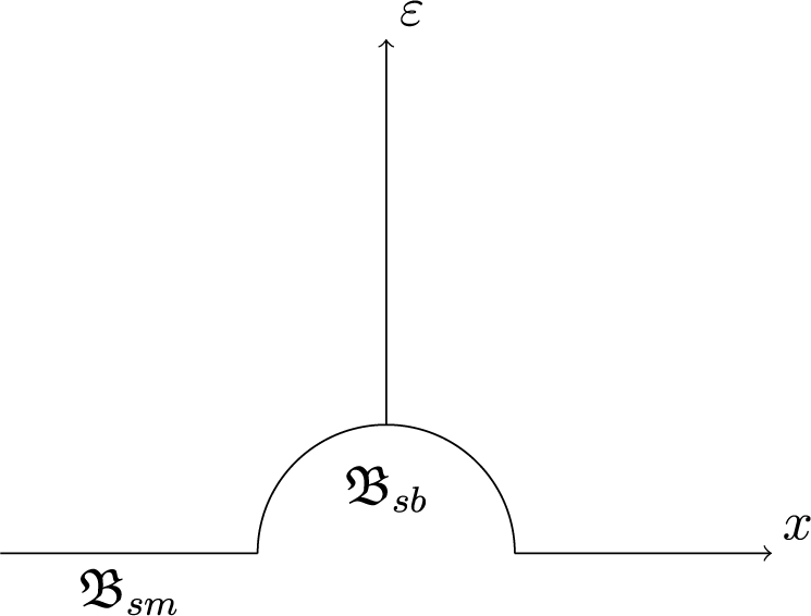


 Open access