

The use of 3D imaging within archaeology is surging in popularity because it expands, in astounding ways, the avenues used for addressing anthropological questions (Hirst et al. Reference Hirst, White and Smith2018; Remondino and Campana Reference Remondino and Campana2014; Weber and Bookstein Reference Weber and Bookstein2011). For example, researchers are able to reassemble fragmentary objects, reconstruct missing structures, mitigate taphonomic distortion (Benazzi et al. Reference Benazzi, Gruppioni, Strait and Hublin2014; Delpiano et al. Reference Delpiano, Peresani and Pastoors2017; Zollikofer et al. Reference Zollikofer, Ponce de León, Lieberman, Guy, Pilbeam, Likius, Mackaye, Vignaud and Brunet2005; Zvietcovich et al. Reference Zvietcovich, Navarro, Saldana, Castillo and Castaneda2016), advance geometric morphometric research (Baab et al. Reference Baab, McNulty and Rohlf2012, Reference Baab, McNulty and Harvati2013; Bastir et al. Reference Bastir, García-Martínez, Torres-Tamayo, Palancar, Fernández-Pérez, Riesco-López, Osborne-Márquez, Ávila and López Gallo2019; White et al. Reference White, Pope, Hillson and Soligo2022), improve upon the ways in which data are collected, and extract new types of data that cannot be collected directly from the object (O’Neill et al. Reference O’Neill, Angulo-Umana, Calder, Hessburg, Olver, Shakiban and Yezzi-Woodley2020; Schulz-Kornas et al. Reference Schulz-Kornas, Kaiser, Calandra, Winkler, Martin and v. Koenigswald2020; Yezzi-Woodley et al. Reference Yezzi-Woodley, Calder, Olver, Cody, Huffstutler, der Terwilliger, Anne Melton, Tappen, Coil and Tostevin2021, Reference Yezzi-Woodley, Terwilliger, Li, Chen, Tappen, Calder and Olver2024). And in the case of computed tomography (CT) it can be leveraged to nondestructively access otherwise inaccessible internal structures (e.g., the neurocranium, endocranium, or pneumatization and sinuses; Ponce de León and Zollikofer Reference Ponce de León and Zollikofer1999; Seidler et al. Reference Seidler, Falk, Stringer, Wilfing, Müller, zur Nedden, Weber, Reicheis and Arsuaga1997; Tobias Reference Tobias2001; Wu and Schepartz Reference Wu and Schepartz2009), virtually differentiate fossils from adhering matrix or infilled cavities (Bräuer et al. Reference Bräuer, Groden, Gröning, Kroll, Kupczik, Mbua, Pommert and Schiemann2004; Conroy and Vannier Reference Conroy and Vannier1984; Tobias Reference Tobias2001; Zollikofer et al. Reference Zollikofer, Ponce de León and Martin1998), or even view mummies inside their encasements (White et al. Reference White, Hirst and Smith2018; Wu and Schepartz Reference Wu and Schepartz2009). 3D models have been used for studies on biomechanics (O’Higgins et al. Reference O’Higgins, Cobb, Fitton, Gröning, Phillips, Liu and Fagan2011; Spoor et al. Reference Spoor, Wood and Zonneveld1994; Strait et al. Reference Strait, Weber, Neubauer, Chalk, Richmond, Lucas and Spencer2009; Weber et al. Reference Weber, Bookstein and Strait2011) and allometry and ontogeny (Massey Reference Massey2018; Penin et al. Reference Penin, Berge and Baylac2002; Ponce de León and Zollikofer Reference Ponce de León and Zollikofer2001). For objects where two-dimensional (2D) sketches are used widely, such as stone tools and pottery, 3D models have been used to create 2D technical drawings in a more time-efficient, consistent, and reliable manner (Barone et al. Reference Barone, Neri, Paoli and Razionale2018; Hörr Reference Hörr2009; Magnani Reference Magnani2014). 3D models have been used to refine typologies (Grosman et al. Reference Grosman, Smikt and Smilansky2008), and to analyze reduction and operational sequences (Clarkson Reference Clarkson2013; Clarkson et al. Reference Clarkson, Shipton and Weisler2014; Hermon et al. Reference Hermon, Polig, Driessen, Jans and Bretschneider2018). Zooarchaeologists and taphonomists are using 3D models generated via micro-computed tomography (micro-CT), micro-photogrammetry, structured light scanning, and high-power imaging microscopes to study bone surface modifications and surface texture (Arriaza et al. Reference Arriaza, Aramendi, Ángel Maté-González, Yravedra, Baquedano, González-Aguilera and Domínguez-Rodrigo2019; López-Cisneros et al. Reference López-Cisneros, Linares-Matás, Yravedra, Ángel Maté-González, Estaca-Gómez, Mora, Aramendi, Rodríguez Asensio, Barrera-Logares and González Aguilera2019; Martisius et al. Reference Martisius, McPherron, Schulz-Kornas, Soressi and Steele2020; Mate-Gonzalez et al. Reference Maté-González, González-Aguilera, Linares-Matás and Yravedra2019; Otárola-Castillo et al. Reference Otárola-Castillo, Torquato, Hawkins, James, Harris, Marean, McPherron and Thompson2018). These are but a few examples of the ways in which anthropologists are using 3D models in their research.
3D scanning has had major impacts on cultural heritage and data sharing. Digital models can be shared electronically, making them more accessible to researchers across the globe (Abel et al. Reference Abel, Parfitt, Ashton, Lewis, Scott and Stringer2011; Wrobel et al. Reference Wrobel, Biggs and Hair2019) through platforms such as MorphoSource, Virtual Anthropology, Sketchfab, Archaeology Data Service, Smithsonian3D, AfricanFossils.org, and tDAR (Bastir et al. Reference Bastir, García-Martínez, Torres-Tamayo, Palancar, Fernández-Pérez, Riesco-López, Osborne-Márquez, Ávila and López Gallo2019; Hassett Reference Hassett2018; Mulligan et al. Reference Mulligan, Boyer, Turner, Delson and Leonard2022; Wrobel et al. Reference Wrobel, Biggs and Hair2019). The ability to share digital models is especially pertinent for limiting research-related travel, thereby reducing its environmental impact, as well as maintaining continuity during disruptive events such as a pandemic. The ease with which models can be shared expands the possibilities for cultural heritage, education, science communication, and public engagement. Research-quality 3D models can be used to facilitate preservation by limiting the handling of the actual object (Means et al. Reference Means, McCuistion and Bowles2013; Pletinckx Reference Pletinckx2011). Furthermore, data collection from 3D models is inherently nondestructive (Wu and Schepartz Reference Wu and Schepartz2009). Not only are many repositories open-access resources, public institutions are increasingly creating virtual experiences that allow patrons anywhere in the world to explore archaeological sites and museums, such as those that can be found on the Archaeological Institute of America’s online education resource list. As a result of the push to create public-facing resources, publications have emerged describing methods for creating virtual exhibits and to explore ways in which 3D scanning can be used to engage the public (Abel et al. Reference Abel, Parfitt, Ashton, Lewis, Scott and Stringer2011; Bruno et al. Reference Bruno, Bruno, De Sensi, Luchi, Mancuso and Muzzupappa2010; Quattrini et al. Reference Quattrini, Pierdicca, Paolanti, Clini, Nespeca and Frontoni2020; Tucci et al. Reference Tucci, Cini and Nobile2011; Younan and Treadaway Reference Younan and Treadaway2015). Additionally, options are becoming available for educators to develop content that is more accessible through the application of 3D printing (Bastir et al. Reference Bastir, García-Martínez, Torres-Tamayo, Palancar, Fernández-Pérez, Riesco-López, Osborne-Márquez, Ávila and López Gallo2019; Evelyn-Wright et al. Reference Evelyn-Wright, Dickinson and Zakrzewski2020; Weber Reference Weber2014). As the field grows, journals (e.g., Digital Applications in Archaeology and Cultural Heritage, Virtual Archaeology Review, and the Journal of Computer Application in Archaeology), conferences, and professional organizations (e.g., Computer Applications and Quantitative Methods in Archaeology) are being established that are specifically devoted to the advancement of digital methods in archaeology. Finally, the rapid growth of the field has inspired conversations on the ethics of and best practices for engaging in digital methods within archaeology (Dennis Reference Dennis2020; Lewis Reference Lewis2019; Mulligan et al. Reference Mulligan, Boyer, Turner, Delson and Leonard2022; Richards-Rissetto and von Schwerin Reference Richards-Rissetto and von Schwerin2017; White et al. Reference White, Hirst and Smith2018), such as the FAIR (Findable, Accessible, Interoperable, and Reusable) guiding principles for scientific data management and stewardship (Wilkinson et al. Reference Wilkinson, Dumontier, Aalbersberg, Appleton, Axton, Baak and Blomberg2016) and the CARE (Collective benefit, Authority to control, Responsibility, and Ethics) Principles for Indigenous Data Governance established by the Global Indigenous Data Alliance. When scanning any objects related to material culture and human remains, as well as animal bone, it is important to identify key stakeholders and those who have data sovereignty to ensure appropriate permissions are acquired. Thus, we encourage the reader to explore the CARE principles before applying the methods we introduce here.
Photogrammetry, laser scanning, and structured light scanning are commonly used methods for creating 3D models of objects and are useful for creating high-resolution, textured scans (Lauria et al. Reference Lauria, Sineo and Ficarra2022; Linder Reference Linder2016; Magnani et al. Reference Magnani, Douglass, Schroder, Reeves and Braun2020; Niven et al. Reference Niven, Steele, Finke, Gernat and Hublin2009; Porter et al. Reference Porter, Roussel and Soressi2016a). Though Bretzke and Conard (Reference Bretzke and Conard2012) demonstrated how two objects can be scanned at a time, generally objects are scanned individually, and the scanning and post-processing times can be extensive. On the other hand, multiple objects can be scanned simultaneously using medical or micro-CT. The output Digital Imaging and Communications in Medicine (DICOM) files are then interactively surfaced before being separated into individual files and cleaned using expensive, proprietary and Graphical User Interface (GUI)-based software such as Slicer, Aviso, or Geomagic (Göldner et al. Reference Göldner, Karakostis and Falcucci2022). In these cases, the scanning process is efficient but at the cost of an increase in labor-intensive post-processing time and, like the other methods, may not be conducive to efficiently creating a full set of research-quality 3D models of objects from large collections.
The ability to feasibly scan large collections like faunal assemblages, which can be comprised of over 10,000 specimens, necessitates a significant decrease in the time required for processing and post-processing while retaining high-quality results useful for research. As such, scanning has been mostly restricted to small collections, or a small subset of a large collection, which imposes limitations on research requiring larger sample sets. The ability to expediently scan and model specimens from large collections opens possibilities for new types of data accumulation, which in turn provides access to methods such as machine learning and other powerful computational approaches designed to handle larger and richer datasets (Calder et al. Reference Calder, Coil, Melton, Olver, Tostevin and Yezzi-Woodley2022; Carleo et al. Reference Carleo, Cirac, Cranmer, Daudet, Schuld, Tishby, Vogt-Maranto and Zdeborová2019; Jordan and Mitchell Reference Jordan and Mitchell2015; McPherron et al. Reference McPherron, Archer, Otárola-Castillo, Torquato and Keevil2021; Yezzi-Woodley et al. Reference Yezzi-Woodley, Terwilliger, Li, Chen, Tappen, Calder and Olver2024; Zollikofer et al. Reference Zollikofer, Ponce de León and Martin1998). And, as stated previously, critical to the adoption of more efficient and cost-effective methods is ensuring that the output produces high-quality, research-ready models.
In this article, we describe a method that we have developed, which we call the Batch Artifact Scanning Protocol (BASP), to safely and rapidly scan large assemblages of objects using a medical CT scanner and to compare our results with published results using other scanning methods, particularly photogrammetry and structured light scanning, to illustrate the efficacy and efficiency of our method. While Göldner and colleagues (Reference Göldner, Karakostis and Falcucci2022) independently developed a similar packaging method for bladelets scanned via micro-CT, our method emphasizes automated post-processing workflows and is adaptable for different artifact types (e.g., lithics and pottery) and imaging modalities (i.e., micro-CT and CT).
For our research purposes we scanned experimentally broken ungulate limb bones. The DICOM data are automatically segmented and surfaced using an algorithm that can be executed in Python. Notably, a key contribution of this article is the automated post-processing and the detailed discussion of the factors to consider when weighing options for constructing 3D models useful for research. Thus, we begin by providing a straightforward step-by-step description of how to use BASP. Then we offer a detailed discussion of the difference factors influencing how to optimize use of the protocol, such that those who choose to use the protocol can take a nuanced approach, structured to provide the best outcomes for their project. The purpose of this article is to provide sufficient details in order to offer an inroad for those who are new to CT scanning, so that BASP can be adopted and built upon by independent research groups.
Materials
Our sample was comprised of 2,474 bone fragments drawn from a collection of experimentally broken ungulate appendicular long bones at the University of Minnesota that are being used in research on how early hominins used bone marrow as a food resource. We encased bone fragments in foam packets to facilitate the batch scanning process and to offer protection to the specimens during transport to the facility, as well as during scanning. The following materials were needed to create the scan packets: large rolls of polyethylene foam, a hot-glue gun, glue sticks, box cutters, and tape (we used painter’s tape). Packets were labeled using a Sharpie. The work was done on a large cutting mat to protect the surface of the work table. Large, military-grade duffel bags were used to transport scan packets to the facility where they were scanned. We also used a computer and camera (or smartphone) to document the fragment layout in a .csv file and to take photos as backup for documentation (see Figure 1).
Supplies needed for scanning: shown here are the supplies we used for scanning, which include polyethylene foam, a cutting mat, painter’s tape, a hot-glue gun with glue sticks, a utility knife, a smartphone for taking photographs for the purpose of documentation, and a laptop to create the .csv companion file. While this setup was chosen with the protection of the scanned objects in mind, it should be noted that any packaging material can be used, as long as its density is discernibly different from the target object during scanning.

Methods
Here we describe in detail the steps and procedures in the BASP, to produce high-resolution 3D surface models. This is broadly a three-stage process: (1) preparing specimens for scanning, (2) scanning, and (3) post-processing scans.
Prior to scanning we assembled the required materials and chose the specimens we wished to scan; next, bone fragments were placed in scan packets that were then transported to the scanning facility. Each specimen was carefully documented by specimen number in a .csv file for cross-referencing during post-processing. Fragments were scanned using medical CT. Subsequent DICOM data were processed using a Python algorithm that separated each fragment into individual files and segmented the fragment from the remainder of the image (what can be thought of as negative space), and then the segmented images were surfaced to create a 3D mesh. Surfacing is the process by which scan data are converted into a mesh that covers the surface of a solid object, which can then be used for computations and further processing. These meshes were then checked, and adjustments were made on individual fragments as needed. The time required for such manual interventions was minimized through the overall efficient and effective design of the scanning and segmentation protocols.
Preparing Specimens for Scanning
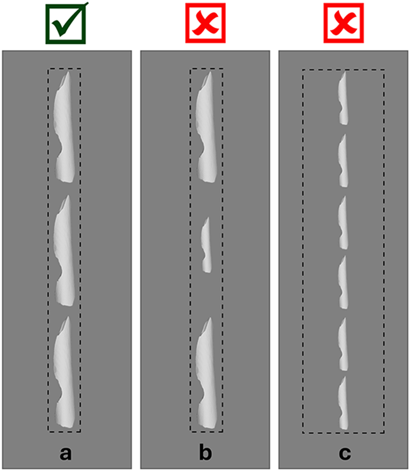
Bone fragments were packaged in polyethylene foam for transport and scanning. We cut out strips of polyethylene packaging foam and laid the bone fragments linearly, end to end, along the center of one of the foam strips to provide protection during transport and scanning. In order for the automated segmenting and surfacing algorithm to work properly, we allowed approximately 1–2 cm clearance between bone fragments in each packet. In order for the algorithm to successfully divide the scan into individual fragment files, there can be no overlap between specimens in the x- or y-directions (see Figure 2). The surfacing algorithm detects breaks between the fragments in the scan data and automatically separates the images according to those breaks. If there is overlap between two fragments, the algorithm may not recognize them as two fragments and may combine them into a single fragment or cut off parts of one or both fragments. We also ensured a 3–5 cm margin along the edges of the packaging material to accommodate the glue used to seal the packets closed.
Fragment placement: the fragments should not overlap in the x- or y-directions. This ensures that the automated segmentation can properly separate the fragments within the scan data into individual models for surfacing. The x-axis is the view from the side of the scanning bed. The y-axis is the bird’s-eye view of the scanning bed.

For each packet, we chose fragments that are similar in size in the x- and y-directions in order to conserve material, because several strips of foam were used for each packet. We stacked the foam strips one on top of the other until the stack was high enough to comfortably cover the utmost top edge of the fragment, thus providing protection for the specimen in all directions.
Documenting Specimens
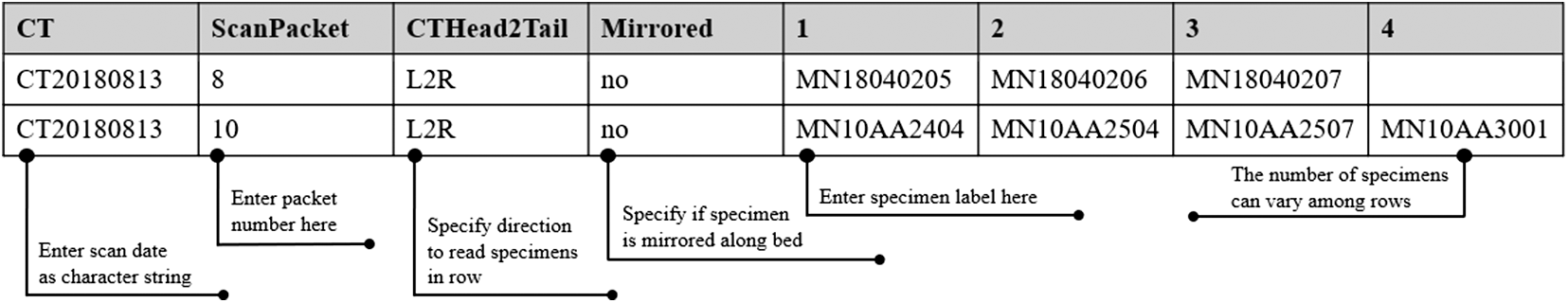
Documenting the layout of specimens is a key component of the preparation process and, ultimately, post-processing. Once the bone fragments were arranged in the desired order along the first packaging strip, the specimen catalog number was recorded in a .csv file (see Figure 3). (A template can be downloaded from the AMAAZE website and GitHub.) It is essential to adhere to the prescribed .csv file format for the algorithm to function properly. It is equally important to label the “head” of the packet such that it is placed properly on the CT scanning bed. Each line item in the .csv file is dedicated to one packet, and the algorithm reads the line from left to right (preferably “head” to “foot” on the scanning bed). Therefore the leftmost entry in the .csv file is generally at the “head” of the packet. Should there be an error when the packet is placed on the bed, such that it is scanned from “foot” to “head,” then the entry for the column labeled “CTHead2Tail” can be changed to “R2L,” so that the line is read in the opposite direction. This happened a couple of times owing to user error, and our method can easily handle it in post-processing.
Documenting specimens for scanning: here we provide an example of how to complete the formatted .csv so that the segmentation and surfacing algorithms will function properly. The first column indicates the date (YYYYMMDD), the second column indicates the packet number for that date, the third column indicates the direction the code should read the .csv file, the fourth column indicates whether or not the scan was mirrored, and the remaining columns indicate the specimen labels. The third and fourth columns are there to mitigate the need to resurface the scan should it have been oriented improperly on the scanning bed.

Figure 3 Long description
The table has eight columns: CT, ScanPacket, CTHead2Tail, Mirrored, Column 1, Column 2, Column 3, Column 4. Row 1: CT CT20180813, ScanPacket 8, CTHead2Tail L2R, Mirrored no, Column 1 MN18040205, Column 2 MN18040206, Column 3 MN18040207, Column 4 blank. Row 2: CT CT20180813, ScanPacket 10, CTHead2Tail L2R, Mirrored no, Column 1 MN10AA2404, Column 2 MN10AA2504, Column 3 MN10AA2507, Column 4 MN10AA3001.
We took photographs of how the fragments were laid out on the foam strip for reference and backup, in case there were errors when recording information in the .csv file. A wide-angled shot of the entire layout of the package was taken, with the package number displayed in the front and center of the image (see Figure 4a). Pictures of the layout of each fragment were taken as well. The specimen number for the individual bone fragment was clearly visible in the image, along with a part of the previous bone specimen for context (see Figure 4b). Some fragments were not directly labeled, but rather stored in individual bags that bore the specimen label. In these instances, the bag was placed above the fragment for the picture (see Figure 4c). Once the packages were sealed, the bags were taped to the outside of the scanning package for ease of repackaging later.
Fragment layout: here we offer images of the various stages of the packaging process. (a) We took a photograph of the layout of the fragments for the entire package. (b) Photographs were taken of individual fragments such that we could clearly see the labels. (c) If the fragment was not directly labeled, we included the labeled bag in the photograph. (d) We traced the fragments using a Sharpie and then used the outline to cut out sections in the foam to encase the fragments (f). Packets were wrapped in tape for additional protection during transport (e).

Packaging Specimens for Transport and Scanning
Once the layout was established and recorded, we carefully used a Sharpie to trace the fragments, being mindful not to get ink on the fragments (see Figure 4d). The outlines were later used as guides for cutting cavities in the foam that add additional protection to the specimens. The outlines can be slightly larger than the fragment itself. A thin-tipped Sharpie can be used for smaller fragments in order to produce a more accurate outline. After outlining, the specimens were removed from the strip and set aside. All but two of the remaining foam strips were glued to the back of the outlined strip using a hot-glue gun. This ensures that the strips will form one cohesive stack (see Figure 4f). Once the glue set, we followed the outlines, using box cutters to cut holes in the stack of glued foam. The foam that was removed was set aside in the order that it was cut out so that it could be used later in the process to add padding if additional protection was needed (see Figure 4e).
After the foam had been cut to create cavities for each bone fragment, the styrofoam stack was flipped upside down to properly attach the bottom piece of the structure. One of the single strips of styrofoam previously set aside was used for the bottom piece. When specimens were heavier, we added additional layers to the bottom and top to prevent the bone fragments from falling out of the packaging during transport and scanning. In some cases, especially when packaging smaller fragments, we cut out the cavities prior to gluing, so that we could apply glue near to the edges that were cut to ensure that fragments would not escape the cavity and slip in between the layers of foam.
Having securely glued the base to the bottom of the package, the stack was flipped right-side up and the first specimen cavity (i.e., the “head”) was placed to the left side, to remain consistent with the format in the .csv file. We placed individual bone fragments into their corresponding cavities in the same orientation in which they were outlined. Care was taken to place the specimens so they were not likely to move around in transit. As needed, the excess pieces of foam taken from the outline cuttings were used to fill in any gaps between the edge of the cavity and each fragment. This was to prevent unintentional damage related to movement in the cavity and to ensure alignment of the fragments along the z-axis.
Once we were satisfied with the placement of the bones inside the package and their relative inability to move around in transit, the final foam strip was secured to the top of the package. Care was taken not to get glue on the fragments. After constructing the packet, we wrapped a strip of painter’s tape around the entire shorter circumference at the head of the packet and then labeled the tape with the packet number (see Figure 5) and the word “Head,” so that the CT technicians we worked with knew how to place the packet on the scanning bed and what number to use in the filenames for the output data. Additional strips were added to any section of the packet where extra protection seemed necessary, such as in between two larger fragments or in the middle of long fragments that were at risk of breaking. The completed packets were then ready to go to the scanning facility (see Figure 6).
Pictured here is an example of how we labeled the package, indicating how to orient the package on the scanning bed, and as a cross-reference for the .csv file for that scan package.

Prepared packets were designed for rapid placement onto the scanning bed, minimizing handling time and maximizing efficiency. This approach significantly reduced scanning time and costs, especially in facilities that charge by the hour.

Scanning
We brought a total of 2,474 bone fragments in 329 packets to the Center for Magnetic Resonance Research at the University of Minnesota. Each packet was scanned individually. Each scan takes a couple minutes, including the time it takes to lay the packet on the scan bed, adjust the field of view, and take the scan. Once all scans were completed, the data were exported as DICOM files.
A Siemens Biograph 64-slice Positron Emission Tomography (PET)/CT was used to scan the packets. The scanning parameters are provided in Table 1. We provide a high-level description of these parameters in Supplementary Material 1. For more detailed, technical descriptions of how CT scanning works, see Buzug (Reference Buzug, Kramme, Hoffmann and Pozos2011), Scherf (Reference Scherf2013), Sera (Reference Sera, Soga, Umezawa and Okubo2020), Spoor and colleagues (Reference Spoor, Jeffery and Zonneveld2000), and Withers and colleagues (Reference Withers, Bouman, Carmignato, Cnudde, Grimaldi, Hagen, Maire, Manley, Plessis and Stock2021). Using medical CT scanning will likely require working with a trained radiologist, who can determine the appropriate settings for achieving an optimal image. Thus, a basic understanding of these parameters can be useful for discussing the needs that are particular to the project, with the radiologist, for example, capturing trabecular bone, working with fossilized material, and navigating matrix in-fill or adhesion, all of which can be effectively mitigated using CT.
CT Parameter Settings.

Table 1 Long description
The table lists computed tomography acquisition and reconstruction parameter settings. Spatial sampling is set to 0.6 mm slice thickness with a matching 0.6 mm reconstruction interval. Exposure settings are 80 kV tube voltage and 28 mA tube current. The gantry rotation time is 0.05 seconds and the pitch is 0.8. Image reconstruction uses a bone window algorithm with a B60f sharp convolution kernel. These values describe the protocol configuration and do not by themselves indicate image quality or patient dose without additional scanner and patient details.
Note: Please see Supplementary Material 1 for more details on these parameters.
Post-processing
Detailed written instructions for creating the 3D models from the DICOM scan data can be found on the AMAAZE GitHub, along with the AMAAZEtools package required to run the CT-Surfacing scripts in Python. Installation instructions accompany the packages on the AMAAZE GitHub. We have also provided data from two scans (scans 8 and 10), each containing four fragments, and an accompanying .csv file, so users can try the process without having their own DICOM data. In summary, to begin the process of surfacing the scans to create the models, the AMAAZEtools packages must be installed, and one must have the appropriate DICOM files and the properly formatted .csv file.
The first step is to separate the multifragment files into single-fragment files. This is done by running the Python script called dicom_firstpass.py, which automatically segments the file into individual fragments and outputs images of the segmentation with bounding boxes (see Figures 7a and 7b), as well as the bounding box coordinates, as a .csv file that can be manually edited as needed.
Automated segmentation: here we provide examples of the .jpg images output by the automated segmentation algorithm, which illustrates how the algorithm separates individual fragments from the scan data. These examples come from a session during which we scanned multiple packets. These scans come from packets 8 and 10 in that series. Note: These are the scans that are provided, along with the source code, offering researchers the opportunity to practice this protocol prior to acquiring their own scan data.

The algorithm for automatically separating multiple bone fragments from a single CT scan works by first thresholding the CT image at a user-specified value in Hounsfield units (HU). The specific threshold depends on the material under consideration; for bone fragments, we use 2,000 HU. The thresholded binary images are then projected onto each 2D view of the length of the scanning bed, and the bone bounding boxes are identified by taking the largest connected components of the projected binary images and adding padding on each side. See Figures 7a and 7b for a depiction of the computed bounding boxes for each bone for the test scan provided in GitHub.
The automatic algorithm works very well, but there can be occasions when the automatically detected bounding boxes are incorrect. The user can determine this by examining the scan overview images (see Figures 7a and 7b), which depict the bounding boxes over a 2D projection of the scanning bed. In this case, adjustments can be made by editing the ChopLocations.csv file that was automatically generated by dicom_firstpass.py prior to the next step in the processing. The ChopLocations.csv file contains the (x, y) pixels’ coordinates, indicating where the bounding boxes start and stop. The file is initially generated by the automatic algorithm but can be easily adjusted by the user as needed. After modifying the ChopLocations.csv file, the script dicom_refine.py will generate new bounding boxes based on the modified data in the chop locations file, which will also generate new scan overview images, which the user can view to see if the bounding boxes are correct. This process can be iterated several times, if necessary, until the bounding boxes are correctly specified. Again, let us emphasize that the failure cases in the method are very rare, and, for the vast majority of the scans, no refinements are needed, although our method makes it easy to refine the bounding boxes when necessary.
Once the files are segmented properly, the next step is to run surface.py to generate triangulated surface 3D models for each object in the CT scan. (See Figures 8a and 8b for examples of completed models.) The surfaces are generated from the CT images with the Marching Cubes algorithm (see Lorensen and Cline Reference Lorensen and Cline1987). The user must provide a threshold parameter (called iso in the code) for the surfacing. As in the segmentation part above, the iso threshold value is material-dependent and may also depend on the size of the objects, amount of fine detail, and the resolution of the CT scanner. For surfacing bone fragments we normally use iso = 2500, with some manual adjustments in special cases. The surfacing script reads the CT resolutions, which are often different between slices, compared to within each 2D slice, from the DICOM header files and scales the resulting mesh so that the units are millimeters in all coordinate directions. Choosing good thresholds is largely application-dependent. Larger threshold values may omit fine-scale details, while small threshold values will pick up on noise and scanning artifacts. When scanning bone fragments, lower values are useful when the bone is extremely thin or more porous, and lower values capture trabecular bone better than higher values. The surface.py script also has the capability to generate rotating animations (as .gif files) of each object that has been surfaced. All the meshes are output as individual .ply files.
Pictured here are the final meshes from the previous figure of scans 8 and 10.

Results
Here we compare the BASP presented here with other scanning methods and compare our results with scanning and post-processing times that have been published by independent research teams. We attempted other approaches to scanning before deciding to develop the BASP and share our experience exploring these options, as well as data extracted from the literature. Advancements in all these scanning approaches are ongoing, and thus the published literature likely does not reflect the substantial increases in speed of scanning and post-processing that have been achieved to date. Nonetheless, the protocol we present here is a tremendous advancement in this regard.
For our purposes, photogrammetry proved to be ineffective, owing to issues of translucency and reflectivity. However, we scanned fragments using the David structured light scanner and David software on a high-end desktop (Dell computer with Microsoft Windows 10 Enterprise OS, 2.7 Quad-Core Intel Core i7, 128 GB RAM). Images were captured every 15°, with a total of 24 captures per 360° rotation. We found that it takes approximately 5–10 minutes to set up the specimen. Scanning takes between 15 and 25 minutes. Typically, it takes at least two rounds of scanning to capture the entire fragment, because the fragment needs to be flipped after the first round to capture the portion that was mounted and inaccessible to the scanner in the first round. Once scanning is complete, post-processing is required. For this, we used the David software in conjunction with Geomagic Design X, which is a computer-aided design (CAD) software package. The time it takes to post-process can vary considerably, based on the degree to which the scans need to be cleaned and the number of challenges that arise during alignment and registration (see Bernardini and Rushmeier Reference Bernardini and Rushmeier2002). Based on our experience, it takes on average between 15 and 60 minutes to post-process the scans to create the 3D model. To set up, scan, and post-process 2,474 fragments to make 3D models would minimally take 3,505 hours of interactive user time, or 85 minutes per fragment.
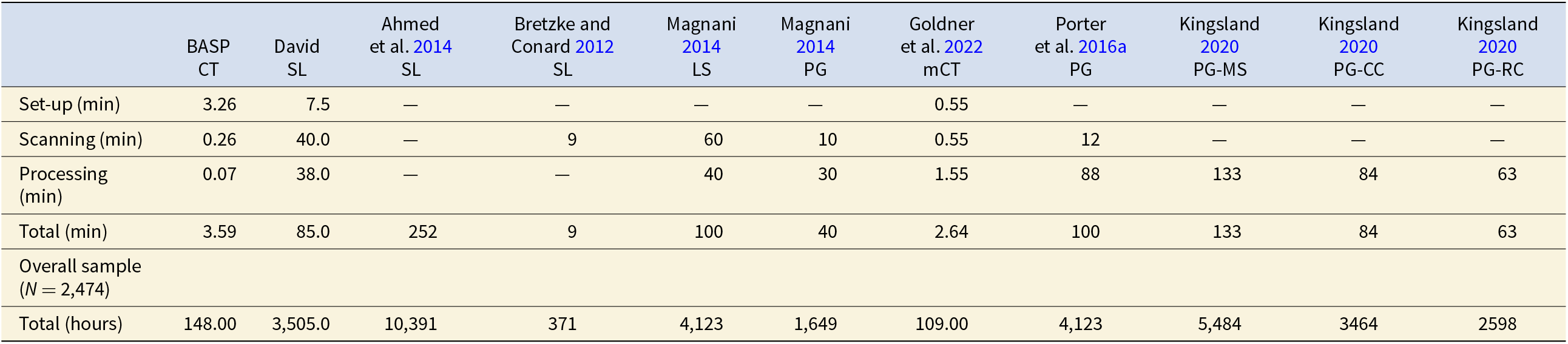
On the other hand, with the CT scanning method described here, each packet takes between 15 and 30 minutes to assemble. We ended up with a total of 329 packets, and, on average, there were 7.5 fragments per packet. Overall scanning time was 10.75 hours. The post-processing is very fast: it takes 35 seconds to surface all eight bone fragments in the example GitHub repository using a standard laptop computer, amounting to about 4.375 seconds per fragment. To surface the whole collection takes slightly under three hours. This means that to create a single 3D model of a bone fragment using the structured light scanner took 85 minutes, whereas it only took three minutes using medical CT (see Table 2).
Comparison of Scanning and Processing Times Per Specimen.

Table 2 Long description
The table compares per-specimen time in minutes for set-up, scanning, processing, and total time across multiple 3D capture methods, plus the projected total hours to complete a sample of 2,474 specimens. BASP CT has the lowest total time per specimen at 3.59 minutes, made up of 3.26 minutes set-up, 0.26 minutes scanning, and 0.07 minutes processing, totaling about 148 hours for the full sample. Goldner et al. 2022 micro CT is also relatively fast at 2.64 minutes per specimen and about 109 hours overall, with short set-up and scanning but higher processing than BASP CT. David structured light totals 85 minutes per specimen and about 3,505 hours overall, driven by long scanning and processing times. Photogrammetry examples are generally much slower overall: Magnani 2014 photogrammetry totals 40 minutes per specimen and about 1,649 hours, Porter et al. 2016a totals 100 minutes and about 4,123 hours, and Kingsland 2020 ranges from 63 to 133 minutes per specimen depending on software, corresponding to about 2,598 to 5,484 hours. Some studies have missing set-up, scanning, or processing values shown as dashes, so their reported totals may understate true time costs and comparisons should be interpreted cautiously.
Notes: We reviewed several examples from the literature since 2012 to assess the relative efficiency of our method. In this table, we calculated overall time based on our sample size (N = 2,474). For studies reporting time ranges, we recorded the average value. These examples represent published papers detailing scanning and post-processing times. Some of the data from all comparative samples, such as set-up time and post-processing times, are either missing or partially reported; thus, the overall time costs for these methods are greater than what is reported here. Cells with missing or partially reported data contain em-dashes. While we acknowledge, through personal communications and our ongoing work within the realm of 3D modeling, that scanning equipment and techniques are becoming increasingly faster, this progress is not yet fully reflected in the literature. To our knowledge, the protocol we present here remains unmatched by these advancements. Abbreviations: BASP=Batch Artifact Scanning Protocol, CT=medical CT, mCT=micro-CT, SL=structured light, LS=Laser Scanner, PG=photogrammetry, MS=MetaShape, CC=ContextCapture, RC=RealityCapture. “Set-up” refers to the time, in minutes, to set-up an individual specimen for scanning. “Scanning” refers to the time, in minutes, to scan an individual specimen. “Processing” refers to the time, in minutes to process the scan data to achieve 3D models. “Total” refers to the time, in minutes to model a single specimen. “Overall” refers to the overall time it would take in hours to scan our sample N=2,474.
We compared our time costs to several other examples in recent literature. Unfortunately, in all cases, details of the time costs are missing, and thus the overall time expense found in the literature is lower than the actual overall time taken to create the 3D models. Nonetheless, it is a useful tool for general comparison. Ahmed and colleagues (Reference Ahmed, Carter and Ferris2014) explored the effectiveness and efficiency of an assembly-line approach to 3D scanning of artifacts with the help of nine 3D specialists, one of whom scanned and the remaining processed scans. They scanned a total of 300 artifacts comprised of a variety of materials and found the process took roughly 1,260 hours. They used four structured light scanners, each set up for different-sized objects. Captures were taken every 30° (12 scans), and then flipped and scanned again to capture the other side. Generally 48 scans were required for a complete model, and it took about 20 minutes to capture the 48 scans. The macro-scanner and the larger objects (Scanner A) generally took more scans, sometimes up to 96 scans. Since they did not offer a complete breakdown of time costs, we divided the total pre- and post-processing time (1,260 hours) by the number of artifacts (N = 300). Thus, to scan and create a 3D model of one object took 4.2 hours. To scan our sample would take 10,391 hours. It should be noted that this post-processing also involved creating digital museum environments for the display of the 3D models; thus, in this case, the times are likely inflated.
Bretzke and Conard (Reference Bretzke and Conard2012) presented a method to assess variability in the morphology of lithic artifacts (cores and blades) using 3D models, thus demonstrating the potential for using 3D models for lithic analysis. They used SmartSCAN by Breukmann to scan and then OptoCad software to turn point clouds into meshes. They scanned cores one at a time and blades two at a time. They said they could scan five cores or 10 blades in approximately one hour. Their post-processing and set-up times were unspecified, so their overall time costs are likely underestimated. That said, a sample might generally have more blades than cores, which would offset the additional time costs not reported. With the available information, it takes nine minutes to create a 3D model of an individual object and would take 371 hours to scan a collection of 2,474 fragments.
Magnani (Reference Magnani2014) sought to demonstrate the capabilities of laser scanning, and potentially photogrammetry, as methods for replacing hand-drawn lithic illustrations. They scanned various lithic artifacts (Mousterian-type scrapers and denticulates, two cores, and one Achulean handaxe). They used a NextEngine desktop laser scanner with ScanStudio software, and they also used photogrammetry with a Canon DSLR and Agisoft software. Using the NextEngine, they took nine captures (every 40°) per 360° rotation. They scanned the object, flipped it upside down, and scanned it again. Each orientation took 30 minutes to scan, thus 60 minutes per object. Post-processing took approximately 40 minutes per object. When using photogrammetry, they took about 30 photos per object, and it took 10 minutes to photograph each object. The object was stationary, and the camera moved around it. Post-processing for a mid-range quality object in Agisoft took 30 minutes per object. They said that high-quality models could sometimes take several hours per object, so they chose the mid-range quality. They did not report set-up times in either case; however, we imagine it would be similar to the times we report here when using the David scanner. Regardless, even without the set-up times, according to these data, laser scanning would take 100 minutes per object and 4,123 hours to scan 2,474 objects, and photogrammetry would take 40 minutes and 1,649 hours respectively.
Göldner and colleagues (Reference Göldner, Karakostis and Falcucci2022) independently developed a batch scanning process they refer to as the StyroStone method. This is the closest to our method, as the preparation for scanning is quite similar; however, the post-processing is done manually via GUI, and they scanned bladelets using micro-CT, whereas our method focused on medical CT and utilizes an automated post-processing protocol. They post-processed the bladelets in Aviso and Artec Studio software packages. The authors acknowledge this, stating, “Although the scanning procedure could be accomplished over a short period of time, the subsequent extraction was time-consuming” (Göldner et al. Reference Göldner, Karakostis and Falcucci2022:4). Each of their packets could contain up to 220 bladelets. Their post-processing comprised of the following parts: (1) make the packets, (2) scan, (3) model extraction, (4) cropping extracted surfaces, (5) additional cropping, and (6) final cropping. Part 1 takes two hours, Part 2 takes two hours, and Part 3 takes two hours for the packet plus an additional minute per item, so, in the case of their largest packet, 340 minutes. It is not clear how long the remaining multistep parts (parts 4–6) take. Given that this is a GUI approach, it is entirely possible that these parts could take a considerable amount of time. In fact, their time costs (without parts 4–6) are 2.64 minutes per specimen, which would be approximately 109 hours for 2,474 specimens, whereas the method we share here takes 3.53 minutes per specimen and 146 hours overall. The time difference per specimen is 53.4 seconds. Given that parts 4–6 involve a GUI-based approach, it is not feasible to complete them in that time frame.
Furthermore, a direct comparison is complicated by the fact that they used micro-CT, which has considerably longer scanning times, whereas we used medical CT. As a result, their overall setup and scanning took considerably longer than our scanning time; however, each of their scans contained up to 220 objects, whereas ours only contained seven objects on average (see Supplementary Material 1 for a list of packets and the number of specimens in each packet). We could scale up the number of objects per packet, thus reducing the per specimen scanning time, and our post-processing times would remain exponentially faster. Furthermore, our post-processing method is automated and does not require constant user interface and oversight. If our method were to be scaled up to packages with 220 fragments, we would expect the overall time to be approximately 26 hours for a sample of 2,474.
Porter and colleagues (Reference Porter, Huber, Hoyer and Floss2016b) designed a low-cost portable photogrammetry rig. It took them 12 minutes to photograph both sides of an object. They did not track their post-processing times for this sample, and they acknowledge that these times can vary tremendously. However, they did report post-processing times for another ongoing study where they found it took between 43 minutes and 2 hours and 13 minutes (133 minutes), depending on the desired quality of the model (medium or high). Note that some of the post-processing time is automated.
Kingsland (Reference Kingsland2020) focused solely on comparing three different post-processing softwares used in photogrammetry: Agisoft Metashape, Bentley ContextCapture, and RealityCapture. They scanned an aryballos (small, globular flask, 4 cm wide, 18 cm tall) from the Farid Karam Collection. The object was oriented twice (upright and upside down), and 24 images were captured for each of three angles (high angle, middle angle, low angle) per orientation. They calculated average post-processing times and found that Metashape required 133 minutes per object, whereas ContextCapture took 84 minutes, and RealityCapture necessitated 63 minutes.
Discussion
Choosing an appropriate scanning method for research requires, at minimum, a consideration of the following: (1) portability, if required; (2) cost; (3) time; (4) computational resources, including memory, speed, graphics processing units (GPU), and storage; (5) whether or not texture is needed; (6) required scan resolution; and (7) the geometry that needs to be captured.
The location of the collection that needs to be scanned is the first concern. If the collection cannot be transported to a scanning facility, then the scanning equipment must be transported to the collection, which eliminates the opportunity for CT scanning. In these cases, the time to scan can increase considerably, especially when working with large collections.
Primary considerations when engaging in 3D scanning are how much time and how much money it will take. Methods like photogrammetry are extremely cost effective (Porter et al. Reference Porter, Roussel and Soressi2016a). Photogrammetry, laser scanners, and structured light scanners are portable and can be taken into the field. However, they are limited to scanning a single object at a time; moreover, it takes a considerable amount of time per scan as compared with the method presented here. Although this is not so problematic when the sample size is small, zooarchaeological assemblages can contain more than 10,000 specimens, thus making the use of portable scanners untenable. The method presented here thus fills a niche where large quantities of research-quality models need to be created from specimens that can be transported to a CT scanning facility.
Very few medical CT and micro-CT scanners are portable, and it was too cost-prohibitive to purchase the equipment (≥100,000 USD) ourselves. Therefore, to use BASP, we made arrangements to transport specimens to medical scanning facilities and paid fees for scanning services. In total, 329 packets were required to transport and scan 2,474 bone fragments. Some facilities will charge per scan, while others will charge an hourly rate, and rates can vary considerably among institutions and departments. By choosing an hourly rate we were able to scan 2,474 specimens in 93.75 hours for 2,900 USD.
Selecting Specimens to Scan
When choosing specimens for scanning, one of the most important factors to consider is scan resolution. Choice of the appropriate scan resolution will depend on the research question, the size of the object that needs to be scanned, the capabilities of the scanner, and the field of view used during scanning. Though it may seem counterintuitive, the highest possible resolution is not always the best option. Optimal resolution depends on the scale required to address the question. Though high resolution scans can serve as a reference, and can always be automatically decimated (i.e., the number of polygons in the surface mesh can be reduced) as required in order to streamline computational algorithms, they can radically increase computer processing times at all stages of the project, including the initial scanning, which may be prohibitive when working with large samples, especially when the size of the files impacts the ability of the computer to store them in memory.
Running test scans is recommended to verify the minimum size required for achieving usable models. For our research purposes, we needed to capture the macromorphology of the bone fragment in order to extract global features and measure angles along the fractured edges of the fragment. We chose to scan fragments that are ≥2 cm in maximum dimension, but we found that fragments ≥5 cm offer more visually appealing models. It is crucial to distinguish between visual appeal and data robustness. A model that looks visually impressive may not be necessary for research purposes, especially if the required data or measurements are more global; that is, we want to avoid confusing aesthetic detail with research readiness, and to assess needs based on the types of data that are to be collected or the purpose of the 3D model (e.g., museum displays vs. research). Other considerations include how thin the bone is (i.e., areas of translucence) and the relative dimensions of the fragment.
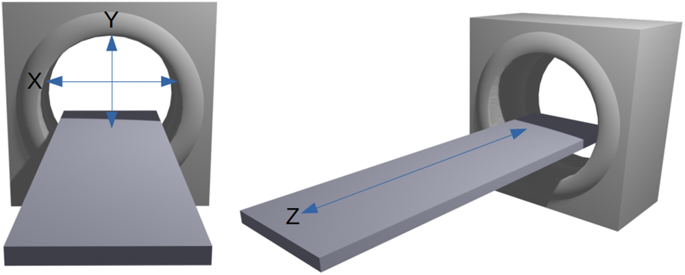
Figure 9 illustrates the standard directional axes conventionally used in medical CT scanning to orient the subject of scanning on the bed. The x-axis extends across the width of the bed. The y-axis extends from ceiling to floor, and the z-axis runs along the length of the bed. The bed moves along the z-axis. An object that is oriented such that its longest dimension aligns along the z-axis will result in a better scan than an object with its shortest dimension aligned along the z-axis. This is an important consideration for scanning objects such as long bone fragments that tend to be longer than they are wide.
Directional axes used in CT scanning.

Additional Considerations When CT Scanning
The Hounsfield unit (HU) is a key concept of CT scanning that refers to radiographic density (Scherf Reference Scherf2013). Materials are associated with specific HU. Water sets the starting point, at 0 HU. Materials with lower radiodensity, such as fat, have a negative HU (–120 to –90). Cancellous bone ranges from 300 to 400 HU, and cortical bone ranges from 500 to 1,900 HU; therefore, it is necessary to consider variation in the composition of the object to be scanned. This is especially important when CT imaging osteological materials and fossils coming from archaeological contexts. Bones that have fossilized may require different HU values from fresh bone (Spoor et al. Reference Spoor, Jeffery and Zonneveld2000). Additionally, if adhering matrix has an HU similar to that of the fossil, then it will be difficult to distinguish using CT. Conversely, in situations where the HU values are different, CT can be a way to “remove” adhering matrix without damaging the fossil (Conroy and Vannier Reference Conroy and Vannier1984; Zollikofer et al. Reference Zollikofer, Ponce de León and Martin1998). In fact, this is something to bear in mind when choosing the materials for creating scan packets: one needs to ensure that the HU differs from that of the target object, whether it be adhering matrix or packaging material. Many material types can be captured using CT, and it is not limited to bones or fossils. As an example, Göldner and colleagues (Reference Göldner, Karakostis and Falcucci2022) established that micro-CT—and thus medical CT—can be used to scan stone tools, and Kaick and Delorme (Reference van Kaick and Delorme2005) offer an overview of objects scanned in archaeology (e.g., sarcophagi and bronze statues), soil science, the timber industry, industrial inspection, and aviation security. The key to applying our methods is to ensure that the packaging material can be separated based on a threshold value, that is, the packaging material must be of a distinguishably different density from that of the object being scanned.
An important parameter for the CT scanner is the field of view (Miyata et al. Reference Miyata, Yanagawa, Hata, Honda, Yoshida, Kikuchi, Tsubamoto, Tsukagoshi, Uranishi and Tomiyama2020). As the package size in which the fragments are placed increases, the field of view required by the scanner increases along with it. If this is due to an increase in the number of fragments in the packet, then the disparity in the size of each individual fragment and the overall field of view causes the quality of the scan to decrease. This is less of an issue if it is related to an increase in fragment size. By narrowing the field of view so that the scan is tightly focused around the line of bone fragments on the scanning bed, we can obtain higher-resolution images compared with using a field of view that encompasses the whole width of the bed (see Figure 10). For this reason, we chose to create scan packets with similarly sized fragments, and because the fragments were generally small, we chose to limit the number of fragments in each packet. Our CT scans have a resolution of 0.6 mm between slices (along the direction of the scanning bed), and approximately 0.15 mm resolution within slices with a narrow field of view. It is possible that with a much higher-resolution CT scanner, multiple packets could be scanned in parallel while maintaining sufficient resolution, which would substantially decrease overall time costs.
Field of view: for the best resolution, the boundaries of the field of view should be as close to the target objects as possible (a). If specimens are disparate in size, the resolution of the smaller specimens will diminish (b). If the field of view is wide, this will also compromise resolution (c).

Computational expenses are another important consideration and are largely centered on memory and processing power (e.g., memory, storage, GPU, and speed). We have found that DICOM files require approximately 100 MB of storage space per bone fragment, but of course this depends on resolution. Thus, the collection described in this article takes roughly 250 GB of storage space for the DICOM files on disk. After surfacing to create 3D triangulated surfaces for each object, the resulting meshes take, on average, 10 MB per fragment. For our purposes, we purchased two 2 TB external drives to transport files from the scanning facility so that we could surface them on our computers. The BASP does not require any visualization software packages as part of the post-processing, which generally requires some form of GPU. For example, Geomagic requires a GPU with a minimum of 2 GB of memory, and in some cases 4 GB, and Aviso requires a GPU with a minimum of 1 GB. Running the surfacing step of BASP involves purely central processing unit (CPU) computations, and hence the post-processing can be performed on any computer without a GPU. On a high-end laptop computer (MacBook Pro, 2 GHz Quad-Core Intel Core i5, 32 GB RAM) we were able to process each bone fragment in 4.375 seconds. Of course, faster computers and parallel processing can be used to accelerate the process, as needed.
Beyond the logistics of scanning, it is necessary to consider what types of data need to be collected from the object. In particular, one must decide whether texture is required, determine the level of resolution required to answer the research question, and choose the parts of the object that need to be captured; for example, whether or not this includes internal structures (Bernardini and Rushmeier Reference Bernardini and Rushmeier2002). In the simplest description, image texture refers to the perceived textures that are visible when looking at the object in real life (see Figure 11) and in image processing are defined by a series of texture units that describe a pixel (vertex or voxel) and its neighborhood (He and Wang Reference He and Wang1991). Because our research focuses on the analysis of shape, we had no need to capture texture, making CT a viable option. The laser scanners and structured light scanners can often capture texture; however, this will increase processing times. The estimates provided in Table 2 are based on fragments that were, in both cases, scanned without capturing texture.
Texture: this a 3D mesh of a rock cairn at Gooseberry Falls. The image on the left is without texture. The image on the right has texture (scanning and 3D model created by Samantha Thi Porter).

Resolution can be thought of as the level of detail present in the model: higher resolution offers more detail. A mesh is comprised of a certain number of points, often referred to as vertices, and the interpolated information in between those points. More points within a given area increase the detail of the model. That said, higher resolution is not always necessary and adds time to computational processes when working with the model. If one were to model a flat plane, only three points would be necessary to uniquely specify it. However, as the object increases in complexity, more points are needed to capture that complexity. The resolution of the scanner is the limiting factor determining what can be expected for the resolution of the final 3D model. In our case, the CT scanner offered a resolution of 0.6 mm between slices and approximately 0.15 mm within slices (see Supplementary Material 1 for more details).
Because we needed more global features that did not require minute detail, a medical CT was sufficient. If a higher resolution is required, then the post-processing methods presented could be applied to micro-CT scan data. We have code that can be applied to .DICOM and .tiff files. Though file types may change the applicability of our protocol, it would only require a very small change to the code to make this adjustment.
An equally important consideration pertaining to resolution is scale. One can imagine zooming in on an image of the eastern coastline of Florida, as in Mandelbrot (Reference Mandelbrot1975). As one zooms in, the general outline between land and water will appear, then more curves along the shoreline will become visible, and ultimately one would be able to see the outline of individual grains of sand. If all that is needed is the general outline, then it would be computationally expensive to capture detail enough to see the grains of sand. Therefore, it is wise to consider the scale at which the research is being conducted and the required level of detail. That said, BASP can be effectively applied to images captured using a micro-CT with a flat scanning bed. Moreover, recent developments, outlined in O’Neill and colleagues (Reference O’Neill, Yezzi-Woodley, Calder and Olver2024), show how we are currently expanding on this work to adapt the protocol for use with rotational scanners, further broadening its applicability and utility across diverse micro-CT setups.
Consideration of the structural features that need to be captured may dictate which scanning method makes most sense. Structured light scanners and photogrammetry can only capture the outside surface of the objects; namely, that which can be seen by the naked eye. On the other hand, CT captures the internal geometry, making it useful for scanning internal anatomy or encased objects. Furthermore, capturing deep crevices can be challenging using structured light scanning. Long-bone shaft fragments can sometime come in the form of cylinders, which are more easily captured using CT. Researchers who wish to study internal structures such as endocrania, trabecular bone, and foramina require CT scans and other approaches to 3D imaging (Bräuer et al. Reference Bräuer, Groden, Gröning, Kroll, Kupczik, Mbua, Pommert and Schiemann2004; Conroy and Vannier Reference Conroy and Vannier1984; Conroy et al. Reference Conroy, Weber, Seidler, Recheis, Nedden and Mariam2000).
Conclusion
Here we have presented the BASP, a new method for rapidly scanning and automatically surfacing large collections to create research-quality 3D models. While demonstrated here with ungulate bone fragments, this approach is broadly applicable to any material scanned using CT or micro-CT technologies. Its potential is particularly significant in fields like zooarchaeology and taphonomy, where collections can be quite large, often exceeding 10,000 specimens. Additionally, BASP can expedite the increasingly important push toward data sharing and the building of large online databases, thereby making powerful data analytical tools such as machine learning viable options for areas within archaeology (and more broadly anthropology) that have previously suffered from insufficient sample sizes. Furthermore, BASP has important implications for cultural heritage, education, and public-facing institutions such as museums. Collections can be scanned efficiently, saving institutions time and money, while preservation of materials dramatically improves when researchers can use 3D models instead of handling the actual objects. 3D models can be used for educational purposes in formal and nonformal settings, thus fostering interactive and other compelling connections with the broader public.
Acknowledgments
We would like to thank all who helped bring this project to fruition. The bone fragments used in scanning were sourced from Scott Salonek with the Elk Marketing Council and Christine Kvapil with Crescent Quality Meats. Bones were broken by hyenas at the Milwaukee County Zoo and Irvine Park Zoo in Chippewa Falls, Wisconsin, and various math and anthropology student volunteers who broke bones using stone tools. Sevin Antley, Alexa Krahn, Monica Msechu, Fiona Statz, Emily Sponsel, Kameron Kopps, and Kyra Johnson helped clean, curate, and prepare fragments for scanning. Thank you to Cassandra Koldenhoven and Todd Kes in the Department of Radiology at the Center for Magnetic Resonance Research for CT scanning the fragments. Pedro Angulo-Umaña and Carter Chain worked on surfacing the CT scans. Matt Edling and the University of Minnesota’s Evolutionary Anthropology Labs provided support in coordinating sessions for bone breakage and guidance for curation. Abby Brown and the Anatomy Laboratory in the University of Minnesota’s College of Veterinary Medicine provided protocols and a facility to clean bones. Thank you to Samantha Porter, who provided images and feedback on the manuscript.
Funding Statement
We would like to thank the National Science Foundation NSF Grant DMS-1816917, NSF SBE SPRF 2204135, and the University of Minnesota’s Department of Anthropology for funding this research. Calder was supported by NSF grants DMS:1944925 and MoDL+ CCF:2212318, the Alfred P. Sloan foundation, the McKnight foundation, and an Albert and Dorothy Marden Professorship.
Data Availability Statement
Source code can be found at https://github.com/jwcalder/CT-Surfacing.
Competing Interests
The authors declare none.
Supplementary Material
The supplementary material for this article can be found at https://doi.org/10.1017/aap.2025.6.
Supplementary Material 1. High-level description of CT parameters and Detailed Packet Data (text and table).


 Open access