


Highlights
What is already known?
-
• Existing meta-analyses frequently encounter challenges when integrating studies that report different summary statistics (e.g., means and standard deviations [SDs] versus medians, interquartile ranges, or ranges). Such heterogeneity complicates the integration of quantile-based summaries with studies reporting means and SDs.
-
• Because the mean remains one of the primary metrics for evidence synthesis, there is an ongoing need for reliable methods to convert quantile-based summaries into means and SDs, even when outcomes are skewed.
-
• Although several estimation methods exist, many rely on normality assumptions, exhibit computational burden, or fail to adequately account for the differing precision of reported quantiles.
What is new?
-
• We introduce weighted estimators for deriving means and SDs from reported quantiles, which significantly reduce bias and improve precision compared to existing approaches.
-
• Our framework is highly flexible, compatible with any set of quantiles, adaptable to various underlying distributions, and straightforward to implement in standard statistical software.
Potential impact for RSM readers
-
• We provide a flexible and user-friendly solution to estimate means and SDs from quantiles for a wide range of distributions. By improving accuracy and precision, these methods enable the inclusion of studies reporting varying summaries in meta-analyses, thereby enhancing the robustness and reliability of research synthesis.
1 Introduction
Meta-analysis is an essential statistical tool for synthesizing evidence across studies. It enables researchers to draw more robust conclusions and enhances the generalizability of findings across various disciplines, including medicine, psychology, and environmental science.Reference Borenstein, Hedges and Higgins 1 However, challenges arise when studies report different types of summary statistics for continuous outcomes. While some studies report means and standard deviations (SDs), others, especially those involving skewed data such as time-to-event outcomes,Reference Mitchell, Macdonald and Campbell 2 – Reference Grocott, Dushianthan and Hamilton 4 report medians with interquartile ranges (IQRs), ranges, or five-number summaries (minimum, first quartile, median, third quartile, and maximum).Reference Higgins, Thomas and Chandler 5 The inconsistency in reported summaries is a well-recognized challenge in literatures.
A commonly used but restrictive strategy is to exclude studies reporting medians and IQRs or ranges and to include only studies reporting means and SDs. However, this exclusion can significantly reduce the number of eligible studies, thereby increasing the risk of bias and diminishing precision in the pooled estimate, an issue that is especially problematic when the underlying distribution of sample data is skewed.Reference Langan, Higgins and Simmonds 3 , Reference Higgins, Thomas and Chandler 5 These limitations have motivated the development of more refined methods to estimate means and SDs from alternative summary statistics.
One of the earliest and most widely cited methods was proposed by Hozo et al., who derived simple formulas based on the median, minimum, and maximum values.Reference Hozo, Djulbegovic and Hozo 6 Brand later extended this approach to accommodate five-number summaries.Reference Bland 7 Although pioneering, these methods rely heavily on extreme values and make only limited use of sample size information, resulting in reduced accuracy.Reference Wan, Wang and Liu 8 Subsequent work by Wan et al., Luo et al., and Shi et al. derived improved analytical formulas for optimal estimators of sample means and SDs that fully use sample sizes and handle IQRs, ranges, and five-number summaries.Reference Wan, Wang and Liu 8 – Reference Shi, Luo and Weng 10 However, their methods assume normally distributed data. To address this, Shi et al. also proposed methods for detecting skewness.Reference Shi, Luo and Wan 11
When skewness is present, nonnormal conversion methods can improve accuracy. Kwon and Reis proposed a simulation-based estimator using approximate Bayesian computation to accommodate both normal and skewed distributions,Reference Kwon, Reddy and Reis 12 , Reference Kwon and Reis 13 but these approaches are computationally intensive and sensitive to the choice of tuning parameters. Shi et al. developed analytical formulas tailored to lognormal data, but these formulas are complex and not generalizable to other skewed distributions.Reference Shi, Tong and Wang 14 McGrath et al. and Cai et al. introduced the methods based on the Box-Cox (BC) transformation,Reference McGrath, Zhao and Steele 15 , Reference Cai, Zhou and Pan 16 which offer greater flexibility but require the data to be transformable to approximate normality; otherwise, the resulting estimates may be biased. The BC-based methods also do not apply when summary statistics contain negative values.
Among existing methods, the quantile estimation (QE) approach proposed by McGrath et al. is particularly appealing due to its conceptual simplicity and ease of implementation.Reference McGrath, Zhao and Steele 15 However, the QE method does not account for the varying precision of different quantiles, especially extreme values like the minimum and maximum, which often exhibit high variance. Ignoring this variability can limit both the accuracy and precision of the converted means and SDs.
The continued reliance on the means and SDs in meta-analysis underscores an ongoing need for robust conversion methods, even when the underlying data are skewed. This demand is reflected by the widespread use of existing conversion approaches. For instance, a Google Scholar search on November 11, 2025, showed that the paper presenting McGrath et al.’s QE method has already been cited 743 times, highlighting the practical importance of converting quantiles to means and SDs in applied research, even for skewed data. Therefore, advancing this area by developing more precise and efficient estimators is crucial for improving the quality and completeness of evidence synthesis.
In this article, we propose two weighted versions of the QE method based on the minimum distance estimation theory. These new estimators enhance finite-sample performance by preserving the core principles of the original QE approach while addressing its key limitations. The proposed methods are flexible across a wide range of underlying distributions, applicable to diverse set of quantile summaries, including those arising from growth curves, and straightforward to implement using standard statistical software. By leveraging the mathematical relationship between quantiles and the distributional parameters, our approach effectively converts reported quantiles into estimates of the mean and SD.
Specifically, we introduce weighted estimators that incorporate either the variances or the full variance–covariance matrix of the quantiles. Incorporating these weights is theoretically more efficient and leads to improvements in both accuracy and precision.
The remainder of paper is organized as follows. Section 2 reviews existing optimal estimators for normally distributed data, optimal estimators for lognormal data, and the QE method for skewed distributions. Section 3 describes our proposed weighted estimators. Section 4 presents simulation studies evaluating their performance relative to existing methods. Section 5 illustrates the application of our estimators using a real-world example, highlighting differences in pooled estimates obtained using different conversion techniques. Section 6 summarizes our findings and discusses the advantages, practical values, and limitations of the proposed estimators.
2 Existing methods
2.1 Normal data
Let ${X}_1,{X}_2,\dots, {X}_n$
be a random sample of size
${X}_1,{X}_2,\dots, {X}_n$
be a random sample of size $n$
from a normal distribution. The summary statistics commonly reported in the literature include
$n$
from a normal distribution. The summary statistics commonly reported in the literature include ${S}_1=\{a,m,b;n\}$
,
${S}_1=\{a,m,b;n\}$
, ${S}_2=\{{q}_1,m,{q}_3;n\}$
, and
${S}_2=\{{q}_1,m,{q}_3;n\}$
, and ${S}_3=\{a,{q}_1, m,{q}_3,b;n\}$
, where
${S}_3=\{a,{q}_1, m,{q}_3,b;n\}$
, where $a,{q}_1,m,{q}_3,b$
denote the minimum, first quartile, median, third quartile, and maximum, respectively. Luo et al. developed unbiased estimators that minimize the mean squared error (MSE) of sample mean from
$a,{q}_1,m,{q}_3,b$
denote the minimum, first quartile, median, third quartile, and maximum, respectively. Luo et al. developed unbiased estimators that minimize the mean squared error (MSE) of sample mean from ${S}_1$
,
${S}_1$
, ${S}_2$
, and
${S}_2$
, and ${S}_3$
.Reference Luo, Wan and Liu
9
For scenario
${S}_3$
.Reference Luo, Wan and Liu
9
For scenario ${S}_3$
, the estimator of the sample mean is
${S}_3$
, the estimator of the sample mean is
 $$\begin{align}\overline{X}=\left(\frac{2.2}{2.2+{n}^{0.75}}\right)\frac{a+b}{2}+\left(0.7-\frac{0.72}{n^{0.55}}\right)\frac{q_1+{q}_3}{2}+\left(0.3+\frac{0.72}{n^{0.55}}+\frac{2.2}{2.2+{n}^{0.75}}\right)m.\end{align}$$
Wan et al. proposed nearly unbiased estimators to estimate the sample SD from ${S}_1$
and
${S}_1$
and ${S}_2$
.Reference Wan, Wang and Liu
8
Shi et al. later proposed an unbiased estimator with minimized MSE using
${S}_2$
.Reference Wan, Wang and Liu
8
Shi et al. later proposed an unbiased estimator with minimized MSE using ${S}_3$
as followsReference Shi, Luo and Weng
10
:
${S}_3$
as followsReference Shi, Luo and Weng
10
:
 $$\begin{align}S=\left(\frac{1}{1+0.07{n}^{0.6}}\right)\frac{\left(b-a\right)}{\xi }+\left(\frac{0.07{n}^{0.6}}{1+0.07{n}^{0.6}}\right)\frac{\left({q}_3-{q}_1\right)}{\eta },\end{align}$$
where $\xi =2{\Phi}^{-1}[(n-0.375)/(n+0.25)]$
,
$\xi =2{\Phi}^{-1}[(n-0.375)/(n+0.25)]$
, $\eta =2{\Phi}^{-1}[(0.75n-0.125)/(n+0.25)]$
, and
$\eta =2{\Phi}^{-1}[(0.75n-0.125)/(n+0.25)]$
, and ${\Phi}^{-1}$
is the quantile function of the standard normal distribution. The estimators above are widely used to transform quantiles in meta-analysis. However, these estimators assume that the data follow a normal distribution—an assumption that may not hold in many practical settings.
${\Phi}^{-1}$
is the quantile function of the standard normal distribution. The estimators above are widely used to transform quantiles in meta-analysis. However, these estimators assume that the data follow a normal distribution—an assumption that may not hold in many practical settings.
2.2 Skewed data
2.2.1 Optimal transformation for lognormal data
Shi et al. proposed methods to estimate the mean and variance of a lognormal distribution using ${S}_1$
,
${S}_1$
, ${S}_2$
, and
${S}_2$
, and ${S}_3$
.Reference Shi, Tong and Wang
14
For scenario
${S}_3$
.Reference Shi, Tong and Wang
14
For scenario ${S}_3$
, the estimator of the sample mean is
${S}_3$
, the estimator of the sample mean is
 $$\begin{align}\overline{X}=\exp \left(\widehat{\mu}+\frac{\sigma^2}{2}\right){\left(1+\frac{0.405}{n}{\widehat{\sigma}}^2+\frac{0.315}{n}{\widehat{\sigma}}^4\right)}^{-1},\end{align}$$
where
 $$\begin{align}\widehat{\mu}&=\left(\frac{2.2}{2.2+{n}^{0.75}}\right)\frac{\ln \left(\mathrm{a}\right)+\ln (b)}{2}+\left(0.7-\frac{0.72}{n^{0.55}}\right)\frac{\ln \left({q}_1\right)+\ln \left({q}_3\right)}{2}\nonumber\\& \quad +\left(0.3+\frac{0.72}{n^{0.55}}+\frac{2.2}{2.2+{n}^{0.75}}\right)\ln (m)\end{align}$$
and
 $$\begin{align}{\widehat{\sigma}}^2={\left[\left(\frac{1}{1+0.07{n}^{0.6}}\right)\frac{\ln \left(\mathrm{b}\right)-\ln (a)}{\xi }+\left(\frac{0.07{n}^{0.6}}{1+0.07{n}^{0.6}}\right)\frac{\ln \left({q}_3\right)-\ln \left({q}_1\right)}{\eta}\right]}^2\times {\left(1+\frac{0.28}{{\left(\ln (n)\right)}^2}\right)}^{-1}.\end{align}$$
Accordingly, the estimator for the sample variance is
 $$\begin{align}{\overset{\sim }{\sigma}}^2&=\exp \left(2\widehat{\mu}+2\widehat{\sigma}\right){\left(1+\frac{1.62}{n}{\widehat{\sigma}}^2+\frac{5.04}{n}{\widehat{\sigma}}^4\right)}^{-1}\nonumber\\& \quad -\exp \left(2\widehat{\mu}+{\widehat{\sigma}}^2\right){\left(1+\frac{1.62}{n}\widehat{\sigma}+\frac{1.26}{n}{\widehat{\sigma}}^4\right)}^{-1}.\end{align}$$
The derivations and calculations for these estimators are complicated, and the method is limited to the lognormal distribution.
2.2.2 The QE method
McGrath et al. proposed the QE method, which allows estimations from various underlying distributions for scenarios ${S}_1$
,
${S}_1$
, ${S}_2$
, and
${S}_2$
, and ${S}_3.$
Reference McGrath, Zhao and Steele
15
${S}_3.$
Reference McGrath, Zhao and Steele
15
The QE method selects several candidate parametric distributions, including the normal, lognormal, gamma, beta, and Weibull distributions. For scenario ${S}_3$
, the parameters of each distribution are estimated by minimizing:
${S}_3$
, the parameters of each distribution are estimated by minimizing:
 $$\begin{align}S\left(\theta \right)={\left({F}_{\theta}^{-1}\left(\frac{1}{n}\right)-a\right)}^2+{\left({F}_{\theta}^{-1}(0.25)-{q}_1\right)}^2+{\left({F}_{\theta}^{-1}(0.5)-m\right)}^2+{\left({F}_{\theta}^{-1}(0.75)-{q}_3\right)}^2+{\left({F}_{\theta}^{-1}\left(1-\frac{1}{n}\right)-b\right)}^2,\end{align}$$
where ${F}_{\theta}^{-1}$
denotes the quantile function of the distribution parameterized by
${F}_{\theta}^{-1}$
denotes the quantile function of the distribution parameterized by $\theta$
. The distribution yielding the smallest value of
$\theta$
. The distribution yielding the smallest value of $S(\widehat{\theta})$
is taken as the underlying distribution. The sample mean and SD are then estimated from the parameters of the selected distribution.
$S(\widehat{\theta})$
is taken as the underlying distribution. The sample mean and SD are then estimated from the parameters of the selected distribution.
3 Proposed weighted estimators
The QE method does not account for the variance of quantiles and treats all quantiles as equally reliable, which can limit its efficiency and precision. To address this limitation, we propose two flexible and user-friendly weighted estimators. These methods accommodate a wide range of parametric distributions and adapt to any available quantile information, thereby enhancing the robustness and efficiency for estimating means and SDs.
Let ${X}_{i,n}$
be the
${X}_{i,n}$
be the $100{P}_i$
-th empirical percentile obtained from a sample of size
$100{P}_i$
-th empirical percentile obtained from a sample of size $n$
where
$n$
where $0<{P}_i<1$
for
$0<{P}_i<1$
for $i=1,2,\dots, k$
(
$i=1,2,\dots, k$
( $k\ge 3$
), where
$k\ge 3$
), where $k$
is the number of available quantiles.
$k$
is the number of available quantiles. $k=3$
if the summary statistics
$k=3$
if the summary statistics ${S}_1$
or
${S}_1$
or ${S}_2$
are obtained, and
${S}_2$
are obtained, and $k=5$
if a five-number summary (
$k=5$
if a five-number summary ( ${S}_3$
) is observed. We assume that the data follow a parametric distribution characterized by the cumulative distribution function (CDF)
${S}_3$
) is observed. We assume that the data follow a parametric distribution characterized by the cumulative distribution function (CDF) $F(X;\beta )$
and probability density function (PDF)
$F(X;\beta )$
and probability density function (PDF) $f(X;\beta )$
with the parameters
$f(X;\beta )$
with the parameters $\beta =({\beta}_1,{\beta}_2,\dots, {\beta}_J)$
, with
$\beta =({\beta}_1,{\beta}_2,\dots, {\beta}_J)$
, with $J\le k$
. We denote
$J\le k$
. We denote ${X}_i={F}^{-1}({P}_i;\beta )$
, the theoretical quantile of the underlying distribution.
${X}_i={F}^{-1}({P}_i;\beta )$
, the theoretical quantile of the underlying distribution.
In general, our proposed method constructs weighted estimators to obtain an estimate of $\beta$
(denoted by
$\beta$
(denoted by $\widehat{\beta}$
) from available quantile information. Then, the mean and SD can be directly estimated using
$\widehat{\beta}$
) from available quantile information. Then, the mean and SD can be directly estimated using $\widehat{\beta}$
.
$\widehat{\beta}$
.
3.1 Weighted QE
We first introduce the weighted QE (wQE) method by incorporating weights for the quantiles. The objective function is defined as the sum of weighted squared differences between the observed quantiles ${X}_{i,n}$
and the corresponding theoretical quantiles estimated from the assumed underlying distribution. The estimated distributional parameters
${X}_{i,n}$
and the corresponding theoretical quantiles estimated from the assumed underlying distribution. The estimated distributional parameters $\widehat{\beta}$
are then obtained by minimizing the weighted objective function:
$\widehat{\beta}$
are then obtained by minimizing the weighted objective function:
 $$\begin{align}\sum \limits_{i=1}^k{w}_i{\left({X}_{i,n}-{F}^{-1}\left({P}_i;\beta \right)\right)}^2,\end{align}$$
where ${w}_i$
is the inverse of asymptotic variance of
${w}_i$
is the inverse of asymptotic variance of $\sqrt{n}({X}_{i,n}-{F}^{-1}({P}_i;\beta ))$
, which is
$\sqrt{n}({X}_{i,n}-{F}^{-1}({P}_i;\beta ))$
, which is $f{({X}_i;\beta )}^2/ [{P}_i(1-{P}_i)]$
, where
$f{({X}_i;\beta )}^2/ [{P}_i(1-{P}_i)]$
, where $f({X}_i;\beta )$
can be estimated by
$f({X}_i;\beta )$
can be estimated by $f({F}^{-1}({P}_i;\widehat{\beta});\widehat{\beta})$
.
$f({F}^{-1}({P}_i;\widehat{\beta});\widehat{\beta})$
.
3.2 Minimum distance estimator
We further extend the wQE method to a Minimum Distance Estimator (MDE) by incorporating the asymptotically optimal weighting scheme.Reference Newey, McFadden, Engle and McFadden
17
Specifically, this approach accounts not only for the variances of the quantiles but also for their covariances. The parameters of the underlying distribution $\widehat{\beta}$
are obtained by minimizing the corresponding weighted objective function:
$\widehat{\beta}$
are obtained by minimizing the corresponding weighted objective function:
 $$\begin{align}\left({X}_{1,n}-{F}^{-1}\left({P}_1;\beta \right),\dots, {X}_{k,n}-{F}^{-1}\left({P}_k;\beta \right)\right){W}_x{\left({X}_{1,n}-{F}^{-1}\left({P}_1;\beta \right),\dots, {X}_{k,n}-{F}^{-1}\left({P}_k;\beta \right)\right)}^{\top },\end{align}$$
where ${W}_x={\varOmega}_x^{-1}$
, and
${W}_x={\varOmega}_x^{-1}$
, and ${\varOmega}_x$
is the asymptotic covariance matrix for
${\varOmega}_x$
is the asymptotic covariance matrix for $\sqrt{n}({X}_{1,n}-{F}^{-1}({P}_1;\beta ),\dots, {X}_{k,n}- {F}^{-1}({P}_k;\beta ))^{\top }$
. The
$\sqrt{n}({X}_{1,n}-{F}^{-1}({P}_1;\beta ),\dots, {X}_{k,n}- {F}^{-1}({P}_k;\beta ))^{\top }$
. The $(i,j)$
-th element of
${\varOmega}_x$
is
$(i,j)$
-th element of
${\varOmega}_x$
is
 $$\begin{align}n\mathrm{Cov}({X}_{i,n},{X}_{j,n})=\frac{P_i(1-{P}_j)}{f({X}_i;\beta )f({X}_j;\beta )},\end{align}$$
where $f({X}_i;\beta )$
can be estimated by
$f({X}_i;\beta )$
can be estimated by $f({F}^{-1}({P}_i;\widehat{\beta});\widehat{\beta})$
.
$f({F}^{-1}({P}_i;\widehat{\beta});\widehat{\beta})$
.
3.3 Asymptotic behavior of weights for minimum and maximum
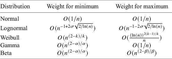
The weights for extremes (minimum and maximum) change with the sample size. Table 1 and Supplementary Text S1 summarize the asymptotic behavior of the weights for the minimum and maximum under the normal distribution with a mean $\mu$
and a SD
$\mu$
and a SD $\sigma$
, the lognormal distribution with a location parameter
$\sigma$
, the lognormal distribution with a location parameter $\mu$
and a scale parameter
$\mu$
and a scale parameter $\sigma$
, the gamma distribution with a shape parameter
$\sigma$
, the gamma distribution with a shape parameter $\alpha$
and a rate parameter
$\alpha$
and a rate parameter $\beta$
, the beta distribution with shape parameters
$\beta$
, the beta distribution with shape parameters $\alpha$
and
$\alpha$
and $\beta$
, and the Weibull distribution with a shape parameter
$\beta$
, and the Weibull distribution with a shape parameter $k$
and a scale parameter
$k$
and a scale parameter $\lambda$
as the sample size increases. The PDFs of these distributions are in Supplementary Text S1.
$\lambda$
as the sample size increases. The PDFs of these distributions are in Supplementary Text S1.
Asymptotic behavior of weights for minimum and maximum

Note: Table 1 describes the asymptotic behavior of weights for minimum and maximum under the normal distribution with a mean $\mu$
and a SD
$\mu$
and a SD $\sigma$
, the lognormal distribution with a location parameter
$\sigma$
, the lognormal distribution with a location parameter $\mu$
and a scale parameter
$\mu$
and a scale parameter $\sigma$
, the gamma distribution with a shape parameter
$\sigma$
, the gamma distribution with a shape parameter $\alpha$
and a rate parameter
$\alpha$
and a rate parameter $\beta$
, the beta distribution with shape parameters
$\beta$
, the beta distribution with shape parameters $\alpha$
and
$\alpha$
and $\beta$
, and the Weibull distribution with a shape parameter
$\beta$
, and the Weibull distribution with a shape parameter $k$
and a scale parameter
$k$
and a scale parameter $\lambda$
as the sample size increases. The probability density functions of these distributions are in Supplementary Text S1.
$\lambda$
as the sample size increases. The probability density functions of these distributions are in Supplementary Text S1.
Theoretically, as n goes to infinity, the following patterns emerge. For the normal and lognormal distributions, the weights for both the minimum and maximum converge to zero. For the Weibull and gamma distributions, the weight for the maximum converges to zero. The behavior for the minimum, however, depends on the shape parameter: it converges to zero when the shape parameter exceeds 2, remains constant when equal to 2, and diverges to infinity when less than 2. A similar pattern holds for the beta distribution, where the asymptotic weight for the minimum depends on the shape parameter $\alpha$
and for the maximum on the shape parameter
$\alpha$
and for the maximum on the shape parameter $\beta$
. In general, the weight assigned to an extreme quantile reflects its informational contribution. For distributions with light tails or low density near the boundaries, extreme values (the minimum or maximum) tend to become highly variable in large samples, contributing more noise than signal about the central characteristics of the distribution; accordingly, their weights decrease. In contrast, for distributions with heavy tails or high boundary density, extreme observations remain informative for estimating distributional parameters, and their weights decrease more slowly or even increase. This weighting scheme demonstrates how our estimators adapt automatically to the changing reliability of quantiles as the sample size grows and under different distributional assumptions.
$\beta$
. In general, the weight assigned to an extreme quantile reflects its informational contribution. For distributions with light tails or low density near the boundaries, extreme values (the minimum or maximum) tend to become highly variable in large samples, contributing more noise than signal about the central characteristics of the distribution; accordingly, their weights decrease. In contrast, for distributions with heavy tails or high boundary density, extreme observations remain informative for estimating distributional parameters, and their weights decrease more slowly or even increase. This weighting scheme demonstrates how our estimators adapt automatically to the changing reliability of quantiles as the sample size grows and under different distributional assumptions.
The theoretical possibility of infinite asymptotic weights does not impede implementation. In practice, with finite samples, all estimated weights are finite. Moreover, the weighted estimators depend only on the relative weights among quantiles. We may normalize the weights so that they sum to one without affecting the estimates, as is commonly done in matching adjusting indirect treatment comparisons and other survey sampling weighting approaches.Reference Signorovitch, Sikirica and Erder 18 , Reference Jiang, Cappelleri and Gamalo 19
3.4 Estimation procedure
To minimize the objective function, we solve for the point at which the gradient equals zero. However, due to the nonlinearity of the gradient equations and the absence of closed-form solutions, iterative optimization techniques are required. A commonly used approach is the quasi-Newton algorithm, which is well suited for nonlinear least squares problems. Additionally, the limited-memory BFGS algorithm for bound-constrained optimization (L-BFGS-B) approach can be employed to impose constraints on the parameter space.Reference Byrd, Lu and Nocedal 20 This method iteratively refines the parameter estimates until convergence criteria are satisfied. Once the parameters of the underlying distribution are estimated, the corresponding mean and variance can be computed directly.
Suppose we observe a five-number summary from data assumed to follow a beta distribution, as is common for health-related quality of life (HRQL) scores.Reference Hunger, Doring and Holle
21
In this context, $F(X,\beta )$
denotes the CDF of the beta function. The PDF, CDF, and quantile function for the beta distribution can be easily calculated in R using dbeta(), pbeta(), and qbeta(), respectively. Using an iterative optimization procedure, we can estimate the shape parameters
$F(X,\beta )$
denotes the CDF of the beta function. The PDF, CDF, and quantile function for the beta distribution can be easily calculated in R using dbeta(), pbeta(), and qbeta(), respectively. Using an iterative optimization procedure, we can estimate the shape parameters $\widehat{\alpha}$
and
$\widehat{\alpha}$
and $\widehat{\gamma}$
. The sample mean can then be calculated as
$\widehat{\gamma}$
. The sample mean can then be calculated as $\widehat{\mu}=\widehat{\alpha}/(\widehat{\alpha}+\widehat{\gamma})$
, and the sample variance can be calculated as
$\widehat{\mu}=\widehat{\alpha}/(\widehat{\alpha}+\widehat{\gamma})$
, and the sample variance can be calculated as ${\widehat{\sigma}}^2=\widehat{\alpha}\widehat{\gamma }/[{(\widehat{\alpha}+\widehat{\gamma})}^2(\widehat{\alpha}+\widehat{\gamma}+1)]$
. These formulas follow directly from the known properties of the beta distribution. Similar functionality exists in R for many other commonly used distributions, making the method broadly applicable. Additionally, software such as SAS, which also supports evaluation of density functions, CDFs, and quantile functions for a wide range of distributions, can be used to implement our approaches. This flexibility highlights the adaptability of our method to different distributional assumptions supported by standard statistical software. The R code to implement our models is available at https://github.com/xiaoyu9411/MDE.
${\widehat{\sigma}}^2=\widehat{\alpha}\widehat{\gamma }/[{(\widehat{\alpha}+\widehat{\gamma})}^2(\widehat{\alpha}+\widehat{\gamma}+1)]$
. These formulas follow directly from the known properties of the beta distribution. Similar functionality exists in R for many other commonly used distributions, making the method broadly applicable. Additionally, software such as SAS, which also supports evaluation of density functions, CDFs, and quantile functions for a wide range of distributions, can be used to implement our approaches. This flexibility highlights the adaptability of our method to different distributional assumptions supported by standard statistical software. The R code to implement our models is available at https://github.com/xiaoyu9411/MDE.
In practice, the underlying data distribution is often unknown. Following the approach of the QE method, we can select from a set of candidate parametric distributions, such as the normal, lognormal, gamma, beta, and Weibull, by identifying the one that minimizes the sum of squared residuals between the reported and theoretical quantiles. As an alternative, minimizing the sum of absolute residuals can also be employed for this distribution selection.
3.5 Percentiles for the minimum and maximum
The percentile information for minimum and maximum that the QE method used is $1/n$
and
$1/n$
and $1-(1/n)$
, respectively. However, the true percentile of the minimum lies within [0,
$1-(1/n)$
, respectively. However, the true percentile of the minimum lies within [0, $1/n$
], and the percentile of the maximum lies within
$1/n$
], and the percentile of the maximum lies within $[1-(1/n),1]$
.Reference Hyndman and Fan
22
For normal distributions, theoretical percentiles can be approximated using Blom’s equation, which assigns
$[1-(1/n),1]$
.Reference Hyndman and Fan
22
For normal distributions, theoretical percentiles can be approximated using Blom’s equation, which assigns $0.625/(n+0.25)$
for the minimum and
$0.625/(n+0.25)$
for the minimum and $(n-0.375)/(n+0.25)$
for the maximum.Reference Blom
23
For simplicity, we approximate Blom’s equation using
$(n-0.375)/(n+0.25)$
for the maximum.Reference Blom
23
For simplicity, we approximate Blom’s equation using $0.625/n$
for the minimum and
$0.625/n$
for the minimum and $1-(0.625/n)$
for the maximum. In our simulation studies (Section 4), we examined the performance of the QE method under three percentile specifications for the minimum:
$1-(0.625/n)$
for the maximum. In our simulation studies (Section 4), we examined the performance of the QE method under three percentile specifications for the minimum: $1/n$
,
$1/n$
, $0.5/n,$
and
$0.5/n,$
and $0.625/n$
(correspondingly with
$0.625/n$
(correspondingly with $1-(1/n)$
,
$1-(1/n)$
, $1-(0.5/n)$
, and
$1-(0.5/n)$
, and $1-(0.625/n)$
for the maximum), where
$1-(0.625/n)$
for the maximum), where $0.5/n$
is the midpoint of range [0,
$0.5/n$
is the midpoint of range [0, $1/n$
]. We adopted the percentile with the best performance for our proposed estimators.
$1/n$
]. We adopted the percentile with the best performance for our proposed estimators.
4 Simulation studies
4.1 Data generation and scenarios
We considered six different underlying distributions in our simulations (Figure 1): (1) a scaled beta distribution within the range $\left[0,8\right]$
with shape parameters
$\left[0,8\right]$
with shape parameters $\alpha =4$
and
$\alpha =4$
and $\beta =2$
; (2) a Weibull distribution with a shape parameter
$\beta =2$
; (2) a Weibull distribution with a shape parameter $k=1.5$
and a scale parameter
$k=1.5$
and a scale parameter $\lambda =5$
; (3) a normal distribution with a mean
$\lambda =5$
; (3) a normal distribution with a mean $\mu =5$
and a SD
$\mu =5$
and a SD $\sigma =3$
; (4) a lognormal distribution with a location parameter
$\sigma =3$
; (4) a lognormal distribution with a location parameter $\mu =1.5$
and a scale parameter
$\mu =1.5$
and a scale parameter $\sigma =0.5$
; (5) a gamma distribution with a shape parameter
$\sigma =0.5$
; (5) a gamma distribution with a shape parameter $\alpha =2.5$
and a rate parameter
$\alpha =2.5$
and a rate parameter $\beta =0.5$
; and (6) an exponential distribution with a rate parameter
$\beta =0.5$
; and (6) an exponential distribution with a rate parameter $\lambda =0.2$
. The parameter configurations were selected to ensure that the resulting means and SDs are broadly comparable across distributions while capturing a range of distributional shapes, including left-skewed, right-skewed, and symmetric forms. The corresponding values of the means and SDs are presented in Supplementary Table S1.
$\lambda =0.2$
. The parameter configurations were selected to ensure that the resulting means and SDs are broadly comparable across distributions while capturing a range of distributional shapes, including left-skewed, right-skewed, and symmetric forms. The corresponding values of the means and SDs are presented in Supplementary Table S1.
Distributions in simulation studies.

Sample sizes ranged from 30 to 1,000 in increments of 10. We also considered both least squares and least absolute deviations for selecting the underlying distributions in our proposed methods across the five candidate distributions mentioned above. For each combination of distribution, sample sizes, and distribution-selection method, we conducted 10,000 iterations under scenarios ${S}_1$
,
${S}_1$
, ${S}_2,$
and
${S}_2,$
and ${S}_3$
.
${S}_3$
.
To assess the performance of our proposed models under the conditions where theoretical asymptotic weights may diverge (as described in Section 3.3), we conducted additional simulations under ${S}_3$
with least squares method for model selection. Specifically, we examined (1) a Weibull distribution with a shape parameter
${S}_3$
with least squares method for model selection. Specifically, we examined (1) a Weibull distribution with a shape parameter $k=0.8$
and a scale parameter
$k=0.8$
and a scale parameter $\lambda =5$
; (2) a gamma distribution with a shape parameter
$\lambda =5$
; (2) a gamma distribution with a shape parameter $\alpha =0.8$
and a rate parameter
$\alpha =0.8$
and a rate parameter $\beta =5$
; (3) a beta distribution with shape parameters
$\beta =5$
; (3) a beta distribution with shape parameters $\alpha =0.8$
and
$\alpha =0.8$
and $\beta =4$
; and (4) a beta distribution with shape parameters
$\beta =4$
; and (4) a beta distribution with shape parameters $\alpha =4$
and
$\alpha =4$
and $\beta =0.8$
.
$\beta =0.8$
.
To evaluate the performance of different methods, we calculated the relative bias of the estimated mean ( $\widehat{\mu}$
) and the estimated SD (
$\widehat{\mu}$
) and the estimated SD ( $\widehat{\sigma}$
) with respect to their true values, defined as follows:
$\widehat{\sigma}$
) with respect to their true values, defined as follows:
 $$\begin{align}\mathrm{RB}\left(\widehat{\mu}\right)=\frac{1}{T}\sum \limits_{r=1}^T\frac{{\widehat{\mu}}_r-\mu }{\mu }, \mathrm{RB}\left(\widehat{\sigma}\right)=\frac{1}{T}\sum \limits_{r=1}^T\frac{{\widehat{\sigma}}_r-\sigma }{\sigma },\end{align}$$
and the relative mean squared error (RMSE) as follows:
 $$\begin{align}\mathrm{RMSE}\left(\widehat{\mu}\right)=\frac{\frac{1}{T}\sum \limits_{r=1}^T{\left({\widehat{\mu}}_r-\mu \right)}^2}{\frac{1}{T}\sum \limits_{r=1}^T{\left({\overline{X}}_r-\mu \right)}^2}, \mathrm{RMSE}\left(\widehat{\sigma}\right)=\frac{\frac{1}{T}\sum \limits_{r=1}^T{\left({\widehat{\sigma}}_r-\sigma \right)}^2}{\frac{1}{T}\sum \limits_{r=1}^T{\left({S}_r-\sigma \right)}^2},\end{align}$$
where $T$
is the number of iterations,
$T$
is the number of iterations, $\overline{X}$
stands for the true sample mean, and
$\overline{X}$
stands for the true sample mean, and $S$
represents the true sample SD.
$S$
represents the true sample SD.
4.2 Results
4.2.1 Choice of percentiles for the minimum and maximum
We examined the performance of the QE method under three percentile specifications for the minimum: $1/n$
,
$1/n$
, $0.5/n$
, and
$0.5/n$
, and $0.625/n$
(correspondingly with
$0.625/n$
(correspondingly with $1-\left(1/n\right)$
,
$1-\left(1/n\right)$
, $1-\left(0.5/n\right)$
, and
$1-\left(0.5/n\right)$
, and $1-\left(0.625/n\right)$
for the maximum) under
$1-\left(0.625/n\right)$
for the maximum) under ${S}_3$
(Supplementary Figures S1–S4). When the underlying distributions are scaled,
${S}_3$
(Supplementary Figures S1–S4). When the underlying distributions are scaled, $\mathrm{beta}(4,2)$
,
$\mathrm{beta}(4,2)$
, $\mathrm{normal}(5,3)$
,
$\mathrm{normal}(5,3)$
, $\mathrm{lognormal}(1.5,0.5)$
, and
$\mathrm{lognormal}(1.5,0.5)$
, and $\mathrm{gamma}(2.5,0.5)$
using
$\mathrm{gamma}(2.5,0.5)$
using $0.625/n$
and
$0.625/n$
and $0.5/n$
as percentiles for minimum significantly reduced both bias and RMSEs for estimates of the mean and SD compared to
$0.5/n$
as percentiles for minimum significantly reduced both bias and RMSEs for estimates of the mean and SD compared to $1/n$
. Under
$1/n$
. Under $\mathrm{Weibull}\;(1.5,5)$
, both
$\mathrm{Weibull}\;(1.5,5)$
, both $0.625/n$
and
$0.625/n$
and $0.5/n$
slightly improved relative bias for the mean and SD and RMSEs in SD for large sample sizes (Supplementary Figure S5). Under
$0.5/n$
slightly improved relative bias for the mean and SD and RMSEs in SD for large sample sizes (Supplementary Figure S5). Under $\mathrm{exponential}(0.2)$
, both
$\mathrm{exponential}(0.2)$
, both $0.625/n$
and
$0.625/n$
and $0.5/n$
reduced relative bias for the mean and SD and RMSEs in SD for small sample sizes (Supplementary Figure S6). Given the small differences in performance between
$0.5/n$
reduced relative bias for the mean and SD and RMSEs in SD for small sample sizes (Supplementary Figure S6). Given the small differences in performance between $0.5/n$
and
$0.5/n$
and $0.625/n$
, we prioritized theoretical alignment with Blom’s method, adopting
$0.625/n$
, we prioritized theoretical alignment with Blom’s method, adopting $0.625/n\kern0.24em$
as the percentile for the minimum and
$0.625/n\kern0.24em$
as the percentile for the minimum and $1-\left(0.625/n\right)$
as the percentile for the maximum.
$1-\left(0.625/n\right)$
as the percentile for the maximum.
4.2.2 Comparison of different methods
Results under scenario ${S}_3$
are presented in Figures 2–7. Both the wQE and MDE methods outperformed the QE method across all six underlying distributions, with a particular advantage for SD estimates where a dramatic reduction in RMSEs was observed. The two proposed methods exhibited similar performance in general, but the MDE method showed slightly higher relative bias compared to the wQE method in some cases. The method by Luo et al. and Shi et al. yielded biased estimates for the scaled
${S}_3$
are presented in Figures 2–7. Both the wQE and MDE methods outperformed the QE method across all six underlying distributions, with a particular advantage for SD estimates where a dramatic reduction in RMSEs was observed. The two proposed methods exhibited similar performance in general, but the MDE method showed slightly higher relative bias compared to the wQE method in some cases. The method by Luo et al. and Shi et al. yielded biased estimates for the scaled $\mathrm{beta}(4,2)$
,
$\mathrm{beta}(4,2)$
, $\mathrm{gamma}(2.5,0.5)$
,
$\mathrm{gamma}(2.5,0.5)$
, $\mathrm{Weibull}(1.5,5)$
, and
$\mathrm{Weibull}(1.5,5)$
, and $\mathrm{exponential}(0.2)$
distributions. For the
$\mathrm{exponential}(0.2)$
distributions. For the $\mathrm{normal}(5,3)$
distribution, our methods provided mean estimates comparable to Luo’s optimal method for the mean, but exhibited slightly higher bias for the SD when sample sizes were smaller than 100 compared to Shi’s optimal method for the SD. The RMSEs for both the mean and SD are comparable to the optimal methods. Under the
$\mathrm{normal}(5,3)$
distribution, our methods provided mean estimates comparable to Luo’s optimal method for the mean, but exhibited slightly higher bias for the SD when sample sizes were smaller than 100 compared to Shi’s optimal method for the SD. The RMSEs for both the mean and SD are comparable to the optimal methods. Under the $\mathrm{lognormal}(1.5,0.5)$
distribution, our methods slightly overestimated the mean and SD for sample sizes below 200 and showed higher RMSE compared to Shi’s method, which was optimal for this distribution. For the remaining distributions, both wQE and MDE outperformed the optimal methods based on the normal distribution. When sample size was less than 100, the bias for our methods remained within 10% for
$\mathrm{lognormal}(1.5,0.5)$
distribution, our methods slightly overestimated the mean and SD for sample sizes below 200 and showed higher RMSE compared to Shi’s method, which was optimal for this distribution. For the remaining distributions, both wQE and MDE outperformed the optimal methods based on the normal distribution. When sample size was less than 100, the bias for our methods remained within 10% for $\mathrm{exponential}(0.2)$
and within 4% for other distributions; for larger sample sizes, our methods generated nearly unbiased estimates with low RMSE.
$\mathrm{exponential}(0.2)$
and within 4% for other distributions; for larger sample sizes, our methods generated nearly unbiased estimates with low RMSE.
Performance of estimators under $\mathrm{Beta}(\min =0,\max =8,\alpha =4,\beta =2)$
in
$\mathrm{Beta}(\min =0,\max =8,\alpha =4,\beta =2)$
in ${S}_3$
. Least squares method was used for distribution selection for wQE and MDE.
${S}_3$
. Least squares method was used for distribution selection for wQE and MDE.

Performance of estimators under $\mathrm{Normal}(5,3)$
in
$\mathrm{Normal}(5,3)$
in ${S}_3$
. Least squares method was used for distribution selection for wQE and MDE.
${S}_3$
. Least squares method was used for distribution selection for wQE and MDE.

Performance of estimators under $\mathrm{Lognormal}(1.5,0.5)$
in
$\mathrm{Lognormal}(1.5,0.5)$
in ${S}_3$
. Least squares method was used for distribution selection for wQE and MDE.
${S}_3$
. Least squares method was used for distribution selection for wQE and MDE.

Performance of estimators under $\mathrm{Gamma}(2.5,0.5)$
in
$\mathrm{Gamma}(2.5,0.5)$
in ${S}_3$
. Least squares method was used for distribution selection for wQE and MDE.
${S}_3$
. Least squares method was used for distribution selection for wQE and MDE.

Performance of estimators under $\mathrm{Weibull}(1.5,5)$
in
$\mathrm{Weibull}(1.5,5)$
in ${S}_3$
. Least squares method was used for distribution selection for wQE and MDE.
${S}_3$
. Least squares method was used for distribution selection for wQE and MDE.

Performance of estimators under Exponential $(0.2)$
in
$(0.2)$
in ${S}_3$
. Least squares method was used for distribution selection for wQE and MDE.
${S}_3$
. Least squares method was used for distribution selection for wQE and MDE.

The results in ${S}_1$
were consistent with the findings from scenario
${S}_1$
were consistent with the findings from scenario ${S}_3$
(Supplementary Figures S7–S12). wQE and MDE also outperformed the QE method. The pattern of performance against the optimal methods was similar. In
${S}_3$
(Supplementary Figures S7–S12). wQE and MDE also outperformed the QE method. The pattern of performance against the optimal methods was similar. In ${S}_1$
, our methods exhibited the highest precision for the scaled
${S}_1$
, our methods exhibited the highest precision for the scaled $\mathrm{beta}(4,2)$
,
$\mathrm{beta}(4,2)$
, $\mathrm{gamma}(2.5,0.5)$
,
$\mathrm{gamma}(2.5,0.5)$
, $\mathrm{Weibull}(1.5,5)$
, and
$\mathrm{Weibull}(1.5,5)$
, and $\mathrm{exponential}(0.2)$
distributions.
$\mathrm{exponential}(0.2)$
distributions.
Results under scenario ${S}_2$
are presented in Supplementary Figures S13–S18. The optimal methods for normal distribution yielded biased estimates for the scaled
${S}_2$
are presented in Supplementary Figures S13–S18. The optimal methods for normal distribution yielded biased estimates for the scaled $\mathrm{beta}(4,2)$
,
$\mathrm{beta}(4,2)$
, $\mathrm{gamma}(2.5,0.5)$
,
$\mathrm{gamma}(2.5,0.5)$
, $\mathrm{Weibull}(1.5,5)$
, and
$\mathrm{Weibull}(1.5,5)$
, and $\mathrm{exponential}(0.2)$
distributions. The wQE and MDE methods performed similarly to the QE method overall. When the sample size was small, all three methods overestimated the mean and SD for the scaled
$\mathrm{exponential}(0.2)$
distributions. The wQE and MDE methods performed similarly to the QE method overall. When the sample size was small, all three methods overestimated the mean and SD for the scaled $\mathrm{beta}(4,2)$
,
$\mathrm{beta}(4,2)$
, $\mathrm{normal}(5,3)$
,
$\mathrm{normal}(5,3)$
, $\mathrm{gamma}(2.5,0.5)$
,
$\mathrm{gamma}(2.5,0.5)$
, $\mathrm{Weibull}(1.5,5)$
, and
$\mathrm{Weibull}(1.5,5)$
, and $\mathrm{exponential}(0.2)$
distributions and underestimated the mean and SD for the
$\mathrm{exponential}(0.2)$
distributions and underestimated the mean and SD for the $\mathrm{lognormal}(1.5,0.5)$
distribution. For large sample sizes, the estimates were nearly unbiased in most of distributions, with the exception of slight underestimation of the SD for the
$\mathrm{lognormal}(1.5,0.5)$
distribution. For large sample sizes, the estimates were nearly unbiased in most of distributions, with the exception of slight underestimation of the SD for the $\mathrm{lognormal}(1.5,0.5)$
distribution and a slight overestimation of the SD for the
$\mathrm{lognormal}(1.5,0.5)$
distribution and a slight overestimation of the SD for the $\mathrm{Weibull}(1.5,5)$
and
$\mathrm{Weibull}(1.5,5)$
and $\mathrm{exponential}(0.2)$
distributions. For the
$\mathrm{exponential}(0.2)$
distributions. For the $\mathrm{normal}(5,3)$
distribution, the RMSE of the mean for our methods was higher than that of QE for n < 600 but became lower as the sample size increased. For the
$\mathrm{normal}(5,3)$
distribution, the RMSE of the mean for our methods was higher than that of QE for n < 600 but became lower as the sample size increased. For the $\mathrm{exponential}(0.2)$
distribution with
$\mathrm{exponential}(0.2)$
distribution with $n<200$
, our methods yielded substantially lower relative bias and RMSE for the SD than the QE method.
$n<200$
, our methods yielded substantially lower relative bias and RMSE for the SD than the QE method.
In distribution selection, the proportion of correct selection increases with sample size in general (Supplementary Figures S19–S21). Our methods achieved higher correct selection rates for the normal distribution in ${S}_2$
(60%–100%) compared to the QE method (50%–90%). For the
${S}_2$
(60%–100%) compared to the QE method (50%–90%). For the $\mathrm{Weibull}(1.5,5)$
distribution, our methods achieved correct selection rates of 50%–80% in
$\mathrm{Weibull}(1.5,5)$
distribution, our methods achieved correct selection rates of 50%–80% in ${S}_1$
and 40%–70% in
${S}_1$
and 40%–70% in ${S}_3$
, whereas the QE method rarely selected the correct distribution (under 20% in
${S}_3$
, whereas the QE method rarely selected the correct distribution (under 20% in ${S}_1$
and
${S}_1$
and ${S}_3$
). For the exponential distribution, our methods achieved higher correct selection rates than the QE method in both
${S}_3$
). For the exponential distribution, our methods achieved higher correct selection rates than the QE method in both ${S}_1$
and
${S}_1$
and ${S}_3$
when the sample size was below 400. The QE method demonstrated a higher proportion of correct selections for the lognormal and gamma distributions in
${S}_3$
when the sample size was below 400. The QE method demonstrated a higher proportion of correct selections for the lognormal and gamma distributions in ${S}_1$
and
${S}_1$
and ${S}_3$
. wQE, MDE, and QE showed comparable overall performance in other scenarios. We also evaluated the use of least absolute deviations for distribution selection but found it did not improve performances and reduced the correct selection rate for the normal distribution (Supplementary Figures S22–S42); therefore, the least squares criterion was adopted for our models.
${S}_3$
. wQE, MDE, and QE showed comparable overall performance in other scenarios. We also evaluated the use of least absolute deviations for distribution selection but found it did not improve performances and reduced the correct selection rate for the normal distribution (Supplementary Figures S22–S42); therefore, the least squares criterion was adopted for our models.
Under distributions where the theoretical asymptotic weights may diverge (Supplementary Figures S43–S46), our methods generally achieved lower relative bias and RMSE for both the mean and SD than the QE approach across nearly all scenarios. For large sample sizes, the proposed estimators produced nearly unbiased estimates across the examined distributions. Overall, the two proposed methods performed similarly, although the wQE method demonstrated slightly lower relative bias and RMSE than the MDE method in certain cases.
5 Illustrative example
We illustrated our proposed methods using the data from an individual participant data meta-analysis that investigated the diagnostic accuracy of Patient Health Questionaire-9 (PHQ-9), which was used as an illustrative example in the QE paper by McGrath et al.Reference McGrath, Zhao and Steele
15
,
Reference Thombs, Benedetti and Kloda
24
For each study, they provided the sample mean, sample SD, and five-number summaries (Supplementary Table S2). The PHQ-9 is a self-administered questionnaire that assesses the severity of depressive symptoms, with scores ranging from 0 to 27. Higher scores indicate more severe depression. Prior research has found that PHQ-9 scores tend to be right-skewed.Reference Tomitaka, Kawasaki and Ide
25
,
Reference Kocalevent, Hinz and Brahler
26
Although the original meta-analysis focused on diagnostic accuracy using bivariate modeling, the availability of IPD allowed for the calculation of the true sample means and SDs for each study. This provided an opportunity to benchmark the performance of conversion methods against actual values, serving as a validation exercise within a real-world research context. Additionally, the IPD enabled us to generate all five-number summaries, illustrating our method’s application across different scenarios under ${S}_1$
,
${S}_1$
, ${S}_2$
, and
${S}_2$
, and ${S}_3$
. Using our proposed methods and other existing methods mentioned above, we meta-analyzed PHQ-9 scores from 58 primary studies. Given the bounded and right-skewed distribution of PHQ-9 scores, we normalized the five-number summaries by dividing each value by 27. This transformation constrained the values within a range of 0–1, making them suitable for modeling using the beta distribution. After estimating the parameter estimation of the chosen distribution, we rescaled the derived sample means and SDs by multiplying them by 27, thereby reverting to the original scale of PHQ-9 scores.
${S}_3$
. Using our proposed methods and other existing methods mentioned above, we meta-analyzed PHQ-9 scores from 58 primary studies. Given the bounded and right-skewed distribution of PHQ-9 scores, we normalized the five-number summaries by dividing each value by 27. This transformation constrained the values within a range of 0–1, making them suitable for modeling using the beta distribution. After estimating the parameter estimation of the chosen distribution, we rescaled the derived sample means and SDs by multiplying them by 27, thereby reverting to the original scale of PHQ-9 scores.
We used a random-effects model for meta-analysis with between-study variance estimated using restricted maximum likelihood.Reference Langan, Higgins and Jackson
27
Table 2 presents the meta-analysis of PHQ-9 scores, using both true sample means/SDs and estimates derived from quantiles across different methods under ${S}_1$
,
${S}_1$
, ${S}_2$
, and
${S}_2$
, and ${S}_3$
. The benchmark results, obtained from the true sample means and SDs, yielded a pooled PHQ-9 estimate of 6.53 (95% CI: 5.97, 7.09), with a between-study variance (τ) of 2.13 and
${S}_3$
. The benchmark results, obtained from the true sample means and SDs, yielded a pooled PHQ-9 estimate of 6.53 (95% CI: 5.97, 7.09), with a between-study variance (τ) of 2.13 and ${I}^2$
of 97.4%. Under
${I}^2$
of 97.4%. Under ${S}_1$
, the QE method produced a pooled estimate of 7.65 (95% CI: 7.08, 8.23), representing the largest deviation from the benchmark. In contrast, the wQE and MDE methods yielded estimates of 6.50 (95% CI: 5.93, 7.07) and 6.51 (95% CI: 5.93, 7.09), which were closer to the value obtained from the true sample means and SDs. All methods yielded slightly higher heterogeneity estimates compared to the benchmark (
${S}_1$
, the QE method produced a pooled estimate of 7.65 (95% CI: 7.08, 8.23), representing the largest deviation from the benchmark. In contrast, the wQE and MDE methods yielded estimates of 6.50 (95% CI: 5.93, 7.07) and 6.51 (95% CI: 5.93, 7.09), which were closer to the value obtained from the true sample means and SDs. All methods yielded slightly higher heterogeneity estimates compared to the benchmark ( $\tau$
: 2.15–2.33;
$\tau$
: 2.15–2.33; ${I}^2$
: 97.5%–98.5%). The QE method exhibited a predominant selection of the beta distribution (93.1%), while the wQE and MDE methods demonstrated a balanced selection between Weibull distribution and beta distribution (Supplementary Table S3). In
${I}^2$
: 97.5%–98.5%). The QE method exhibited a predominant selection of the beta distribution (93.1%), while the wQE and MDE methods demonstrated a balanced selection between Weibull distribution and beta distribution (Supplementary Table S3). In ${S}_2$
, the Luo/Shi’s method showed a considerable underestimation (5.68; 95% CI: 5.06, 6.29). The QE, wQE, and MDE methods all showed better performance, with MDE (6.60; 95% CI: 5.90, 7.30) being closest to the benchmark. These three methods exhibited higher estimates of
${S}_2$
, the Luo/Shi’s method showed a considerable underestimation (5.68; 95% CI: 5.06, 6.29). The QE, wQE, and MDE methods all showed better performance, with MDE (6.60; 95% CI: 5.90, 7.30) being closest to the benchmark. These three methods exhibited higher estimates of ${I}^2$
(97.9%–98.1%) and
${I}^2$
(97.9%–98.1%) and $\tau$
(2.58–2.68) compared to the benchmark. The distribution selection patterns in
$\tau$
(2.58–2.68) compared to the benchmark. The distribution selection patterns in ${S}_2$
were diverse across all methods, with no single distribution dominating (Supplementary Table S4). Under
${S}_2$
were diverse across all methods, with no single distribution dominating (Supplementary Table S4). Under ${S}_3$
, the Luo/Shi’s method demonstrated the poorest performance (5.97; 95% CI: 5.36, 6.58). The QE method showed the closest results to the benchmark (6.59; 95% CI: 6.03, 7.15), with wQE and MDE producing slightly higher estimates (6.65; 95% CI: 6.11, 7.20 and 6.71; 95% CI: 6.16, 7.25, respectively). Heterogeneity statistics for these methods were consistent with those derived from the true sample means and standard deviations (
${S}_3$
, the Luo/Shi’s method demonstrated the poorest performance (5.97; 95% CI: 5.36, 6.58). The QE method showed the closest results to the benchmark (6.59; 95% CI: 6.03, 7.15), with wQE and MDE producing slightly higher estimates (6.65; 95% CI: 6.11, 7.20 and 6.71; 95% CI: 6.16, 7.25, respectively). Heterogeneity statistics for these methods were consistent with those derived from the true sample means and standard deviations ( $\tau$
: 2.07–2.13;
$\tau$
: 2.07–2.13; ${I}^2$
: 97.1%–97.9%). wQE and MDE showed strong preference for beta distribution (82.8% and 84.5%), while the QE method showed comparable selection rates for Weibull (43.1%) and beta (41.4%) distributions (Supplementary Table S5). Given the stable performance of wQE and MDE methods across all scenarios, they are valuable for skewed data conversion.
${I}^2$
: 97.1%–97.9%). wQE and MDE showed strong preference for beta distribution (82.8% and 84.5%), while the QE method showed comparable selection rates for Weibull (43.1%) and beta (41.4%) distributions (Supplementary Table S5). Given the stable performance of wQE and MDE methods across all scenarios, they are valuable for skewed data conversion.
Meta-analysis results on PHQ-9 scores based on different conversion methods

Note: Luo/Shi (Wan) are the optimal methods based on normal distributions. QE refers to the quantile estimation method. wQE is the weighted QE method. MDE is the minimum distance estimator.
6 Discussion
In meta-analysis, researchers frequently need to convert quantile-based summaries into means and standard deviations to incorporate studies that reported different types of summary statistics. In this paper, we highlight the limitations of existing approaches and propose weighted estimators for estimating sample means and SDs from quantiles commonly reported in literatures. These estimators facilitate meta-analyses that integrate studies reporting quantiles with those reporting means and SDs. In addition, our methods are readily applicable to a wide range of underlying distribution for which PDFs and CDFs can be computed using standard software.
Closed-form formulas for optimal estimators of sample mean and SD exist for normalReference Wan, Wang and Liu
8
–
Reference Shi, Luo and Weng
10
and lognormal distributions.Reference Shi, Tong and Wang
14
In our simulations, while the proposed estimators exhibited slightly larger biases and RMSEs than these optimal methods for small sample sizes, their performance was comparable for larger sample sizes under most cases in ${S}_1$
and
${S}_1$
and ${S}_3$
. For other skewed distributions examined, our methods outperformed the normal-based optimal methods in both relative bias and RMSE. The QE method assumes equal weighting across quantiles, but quantiles vary in reliability due to their varying variances. For example, the median is a robust statistic with a bounded influence function,Reference David and Nagaraja
28
whereas the minimum and maximum are more variable due to their sensitivity to extreme values. This motives the use of inverse-variance weighting in our proposed estimators. Consistent with this intuition, our simulations show that the weighted approaches provide improved accuracy over the QE method, particularly when the minimum and maximum are included. The two proposed methods performed similarly across almost all scenarios. Given their comparable performance, we recommend the wQE estimator for routine use due to its more intuitive theoretical foundation, particularly for clinicians and applied researchers.
${S}_3$
. For other skewed distributions examined, our methods outperformed the normal-based optimal methods in both relative bias and RMSE. The QE method assumes equal weighting across quantiles, but quantiles vary in reliability due to their varying variances. For example, the median is a robust statistic with a bounded influence function,Reference David and Nagaraja
28
whereas the minimum and maximum are more variable due to their sensitivity to extreme values. This motives the use of inverse-variance weighting in our proposed estimators. Consistent with this intuition, our simulations show that the weighted approaches provide improved accuracy over the QE method, particularly when the minimum and maximum are included. The two proposed methods performed similarly across almost all scenarios. Given their comparable performance, we recommend the wQE estimator for routine use due to its more intuitive theoretical foundation, particularly for clinicians and applied researchers.
Although meta-analyses often focus on group differences, for which the sampling distribution of the mean difference typically approaches normality via the Central Limit Theorem, even when the underlying data are nonnormal or skewed, the summary statistics themselves are typically reported separately by group, particularly for secondary or exploratory endpoints.Reference Moher, Hopewell and Schulz
29
The underlying data within each group may be substantially skewed. Furthermore, there is often a need to meta-analyze the means of raw outcome values themselves, not just differences, for example, when establishing reference ranges.Reference Siegel, Murad and Riley
30
Existing methods, especially those relying on analytical formulas, are generally limited to commonly reported summaries (e.g., ${S}_1$
,
${S}_1$
, ${S}_2,$
and
${S}_2,$
and ${S}_3$
). However, with the growing adoption of distributed learning,Reference Kirienko, Sollini and Ninatti
31
it is increasingly feasible to obtain more detailed quantile data from participating sites while still preserving data privacy. In such settings, our proposed approaches are versatile and can accommodate a variety of underlying distributions and any set of quantiles, including commonly reported summaries or more detailed percentile data. We also recommend that future studies report additional percentiles beyond the minimum and maximum (e.g., the 5th and 95th percentiles), as extreme values may reflect outliers and are often less informative.
${S}_3$
). However, with the growing adoption of distributed learning,Reference Kirienko, Sollini and Ninatti
31
it is increasingly feasible to obtain more detailed quantile data from participating sites while still preserving data privacy. In such settings, our proposed approaches are versatile and can accommodate a variety of underlying distributions and any set of quantiles, including commonly reported summaries or more detailed percentile data. We also recommend that future studies report additional percentiles beyond the minimum and maximum (e.g., the 5th and 95th percentiles), as extreme values may reflect outliers and are often less informative.
Our work has several limitations. First, we require the number of parameters ( $J$
) in the underlying distribution be less than or equal to the number of available quantiles (
$J$
) in the underlying distribution be less than or equal to the number of available quantiles ( $k$
). When
$k$
). When $J>k$
, the number of parameters exceeds the number of available quantiles, making them not estimable. However, since
$J>k$
, the number of parameters exceeds the number of available quantiles, making them not estimable. However, since $k$
is usually at least 3 in practical applications, our methods are broadly applicable to most parametric distributions, which generally require fewer than three parameters. Second, our simulation studies focus on sample sizes larger than 30, which reflect typical study sizes in meta-analyses. However, in certain contexts, such as research on rare diseases, meta-analyses may include studies with very small sample sizes (e.g., n
$k$
is usually at least 3 in practical applications, our methods are broadly applicable to most parametric distributions, which generally require fewer than three parameters. Second, our simulation studies focus on sample sizes larger than 30, which reflect typical study sizes in meta-analyses. However, in certain contexts, such as research on rare diseases, meta-analyses may include studies with very small sample sizes (e.g., n $\approx$
10). Because our methods rely on iterative optimization rather than closed-form equations, the performance can become unstable under such conditions. Third, we evaluated both least squares and least absolute deviations for distribution selection, but the correct selection rate remained below 50% for some distributions at small sample sizes likely due to the limited number of quantiles available. Hence, developing improved model selection criteria is an important direction for future work. We recommend conducting sensitivity analyses to assess how alternative distributional assumptions influence the meta-analysis results.
$\approx$
10). Because our methods rely on iterative optimization rather than closed-form equations, the performance can become unstable under such conditions. Third, we evaluated both least squares and least absolute deviations for distribution selection, but the correct selection rate remained below 50% for some distributions at small sample sizes likely due to the limited number of quantiles available. Hence, developing improved model selection criteria is an important direction for future work. We recommend conducting sensitivity analyses to assess how alternative distributional assumptions influence the meta-analysis results.
In conclusion, our methods offer a flexible framework for estimating sample mean and SD from quantiles across a variety of underlying distributions, facilitating more comprehensive meta-analysis that incorporate different summary formats. Researchers may either specify a plausible distribution based on subject-matter knowledge or use data-driven model selection to guide estimation.
Author contributions
Conceptualization: T.T., H.C.; Data curation: X.T.; Formal analysis: X.T., T.T., X.Z., H.C.; Methodology: X.T., T.T., X.Z., H.C.; Software: X.T., X.Z., H.C.; Supervision, H.C.; Validation: X.T., T.T., X.Z., H.C.; Visualization: X.T., T.T., X.Z.; Writing—original draft: X.T.; Writing—review and editing: X.T., T.T., X.Z., H.C.
Competing interest statement
X.Z. and H.C. are employed by Pfizer and may own stocks of their company. However, all contents in this article are strictly educational, instructive, and methodological, not involving any real medicinal intervention.
Data availability statement
The data supporting the illustrative example are included in the Supplementary Material. The R code implementing the proposed methods can be accessed at https://url.uk.m.mimecastprotect.com/s/Go1SCL866TPY5oX9FBfqSyHdaa?domain=zenodo.org.
Funding statement
X.T.’s research was supported by the Research Development Fund (Grant No. RDF2401022) at Xi’an Jiaotong-Liverpool University. T.T.’s research was supported by the General Research Fund of Hong Kong (HKBU12300123 and HKBU12303421) and the Initiation Grant for Faculty Niche Research Areas of Hong Kong Baptist University (RC-FNRA-IG/23-24/SCI/03).
Supplementary material
To view supplementary material for this article, please visit http://doi.org/10.1017/rsm.2026.10090.


 Open access