


1. Introduction
Marine outlet glaciers, or tidewater glaciers, widespread around Greenland, in the Arctic, in Alaska and the Antarctic Peninsula, terminate in fjords with nearly vertical calving fronts that are often fully grounded (e.g. Vieli, Reference Vieli2015). Long-term observations of several tidewater glaciers in Alaska (e.g. Plafker and Miller, Reference Plafker and Miller1957; Post, Reference Post1975; Pfeffer and others, Reference Pfeffer, Humphrey, Amadei, Harper and Wegmann2000) and more recent remote-sensing observations in the Arctic, Greenland and Antarctica (e.g. Gardner and others, Reference Gardner2013; Moon and others, Reference Moon2014) indicate that they exhibit a ‘tidewater glacier cycle’ (Post, Reference Post1975). During the start of this cycle, their termini typically slowly advance or remain quiescent, the cycle ends with rapid retreat into deeper waters. The rapid retreat is typically associated with mass loss at the termini either because of submarine melting (e.g. Motyka and others, Reference Motyka, Hunter, Echelmeyer and Connor2003; Sutherland and others, Reference Sutherland2019) or calving (e.g. Vieli and others, Reference Vieli, Jania and Kolondra2002). This cycle has a very rich behaviour depending on the magnitudes of the mass loss.
Iceberg calving is a complex process, and a universal ‘calving law’ that could relate glacier characteristics to iceberg calving characteristics (e.g. timing, frequency and size) remains elusive. It is also unclear how atmospheric and oceanic conditions affect calving and how their effects can be accounted for. Adding to the complexity, in situ (Amundson and others, Reference Amundson2010) and remote-sensing (Joughin and others, Reference Joughin, Shean, Smith and Floricioiu2020) observations suggest that the ice mélange adjacent to the glaciers calving front modulates iceberg calving and terminus migration. Iken (Reference Iken1977), Hughes (Reference Hughes1992), van der Veen (Reference van der Veen1996), Brown and others (Reference Brown, Meier and Post1982), Vieli and others (Reference Vieli, Funk and Blatter2001), Benn and others (Reference Benn, Warren and Mottram2007) and Nick and others (Reference Nick, van der Veen, Vieli and Benn2010) among many others have considered various mechanisms and parameterisations that can explain observed tidewater glacier calving. Several widely used approaches to represent calving in flow models assume that icebergs calve when ice thickness reaches the flotation condition (Vieli and others, Reference Vieli, Funk and Blatter2001) or when surface crevasses widely observed on such glaciers propagate to the glacier bed (Benn and others, Reference Benn, Warren and Mottram2007; Nick and others, Reference Nick, van der Veen, Vieli and Benn2010).
The rapid retreat of glaciers’ termini into deeper waters during the retreat phase of the tidewater glacier cycle has been interpreted as an indication of ‘marine ice-sheet instability’ – a hypothesis proposed by Weertman (Reference Weertman1974) for unconfined marine ice sheets, which requires the flux at the grounding line (the location where ice starts to float) to be an increasing function of ice thickness. However, considering a laterally confined marine outlet glacier Schoof and others (Reference Schoof, Devis and Popa2017) have shown that for such a configuration the ice flux is no longer an increasing function of ice thickness if the effects of lateral shear caused by the lateral confinement is larger than the effects of basal shear. As a result, the deepening of the bed underneath the glacier does not imply that it is unconditionally unstable, and the ‘marine ice-sheet instability’ hypothesis is not suitable to interpret the observed behaviour, i.e. the bed slope alone is not indicative of the glacier stability; the observed retreat can be driven by variations in the external forcings (e.g. surface ablation or submarine melting) not co-incident with the retreat itself.
Bassis and Walker (Reference Bassis and Walker2012) have proposed that the rapid retreat of tidewater glaciers could be caused by shear failure of terminus ice cliffs after they reach a critical thickness threshold determined by the ice strength. If the bed of the glacier is up-sloping, i.e. shallows in the direction of its flow, this implies a runaway process termed ‘marine ice-cliff instability’ (Pollard and others, Reference Pollard, DeConto and Alley2015). An approach that calving can be described as ice failure when the ice effective stress reaches the yield strength has been developed by Bassis and Ultee (Reference Bassis and Ultee2019). In their approach, ice is treated as a viscoplastic material and ice thickness at the calving front is at a critical value determined by the yield strength. Using a more complex, composite ice rheology which allows simulation of the ice brittle failure, Bassis and others (Reference Bassis, Berg, Crawford and Benn2021) performed numerical simulations of an unconfined marine outlet glacier and concluded that the ice-thickness gradient determines whether the glacier terminus can experience an unstoppable retreat and that the presence of ice mélange has strong effects on it.
The study presented here builds on studies by Schoof and others (Reference Schoof, Devis and Popa2017) and Bassis and Ultee (Reference Bassis and Ultee2019) and explores the behaviour of laterally confined marine outlet glaciers with grounded calving front, i.e. without a floating tongue. It aims to establish fundamental relationships between the glacier characteristics (e.g. terminus position and the rate of its migration, ice flux, ice thickness, basal and lateral conditions), and environmental conditions (e.g. mélange backstress) for several different treatments of the calving process. These relationships can shed light on the observed behaviour of marine outlet glaciers. Comparing the calving-front ice flux or its migration rate predicted by these relationships to the observations will help to determine which of the calving parameterisations, if any, can be used as ‘calving laws’ and under which circumstances.
The paper is organised as follows: the glacier flow model is described in Section 2. Section 3 describes derivations of the relationships at the calving front (between ice flux, ice thickness and other glacier and environmental parameters; and between the calving-front migration rate and glacier parameters) and conditions of stability of steady-state configurations. The performance of these relationships for different calving rules and in the presence or absence of mélange is described in Section 4.
2. Model description
This study considers a laterally confined marine outlet glacier that terminates on the bed, i.e. does not develop a floating ice tongue (Fig. 1). The case of a laterally confined ice stream or a glacier floating into a confined ice shelf has been considered by Haseloff and Sergienko (Reference Haseloff and Sergienko2018). The model used here is vertically integrated (e.g. MacAyeal, Reference MacAyeal1989; Schoof and others, Reference Schoof, Devis and Popa2017; Bassis and Ultee, Reference Bassis and Ultee2019; Sergienko and Wingham, Reference Sergienko and Wingham2022) and laterally averaged (e.g. Nick and others, Reference Nick, van der Veen, Vieli and Benn2010; Hindmarsh, Reference Hindmarsh2012; Sergienko, Reference Sergienko2012; Pegler, Reference Pegler2016; Haseloff and Sergienko, Reference Haseloff and Sergienko2018). It amalgamates features from three models: the lateral confinement and calving conditions based on the flotation condition and the water-filled crevasse depth used in a model by Schoof and others (Reference Schoof, Devis and Popa2017); calving conditions based on yield strength used in a model by Bassis and Ultee (Reference Bassis and Ultee2019) and the effects of basal topography considered in a model by Sergienko and Wingham (Reference Sergienko and Wingham2022). In addition, it accounts for possible effects of backstress provided by mélange or already calved icebergs.
Model geometry: b – bed elevation (b < 0), h – ice thickness, x d – the ice divide location, x c – the calving-front location.

2.1. Governing equations and boundary conditions
The momentum and mass balances of the marine outlet glacier are


where x and t denote partial derivatives with respect to x and t, respectively, u(x) is the depth- and width-averaged ice velocity, h(x) is the ice thickness, b(x) is the bed elevation (negative below sea level and positive above sea level), A is the ice stiffness parameter (assumed to be constant), n is the exponent of Glen's flow law, g is the acceleration due to gravity, τ w is the lateral shear, τ b is the basal shear, x d = 0 is the location of the ice divide, x c is the location of the calving front and $\dot a$ is the net accumulation/ablation rate (positive for accumulation). Basal sliding τ b is treated as a power-law function

where C b is the basal shear parameter and m is the sliding exponent (e.g. Budd and others, Reference Budd, Keage and Blundy1979; Fowler, Reference Fowler1981), and

where C w is a lateral shear stress parameter (taken here to be a constant C w = 21+1/n) and W is the width of the glacier (e.g. Raymond, Reference Raymond1996; Schoof and others, Reference Schoof, Devis and Popa2017).
Boundary conditions at the divide x d are


At the calving front x c there are two conditions:


where the first condition (5a) is the stress condition, and the second condition (5b) describes the calving condition. It has been suggested (e.g. Amundson and others, Reference Amundson2010) that mélange or earlier calved icebergs can provide backstress to the terminus. The term τ m on the right-hand side of (5a) represents the effects of mélange backstress. This form of the stress condition is similar to the stress conditions at the grounding line obtained by Schoof and others (Reference Schoof, Devis and Popa2017) and by Haseloff and Sergienko (Reference Haseloff and Sergienko2018) for the case of a laterally confined ice shelf, where backstress or buttressing is caused by the lateral confinement of the ice shelf and is determined by the ice-shelf properties and processes (e.g. sub-ice-shelf melting). In that case and in the case of the bed-terminating calving front considered here, backstress τ m acts to reduce the stress at the calving front (or the grounding line). Resolving the mélange dynamics and establishing an explicit functional form of τ m is beyond the scope of this study; so the only assumption made about τ m is that it could vary spatially, i.e. τ m = τ m(x). Studies by Robel (Reference Robel2017) and Burton and others (Reference Burton, Amundson, Cassotto, Kuo and Dennin2018) and others focused on details of mélange behaviour.
2.2. Calving rules
In the absence of a universal ‘calving law’, many different conditions have been considered as calving rules. They include conditions on the magnitude of ice thickness, stress, flux or migration rate at the calving front. This study focuses on three calving rules that are based on the magnitude of ice thickness. The first is a widely used rule based on the flotation thickness (e.g. Vieli and others, Reference Vieli, Funk and Blatter2001); it assumes that an iceberg calves if the calving-front ice thickness is at flotation, i.e.

This condition is termed FL throughout the text.
The second is based on an idea that calving takes place when surface crevasses filled with water propagate to the glacier bed. Here, its formulation follows Schoof and others (Reference Schoof, Devis and Popa2017), which is based on the model proposed by Nick and others (Reference Nick, van der Veen, Vieli and Benn2010):

where d w is the crevasse water depth. The present study limits itself to the outlet glacier configuration without floating tongues, and consequently considers the case of d w/ (− b) ≥ 1/2,

where

(Schoof and others, Reference Schoof, Devis and Popa2017, eqn (1i)). This condition is referred to as CD.
The third adopts a calving rule proposed by Bassis and Ultee (Reference Bassis and Ultee2019) which is also based on the critical value of the ice thickness

where τ y is the yield strength of ice. This condition is referred to as YS. Qualitatively, the three ‘calving laws’ (6–9) are similar in a sense that they impose a condition on the ice thickness at the calving front.
The problem (1–5) with τ m = 0 in (5a) and the flotation condition (6) as the condition (5b) also describes the behaviour of the laterally confined ice streams or outlet glaciers flowing into an unconfined ice shelf – a configuration characteristic of ice streams flowing into the Filchner-Ronne Ice Shelf with no pinning points downstream. For ice shelves with lateral extent significantly larger than the lateral extent of individual ice streams feeding them the stress-regime downstream of their grounding lines is similar to the one of an unconfined ice shelf.
3. Conditions at the calving front
This section describes derivations of relationships at the calving front: a relationship between ice flux and ice thickness (13); the rate of the calving-front migration (16) and conditions of stability of the steady-state configurations (24). To derive these relationships, we consider the ice-flow stress regime in which the dominant balance is between the driving stress and lateral and basal shear stresses, and the longitudinal-stress divergence is smaller than these terms. A similar regime has been considered by Schoof and others (Reference Schoof, Devis and Popa2017) and Bassis and Ultee (Reference Bassis and Ultee2019).
Here, we rely on results of the analysis of Sergienko and Wingham (Reference Sergienko and Wingham2022), who showed that if the longitudinal-stress divergence is small compared to other terms of the momentum balance through the length of an unconfined glacier, it also remains small compared to other terms in the vicinity of the calving front (the grounding line, in their case). A boundary layer, which one might expect to form from scaling considerations, is very weak due to specifics of the sliding law and non-linearity of ice flow (Sergienko and Wingham, Reference Sergienko and Wingham2022, Appendix A). The applicability of these results to a configuration considered here are confirmed with numerical solutions of a steady-state version of the model (1–5) (Figs 3, 6 and A1, A2), and the results will be discussed in detail in Section 4.
Following Sergienko and Wingham (Reference Sergienko and Wingham2022), we reformulate the approximate problem (1–5) in terms of ice thickness h and the ice flux q = uh instead of the ice velocity u. It is


where the stress condition was obtained by using,

and rewriting (10a) in a form

Equation (10d) is the relationship between the ice flux and the ice thickness at the calving front; it is valid for both steady-state and time-evolving configurations of a glacier. For configurations evolving with time $q_x = \dot a- h_t$ and (10d) becomes

where the fact that q > 0 at x c (i.e. the glacier flows towards its calving front) was taken into account.
3.1. Calving-front migration rate
The rate of the calving-front advance or retreat is determined by taking the total time-derivative of the calving thickness condition (10e)

where $\dot x_{\rm c}$ is the rate of the calving-front migration and h cx is the gradient of the ice thickness at the calving front, i.e. the gradient of the right-hand side expressions of the calving rules FL, CD and YS. Rearranging terms gives

Combining (14) and (12) with (13) and rearranging terms gives

Expressions (10d) and (16) are general forms for the ice flux at the calving front and the rate of its migration for all calving rules is based on ice thickness at the calving front.
For specific forms of the calving rule, expressions for the migration rate are obtained by using the following expressions for h cx:

for FL,

for CD, and

for YS, respectively.
In the case of FL

where the term δb x/(1 − δ) was neglected in the denominator.
In the case of CD, expression for the rate of the calving-front migration is

and in the case of YS, it is

3.2. Steady-state flux, position and stability
In steady state $q_x = \dot a$ , and the flux at the calving front is determined by

The steady-state positions of the calving front are determined through the addition of the calving condition (5b) and the fact that in steady state ${q( x_{\rm c}) = \int _0^{x_{\rm c}}\dot a {\rm d}x}$ ; their values are determined as the roots of the transcendental equation (23), of which there may be none, one or several.
To determine the stability conditions of the steady-state configurations, we follow a standard approach of linear stability analysis (e.g. Schoof, Reference Schoof2012; Sergienko and Wingham, Reference Sergienko and Wingham2019, Reference Sergienko and Wingham2022). It is algebraically complex and its details are described in Appendix A. Its results show that the calving front is stable if

or

and is unstable if the sign in the first inequality in (24a) and (24b) is reversed, provided that at x = x c

where


and q and h = h c are steady-state values at the calving front, b xx is the bed curvature, $\dot a_x$ is the gradient of the net ablation/accumulation rate, τ mx is the gradient of the mélange backstress and h cx are defined by (17–19) for the corresponding calving conditions FL-YS. If condition (25a) is not satisfied, no inferences about stability can be made without explicitly solving a perturbation problem (A6). For the calving condition FL, the stability condition is (24a), as h x < h cx ensures that the glacier remains grounded upstream of the calving front.
Expressions (13–24) are general expressions for laterally confined outlet glaciers with their calving fronts situating on the bedrock or flowing into an unconfined (or very wide) ice shelf (with the condition FL) which longitudinal stress divergence is much smaller than other components of their momentum balance. In circumstances where the momentum balance is dominated by either basal shear (wider glaciers with stronger basal resistance) or by lateral shear (narrow glaciers with weak basal resistance), these expressions are simplified as the corresponding terms can be neglected (e.g. either C w ≈ 0 or C b ≈ 0). The expressions are also simplified in the absence of backstress from mélange (τ m = 0). Note that all expressions derived in this section are specific to the chosen forms of the basal and lateral shears (2) and (3), respectively. For different forms, for instance one based on the Coulomb friction law (Tsai and others, Reference Tsai, Stewart and Thompson2015), these expressions will have different forms.
4. Effects of calving rules and mélange backstress
To get insights how a marine glacier behaves under different calving rules and whether mélange is present or absent in front of it, we consider a glacier with the width W = 10 km, with the ice stiffness parameter A = 2.11 × 10⁻²⁵ Pa−3 s−1 (corresponding to ice temperature ≈ −15°C), the sliding coefficient C = 7.6 × 10⁶ Pa m−1/3 s1/3 (a value used in a number of studies (e.g. Schoof, Reference Schoof2007; Schoof and others, Reference Schoof, Devis and Popa2017; Bassis and Ultee, Reference Bassis and Ultee2019; Sergienko and Wingham, Reference Sergienko and Wingham2022), the sliding exponent m = 1/n = 1/3, and the bed topography b(x) = b 0 + b a cos πx/L, where b 0 = −500 m, b a = 250 m, L = 500 km. This shape has down- and up-sloping parts, allowing us to investigate glacier configurations with calving fronts located on different slopes. For the calving rule CD, d w/ − b = 1/2. For the calving rule YS the yield stress is τ y = 100 kPa. When mélange backstress is present, its magnitude is τ m = 107 Pa m for all calving rules – a threshold for mélange jamming, found by Burton and others (Reference Burton, Amundson, Cassotto, Kuo and Dennin2018). Additionally, a value of τ m = 108 Pa m is considered for the FL rule. For the other calving rules there are no steady-state configurations with this magnitude of τ m on the down-sloping part of the bed.
Although the calving flux, migration rate and stability conditions depend on parameters such as the glacier width W, sliding parameters C and m, bed topography, ice stiffness, etc., we do not investigate their influence here, leaving comprehensive sensitivity analyses to the future studies. To verify the accuracy of the approximate analytical expressions derived in the previous section, we compare them to results of numerical solutions, which are obtained with the finite-element solver Comsol (COMSOL, 2022). The steady-state solutions are obtained by solving an optimisation problem using a minimisation procedure based on the bound optimisation by quadratic approximation optimisation algorithm (Powell, Reference Powell2009). In all simulations, the grid resolution is spatially variable: it is 200 m through 95% of the length of the domain, and 1 m in the 5% closest to the calving-front position x c. The time-dependent solutions of (1) with boundary conditions (4–5) are obtained on domains with a moving boundary, the calving front. This is done using an arbitrary Lagrangian–Eulerian method (Donea and others, Reference Donea, Huerta, Ponthot and Rodríguez-Ferran2017). The calving front moves with velocity (15), where all terms are computed by the model.
4.1. Effects of calving rules
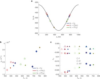
In order to assess how the choice of a calving rule affects the behaviour of a marine outlet glacier, we consider a situation where mélange is absent, i.e. τ m = 0. Figure 2a illustrates the steady-state calving-front positions for three calving rules FL-YS. All positions on the down-sloping bed (x < 500 km) are obtained with the accumulation rate $\dot a = 30$ cm a−1, and all positions on the up-sloping bed are obtained with $\dot a = 10$
 cm a−1. Circle, square and triangle symbols indicate results of numerical simulations solving problem (1–5) with the corresponding calving rules FL-YS; diamond symbols indicate solutions of the approximate analytic expressions (23). The largest difference between the numerical simulations and approximate values are 160 m for the calving-front positions x c, which ranges from 195 to 772 km, and 27 cm for the ice thickness at the calving front h c, which ranges from 465 to 622 m. The close agreement between the results of full numerical solutions and approximate expressions indicate that the approximate expressions accurately capture the behaviour of marine outlet glaciers simulated with the numerical model that accounts for all terms in the momentum balance (1).
(a) Calving-front positions; (b) the relationship between ice flux and ice thickness and (c) ice-thickness gradient at the calving-front position computed for different calving laws. Circle, square and triangle symbols are numerical solutions, diamond symbols are analytic expressions. In panel (a) diamonds are roots of transcendental equations (23) together with the corresponding expressions for h c FL-YS and in panel (b) diamonds are expressions (23). The solutions of the approximate expressions and numerical solutions overlap. In panel (c) colours are the same as in panels (a) and (b), symbols indicate different terms of expression (12) computed numerically. Two sets of the same symbols with the same colour correspond to the calving-front positions on the down- and up-sloping parts of the bed. In all experiments the ice flow is from left to right.

The relationship between the steady-state calving-front ice flux and ice thickness is illustrated in Fig. 2b. For the chosen set of parameters, the calving rule YS results in a calving front on deeper parts of the bed and a larger calving-front thickness than the calving rules based on flotation condition FL and the depth of the water-filled crevasses CD. Although for this calving rule CD the steady-state calving-front positions are on the shallowest parts of the bed, and have smaller ice thickness, the calving flux at the location on the up-sloping bed is larger than for the case of FL.
Bassis and others (Reference Bassis, Berg, Crawford and Benn2021) have investigated the behaviour of an unconfined marine outlet glacier (i.e. τ w = 0), and concluded that the ice thickness gradient is a controlling factor in stability of marine outlet glaciers with tall ice cliffs. In circumstances where the longitudinal stress gradient is small, the ice-thickness gradient is determined by other components of the momentum balance (12). Figure 2c illustrates contributions of various terms at the calving-front position. For the chosen set of parameters, the term associated with the basal shear (term II) is dominant. The magnitude of this term is the smallest for the calving rule YS (green symbols).
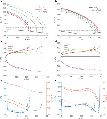
The steady-state configurations of marine outlet glaciers with terminus positions are shown in Fig. 2a, in Fig. 3a for the locations on the down-sloping part of the bed (x < 500 km) and in Fig. 3b for the locations on the up-sloping part of the bed. The configuration corresponding to the calving rule YS has the calving front farther downstream on the down-sloping bed than the calving-front positions for the other two calving rules (green line in Fig. 3a). Correspondingly, the glacier with this calving rule is thicker than the glaciers with the other calving rules. The calving-front positions on the up-sloping part of the bed (Fig. 3b) are closer to each other for all calving rules, and the glaciers’ shape do not greatly differ from one another.
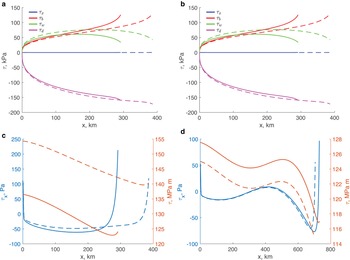
(a) and (b) Glacier surface elevation, S and bed elevation B (black line) for steady-state calving-front positions on down-sloping and up-sloping bed. Black dashed line indicates sea level. (c) and (d) The components of the momentum balance (1a) for the calving rule FL (blue line in panels (a) and (b)). τ x is the first term and τ d is the last term on the left-hand side of (1a); τ b and τ w are defined by (2) and (3). (e) and (f) show the τ x (left axis) and τ = 2 A −1/nh|u x|1/n−1u x (right axis) computed in numerical solutions. Note different units on left vertical axes in panels (c)–(f).

Figures 3c and 3d show the terms of the momentum balance (1a) for the calving rule FL (the corresponding glaciers’ configurations are shown with blue lines in Figs 3a and 3b). For the chosen parameter values, the longitudinal-stress gradient τ x (the first term of (1a)) is significantly smaller than the other terms of the momentum balance. The basal and lateral shear, τ b (2) and τ w (3), respectively, have similar magnitudes through the length of the glacier (green and red lines in Figs 3c, d), and together balance the driving stress τ d (the last term of (1a)). The basal shear becomes larger closer to the calving front, although the lateral shear is non-negligible at the calving front. For the calving rules FL and CD the momentum balance is similar – the longitudinal-stress gradient is significantly smaller than the other components; and the magnitudes of the lateral shear reduce closer to the calving front, but remain non-negligible. As Figs 3e, f illustrate, the longitudinal-stress divergence (blue lines, left axes) reduces away from the calving front, indicating the presence of a boundary layer. However, its maximum magnitude at least two and a half orders of magnitudes smaller than magnitudes of other components of the momentum balance (Figs 3c, d). The smallness of the divergence of the longitudinal stress does not imply the smallness of the longitudinal stress itself (red lines, right axis in Figs 3e, f). Its values at the calving front are determined by the stress boundary condition (5a). For other calving rules the terms of the momentum balances exhibit very similar behaviour (Figs A1 and A2). These results justify the assumption of the negligible longitudinal-stress divergence through the length of the glacier, including the vicinity of the calving front, and a non-negligible longitudinal stress itself, made at the onset of this study.
To investigate the role of calving rules in the dynamic behaviour of the marine outlet glacier, we consider periodic variations in the accumulation rate

where $\dot a_0$ is the same as the steady-state value (0.3 m a−1), $\Delta \dot a = 0.5$
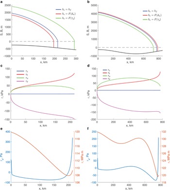
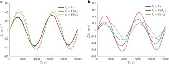
 m a−1 and T = 5000 years (the same period used by Bassis and Ultee, Reference Bassis and Ultee2019). The initial conditions are steady-state configurations with the calving-front positions on the down-sloping part of the bed (Fig. 3a). Figure 4a shows the rate of the calving-front migration for different calving rules. For the chosen parameters, the calving rules FL (blue lines) and CD (red lines) result in a similar dynamic response of the calving front with amplitudes of advance and retreat on the order of 20–30 m a−1. In the case of the calving rule YS (green line) the magnitude of advance and retreat is larger, ~ 40 m a−1, and the maximum and minimum rates are achieved ~ 200 years later than those for other calving rules. The close agreement between the approximate analytic values (20–22) (dotted-dashed lines in Fig. 4a) and numerical values (solid lines in Fig. 4a), with the difference <0.5 m a−1 for all calving rules suggests that (20–22) accurately describe the calving-front migration rates for all calving rules.
Rate of the calving-front migration $\dot x_{\rm c}$ (m a−1) in the absence of mélange. (a) Solid lines are numerically simulated values, dotted-dashed lines are values computed with the analytic expressions (20–22). (b) The difference between numerically and analytically computed values of $\dot x_{\rm c}$
 (m a−1).

4.2. Effects of mélange backstress
The effects of mélange were emulated by applying τ m = 107 Pa m for steady-state configurations. For all calving rules, the calving-front positions were located on deeper parts of the bed (filled symbols in Fig. 5a) compared to the calving-front positions in the absence of mélange (open symbols in Fig. 5a). Regardless of the calving-front location on the down- or up-sloping part of the bed, the ice thickness at the calving front is larger in the presence of mélange (filled symbols in Fig. 5b). The corresponding ice flux is larger for the calving rules FL and CD (red and blue symbols in Fig. 5b), but it is slightly smaller for the calving rule CD on the up-sloping bed (green symbols in Fig. 5b). For the chosen parameters, the presence of mélange does not alter contributions of various terms to the ice-thickness gradient at the calving front (filled symbols in Fig. 5c). The second term in (12) associated with the basal shear (II) has the largest magnitude, but it is smaller than that in the absence of mélange (open symbols in Fig. 5c).
Effects of mélange on the calving-front position, flux and ice-thickness gradient. Panels are the same as in Fig. 2; filled symbols are values in the presence of mélange backstress, small symbols correspond to τ m = 107 Pa m for all calving rules, large symbols correspond to τ m = 108 Pa m for the calving rule FL; open symbols are the same as in Fig. 2.

The glaciers with terminus positions on the down-sloping part of the bed are larger (i.e. thicker and longer) in the presence of mélange with τ m = 107 Pa m (dashed lines in Fig. 6a). The difference is largest for the calving rule YS for which, in the presence of mélange, the calving-front position is almost 100 km downstream of the calving-front position in the absence of mélange (green lines in Fig. 6a), and the glacier is ~ 500 m thicker. For τ m = 108 Pa m the steady-state configuration on the down-sloping bed exists only for the calving rule FL (blue dotted-dashed line). In this case, the calving front is ~ 150 km downstream of its position for τ m = 107 Pa m and the glacier is ~ 700 m thicker. On the up-sloping part of the bed, for τ m = 107 Pa m the calving-front positions are upstream when mélange is present (dashed lines in Fig. 6b). However, the difference between the calving-front positions is within 25 km; consequently, the glacier configurations are not significantly different with or without mélange. For τ m = 108 Pa m and the calving rule FL (blue dotted-dashed line) the calving front is the farthest upstream, and the glacier is overall thinner by ~ 500 m compared to configurations with either no mélange or smaller τ m.
Effects of mélange on the steady-state configurations and momentum balance. Panels are the same as in Fig. 2; dashed lines are values in the presence of mélange backstress τ m = 107 Pa m for all calving rules, dash-dotted lines for τ m = 108 Pa m for the calving rule FL; solid lines are the same as in Fig. 3. Note different units on left vertical axes in panels (c)–(f).

The momentum balance is not significantly altered by the effects of mélange backstress (Figs 6c, d, A1a, b, A2a, b). The basal and lateral shears equally balance the driving stress. The presence of mélange and large τ m tend to reduce the magnitude of the longitudinal-stress divergence even further (Figs 6e, f, A1c, d, A2c, d).
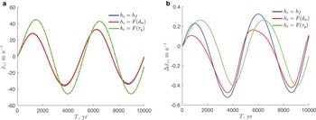
The dynamic response of the glacier to periodic changes in accumulation rate described by (27) in the presence of mélange is quantitatively similar to the case when it is absent. For the calving rules FL and CD the rates of the calving-front migration have similar magnitudes (blue and red lines in Fig. 7a). In the absence of mélange (solid lines in Fig. 7a), the magnitudes are larger by ~ 1.5 m a−1. For the calving rule YS (green lines in Fig. 7a), the magnitudes of the calving-front migration rate is larger in the presence of mélange (dashed line); and its maximum is ~ 150 years later than that in the absence of mélange (solid line). Figure 7b shows the difference between the migration rates computed numerically and the expressions (20–22). The small magnitudes of the difference indicates that approximate analytic expressions accurately describe the dynamic behaviour of marine outlet glaciers simulated with the full numerical model.
Effects of mélange on the rate of the calving-front migration $\dot {x}_{\rm c}$ (m a−1). (a) Numerically computed $\dot {x}_{\rm c}$
 (m a−1); dashed lines are values in the presence of mélange backstress τ m = 107 Pa m for all calving rules, dashed-dotted line is for the FL calving rule with τ m = 108 Pa m; solid lines are the same as in Fig. 4a. Double-dashed-dotted lines are values computed with the analytic expressions (20–22). (b) The difference between numerically and analytically computed values (Eqns (20–22)) in the presence of mélange, dashed-dotted line corresponds to the calving rule FL with τ m = 108 Pa m.

The simulated magnitudes of the calving-front migration are substantially smaller than the observed values. This is a result of a combination of used parameters, values of which either have been used in previous idealised studies (e.g. the sliding coefficient C, the period of temporal variability T) or have been chosen such that steady-state configurations with the calving-front positions on the down- and up-sloping parts of the bed can exist for the three calving rules considered here. The close agreement of the approximate expressions derived in this study with the results of the full numerical model suggests the validity of these expressions for a parameter range similar to values of realistic glaciers as long as the glacier conditions satisfy assumptions underlying the derived expressions.
5. Discussion
In this study, we have investigated the behaviour of laterally confined marine outlet glaciers that do not form a floating tongue. Previous studies by Schoof and others (Reference Schoof, Devis and Popa2017) and Bassis and Ultee (Reference Bassis and Ultee2019) considered similar configurations using different forms of ‘calving laws’ – one, FL, assumes that calving happens when the glacier terminus reaches flotation condition; another, CD, assumes that calving happens when the water-filled crevasses reach a critical depth; another, YS, assumes that calving happens when the terminus ice thickness reaches a critical value, which is determined by the yield stress of ice. The common feature of these calving rules is that they impose a condition on ice thickness at the calving front. Using this commonality, we have derived analytic expressions for the ice flux at the terminus assuming both steady-state and time evolving conditions, (23) and (13), respectively. For dynamic (i.e. time-evolving) glaciers we have determined the rate of the calving-front migration (16), and for steady-state glaciers we have derived stability conditions (24). These conditions are significantly more complex than those associated with the marine ice-sheet instability hypothesis (Weertman, Reference Weertman1974; Schoof, Reference Schoof2012). In the case of the laterally confined marine outlet glacier, the ice flux at the calving front is an implicit function of ice thickness (23). Thus, similar to other geometric (Gudmundsson and others, Reference Gudmundsson, Krug, Durand, Favier and Gagliardini2012; Haseloff and Sergienko, Reference Haseloff and Sergienko2018; Pegler, Reference Pegler2018; Sergienko and Wingham, Reference Sergienko and Wingham2022) and dynamic (Sergienko and Wingham, Reference Sergienko and Wingham2019) configurations the marine ice-sheet instability hypothesis is not generally applicable to the marine outlet glaciers as has been suggested by Schoof and others (Reference Schoof, Devis and Popa2017), i.e. their steady-state configurations can be stable and unstable on down- or up-sloping beds depending on combinations of the glacier parameters.
The derived expressions depend on the bed geometry – its elevation, slope (b x) and curvature (b xx); the glacier width (W); parameters of the basal and lateral shears (C w, C b and m, respectively); the ice stiffness parameter (A) and the Glen's flow-law exponent (n); the ice thickness at the calving front determined by a specific calving rule h c and the corresponding parameters it depends on (e.g. the depth of water-filled crevasses (d w), the yield stress (τ y)) and the calving-thickness gradient (h cx); the accumulation rate ($\dot a$ ) and the accumulation-rate gradient ($\dot a_x$
 ); the mélange backstress (τ m) and the backstress gradient (τ mx). The dependence on such a large number of parameters and their complex combination suggest that marine outlet glaciers can exhibit a diverse range of behaviours. The majority of these parameters are either directly observable (e.g. the glacier geometry, the absence or presence of water and its depth) or can be inferred from observations using various techniques (e.g. inverse methods and machine learning). Consequently, the derived expressions can be used to get insights into the observed wide range of behaviours of marine outlet glaciers (e.g. Moon and others, Reference Moon2014).
To limit the scope, this study has focused on two aspects – the effects of calving rules and mélange backstress. For the chosen sets of parameters, the glacier's steady-state configurations and their dynamic behaviour, specifically the rate of the calving-front migration, have larger differences for the calving rule based on the yield stress YS than those for the calving rules based on the flotation condition FL or the water-filled crevasse depth CD (Figs 2–4). These differences are larger for glaciers with the calving-front positions located on the down-sloping part of the bed than on the up-sloping parts of the bed. In the presence of mélange stress at its critical value of jamming (τ m = 107 Pa m), the steady-state glacier configurations for the three calving rules are larger (i.e. thicker and longer) for the glacier with the calving front on the down-sloping part of the bed and slightly smaller for the glaciers on up-sloping part of the bed (Figs 6a, b). The largest differences are for the calving rule YS. For stronger mélange backstress (τ m = 108 Pa m), there are no steady-state configurations on the down-sloping part of the bed for calving rules CD and YS for the same values of the accumulation/ablation rate $\dot a$ . For the calving rule FL, the steady-state calving-front positions are located on deeper parts on both down- and up-sloping sections of the bed (blue dotted-dashed lines in Figs 6a, b). In the presence of mélange the longitudinal-stress divergence, which is already smaller than other components of the momentum balance tends to be even smaller (Figs 6e, f, A1c, d, A2c, d). It should be emphasised, however, that the shape of the bed b(x) exhibits a strong control on the glacier dynamics (Sergienko and Wingham, Reference Sergienko and Wingham2022), and the presence of basal undulations on the spatial scales of several tens of ice thicknesses will result in stronger effects of basal topography than those obtained in the example of the long-wave topography considered here.
The calving rule YS based on the yield stress is associated with the marine ice-cliff instability hypothesis proposed by Pollard and others (Reference Pollard, DeConto and Alley2015). According to it, the glaciers on the up-sloping beds are structurally unstable because of the ice strength is not sufficient enough to support cliffs taller than a threshold value. The derived stability condition (24) with the corresponding expressions for h c (9) and h cx (19) indicates circumstances under which a steady-state configuration of a marine outlet glacier is stable or unstable to small perturbations. A tall cliff on a bed with the retrograde slope does not imply instability as suggested by the marine ice cliff instability hypothesis (Pollard and others, Reference Pollard, DeConto and Alley2015). As already mentioned, the stability conditions derived here depend on a complex combination of numerous parameters. These conditions provide insights into which outlet-glacier configurations are more or less prone to it. One of parameters they depend on is the divergence of mélange stress (τ mx) (26b). This suggests that in addition to other specific conditions of the glacier, like lateral and basal shears, the details of the melange stress regime (i.e. its magnitude and whether it is extensional or compressional, e.g. due to the winds or ocean flow) affect the stability of a steady-state configuration.
A numerical study by Bassis and others (Reference Bassis, Berg, Crawford and Benn2021) investigated the behaviour of an unconfined outlet glacier with a tall cliff. In that study, ice was treated as a material with a composite rheology in order to simulate the ice brittle failure. Bassis and others (Reference Bassis, Berg, Crawford and Benn2021) concluded that the controlling factors are the ice-thickness gradient and the ice inflow velocity. As expression (12) indicates, the ice-thickness gradient depends on the bed slope and the basal and lateral shears, with the latter being a function of the glacier width. As boundary conditions, Bassis and others (Reference Bassis, Berg, Crawford and Benn2021) imposed ice velocity and kept the ice thickness constant at the upstream end of the glacier. These conditions are equivalent to prescribing the mass flux into the glacier. As our results show, the steady-state calving-front positions, as well as the rate of the calving-front migration are determined by the ice flux at the calving front, which is the total mass flux transported by the glacier, i.e. the mass flux at its upstream and mass flux accumulated through its length. Thus, the expressions derived here provide physical insights into why the numerical results of Bassis and others (Reference Bassis, Berg, Crawford and Benn2021) depend on the ice-thickness gradient.
The derived expressions of the rate of calving-front migration can be used to gain understanding of the processes and parameters that control it. As expressions (16–22) indicate, the rate of the calving-front migration is determined by the local properties at the calving front, as well as ice flux at the calving front, which is the integral property – the mass flux gained through the glacier surface through its length. According to the mass balance (1b), ice flux at the calving front is

Therefore, the rate of the calving-front migration $\dot x_{\rm c}$ (16), which depends on q(x c), depends non-linearly on the horizontal extent of the glacier, i.e. the calving-front position x c. Hence, there is a non-linear feedback between the rate of the calving-front migration rate and calving-front position.
Expressions (16–22) suggest that the rate of calving-front migration may exhibit different behaviour for different calving rules. These expressions depend on parameters specific to individual glaciers, e.g. their width, bed elevation and its curvature, sliding parameters and specifics of calving. As a result, the migration rates observed on individual glaciers are not informative of the migration rates in other locations or under different environmental conditions, even though they have been used in such a way in large-scale ice-sheet models (e.g. DeConto and Pollard, Reference DeConto and Pollard2016).
The results of this study have several limitations. They have been obtained using a width-averaged flow model, therefore, the effects of ice-flow transverse variability (e.g. Gudmundsson, Reference Gudmundsson2003; Sergienko, Reference Sergienko2012) are not accounted for. All derivations are done under an assumption that the divergence of the longitudinal stress is smaller than other terms of the momentum balance – the basal and lateral shears and the driving stress. The derivations are performed for specific forms of lateral and basal shears. Additionally, these results have been obtained under assumptions underlying the shallow shelf/stream approximation (MacAyeal, Reference MacAyeal1989). The limits of these assumptions set additional limits of applicability of these results.
6. Conclusions
The time-evolving and steady-state configurations and stability of steady states of laterally confined marine-outlet glaciers without floating tongues depend on a large number of geometric parameters, basal and lateral conditions, the presence or absence of mélange at their calving fronts and specifics of a calving rule applied at the calving front. There is a non-linear feedback between the rate of the calving-front migration and the flux at the calving-front position, and consequently the calving-front position itself. The close agreement of derived expressions with numerical simulations indicate that these expressions can be used to shed light on the observed behaviour of marine outlet glaciers. It also suggests that such observations can be used to determine which calving rules and which glaciological settings better describe the calving process.
Acknowledgements
I would like to thank Scientific Editors Jonathan Kingslake and Ralf Greve, Doug Brinkerhoff and two anonymous referees for thoughtful comments and useful suggestions that greatly improved the manuscript. This study is supported by an award NA18OAR4320123 from the National Oceanic and Atmospheric Administration, U.S. Department of Commerce. The statements, findings, conclusions and recommendations are those of the author and do not necessarily reflect the views of the National Oceanic and Atmospheric Administration or the U.S. Department of Commerce.
APPENDIX A.
A Linear stability analysis
A linearised perturbation problem is constructed by considering small perturbations of the order of a small parameter σ around the steady state

where the steady-state solutions are denoted by $\hat {}$ , and substituting these expressions to (10) and collecting terms of O(σ)


where


Substituting (A3a) to (A2b) results in a second-order PDE for $\tilde h$

which admits solutions in a form

Substituting it to (A4) leads to an eigenvalue problem for Λ


where


As in other studies of marine ice sheets with the longitudinal stress divergence being smaller than other components of the momentum balance (Schoof, Reference Schoof2012; Sergienko and Wingham, Reference Sergienko and Wingham2022), it is not possible to determine the magnitude of Λ without solving the eigen-value problem; however, it is possible to establish its sign, which determines stability of a steady state. If all Λ are negative than small perturbations $\tilde h$ , $\tilde q$
 and $\tilde x_{\rm c}$
 reduce with time, and the steady-state configuration is stable. If at least one value of Λ is positive than small perturbations increase with time and the steady-state configuration is unstable.
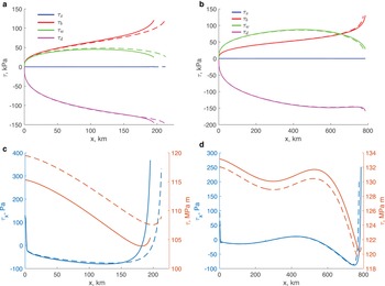
Components of the momentum balance (1a) for the calving rule CD computed in numerical solutions. Dashed lines are values in the presence of mélange backstress τ m = 107 Pa m. Note different units on left vertical axes.

Components of the momentum balance (1a) for the calving rule YS for the calving rule CD computed in numerical solutions. Dashed lines are values in the presence of mélange backstress τ m = 107 Pa m. Note different units on left vertical axes.

The eigenvalue problem (A6) includes the eigenvalue Λ in its boundary condition and is similar to one considered by Sergienko and Wingham (Reference Sergienko and Wingham2022). Their analysis and re-formulation of (A6) as a Sturm–Liouville problem directly applies here. Taking into account ${\tilde q = -\Lambda \int _0^x\tilde h {\rm d}x^\prime }$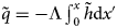 , dividing both sides of (A6c) and rearranging terms gives

where

The sign of the first term in square brackets on the right-hand side is positive when A 2 is positive. This is due to the fact that, the eigenfunction $\tilde h$ corresponding to the largest value of Λ has no zeros in accordance with Theorem 1 of Linden (Reference Linden1991), provided A 2 > 0; and consequently the term ${{\int _0^{\hat x_{\rm c}}\tilde h{\rm d}x^\prime }/{\tilde h}}$
 is positive. The sign of the denominator $\hat h_x-h_{{\rm c}x}$
 is known for a given calving rule (17–19) and a particular steady-state configuration (12). Thus, the sign of Λ is determined by the sign of the numerator: it is negative if the numerator is positive. That implies that a steady state is stable if


and is unstable if


provided

If (A14) is not satisfied, no inferences about stability of a steady-state configurations can be made without solving the eigenvalue problem (A6).


 Open access