


1. Introduction
A popular conjecture in scholarship on American politics holds that performing well in Iowa and New Hampshire helps candidates secure the U.S. presidential nomination through positive spillover effects on performance in subsequent primary elections. The first-in-the-nation status of these states would direct media coverage, public attention, and campaign donations toward winning candidates, helping their chances in states that hold their contests later in the season and prompting weaker candidates to drop out due to a lack of such resources (Polsby, Reference Polsby1983; Adams, Reference Adams, Orren and Polsby1987; Bartels, Reference Bartels1988; Winebrenner and Goldford, Reference Winebrenner and Goldford2010; Christenson and Smidt, Reference Christenson and Smidt2012).
There was a time when scholars thought pre-primary insider endorsements were more important for success in the primaries (e.g. Cohen et al., Reference Cohen, Karol, Noel and Zaller2008), but more recent successes by outsider candidates such as Obama and Trump have led scholars to change their view (e.g. Cohen et al., Reference Cohen, Karol, Noel and Zaller2016). The widespread acceptance of this success-breeds-success effect in U.S. politics rationalizes the very actions that would drive it: if doing well is instrumental because public attention and donations go to those who do well and exceed expectations, then the allocation of public attention and money to top performers makes sense. The conjecture also explains the historical front-loading behavior of states seeking to increase their influence on candidate selection.
What is the empirical basis for the conjecture? Our literature review finds a broad consensus within empirical political science: of the 22 peer-reviewed studies conducted since the 1980s that discuss an “Iowa or New Hampshire effect,” only 3 report finding mixed results or no such effect. Most of these studies operationalize performance in the first states by focusing on winning (x/22) or on overall vote share (y/22) as driving momentum effects.Footnote 1 While overall vote share is the most common independent variable, winning, the focus of this article, is nonetheless central in the literature. For instance, Collingwood et al. (Reference Collingwood, Barreto and Donovan2012) write “(...) candidate viability is a driving factor in informing the candidate chance component of vote choice and that momentum gained through primary victories is the surest path to viability” (p. 238). Bartels (Reference Bartels1988) argues winning is more important than vote share because it creates more media attention: “Given the interest of the news media in simple, dramatic stories, the best way to attract the sort of attention that might lead to widespread public support was to win primaries. Candidates who did win primaries–the earlier and oftener the better–found that these primary successes, magnified by the news media, sometimes generated more new support than any amount of money could buy” (p. 25). And Adkins and Dowdle (Reference Adkins and Dowdle2000) echo this argument: “Although the winner here [New Hampshire] does not always claim the nomination, the media are usually quick to point out that every presidential general election winner (with the exception of Bill Clinton in 1992) won this race” (p. 257).
This broad consensus notwithstanding, a key problem faced by all studies on doing well in the early states is that candidates and campaigns have features that impact their performance in the same direction in all states but cannot be perfectly measured. As a result, performance in Iowa must be positively correlated to performance in later states, also after controlling for observable candidate traits. Some candidates may, for example, have more popular policy proposals, be better looking, be a better public speaker, have a campaign team with better connections to the media or funders, leading to more media attention and early funds, which results in additional voters in the initial and later states. Variables such as these are hard to measure empirically but will typically confound the relationship between candidate success in early states and performance in later ones. Regardless of whether there truly is a first-in-the-nation effect, there will be many cases in which the ultimate nominee won either Iowa or New Hampshire, a statistical regularity that is readily quoted by political commentators in support of its existence (Skelley, Reference Skelley2019).
Addressing this problem requires a setting wherein performance in a given state is orthogonal to the candidate’s electoral potential. Such a setting is provided by a regression discontinuity design. By focusing on winning, as opposed to vote share, we can compare narrow wins with narrow losses in early elections to separate out the discontinuous effect of winning in Iowa or New Hampshire on vote shares in later states from the continuous relationship between vote shares across states. As our first contribution, we apply this design and find no effect of either a first-state or a second-state victory on electoral performance in later states.
Yet, none of these effects are precisely estimated due to the limited historical number of candidates that just won or lost in the first states, and this is where our second contribution lies: applying a more solid, design-based identification strategy makes it clear that we lack the information needed to draw solid causal inferences about the effect of winning in the first states. We simply do not have sufficient information to construct credible counterfactuals of winning status in specific elections. Using state-of-the-art estimation procedures, our regression discontinuity analysis ends up with bandwidths that provide very few observations—less than 40 when the treatment is winning the first state and less than 10 when the treatment is winning the second state.
As our third contribution, we tackle the challenge of a small-n by employing a more generalized test that focuses on state-to-state dynamics in all states. In other words, we do not have enough candidates close to the threshold to estimate the causal effect of winning in the early states with confidence, and thus do the next best thing by exploring if there are any momentum effects in the primaries overall. We pool all pairs of sequential election days and find no evidence that winning on election day  $t$ improves a candidate’s electoral performance on election day $t+1$. It is thus doubtful whether any effect that went undetected due to low power could at the same time be powerful enough to carry itself forward and ultimately impact who is nominated for president, calling into question whether the first days are really of primary importance.
Our results have clear implications for the functioning of the United States’ unique democratic process. On the one hand, the sequential nature of primaries theoretically grants initially poorly funded candidates an opportunity to build momentum (Redlawsk et al., Reference Redlawsk, Tolbert and Donovan2010; Winebrenner and Goldford, Reference Winebrenner and Goldford2010; Cohen et al., Reference Cohen, Karol, Noel and Zaller2016). On the other hand, the primaries have repeatedly been criticized for failing to produce a fair result. Morris Udall, a defeated 1976 Democratic candidate, compared the process to a rigged football game in which the first team to score points benefits from favorable rules throughout the match (Klumpp and Polborn, Reference Klumpp and Polborn2006). The idea that a small and unrepresentative state would exercise excessive influence on the selection of a nominee violates the norm that all votes are of equal importance in determining democratic outcomes (Winebrenner, Reference Winebrenner1983). The findings suggest that winning in early-state contests has neither a clear negative nor the clear positive impact on the democratic process often attributed to it.
2. Literature
A voluminous literature across sociology and political science finds that “success breeds success” (Nadeau et al., Reference Nadeau, Cloutier and Guay1993; Noelle-Neumann, Reference Noelle-Neumann1993; Van de Rijt et al., Reference de Rijt, Arnout, Restivo and Patil2014). In the case of the U.S. presidential primaries, the key explanation offered in the literature is that of a bandwagon effect: early popularity of a candidate creates positive feedback as individuals are drawn to popular candidates (Barnfield, Reference Barnfield2020). Doing so in sequential contests sets early performers apart, thereby producing cumulative advantage (DiPrete and Eirich, Reference DiPrete and Eirich2006).
There are five channels through which early wins and strong performance can create a bandwagon effect and leave an imprint on future electoral outcomes. First, people may tend to side with a “winner” simply out of conformity with public opinion (Mutz, Reference Mutz1992). Under generally low levels of attention and retention of news, information about winners and losers appears to dominate the public consciousness (Brady and Johnston, Reference Brady and Johnston1987; Bartels, Reference Bartels1988). In this respect, Iowa or New Hampshire can affect future races in a similar way as early media predictions can have an impact on actual voting behavior (Carpini, Reference Carpini1984), or as media reports about east-coast election results can influence voting behavior in the west (Dubois, Reference Dubois1983). Second, winners are attractive to voters in their own right. Work on expressive voting argues that the utility function of an expressive voter includes a positive taste for winners (Ashworth et al., Reference Ashworth, Geys and Heyndels2006). As Bartels (Reference Bartels1988) puts it, “[p]rospective voters delude themselves into believing that a winning candidate is a substantively attractive one” (p. 112). Third, winning now can serve as a baseline for projections about winning in the future. Beating every other opponent would demonstrate to voters that a candidate can indeed persuade others and win elections. Collingwood et al. (Reference Collingwood, Barreto and Donovan2012) use a panel study with two waves realized across different time points of the 2008 Democratic primary. The authors find that winning in Iowa improved Barack Obama’s perceived viability among voters and increased the declared intention to support him. As they put it, “[e]arly wins may have sent signals to voters about candidate viability, an important cue for some people” (p. 232). Fourth, winning can serve as a signal of quality. This is a common explanation for the incumbency advantage in U.S. congressional elections (Eggers, Reference Eggers2017; Fowler, Reference Fowler2018). In the context of the party primaries, early wins and losses may reduce uncertainty about candidate quality among voters in later states (Knight and Schiff, Reference Knight and Schiff2010).
These four channels can operate either in a direct, reduced-form, fashion, or mediated via media accounts. Bartels (Reference Bartels1988) notes, “candidates who do win [in a given primary] receive the lion’s share of media coverage” (p. 33). Buell (Reference Buell2000) points out “[p]art of the New Hampshire media tradition is to lavish coverage on the winner, especially in the case of an upset” (p. 100). After a primary, a common headline is “candidate [X] wins in Iowa.” The media’s emphasis on the victor is warranted due to the electoral system in the primaries, where the winner in each state claims all of its delegates. Where there is a wide field of candidates, keeping media attention is thought to be crucial for a campaign to retain momentum by staying relevant in the minds of voters.
Finally, the fifth channel is resources: By making early winners more attractive, early election victories are also likely to increase the resources these candidates have available through campaign contributors and grassroots supporters. Some have argued that the increasing importance of online campaigning makes early states more important than ever: Candidates that do well early on can quickly reap the benefits by receiving immediate donations (Hull, Reference Hull2008).
Crucially, for each of these five channels, candidates who neither win nor perform well may miss out on these advantages, potentially forcing them to drop out of the race—often due to insufficient resources to sustain their campaigns. Dropping out of the race is thus one of the key mechanisms through which these channels operate.
Many studies have evaluated the actual success-breeds-success prediction, examining the relationship between wins and performance in early states and voting behavior in later states. The success-breeds-success prediction is generally found to be confirmed. Table 1 provides an overview of all studies published on the Iowa effect. Of the 22 studies we reviewed, only 3 report mixed results or no effects. Several studies use a quantitative approach with similar data to this paper. Among those, the majority finds a positive effect. For example, Adkins and Dowdle (Reference Adkins and Dowdle2001) regress the presidential primary vote share on winning in Iowa and on winning in New Hampshire, while controlling for a number of other predictors. They find that winning in New Hampshire, but not in Iowa, has a significantly positive effect. Steger et al. (Reference Steger, Dowdle and Adkins2004) replicate this result using data from 1976 to 2000 and including more control variables. They also find an important role for New Hampshire in determining the eventual nominee. Including data up to 2004, Steger (Reference Steger2008) further confirms the New Hampshire effect but also documents a significantly positive effect of winning Iowa. Using yet more recent data, Steger (Reference Steger2013) presents regression results showing that winning in Iowa and winning in New Hampshire both significantly increase a candidate’s share of the remaining contested primary vote (p. 385).
Literature review

Note: In Section A.1 of the Online Appendix, we provide a more detailed overview of these studies.
Without negating the role of early states in the race, some studies conclude that early states are not all that matters, suggesting a shift in the focus to the “pre-primary” stage. Mayer (Reference Mayer2003) claims that early-state results improve prediction of primary vote shares when added to pre-primary variables as predictors, but do not help forecast winners. Similarly, Cohen et al. (Reference Cohen, Karol, Noel and Zaller2008) find that “success in Iowa and New Hampshire has a substantial effect on later contests, but [pre-primary] insider endorsements continue to have a large impact over and above that of the early contests” (p. 291). However, Cohen et al. (Reference Cohen, Karol, Noel and Zaller2016) evaluate the argument in Cohen et al.’s The Party Decides, and include data from up to the 2016 primary. They conclude that the 2008 argument has fared “not so well” (p. 706) because the sequential nature of the primaries made it possible that an outsider candidate like Trump “attracted heavy and surprised press coverage, grew his factional following, and gradually forced everyone else from the field” (p. 705). In all, the majority of quantitative evidence indicates that the early states are important.
A limitation of all past quantitative evidence for a success-breeds-success effect in the U.S. primaries is that it rests on the assumption that candidates’ time-invariant characteristics have been properly accounted for through covariate adjustment—an assumption that is often difficult to sustain. By focusing on marginal winners, we replace this assumption with a weaker one, namely, that no candidate characteristics shift abruptly to turn a runner-up into a marginal winner. As we will see, a design-centric approach to identification reveals the inherent issue in current research, namely, the lack of adequate information to formulate reliable counterfactuals. Additionally, we expand the empirical scope of existing work by examining the full range of election days along the trajectory of primary elections. In what follows, we explain our identification strategy and we describe our estimation method in more detail.
3. Data and inference strategy
We focus on all competitive primaries—where there is no incumbent president running for re-election—after the 1976 reforms: nine Democratic and seven Republican elections. We put together a novel dataset, collecting for each election the vote share in each state and territory for all candidates (86) who managed to get more than 5% in any one of the states. We used the sixth edition of the “Guide to U.S. Elections” (2010) as the primary source of our data, complementing it with election results from triangulated online sources in case of missing data (2008–2020), missing territories, or insufficient decimals for breaking ties.
The regression discontinuity strategy we follow compares candidates who won by a small fraction with those who lost by a small fraction. The intuition behind our design is that those who ended up winning did so not because of systematic underlying characteristics that could also account for future success, but simply because they were lucky and had idiosyncratic factors on their side.
Let us discuss the setup with more detail and precision. For each candidate, we calculate the winning margin on each election day. So, let  $i$ indicate presidential candidates, $t$ state elections, and $d$ winner status, i.e. whether $i$ won election $t-k$, where $k\in{1,\dots,K}$. $V_{dit}$ denotes the vote share of candidate $i$ in a state election $t$, given that $i$ was the winner of the past state election ( $D=1$), or not ( $D=0$). The primary bandwagon effect is then defined as: $V_{1it}$- $V_{0it}$. Given that candidates cannot be observed both as winners and as non-winners in the same election, the causal inference challenge is to find a way to impute the unobserved counterfactual for winners: $V_{0it}$, or losers: $V_{1it}$. We do this by looking into marginal elections, defined as elections in which the winners and runner-ups were very close to each other. More precisely, define the margin of victory for candidate $i$ as $Z_{it}=V_{it}-V_{jt}$, where $j$ indicates the second candidate in terms of votes.
Our treatment then becomes:  $D_{i,t+k}=1[Z_{it} \gt 0]$, so:
 \begin{equation}
D_{i} = \begin{cases}
D_{i,t+k}=0 & \text{if} \quad Z_{it} \lt 0 \\
D_{i,t+k}=1 & \text{if} \quad Z_{it} \gt 0 \\
\end{cases}
\end{equation}
\begin{equation}
D_{i} = \begin{cases}
D_{i,t+k}=0 & \text{if} \quad Z_{it} \lt 0 \\
D_{i,t+k}=1 & \text{if} \quad Z_{it} \gt 0 \\
\end{cases}
\end{equation}Assuming continuity in the candidate characteristics around the cut-off point, we can obtain the Local Average Treatment Effect of winning by comparing candidates who differ in their treatment status without varying by much in their vote shares. To enable some extrapolation at the point of discontinuity, we apply a standard local linear regression estimator:
 \begin{equation}
Z_{i,t+k} = \alpha + \tau D_{it} + f(Z_{it}) + \epsilon_{it}
\end{equation}
\begin{equation}
Z_{i,t+k} = \alpha + \tau D_{it} + f(Z_{it}) + \epsilon_{it}
\end{equation}where  $f(\centerdot)$ denotes a flexible function of the forcing variable.
Thus, if we are interested in the effect of winning in Iowa on the electoral performance in the New Hampshire election,  $t=1$ and $k=1$. Generalizing this idea, if we are interested in the effect of Iowa (or NH) on future elections, $t=1$ ( $t=2$) and $1\leq k \leq K$. Whilst this is our starting point, we extend the analysis across various values of $t$ and $k$. To do so, we pool all elections together and look at the effect of winning in any election $t$ on the electoral performance on election $t+1$. The benefit of this approach is that it provides us with many more data points and therefore statistical power. In two additional models, we also use our strategy to model the effects of winning in the first or second state on the outcome most often used in the literature: the mean vote share (MVS) in all races following Iowa or New Hampshire.Footnote 2 Combined, these analyses allow us to answer two interrelated questions: does winning in Iowa and/or New Hampshire have a positive effect on winning the race? And, how does the effect of winning in Iowa and New Hampshire compare to winning in other races? More generally, our design allows us to address a broader question, namely, whether successful candidates manage to gain momentum.
To stay close to the cutoff point, we need a bandwidth. We employ the one proposed by Calonico et al. (Reference Calonico, Cattaneo and Titiunik2015) (CCT), displaying their robust standard errors, which are clustered at the candidate level. We also implement several tests to check whether our results are sensitive to the choice of bandwidth selection. Furthermore, more often than not, multiple states hold their elections on the same day. In this case, we calculate the winning margin in the most important state on that day as measured by the number of convention delegates on offer in the 2020 election. The results presented below are robust to other ways of dealing with this issue, such as taking the mean margin on a given election day or focusing on the proportion of elections a candidate wins on a given election day.Footnote 3 We deal with missing values due to candidates dropping out, not running in a particular state, or incomplete historical records by forward-filling vote shares from their most recent non-missing records. In Section A.4 of the Online Appendix, we discuss this issue in more detail and show that the results do not change using other strategies.
4. Results
4.1. Early election effects
Table 2 presents our main results. The first four columns apply Equation 2 in the data using the CCT bandwidth as estimated by RDRobust (RDR). The first and third column looks at IA effects, while columns 2 and 4 look at NH effects. We employ two outcomes, namely vote share in the next election as well as the most standard variable used in the literature: the MVS of the candidate across all future elections in the race. The results are insignificant at the conventional 5% level and seem to contradict each other: winning IA seems to, if anything, reduce future vote shares, whilst winning in NH seems to increase them. This disparity notwithstanding, what the two sets of estimates have in common is that they are both accompanied by high levels of uncertainty. With the bandwidth chosen by the CCT algorithm ( $h\approx7$ and $h\approx15$ for NH and IA, respectively), the resulting analyses are implemented with only a handful of effective observations because there have not been many candidates that won or lost by such small margins. This is particularly so for NH, but the problem is also apparent in the case of IA.
Regression discontinuity results

Note: Estimates obtained using either RDRobust (Calonico et al., Reference Calonico, Cattaneo and Titiunik2015) or Randomization Inference (RI). Treatment variables: winning on the 1st day or 2nd day. Dependent variables: The MVS in all elections following the specific day a candidate won on and the victory margin of the candidate in the next election day. The effective number of observations are those observations that RDRobust is using after having selected the bandwidth. The window captures the window before and after the treatment in the RI estimator. The standard errors are clustered at the candidate level, and we report the “robust” SEs and coefficients. NAs—due to data missingness or dropout—are filled forward based on the last result. The results are robust to other ways of dealing with missingness, as shown in SI Section A.4.  $^{\dagger}\mathrm{p} \lt 0.10$; $^{*}\mathrm{p} \lt 0.05$; $^{**}\mathrm{p} \lt 0.01$.
What happens when we open up the bandwidth? Figure 1 replicates the main analysis, varying the bandwidth sequentially from 5 to 30 percentage points. On the one hand, the first-state results seem relatively robust to bandwidth selection and suggest negative short-term effects, but yield no significant effects overall. The second-state effects, on the other hand, seem positive in the short run, while too sensitive to bandwidth selection when it comes to overall electoral performance. All in all, it seems that winning in early elections has only short-run effects, which go in opposite directions. However, these conclusions need to be drawn with great caution: The small number of observations makes inference hard because the resulting estimates are not only noisy but at times also sensitive to the width of the window within which the analysis is implemented. To address this explicitly, Section A.2 in the Online Appendix presents power analyses demonstrating that neither previous literature nor our RDD approach has sufficient statistical power to reliably detect effect sizes typically attributed to winning in early elections.
The LATEs under different bandwidths for IA and NH.

One response to the small- $n$ problem could be to shift focus from the standard RD framework (columns 1 through 4), which addresses non-overlap between control and treatment units along the assignment (forcing) variable through (presumably) minimal extrapolation, to a framework that treats RD as a local randomized experiment. At the cost of a more demanding assumption, the sharp null, i.e. that the treatment effect is zero for all units, this framework proposes randomization-based inference (RI) as a way of obtaining estimates that are more robust to modeling assumptions (Cattaneo et al., Reference Cattaneo, Frandsen and Titiunik2015). This logic is particularly helpful in cases such as ours, where there are only a few units close to the cutoff. We adopt this approach and the resulting estimates appear in the second part of Table 2, in columns 5 through 8.Footnote 4 The results point to similar conclusions: no effect for IA, but rather sizeable effects for NH. Overall, the ups and downs in the estimates confirm the sensitivity of the results to the choices made regarding the estimation method and the degree to which one is willing to go beyond the observations lying very close to the cutoff. All this comes as a consequence of having few observations around the cutoff. This sensitivity notwithstanding, the overall conclusion seems unchanged: while winning NH appears to help candidates in the next race, winning in IA fails to do so.Footnote 5
The results have thus far generated a rather ambiguous picture. Both elections seem to exert an effect on candidates’ performance on the very next election: Winning IA seems to reduce the margin of victory in the next election, while NH appears to increase it. Yet, none of them seems to have an effect on the overall electoral performance of early winners. To understand this puzzle, we decompose the overall electoral effects by looking into how these effects of early elections evolve throughout the primaries. In Figure 2, we show the effect of winning on the kth next election day. In the left panel, we look at the effect of winning in Iowa, while in the right panel, we look at the effect of NH. For instance, the negative coefficient for winning in Iowa on the margin on the first election day after Iowa, as reported in the third column of Table 2, is shown at number 1 on the  $x$-axis (“1” for the first next election day) in the left panel. Hardly unexpectedly, the results for NH are simply too imprecise to be informative. The results for IA, however, point to an overall null effect, with signs jumping from positive to negative, even if always bounded within zero.
Effect of winning on a particular election day on later days.

4.2. Sequential state effects
Our ability to draw more solid inferences is much improved when we move away from election-specific results to test the effect of winning in any primary election on future performance. If the mechanism that underlies the long-term effects of early state election wins is that momentum increases through consecutive success-breeds-success effects, a state-to-state analysis should be able to pick up these effects.Footnote 6 Given that we now pool elections into one overall treatment, winning in election  $t$, we also have more power to detect these effects. These results are shown in Table 3 and Figure 3. The left panel in Figure 3 plots the gap between candidates who marginally won and those who marginally lost in election $t$ on their vote share in election $t+1$. We find no discernible gap in candidates’ vote share in election $t+1$ as a result of having won in election $t$. This null finding is also confirmed in the right panel of the figure, which presents the RDR estimates across different bandwidths. While the effects appear somewhat sensitive to bandwidth selection, they remain relatively low in magnitude and far from significant at any conventional level. The last two columns of Table 3 decompose the effects between parties. The effects seem to be in the opposite direction, positive for the Democrats while negative for the Republicans. This is consistent with the fact that, since the 1980s, the Republican winner of the IA caucus went on to win the nomination only twice, while a majority of the Democratic candidates did. That being said, none of the effects are statistically significant.
Effects of winning on any election day on the victory margin on the next election day.

Regression discontinuity results for winning in any state

Note: Models estimated using RDRobust (Calonico et al., Reference Calonico, Cattaneo and Titiunik2015). Treatment variable: winning on any day. Dependent variable: The victory margin of the candidate in the next election day. The effective number of observations are those observations that RDRobust is using after having selected the bandwidth. The standard errors are clustered at the candidate level, and we report the “robust” SEs and coefficients. NAs—due to data missingness or dropout—are filled forward based on the last result. The results are robust to other ways of dealing with missingness, as shown in SI Section A.4.  $^{\dagger}\mathrm{p} \lt 0.10$; $^{*}\mathrm{p} \lt 0.05$; $^{**}\mathrm{p} \lt 0.01$.
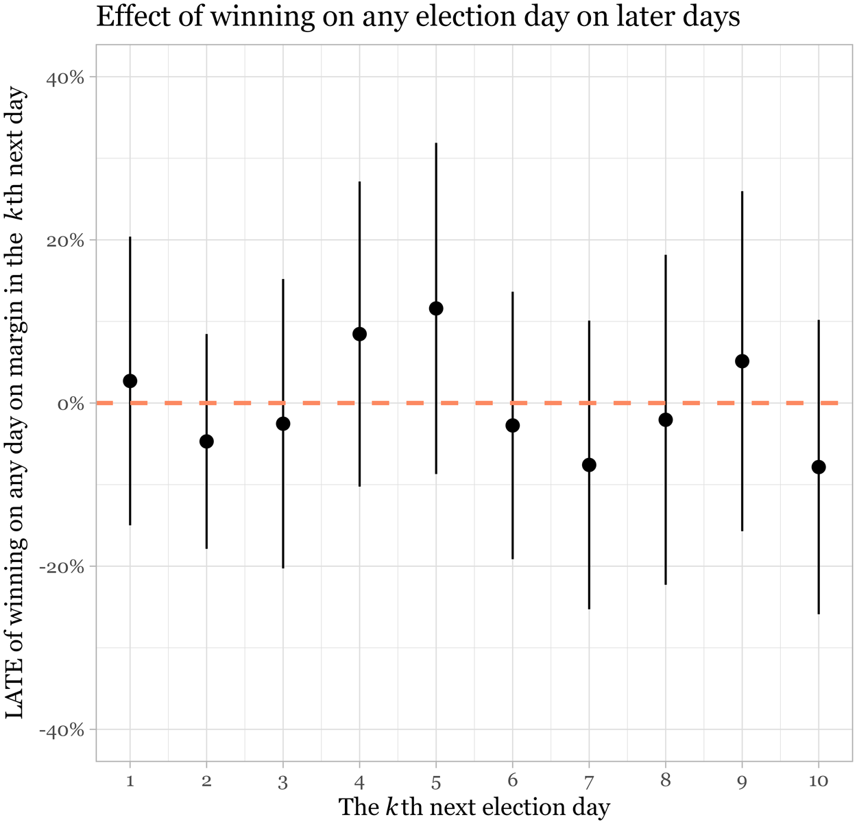
If early success is to yield success later on in the race through a sequence of momentum-driven wins, winning in election  $t$ should not only affect the next election, but part of these effects should also persist in the following elections. To see if this is the case, we replicate the long-term analysis implemented above, but this time using winning in any election $t$ as treatment. As shown in Figure 4, the effect of winning on any election day on later election days shows a consistent null result. It seems that in the case of the American primaries, we see no success-breeds-success pattern.
The effect of winning in any state on the margin in later election days.

4.3. Robustness and sensitivity analyses
To assess whether our results are driven by any specific race, we conduct a test where we drop each race one by one for each party and re-run our main models, as presented in Tables 2 (columns 1 through 4) and 3 (columns 1 through 3). Figure 5 reports the results of this test. The red line shows the original coefficients with all races included, equivalent to those reported in these two tables. Each black dot represents an iteration of the jackknife analysis, with each iteration dropping a specific race (shown on the  $y$-axis). The analysis thus allows us to compare whether dropping specific races makes the coefficients change as compared to a model with these observations included. The results indicate that, with one exception in facet (3) for the 1996 Rep, all the jackknife estimates are not statistically indistinguishably different from the reported main effects (the red line). In addition, all the results for any state on the next (facets 5) are not statistically different from 0 (the grey line). It thus seems unlikely that our results are driven by specific races. Further, Figure 5 highlights that the historical record gives us hardly any data, as there have not been very many primary elections since the reforms.
Jackknife test.

Further, in Table 4, we look at dropping out of the race as an alternative outcome. This measure is crucial, as dropping out captures the key mechanism through which candidates who fail to benefit from bandwagon effects ultimately underperform. Specifically, we create a variable for the proportion of the race candidates who participate in. For example, a value of 1 means that a candidate stays until the convention, while a value of 0.5 means that they drop out after half the number of election days. The mean of this variable is 0.63 and the SD is 0.33. The signs and significance of the coefficients using this outcome are in line with the main results presented in Table 2. One potential concern with these analyses is the presence of “symbolic” candidates who continue campaigning despite consistently poor performance for the sake of participating, generating media attention for other future races. To investigate if this is a problem, we follow suggestions by Coppock (Reference Coppock2019) on how to deal with non-response in audit experiments and find that results remain unchanged when we code missing outcomes as zero (in most cases because candidates drop out), as can be seen in Table 5.
Regression discontinuity results predicting the proportion of races a candidate participates in

Note: Models estimated using RDRobust (Calonico et al., Reference Calonico, Cattaneo and Titiunik2015). Dependent variable: the proportion of the primary a candidate participates in. The standard errors are clustered at the candidate level, and we use the “robust” SEs.  $^{*}\mathrm{p} \lt 0.05$; $^{**}\mathrm{p} \lt 0.01$.
Regression discontinuity results with missing outcomes coded as 0

Note: Models estimated using RDRobust (Calonico et al., Reference Calonico, Cattaneo and Titiunik2015). Dependent variables: victory margin on the Xth day on the margin in the next election day. The standard errors are clustered at the candidate level, and we use the “robust” SEs.  $^{*}\mathrm{p} \lt 0.05$; $^{**}\mathrm{p} \lt 0.01$.
In Section A.3 of the Online Appendix, we discuss a further set of robustness checks that test the sensitivity of our results to the use of specific modeling strategies as well as the inclusion of potentially problematic primaries. First and foremost, in Section A.4, we discuss two additional approaches to dealing with missing values—what we do with, for instance, candidates who drop-out of the race. First, whenever there are no results for a candidate (for instance, when they dropped out), their vote share can be filled forward based on their last recorded result. Second, we can simply use only non-missing information, thereby dropping candidates when they fail to participate in an election. Furthermore, in Section A.5, we present several alternative outcomes to show that the results do not depend on the outcome chosen nor on using the most important state on each election day as the next election. We focus on: the number of races a candidate wins, whether a candidate wins the nomination, the proportion of races on each election day won, and the mean winning margin of all races on each election day. Finally, in Section A.6, we test whether winning matters if candidates become the front runner after not being the number one in the election before, as well as the effect of coming in second and unexpectedly being the runner up. Our results are consistent across all these tests.
5. Discussion
We find no conclusive evidence that winning in the Iowa caucus influences later election results. To the extent that it does exercise some influence, this seems to be more negative than positive for the electoral prospects of the winner. Moreover, whilst winning in New Hampshire seems to be associated with success in the fourth next state, this advantage is sensitive to bandwidth selection and does not carry over to elections in later states. Overall, despite the majority of studies being in agreement and the disproportionate public attention given to the early states as the “fish bowl” stage (Adkins and Dowdle, Reference Adkins and Dowdle2001) of the primary elections, the relevance of winning here does not appear to exceed the small delegate numbers the winners add to their totals counted at the convention. True, primaries can operate as feeling thermometers, revealing the chances of candidates, without, however, translating this role into a momentum effect for winners.
The conclusion we reach is compatible with research on the “invisible primary”—the crucial role political elites play in determining who becomes a candidate in the first place. Research in this area argues that much of the nomination action takes place before voters attend a caucus or cast a ballot: the influence of the invisible primary outweighs the impact of early wins (e.g. Mayer, Reference Mayer2003; Cohen et al., Reference Cohen, Karol, Noel and Zaller2008). Our finding that victories in early contests are not as crucial as found in the two dozen previous empirical studies we reviewed is consistent with this body of literature.
When it comes to who wins in a primary race, our findings speak to concerns that the first races would undermine the fairness and representativeness of the election process by placing too much power in the hands of early voters from non-representative states (Winebrenner, Reference Winebrenner1983; Klumpp and Polborn, Reference Klumpp and Polborn2006). Our main result questions the practice of “frontloading,” whereby states compete in a Red Queen’s race to move their own primaries and caucuses to take place earlier and earlier in the campaign in order to retain influence on the eventual result (Mayer and Busch, Reference Mayer and Busch2003; Aldrich, Reference Aldrich2009; Kamarck, Reference Kamarck2009; Christenson and Smidt, Reference Christenson and Smidt2012). Finally, the absence of an overall bandwagon effect of winning, even when the analysis is performed on the pooled dataset, strengthens the null findings for just the first-in-the-nation states, as it suggests that the lack of a large significant effect is not simply due to a small- $n$ problem. This null also speaks more generally about the need to rethink how primaries work and what cumulative effects we should expect in the process.
We hasten to point out a key limitation to our study: our interpretation of the conventional wisdom about momentum. Winning and vote share are two different operationalizations of perfomance, as one can have a high vote share or win yet still perform worse than expectations. Here we have focused in particular on “winning” as the hypothesized driver of momentum. By focusing specifically on winning, our analysis does not speak to momentum effects created by a high vote share. However, focusing on vote share alone does not permit a strict causal test of the momentum effect, and because correlational evidence dominates this literature, causal evidence on winning remains an important contribution. That said, our results pertain solely to the “winning” operationalization of performance. While winning is a key variable in this literature, vote share is a more common independent variable and our results do not speak to analyses that employ it. For instance, while our analysis finds no evidence of an effect of coming in first, it may be that what matters is ending among the top candidates.
Our analysis has another key limitation, which it shares with previous studies, namely the inevitably limited number of data points: There simply have not been all that many races in Iowa and New Hampshire yet since the 1969 reforms. Whilst we wrangled all the statistical power we could from the data, the analysis leaves open the possibility of a positive effect that is small enough to escape statistical detection. Alternatively, it may be the case that there have only been a handful of elections where the early states matter (e.g. Obama in 2008 and Trump in 2016), and these effects are muted on average. Further, alongside these elections, there may be others where election night uncertainty about the results, for example, in Iowa in 2012 and 2020, may affect the actual measurement of who “won” the election, potentially muting or delaying momentum effects. Put differently, the fact that there have been few primaries since the 1976 reforms not only limits statistical power, but it also makes any effects more sensitive to particular cases. These limitations aside, we believe that our study helps in elucidating a problem that had remained hidden under the carpet of multivariate regression analyses in the past: there is simply not enough information yet available that would serve to compare just-winners with otherwise identical just-losers in Iowa and New Hampshire.
An additional possibility the present analysis leaves open is that it is not winning per se that matters but exceeding expectations (Aldrich, Reference Aldrich1980; Adkins and Dowdle, Reference Adkins and Dowdle2001; Redlawsk et al., Reference Redlawsk, Tolbert and Donovan2011). Indeed, Donovan et al. (Reference Donovan, Redlawsk and Tolbert2014) find that Santorum’s media coverage experienced a large jump in 2012 immediately after the surprising success he had in Iowa, despite being a close second in the initial delegate count and being declared winner not until more than two weeks later. However, while an effect of winning can be disentangled from baseline correlations across states through a regression discontinuity design, an equivalent design is not readily available for identifying a “doing better than expected” effect. In Section A.6 of the Online Appendix, we show results of an analysis of primary contests in which winning leads a runner-up to become a frontrunner, and to thus exceed expectations vis-a-vis earlier contests. No effect of exceeding expectations is found. However, this operationalization is imperfect. Exceeding expectations is not merely a matter of outperforming earlier results; it involves doing better than anticipated by political observers and the media. Without direct measures of these expectations, no definitive conclusions can be drawn. Developing such measures is a key task for future research.
These limitations notwithstanding, the results leave us with a puzzle. The theoretical mechanisms through which a win in one state would have positive spillover effects on performance in a later election are well-established. How then can winning in either Iowa or New Hampshire not matter much for securing the presidential nomination? A consideration of the entire sequence of state elections may provide an answer. Suppose there really is a modest effect and we simply do not have enough historical data to identify it, e.g. that a win on one election day does increase the victory margin on the next election day by, say, 5%. This will often still not be enough to turn a loss into a win on that next day. So if a win in state 1 increases the probability of a win in state 2 by less than one, then it must indirectly increase the probability of a win in state 3 by even less. Or, similarly, if a 10% increase in vote share in state 1 generates a 5% increase in vote share in state 2—which would be a substantial spillover effect—then it still only creates a 2.5% increase in vote share in state 3. It becomes clear then that unless spillovers are disproportionately sized, their effects wane and momentum is lost rather than gained. This self-correcting nature of social influence dynamics has been observed elsewhere (Elster, Reference Elster1989; Goeree et al., Reference Goeree, Palfrey, Rogers and McKelvey2007; Van de Rijt, Reference de Rijt2019). We conclude that any effect that we were not able to rule out because of statistical power would be modest and thus fizzle out quickly, failing to impact who is ultimately nominated for president of the United States, and therefore calling into question whether the first days are really of primary importance.
Supplementary material
The supplementary material for this article can be found at https://doi.org/10.1017/psrm.2026.10096. To obtain replication material for this article, please visit https://doi.org/10.7910/DVN/FYQWJK.


 Open access