





Introduction
Glaciers provide a year-round source of fresh water, released from melting glacial ice (Immerzeel and others, Reference Immerzeel2020). Dwindling water resources in shrinking glaciers therefore present a risk to the water security of populations in basins downstream of mountain glaciers (Immerzeel and others, Reference Immerzeel, van Beek and Bierkens2010). High Mountain Asia contains the greatest mass of glacial ice outside of the polar regions (Shean and others, Reference Shean, Bhushan, Montesano, Rounce, Arendt and Osmanoglu2020), and glacial meltwater is an important contributor to the flow of major rivers such as the Indus and Amu Darya (Armstrong and others, Reference Armstrong2019). Therefore, reliable projections of glacier mass balance in High Mountain Asia in response to climate change are crucial for improving freshwater management and hazard mitigation.
The surface mass balance of a glacier is determined by the competing processes of accumulation (mostly snowfall and avalanching) and ablation (mainly meltwater runoff and sublimation for terrestrially terminating glaciers). Annual accumulation is an important component of mass balance; Jouberton and others (Reference Jouberton2022) attribute over 50% of mass loss this century from a glacier in southeastern Tibet to changes in accumulation, resulting primarily from a shift from solid to liquid precipitation due to increasing air temperature. ‘Accumulation’ is here used consistently to encompass all processes which add mass to the glacier, even where that mass is subsequently removed during the same year via ablation (accumulation therefore does occur in the ablation area by this definition).
Accumulation due to snowfall depends on both the volume of precipitation that falls on the glacier and the proportion of this precipitation that is solid. Modelling snow accumulation at the glacier scale therefore requires both precipitation and solid precipitation ratio to be distributed over the glacier surface through parameterization. Meteorological factors such as precipitation, air temperature and humidity often respond strongly to changes in elevation (e.g., Pepin and others, Reference Pepin2022), so parameters used to distribute point meteorological data over a glacier surface based on elevation are needed to model accumulation. Temperature and precipitation gradients are employed by many glacier mass-balance models, as are one or more air-temperature thresholds for discriminating precipitation phase (e.g., Gurgiser and others, Reference Gurgiser, Mölg, Nicholson and Kaser2013).
Appropriate parameter values to distribute meteorological variables in High Mountain Asia vary both spatially and temporally (e.g., Guo and others, Reference Guo, Wang and Tian2016). Deriving appropriate parameter values from local observations is important for accurate modelling of glacier accumulation, but this is difficult in high-altitude regions due to the scarcity of observations (Matthews and others, Reference Matthews2020; Thornton and others, Reference Thornton, Pepin, Shahgedanova and Adler2022) and large uncertainties in modelled precipitation products (Mishra, Reference Mishra2015). The High Mountain region of the central Himalaya covers 24% of the area of Nepal, but only contains 7% of the country’s precipitation gauges, and 8% of its air-temperature sensors (Talchabhadel and Karki, Reference Talchabhadel and Karki2019). The few precipitation gauges that exist in this region are mostly located in valley bottoms, from which observations are then interpolated over large areas with complex heterogeneous topography. This process may lead to unrealistic estimates of precipitation when producing gridded precipitation products (Miao and others, Reference Miao, Immerzeel, Xu, Yang, Duan and Li2024), especially at higher altitudes where glaciers are located. Moreover, many of the precipitation gauges in the valley do not have wind shields and, as such, underestimate the rate of precipitation, particularly snow (Cauteruccio and others, Reference Cauteruccio, Chinchella and Lanza2024).
A survey of some of the globally applied glacier mass-balance models included in the Glacier Model Intercomparison Project (GlacierMIP) (Hock and others, Reference Hock2019) reveals a wide variety of values for temperature and precipitation gradients and precipitation-phase thresholds, summarized in Table 1. Some of these values are calibrated using local data, but many are invariant worldwide, with values representing global averages or derived from global-scale calibration. The meteorological observations used to derive these parameter values are not, however, evenly distributed across the world’s mountain glacier regions. High-altitude observatories are overwhelmingly concentrated in Europe; the density of precipitation gauges in High Mountain Asia is less than 1% of that recommended by the World Meteorological Organization (WMO) (Shahgedanova and others, Reference Shahgedanova2021). This observational bias raises the question of whether the parameters employed by global mass-balance models to model accumulation are appropriate for use in the central Himalaya.
Summary of precipitation phase, temperature gradient and precipitation gradient parameter values from a selection of GlacierMIP models. Values given are either global or, where regional, encompass the Khumbu Valley.

ST = solid precipitation threshold temperature, LT = liquid precipitation threshold temperature, TG = temperature gradient, PG = precipitation gradient. ‘ $Calibrated^L$’ signifies that the parameter value concerned is derived at a glacier scale using local data. ‘ $Calibrated^M$’ signifies that it is calibrated using mass change observations.
Even when parameter values are calibrated based on locally available data, these can be subject to over-fitting and equifinality, where multiple combinations of parameter values would fit the observations equally well (Zolles and others, Reference Zolles, Maussion, Galos, Gurgiser and Nicholson2019; Rounce and others, Reference Rounce, Hock and Shean2020), so the applied combination is somewhat arbitrary. This can lead to glacier mass-balance modelling, which produces appropriate outcomes for the wrong reasons (e.g., melt factors in empirical models that are unphysically high to compensate for inflated estimates of accumulation). Such models may not be robust to changes of the period or region modelled, particularly for longer-term glacier mass-balance modelling under climate change. Assessing derived parameter values through consideration of physical processes could therefore improve confidence in the transferability of parametrizations through space and time.
Evaluating and improving parameterizations of accumulation in high-altitude regions of the central Himalaya requires several steps. Firstly, observations from a high-altitude region need to be used to derive appropriate values for accumulation modelling parameters. Secondly, these values can be compared with those employed by worldwide glacier models, such as those of GlacierMIP, to assess the latter’s applicability to glaciers in the central Himalaya. Thirdly, the modelled accumulation is assessed for its sensitivity to changes in air temperature. Finally, the parameter values derived from observations need to be physically interpreted in order to assess their validity and the limits of their transferability over wider spatial and temporal domains.
The Khumbu Valley, Nepal, is a remarkably well-observed glacierized area in the central Himalaya. Several overlapping networks of weather stations have been installed over recent decades, including up to 8810 m, almost at the summit of Everest (Matthews and others, Reference Matthews2022). This region therefore provides an unprecedented opportunity to investigate the meteorological factors affecting glacier accumulation in the central Himalaya, and to place parameterizations used in global mass-balance modelling into a local context. Here, we specifically employ this exceptionally detailed observational record to evaluate seasonal temperature gradients, the precipitation gradient and optimal precipitation phase temperature thresholds. This analysis enables us to estimate Khumbu Glacier accumulation and, furthermore, to inform our understanding of physical processes. The latter enables us to test the extent to which parameterizations used within global-scale GlacierMIP models are suitable for modelling accumulation in the central Himalaya.
Study area
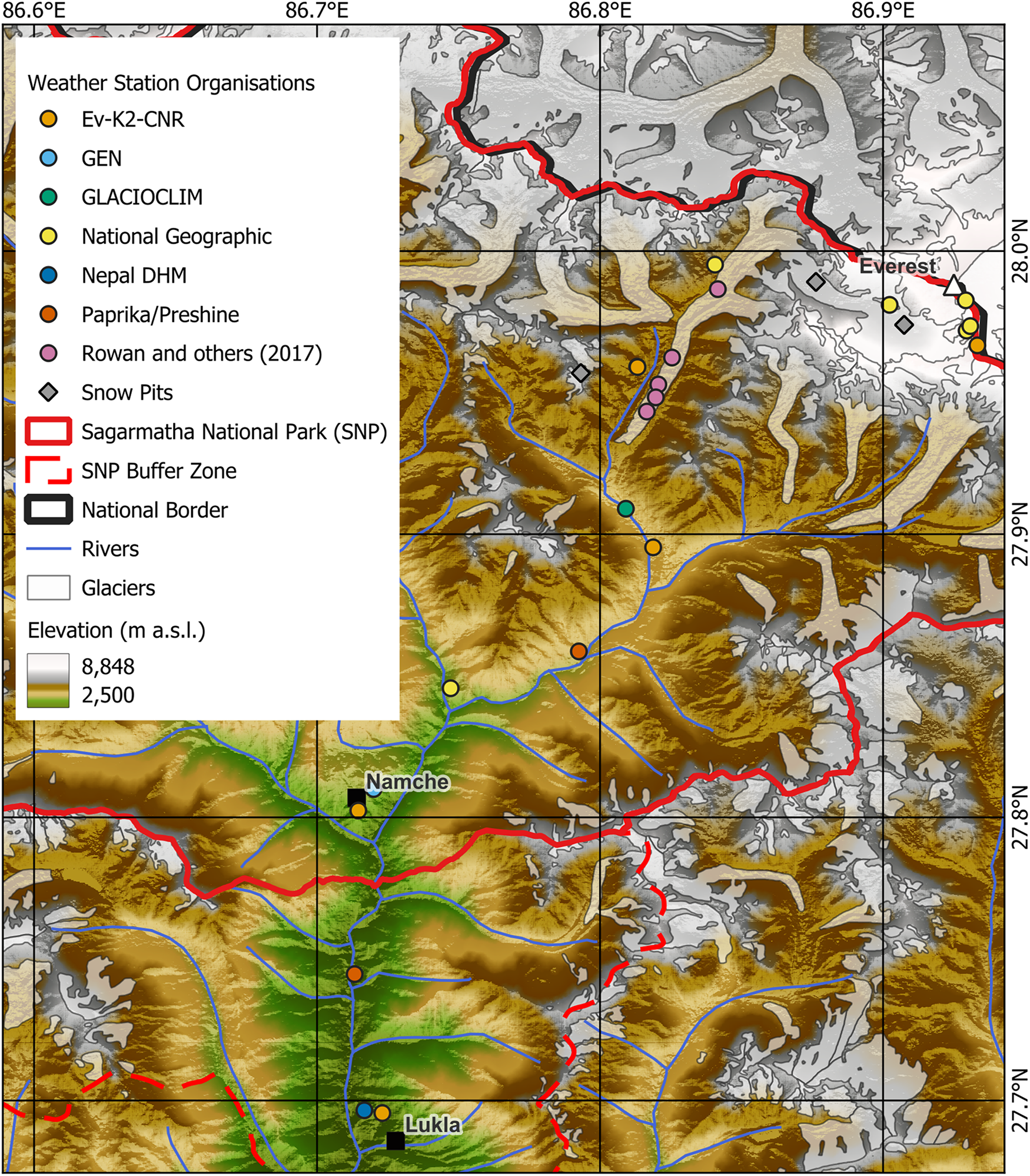
The Khumbu Valley is situated in Eastern Nepal, in the central Himalaya. It intersects with Sagarmatha National Park (SNP) and the SNP Buffer Zone, and extends up to the summit of Mount Everest at 8848.86 m above sea level (for a map, see Fig. 1). It constitutes part of the catchment of the Dudh Koshi river, which runs through the bottom of the valley, and is partially fed by meltwater from the numerous glaciers occupying the upper valley (Soncini and others, Reference Soncini2016). The Dudh Koshi is a tributary of the Koshi River, which is in turn the third-largest tributary to the Ganges. The annual cycle in the Khumbu region is divided into four seasons: pre-monsoon (March–May), monsoon (June–September), post-monsoon (October–November) and winter (December–February) (Hannah and others, Reference Hannah, Kansakar, Gerrard and Rees2005). Diurnal precipitation reaches a maximum during the night in the lower valley, and in early evening in the upper valley (Perry and others, Reference Perry2020).
Map of the Khumbu Valley, showing the locations of weather stations in Table 2. The Ev-K2-CNR and GLACIOCLIM stations at Pyramid (27.96°N, 86.81°E) are closely located and the GLACIOCLIM symbol is obscured. Elevation data is from a 30 m resolution ASTER-GDEM v3 digital elevation model. River, national border and SNP shapefiles are from the International Centre for Integrated Mountain Development (ICIMOD). Glacier shapefiles are from the Randolph Glacier Inventory (RGI) v.7 (RGI Consortium, 2023).

The Khumbu Glacier is located in the upper reaches of the Khumbu Valley on the southern slopes of Mt. Everest. It extends from a terminus elevation of 4879 m to a maximum elevation of 7981 m, with a median elevation of 6025 m (RGI Consortium, 2023). It is a summer-accumulation glacier (Sakai and others, Reference Sakai, Nuimura, Fujita, Takenaka, Nagai and Lamsal2015), as up to 76% of annual precipitation on the lower glacier falls during the monsoon (Perry and others, Reference Perry2020). The ablation area of the glacier is covered with a layer of rock debris, the thickness of which is highly heterogeneous (Rounce and others, Reference Rounce, King, McCarthy, Shean and Salerno2018). The accumulation area is above the Khumbu Icefall and begins at an elevation of around 5600 m.
Data and methods
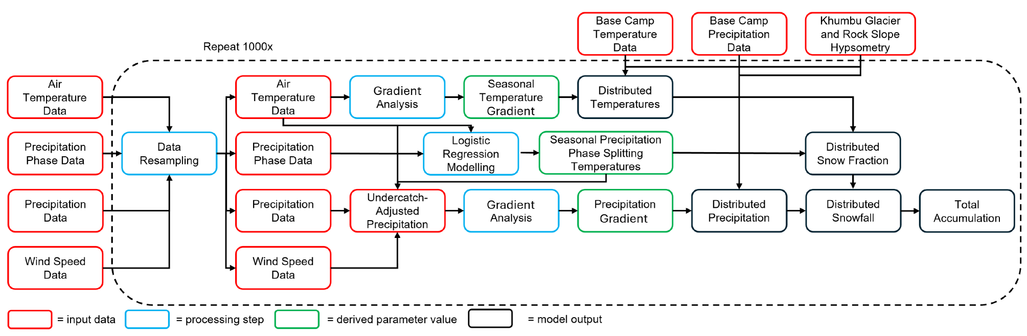
In situ meteorological data from the Khumbu Valley were used to assess precipitation phase threshold temperatures (the air temperatures at which precipitation changes phase, from solid to mixed or mixed to liquid), air temperature gradients and precipitation gradient. The appropriate values for these parameters derived from the observations were then used to model the accumulation over the surface of the Khumbu Glacier. The same accumulation modelling strategy was also used with the parameter values employed by GlacierMIP models (Table 1), in order to assess their suitability for modelling accumulation in this region of the central Himalaya. Uncertainty was assessed by repeating the analysis described in the following sections using a 1000-member bootstrap ensemble. This approach involves resampling the entire dataset of meteorological input data with replacement 1000 times and running the full modelling procedure each time, in order to gauge confidence intervals for the model results (Hesterberg, Reference Hesterberg2011). A schematic to summarize the methodological approach is provided in Fig. 2, and further details of the relevant steps are provided below.
Schematic of how accumulation is modelled using meteorological data. At the ‘Data Resampling’ step, all input meteorological data are randomly resampled (with replacement).

Meteorological data
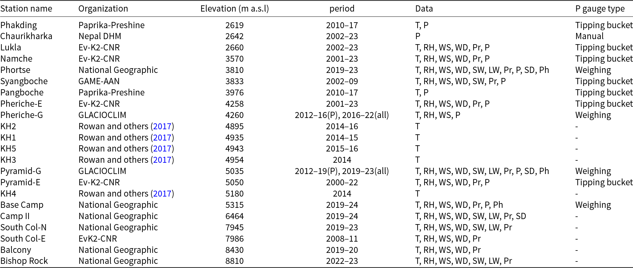
Meteorological data from 22 locations in the Khumbu Valley have contributed to this study. These include: co-located precipitation gauges and air-temperature sensors at Phakding and Pangboche, established by the Paprika-Preshine projects (Chevallier and others, Reference Chevallier2017), a rain gauge at Chaurikharka, established by the Department of Hydrology and Meteorology (DHM), Government of Nepal, weather stations at Lukla, Namche, Pheriche, Pyramid and the South Col, established by the Ev-K2-CNR organization (Salerno and others, Reference Salerno2025), a weather station at Syangboche, established by the Glaciological Expedition to Nepal (GEN) (Ueno and others, Reference Ueno1996), on-glacier air-temperature sensors established by Rowan and others (Reference Rowan, Quincey, Gibson and Irvine-Fynn2017), weather stations at Pheriche and Pyramid established by GLACIOCLIM and five weather stations ranging between Phortse and the Everest summit established by the National Geographic and Rolex Perpetual Planet Everest Expedition (Matthews and others, Reference Matthews2020, Reference Matthews2022). All the above sites are summarized in Table 2 and mapped in Fig. 1.
Station locations are mapped in Figure 1.

T = air temperature, RH = relative humidity, WS = wind speed, WD = wind direction, SW = shortwave radiation, LW = longwave radiation, P = precipitation, Pr = atmospheric pressure, SD = snow depth, Ph = precipitation phase.
Snow pit data
Previously unpublished snow pit data collected by the author team in three locations were also used as a comparison for modelled snowfall: Lobuche East (5900 m, collected May 2019), Camp 1 (5943 m, collected May 2024) and Camp 2 (6400 m, collected May 2019). At each location, snow water equivalent (SWE) was directly measured using a Snowmetrics snow density tube sampler and/or wedge sampler. The bottom of the annual layer was inferred by the presence of higher density and darker snow/firn. Total observed SWE of the annual layer is expected to be less than liquid equivalent precipitation as a result of some ablation due to sublimation and melt.
Precipitation phase modelling
Precipitation phase was modelled as a function of air temperature using logistic regression at sites where concurrent observations of both variables were available: Phortse (3810 m), Pyramid-G (5035 m) and Base Camp (5315 m), where automatic weather stations recording air temperature were co-located with disdrometers (which use lasers to sense precipitation phase). Phase data were collected by the disdrometers once every hour at Phortse and Base Camp, and once per minute at Pyramid-G. Data from these three sites were pooled and then filtered to only include observations when air temperatures were  $\geqslant$ –4 °C and $\leqslant$ 8 °C, the limits within which precipitation phase could not be anticipated (Liu and others, Reference Liu, Yan, Qin, Weng, Lu, Dong and Gong2018). The reasons for this are that a) observations of liquid precipitation at $ \lt $ –4 °C or solid precipitation at $ \gt $ 8 °C were likely to be due to instrument error, and b) assessments of the efficacy of the logistic regression modelling would be inflated if the model was being tested on a high proportion of ‘easy’ cases.
The logistic regression model was trained on a random 70% of the filtered data, and predicted the probable phase of the remaining 30% based on the corresponding air temperature data. The air temperatures at which the probability of precipitation being liquid predicted by the model was 10% (hereby ST) and 90% (hereby LT) were used to categorize observed precipitation as either solid (10% or lower probability liquid, i.e., T $\leqslant$ ST), liquid (90% or higher probability liquid, i.e., T $\geqslant$ LT), or mixed (between ST and LT exclusive). These thresholds were chosen to fit phase modelling closely to observations without including extreme and potentially erroneous values (Jennings and others, Reference Jennings, Winchell, Livneh and Molotch2018). Within the range of temperatures corresponding to mixed precipitation, the fraction of liquid precipitation was interpolated linearly. This enabled the total volume of solid precipitation to be modelled, including the solid fraction of the mixed precipitation. All logistic regression fitting and evaluation was assessed seasonally, with observations from the winter and post-monsoon seasons pooled due to a scarcity of liquid precipitation events, particularly in winter.
Temperature gradients
Seasonal temperature gradients throughout the Khumbu Valley were assessed using the air-temperature sensors listed in Table 2. Each location was only included where there was an uninterrupted season of data. For each station, the mean temperature for each season of available data was found (e.g., pre-monsoon 2016, monsoon 2016, etc.). The median value of the seasonal means (e.g., the median of the winter means across all years) at each location was then used in linear and quadratic regressions, which employ elevation as the predictor variable. The first derivatives of the linear expressions are the gradient; they vary with altitude for the quadratic functions.
Throughout this study, the term ‘temperature gradient’ refers to the near surface change in air temperature with ascending elevation. Instances of the term ‘lapse rate’ in this study instead refer to the reduction in temperature with altitude in the free atmosphere.
Precipitation gradient
The annual precipitation gradient over the elevation range of the Khumbu Valley was investigated using data from several networks of precipitation gauges. Recorded precipitation was adjusted for wind-induced undercatch using several transfer functions which depended on the precipitation phase (as modelled using air temperature as described above) and the precipitation gauge shield configuration. The functions developed by Kochendorfer and others (Reference Kochendorfer2017) were used for solid and mixed-phase precipitation from unshielded and single-shielded gauges; the functions developed by Kochendorfer and others (Reference Kochendorfer2018) were used for solid and mixed precipitation from double-shielded gauges; and the functions developed by Masuda and others (Reference Masuda, Yatagai, Kamiguchi and Tanaka2019) were used for liquid precipitation from unshielded and single-shielded gauges. Liquid precipitation at sites with double shields was left unadjusted because there are no suitable transfer functions for this combination.
Following the analysis in Salerno and others (Reference Salerno2015), an exponential decay function was fitted to the precipitation–elevation data. Thus the precipitation gradient was described in the form
 \begin{equation}
P(z) = x_1 \cdot e^{-x_2 \cdot z}+x_3
\end{equation}
\begin{equation}
P(z) = x_1 \cdot e^{-x_2 \cdot z}+x_3
\end{equation}where  $x_1$, $x_2$ and $x_3$ were coefficients determined by the curve fitting.
For comparison with the precipitation gauge data, monsoon precipitable water was modelled with respect to elevation. Air temperatures were distributed through the valley at a 500 m elevational resolution using the mean monsoon temperature at Phakding and the monsoon temperature gradient (as determined from the temperature gradient analysis). A vertical pressure profile was generated for the atmosphere at each surface altitude using the hypsometric equation. Then, a vertical temperature profile was generated for the atmosphere at each surface altitude, assuming a dry adiabatic lapse rate for the first 50 m above the ground, then a moist adiabatic lapse rate above that (based on an assumption that the atmosphere is saturated from 50 m above ground level during the monsoon). Lastly, the vertical profiles of temperature and pressure at each surface altitude were then used to calculate the precipitable water in each vertical column, and an exponential decay function was fitted to the modelled precipitable water and surface elevation relationship. The maximum height used for modelling the water column was up to a pressure level of 300 hPa, which is significantly above the elevation of the Everest summit (approximately 330 hPa). This precipitable water modelling was performed using the MetPy package (May and others, Reference May2022), in particular the ‘dry_lapse’, ‘moist_lapse’ and ‘precipitable_water’ functions.
This study does not apply a precipitation correction factor, as many mass balance models do (Hanus and others, Reference Hanus, Schuster, Burek, Maussion, Wada and Viviroli2024). This is because many of the processes for which a precipitation correction factor would be required, such as snow redistribution and undercatch, were accounted for in other ways in this accumulation modelling strategy.
Accumulation due to snowfall
The glacier-wide annual accumulation due to snowfall was modelled at a 50 m elevational resolution using the following equation:
 \begin{equation}
a_{snow} = \frac{\int_{z_{min}}^{z_{max}}\int_{t_{0}}^{t}f(z,t) \cdot P(z,t) \cdot A(z) \,dt \,dz} {\int_{z_{min}}^{z_{max}}A(z)\,dz}
\end{equation}
\begin{equation}
a_{snow} = \frac{\int_{z_{min}}^{z_{max}}\int_{t_{0}}^{t}f(z,t) \cdot P(z,t) \cdot A(z) \,dt \,dz} {\int_{z_{min}}^{z_{max}}A(z)\,dz}
\end{equation}where  $a_{snow}$ is snowfall accumulation in mm water equivalent (w.e.), t is time at hourly resolution ( $t_0$ being start of modelled period), z is the altitude of the lower bound of the given 50 m altitudinal band ( $z_{min}$ being terminus elevation and $z_{max}$ the maximum glacier elevation), f is the fraction of precipitation which is solid (between 0 and 1), P is precipitation within the given 50 m altitudinal band and A is the area of the given altitudinal band, derived from a 30 m resolution ASTER-GDEM v3 digital elevation model. The term f(z,t) is given by:
 \begin{equation}
f(z,t) = \left \{\begin{array}{rcl} 0 & for & T(z,t) \geqslant LT(t)
\\ 1 & for & T(z,t) \leqslant ST(t)
\\1-(\frac{T(z,t) -ST(t)}{LT(t)-ST(t)}) & for & ST(t) \lt T(z,t) \lt LT(t)
\end{array} \right.
\end{equation}
\begin{equation}
f(z,t) = \left \{\begin{array}{rcl} 0 & for & T(z,t) \geqslant LT(t)
\\ 1 & for & T(z,t) \leqslant ST(t)
\\1-(\frac{T(z,t) -ST(t)}{LT(t)-ST(t)}) & for & ST(t) \lt T(z,t) \lt LT(t)
\end{array} \right.
\end{equation}Here, LT and ST both vary by season, as described above, hence they are functions of t. Equation (3) linearly interpolates f between these precipitation phase threshold temperatures.
 \begin{equation}
T(z,t) = T_{BC}(t)+G(t) \cdot (z-5300)
\end{equation}
\begin{equation}
T(z,t) = T_{BC}(t)+G(t) \cdot (z-5300)
\end{equation}  $T_{BC}$ refers to the air temperature recorded at the Base Camp station, and G is the linear temperature gradient, which varies by season, as described above. G is negative. The 5300 in the brackets refers to 5300 m, the lower bound of the altitudinal interval within which the Base Camp station is located.
 \begin{equation}
P(z,t) = \frac{x_1 \cdot e^{-x_2 \cdot z}+x_3}{x_1 \cdot e^{-x_2 \cdot 5300}+x_3} \cdot P_{BC}(t)
\end{equation}
\begin{equation}
P(z,t) = \frac{x_1 \cdot e^{-x_2 \cdot z}+x_3}{x_1 \cdot e^{-x_2 \cdot 5300}+x_3} \cdot P_{BC}(t)
\end{equation}  $P_{BC}$ is the precipitation recorded at the Base Camp station. $x_1$, $x_2$ and $x_3$ are the coefficients of the exponentially decaying precipitation gradient as in Eqn (1). In Eqn (5), Base Camp precipitation is multiplied by the ratio between the values of the precipitation decay curve at a given altitude and that at Base Camp.
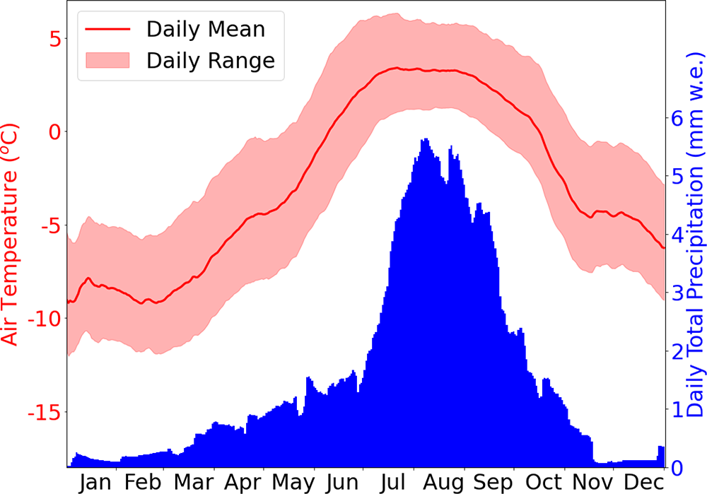
Year-long time series for  $T_{BC}$ and $P_{BC}$ were created by finding the mean recorded value of temperature and precipitation at each hour of the year since the Base Camp station has been operational (Fig. 3). This was done to preserve the seasonal and diurnal cycles of temperature and precipitation, while modelling an ‘average’ year.
The ‘average’ year at Base Camp used for the accumulation modelling. The daily mean temperature and daily total precipitation plotted are 31 day rolling means. The daily temperature range is produced by 31 day rolling means of daily minimum and maximum temperatures. This ‘average’ year was produced from the mean temperature and precipitation for each hour of the year recorded by the Base Camp station, from 4 years of data.

Redistributed snow contribution
The accumulation area of the Khumbu Glacier is surrounded by steep rock faces exposed to high winds, and avalanches onto the Khumbu Glacier surface are a common occurrence (Adhikari and others, Reference Adhikari, Dawadi and Nepal2023; Kneib and others, Reference Kneib2024). Therefore, estimates of accumulation must make some attempt to quantify the contribution from redistributed snow.
Many glacier mass balance models calibrate parameter values using observed mass changes (including JULES and Marzeion and others, Reference Marzeion, Jarosch and Hofer2012 from the GlacierMIP project). In these cases, mass balance is inferred from mass changes, so all processes of accumulation and ablation influence the calibration of parameter values, including redistributed snow. The calibrated precipitation gradient will therefore apply to the effective precipitation, which in this context refers to the total snow accumulation on the glacier surface, including that from redistributed snow.
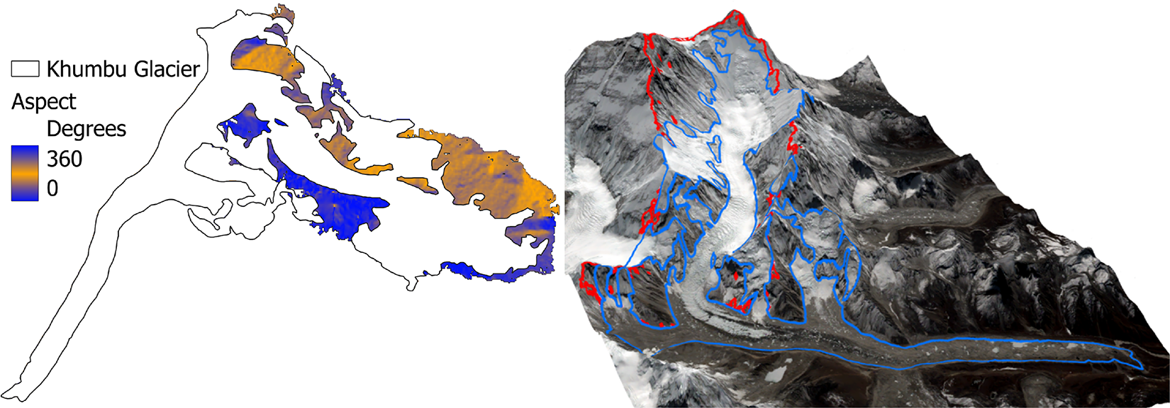
We calculate an approximate upper bound on the redistributed snow contribution by assuming that all solid precipitation which falls on surrounding slopes (distributed over this terrain using Eqn (2)) will at some point be redistributed onto the glacier. These surrounding slopes were identified by manually selecting surrounding rock faces which slope towards the glacier surface (highlighted in Fig. 4) using the aspect derived from the ASTER DEM (almost the entire area has a slope over 30°). An estimate of the effective precipitation was therefore provided by including the rock face area in the numerator of Eqn (2):
 \begin{equation}
a_{snow+rs} = \frac{\int_{z_{min}}^{z_{max}}\int_{t_{0}}^{t}f(z,t) \cdot P(z,t) \cdot A'(z)\,dt\,dz}{\int_{z_{min}}^{z_{max}}A(z)\,dz}
\end{equation}
\begin{equation}
a_{snow+rs} = \frac{\int_{z_{min}}^{z_{max}}\int_{t_{0}}^{t}f(z,t) \cdot P(z,t) \cdot A'(z)\,dt\,dz}{\int_{z_{min}}^{z_{max}}A(z)\,dz}
\end{equation}where  $A'$ refers to the combined area of the glacier and surrounding slopes within the given altitudinal band. The denominator is still the integral of A because the overall snow volume is divided by the glacier area only to produce glacier-wide accumulation in mm w.e.
Left: Map of glacier-surrounding rock face aspect for identification of redistributed snow contribution area. Right: RGI v.7 Khumbu Glacier extent is outlined on the 3D model in blue, with snow-contributing rock faces outlined in red. Note that the map and the 3D model do not have the same orientation.

This approach is limited in that it does not account for temporal variation in the rate of snow redistribution, which given the stochastic nature of avalanching will be considerable. It considers only a long-term average, on the principle that the snow deposited on surrounding rock faces will eventually be moved onto the glacier surface. In addition, snow blowing from further afield (outside the identified sloping rock faces) is not accounted for. This approach also does not account for sublimation of snow from surrounding rock faces, which may be substantial during the winter (Wagnon and others, Reference Wagnon2013), and is therefore likely an overestimate.
GlacierMIP models comparison
The above accumulation modelling strategy was also performed using the parameter values from models in GlacierMIP, as summarized in Table 1. Where values are ‘calibrated’, the locally appropriate parameter value as determined by this study was used. Note that this is not a case of using these models themselves to model accumulation but only using their parameter values within the accumulation modelling strategy described above (though these models employ fundamentally similar methods for modelling accumulation). For the models that calibrate parameter values using observed mass changes (JULES and Marzeion and others, Reference Marzeion, Jarosch and Hofer2012), snow redistribution is already accounted for when calibrating the parameter values. The accumulation modelled using these models’ parameter values was therefore found using Eqn (2), rather than Eqn (6). For all the other models, the gradients presented were interpreted as representing the non-effective precipitation, which does not account for snow redistribution, as opposed to the effective precipitation, which does.
Temperature sensitivity
To investigate the temperature sensitivity of the modelled accumulation, the input meteorological data from the Base Camp station were varied. Hourly temperature data were changed in increments of 0.5°C up to a maximum change of  $\pm$3°C, and the effect this had on annual glacier accumulation (inclusive of redistributed snow) was modelled. The temperature sensitivity of accumulation using the GlacierMIP models’ parameter values was assessed in the same way. Temperature sensitivity was quantified in two ways: firstly as an absolute value given in mm w.e. °C $^{-1}$, found from:
 \begin{equation}
\frac{a_{snow+rs}(T+1 ^\circ C)-a_{snow+rs}(T-1 ^\circ C)}{2}
\end{equation}
\begin{equation}
\frac{a_{snow+rs}(T+1 ^\circ C)-a_{snow+rs}(T-1 ^\circ C)}{2}
\end{equation}and secondly by returning the accumulation at each temperature change as a % of the modelled ‘no-change’ (i.e., T+0 °C) accumulation. Model sensitivity to precipitation was not investigated because the % change in accumulation would be exactly equal to the % change in precipitation, regardless of the model parameter values, as determined by Eqn (6).
Results
Precipitation phase modelling
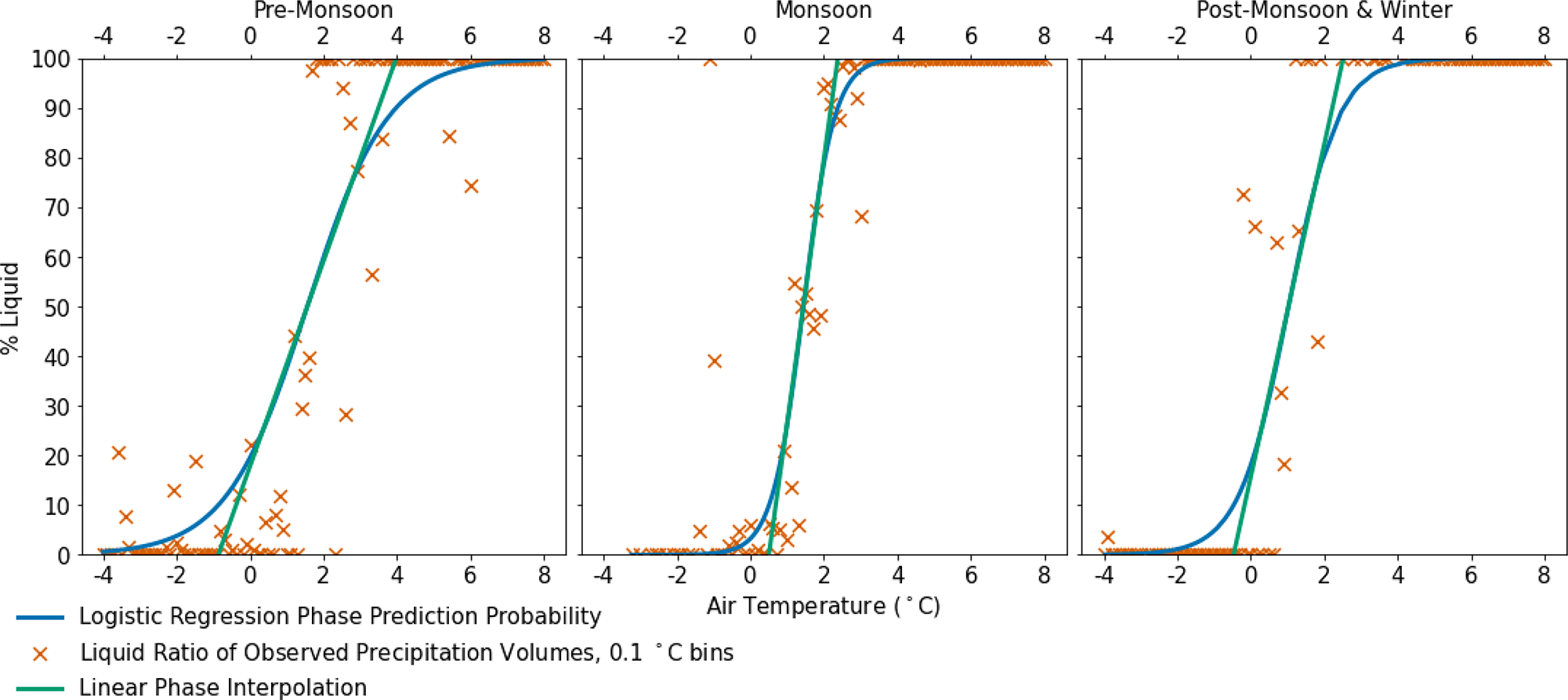
When transitioning from the pre-monsoon to the monsoon season, the solid precipitation threshold temperature increases from  $-0.96\pm0.71^\circ$C to $0.23\pm0.29^\circ$C, and the liquid precipitation threshold temperature decreases from $3.85\pm0.64^\circ$C to $2.17\pm0.20^\circ$C, reducing the temperature range of mixed-phase precipitation during the monsoon. This trend is to some extent reversed again when transitioning from the monsoon to post-monsoon and winter seasons, though the post-monsoon and winter values are closer to the monsoon than to the pre-monsoon values (Table 3). Due to the small number of observations, the post-monsoon and winter values have large uncertainties, which overlap with the monsoon values, and also with the pre-monsoon value in the case of ST, but the differences between the seasonal values are statistically significant (defined here and throughout this study as an ANOVA test p-value $ \lt $0.05) for both ST and LT. The predicted probability of liquid precipitation from the logistic regression model matches well with the proportion of liquid precipitation in each 0.1°C temperature bin as indicated by the disdrometer and precipitation gauge observations (Fig. 5).
Logistic regression modelling of precipitation phase by season, as described in the Data and Methods subsection precipitation phase modelling.

Seasonal precipitation phase thresholds as indicated by logistic regression modelling. Uncertainty ranges are estimated from the bootstrap resampling.

Temperature gradients
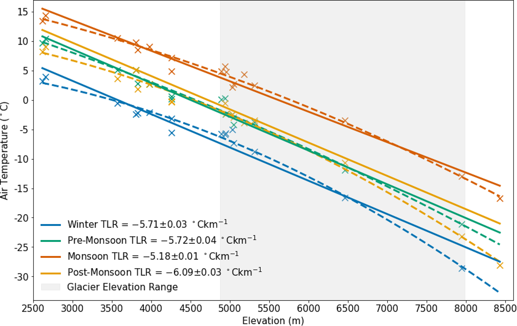
Near-surface temperature gradients calculated from station observations are least negative during the monsoon. For the seasonal gradients, using quadratic rather than linear functions provides a closer fit to the data (the difference is statistically significant, as found using a p $ \lt $0.05 ANOVA test), as gradients are more negative at higher elevations. This effect is reduced during the monsoon, and strongest in winter. The interpretation and applicability of the quadratic gradients are discussed more thoroughly in the Supplementary Material.
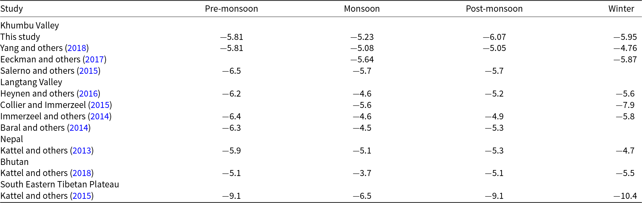
If linear fits are instead applied to the seasonal data (for comparison with previous studies), the temperature gradients obtained are  $-5.81\pm0.04^\circ$C km $^{-1}$ for the pre-monsoon, $-5.23\pm0.01^\circ$C km $^{-1}$ for the monsoon, $-6.07\pm0.03^\circ$C km $^{-1}$ for the post-monsoon and $-5.95\pm0.03^\circ$C km $^{-1}$ for winter (Fig. 6). These differences between seasonal gradients are statistically significant (found using a p $ \lt $0.05 ANOVA test), and demonstrate why an annual value of temperature gradient should not be used for modelling strongly seasonal phenomena such as glacier accumulation in this region. The uncertainty ranges on the linear temperature gradients are estimated from the bootstrap resampling.
Given that the monsoon is when the majority of snow accumulation happens, the monsoon temperature gradient is particularly salient for accumulation modelling. It is consistently the least negative of the seasonal gradients and has low interannual variability with a coefficient of variation of 3.5%. A more comprehensive analysis of the interannual variability of the seasonal temperature gradients is provided in the Supplementary Material.
Seasonal and annual temperature gradients found using temperature data from 19 locations in the Khumbu Valley. Stated gradients are linear (solid lines), though quadratic functions (dashed lines) give a closer fit to the data, particularly in winter.

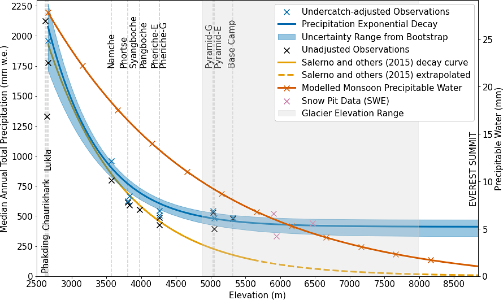
Precipitation gradient in the Khumbu Valley. The Salerno and others (Reference Salerno2015) gradient is included and extrapolated for comparison (that study did not extrapolate above 5600 m). Modelled monsoon precipitable water is also plotted (red line). The decay curve (blue line) is fitted only to the undercatch-adjusted gauge observations (blue crosses). The highlighted blue area corresponds to the uncertainty in the precipitation decay curve as estimated from the bootstrap resampling.

Precipitation gradient
Consistent with previous studies (Salerno and others, Reference Salerno2015; Karki and others, Reference Karki, ul Hasson, Gerlitz, Schickhoff, Scholten and Böhner2017), annual undercatch-adjusted precipitation can be modelled as a function of elevation with an exponential decay curve. However, the fitted coefficients of the decay curve found in this study (Eqn (8)) diverge from previous work in the region (Salerno and others, Reference Salerno2015):
 \begin{equation}
P(z) = 58800e^{-1.34\times10^{-3} \cdot z}+411
\end{equation}
\begin{equation}
P(z) = 58800e^{-1.34\times10^{-3} \cdot z}+411
\end{equation}Our revised precipitation function makes a considerable difference to modelled snow accumulation, particularly above 3500 m. A steep initial decrease in precipitation between 2500 and 4000 m begins to level out before reaching the elevation of the Khumbu Glacier terminus, and above 6000 m, modelled precipitation is approximately constant. Modelled precipitable water also follows an exponential decay with respect to elevation, demonstrating the importance of a dwindling moisture column as a control on precipitation (the decrease in precipitable water will also be a function of decreasing atmospheric column thickness). Annual accumulation estimates from the higher-altitude snow pits also fit closely to the values predicted by the precipitation exponential decay curve, providing some confidence that these findings continue to describe accumulation at least some extent into the accumulation area (though the snow pit data provides only a lower bound of accumulation, as the ablation rate is unknown). Annual point mass balances collected by GLACIOCLIM at 6350 m on the nearby Mera Glacier have an average value of 590 mm w.e., which also agrees closely with the Khumbu snow pit data and precipitation–elevation exponential decay curve. Interannual variability of the precipitation gradient could not be analysed as high-quality precipitation data across the elevational range of the valley was not available over multiple years.
Accumulation due to snowfall
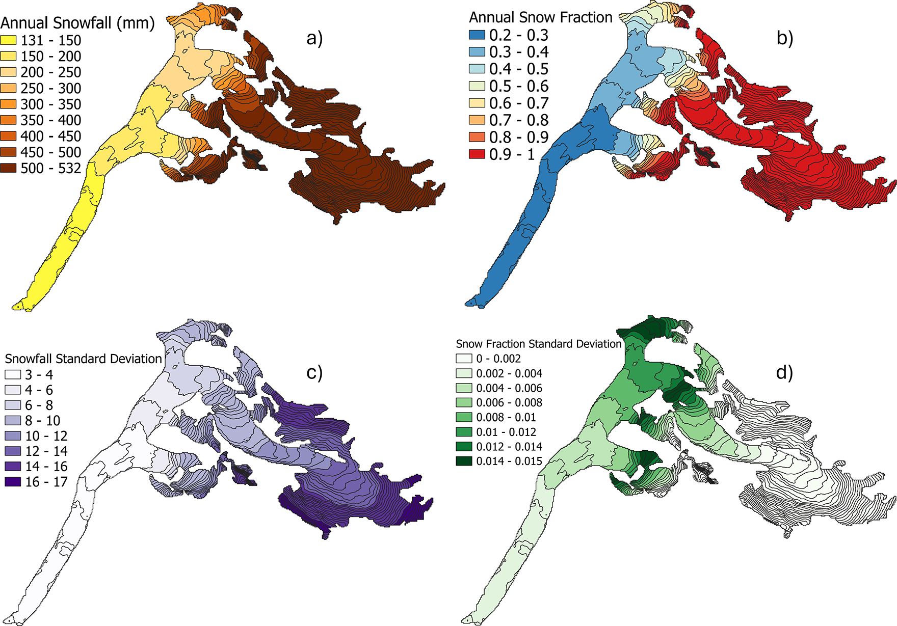
The glacier-wide annual accumulation due to direct snowfall is estimated at  $387\pm15$ mm w.e. Accumulation increases with altitude over the ablation area of the glacier from a minimum value of $131\pm3$ mm w.e. at the terminus to a maximum value of $532\pm12$ mm w.e. reached at 6400–6450 m. This altitudinal increase is due to an increase in the fraction of annual precipitation falling as snow, which is less than 0.5 up to 5400 m (this includes the entire ablation area, Fig. 8b). The peak accumulation value is reached when all the annual precipitation falls as snow, and this maximum value then remains almost constant over the accumulation area, due to the very shallow precipitation gradient (Fig. 8a).
Mapping of accumulation from direct snowfall (not accounting for redistributed snow) over the Khumbu Glacier by 50 m altitudinal bands: (a) annual snowfall (water equivalent), (b) snowfall as a fraction of annual precipitation, (c) standard deviation of annual snowfall and (d) standard deviation of snow fractions. The standard deviations were estimated using the bootstrap resampling.

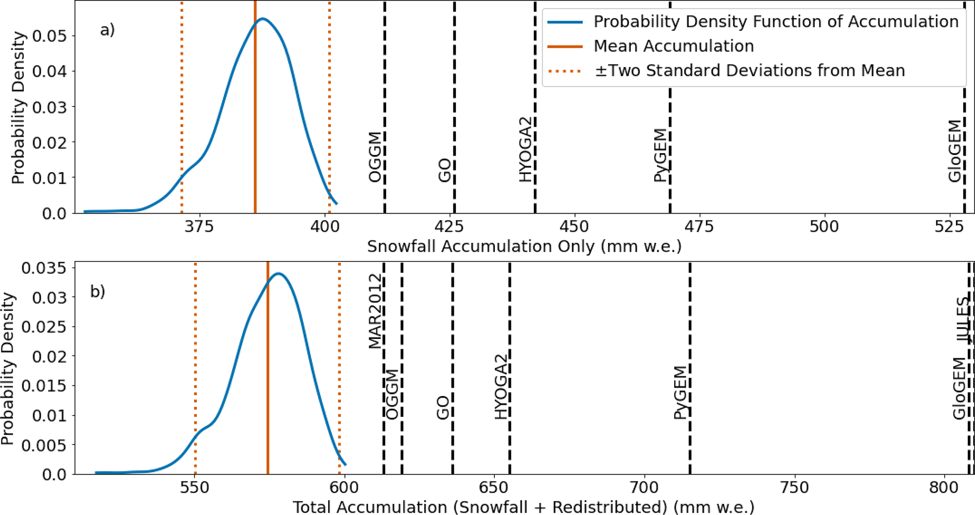
Parameter values taken from the GlacierMIP models result in substantially higher values of glacier-wide snow accumulation (Fig. 9a) that are even outside the range of the bootstrap resampling results produced in this study. The OGGM model gives the lowest estimate of glacier-wide accumulation among the GlacierMIP models (412 mm w.e.), while the highest estimate comes from GloGEM (528 mm w.e.). This suggests that the temperature and precipitation parameterizations embedded in the GlacierMIP models overestimate snow accumulation relative to approaches informed by local meteorological data.
Modelled accumulation using parameter values derived in this study (solid orange lines) as compared with those from GlacierMIP models (black dashed lines). The probability density function is produced using the bootstrap resampling.

Redistributed snow contribution
Based on the approach taken in this study, redistributed snow adds an additional 188 $\pm$9 mm w.e. to the glacier-wide snow accumulation, giving a total of 575 $\pm$24 mm w.e. Redistributed snow therefore represents 33% of the total glacier-wide accumulation.
When snow redistribution is estimated with the GlacierMIP model parameters, total snow accumulations are again higher than the values derived in this study, and outside the results of the bootstrap procedure (Fig. 9b). Similar to the snowfall-only modelled accumulation, the analysis suggests that these parameter values produce overestimations of Khumbu Glacier accumulation. In this case, the lowest total accumulation among these model parameter sets is Marzeion and others (Reference Marzeion, Jarosch and Hofer2012) at 613 mm w.e., and the highest is JULES at 810 mm w.e.
Accumulation sensitivity to temperature
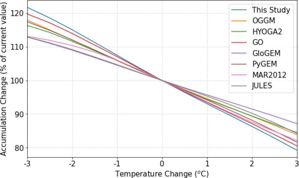
Results from the sensitivity analysis suggest that Khumbu Glacier snow accumulation has a temperature sensitivity of –41.7 mm w.e. °C $^{-1}$. Changing the input temperature data by $\pm3$ °C produced changes in modelled accumulation of a little over $\mp20\%$ (Fig. 10).
Temperature sensitivity of modelled accumulation using parameter values derived in this study (blue line), and using parameter values from GlacierMIP models. The slope of each line indicates the relative temperature sensitivity, as a % change in accumulation °C $^{-1}$.

Modelled accumulation using parameter values from the GlacierMIP models shows similar sensitivities to this in absolute terms, with the least sensitive being OGGM at –34.8 mm w.e. °C $^{-1}$ and the most sensitive being PyGEM at –43.0 mm w.e. °C $^{-1}$. However, given that the models themselves produce different total modelled accumulation, the most meaningful way to compare their sensitivities is by the percent change in modelled accumulation brought about by changes in temperature (Fig. 10). By this measure, all the GlacierMIP model parameter combinations exhibit lower sensitivity to changes in temperature than the accumulation modelled using the parameter values derived in this study. For instance, while the accumulation modelled using the parameterization in this study exhibits a 21% decrease under 3 °C of warming, using the GloGEM parameter values (the least sensitive) results in only a 13% decrease under the same circumstances. To summarize, using prescribed model parameter values rather than deriving them from in situ data produces modelled accumulation that is less sensitive to changes in temperature.
Discussion
Precipitation phase threshold temperatures show a statistically significant seasonal variation. In the transition from the pre-monsoon to the monsoon season, the value of LT decreases. This is consistent with the increased humidity, which reduces the difference between hydrometeor temperature and air temperature (Harder and Pomeroy, Reference Harder and Pomeroy2013), from which it follows that air temperatures closer to 0°C are required for solid precipitation. The temperature thresholds delineating the boundaries of mixed-phase precipitation narrow during the monsoon, which is also consistent with previous results showing a narrowing of the mixed-phase boundaries with increasing humidity (Jennings and others, Reference Jennings, Winchell, Livneh and Molotch2018). These trends are to some extent reversed in the transition from the monsoon to the post-monsoon and winter, when humidity falls again.
The use of quadratic seasonal temperature gradients, rather than linear, agrees with previous studies that found more negative temperature gradients at higher elevations (Khadka and others, Reference Khadka2021; Xu and others, Reference Xu, Xie and Zhu2022; Ghimire and others, Reference Ghimire, Singh, Khadka, Dawadi and Shrestha2023), but this effect is more pronounced outside the monsoon (Karki and others, Reference Karki, Hasson, Schickhoff, Scholten, Böhner and Gerlitz2020). In contrast, Yang and others (Reference Yang, Guyennon, Ouyang, Tian, Tartari and Salerno2018) found less negative gradients at higher elevations for all seasons except the monsoon. This discrepancy may result from the altitudinal range of the data; this study, Khadka and others (Reference Khadka2021); Xu and others (Reference Xu, Xie and Zhu2022) and Ghimire and others (Reference Ghimire, Singh, Khadka, Dawadi and Shrestha2023) all use data from above 8000 m, whereas Yang and others (Reference Yang, Guyennon, Ouyang, Tian, Tartari and Salerno2018) do not include data from higher than 5600 m.
The linear values of temperature gradients found here show a mixed degree of agreement with previous studies (Table 4). For the pre-monsoon and monsoon, results from this study agree with Yang and others (Reference Yang, Guyennon, Ouyang, Tian, Tartari and Salerno2018), who identified less negative temperature gradients than previous studies (Salerno and others, Reference Salerno2015; Eeckman and others, Reference Eeckman2017). This study finds a significantly more negative post-monsoon gradient than previous studies. The winter value found here agrees closely with that of Eeckman and others (Reference Eeckman2017), but finds a more negative gradient than that found by Yang and others (Reference Yang, Guyennon, Ouyang, Tian, Tartari and Salerno2018). As the majority of the annual precipitation falls during the monsoon, accurate estimates of temperature gradients during the monsoon are critically important for estimating glacier-wide snow accumulation.
Comparison of linear seasonal temperature gradients (°C km $^{-1}$) from this and previous studies.

The less negative temperature gradient during the monsoon season is consistent with a transition from a dry to a moist adiabatic regime (Khadka and others, Reference Khadka2021). Moist air masses moving up the valley release latent heat as water condenses, thereby warming the air at high elevations (Shea and others, Reference Shea, Immerzeel, Wagnon, Vincent and Bajracharya2015b). This has been observed at other locations in the central Himalaya (Kattel and others, Reference Kattel, Yao, Yang, Tian, Yang and Joswiak2013; Yadav and others, Reference Yadav, Pratap, Gupta, Dobhal, Yadav and Tiwari2019) and is unsurprising given the high relative humidity observed at all stations in the Khumbu Valley during the monsoon season (Xu and others, Reference Xu, Xie and Zhu2022).
For each of the seasonal temperature-elevation plots (Fig. 6), the quadratic relationships indicate less negative temperature gradients at low elevations and more negative gradients at high elevations. A physical interpretation for this is that the temperature gradient is closer to that of a moist adiabatic lapse rate at low elevations, where relative humidity is higher. As moisture condenses out of the air with increasing elevation, the relative humidity decreases, and the temperature gradient tends closer to that of a (more negative) dry adiabatic lapse rate; hence, the temperature gradient is non-linear. This is most pronounced in the post-monsoon and winter, when conditions are driest at high elevations. In the pre-monsoon and monsoon, humidity is high enough that the air remains close to saturation even at high altitudes, so the temperature gradient at high elevations does not tend towards a dry adiabatic lapse rate, and the temperature gradient across the valley elevational range remains close to linear. A more in-depth discussion of the interpretation and applicability of the quadratic temperature gradients, as well as their comparison with free-atmosphere lapse rates, is included in the Supplementary Material.
Further complicating this picture is the local situation of the temperature sensors. The lowest elevation temperature sensor included in this study, at Phakding, is located in the bottom of a steep cross-section of the valley, adjacent to the Dudh Koshi river. Local cooling, through topographic shading, cold air drainage, and the river itself may explain may explain the consistently lower temperatures recorded at Phakding than would be predicted from higher stations assuming a linear gradient (Fig. 6). The highest elevation temperature sensors used in the gradient analysis, at the South Col and Balcony, are in extremely windy locations and the radiation shields here may therefore be better ventilated than others, again leading to lower temperatures at the highest elevations and increasing the non-linearity of the gradients. In addition, the temperature sensors are mounted at a range of heights above the surface (between 1 and 2 m), which will affect the strength of the observed signal from solar heating of the surface. Given the extreme terrain, few locations in the valley meet WMO recommendations on siting weather stations (WMO, 2023), so analysis of observed weather patterns must acknowledge an unknown degree of influence of the conditions in which data is collected.
The precipitation gradient found in this study agrees with that found by Salerno and others (Reference Salerno2015) in the exponential decrease of precipitation above ∼2500 m, though the trajectories of the decay curves from the two studies diverge above ∼4000 m, leading to substantial differences in precipitation over the elevation range of the glacier (Fig. 7). A range of studies have similarly reported steep decreases in precipitation with increasing elevation in the lower Khumbu Valley (Gonga-Saholiariliva and others, Reference Gonga-Saholiariliva, Neppel, Chevallier, Delclaux and Savéan2016; Soncini and others, Reference Soncini2016; Eeckman and others, Reference Eeckman2017), followed by a flattening of the precipitation gradient closer to the terminus (Ageta, Reference Ageta1976; Higuchi and others, Reference Higuchi, Ageta, Yasunari and Inoue1982). More recent studies focused on the high-altitude Langtang Valley, located 100 km to the west of the Khumbu Valley, have shown a similar pattern of precipitation gradient (Collier and Immerzeel, Reference Collier and Immerzeel2015; Bonekamp and others, Reference Bonekamp, de Kok, Collier and Immerzeel2019).
Monsoon circulation drives air masses northwards, and when they encounter the mountains, the orographic forcing results in heavy precipitation in the foothills and lower elevations of the Himalayas, while also reducing precipitable moisture as the air masses continue to travel up and over the mountains. Above 2500 m of elevation, as shown by stations in this study, precipitation totals decrease with increasing elevation, and similar patterns have been found in the nearby Langtang Valley (Seko, Reference Seko1987; Baral and others, Reference Baral2014). These patterns do not apply in that region outside of the monsoon, as the moisture source is from the west rather than the south, and the moisture layer is not depleted to the extent that it is during the monsoon, as suggested by the positive precipitation gradient in the Karakoram even over 7000 m (Bonekamp and others, Reference Bonekamp, de Kok, Collier and Immerzeel2019). This would likely also apply in the Khumbu Valley, where winter precipitation also has a westerly origin (Karki and others, Reference Karki, ul Hasson, Gerlitz, Schickhoff, Scholten and Böhner2017; Perry and others, Reference Perry2020), and a higher (∼5000 m) altitude for peak winter precipitation in the Khumbu Valley has previously been modelled (Karki and others, Reference Karki, ul Hasson, Gerlitz, Schickhoff, Scholten and Böhner2017). The decreasing height of the top of the precipitation column relative to ground level with increasing elevation during the monsoon (Shrestha and others, Reference Shrestha, Singh and Nakamura2012) is also consistent with the depletion of the monsoon water layer.
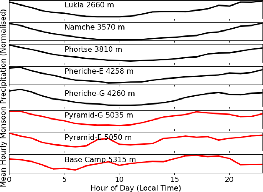
The flattening of this precipitation gradient at higher elevations further up the valley could then be due to local-scale daytime convective winds caused by radiative heating, bringing moist air up the valley, where orographic precipitation will occur in the vicinity of ridges due to convergence. The daytime convective-wind mechanism has been proposed as an explanation for the high precipitation observed close to the termini of some of the smaller glaciers in the Everest region (Ageta, Reference Ageta1976), but an on-glacier peak in precipitation has not been observed for the Khumbu Glacier itself. A precipitation maximum at higher elevations, above the Khumbu Icefall, has previously been speculated (Higuchi and others, Reference Higuchi, Ageta, Yasunari and Inoue1982), but cannot be confirmed due to a lack of observations. Some evidence for the daytime convective winds theory can be found in the diurnal monsoon precipitation patterns seen at increasing altitudes, where a late-afternoon peak in precipitation is evident at higher elevations and not lower in the valley (Fig. 11), similar to the patterns observed in the Langtang Valley (Seko, Reference Seko1987; Baral and others, Reference Baral2014; Shea and others, Reference Shea, Wagnon, Immerzeel, Biron, Brun and Pellicciotti2015a). This late-afternoon precipitation peak at the stations above the elevation of the glacier terminus may be due to the cumulative effect of convective transport of moisture up the valley during daytime radiative heating of the lower valley.
Diurnal patterns of monsoon precipitation at increasing altitudes. Mean hourly precipitation is normalized between 0 and 1 for each station, so that peak timings can be compared independently of overall magnitude. Patterns which exhibit a late-afternoon peak are highlighted in red.

Comparison with mass balance models in GlacierMIP
Results of this study suggest that the factors that affect Khumbu Glacier snow accumulation are largely not captured by global glacier mass balance models, as temperature gradients, precipitation gradients and precipitation phase thresholds calibrated regionally or globally are often inappropriate for this high-altitude summer accumulation glacier. Surveying some of the models included in GlacierMIP shows that these models generally tend to use annual temperature gradients that are too negative, and many use positive precipitation gradients (Table 1). The following discussion highlights the spatio-temporal variation in these modelling parameters and the advantages of using locally derived values rather than regional or global values when modelling accumulation.
GlacierMIP models OGGM, HYOGA2 and GO all use a standard temperature gradient of ∼6.5°C km $^{-1}$. This is more negative than the value of –5.18°C km $^{-1}$ derived in this study for the monsoon, when most accumulation takes place. An overly strong negative gradient will cause the modelled freezing level height to be too low, and therefore the solid precipitation ratio to be too high, leading to an overestimation of accumulation. The regionally calibrated value that JULES applies to South Asia East, –5.32°C km $^{-1}$, is closer to the value derived in this study.
OGGM and HYOGA2 distribute precipitation uniformly over the glacier surface, which appears to be appropriate over the Khumbu Glacier (though not appropriate for glaciers at lower altitudes in the central Himalaya, where a negative gradient would be appropriate). A wide range of positive linear values are used by other models, with +1%/100 m for PyGEM, +2.5%/100 m for GloGEM (applied to the South Asia East region) (PyGEM and GloGEM both also include a function which reduces precipitation exponentially over the top 25% of each glacier with an altitudinal range of over 1000 m), +3%/100 m for Marzeion and others (Reference Marzeion, Jarosch and Hofer2012), and +9%/100 m (for South Asia East) for JULES. Our observations indicate that positive precipitation gradients are inappropriate for the Khumbu and would produce overestimations of annual glacier accumulation. The precipitation–elevation relationship in this region is uncertain at the highest altitudes, but the observations available (both from precipitation gauge and snow pit data) do not support a positive gradient. Non-linearity and spatial heterogeneity of precipitation gradients are also observed in other high-altitude regions such as the Alps (Benoit and others, Reference Benoit, Koch, Peleg and Mariethoz2024).
In terms of precipitation phase thresholds, OGGM and PyGEM both linearly interpolate phase between 0°C and 2°C, and GloGEM linearly interpolates between 0.5°C and 2.5°C. These approaches are fairly consistent with the monsoon values of 0.23°C and 2.17°C derived from the logistic regression, as is the single rain/snow threshold of 1.5°C applied by GO. However, the single rain/snow thresholds of 2°C and 3°C applied by HYOGA2 and Marzeion and others (Reference Marzeion, Jarosch and Hofer2012), respectively, will overestimate the prevalence of snowfall in this region.
The choices of precipitation gradient, temperature gradient, and precipitation phase threshold values have a substantial effect on modelled Khumbu Glacier accumulation (Fig. 9). The mean annual accumulation from this study (575 mm w.e.) is 235 mm w.e. lower than that produced using the parameter values from JULES (810 mm w.e.), a difference of 41%. The lowest annual accumulation total among the GlacierMIP models is from MAR2012, which at 613 mm w.e. is 7% higher than this study. The other models are somewhere between those two, with OGGM, GO, HYOGA2, PyGEM and GloGEM producing annual accumulation totals 8%, 11%, 14%, 24% and 40% higher, respectively, than this study.
Calibration of tuning parameters (e.g., degree day factors, precipitation correction factors) against observations in global-scale models can compensate for modelled accumulation biases to achieve high levels of agreement between observed and simulated (net) mass balance (e.g., Zekollari and others, Reference Zekollari2024). However, projected mass balances could be subject to considerable uncertainty if the primary determinants of accumulation and ablation are not well resolved. Similarly, even if higher-resolution (seasonal) mass balance data are available to constrain modelled accumulation, calibration risks eliminating accumulation errors through the wrong mechanism due to equifinality in model parameters. Matching totals is, therefore, a necessary but not sufficient criterion for modelling the impact of future climate change on glacier mass balance. Reducing uncertainty in model parameters would increase confidence in mass balance projections. Temperature and precipitation gradients are measurable phenomena, and could be calibrated using observations and process-based understanding at glacier, catchment, or regional scales to improve the parameterization of globally applied models. Global-scale glacier modelling studies may improve as new meteorological forcing data products are made available (e.g., Hersbach and others, Reference Hersbach2020; Muñoz-Sabater and others, Reference Muñoz-Sabater2021), but regional biases will persist as long as these crucial accumulation modelling parameters are calibrated at the global scale.
Regional applicability to central Himalayan glaciers
Having demonstrated that the appropriate accumulation modelling parameter values for the Khumbu Glacier are markedly different from the values of worldwide glacier models, it is relevant to consider whether this is true generally of the central Himalayan region, or specific to the Khumbu Valley. To assess this, findings from two other well-observed glacierized catchments in the central Himalaya are compared to the Khumbu.
The Langtang Valley has already been discussed due to some noted similarities it bears to the Khumbu. This is further shown by the temperature gradients presented in Table 4, where it can be seen that seasonal temperature gradients follow a similar pattern to those in the Khumbu. Gradients in the Langtang Valley are least negative during the monsoon, and slightly less negative than they are in the Khumbu Valley. Numerous studies indicate that, in general, precipitation in the Langtang region decreases with elevation from approximately 2500 to 5000 m of elevation, at which point precipitation remains constant, or increases only slightly (Seko, Reference Seko1987; Fujita, Reference Fujita1997; Baral and others, Reference Baral2014; Immerzeel and others, Reference Immerzeel, Petersen, Ragettli and Pellicciotti2014; Collier and Immerzeel, Reference Collier and Immerzeel2015; Bonekamp and others, Reference Bonekamp, de Kok, Collier and Immerzeel2019). This is strikingly similar to the precipitation–elevation relationship in the Khumbu Valley, as shown in Fig. 7.
The Khumbu and Langtang Valleys are located within 100 km of each other, both in the eastern part of the central Himalaya. The Dokriani Glacier catchment, located in northern India, close to the western edge of the central Himalaya, will therefore provide a more distant point of comparison. Three weather stations between 2540 and 4364 m have been collecting meteorological data there since 2011. Temperature gradients there show a similar seasonal pattern to those in the Khumbu and Langtang regions, with the least negative gradient observed during the monsoon, averaging –5.2°C km $^{-1}$ (Pratap and others, Reference Pratap, Dobhal, Bhambri and Mehta2013; Yadav and others, Reference Yadav, Pratap, Gupta, Dobhal, Yadav and Tiwari2019; Reference Yadav, Tiwari, Rai, Shah, Yadav and Kumar2022), close to the –5.23°C km $^{-1}$ Khumbu monsoon value found in this study. This region also exhibits a negative precipitation–elevation relationship, though a more precise pattern cannot be discerned from three stations with an elevational range of less than 2000 m.
The comparisons between these three catchments are supported by wider-scale studies (Table 4). The Nepal-wide temperature gradient study of Kattel and others (Reference Kattel, Yao, Yang, Tian, Yang and Joswiak2013) found a similar pattern of seasonal temperature gradients to those from the Khumbu, Langtang and Dokriani catchments. Whereas temperature gradients seem to be fairly consistent across these three sites and across the central Himalaya more generally, there are sharp contrasts outside this region. Temperature gradients in Bhutan (eastern Himalaya) are similarly less negative during the monsoon, but gradients here are less negative year-round than in the central Himalaya (Kattel and others, Reference Kattel, Yao and Panday2018). In contrast, year-round temperature gradients on the southeastern Tibetan Plateau, on the northern slopes of the Himalaya, exhibit more negative temperature gradients than those found in Nepal and northern India. This suggests that the temperature gradient findings presented in this study may be representative of the central Himalaya, but likely do not have wider relevance for High Mountain Asia, and supports the notion that gradients are related to atmospheric moisture content and the interaction of atmospheric circulation and orographic barriers.
A survey of studies from across the central Himalayan region indicates that precipitation gradients are more variable than temperature gradients. Some central Himalayan studies have identified a double-maximum in precipitation (Bookhagen and Burbank, Reference Bookhagen and Burbank2006; Shrestha and others, Reference Shrestha, Singh and Nakamura2012) with a first maximum below 1000 m of elevation, and a second (lower) maximum at 2100 m. In central and eastern Nepal, a precipitation maximum was found at approximately 2000 m, whereas in western Nepal, a negative precipitation gradient was found over the entire elevation range with maximum precipitation at the lowest elevations (Ichiyanagi and others, Reference Ichiyanagi, Yamanaka, Muraji and Vaidya2007), while precipitation was found to increase with elevation in the western Himalaya and Karakoram (Bonekamp and others, Reference Bonekamp, de Kok, Collier and Immerzeel2019). The above studies are consistent with a physical interpretation that monsoon-dominated regions see negative precipitation gradients between ∼2500 to ∼4000 m of elevation, as orographic forcing at lower elevations removes moisture from monsoonal air masses. Precipitation phase thresholds across the central Himalayas are not known due to a lack of precipitation phase observations.
Longer-term applicability
The parameter values derived from local data in this study are unlikely to be static over the coming decades. Climate change will affect the local and regional physical processes that give rise to the observed temperature and precipitation gradients.
While air temperatures are projected to rise throughout the Himalaya over the 21st century, warming will not be evenly distributed, either spatially or temporally. Temperatures are expected to rise faster at elevations above 3000 m, particularly in the post-monsoon and winter (Dimri and others, Reference Dimri, Kumar, Choudhary and Maharana2018), which will lead to less negative temperature gradients during those seasons. In addition, warmer temperatures at higher altitudes could reduce the elevation-dependent precipitation, which may make precipitation more evenly distributed over the valley elevation range.
Ongoing glacier recession will expose rock surfaces, which may enhance local glacier melt through increased longwave radiation emissions to the glacier surface (Davies and others, Reference Davies2024). Glacier wastage could also potentially increase the concentration of supraglacial debris, which would suppress melt rates (Nicholson and others, Reference Nicholson, Wirbel, Mayer and Lambrecht2021). Glacier recession would also reduce the area over which air temperatures are lowered through sensible and latent heat exchange with the ice surface. These competing processes increase the uncertainty of future changes in temperature and precipitation gradients, and demonstrate the need for modelling parameter values to be updated in step with changing environmental conditions.
Caveats and limitations
The precipitation phase modelling demonstrates the need for more observations of the precipitation phase at a range of altitudes. While the logistic regression modelling based on air temperature was successful, and produced predicted phase probabilities which closely match the observed data, the small altitudinal range (relative to the whole Khumbu Valley) of phase observations (3810–5315 m) available means that the effect of altitude on precipitation phase threshold temperatures in the Khumbu Valley cannot be determined (thresholds in China have been shown to increase with elevation by Zhong and others, Reference Zhong, Zheng, Xu and Qin2018). While phase observations higher than Base Camp are unlikely due to the logistical difficulty in situating a disdrometer above the Khumbu Icefall, phase observations from the lower reaches of the Khumbu Valley would allow for a more robust investigation into the relationships between elevation, air temperature and precipitation phase.
The adjustment of precipitation for wind-induced undercatch comes with a high degree of uncertainty. The choice of catch efficiency transfer function is somewhat arbitrary: this study initially surveyed 26 transfer functions proposed in 12 studies, and that only includes those based on gauge-height wind speed and precipitation phase. Most of these were derived from observations collected at relatively low elevations, where wind speeds are lower on average than in the Khumbu Valley. As a result, many of them are applicable only up to some maximum wind speed, often less than 8 ms $^{-1}$. In the upper part of the Khumbu Valley, wind speeds regularly exceed 10 ms $^{-1}$, and at Pheriche and Pyramid, even daily mean wind speeds have exceeded 8 ms $^{-1}$. In addition, this high-altitude region has lower air density than the sites used to derive the transfer functions. The effect of air density on wind-induced undercatch is unknown, but it will lead to a reduced wind force on falling hydrometeors.
Precipitation rates at the highest elevations remain an open question. The extrapolation of precipitation rates above Base Camp in Fig. 7 is highly speculative due to the lack of observations in the accumulation area. Some confidence in annual snowfall rates at high altitudes can, however, be gleaned from the snow pit data; although these are lower bounds, as the rates of melt and sublimation are unknown. More regular and frequent snow pit observations would strengthen our understanding of Khumbu Glacier accumulation at high elevations, but direct observations of snowfall would provide more certainty (e.g., Pokhrel and others, Reference Pokhrel2024).
The spatial heterogeneity of precipitation in the Khumbu Valley is unresolved by this study. To focus only on the change of rate of precipitation with increasing altitude is to flatten a complex 3-dimensional pattern to the single vertical dimension. Moisture sources change throughout the seasonal cycle, with southerly flow dominating during the monsoon, and westerlies more important through the rest of the year (Perry and others, Reference Perry2020), which may mean that the steep annual negative precipitation gradient seen in the lower Khumbu Valley is a phenomenon exclusive to the monsoon, as it is in the Langtang Valley (Immerzeel and others, Reference Immerzeel, Petersen, Ragettli and Pellicciotti2014). In a region with such extreme heterogeneity of topography, a true understanding of the factors affecting the distribution of precipitation cannot be reached with this simplified approach. Such an approach was chosen here because: a) elevation clearly is an important factor affecting annual precipitation rates, at least in the lower Khumbu Valley (Fig. 7) the distribution of precipitation gauges largely follows the valley transect (Fig. 1) this study aims to arrive at conclusions about accumulation of high-altitude glaciers in the central Himalaya more generally, so a focus on precisely the complexities of the Khumbu Valley is less transferable than the simplified elevation-only approach, which has applicability to other high-altitude central Himalayan glaciers.
Conclusions
Meteorological data from a dense network of high-altitude weather stations in the Khumbu Valley were used to derive local values for accumulation modelling parameters, and to model Khumbu Glacier annual accumulation, as well as its sensitivity to temperature changes. The parameter values derived from the meteorological data were compared to those from previous studies, interpreted in terms of physical processes and assessed for their wider geographical applicability. The parameter values, modelled annual accumulation and temperature sensitivity were compared to those arising from the parameter values of global glacier mass balance models.
This study found that values of temperature gradients, precipitation gradients and precipitation phase temperature thresholds in the GlacierMIP project differ from the values of these parameters appropriate for modelling the accumulation of the Khumbu Glacier, to the extent that glacier-wide accumulation may be overestimated by up to 41%. Significant uncertainties remain in the rates of precipitation at the highest altitudes, and the degree to which precipitation observations are affected by wind-induced undercatch. However, the observations available are sufficient to show that positive precipitation gradients are very likely not applicable to this region, and that the widely used temperature gradient of  $-$6.5°C km $^{-1}$ is too strongly negative, particularly during the monsoon when most accumulation occurs. The values of these parameters have a critical impact on the modelling of accumulation, and using existing model values rather than calibrating from local data produces modelled Khumbu Glacier accumulation that is too high, and less sensitive to warming temperatures. The parameter values appropriate for the Khumbu Valley are physically interpretable and likely to be more widely applicable across the region, particularly the seasonal temperature gradients, and perhaps the precipitation gradient, at least for the eastern part of the central Himalaya.
Supplementary material
The supplementary material for this article can be found at https://doi.org/10.1017/jog.2026.10147.
Data availability statement
Publicly available meteorological data from the following sources were used: National Geographic and Rolex Perpetual Planet Everest Expedition (https://www.nationalgeographic.org/society/everest-weather-data/), National Observation Service GLACIOCLIM (CNRS-INSU program, OSUG, IRD, INRAE, IPEV, Météo France) (https://glacioclim.osug.fr/Donnees-himalaya), Ev-K2-CNR geoportal (https://geoportal.mountaingenius.org/portal/), Coordinated Energy and Water Cycle Observations Project (CEOP) (https://search.diasjp.net/en/dataset/CEOP_CAMP_Himalayas) and Rowan and others (Reference Rowan, Quincey, Gibson and Irvine-Fynn2017) (https://doi.org/10.1594/PANGAEA.883071).
Acknowledgements
Supplementing the above publicly available data, additional data were provided by the following contributors: disdrometer data from Pyramid-G by Patrick Wagnon, Guilhem Freche and Michel Esteves, precipitation and temperature data from the Paprika-Preshine stations by Pierre Chevallier (Chevallier and others, Reference Chevallier2017), precipitation data from the Nepal DHM gauge at Chaurikharka by Nirakar Thapa and wind data from Base Camp, plus the most recent National Geographic data and the snow pit data, by Tom Matthews and Baker Perry. We thank Joseph Shea and two anonymous reviewers for their helpful, clear and thorough comments.






 Open access

