2.1 Technology

The consumption-goods sector $(x)$ and the investment-goods sector $(y)$ operate time-invariant constant-returns-to-scale production technologies given by the production functions

\begin{equation*} f_j \, : \, \mathbb{R}_+ \to \mathbb{R}_+,\quad k^j \mapsto f_j(k^j),\quad j=x,y, \end{equation*}

where $k^j$ denotes the capital intensity in sector $j$ . The sector-specific marginal products of labour and capital are $w_j(k^j)\,:\!=\,f_j(k^j)-f^{\prime }_j(k^j)k^j$ and $f_j^\prime (k^j)$ , respectively, so that the corresponding marginal rates of technical substitution (MRTS) take the form

(1) \begin{equation} \Omega _j(k^j)\,:\!=\,\frac {w_j(k^j)}{f_j^\prime (k^j)}=\frac {f_j(k^j)}{f_j^\prime (k^j)}-k^j,\quad j=x,y. \end{equation}

Assumption1 dates back to Drandakis (Reference Drandakis1963).Footnote ¹ It follows from Assumption1 (i) that the MRTS functions $\Omega _x$ and $\Omega _y$ are continuously differentiable and strictly increasing. Assumption1 (ii) ensures that there exist continuously differentiable relative factor demand functions $\kappa _j \, : \, \mathbb{R}_{+} \to \mathbb{R}_{+}$ , $j=x,y$ , defined by

(2) \begin{equation} \Omega _j(\kappa _j(\omega ))=\omega \quad \text{for all }\,\omega \in \mathbb R_+. \end{equation}

These functions determine the sector-specific capital-to-labour ratios $\kappa _j(\omega )$ , given a wage-rental ratio $\omega$ . Factor-intensity reversals arise if $\Omega _x$ and $\Omega _y$ intersect. Specifically, if $\Omega _x(k)\lt \Omega _y(k)$ , then

(3) \begin{equation} \kappa _y(\omega )\lt k\lt \kappa _x(\omega ) \quad \text{for all }\, \omega \in \bigl (\Omega _x(k),\Omega _y(k)\bigr ). \end{equation}

Vice versa, if $\Omega _x(k)\gt \Omega _y(k)$ , then

(4) \begin{equation} \kappa _x(\omega )\lt k\lt \kappa _y(\omega ) \quad \text{for all }\, \omega \in \big (\Omega _y(k),\Omega _x(k)\bigr ). \end{equation}

The class of production functions with a constant elasticity of factor substitution (CES) satisfies Assumption1. This class features factor-intensity reversals and, in general, violates one of the Inada (Reference Inada1963) conditions, a rather restrictive property typically assumed in the literature.

For any wage-rental ratio $\omega$ , the production elasticity in sector $j$ is determined by a function $\varepsilon _j\, : \, \mathbb R_{++}\to \mathbb R$ , defined by

\begin{equation*} \varepsilon _j(\omega ) \,:\!=\,\frac {f_j^\prime (\kappa _j(\omega ))\kappa _j(\omega )}{f_j(\kappa _j(\omega ))}. \end{equation*}

The elasticity of factor substitution in sector $j$ is determined by the function $\sigma _j\, : \, \mathbb R_{++}\to \mathbb R_+$ , defined byFootnote ²

(5) \begin{equation} \sigma _j(\omega )\,:\!=\,\frac {\kappa _j^\prime (\omega )\omega }{\kappa _j(\omega )}. \end{equation}

Example 1 (CES production functions). CES production functions $f_j\, : \, \mathbb R\to \mathbb R_+$ are defined by

(6) \begin{align} f_j(k) = \left \{ \begin{array}{l@{\quad \mbox{if}\ }l} \displaystyle \frac {a_j}{b_j}\ k^{b_j} & \sigma _j=1 \\ \displaystyle \frac {a_j}{b_j} \left [b_j k^{\frac {\sigma _j-1}{\sigma _j}} +(1-b_j)\right ]^{\frac {\sigma _j}{\sigma _j-1}} & \sigma _j \neq 1 \end{array} \right ., \end{align}

where $a_j\gt 0$ scales the total factor productivity, $0\lt b_j \lt 1$ stipulates the factor-income distribution, and $\sigma _j\gt 0$ determines the constant elasticity of factor substitution. The case of Cobb–Douglas production functions, $\sigma _j=1$ , is the only case in which both Inada conditions are satisfied. The MRTS functions $\Omega _j \, : \, \mathbb{R}_+\to \mathbb{R}_+$ , $j=x,y$ take the form

\begin{equation*} \Omega _j(k)=\dfrac {1-b_j}{b_j}k^{\dfrac {1}{\sigma _j}}. \end{equation*}

The relative factor demand functions $\kappa _j\, : \, \mathbb R_+\to \mathbb R_+$ , $j=x,y$ are

(7) \begin{equation} \kappa _j(\omega )=\left (\dfrac {b_j}{1-b_j}\omega \right )^{\sigma _j}. \end{equation}

Unless $\sigma _x=\sigma _y$ , exactly one factor-intensity reversal occurs at

\begin{equation*} \overline {\omega }\,:\!=\, \left (\dfrac {b_x}{1-b_x}\right )^{\frac {\sigma _x}{\sigma _y-\sigma _x}} \left (\dfrac {1-b_y}{b_y}\right )^{\frac {\sigma _y}{\sigma _y-\sigma _x}}. \end{equation*}

Specifically, for $\sigma _x\lt \sigma _y$ ,

\begin{equation*} \kappa _y(\omega )\gtreqless \kappa _x(\omega ) \iff \omega \gtreqless \overline \omega , \end{equation*}

where $\overline {k}=\kappa _x(\overline {\omega })=\kappa _y(\overline {\omega })$ is the critical value at which the factor intensities revert.

2.2 Temporary equilibria

A feasible allocation in period $t$ is a list of relative factor inputs $(k^x_t,k^y_t, l^x_t,l^y_t)\geq 0$ that satisfies

(8) \begin{equation} l_t^x + l_t^y=1 \quad \text{and}\quad l_t^x k_t^x + l_t^y k_t^y=k_t, \end{equation}

where $l^x_t\,:\!=\,\frac {L^x_t}{L_t}$ and $l^y_t\,:\!=\,\frac {L^y_t}{L_t}$ are the sector-specific labour shares, $k^x_t$ and $k^y_t$ the sector-specific capital-to-labour ratios, and $k_t=\frac {K_t}{L_t}$ is the economy-wide capital-to-labour ratio. A temporary equilibrium in period $t$ is a feasible allocation $(k_t^x,k_t^y, l_t^x,l_t^y)$ together with prices $(r_t,w_t,p_t)$ denominated in the investment good at which all markets clear and profits in both sectors a maximised.

Since capital and labour are allowed to move frictionless, both sectors must pay the same factor prices. The first-order conditions for profit maximisation are

(9) \begin{equation} p_t f'_x(k^x_t)=f'_y(k^y_t)=r_t \quad \text{and}\quad p_tw_x(k^x_t)= w_y(k^y_t)=w_t. \end{equation}

Denote output per unit of aggregate labour input in sector $j=x,y$ by $x_t= l^x_tf_x(k^x_t)$ and $y_t=l^y_tf_y(k^y_t)$ , respectively. Given the exogenous savings propensity $0\leq s\leq 1$ , the market-clearing condition in the investment-goods market is

(10) \begin{equation} s[w_t+r_tk_t]=l^y_tf_y(k^y_t) \end{equation}

and the market-clearing condition in the consumption-goods market is

(11) \begin{equation} (1-s)[w_t+r_tk_t]=p_t l^x_t \, f_x(k^x_t). \end{equation}

It follows from Assumption1 that for any feasible allocation (8) at prices $(r_t,w_t,p_t)$ that satisfies (9), aggregate factor income is equal to the value of aggregate output, that is,

(12) \begin{equation} w_t+r_tk_t=p_tx_t+y_t. \end{equation}

A temporary equilibrium may now be characterised as follows. Denoting the wage-rental ratio by $\omega _t=\frac {w_t}{r_t}$ , the first-order conditions (9) may be rewritten as

(13) \begin{equation} \Omega _x(k^x_t)=\Omega _y(k^y_t)=\omega _t \quad \text{and}\quad \frac {f_y^\prime (k^y_t)}{f_x^\prime (k^x_t)}=p_t. \end{equation}

The relative factor demand functions (2) fulfil the first equation in (13) by construction, so that $k^j_t=\kappa _j(\omega _t)$ , $j=x,y$ for any $\omega _t\in \mathbb R_+$ . As a consequence, all equilibrium prices become functions of the wage-rental ratio, so that

(14) \begin{equation} r_t=f_y^\prime (\kappa _y(\omega _t)),\quad w_t=w_y(\kappa _y(\omega _t)), \quad \text{and}\quad p_t= p_x(\omega _t)\,:\!=\,\frac {f_y^\prime (\kappa _y(\omega _t))}{f_x^\prime (\kappa _x(\omega _t))}. \end{equation}

Given an economy-wide capital-to-labour ratio $k_t\in \mathbb R_+$ , there are two cases, the ‘generic’ case $\Omega _x(k_t)\neq \Omega _y(k_t)$ and the ‘non-generic’ case $\Omega _x(k_t)=\Omega _y(k_t)$ . Following Ritschel and Wenzelburger (Reference Ritschel and Wenzelburger2024), for each $k_t\in \mathbb R_+$ , set

\begin{equation*} \Omega _{\mathrm{min}}(k_t)\,:\!=\,\min \bigl \{\Omega _x(k_t),\Omega _y(k_t)\bigr \} \quad \text{and}\quad \Omega _{\mathrm{max}}(k_t)\,:\!=\,\max \bigl \{\Omega _x(k_t),\Omega _y(k_t)\bigr \}. \end{equation*}

For each $k_t\gt 0$ with $\Omega _x(k_t)\not =\Omega _y(k_t)$ , define the two sector-specific labour-share functions

(15) \begin{equation} \ell _j(k_t,\cdot) \,:\, [\Omega _{\mathrm{min}}(k_t),\Omega _{\mathrm{max}}(k_t)] \to [0,1], \quad j=x,y, \end{equation}

by setting

\begin{equation*} \ell _x(k_t,\omega ) =\frac {\kappa _y(\omega )-k_t}{\kappa _y(\omega )-\kappa _x(\omega )} \quad {and}\quad \ell _y( k_t,\omega ) =\frac { k_t-\kappa _x(\omega )}{\kappa _y(\omega )-\kappa _x(\omega )}, \end{equation*}

respectively.Footnote ³ It is straightforward to verify that any list

\begin{equation*} \bigl (\kappa _x(\omega _t),\kappa _y(\omega _t),l_x(k_t,\omega _t),l_y(k_t,\omega _t)\bigr ) \,\text{with}\, \bigl (f_y^\prime (\kappa _y(\omega _t)),w_y(\kappa _y(\omega _t)), p_x(\omega _t)\bigr ), \end{equation*}

where $\omega _t\in \bigl [\Omega _{\mathrm{min}}(k_t),\Omega _{\mathrm{max}}(k_t)\bigr ]$ , fulfils (8) and (9) and hence is a feasible factor allocation. The remaining market-clearing conditions (10) and (11) in the two goods markets are satisfied as follows. For any $k_t$ with $\Omega _x(k_t)\neq \Omega _y(k_t)$ , define the excess demand function for investment goods $T(k_t,\cdot ) \, : \, \bigl [\Omega _{\mathrm{min}}(k_t),\Omega _{\mathrm{max}}(k_t)\bigr ]\to \mathbb R,$ by setting

(16) \begin{equation} T(k_t,\omega )\,:\!=\, s\bigl [w_y(\kappa _y(\omega ))+f_y'(\kappa _y(\omega ))k_t\bigr ] -\ell _y(k_t,\omega )f_y(\kappa _y(\omega )). \end{equation}

Invoking Walras’ law, the next lemma provides a characterisation of temporary equilibria.

Lemma1 states that a temporary equilibrium is determined by a wage-rental ratio $ \Omega _{\mathrm{min}}(k_t) latbreak{} \leq \omega _t\leq \Omega _{\mathrm{max}}(k_t)$ for which the market for investment goods clears. In the non-generic case, the labour share in the investment-goods market is $l^y_t=s$ .

Since a temporary equilibrium in period $t$ is uniquely determined by the wage-rental ratio $\omega _t=\Omega (k_t)$ , will refer to $\Omega$ as the temporary equilibrium map of the economy. We show in Lemma6, Appendix A.1 that $\Omega$ is differentiable.

Example 2 (Temporary equilibria for CES production functions). Let $k_t\neq \overline {k}$ , with $\overline {k}$ as defined in Example 1 , be given and $\omega _t$ be the equilibrium wage-rental ratio. The equilibrium factor allocation obtains from inserting the corresponding capital-to-labour ratios (7) into the labour-share functions (15). For $\sigma _x\neq 1$ and $\sigma _y\neq 1$ , the equilibrium wage and rental rate are

(18) \begin{align} \begin{aligned} w_y(\kappa _y(\omega _t))&= \dfrac {a_y}{b_y}\left (b_y^{\sigma _y}\omega _t^{\sigma _y-1}+(1-b_y)^{\sigma _y}\right )^\frac {1}{\sigma _y-1} \\ f_y^\prime (\kappa _y(\omega _t))&= \dfrac {a_y}{b_y}\left (b_y^{\sigma _y}+(1-b_y)^{\sigma _y}\omega _t^{1-\sigma _y}\right )^\frac {1}{\sigma _y-1}. \end{aligned} \end{align}

The consumption-goods price is

(19) \begin{equation} p_x(\omega _t)= \frac {\frac {a_y}{b_y}\Bigl (\alpha _y^{\sigma _y}+(1-b_y)^{\sigma _y}\omega _t^{1-\sigma _y} \Bigr )^\frac {1}{\sigma _y-1}} {\frac {a_x}{b_x}\Bigl (b_x^{\sigma _x}+(1-b_x)^{\sigma _x}\omega _t^{1-\sigma _x} \Bigr )^\frac {1}{\sigma _x-1}}. \end{equation}

2.3 Capital accumulation

Applying the identity (2) twice, aggregate factor income per capita at any $(k,\omega )\in \mathbb R_{++}^2$ satisfies

(20) \begin{align} w_y(\kappa _y(\omega ))+f_y^\prime (\kappa _y(\omega ))k & =[\omega +k]f_y^\prime (\kappa _y(\omega )) =\left [\frac {\omega +k}{\omega +\kappa _y(\omega )}\right ] f_y(\kappa _y(\omega )). \end{align}

The economy’s propensity to invest in a temporary equilibrium may now be defined as a function of the economy-wide capital intensity $\mathcal S\, : \, \mathbb R_+\to \mathbb R_+$ by settingFootnote ⁴

(21) \begin{equation} \mathcal S(k)\,:\!=\,s\left [ \frac {\Omega (k)+k}{\Omega (k)+\kappa _y(\Omega (k))}\right ]. \end{equation}

Market clearing requires the propensity to invest to be equal to the labour share of the investment-goods sector, so that

(22) \begin{align} \mathcal S(k)= \begin{cases} \ell _y(k,\Omega (k))&\text{if }\,\Omega _x(k)\neq \Omega _y(k) \\ s&\text{if }\,\Omega _x(k)=\Omega _y(k) \end{cases}. \end{align}

Assuming that capital depreciates at the rate $0 \leq \delta \leq 1$ and that labour supply grows at the rate $n\gt -1$ so that $L_{t+1}=(1+n)L_t$ , the capital-to-labour ratio in period $t+1$ is equal to the sum of depreciated capital and investments in period $t$ . Given an initial capital-to-labour ratio $k_0\geq 0$ , the evolution of the capital-to-labour ratios $k_t=\frac {K_t}{L_t}$ is thus governed by the time-one map $G\, : \, \mathbb R_{+}\to \mathbb R_{+}$ , defined by

(23) \begin{equation} k_{t+1}=G(k_t)\,:\!=\, \tfrac {1}{1+n} \bigl [(1-\delta )k_t +\mathcal S(k_t)f_y(\kappa _y(\Omega (k_t)))\bigr ],\quad t\geq 0. \end{equation}

We will show next that our parsimonious growth model (23) allows for multiple steady states, cycles of any order, and complex dynamics. Since the maps $f_y$ , $\kappa _y$ , and $\Omega$ are all strictly increasing, all non-linearities of the map $G$ must originate from the economy’s propensity to invest $\mathcal S$ .

Lemma 2 (Properties of $\mathcal S$ ). The propensity to invest $\mathcal S$ takes the form

(24) \begin{equation} \mathcal S(k)=\frac {s}{s+(1-s)h(\Omega (k))},\quad k\in \mathbb R_{++}, \end{equation}

where $h\, : \, \mathbb R_{++}\to \mathbb R_+$ is defined by

(25) \begin{equation} h(\omega )\,:\!=\,\frac {\omega +\kappa _y(\omega )}{\omega +\kappa _x(\omega )}. \end{equation}

Moreover, $\mathcal S^\prime (k)\lt 0$ if and only if $h^\prime (\Omega (k))\gt 0$ .

In the proof of Lemma2 in Appendix A.1, we will show with equation (50) that the function $h$ may be rewritten as

(26) \begin{equation} h(\omega )=\frac {f_y(\kappa _y(\omega ))}{ p_x(\omega ) f_x(\kappa _x(\omega ))} =\frac {1-\varepsilon _x(\omega )}{1-\varepsilon _y(\omega )}, \quad \omega \in \mathbb R_{++}. \end{equation}

Thus, Lemma2 implies that the propensity to invest is a decreasing function of the economy-wide capital-to-labour ratio whenever the investment-good output $f_y(\kappa _y(\omega ))$ increases faster with an increase in the wage-rental ratios than the value of the consumption-good output $p_x(\omega )f_x(\kappa _x(\omega ))$ . Stated differently, a price effect is responsible for a decreasing propensity to invest. It follows from (22) that the equilibrium labour-share of the investment-goods sector must then be a non-increasing function of the capital-to-labour ratio.Footnote ⁵ The classical one-sector Solow–Swan growth model excludes such a nonlinearity because the propensity to invest is constant. With two sectors, investment is solely generated out of income earned in the investment-goods sector and (20) shows that factor incomes no longer add up to output of that sector. Therefore, a negative effect of an increase in $k$ on capital income may dominate the positive effect on labour income.

Example 3 (Propensity to invest for CES production functions). Suppose that both production functions are of the CES type specified in Example 1 . Inserting the capital intensities (7) into (25) yields

(27) \begin{equation} h(\omega ) =\frac {1+\left (\frac {b_y}{1-b_y}\right )^{\sigma _y}\omega ^{\sigma _y-1}} {1+\left (\frac {b_x}{1-b_x}\right )^{\sigma _x}\omega ^{\sigma _x-1}}. \end{equation}

Since by Lemma 6 , Appendix A.1 the temporary equilibrium map $\Omega$ is strictly increasing, it follows from (27) that for $\sigma _x\lt 1\leq \sigma _y$ , the propensity to invest $\mathcal S$ is strictly decreasing with $\lim _{k\to 0}\mathcal S(k)=1$ . This case, therefore, has the potential for non-monotonic time-one maps $G$ . For $\sigma _x\geq 1\geq \sigma _y$ , the propensity to invest $\mathcal{S}$ is non-decreasing. The corresponding time-one maps $G$ will therefore be strictly increasing. In Section 3 below, it will be shown that $G$ is strictly increasing whenever $\sigma _x\geq 1$ . The analysis of the remaining case $\sigma _x,\sigma _y\lt 1$ is tedious and must be considered elsewhere.

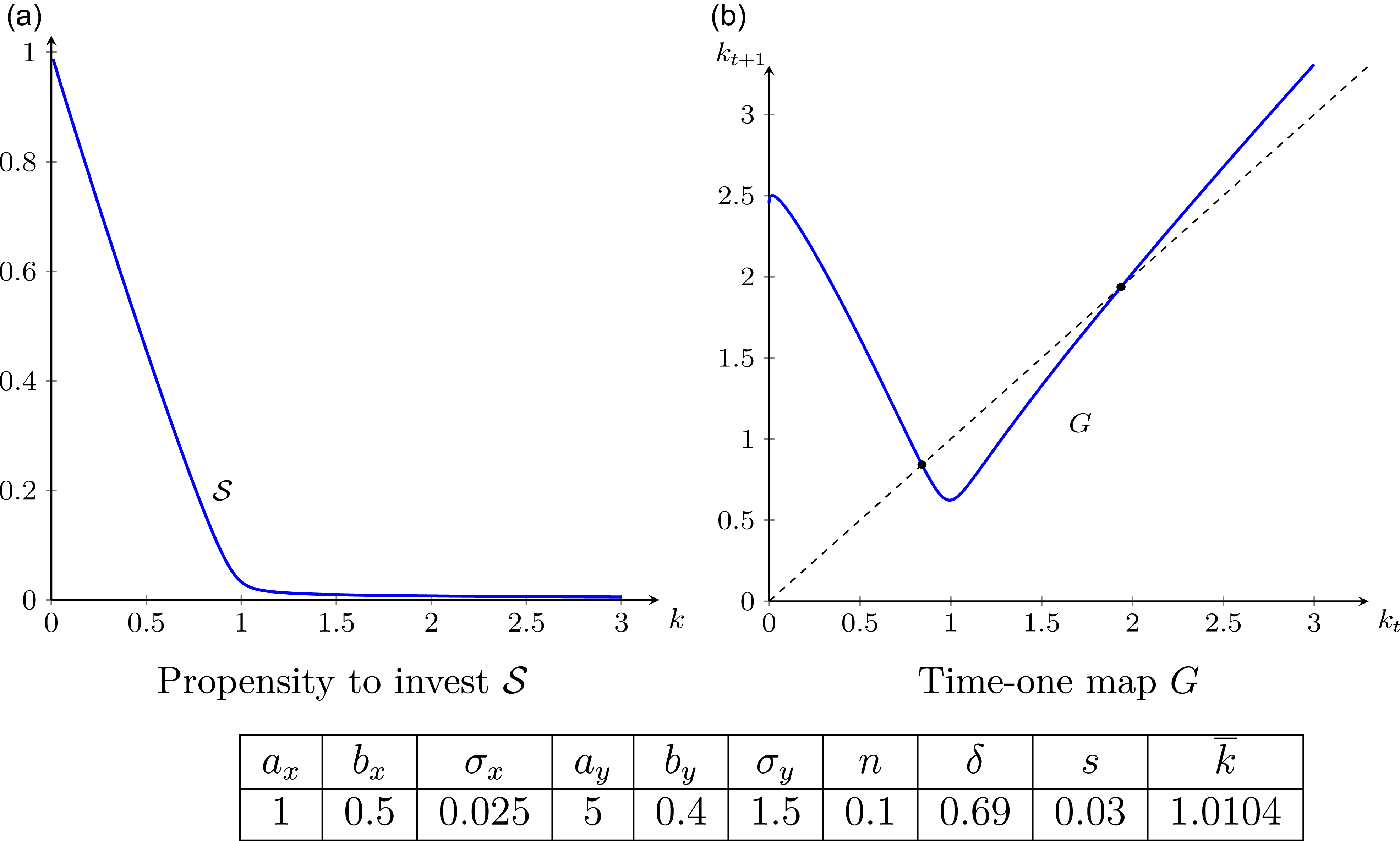
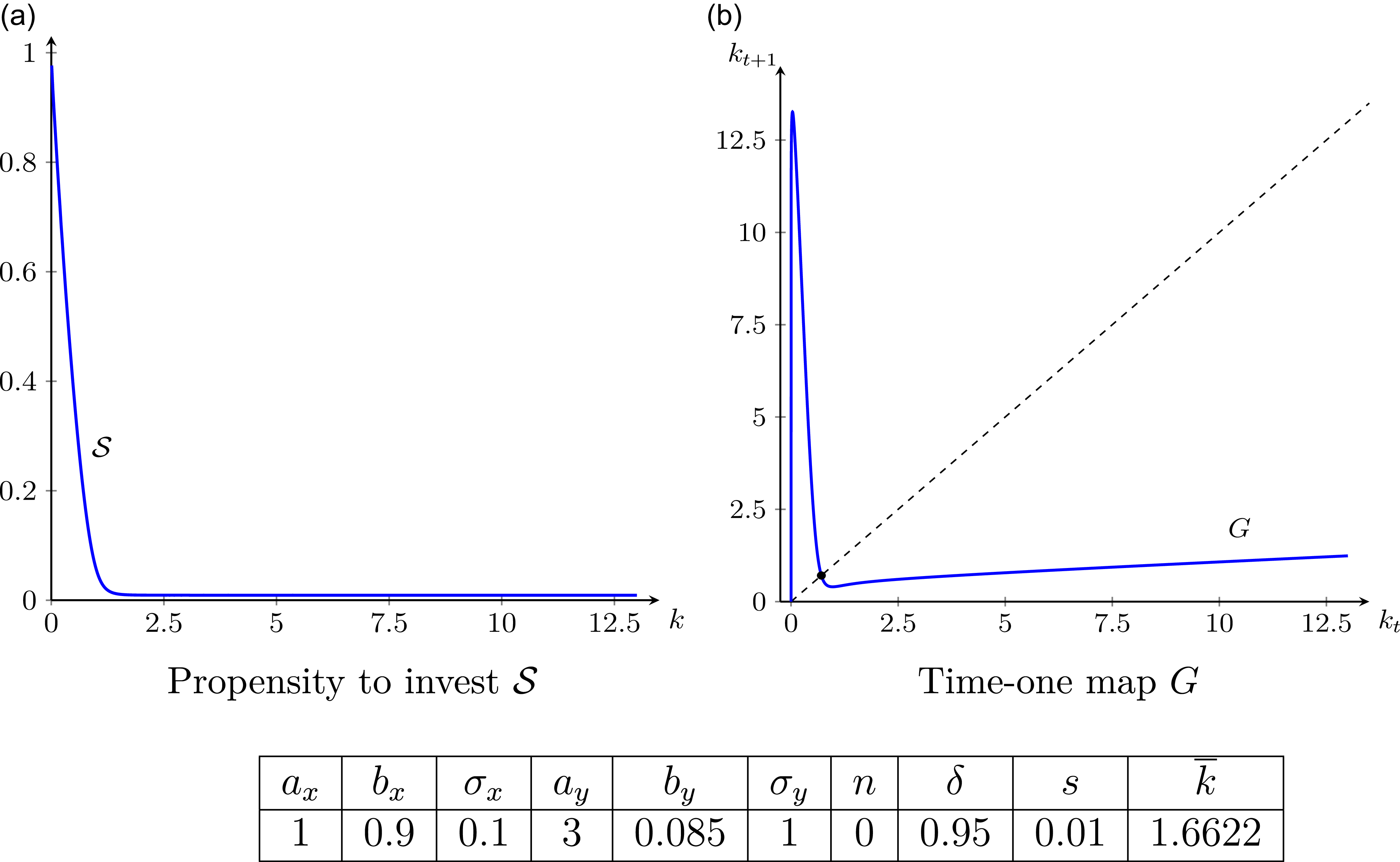
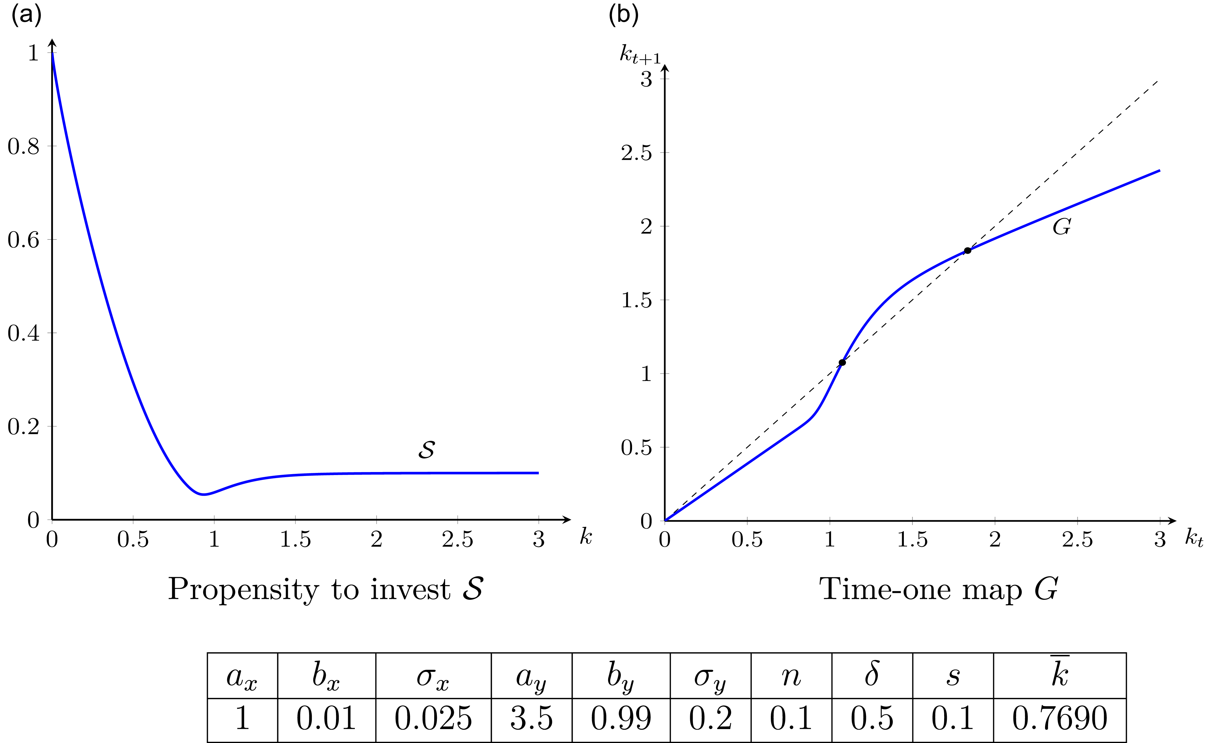
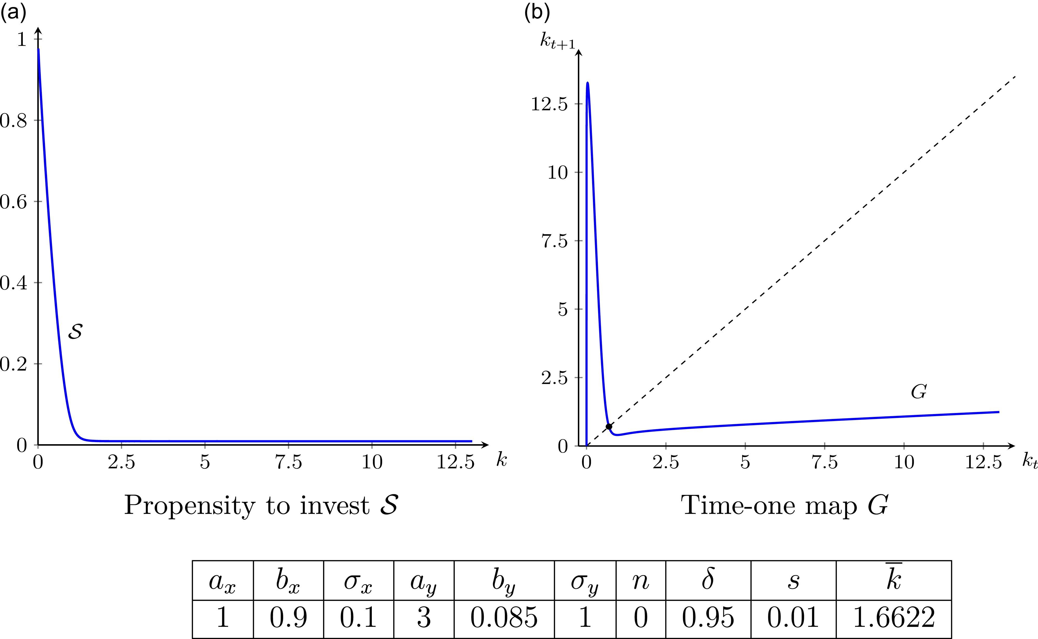
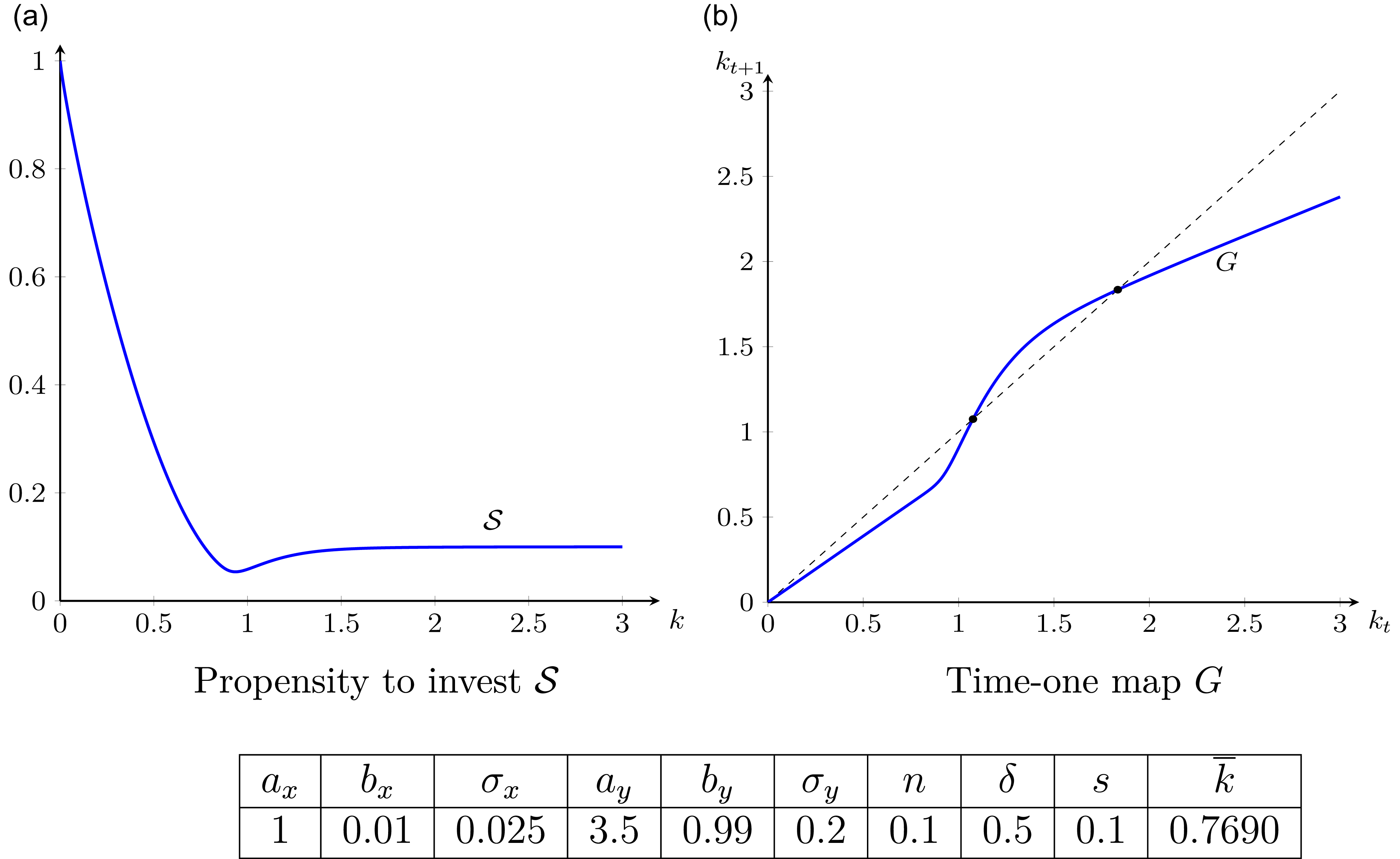
Example3 is illustrated in Figures 1–3 with three specific parametrisations of CES production functions. These figures show that non-monotonic time-one maps $G$ obtain whenever $\mathcal S$ is decreasing sufficiently fast. Figures 1 and 2 portray two parametrisations with non-monotonic time-one maps $G$ ; Figure 3 portrays a parametrisation in which $\mathcal S$ may be decreasing while $G$ is nevertheless increasing. Since in all three cases $\sigma _x\lt \sigma _y$ , we know from Example1 that the investment-goods sector is more capital intensive for all $k$ above the critical value $\overline k$ . The figures suggest that $G$ is increasing for $k\gt \overline k$ in all three cases.

Figure 1.

Case A. CES production functions, $\sigma _x\lt 1\lt \sigma _y$ .

Figure 2.

Case B. CES production functions, $\sigma _x\lt \sigma _y=1$ .

4.1 Steady states, development trap, and unbounded growth

For CES production functions, the map $\phi$ defined in (29) takes an analytically tractable form so that all theoretical results of Section 3 can be applied. The limits for the marginal products (32) suggest to distinguish between three cases: $\sigma _y\lt 1$ , $\sigma _y\gt 1$ , and $\sigma _y=1$ . For $\sigma _y\neq 1$ , two mutually exclusive sets of model parameters $(b_x,\sigma _x,a_y,b_y,\sigma _y,n,\delta ,s)$ turn out to be crucial. First, the case

(36) \begin{align} \frac {n+\delta }{a_yb_y^\frac {1}{\sigma _y-1}} \lt \begin{cases} s&\text{if }\, \sigma _x\lt 1 \\ \dfrac {s}{(1-b_x)s+b_x} &\text{if }\,\sigma _x=1 \\ 1&\text{if }\, \sigma _x\gt 1 \end{cases}. \end{align}

Second, the case

(37) \begin{align} \frac {n+\delta }{a_yb_y^\frac {1}{\sigma _y-1}} \gt \begin{cases} s&\text{if }\, \sigma _x\lt 1 \\ \dfrac {s}{(1-b_x)s+b_x} &\text{if }\,\sigma _x=1 \\ 1&\text{if }\, \sigma _x\gt 1 \end{cases}. \end{align}

Observe that the factor productivity $a_x$ of the consumption-goods sector does not appear in the above expressions. From Example2, we infer that any change in $a_x$ affects solely output quantity and price of the consumption good.

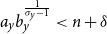
Proposition2 states that for $\sigma _y\lt 1$ , a positive steady state exists whenever the savings propensity $s$ and/or the factor productivity $a_y$ are sufficiently large. Since $f_y(0)=0$ , capital is an essential input for producing investment goods so that the origin is a steady state. A development trap obtains whenever the savings propensity and/or the factor productivity $a_y$ is too low so that Condition (37) is satisfied. Figure 3b portrays an example with an asymptotically stable origin and two positive steady states. Since Condition (37) holds, this example shows that Condition (36) is sufficient but not necessary for the existence of positive steady states. If the factor productivity is too low, then no positive steady state exists and the development trap is globally asymptotically stable.

Proposition3 states that for $\sigma _y\gt 1$ , a positive steady state exists whenever the savings propensity $s$ and/or the factor productivity $a_y$ is not too large. Condition (36) implies that except for the case $\sigma _x\gt 1$ , unbounded growth occurs if the savings propensity $s$ in relation to factor productivity $a_y$ is sufficiently large. The origin is not a steady state, because capital is not essential for producing investment goods. The example portrayed in Figure 1b demonstrates that Condition (37) is sufficient but not necessary. The time-one map $G$ has two positive steady states even though Condition (37) is violated and unbounded growth is possible.

Lemma5 states that neither a development trap nor unbounded growth is possible if the output of the investment-goods sector is determined by a Cobb–Douglas production function. This case is illustrated in Figure 2b, which depicts a time-one map $G$ with a hump.

An immediate consequence of the last three results is the following corollary, which summarises conditions under which the dynamics are qualitatively indistinguishable from the dynamics of the classical Solow–Swan model.

Corollary 1. Consider the case with CES production functions ( 6 ) and let $\sigma _x\geq 1$ . Then $G^\prime \gt 0$ . If, in addition, one of the following three conditions,

\begin{equation*} (i)\quad \sigma _y=1,\quad (ii)\quad \sigma _y\lt 1\, and \ (36) \ holds, \quad or \,\quad (iii)\quad \sigma _y\gt 1\, and \ (37) \ holds, \end{equation*}

is satisfied, then there exists a uniquely determined positive steady state $G(k^\ast )=k^\ast \gt 0$ , which is asymptotically stable on $\mathbb R_{++}$ .

4.2 Numerical evidence for complex dynamics

The simulation results presented next provide numerical evidence for complex dynamics if the substitution elasticity $\sigma _x$ is sufficiently small.Footnote ⁶

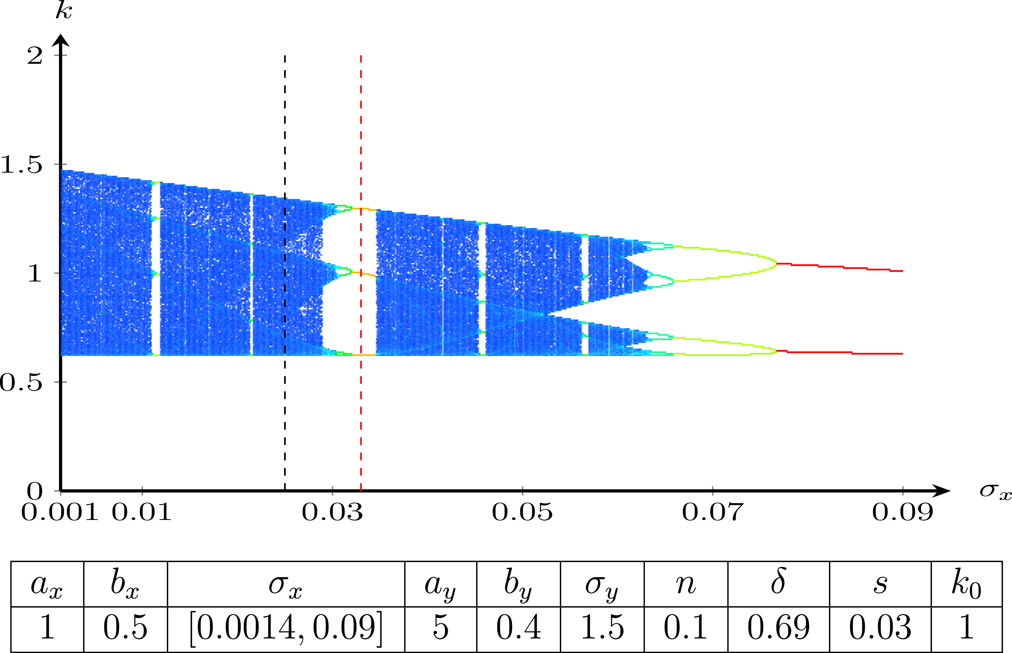
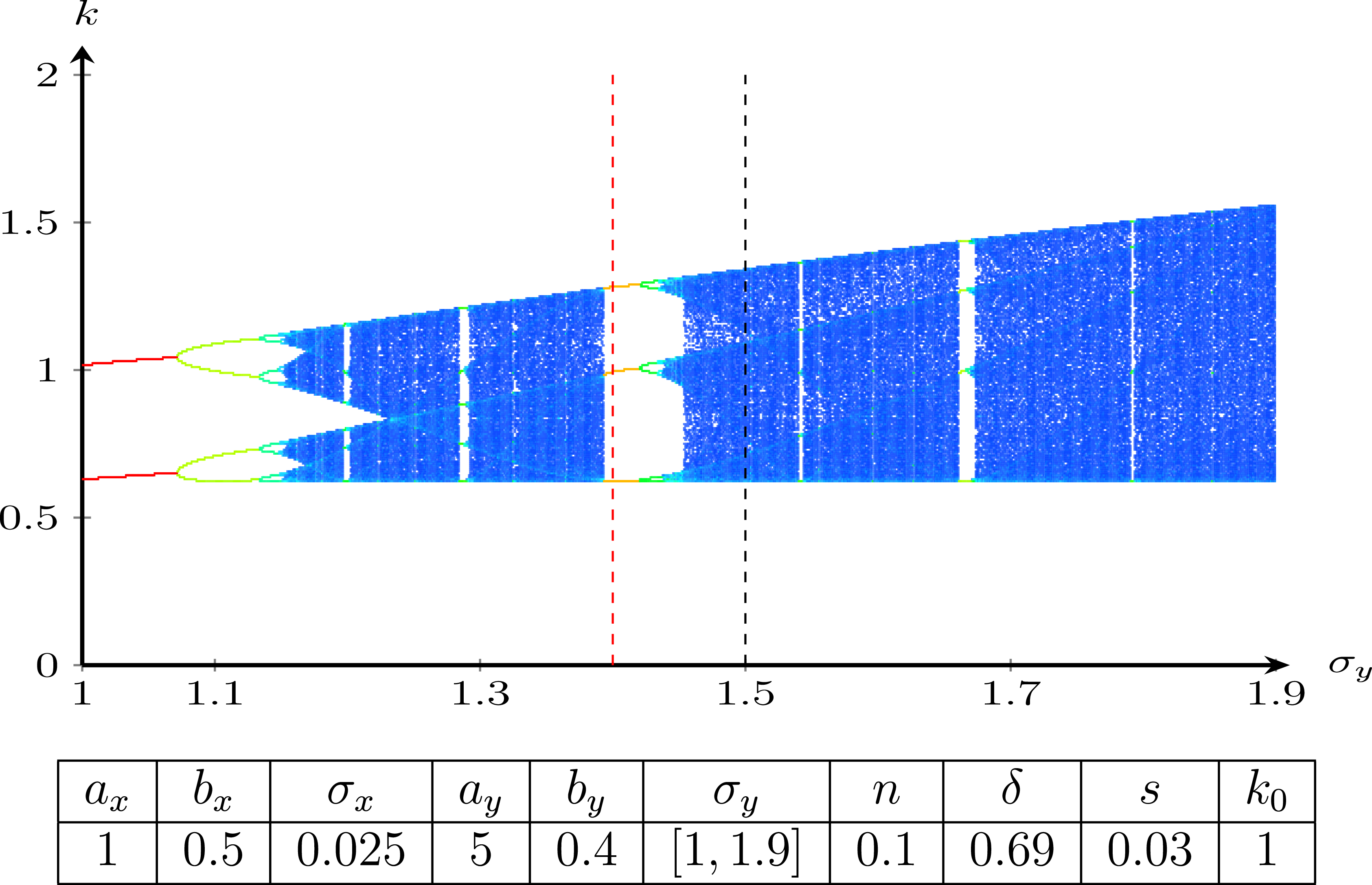
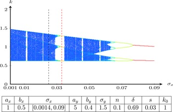
Figure 1 shows that the time-one map $G$ in Case A has at least two positive steady states, which are both unstable. By Proposition3, the origin is not a steady state and unbounded growth obtains for all sufficiently large initial values. All growth paths $\{k_t\}_{t=0}^{\infty }$ with initial values $k_0$ below the larger steady state are bounded. For the initial value $k_0=1$ , the bifurcation diagrams in Figures 4 and 5 illustrate how changes in the elasticities of factor substitution affect the qualitative dynamics. The growth path corresponding to $\sigma _x=0.025$ in Figure 4 provides numerical evidence that the model exhibits non-periodic business cycles. For $\sigma _x=0.033$ , Figure 4 shows that the growth path starting in $k_0=1$ converges to a period-3 cycle. Similarly for $\sigma _y=1.4$ instead of $\sigma _y=1.5$ , Figure 5 shows that the growth path starting in $k_0=1$ converges to a period-3 cycle as well. By Li and Yorke (Reference Li and Yorke1975), the period-3 cycles ensure the presence of topological chaos, implying that cycles of any order and irregular fluctuations exist.

Figure 4.

Case A. Bifurcation over the substitution elasticity $\sigma _x$ .

Figure 5.

Case A. Bifurcation over the substitution elasticity $\sigma _y$ .

Figure 6.

Case A. Bifurcation over the savings propensity $s$ .

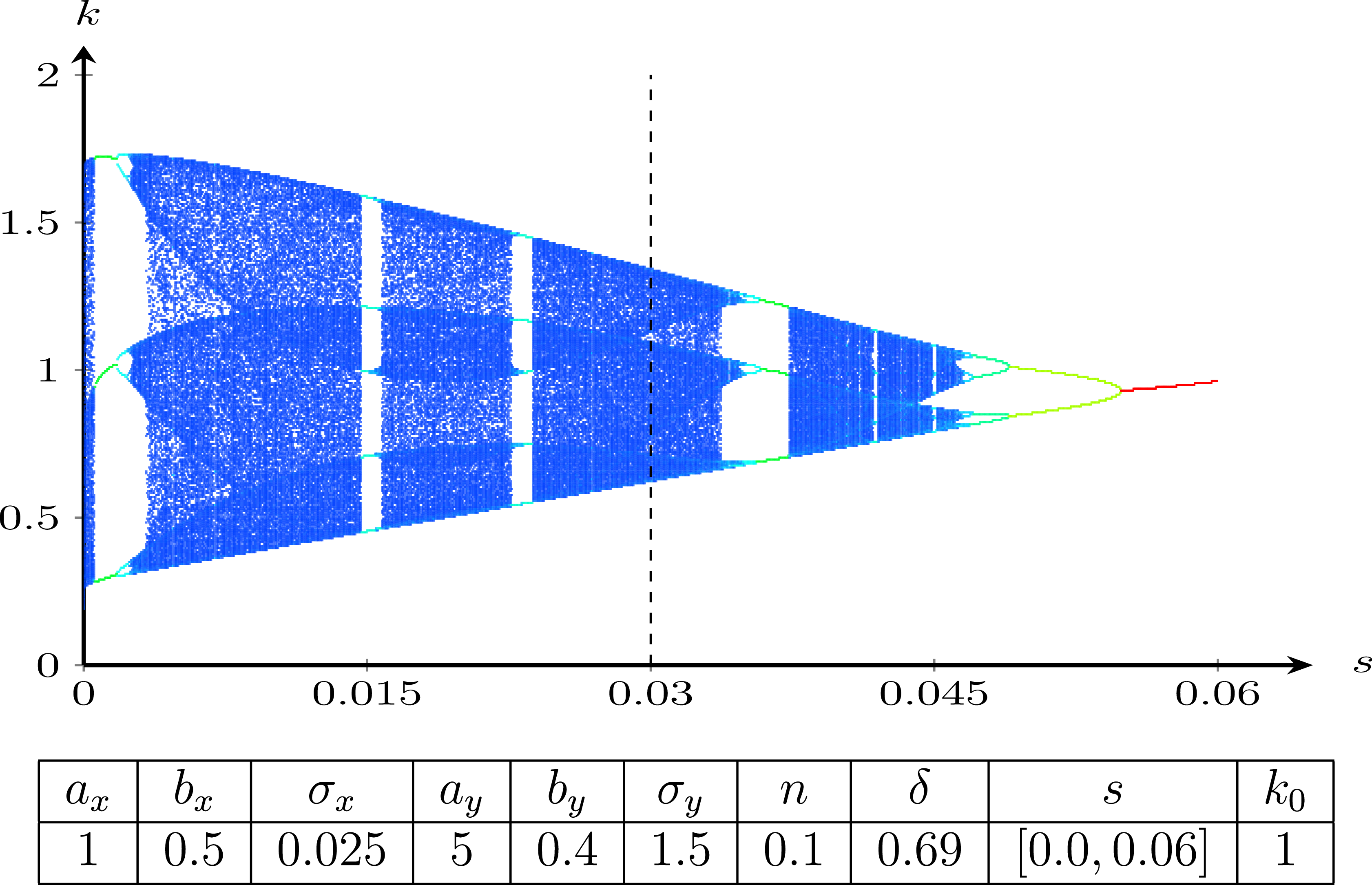
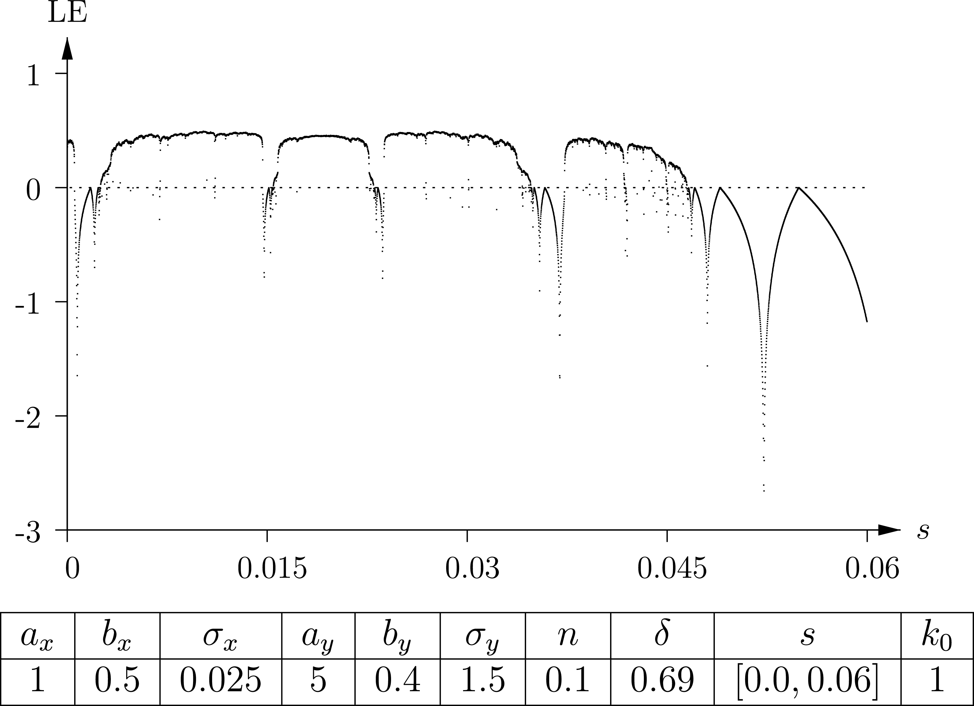
In many cases, however, only the period-3 cycle is numerically detected, because the other patterns exist only for a set of initial values of Lebesgue-measure zero. In contrast to topological chaos, numerical evidence for observable chaos is easier to detect. A model is said to exhibit observable chaos if a so-called strange attractor is observed, for example, see Onozaki et al. (Reference Onozaki, Sieg and Yokoo2000). 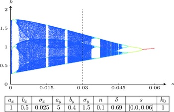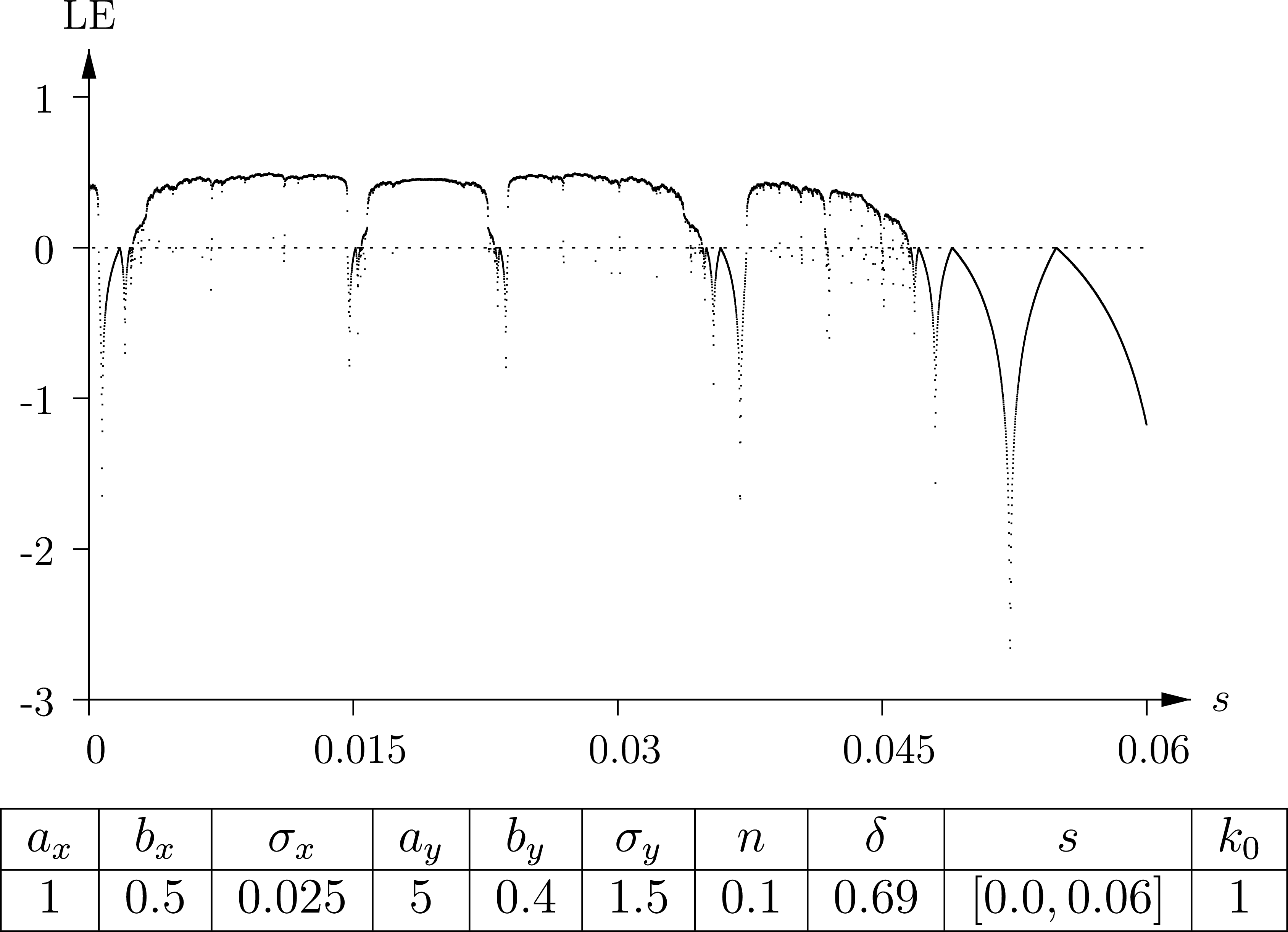These are numerically detected by computing Lyapunov exponents.Footnote ⁷ A positive Lyapunov exponent implies that the growth of capital-to-labour ratios depends sensitively on the initial capital-to-labour ratio. An attractor with such a property is called strange attractor. The bifurcation diagram in Figure 6 indicates that the savings propensity $s$ has to be very small in order for strange attractors to exist. The Lyapunov exponents of the corresponding growth paths over the same range of savings propensities are depicted in Figure 7. The diagrams lead the the conjecture that savings propensities above $5.5\%$ yield stable states, which confirms Lemma3 and our earlier analysis in Example5.

Figure 7.

Case A. Lyapunov exponents.

Figure 8.

Case B. Bifurcation diagramm over $b_y\in [0.01,0.09]$ .

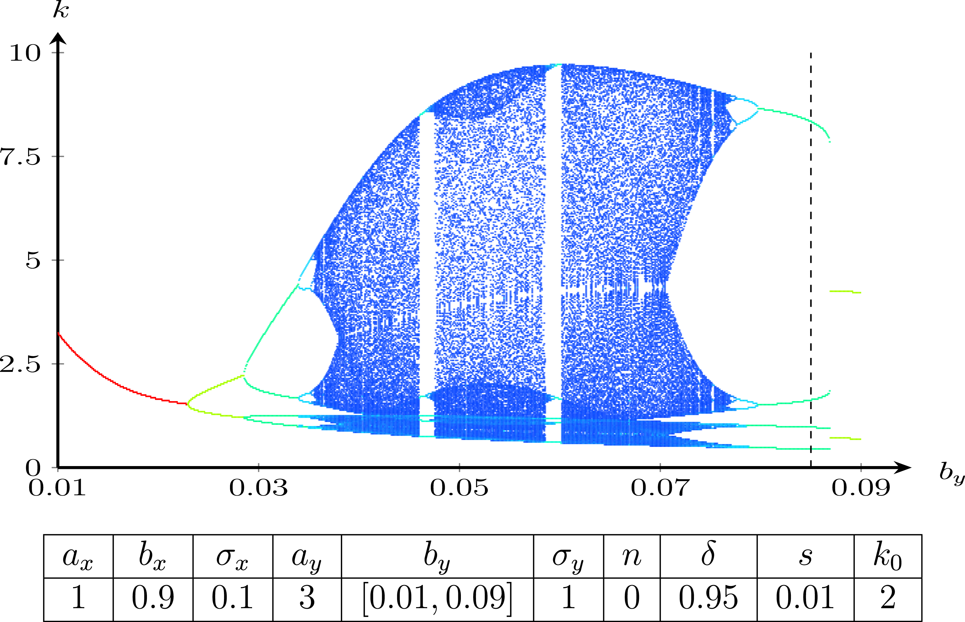
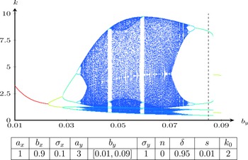
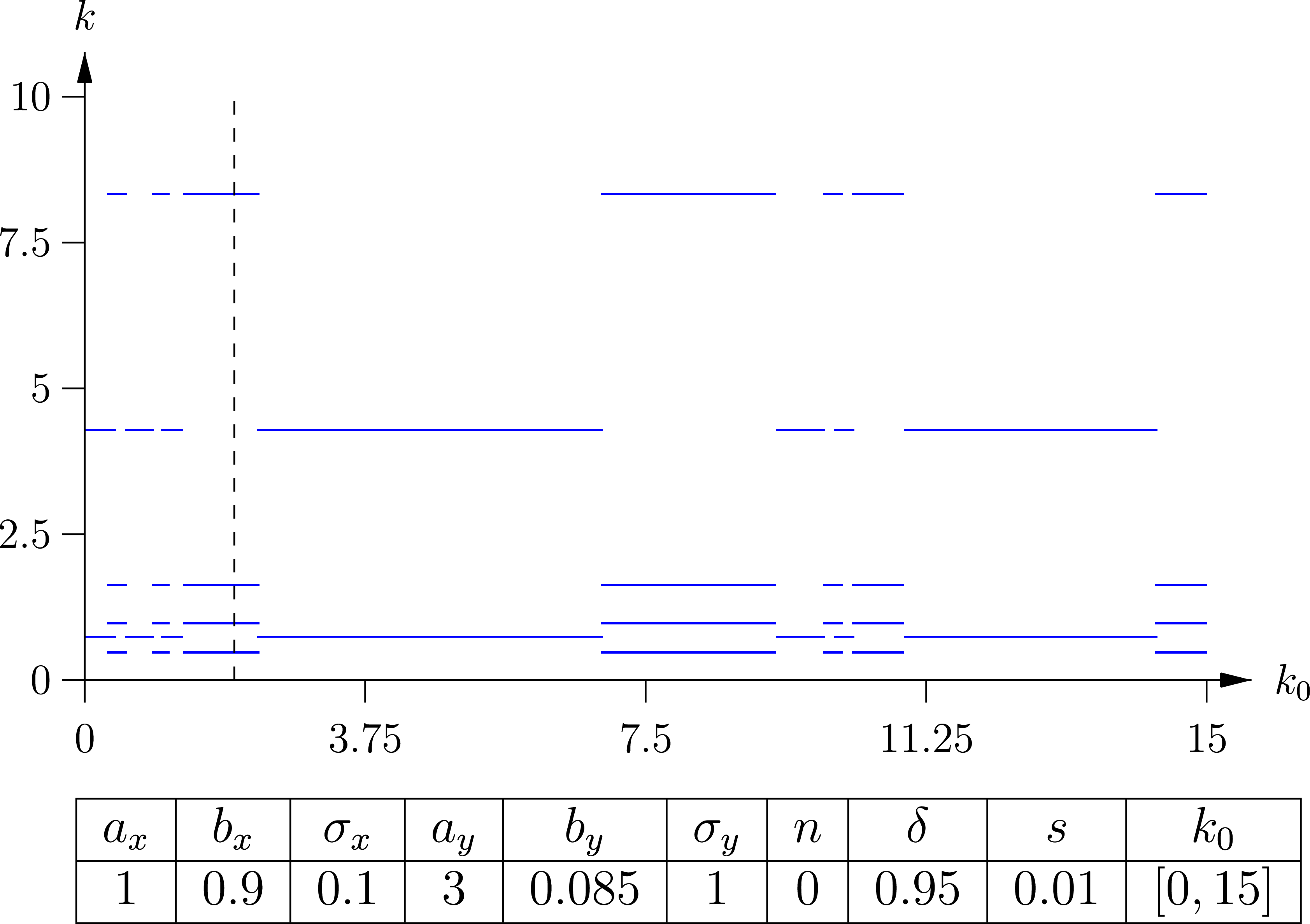
In view of Lemma5, the time-one map for case B depicted in Figure 2b has two steady states, a unique positive steady state and the origin. The dashed vertical line in the bifurcation diagram in Figure 8 shows that a period-4 cycle obtains for $b_y=0.085$ , indicating that both steady states may be unstable. This bifurcation diagram provides numerical evidence for topological chaos whenever the income distribution parameter $b_y$ assumes values, for example, in the neighbourhood of $0.05$ .Footnote ⁸

Figure 9.

Case B. Dependence on initial conditions $k_0\in [0,15]$ .

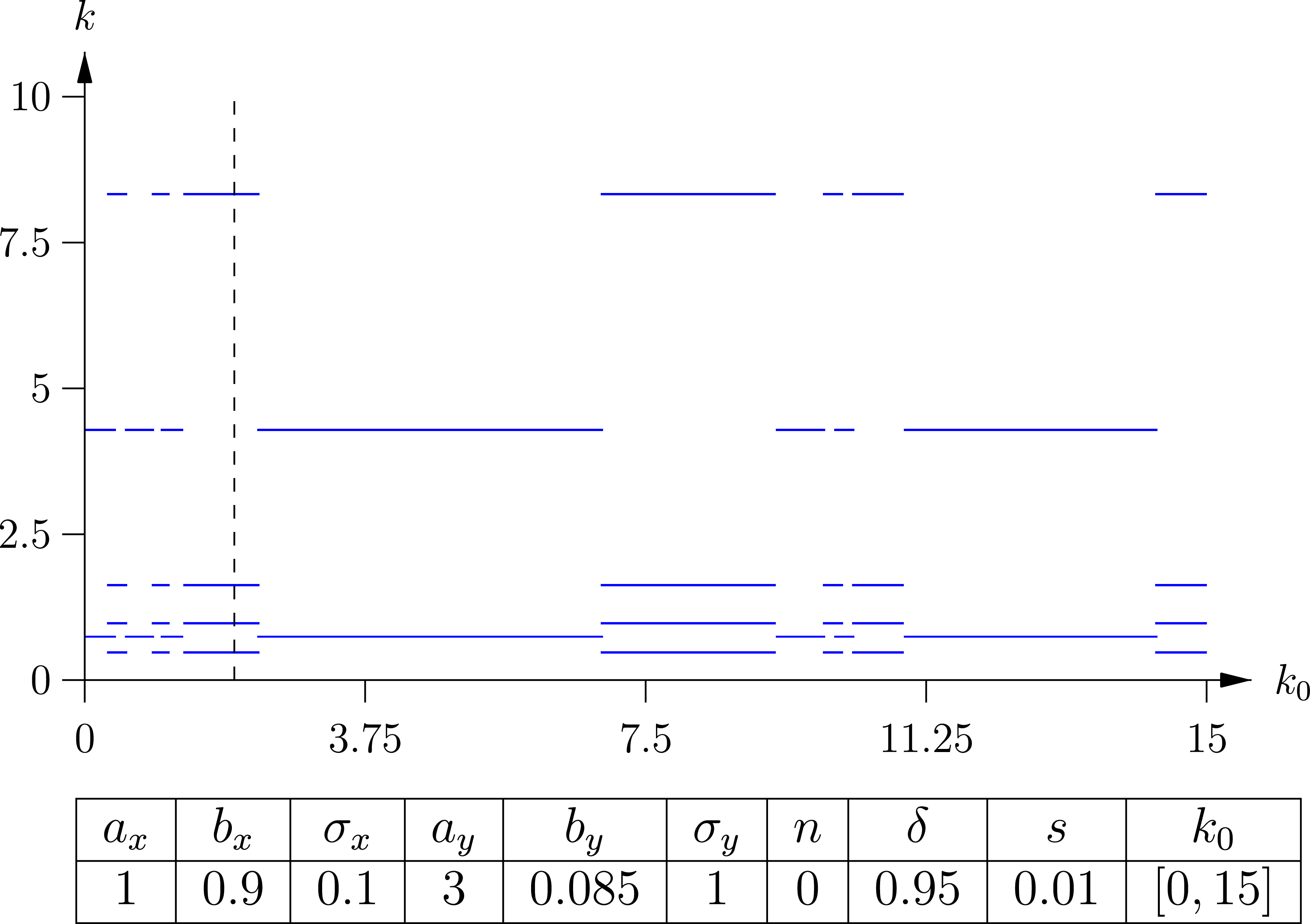
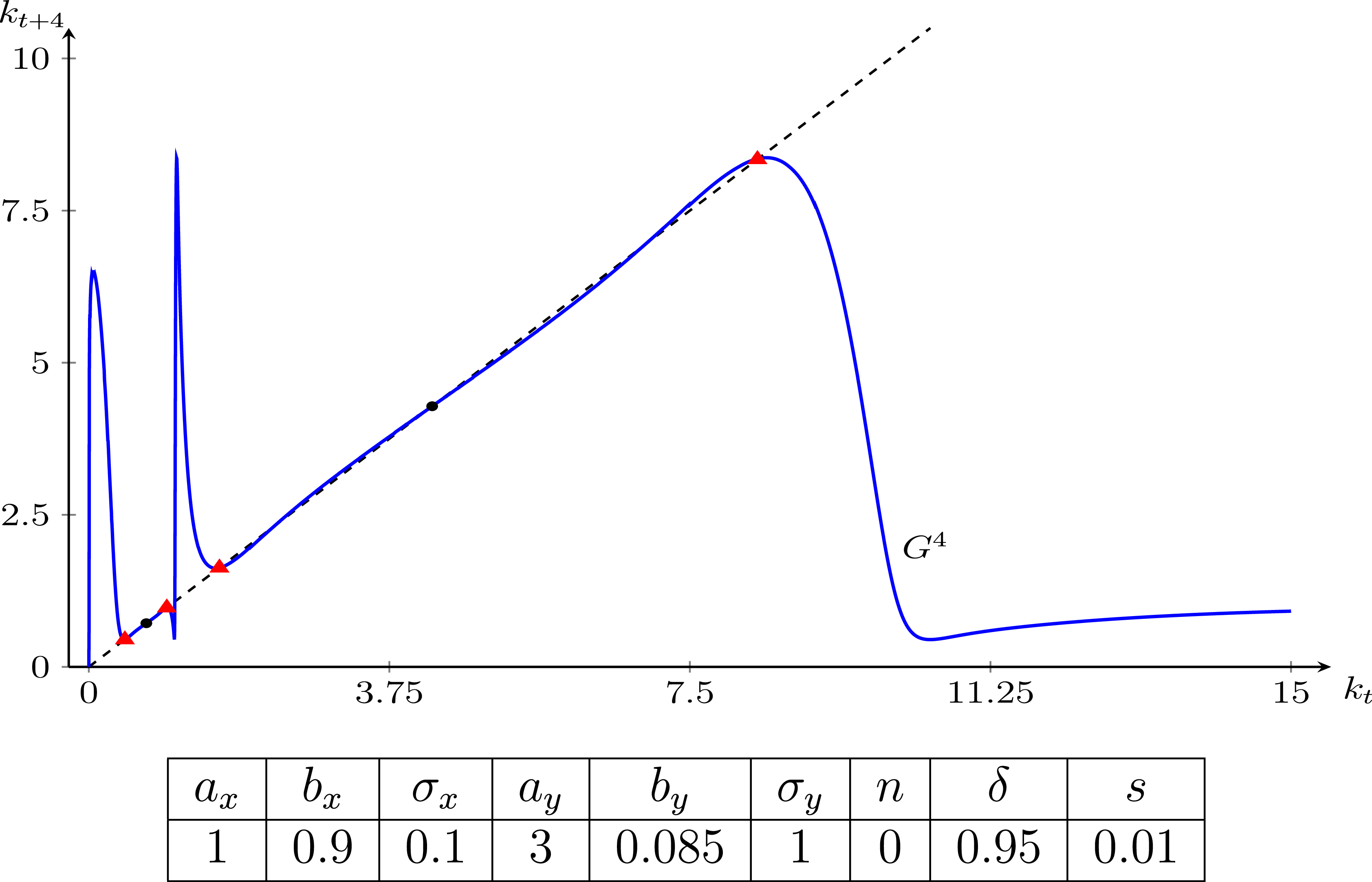
Figure 9 provides numerical evidence for the dependence on initial conditions. For initial capital-to-labour ratios $k_0$ ranging from $0$ to $15$ , the corresponding growth paths either converge to a period-2 cycle or to a period-4 cycle. The shape of the fourth iterate $G^4$ of the time-one map $G$ portrayed in Figure 10 provides some more insight into this phenomenon. A subcritical pitchfork bifurcation occurs when increasing the parameter $b_y$ from $0.08$ to $0.09$ . The period-2 cycle indicated by two dots, which already exists for $b_y=0.08$ , becomes asymptotically stable. Decreasing $b_y$ from $0.09$ to $0.08$ , an asymptotically stable period-4 cycle, marked by four triangles, emerges in addition to the existing period-2 cycle via a saddle-node bifurcation.

Figure 10.

Case B. Fourth iterate of $G$ .