


1. Introduction
In high-density environments, such as clusters of galaxies, gas stripping plays a crucial role in the evolution of constituent galaxies (Boselli & Gavazzi Reference Boselli and Gavazzi2006; Cortese, Catinella, & Smith Reference Cortese, Catinella and Smith2021). One such mechanism is ram pressure stripping (RPS; Gunn & Gott Reference Gunn1972). As the galaxy moves through the cluster, the hot ( $\mathrm{T} \sim 10^{7-8}\,\mathrm{K}$
), diffuse (
$\mathrm{T} \sim 10^{7-8}\,\mathrm{K}$
), diffuse ( $10^{-3}$
particles
$10^{-3}$
particles $\textrm{cm}^{-3}$
) intracluster medium (ICM) is able to remove the gas component of infalling galaxies by ram pressure (Gunn & Gott Reference Gunn1972). Ram pressure can remove the hot halo gas, leading to a gradual decline in star-formation over long timescales (strangulation; Larson, Tinsley, & Caldwell Reference Larson, Tinsley and Caldwell1980) or rapidly through stronger RPS that even evaporates the cold gas in the disc (Roediger & Brüggen Reference Roediger and Brüggen2006; Kapferer et al. Reference Kapferer, Sluka, Schindler, Ferrari and Ziegler2009).
$\textrm{cm}^{-3}$
) intracluster medium (ICM) is able to remove the gas component of infalling galaxies by ram pressure (Gunn & Gott Reference Gunn1972). Ram pressure can remove the hot halo gas, leading to a gradual decline in star-formation over long timescales (strangulation; Larson, Tinsley, & Caldwell Reference Larson, Tinsley and Caldwell1980) or rapidly through stronger RPS that even evaporates the cold gas in the disc (Roediger & Brüggen Reference Roediger and Brüggen2006; Kapferer et al. Reference Kapferer, Sluka, Schindler, Ferrari and Ziegler2009).
The signatures of ram pressure stripping manifest themselves through truncated discs, extra-planar emission, and one-sided spatial tails visible across the electromagnetic spectrum, in radio (Solanes et al. Reference Solanes2001; Vollmer et al. Reference Vollmer, Braine, Balkowski, Cayatte and Duschl2001; Chung et al. Reference Chung, van Gorkom, Kenney, Crowl and Vollmer2009; Yoon et al. Reference Yoon, Chung, Smith and Jaffé2017; Jáchym et al. Reference Jáchym2019; Roberts et al. Reference Roberts2021b), optical (narrow-band + broad-band) (Gavazzi et al. Reference Gavazzi2001; Koopmann & Kenney Reference Koopmann and Kenney2004; Cortese et al. Reference Cortese2007; Owers et al. Reference Owers, Couch, Nulsen and Randall2012; Abramson & Kenney Reference Abramson and Kenney2014; Ebeling, Stephenson, & Edge Reference Ebeling, Stephenson and Edge2014; Kenney et al. Reference Kenney2014; Poggianti et al. Reference Poggianti2016; Boselli et al. 2018; Owers et al. Reference Owers2019; Poggianti et al. Reference Poggianti2025), ultraviolet (Smith et al. Reference Smith2010; George et al. Reference George2018; George et al. Reference George2025), X-ray (Sun et al. Reference Sun2010; Poggianti et al. Reference Poggianti2019b).
The strength of these signatures ranges from mild to severe, and the presence and severity of these signatures are important indicators of the occurrence and degree of RPS. To identify the RPS candidates, studies typically adopt a bimodal approach, either by visual inspection of these features using multi-wavelength imaging (Smith et al. Reference Smith2010; Poggianti et al. Reference Poggianti2016; Yoon et al. Reference Yoon, Chung, Smith and Jaffé2017; Roberts & Parker Reference Roberts and Parker2020; Roberts et al. Reference Roberts2021b; Roberts et al. Reference Roberts2022b) or through structural measurements (McPartland et al. Reference McPartland, Ebeling, Roediger and Blumenthal2016; Roberts & Parker Reference Roberts and Parker2020; Roberts et al. Reference Roberts2021a; Roberts et al. Reference Roberts2022a; Bellhouse et al. Reference Bellhouse2022; Krabbe et al. Reference Krabbe2024). Focusing on the most extreme stripping cases – ‘jellyfish’ galaxies (Bekki Reference Bekki2009) where in situ star formation occurs in the stripped gas, forming star-forming tails that can extend up to several tens of kpc (Cortese et al. Reference Cortese2007; Sun et al. Reference Sun2010; Sheen et al. Reference Sheen2017; Poggianti et al. Reference Poggianti2019a) – Poggianti et al. (Reference Poggianti2016) classified 344 RPS candidates across 71 nearby clusters using B-band imaging and a visual classification scheme based on the degree of stripping (jellyfish class; JClass). Yoon et al. (Reference Yoon, Chung, Smith and Jaffé2017) applied a similar approach to classify HI morphologies of 35 galaxies in the Virgo cluster from the VLA Imaging of Virgo in Atomic Gas Survey (VIVA; Chung et al. Reference Chung, van Gorkom, Kenney, Crowl and Vollmer2009), while Roberts et al. (Reference Roberts2021b) exploited the Low-Frequency Array Two-metre Sky Survey (LoTSS; Shimwell et al. Reference Shimwell2019) radio continuum data to conduct a systematic search of RPS candidates, resulting in 95 galaxies with radio tails across 29 nearby clusters.
On the quantitative side, morphological parameters – for example, concentration (C), asymmetry (A), Gini coefficient (G), second-order moment of light ( $\mathrm{M}_{20}$
), Sérsic index (n), bulge strength parameter
$\mathrm{M}_{20}$
), Sérsic index (n), bulge strength parameter $F(G, {\mathrm{M}_{20}})$
– have been explored to identify RPS candidates. In such a study, McPartland et al. (Reference McPartland, Ebeling, Roediger and Blumenthal2016) used C, A, G,
$F(G, {\mathrm{M}_{20}})$
– have been explored to identify RPS candidates. In such a study, McPartland et al. (Reference McPartland, Ebeling, Roediger and Blumenthal2016) used C, A, G, $\mathrm{M}_{20}$
and skeletal decomposition (
$\mathrm{M}_{20}$
and skeletal decomposition ( $\mathrm{Sk}_{0-1}$
and
$\mathrm{Sk}_{0-1}$
and $\mathrm{Sk}_{1-2}$
) parameters to identify candidates at
$\mathrm{Sk}_{1-2}$
) parameters to identify candidates at ${z\sim0.5}$
using Hubble imaging through a semi-automated approach combining visual features and structural metrics. Krabbe et al. (Reference Krabbe2024) performed a similar analysis using Legacy Survey imaging for 600 galaxies across different environments, showing that strong jellyfish candidates (JClass
${z\sim0.5}$
using Hubble imaging through a semi-automated approach combining visual features and structural metrics. Krabbe et al. (Reference Krabbe2024) performed a similar analysis using Legacy Survey imaging for 600 galaxies across different environments, showing that strong jellyfish candidates (JClass $\gt$
3) can be distinguished from isolated galaxies through parameter combinations such as C–A, n–A, and F(G,
$\gt$
3) can be distinguished from isolated galaxies through parameter combinations such as C–A, n–A, and F(G, $\mathrm{M}_{20}$
)–A. All these findings show that galaxies with more extreme visual stripping evidence emerge as outliers in certain parameter spaces.
$\mathrm{M}_{20}$
)–A. All these findings show that galaxies with more extreme visual stripping evidence emerge as outliers in certain parameter spaces.
In terms of star formation, RPS-affected galaxies show a wide range of activity reported by both observations and simulations. Follow-up study on the Virgo spirals with truncated discs, Crowl & Kenney (Reference Crowl and Kenney2008) showed that stellar populations in the outer discs are consistent with being quenched within the last 0.5 Gyr. More recently, exploiting the spatially resolved data from the Sydney-AAO Multi-object Integral-field spectrograph (SAMI; Croom et al. Reference Croom2012) Galaxy Survey (SAMI-GS; Bryant et al. Reference Bryant2015), Owers et al. (Reference Owers2019) identified galaxies with strong H $\delta$
features (i.e. H
$\delta$
features (i.e. H $\delta$
-strong galaxies, HDSGs), as a tracer of recently quenched star formation and found that half of the cluster HDSGs (9/17) show ongoing star formation in their centres, supporting an outside-in quenching scenario. Simulations also demonstrate that RPS is able to rapidly quench star formation in a significant fraction of galaxies in group/cluster environments during the first pericentric passage, which is prominent for low-mass galaxies (Oman & Hudson Reference Oman and Hudson2016; Jung et al. Reference Jung2018; Lotz et al. Reference Lotz, Remus, Dolag, Biviano and Burkert2019; Rhee et al. Reference Rhee2024).
$\delta$
-strong galaxies, HDSGs), as a tracer of recently quenched star formation and found that half of the cluster HDSGs (9/17) show ongoing star formation in their centres, supporting an outside-in quenching scenario. Simulations also demonstrate that RPS is able to rapidly quench star formation in a significant fraction of galaxies in group/cluster environments during the first pericentric passage, which is prominent for low-mass galaxies (Oman & Hudson Reference Oman and Hudson2016; Jung et al. Reference Jung2018; Lotz et al. Reference Lotz, Remus, Dolag, Biviano and Burkert2019; Rhee et al. Reference Rhee2024).
Simulations indicate that RPS can also trigger an episode of intense star formation in both the disc and the stripped gas material by compression of giant molecular clouds (Bekki & Couch Reference Bekki and Couch2003) or ram-pressure-driven mass flows to the centre of the galaxy (Zhu, Tonnesen, & Bryan Reference Zhu, Tonnesen and Bryan2024). This may manifest as global and/or local elevated star formation activity. The global enhancement of star formation rates in jellyfish galaxies has been consistently reported by several observational studies (Vulcani et al. Reference Vulcani2018; Ebeling & Kalita Reference Ebeling and Kalita2019; Roman-Oliveira et al. Reference Roman-Oliveira2019; Roberts & Parker Reference Roberts and Parker2020; Roberts et al. Reference Roberts2021b; Lee et al. Reference Lee, Lee, Mun, Cho and Kang2022; Vulcani et al. Reference Vulcani2024), who found that jellyfish galaxies occupy the upper envelope of the star formation main sequence (SFMS).
With the emergence of integral field units, we are able to study the local/resolved ( $\lesssim$
1 kpc) properties of galaxies, such as star formation activity and metallicity, for a variety of galaxies with different morphologies, star formation stages, and even merger stages, particularly over the last decade (Ryder Reference Ryder1995; Sánchez et al. Reference Sánchez2013; Cano-Dìaz et al. Reference Cano-Dìaz2016; Hsieh et al. Reference Hsieh2017; Ellison et al. Reference Ellison2018; Medling et al. Reference Medling2018; Sánchez et al. Reference Sánchez2019; Thorp et al. Reference Thorp, Ellison, Simard, Sánchez and Antonio2019; Bluck et al. Reference Bluck2020a; Bluck et al. Reference Bluck2020b; Sánchez Reference Sánchez2020; Sánchez et al. Reference Sánchez2021; Mun et al. Reference Mun2024). This effort has been extended to understand the interplay between cluster environments and star formation activity through large campaigns such as the GAs Stripping Phenomena in galaxies with MUSE (GASP; Poggianti et al. Reference Poggianti2017). To that end, Vulcani et al. (Reference Vulcani2020) reported locally elevated star formation activity within the disc and stripped tails for the jellyfish galaxies identified within the GASP survey. A similar result of enhanced star formation activity has been found at the centre of a ram-pressure-affected galaxy by Zhu et al. (Reference Zhu, Tonnesen and Bryan2024) using tailored wind-tunnel simulations.
$\lesssim$
1 kpc) properties of galaxies, such as star formation activity and metallicity, for a variety of galaxies with different morphologies, star formation stages, and even merger stages, particularly over the last decade (Ryder Reference Ryder1995; Sánchez et al. Reference Sánchez2013; Cano-Dìaz et al. Reference Cano-Dìaz2016; Hsieh et al. Reference Hsieh2017; Ellison et al. Reference Ellison2018; Medling et al. Reference Medling2018; Sánchez et al. Reference Sánchez2019; Thorp et al. Reference Thorp, Ellison, Simard, Sánchez and Antonio2019; Bluck et al. Reference Bluck2020a; Bluck et al. Reference Bluck2020b; Sánchez Reference Sánchez2020; Sánchez et al. Reference Sánchez2021; Mun et al. Reference Mun2024). This effort has been extended to understand the interplay between cluster environments and star formation activity through large campaigns such as the GAs Stripping Phenomena in galaxies with MUSE (GASP; Poggianti et al. Reference Poggianti2017). To that end, Vulcani et al. (Reference Vulcani2020) reported locally elevated star formation activity within the disc and stripped tails for the jellyfish galaxies identified within the GASP survey. A similar result of enhanced star formation activity has been found at the centre of a ram-pressure-affected galaxy by Zhu et al. (Reference Zhu, Tonnesen and Bryan2024) using tailored wind-tunnel simulations.
While previous studies have predominantly focused on individual clusters or specific populations (e.g. jellyfish galaxies) to identify and examine stripping candidates, these approaches may not fully represent the broader quenching context. In particular, they may miss galaxies undergoing stripping without clear visible signatures. Therefore, homogeneous sampling of galaxies in clusters is essential. To achieve this, we use the SAMI-GS, which provides data for around 900 galaxies across clusters with diverse dynamical states, without any assumption on underlying galaxy population or feature-based selection (Owers et al. Reference Owers2017). Accordingly, this study is one of the few attempts to search for RPS candidates systematically without any pre-selection towards a certain galaxy population.
The outline of the paper is as follows. Section 2 describes the SAMI-GS, the data products used, whether existing or generated in this study. Section 3 introduces the visual classification scheme to identify the RPS candidates and investigates the positions in projected phase space and star-forming properties of galaxies in different visual classes. In Section 4, we discuss our findings and interpretation with respect to previous studies. Section 5 highlights the key findings of the study. Throughout this paper, we assume a flat $\Lambda$
CDM cosmology with
$\Lambda$
CDM cosmology with $\mathrm{H}_0 = 70\,\text{km}\,\text{s}^{-1}\,\text{Mpc}^{-1}$
,
$\mathrm{H}_0 = 70\,\text{km}\,\text{s}^{-1}\,\text{Mpc}^{-1}$
, $\Omega_{m} = 0.3, \ \Omega_\Lambda = 0.7$
.
$\Omega_{m} = 0.3, \ \Omega_\Lambda = 0.7$
.
2. Data and sample selection
2.1. SAMI Galaxy Survey
The SAMI-GS was carried out with the SAMI instrument mounted at the prime focus of the 3.9 m Anglo-Australian Telescope (AAT). The SAMI instrument uses 13 integral-field units (namely hexabundles; Bland-Hawthorn et al. Reference Bland-Hawthorn2011; Bryant et al. Reference Bryant, Bland-Hawthorn, Fogarty, Lawrence and Croom2014) composed of 61 fused 1.6 arcsec-diameter fibres. These hexabundles are fed into the AAOmega spectrograph (Sharp et al. Reference Sharp, McLean and Iye2006). As of SAMI Data Release 3 (DR3; Croom et al. Reference Croom2021), the SAMI-GS observed 3 068 unique galaxies sampled from the Galaxy and Mass Assembly Survey (GAMA; Driver et al. Reference Driver2011) equatorial regions (G09, G12, G15; 2151 galaxies) and eight cluster regions selected from the catalogue of De Propris et al. (Reference De Propris2002) in the 2-degree Field Galaxy Redshift Survey, and the Cluster Infall Regions in the Sloan Digital Sky Survey (CIRS; Rines & Diaferio Reference Rines and Diaferio2006), with halo masses of ${14.25\leq \log\left(\mathrm{M}_{200}/\mathrm{M}_\odot\right)\leq 15.19}$
(917 galaxies) described in Owers et al. (Reference Owers2017). The observed galaxies have stellar masses ranging between
${14.25\leq \log\left(\mathrm{M}_{200}/\mathrm{M}_\odot\right)\leq 15.19}$
(917 galaxies) described in Owers et al. (Reference Owers2017). The observed galaxies have stellar masses ranging between $8\lt$ ${\log\left(\mathrm{M}_{*}/\mathrm{M}_\odot\right)}$ $\lt 12$
.
$\lt 12$
.
The details for target selection are given in Bryant et al. (Reference Bryant2015) for GAMA regions and Owers et al. (Reference Owers2017) for the cluster sample. Briefly, the primary targets are selected with a step-like stellar mass function with an increasing lower limit as a function of redshift, where redshift refers to the flow-corrected value, $z_{\text{tonry}}$
, for the GAMA regions (Tonry et al. Reference Tonry, Blakeslee, Ajhar and Dressler2000; Baldry et al. Reference Baldry2012). To define primary targets for the cluster regions, only two steps are adopted as
$z_{\text{tonry}}$
, for the GAMA regions (Tonry et al. Reference Tonry, Blakeslee, Ajhar and Dressler2000; Baldry et al. Reference Baldry2012). To define primary targets for the cluster regions, only two steps are adopted as ${\log\left(\mathrm{M}_{*}/\mathrm{M}_\odot\right)}$ $\gt$
9.5 if the cluster redshift,
$\gt$
9.5 if the cluster redshift, $ z_{cl},\lt 0.045$
, otherwise
$ z_{cl},\lt 0.045$
, otherwise ${\log\left(\mathrm{M}_{*}/\mathrm{M}_\odot\right)}$ $\gt$
10. Additionally, cluster targets are selected within
$\gt$
10. Additionally, cluster targets are selected within ${R}_{200}$
and
${R}_{200}$
and $|v_{\text{pec}}|/\sigma_{200}\leq3.5$
, where
$|v_{\text{pec}}|/\sigma_{200}\leq3.5$
, where $v_{\text{pec}}$
is the peculiar velocity of galaxies with respect to the cluster redshift,
$v_{\text{pec}}$
is the peculiar velocity of galaxies with respect to the cluster redshift, $v_{\text{pec}} = c \times (z_{\text{gal}} - z_{\text{cl}}) / (1 + z_{cl}$
) with c being the speed of light, and
$v_{\text{pec}} = c \times (z_{\text{gal}} - z_{\text{cl}}) / (1 + z_{cl}$
) with c being the speed of light, and $\sigma_{200}$
is the velocity dispersion of the cluster measured within
$\sigma_{200}$
is the velocity dispersion of the cluster measured within ${R}_{200}$
defined by Owers et al. (Reference Owers2017). Note that both
${R}_{200}$
defined by Owers et al. (Reference Owers2017). Note that both $z_{\text{cl}}$
and
$z_{\text{cl}}$
and $z_{\text{gal}}$
are not flow-corrected. This selection is less strict than the cluster membership allocation done by Owers et al. (Reference Owers2017), which was based on caustic analysis, and it therefore includes non-bona fide members with redshifts close to the cluster.
$z_{\text{gal}}$
are not flow-corrected. This selection is less strict than the cluster membership allocation done by Owers et al. (Reference Owers2017), which was based on caustic analysis, and it therefore includes non-bona fide members with redshifts close to the cluster.
One of the main aims of this study is to understand the environmental impact on star formation activity. To achieve this, we need a sample from a non-cluster field as a reference/control. Therefore, we use the GAMA portion of the survey as a control sample, which will enable a direct comparison to assess environmental effects. GAMA galaxies are selected through a step-like stellar mass function for $ 0.005 \lt z_{\text{tonry}} \lt 0.095$
(Bryant et al. Reference Bryant2015), which is shown in Figure 2.
$ 0.005 \lt z_{\text{tonry}} \lt 0.095$
(Bryant et al. Reference Bryant2015), which is shown in Figure 2.
2.2. SAMI data products
2.2.1. Emission line measurements
The emission line fitting procedure is outlined in Green et al. (Reference Green2018), Scott et al. (Reference Scott2018), Croom et al. (Reference Croom2021). Briefly, strong emission lines (i.e. [OII] $(\lambda\lambda3726,3729)$
, H
$(\lambda\lambda3726,3729)$
, H $\beta$
, [OIII]
$\beta$
, [OIII] $\lambda5007$
, H
$\lambda5007$
, H $\alpha$
, [NII]
$\alpha$
, [NII] $\lambda$
6584, [SII]
$\lambda$
6584, [SII] $(\lambda\lambda6716, 6731)$
) are simultaneously fitted by Lzifu (Ho et al. Reference Ho2016) per spaxel. The underlying stellar continuum is modelled and subtracted following Owers et al. (Reference Owers2019). Based on the redshifts from the SAMI input catalogues (Bryant et al. Reference Bryant2015; Owers et al. Reference Owers2017), Lzifu then fits up to three Gaussian components to the emission lines, assuming the same gas kinematics across lines. Note that this component analysis is only applied to H
$(\lambda\lambda6716, 6731)$
) are simultaneously fitted by Lzifu (Ho et al. Reference Ho2016) per spaxel. The underlying stellar continuum is modelled and subtracted following Owers et al. (Reference Owers2019). Based on the redshifts from the SAMI input catalogues (Bryant et al. Reference Bryant2015; Owers et al. Reference Owers2017), Lzifu then fits up to three Gaussian components to the emission lines, assuming the same gas kinematics across lines. Note that this component analysis is only applied to H $\alpha$
since it usually has a higher SNR relative to other lines. In this paper, we use the total flux of H
$\alpha$
since it usually has a higher SNR relative to other lines. In this paper, we use the total flux of H $\alpha$
along with H
$\alpha$
along with H $\beta$
, [OIII]
$\beta$
, [OIII] $\lambda5007$
, and [NII]
$\lambda5007$
, and [NII] $\lambda6584$
lines.
$\lambda6584$
lines.
2.2.2. Spectral classification maps
We adopt the spectral classification scheme described in Owers et al. (Reference Owers2019). The scheme incorporates the emission and absorption line features simultaneously. A spectrum is classified as ‘emission’ if a spaxel exhibits either H $\alpha$
or [NII]
$\alpha$
or [NII] $\lambda$
6584 (i.e. the primary lines) and an additional line from H
$\lambda$
6584 (i.e. the primary lines) and an additional line from H $\beta$
, [OIII]
$\beta$
, [OIII] $\lambda$
5007 [SII]
$\lambda$
5007 [SII] $\lambda6716$
, or [SII]
$\lambda6716$
, or [SII] $\lambda6731$
with SNR=(flux/
$\lambda6731$
with SNR=(flux/ $\sigma_{\text{flux}})\gt 3$
, where
$\sigma_{\text{flux}})\gt 3$
, where $\sigma_{\text{flux}}$
is the associated flux uncertainty estimated through a least-square fitting procedure (Ho et al. Reference Ho2016). To avoid spurious detections due to template mismatches, the primary line must also have equivalent width, EW
$\sigma_{\text{flux}}$
is the associated flux uncertainty estimated through a least-square fitting procedure (Ho et al. Reference Ho2016). To avoid spurious detections due to template mismatches, the primary line must also have equivalent width, EW $\gt$
1 Å. Otherwise, the spectrum is classified as ‘absorption’.
$\gt$
1 Å. Otherwise, the spectrum is classified as ‘absorption’.
The emission line classification of Owers et al. (Reference Owers2019) is summarised as follows:
-
• If H $\alpha$
, [NII]
$\lambda$
6584, and at least one of H
$\beta$
or [OIII]
$\lambda$
5007 are detected, Baldwin, Phillips & Terlevich (BPT) diagnostic (Baldwin, Phillips, & Terlevich Reference Baldwin, Phillips and Terlevich1981) is applied to classify the ionisation source as ‘star-forming (SF)’, or ‘intermediate (INT)’, or ‘non-star-forming (NSF)’, through the demarcation lines defined by Kewley et al. (Reference Kewley, Dopita, Sutherland, Heisler and Trevena2001) (Ke01) and Kauffmann et al. (Reference Kauffmann2003) (Ka03).
$\alpha$
, [NII]
$\lambda$
6584, and at least one of H
$\beta$
or [OIII]
$\lambda$
5007 are detected, Baldwin, Phillips & Terlevich (BPT) diagnostic (Baldwin, Phillips, & Terlevich Reference Baldwin, Phillips and Terlevich1981) is applied to classify the ionisation source as ‘star-forming (SF)’, or ‘intermediate (INT)’, or ‘non-star-forming (NSF)’, through the demarcation lines defined by Kewley et al. (Reference Kewley, Dopita, Sutherland, Heisler and Trevena2001) (Ke01) and Kauffmann et al. (Reference Kauffmann2003) (Ka03). -
• If only H
$\alpha$
and [NII]
$\lambda$
6584 are present, WHAN diagram of Cid Fernandes et al. (Reference Cid Fernandes2010) is used. SF, INT, and NSF classes are separated using
$\log$
([NII]
$\lambda 6584/H\alpha$
) =
$-0.32$
and
$\log$
([NII]
$\lambda6584/H\alpha$
) =
$-0.1$
values, which approximate the Ke01 and Ke03 demarcation lines, respectively. -
• In case of one of the primary lines missing, the classification is done as follows – star-forming (SF) if H
$\alpha$
is present, and non-SF if only [NII]
$\lambda$
6584 is detected. -
• Additional sub-classes are defined based on the H
$\alpha$
line strength, following the recipe given in Cid Fernandes et al. (Reference Cid Fernandes2010). If EW(H
$\alpha$
)
$\lt$
3 Å, the spectrum can be divided into ‘wSF’ or ‘rINT’ or ‘rNSF’. NSF spectra with EW(H
$\alpha$
) ranging between 3 and 6 Å are classified as ‘wNSF’, whereas those with EW(H
$\alpha$
)
$\gt$
6 Å are ‘sNSF’. Here, ‘r’, ‘w’, and ‘s’ stand for ‘retired’, ‘weak’, and ‘strong’ sub-classes defined by Cid Fernandes et al. (Reference Cid Fernandes2010).


Absorption line measurements are carried out on absorption spectra as well as on emission spectra classified as NSF spectra, whose emission is not powered by photoionisation. The spectra with strong Balmer absorption (i.e. EW $(\overline{\mathrm{H}_{\delta\gamma\beta}})\lt -3$
Å and
$(\overline{\mathrm{H}_{\delta\gamma\beta}})\lt -3$
Å and $|\mathrm{SNR}(\mathrm{EW}(\overline{\mathrm{H}_{\delta\gamma\beta}}))|\gt 3$
) are classified as ‘H
$|\mathrm{SNR}(\mathrm{EW}(\overline{\mathrm{H}_{\delta\gamma\beta}}))|\gt 3$
) are classified as ‘H $\delta$
-strong (HDS)’ or ‘non-star-forming H
$\delta$
-strong (HDS)’ or ‘non-star-forming H $\delta$
-strong (NSF-HDS)’. The absorption spectra not exhibiting strong Balmer absorption are categorised as ‘passive’.
$\delta$
-strong (NSF-HDS)’. The absorption spectra not exhibiting strong Balmer absorption are categorised as ‘passive’.
Combining emission and absorption classification, the global spectroscopic classification is performed as follows: ‘passive galaxies (PASGs)’ are defined as with more than 90% of the spaxels classified as ‘passive’, ‘rNSF’, ‘rINT’, ‘wNSF’, ‘sNSF’, or ‘wSF’; ‘star-forming galaxies (SFGs)’ are those present with at least 10% of the spaxels as ‘SF’ or ‘INT’; galaxies, where ‘HDS’ or ‘NSF-HDS’ spaxels are making up more than 10% of the total, are classified as ‘H $\delta$
-strong galaxies (HDSGs)’. Please refer to Owers et al. (Reference Owers2019) for the complete procedure of spectroscopic classification.
$\delta$
-strong galaxies (HDSGs)’. Please refer to Owers et al. (Reference Owers2019) for the complete procedure of spectroscopic classification.
A visualisation of the steps involved in producing the ionised gas map for an example galaxy, 9011900084. The two leftmost panels show the H $\alpha$
and [NII]
$\alpha$
and [NII] $\lambda$
6584 flux maps generated using the detection procedure described in Section 2.2.2, and the colour bar presents the flux values. The middle panel presents the final emission detection map, highlighting connected spaxels and coloured by the detected emission line, which is also shown in the colour bar. The two rightmost panels show the total emission map, derived from the final detection map using the same colour bar as the leftmost panels but applied to H
$\lambda$
6584 flux maps generated using the detection procedure described in Section 2.2.2, and the colour bar presents the flux values. The middle panel presents the final emission detection map, highlighting connected spaxels and coloured by the detected emission line, which is also shown in the colour bar. The two rightmost panels show the total emission map, derived from the final detection map using the same colour bar as the leftmost panels but applied to H $\alpha$
+ [NII]
$\alpha$
+ [NII] $\lambda$
6584 emission. The corresponding binary detection map is also shown, where ‘1’ and ‘0’ indicate spaxels with and without detected emission, respectively. The black and red contours displayed in all panels refer to the stellar continuum defined in Section 3.1, and the SAMI field of view, respectively. The orientation is as North towards up, and East towards the left.
$\lambda$
6584 emission. The corresponding binary detection map is also shown, where ‘1’ and ‘0’ indicate spaxels with and without detected emission, respectively. The black and red contours displayed in all panels refer to the stellar continuum defined in Section 3.1, and the SAMI field of view, respectively. The orientation is as North towards up, and East towards the left.

2.2.3. Ionised gas maps
The primary goal of the paper is to identify galaxies with signatures of ongoing or recent ram pressure stripping and study their properties. Since it is well-established that RPS acts on the gas component (Boselli & Gavazzi Reference Boselli and Gavazzi2006; Cortese et al. Reference Cortese, Catinella and Smith2021), we therefore need to define the ionised gas distribution. The origin of the ionisation might be due to either recently formed stars (SF), as observed in jellyfish galaxies (Poggianti et al. Reference Poggianti2019a), or non-star-forming (NSF) ionisation (Fossati et al. Reference Fossati2016; Pedrini et al. 2022). To account for both SF and NSF ionisation, we produce the ionised gas maps by combining H $\alpha$
+[NII]
$\alpha$
+[NII] $\lambda$
6584 emission that will be used to characterise the morphological parameters of the gas distribution.
$\lambda$
6584 emission that will be used to characterise the morphological parameters of the gas distribution.
We determine the spaxels with reliable emission measurements by running a per-spaxel detection filter, which applies a set of criteria to exclude bad spaxels. The main criteria on emission line properties are the same as those outlined in Owers et al. (Reference Owers2019) to define emission spectra (also summarised in Section 2.2.2). Additional criteria spaxel selection criteria are: ${|v_{\text{gas}}|}\ \& \ \sigma_{\mathrm{gas}} \lt 500 \mathrm{\ km\ s^{-1}}$
, and their associated uncertainties must be less than 30 km
${|v_{\text{gas}}|}\ \& \ \sigma_{\mathrm{gas}} \lt 500 \mathrm{\ km\ s^{-1}}$
, and their associated uncertainties must be less than 30 km $s^{-1}$
, ensuring the reliable emission fits are being used.
$s^{-1}$
, ensuring the reliable emission fits are being used.
The final step combines the H $\alpha$
and [NII]
$\alpha$
and [NII] $\lambda$
6584 maps while enforcing an 8-connectivity rule and requires a spaxel with either H
$\lambda$
6584 maps while enforcing an 8-connectivity rule and requires a spaxel with either H $\alpha$
or [NII]
$\alpha$
or [NII] $\lambda$
6584 detection to have at least three neighbouring detections. This ensures spatial coherence and excludes isolated low-SNR spaxels and/or high-SNR spurious detection.
$\lambda$
6584 detection to have at least three neighbouring detections. This ensures spatial coherence and excludes isolated low-SNR spaxels and/or high-SNR spurious detection.
Once the final detection map is produced, for the spaxels with detections of both H $\alpha$
and [NII]
$\alpha$
and [NII] $\lambda$
6584, we sum fluxes (i.e. H
$\lambda$
6584, we sum fluxes (i.e. H $\alpha$
+ [NII]
$\alpha$
+ [NII] $\lambda$
6584) and propagate the uncertainties (i.e.
$\lambda$
6584) and propagate the uncertainties (i.e. $\sqrt{\sigma_{H\alpha}^2 + \sigma_{\text{NII}}^2}$
); otherwise, we keep the flux and uncertainty as they are. Based on this final detection map, we also generate a binary detection map, in which ‘1’ is assigned if there is a detection and ‘0’ if none. Figure 1 illustrates the products resulting from each step of the detection procedure.
$\sqrt{\sigma_{H\alpha}^2 + \sigma_{\text{NII}}^2}$
); otherwise, we keep the flux and uncertainty as they are. Based on this final detection map, we also generate a binary detection map, in which ‘1’ is assigned if there is a detection and ‘0’ if none. Figure 1 illustrates the products resulting from each step of the detection procedure.
2.2.4. SFR maps
One key element of this study is to understand how RPS influences star-formation activity. Using IFU observations from SAMI, we are able to conduct a spatially resolved examination of star-forming properties of cluster galaxies. In this section, we describe the procedure to generate resolved SFR maps estimated from H $\alpha$
fluxes.
$\alpha$
fluxes.
We make use of the per-spaxel classification scheme of Owers et al. (Reference Owers2019) to identify star-forming spaxels. For these star-forming spaxels, we correct H $\alpha$
fluxes for intrinsic dust extinction and Galactic foreground extinction similar to the recipes given in Medling et al. (Reference Medling2018) and Mun et al. (Reference Mun2024). The dust extinction is corrected using the observed Balmer decrement (BD),
$\alpha$
fluxes for intrinsic dust extinction and Galactic foreground extinction similar to the recipes given in Medling et al. (Reference Medling2018) and Mun et al. (Reference Mun2024). The dust extinction is corrected using the observed Balmer decrement (BD), $(\mathrm{H}\alpha/\mathrm{H}\beta)_\mathrm{{obs}}$
. Here, BD maps are smoothed by a truncated Gaussian kernel with FWHM of 1.6 spaxels in order to account for aliasing in the differential atmospheric refraction effect (refer to Medling et al. Reference Medling2018 for details). We assume an intrinsic BD,
$(\mathrm{H}\alpha/\mathrm{H}\beta)_\mathrm{{obs}}$
. Here, BD maps are smoothed by a truncated Gaussian kernel with FWHM of 1.6 spaxels in order to account for aliasing in the differential atmospheric refraction effect (refer to Medling et al. Reference Medling2018 for details). We assume an intrinsic BD, $(\mathrm{H}\alpha/\mathrm{H}\beta)_\mathrm{{int}}$
, value of 2.86 based on Case B recombination line (Osterbrock Reference Osterbrock1989; Calzetti et al. Reference Calzetti2000), and Milky Way extinction curve (i.e.
$(\mathrm{H}\alpha/\mathrm{H}\beta)_\mathrm{{int}}$
, value of 2.86 based on Case B recombination line (Osterbrock Reference Osterbrock1989; Calzetti et al. Reference Calzetti2000), and Milky Way extinction curve (i.e. $R_V \simeq 3.1$
) from Cardelli et al. (Reference Cardelli, Clayton and Mathis1989). For spaxels without H
$R_V \simeq 3.1$
) from Cardelli et al. (Reference Cardelli, Clayton and Mathis1989). For spaxels without H $\beta$
detection, or with observed BD less than intrinsic value (i.e. 2.86), we fix the correction value and its error to 1 and 0, respectively, by following Medling et al. (Reference Medling2018). Additionally,Footnote
a
the spaxels with observed BD greater than 10, or H
$\beta$
detection, or with observed BD less than intrinsic value (i.e. 2.86), we fix the correction value and its error to 1 and 0, respectively, by following Medling et al. (Reference Medling2018). Additionally,Footnote
a
the spaxels with observed BD greater than 10, or H $\alpha$
flux
$\alpha$
flux $\gt 40\times 10^{-16}\ \mathrm{erg/s/cm^{-2}}$
are excluded, to eliminate spurious H
$\gt 40\times 10^{-16}\ \mathrm{erg/s/cm^{-2}}$
are excluded, to eliminate spurious H $\alpha$
fits to the edges of the bundles. The foreground Galactic extinction is corrected for H
$\alpha$
fits to the edges of the bundles. The foreground Galactic extinction is corrected for H $\alpha$
fluxes using dust maps produced by Schlegel et al. (Reference Schlegel, Finkbeiner and Davis1998), Schlafly & Finkbeiner (Reference Schlafly and Finkbeiner2011) for the given coordinates. We use the observed frame wavelengths to obtain the extinction coefficients.
$\alpha$
fluxes using dust maps produced by Schlegel et al. (Reference Schlegel, Finkbeiner and Davis1998), Schlafly & Finkbeiner (Reference Schlafly and Finkbeiner2011) for the given coordinates. We use the observed frame wavelengths to obtain the extinction coefficients.
Once extinction-corrected H $\alpha$
fluxes are obtained, we convert them to H
$\alpha$
fluxes are obtained, we convert them to H $\alpha$
luminosities via luminosity distances for the adopted cosmology. The redshifts of cluster galaxies are fixed to the cluster redshift to minimise the scatter due to peculiar motions relative to the cosmological redshift of the cluster, while
$\alpha$
luminosities via luminosity distances for the adopted cosmology. The redshifts of cluster galaxies are fixed to the cluster redshift to minimise the scatter due to peculiar motions relative to the cosmological redshift of the cluster, while $z_{\text{tonry}}$
values (Baldry et al. Reference Baldry2012; Bryant et al. Reference Bryant2015) are used for the GAMA sample. We then determine SFRs by implementing the estimator given by Kennicutt (Reference Kennicutt1998) as follows:
$z_{\text{tonry}}$
values (Baldry et al. Reference Baldry2012; Bryant et al. Reference Bryant2015) are used for the GAMA sample. We then determine SFRs by implementing the estimator given by Kennicutt (Reference Kennicutt1998) as follows:
 \begin{equation} SFR = \frac{7.92 \times 10^{-42} \times L_{H\alpha}}{1.53} \ \ [\mathrm{M_\odot \ yr^{-1}}]\end{equation}
Here, $L_{H\alpha}$
is H
$L_{H\alpha}$
is H $\alpha$
luminosity, and 1.53 is the conversion factor between the Salpeter (Reference Salpeter1955) and Chabrier (Reference Chabrier2003) initial mass functions.
$\alpha$
luminosity, and 1.53 is the conversion factor between the Salpeter (Reference Salpeter1955) and Chabrier (Reference Chabrier2003) initial mass functions.
For the given redshift range, a spaxel covers a range of physical size in kpc. Therefore, to compare SFRs within the same physical size, we determine star formation surface densities, $\Sigma_{\mathrm{SFR}}$
, by normalising SFR with the physical area of each spaxel as follows:
$\Sigma_{\mathrm{SFR}}$
, by normalising SFR with the physical area of each spaxel as follows:
 \begin{equation} \Sigma_{SFR} = \frac{SFR}{(0.5 \times PS(z) )^2}\ \ [\mathrm{M_\odot \ yr^{-1} \ kpc^{-2}}]\end{equation}
where 0.5 is the SAMI pixel scale in arcsecond/spaxel and PS(z) is the physical size in kpc/arcsecond for the adopted cosmology. Redshifts are treated the same as above. Uncertainties are estimated by propagating the formal errors of H $\alpha$
and H
$\alpha$
and H $\beta$
fluxes using the uncertainties Python package (Lebigot Reference Lebigot2024).
$\beta$
fluxes using the uncertainties Python package (Lebigot Reference Lebigot2024).
Left panel: Stellar mass and redshift ( $z_{\text{tonry}}$
for GAMA) distribution of the full SAMI sample (Croom et al. Reference Croom2021) with available spectroscopic classification from Owers et al. (Reference Owers2019)
$z_{\text{tonry}}$
for GAMA) distribution of the full SAMI sample (Croom et al. Reference Croom2021) with available spectroscopic classification from Owers et al. (Reference Owers2019) $(N=2\,908)$
. The cyan and red points represent the primary targets for GAMA and cluster regions, respectively, whereas the green pluses and black crosses show the secondary targets for the same samples. The black solid line shows the selection steps in stellar mass for primary GAMA targets as defined in Bryant et al. (Reference Bryant2015). The black dashed line marks the lower stellar mass limit we adopted in this study –
$(N=2\,908)$
. The cyan and red points represent the primary targets for GAMA and cluster regions, respectively, whereas the green pluses and black crosses show the secondary targets for the same samples. The black solid line shows the selection steps in stellar mass for primary GAMA targets as defined in Bryant et al. (Reference Bryant2015). The black dashed line marks the lower stellar mass limit we adopted in this study – ${\log\left(\mathrm{M}_{*}/\mathrm{M}_\odot\right)}=10$
. The blue hatched area encloses GAMA galaxies selected as a control sample. Middle panel: The distribution of detection fraction (
${\log\left(\mathrm{M}_{*}/\mathrm{M}_\odot\right)}=10$
. The blue hatched area encloses GAMA galaxies selected as a control sample. Middle panel: The distribution of detection fraction ( $f_{\text{det}}$
) of cluster galaxies, as defined in Section 2.3, with
$f_{\text{det}}$
) of cluster galaxies, as defined in Section 2.3, with $N_{\text{spaxel}}(Emission) \neq 0 (N=194)$
. The red, blue, and green step histograms show the distributions for passive galaxies (PASGs), star-forming galaxies (SFGs), and H
$N_{\text{spaxel}}(Emission) \neq 0 (N=194)$
. The red, blue, and green step histograms show the distributions for passive galaxies (PASGs), star-forming galaxies (SFGs), and H $\delta$
-strong galaxies (HDSGs), respectively. The black vertical line marks the cut applied as
$\delta$
-strong galaxies (HDSGs), respectively. The black vertical line marks the cut applied as $f_{\text{det}} \gt 0.2$
. Right panel: The stellar mass distributions of the final cluster sample defined in Section 3.2
$f_{\text{det}} \gt 0.2$
. Right panel: The stellar mass distributions of the final cluster sample defined in Section 3.2 $(N=81)$
and the selected star-forming GAMA sample (
$(N=81)$
and the selected star-forming GAMA sample ( $N=462$
, the cyan histogram). P-value from the KS test for the comparison between the final cluster and the GAMA samples is shown on the right.
$N=462$
, the cyan histogram). P-value from the KS test for the comparison between the final cluster and the GAMA samples is shown on the right.

2.2.5. Stellar Mass Maps
Stellar mass maps (i.e. per spaxel) are generated through the empirical relation given by Taylor et al. (Reference Taylor2011) and adjusted by Bryant et al. (Reference Bryant2015) and Owers et al. (Reference Owers2017) for the observed frame as follows
 \begin{equation}\begin{split} \log(M_\ast/M_\odot) & = -0.4i + 2\ \log(D_L(z)) -2 - \log(1 + z)\\ & \ \ + (1.2117 {-} 0.5893z) {+} (0.7106 {-} 0.1467z) {\times} (g - i)\end{split}\end{equation}
where i is the Galactic extinction-corrected i-band apparent magnitude, $(g-i)$
is the Galactic extinction-free colour,
$(g-i)$
is the Galactic extinction-free colour, $D_L$
is the luminosity distance under the assumed cosmology, and
$D_L$
is the luminosity distance under the assumed cosmology, and $z$
refers to redshift. Here, the luminosity distances are determined using the same approach as in Section 2.2.4 for both cluster and GAMA regions. The remaining three terms use the redshifts as described in Section 2.1. Taylor et al. (Reference Taylor2011) produce this relation for SDSS photometry, which is missing for the southern sky portion of the SAMI cluster sample. Therefore, we exploit griz imaging from the Legacy Survey Data Release 10 (LS DR10; Dey et al. Reference Dey2019), for full SAMI cluster coverage and to generate maps homogeneously across the sample. We first retrieve cutout images matching the size and the pixel resolution to SAMI cubes (i.e. 25
$z$
refers to redshift. Here, the luminosity distances are determined using the same approach as in Section 2.2.4 for both cluster and GAMA regions. The remaining three terms use the redshifts as described in Section 2.1. Taylor et al. (Reference Taylor2011) produce this relation for SDSS photometry, which is missing for the southern sky portion of the SAMI cluster sample. Therefore, we exploit griz imaging from the Legacy Survey Data Release 10 (LS DR10; Dey et al. Reference Dey2019), for full SAMI cluster coverage and to generate maps homogeneously across the sample. We first retrieve cutout images matching the size and the pixel resolution to SAMI cubes (i.e. 25 $^{\prime\prime}$
and 0.5
$^{\prime\prime}$
and 0.5 $^{\prime\prime}$
/pixel, respectively) and apply
$^{\prime\prime}$
/pixel, respectively) and apply $m = 22.5 - 2.5 \log_{10}(flux)$
for magnitude conversion. Unlike previous data releases, DR10 provides i-band data for the first time, incorporating additional DECam imaging, although not as complete as grz-bands in terms of spatial coverage. For any galaxies with missing i-band imaging, we generate mock i-band magnitudes/images via the relation, given below, for the available riz magnitudes, where we use the largest aperture (i.e. 14
$m = 22.5 - 2.5 \log_{10}(flux)$
for magnitude conversion. Unlike previous data releases, DR10 provides i-band data for the first time, incorporating additional DECam imaging, although not as complete as grz-bands in terms of spatial coverage. For any galaxies with missing i-band imaging, we generate mock i-band magnitudes/images via the relation, given below, for the available riz magnitudes, where we use the largest aperture (i.e. 14 $^{\prime\prime}$
) and non-extinction corrected values from the Tractor catalogue.
$^{\prime\prime}$
) and non-extinction corrected values from the Tractor catalogue.
 \begin{equation} i_{LS,\ {\text{mock}}} = 0.318 \times (r-z)_{LS} + 0.057 + z_{LS} \ \ \text{(rms)} = 0.361\end{equation}
We correct the magnitudes only for foreground Milky Way extinction, given that Equation (3) is not strongly impacted by the intrinsic dust attenuation (see Section 5.2.3 in Taylor et al. Reference Taylor2011). Using transformations given by Abbott et al. (Reference Abbott2021) for DES, we convert extinction-free Legacy magnitudes to SDSS magnitudes and then produce the stellar mass maps via Equation (3). Following the approach of Bryant et al. (Reference Bryant2015), only spaxels with $-0.2 \lt (g-i) \lt 2$
are included in the stellar mass maps. The empirical relation yields very precise mass measurements with an error (
$-0.2 \lt (g-i) \lt 2$
are included in the stellar mass maps. The empirical relation yields very precise mass measurements with an error ( $1\sigma$
) of
$1\sigma$
) of $\sim$
0.1 dex independent of colour (Taylor et al. Reference Taylor2011).
$\sim$
0.1 dex independent of colour (Taylor et al. Reference Taylor2011).
Similar to SFRs, we also determine the spaxel-wise stellar mass surface densities, $\Sigma_\ast$
, as follows:
$\Sigma_\ast$
, as follows:
 \begin{equation} \Sigma_\ast = \frac{M_\ast}{(0.5 \times PS(z) )^2}\ [\mathrm{M_\odot \ kpc^{-2}}]\end{equation}
2.3. Sample selection
Our main sample is constructed from the SAMI-DR3 (Croom et al. Reference Croom2021) primary targets with spectroscopic classification from Owers et al. (Reference Owers2019) – 732 cluster members that are allocated by Owers et al. (Reference Owers2017) and 1 855 SAMI-GAMA galaxies ( ${N_{\text{TOT}}} = 2\,587$
). Based on these galaxies, we select the sample by applying the following criteria.
${N_{\text{TOT}}} = 2\,587$
). Based on these galaxies, we select the sample by applying the following criteria.
In the original selection for cluster galaxies in the SAMI-GS, two different stellar mass limits were adopted. As shown in the left panel of Figure 2, for ${z_{\text{cl}}}\gt 0.045$
, galaxies with
${z_{\text{cl}}}\gt 0.045$
, galaxies with ${\log(M_\ast/M_\odot)}$ $\lt$
10 were observed as secondaries. Therefore, to maintain and probe the same mass completeness across the sample, we include cluster members with
$\lt$
10 were observed as secondaries. Therefore, to maintain and probe the same mass completeness across the sample, we include cluster members with ${\log(M_\ast/M_\odot)}$ $\gt$
10, removing 143 galaxies. Moreover, we visually exclude 24 galaxies due to miscentring or nearby objects within the hexabundle, to avoid possible contamination. Finally, we apply a cut depending on the ionised gas detection. We define a detection fraction as follows
$\gt$
10, removing 143 galaxies. Moreover, we visually exclude 24 galaxies due to miscentring or nearby objects within the hexabundle, to avoid possible contamination. Finally, we apply a cut depending on the ionised gas detection. We define a detection fraction as follows
 \begin{equation} {f_{\text{det}}} = \frac{{N_{\text{emission}}}}{{N_{\text{detection}}}}\end{equation}
where ${N_{\text{detection}}}$
is the total number of spaxels with either emission or continuum detection (i.e. continuum emission). The right panel in Figure 2 highlights
${N_{\text{detection}}}$
is the total number of spaxels with either emission or continuum detection (i.e. continuum emission). The right panel in Figure 2 highlights ${f_{\text{det}}}$
distribution as a function of spectral types. Here we only show galaxies with
${f_{\text{det}}}$
distribution as a function of spectral types. Here we only show galaxies with ${N_{\text{emission}}}\neq 0 (N=194)$
. Passive galaxies are the main occupants of the lower detection region, with their emission primarily originating from sources other than extended star formation, such as LINER/LIER emission from p-AGB stars, or a central AGN. To minimise this contamination, we exclude galaxies with
${N_{\text{emission}}}\neq 0 (N=194)$
. Passive galaxies are the main occupants of the lower detection region, with their emission primarily originating from sources other than extended star formation, such as LINER/LIER emission from p-AGB stars, or a central AGN. To minimise this contamination, we exclude galaxies with ${f_{\text{det}}}\lt 0.2$
regardless of spectral type. Additionally, in the sample, some of the brightest cluster galaxies (BCGs) within each cluster are identified as having ionised gas emission larger than the threshold,
${f_{\text{det}}}\lt 0.2$
regardless of spectral type. Additionally, in the sample, some of the brightest cluster galaxies (BCGs) within each cluster are identified as having ionised gas emission larger than the threshold, ${f_{\text{det}}}\gt 0.2$
. Since their emission is not related to RPS, we exclude these BCGs. These cuts result in a cluster sample of 123 members.
${f_{\text{det}}}\gt 0.2$
. Since their emission is not related to RPS, we exclude these BCGs. These cuts result in a cluster sample of 123 members.
As already mentioned in Section 2.1, we aim to compare cluster galaxies with their field counterparts. This is important since it will allow us to assess the environmental effects, through RPS, on galaxy properties, especially on star formation activity. For this purpose, as shown in the left panel of Figure 2, we select a subsample of star-forming GAMA galaxies with ${\log(M_\ast/M_\odot)}$ $\gtrsim10$
and
$\gtrsim10$
and ${0.02\lesssim z_{\text{tonry}} \lesssim0.065}$
to probe the similar redshift and stellar mass regions with the cluster sample, returning 462 galaxies. We compare how similar the stellar mass distributions of the final cluster sample defined in Section 3.2
${0.02\lesssim z_{\text{tonry}} \lesssim0.065}$
to probe the similar redshift and stellar mass regions with the cluster sample, returning 462 galaxies. We compare how similar the stellar mass distributions of the final cluster sample defined in Section 3.2 $(N=81)$
and the GAMA galaxies selected as a control sample
$(N=81)$
and the GAMA galaxies selected as a control sample $(N=462)$
, using the two-sample Kolmogorov-Smirnov test (Smirnov Reference Smirnov1939). As shown in the right panel of Figure 2, this comparison returns a p-value of 0.58, quantifying the similarity.
$(N=462)$
, using the two-sample Kolmogorov-Smirnov test (Smirnov Reference Smirnov1939). As shown in the right panel of Figure 2, this comparison returns a p-value of 0.58, quantifying the similarity.
3. Analysis and results
3.1. Visual classification of ionised gas distribution
To understand how RPS alters the properties of cluster galaxies, it is essential to identify those undergoing RPS. To achieve this, we employ a visual classification scheme of the ionised gas morphology. Alongside optical imaging, visual classification has also been adapted by other wavelength regimes to examine different sub-components of galaxies, such as ionised gas and neutral gas components (Chung et al. Reference Chung, van Gorkom, Kenney, Crowl and Vollmer2009; Smith et al. Reference Smith2010; Poggianti et al. Reference Poggianti2016; Yoon et al. Reference Yoon, Chung, Smith and Jaffé2017; Jaffé et al. Reference Jaffé2018; Roberts et al. Reference Roberts2021b), which better trace and are used to identify ram-pressure affected galaxies in cluster environments. This is what motivates our approach of basing our visual classification scheme on the ionised gas distribution.
To do this, for the cluster galaxies, four visual classes are used to describe how the emission is distributed with respect to the stellar continuum. We define the continuum by taking the median value of the blue ( $6\,400 \lt \lambda \lt 6\,540$
Å) and red (
$6\,400 \lt \lambda \lt 6\,540$
Å) and red ( $6\,590 \lt \lambda \lt 6\,700$
Å) sidebands around the H
$6\,590 \lt \lambda \lt 6\,700$
Å) sidebands around the H $\alpha$
and [NII]
$\alpha$
and [NII] $\lambda6584$
emission lines, considering only spaxels with continuum
$\lambda6584$
emission lines, considering only spaxels with continuum ${S/N} \gt 2$
. The description for each class is given below.
${S/N} \gt 2$
. The description for each class is given below.
-
•
Ionised gas is evenly distributed across the galaxy (i.e. follows the continuum) without any clear truncation and/or asymmetry with respect to the continuum. -
•
Relatively symmetric ionised emission distribution at the centre of the galaxy with marginal to clear truncation at sides. -
•
Ionised gas exhibits clear asymmetric features such as one-sided tail, extra-planar emission, and truncation at the opposite side of these asymmetric features. -
•
Irregular emission patterns and/or clear asymmetry which might not be explained by RPS or other features (e.g. spiral arms, etc.), or cases where other visual classes are not sufficient to describe.
Figure 3 shows examples of each of the visual classes defined above. The ionised gas maps were classified by four of us (OC, MSO, MP, and GQ) using the scheme above. Each person assessed the maps by giving a primary classification and a comment, such as ‘Asymmetric’ and ‘Mild Asymmetry’. Considering the primary classification, we assign a final classification for each galaxy as the visual class with the maximum count. If there is an equality between votes, such as $(2N - 2T)$
, we then take the comments into account. Here, we adopt a basic weighting scheme, shown below, as a tiebreaker:
$(2N - 2T)$
, we then take the comments into account. Here, we adopt a basic weighting scheme, shown below, as a tiebreaker:
 \begin{equation*}{w =\begin{cases} 1, & \text{No comment}\\ 0.75, & \text{Mild Asymmetry}\\ 0.75, & \text{Mild Truncation}\\ 0.5, & \text{Another class (e.g. N, T, A, U)} \end{cases}} \end{equation*}
Examples of visual classes defined in Section 3.1. Galaxy IDs above each panel are coloured based on their classification stated below: unperturbed – grey, truncated – magenta, asymmetric – blue, unclear - green, aperture – black. The cividis colour map shows the total (i.e. H $\alpha$
+[NII]
$\alpha$
+[NII] $\lambda$
6584) emission, while the black and red contours represent the boundary of the stellar continuum at SNR = 2, and the SAMI field of view (i.e.
$\lambda$
6584) emission, while the black and red contours represent the boundary of the stellar continuum at SNR = 2, and the SAMI field of view (i.e. $\sim$
15
$\sim$
15 $^{\prime \prime}$
in diameter), respectively. The magenta and lime ellipses correspond to 0.5 and 1
$^{\prime \prime}$
in diameter), respectively. The magenta and lime ellipses correspond to 0.5 and 1 ${R_e}$
, respectively. North is towards the up, and East is towards the left.
${R_e}$
, respectively. North is towards the up, and East is towards the left.

The minimum value we set for w is 0.5, indicating that the person voting is indecisive between two classes. If there is no comment, no correction is needed (i.e. $w=1$
). The remaining comments are set to 0.75 as the mid-point. Accordingly, we multiply each count of given votes by the weights defined per comments (i.e.
$w=1$
). The remaining comments are set to 0.75 as the mid-point. Accordingly, we multiply each count of given votes by the weights defined per comments (i.e. $1 \times w$
). The class with the maximum weighted count is then assigned as the final class. Lastly, in case of no consensus (i.e. 1 vote per class), we classified them as ‘Unclear’.
$1 \times w$
). The class with the maximum weighted count is then assigned as the final class. Lastly, in case of no consensus (i.e. 1 vote per class), we classified them as ‘Unclear’.
With the final classifications established, we assessed the consistency between classifiers across all classes. For this purpose, we define a ‘Gold’ sample, in which at least three out of four classifiers agree on the same visual class (e.g., 3/4 or 4/4 agreement). This Gold sample includes $\sim$
71% (87/123) of the galaxies, indicating that the majority of the votes are in agreement, as an initial check. For the classifier-based assessment, we treat the final classes from the Gold sample as the ‘ground truth’ and compare them with the votes per classifier. We use f1-scores and accuracy to quantify consistency. Three out of four classifiers achieve f1-scores over 0.80, 0.90 for ‘Unperturbed’ and ‘Asymmetric’ classes, respectively, and the minimum f1-score is 0.7. All f1-scores for ‘Truncated’ galaxies exceed 0.90. For the ‘Unclear’ class, f1-scores range between 0.36 and 0.8, which aligns with the definition of ‘unclear’. The minimum accuracy across classifiers is 0.86. Overall, we find good agreement across the classes, particularly for the ‘Truncated’ and ‘Asymmetric’ galaxies, as the primary focus of this study.
$\sim$
71% (87/123) of the galaxies, indicating that the majority of the votes are in agreement, as an initial check. For the classifier-based assessment, we treat the final classes from the Gold sample as the ‘ground truth’ and compare them with the votes per classifier. We use f1-scores and accuracy to quantify consistency. Three out of four classifiers achieve f1-scores over 0.80, 0.90 for ‘Unperturbed’ and ‘Asymmetric’ classes, respectively, and the minimum f1-score is 0.7. All f1-scores for ‘Truncated’ galaxies exceed 0.90. For the ‘Unclear’ class, f1-scores range between 0.36 and 0.8, which aligns with the definition of ‘unclear’. The minimum accuracy across classifiers is 0.86. Overall, we find good agreement across the classes, particularly for the ‘Truncated’ and ‘Asymmetric’ galaxies, as the primary focus of this study.
Note that the SAMI field of view corresponds to $\sim$
7.5 arcsec in radius and
$\sim$
7.5 arcsec in radius and $\sim$
80% of primary targets have been imaged out to at least 1
$\sim$
80% of primary targets have been imaged out to at least 1 $R_e$
(Croom et al. Reference Croom2012; Bryant et al. Reference Bryant2015). Still, there are galaxies having
$R_e$
(Croom et al. Reference Croom2012; Bryant et al. Reference Bryant2015). Still, there are galaxies having $R_e$
larger than the bundle radius, indicating that we only cover the central regions. However, since
$R_e$
larger than the bundle radius, indicating that we only cover the central regions. However, since $R_e$
is measured using r-band imaging (Croom et al. Reference Croom2021), larger
$R_e$
is measured using r-band imaging (Croom et al. Reference Croom2021), larger $R_e$
values may not necessarily mean that they are affected by aperture according to our visual classification. If the ionised gas of a galaxy fills the entire bundle, we visually classify that galaxy as ‘Aperture’, irrespective of its
$R_e$
values may not necessarily mean that they are affected by aperture according to our visual classification. If the ionised gas of a galaxy fills the entire bundle, we visually classify that galaxy as ‘Aperture’, irrespective of its ${R_e}$
. An example of an aperture-affected case is shown in Figure 3 (i.e. ID=9016800425). Additionally, if a galaxy is partially covered by the bundle due to it is not well-centred, we also classify it as ‘Aperture’.
${R_e}$
. An example of an aperture-affected case is shown in Figure 3 (i.e. ID=9016800425). Additionally, if a galaxy is partially covered by the bundle due to it is not well-centred, we also classify it as ‘Aperture’.
3.2. Populations
In the previous section, we classified galaxies based on their ionised gas morphologies. We are able to examine whether these classes differ in key properties, such as structural parameters, projected phase-space distribution, and resolved star formation activities. Identifying such differences may provide insights into transformation as a function of RPS activity. The first step towards investigating the impact of RPS is to understand the distribution of classes across the sample before examining their properties in detail.
Figure 4 shows the distribution of the visual classes. The numbers above each bin indicate the number of galaxies in each class. Nearly two-thirds of the sample are classified as either unperturbed or aperture-affected, comprising 36 galaxies ( $29.3^{+4.4}_{-3.7}$
%) and 37 galaxies (
$29.3^{+4.4}_{-3.7}$
%) and 37 galaxies ( $30.1^{+4.4}_{-3.8}$
%), respectively, out of 123. Truncated galaxies make up 30/123 (
$30.1^{+4.4}_{-3.8}$
%), respectively, out of 123. Truncated galaxies make up 30/123 ( $24.4^{+4.2}_{-3.4}$
%), asymmetric galaxies account for 15/123 (
$24.4^{+4.2}_{-3.4}$
%), asymmetric galaxies account for 15/123 ( $12.2^{+3.6}_{-2.3}$
%) of the sample, and the minority is represented by unclear galaxies with 5/123 (
$12.2^{+3.6}_{-2.3}$
%) of the sample, and the minority is represented by unclear galaxies with 5/123 ( $4.1^{+2.6}_{-1.1}$
%). This results in a total of
$4.1^{+2.6}_{-1.1}$
%). This results in a total of $36.6^{+4.5}_{-4.1}$
% for RPS-affected galaxies, combining truncated and asymmetric classes (45/123). Associated uncertainties shown here and below are estimated following the approach given in Cameron (Reference Cameron2011).
$36.6^{+4.5}_{-4.1}$
% for RPS-affected galaxies, combining truncated and asymmetric classes (45/123). Associated uncertainties shown here and below are estimated following the approach given in Cameron (Reference Cameron2011).
The breakdown of the visual classes as a function of spectral types described in Section 2.2.2.

Moreover, we examine the distribution of visual classes as a function of spectral types. Table 1 presents the breakdown of classes. Nearly all unperturbed galaxies (34/36; $94.4^{+1.8}_{-6.5}$
%) are star-forming. More than half of truncated galaxies (
$94.4^{+1.8}_{-6.5}$
%) are star-forming. More than half of truncated galaxies ( $56.7^{+8.3}_{-9.1}$
%; 17/30) are also SFGs, while PASGs account for 11/30 (
$56.7^{+8.3}_{-9.1}$
%; 17/30) are also SFGs, while PASGs account for 11/30 ( $36.7^{+9.3}_{-7.7}$
%). The majority of HDSGs (
$36.7^{+9.3}_{-7.7}$
%). The majority of HDSGs ( $70^{+10.0}_{-16.8}$
%) contribute to asymmetric galaxies, accounting for nearly the half of the class (
$70^{+10.0}_{-16.8}$
%) contribute to asymmetric galaxies, accounting for nearly the half of the class ( $46.7^{+12.4}_{-11.6}$
%; 7/15), followed by PASGs with
$46.7^{+12.4}_{-11.6}$
%; 7/15), followed by PASGs with $33.3^{+13.4}_{-9.5}$
% (5/15) and SFGs with 3/15 (
$33.3^{+13.4}_{-9.5}$
% (5/15) and SFGs with 3/15 ( $20^{+13.6}_{-6.5}$
%). Aperture-affected sample only consists of star-forming galaxies, which is expected given that the majority of our sample (93/123) is star-forming.
$20^{+13.6}_{-6.5}$
%). Aperture-affected sample only consists of star-forming galaxies, which is expected given that the majority of our sample (93/123) is star-forming.
The number of galaxies per visual class. The colours are the same as described in Section 3.1 – unperturbed – grey, truncated – magenta, asymmetric – blue, unclear – green, and aperture – black. The numbers above each bin show the number of galaxies per class.

To understand the aperture-affected cases more quantitatively, we compare the stellar masses and the half-light radii of the total H $\alpha$
+[NII]
$\alpha$
+[NII] $\lambda$
6584 flux,
$\lambda$
6584 flux, ${R_e}$
(H
${R_e}$
(H $\alpha$
+ [NII]
$\alpha$
+ [NII] $\lambda$
6584), which are measured using elliptical apertures. Figure 5 shows the distribution of mass and
$\lambda$
6584), which are measured using elliptical apertures. Figure 5 shows the distribution of mass and ${R_e}$
(H
${R_e}$
(H $\alpha$
+ [NII]
$\alpha$
+ [NII] $\lambda$
6584) across the samples. It is clearly seen that the majority of galaxies with larger
$\lambda$
6584) across the samples. It is clearly seen that the majority of galaxies with larger ${R_e}$
(H
${R_e}$
(H $\alpha$
+ [NII]
$\alpha$
+ [NII] $\lambda$
6584) values are aperture-affected cases, while almost all unperturbed, truncated, and asymmetric galaxies exhibit lower
$\lambda$
6584) values are aperture-affected cases, while almost all unperturbed, truncated, and asymmetric galaxies exhibit lower ${R_e}$
(H
${R_e}$
(H $\alpha$
+ [NII]
$\alpha$
+ [NII] $\lambda$
6584) values, quantitatively agreeing that the ionised gas distribution of aperture cases is more extended. In addition, galaxies affected by the SAMI aperture appear to be more massive compared to their unperturbed counterparts. For the remainder of the paper, we exclude galaxies classified as either ‘Unclear’ or ‘Aperture’ from our analysis, which leaves us with 81 cluster galaxies as our final sample.
$\lambda$
6584) values, quantitatively agreeing that the ionised gas distribution of aperture cases is more extended. In addition, galaxies affected by the SAMI aperture appear to be more massive compared to their unperturbed counterparts. For the remainder of the paper, we exclude galaxies classified as either ‘Unclear’ or ‘Aperture’ from our analysis, which leaves us with 81 cluster galaxies as our final sample.
Distribution of stellar mass and half light radius of H $\alpha$
+ [NII]
$\alpha$
+ [NII] $\lambda$
6584 flux, measured within the SAMI bundle, for the visual classes defined in Section 3.1 – unperturbed – grey points, truncated – magenta squares, asymmetric – cyan stars, and aperture – black points. Here, we exclude ‘Unclear’ cases. The majority of galaxies with larger
$\lambda$
6584 flux, measured within the SAMI bundle, for the visual classes defined in Section 3.1 – unperturbed – grey points, truncated – magenta squares, asymmetric – cyan stars, and aperture – black points. Here, we exclude ‘Unclear’ cases. The majority of galaxies with larger ${R_{e}}(\mathrm{H}\alpha \mathrm{+ [NII]})$
values are primarily aperture-affected galaxies, quantitatively supporting the reasoning behind them, which is the emission filling the bundle.
${R_{e}}(\mathrm{H}\alpha \mathrm{+ [NII]})$
values are primarily aperture-affected galaxies, quantitatively supporting the reasoning behind them, which is the emission filling the bundle.

3.3. Visual classification on quantitative space
Regardless of how high the expertise across the classifiers is, any kind of visual classification is prone to being subjective. Therefore, quantitative analysis methods based on non-parametric measures of the stellar light distribution have been developed to understand galaxy morphologies in a coherent and unbiased manner, such as CAS statistics (Abraham et al. Reference Abraham1996; Bershady, Jangren, & Conselice Reference Bershady, Jangren and Conselice2000; Conselice, Bershady, & Jangren Reference Conselice, Bershady and Jangren2000; Conselice Reference Conselice2003) and Gini-M20 (Lotz, Primack, & Madau Reference Lotz, Primack and Madau2004). These methods have also been applied to nebular emission (Nersesian et al. Reference Nersesian, Zibetti, D’Eugenio and Baes2023) and exploited to identify ram-pressure-affected galaxies through different wavelengths (McPartland et al. Reference McPartland, Ebeling, Roediger and Blumenthal2016; Roberts & Parker Reference Roberts and Parker2020; Roberts et al. Reference Roberts2021a; Bellhouse et al. Reference Bellhouse2022; Krabbe et al. Reference Krabbe2024). Therefore, we similarly aim to identify the ram-pressure-affected galaxies in our sample quantitatively using different non-parametric measures such as concentration, asymmetry, and the offset between the ionised gas and the stellar continuum, as described below.
Concentration (C): We adopt the concentration definition of Schaefer et al. (Reference Schaefer2017), given by the ratio of the half-light radius determined in emission and continuum flux maps using elliptical apertures, as follows
 \begin{equation} C = \frac{r_{50}(H\alpha + [NII])}{r_{50}(Continuum)}\end{equation}
This definition allows us to examine the emission relative to the continuum, aligning with the visual classification scheme. We estimate the concentration similar to the method outlined in Schaefer et al. (Reference Schaefer2017) and Owers et al. (Reference Owers2019), except we consider the total H $\alpha$
+[NII]
$\alpha$
+[NII] $\lambda$
6584 flux defined in Section 2.2.3. The interpretation of this parameter is that the higher the value, the more extended the ionised gas emission.
$\lambda$
6584 flux defined in Section 2.2.3. The interpretation of this parameter is that the higher the value, the more extended the ionised gas emission.
Asymmetry (A): We employ the standard asymmetry expression (Abraham et al. Reference Abraham1996; Conselice et al. Reference Conselice, Bershady and Jangren2000; Conselice Reference Conselice2003) as follows
 \begin{equation} A = \frac{\Sigma|I_0 - I_{180}|}{2\times\Sigma |I_0|} \end{equation}
with $I_0$
being the original emission line flux image and
$I_0$
being the original emission line flux image and $I_{180}$
being the flux image rotated by 180
$I_{180}$
being the flux image rotated by 180 $^{\circ}$
. We fix the centre of rotation as the cube centre (i.e. galaxy centre). Due to its flux-weighted nature, the standard definition (hereafter
$^{\circ}$
. We fix the centre of rotation as the cube centre (i.e. galaxy centre). Due to its flux-weighted nature, the standard definition (hereafter ${A_{\text{flux}}}$
) is not sensitive to the faint/low-surface-brightness features, for instance, possible gas tails in our case. In order to account for these features, Pawlik et al. (Reference Pawlik2016) introduced a new asymmetry measure, namely ‘shape asymmetry’ (hereafter
${A_{\text{flux}}}$
) is not sensitive to the faint/low-surface-brightness features, for instance, possible gas tails in our case. In order to account for these features, Pawlik et al. (Reference Pawlik2016) introduced a new asymmetry measure, namely ‘shape asymmetry’ (hereafter ${A_{\text{shape}}}$
). It uses the same formulation defined above, yet instead of a flux image, a ‘binary detection’ image, made of 1 and 0 based on the pixels included, is input into the calculation. In this way, pixels hosting the faint features, such as those found in ram-pressure stripped tails, are weighted equally with the rest. The following equation summarises the asymmetry definitions used here.
${A_{\text{shape}}}$
). It uses the same formulation defined above, yet instead of a flux image, a ‘binary detection’ image, made of 1 and 0 based on the pixels included, is input into the calculation. In this way, pixels hosting the faint features, such as those found in ram-pressure stripped tails, are weighted equally with the rest. The following equation summarises the asymmetry definitions used here.
 \[{A =\begin{cases} {A_{\text{flux}}}, & \text{if } {I_0} \text{ is flux image} \\{A_{\text{shape}}}, & \text{if } {I_0} \text{ is binary detection image}\end{cases}}\]
Offset (d): We compute the centroid offset similarly to Liu et al. (Reference Liu2021). As done in asymmetry, we determine two offsets between the cube centre, ${(x_c, y_c)}$
, and (i) emission line flux-weighted centre (FWC) and ii) emission line binary detection centre (BDC), defined as
${(x_c, y_c)}$
, and (i) emission line flux-weighted centre (FWC) and ii) emission line binary detection centre (BDC), defined as ${(x_i, y_i)}$
in the formula below, respectively.
${(x_i, y_i)}$
in the formula below, respectively.
 \begin{equation}{d_i} = \sqrt{{(x_{c}-x_{i})}^2 + {(y_{c}-y_{i})}^2} \ \ \ \mathrm{for} \ {i} = \mathrm{\{FWC, BDC\}}\end{equation}
Where $d_i$
returns the offset in pixels. Since a spaxel can cover a range of physical sizes in kpc, we multiply the offset by both the SAMI pixel scale and the physical size defined as in Section 2.2.4 to convert it to kpc.
$d_i$
returns the offset in pixels. Since a spaxel can cover a range of physical sizes in kpc, we multiply the offset by both the SAMI pixel scale and the physical size defined as in Section 2.2.4 to convert it to kpc.
Associated uncertainties are estimated via Monte Carlo realisations with ${N_{\text{iteration}}}=100$
. In each iteration, we perturb H
${N_{\text{iteration}}}=100$
. In each iteration, we perturb H $\alpha$
and [NII]
$\alpha$
and [NII] $\lambda$
6584 line maps with noise sampled from a normal distribution of
$\lambda$
6584 line maps with noise sampled from a normal distribution of $N(0, \sigma_{\text{flux}}$
), where
$N(0, \sigma_{\text{flux}}$
), where $\sigma_{\text{flux}}$
is the flux error per spaxel. We then run perturbed maps through the detection procedure described in Section 2.2.3 and measure the same quantities. The standard deviation of these measurements is assigned as the uncertainty per parameter.
$\sigma_{\text{flux}}$
is the flux error per spaxel. We then run perturbed maps through the detection procedure described in Section 2.2.3 and measure the same quantities. The standard deviation of these measurements is assigned as the uncertainty per parameter.
Considering the combinations between flux and binary detection maps, we have five different non-parametric measurements in total. Figure 6 shows the distributions of these parameters as a function of the visual classes. Each visual class is coloured as described in Section 3.1. The top row presents concentration, flux-weighted asymmetry, and shape asymmetry parameters, while the offsets determined via flux-weighted and binary detection centroids are given in the bottom row.
The probability distribution functions (PDFs) of non-parametric measures as a function of visual class. The colour code is the same as defined in Section 3.1 – unperturbed - grey, truncated - magenta, asymmetric – blue. The vertical lines for all panels mark the $16{\mathrm{th}}, 50{\mathrm{th}}, \text{ and, }84{\mathrm{th}}$
percentiles, respectively. The medians (i.e. the
$16{\mathrm{th}}, 50{\mathrm{th}}, \text{ and, }84{\mathrm{th}}$
percentiles, respectively. The medians (i.e. the $50{\mathrm{th}}$
percentile) are also given next to each distribution, and the associated uncertainties are the standard errors, defined as
$50{\mathrm{th}}$
percentile) are also given next to each distribution, and the associated uncertainties are the standard errors, defined as $1.253\times\sigma/\sqrt{N}$
. The stripes embedded within PDFs represent the individual values for each distribution. The top panel shows the distributions for concentration and asymmetry parameters (standard definition,
$1.253\times\sigma/\sqrt{N}$
. The stripes embedded within PDFs represent the individual values for each distribution. The top panel shows the distributions for concentration and asymmetry parameters (standard definition, ${A_{\text{Flux}}}$
, in the middle, shape asymmetry,
${A_{\text{Flux}}}$
, in the middle, shape asymmetry, ${A_{\text{shape}}}$
, in the right panel). Bottom panels show the offsets estimated via flux maps (
${A_{\text{shape}}}$
, in the right panel). Bottom panels show the offsets estimated via flux maps ( ${d_{\text{FWC}}}$
; left) and binary detection maps (
${d_{\text{FWC}}}$
; left) and binary detection maps ( ${d_{\text{BDC}}}$
; right). These plots indicate that parameters, such as
${d_{\text{BDC}}}$
; right). These plots indicate that parameters, such as ${A_{\text{shape}}} \text{ and } {d_{\text{BDC}}}$
, are effective in separating visual classes quantitatively, especially those with asymmetric features. Both truncated and asymmetric galaxies have lower concentration values compared to their unperturbed counterparts. Moreover, especially the parameters defined using binary detection maps (e.g.
${A_{\text{shape}}} \text{ and } {d_{\text{BDC}}}$
, are effective in separating visual classes quantitatively, especially those with asymmetric features. Both truncated and asymmetric galaxies have lower concentration values compared to their unperturbed counterparts. Moreover, especially the parameters defined using binary detection maps (e.g. ${A_{\text{shape}}}$
and
${A_{\text{shape}}}$
and ${d_{\text{BDC}}}$
) are more robust at reproducing the visual classification.
${d_{\text{BDC}}}$
) are more robust at reproducing the visual classification.

Considering the concentration parameter distributions shown in the top left panel of Figure 6, the truncated and asymmetric galaxies both exhibit systematically lower concentration values than those of unperturbed galaxies. The median values are $-0.14$
,
$-0.14$
, $-0.19$
, and
$-0.19$
, and $-0.10$
dex for truncated, asymmetric, and unperturbed galaxies, respectively. This similarity is primarily driven by the definition of the concentration parameter using fluxes. As already mentioned above, since asymmetric features, such as tails, have lower fluxes, this results in lower concentration values (i.e. more concentrated). Additionally, because the visual classification of asymmetric galaxies includes partially truncated emission, similar concentration values can be yielded. The distribution for unperturbed galaxies also extends towards low concentration values. Given that these unperturbed galaxies do not show any visual signatures of truncation, smaller values of concentration may be driven by extended emission in the presence of centrally concentrated flux, rather than physical truncation. We compare the concentration distributions pairwise employing the two-sample Anderson–Darling (AD) test (Anderson & Darling Reference Anderson and Darling1952), which evaluates whether two samples originate from the same parent sample or not by taking the tails of the distributions into account. P-values for the pairwise comparisons of each parameter are given in Table 2. The AD test yields
$-0.10$
dex for truncated, asymmetric, and unperturbed galaxies, respectively. This similarity is primarily driven by the definition of the concentration parameter using fluxes. As already mentioned above, since asymmetric features, such as tails, have lower fluxes, this results in lower concentration values (i.e. more concentrated). Additionally, because the visual classification of asymmetric galaxies includes partially truncated emission, similar concentration values can be yielded. The distribution for unperturbed galaxies also extends towards low concentration values. Given that these unperturbed galaxies do not show any visual signatures of truncation, smaller values of concentration may be driven by extended emission in the presence of centrally concentrated flux, rather than physical truncation. We compare the concentration distributions pairwise employing the two-sample Anderson–Darling (AD) test (Anderson & Darling Reference Anderson and Darling1952), which evaluates whether two samples originate from the same parent sample or not by taking the tails of the distributions into account. P-values for the pairwise comparisons of each parameter are given in Table 2. The AD test yields ${p\gg0.05}$
only for the comparison of the concentration distributions between truncated and asymmetric galaxies, confirming the similarity quantitatively. In contrast, the test returns
${p\gg0.05}$
only for the comparison of the concentration distributions between truncated and asymmetric galaxies, confirming the similarity quantitatively. In contrast, the test returns ${p\ll0.05}$
for comparisons involving unperturbed galaxies, indicating that unperturbed and RPS-affected galaxies are not likely sampled from the same parent distribution.
${p\ll0.05}$
for comparisons involving unperturbed galaxies, indicating that unperturbed and RPS-affected galaxies are not likely sampled from the same parent distribution.
p-values from the AD test of visual class pairwise comparisons of the shape parameters defined in Section 3.3. Each row lists the parameters, while each row notes the visual class pair. Here, red shaded cells indicate $p\lt 0.05$
.
$p\lt 0.05$
.

Focusing on the upper middle and right panels of Figure 6, the flux weighted asymmetry, ${A_{\text{flux}}}$
, yields similar distributions across the visually identified classes, especially between truncated and asymmetric galaxies. On the other hand, the shape asymmetries,
${A_{\text{flux}}}$
, yields similar distributions across the visually identified classes, especially between truncated and asymmetric galaxies. On the other hand, the shape asymmetries, ${A_{\text{shape}}}$
, put forth more significant differences between classes, returning lower values for truncated and unperturbed galaxies, whereas asymmetric galaxies extend towards higher values. This is also quantitatively supported by the AD test. As shown in Table 2, only the asymmetric-unperturbed pair yields
${A_{\text{shape}}}$
, put forth more significant differences between classes, returning lower values for truncated and unperturbed galaxies, whereas asymmetric galaxies extend towards higher values. This is also quantitatively supported by the AD test. As shown in Table 2, only the asymmetric-unperturbed pair yields ${p \lt 0.05}$
for
${p \lt 0.05}$
for ${A_{\text{flux}}}$
, showing that the flux weighted approach is unable to differentiate the asymmetric and truncated samples. In contrast, the comparisons of the distributions of shape asymmetries return p-values less than 0.05 for all pairs, indicating that
${A_{\text{flux}}}$
, showing that the flux weighted approach is unable to differentiate the asymmetric and truncated samples. In contrast, the comparisons of the distributions of shape asymmetries return p-values less than 0.05 for all pairs, indicating that ${A_{\text{shape}}}$
is statistically more robust in capturing the asymmetric features compared to
${A_{\text{shape}}}$
is statistically more robust in capturing the asymmetric features compared to ${A_{\text{flux}}}$
.
${A_{\text{flux}}}$
.
As shown in the bottom panel of Figure 6, both ${d_{\text{FWC}}}$
and
${d_{\text{FWC}}}$
and ${d_{\text{BDC}}}$
distributions are similar across visual classes. The majority of the truncated and unperturbed galaxies are clustered at the lower offset values (
${d_{\text{BDC}}}$
distributions are similar across visual classes. The majority of the truncated and unperturbed galaxies are clustered at the lower offset values ( $\sim$
0.3 kpc) with few extending towards higher values (
$\sim$
0.3 kpc) with few extending towards higher values ( $\gtrsim$
1 kpc). Notably, the asymmetric sample exhibits systematically higher offset values as well as a broad distribution in the offset. As we compare the distributions, the AD test returns
$\gtrsim$
1 kpc). Notably, the asymmetric sample exhibits systematically higher offset values as well as a broad distribution in the offset. As we compare the distributions, the AD test returns ${p \lt 0.05}$
for all pairwise comparisons of
${p \lt 0.05}$
for all pairwise comparisons of ${d_{\text{FWC}}}$
and
${d_{\text{FWC}}}$
and ${d_{\text{BDC}}}$
, except for the comparison between truncated and unperturbed samples. This indicates that the asymmetric galaxies are not likely drawn from the sample parent distribution, compared to the truncated and unperturbed galaxies.
${d_{\text{BDC}}}$
, except for the comparison between truncated and unperturbed samples. This indicates that the asymmetric galaxies are not likely drawn from the sample parent distribution, compared to the truncated and unperturbed galaxies.
Comparisons shown above reveal that the ${A_{\text{shape}}}$
and
${A_{\text{shape}}}$
and ${d_{\text{BDC}}}$
parameters – derived from the binary detection map – and concentration are more robust in segregating the RPS candidates from their unperturbed counterparts. This means that we can use these three parameters to demarcate RPS-affected galaxies. Figure 7 shows a corner plot for two-dimensional joint distributions between concentration,
${d_{\text{BDC}}}$
parameters – derived from the binary detection map – and concentration are more robust in segregating the RPS candidates from their unperturbed counterparts. This means that we can use these three parameters to demarcate RPS-affected galaxies. Figure 7 shows a corner plot for two-dimensional joint distributions between concentration, ${A_{\text{shape}}}$
, and
${A_{\text{shape}}}$
, and ${d_{\text{BDC}}}$
parameters. The grey points, magenta squares, and blue stars represent the visually classified unperturbed, truncated, and asymmetric galaxy samples, respectively. The black crosses, orange pluses, and cyan crosses show aperture-affected galaxies, and those exhibiting ‘mild truncation’ and ‘mild asymmetry’ based on the secondary comments, respectively. The red solid lines mark demarcation lines between visual classes, which are defined below.
${d_{\text{BDC}}}$
parameters. The grey points, magenta squares, and blue stars represent the visually classified unperturbed, truncated, and asymmetric galaxy samples, respectively. The black crosses, orange pluses, and cyan crosses show aperture-affected galaxies, and those exhibiting ‘mild truncation’ and ‘mild asymmetry’ based on the secondary comments, respectively. The red solid lines mark demarcation lines between visual classes, which are defined below.
Corner plot for concentration, ${A_{\text{shape}}}$
, and
${A_{\text{shape}}}$
, and $d_{\text{{BDC}}}$
parameters. The grey points, magenta squares, and blue stars represent the galaxies classified as ‘unperturbed’, ‘truncated’, and ‘asymmetric’, respectively. The orange pluses and cyan crosses are the galaxies showing mild truncation and mild asymmetry, respectively, based on the secondary comments. The red solid lines mark the rough demarcation lines between visual classes, as defined in Section 3.3.
$d_{\text{{BDC}}}$
parameters. The grey points, magenta squares, and blue stars represent the galaxies classified as ‘unperturbed’, ‘truncated’, and ‘asymmetric’, respectively. The orange pluses and cyan crosses are the galaxies showing mild truncation and mild asymmetry, respectively, based on the secondary comments. The red solid lines mark the rough demarcation lines between visual classes, as defined in Section 3.3.

There are several noteworthy trends in the 2D parameter spaces shown in Figure 7. The majority of the visually classified truncated galaxies reside in the lower left corner of all three plots, that is, the quantitative morphologies align with them having concentrated ionised gas distributions that are symmetric about the centre of the galaxy. 5 out of 8 visually classified truncated galaxies that have ${A_{\text{shape}}}\gt 0.25$
and
${A_{\text{shape}}}\gt 0.25$
and ${d_{\text{BDC}}} \gt 1$
were mostly also identified visually as having mild asymmetry, which gives further confidence in the quantitative measures. Furthermore, the majority of the visually identified asymmetric galaxies generally lie in regions of the three spaces that are distinct from the other two visual classes, for example, they generally have both larger
${d_{\text{BDC}}} \gt 1$
were mostly also identified visually as having mild asymmetry, which gives further confidence in the quantitative measures. Furthermore, the majority of the visually identified asymmetric galaxies generally lie in regions of the three spaces that are distinct from the other two visual classes, for example, they generally have both larger ${A_{\text{shape}}}$
and
${A_{\text{shape}}}$
and ${d_{\text{BDC}}}$
when compared to the other galaxies. This is expected because these two parameters are designed to quantify asymmetry and, therefore, provide confidence that the visual and quantitative schemes are yielding reliable results.
${d_{\text{BDC}}}$
when compared to the other galaxies. This is expected because these two parameters are designed to quantify asymmetry and, therefore, provide confidence that the visual and quantitative schemes are yielding reliable results.
We compare the 2D distributions shown in Figure 7 between the samples to understand whether they are drawn from the same parent sample or not. For this purpose, we use the non-parametric multivariate two-sample kernel density estimation (KDE) test developed by Duong et al. (Reference Duong, Goud and Schauer2012) and available within the ks library (Duong Reference Duong2007) in R. Table 3 summarises the p-values resulting from each pairwise comparison per parameter space. The KDE test returns ${p}\lt 0.05$
for the comparisons of
${p}\lt 0.05$
for the comparisons of ${\log(C_{\text{emission}}) - d_{\text{BDC}}}$
, and
${\log(C_{\text{emission}}) - d_{\text{BDC}}}$
, and ${\log(C_{\text{emission}})} - {A_{\text{Shape}}}$
between the asymmetric and unperturbed galaxies, while it returns marginal significance,
${\log(C_{\text{emission}})} - {A_{\text{Shape}}}$
between the asymmetric and unperturbed galaxies, while it returns marginal significance, ${p = 0.057}$
, in
${p = 0.057}$
, in ${\log(C_{\text{emission}})} - {d_{\text{BDC}}}$
comparison for the truncated and unperturbed galaxies.
${\log(C_{\text{emission}})} - {d_{\text{BDC}}}$
comparison for the truncated and unperturbed galaxies.
After testing different combinations of morphological parameters, we define the following demarcation lines between each sample as shown in Figure 7: ${\log(C_{\text{emission}})} \sim -0.1$
roughly separates the unperturbed and RPS-affected galaxies;
${\log(C_{\text{emission}})} \sim -0.1$
roughly separates the unperturbed and RPS-affected galaxies; ${A_{\text{shape}}} \sim 0.2 \text{ and } {d_{\text{BDC}}} \sim 0.5$
kpc approximately divide the asymmetric sample from the truncated and unperturbed counterparts.
${A_{\text{shape}}} \sim 0.2 \text{ and } {d_{\text{BDC}}} \sim 0.5$
kpc approximately divide the asymmetric sample from the truncated and unperturbed counterparts.
p-values from the 2D KDE test per pairwise comparison of each parameter space. Each row lists the parameters compared, while each column corresponds to a visual class pair. Red shaded cells mark pairs with $p \lt 0.05$
.
$p \lt 0.05$
.

3.4. Comparison of the projected phase-space distributions
Analyses presented in the previous sections showed that the ionised gas morphologies differ in unperturbed, truncated, and asymmetric galaxies both visually and quantitatively. As the primary goal of this paper, we aim to understand whether these differences arise as a function of RPS activity (i.e. their accretion times). For this purpose, in this section, we examine the projected phase-space (PPS) distribution of each sample. It is well-established that the PPS diagram determined from the normalised projected cluster-centric distances, ${R}/{R}_{200}$
, and the normalised line-of-sight (LOS) velocity,
${R}/{R}_{200}$
, and the normalised line-of-sight (LOS) velocity, $v_{\text{pec}}/\sigma_{200}$
, is a useful tool to probe populations with different accretion times (Haines et al. Reference Haines2012; Haines et al. Reference Haines2015; Noble et al. Reference Noble2013; Oman, Hudson, & Behroozi Reference Oman, Hudson and Behroozi2013; Rhee et al. Reference Rhee2017; Owers et al. Reference Owers2019).
$v_{\text{pec}}/\sigma_{200}$
, is a useful tool to probe populations with different accretion times (Haines et al. Reference Haines2012; Haines et al. Reference Haines2015; Noble et al. Reference Noble2013; Oman, Hudson, & Behroozi Reference Oman, Hudson and Behroozi2013; Rhee et al. Reference Rhee2017; Owers et al. Reference Owers2019).
Figure 8 shows the distribution of each visual class in the PPS diagram, using absolute values of $v_{\text{pec}}/\sigma_{200}$
, as defined in Section 2.1. The grey points, magenta squares, and blue diamonds represent the unperturbed, truncated, and asymmetric galaxies, respectively. The same coloured contours are generated by ks library (Duong Reference Duong2007) in R, and show the
$v_{\text{pec}}/\sigma_{200}$
, as defined in Section 2.1. The grey points, magenta squares, and blue diamonds represent the unperturbed, truncated, and asymmetric galaxies, respectively. The same coloured contours are generated by ks library (Duong Reference Duong2007) in R, and show the $\mathrm{10{th}}, \text{ and } \mathrm{90{th}}$
percentiles of each distribution, respectively. The upper and right panels display 1D KDEs of the sample distributions for each axis, with the solid lines indicating the bi-weighted means per axis and sample, respectively. Furthermore, Table 4 presents the means and standard deviation of individual distributions of normalised cluster-centric distances and absolute LOS velocities per visual class, determined using a bi-weight estimator (Beers, Flynn, & Gebhardt Reference Beers, Flynn and Gebhardt1990). The uncertainties are estimated through bootstrapping as follows. We generate 100 mock distributions (i.e.
$\mathrm{10{th}}, \text{ and } \mathrm{90{th}}$
percentiles of each distribution, respectively. The upper and right panels display 1D KDEs of the sample distributions for each axis, with the solid lines indicating the bi-weighted means per axis and sample, respectively. Furthermore, Table 4 presents the means and standard deviation of individual distributions of normalised cluster-centric distances and absolute LOS velocities per visual class, determined using a bi-weight estimator (Beers, Flynn, & Gebhardt Reference Beers, Flynn and Gebhardt1990). The uncertainties are estimated through bootstrapping as follows. We generate 100 mock distributions (i.e. ${N_{\text{iteration}}} = 100$
) by randomly resampling the original parameter distribution and compute the mean and standard deviation in each iteration using the same procedure as for the real data. Uncertainties are then estimated using the 16th and 84th percentiles of the bootstrapped parameter distributions.
${N_{\text{iteration}}} = 100$
) by randomly resampling the original parameter distribution and compute the mean and standard deviation in each iteration using the same procedure as for the real data. Uncertainties are then estimated using the 16th and 84th percentiles of the bootstrapped parameter distributions.
Figure 8 and Table 4 both show very clearly that the PPS distribution of asymmetric galaxies is strikingly different compared to those of truncated and unperturbed galaxies. The asymmetric galaxies are concentrated at lower cluster-centric distances ( ${R}/{R}_{200}$ $\lesssim$
0.5) with the smallest standard deviation. In comparison, the truncated and unperturbed galaxies appear to be located at higher cluster-centric distances, yet exhibit almost uniform distributions across the plane. The 1D two-sample AD test returns
$\lesssim$
0.5) with the smallest standard deviation. In comparison, the truncated and unperturbed galaxies appear to be located at higher cluster-centric distances, yet exhibit almost uniform distributions across the plane. The 1D two-sample AD test returns ${p \ll 0.05}$
for the pairs with the asymmetric sample, and
${p \ll 0.05}$
for the pairs with the asymmetric sample, and ${p = 0.154}$
for the unperturbed-truncated pair, confirming the difference in the radial distribution, quantitatively.
${p = 0.154}$
for the unperturbed-truncated pair, confirming the difference in the radial distribution, quantitatively.
The bi-weighted (BW) means and standard deviations (Beers et al. Reference Beers, Flynn and Gebhardt1990) of normalised cluster-centric distances and LOS velocities in absolute for each sample. Associated uncertainties are estimated through bootstrapping.

Projected phase-space distribution. The grey points, magenta squares, and blue diamonds represent the unperturbed, truncated, and asymmetric galaxies, respectively. The contours indicate 10th and 90th percentiles of the 2D distribution of each sample, generated by ks library (Duong Reference Duong2007) in R. The p-values from the 2D KDE test (Duong et al. Reference Duong, Goud and Schauer2012), comparing ${R}/{R_{200}}$
with
${R}/{R_{200}}$
with $|v_{\text{pec}}/\sigma_{200}|$
for each pair, are given in the upper right. The top and right panels show the 1D KDEs of normalised cluster-centric distances and line-of-sight velocities, respectively, with solid lines indicating the bi-weigthed means for each class.
$|v_{\text{pec}}/\sigma_{200}|$
for each pair, are given in the upper right. The top and right panels show the 1D KDEs of normalised cluster-centric distances and line-of-sight velocities, respectively, with solid lines indicating the bi-weigthed means for each class.

Considering the distribution of $|v_{\text{pec}}/\sigma_{200}|$
, both the truncated and unperturbed samples exhibit lower dispersions, as indicated by BW STDEV in Table 4, with respect to their asymmetric counterparts. The AD test returns p-values between 0.3 and 0.4 for
$|v_{\text{pec}}/\sigma_{200}|$
, both the truncated and unperturbed samples exhibit lower dispersions, as indicated by BW STDEV in Table 4, with respect to their asymmetric counterparts. The AD test returns p-values between 0.3 and 0.4 for $|v_{\text{pec}}/\sigma_{200}|$
comparison between pairs including unperturbed galaxies, whereas truncated – asymmetric pair yields a p-value of 0.045, indicating that they present a statistically significant difference in
$|v_{\text{pec}}/\sigma_{200}|$
comparison between pairs including unperturbed galaxies, whereas truncated – asymmetric pair yields a p-value of 0.045, indicating that they present a statistically significant difference in $|v_{\text{pec}}/\sigma_{200}|$
distribution. When non-absolute LOS velocities are compared (i.e.
$|v_{\text{pec}}/\sigma_{200}|$
distribution. When non-absolute LOS velocities are compared (i.e. $v_{\text{pec}}/\sigma_{200}$
), the same test returns p-values higher than 0.05 for all pair combinations, with a marginal significance of
$v_{\text{pec}}/\sigma_{200}$
), the same test returns p-values higher than 0.05 for all pair combinations, with a marginal significance of ${p = 0.064}$
for the asymmetric-unperturbed pair.
${p = 0.064}$
for the asymmetric-unperturbed pair.
Lastly, to test the significance of the difference in PPS distributions across the samples, using the absolute LOS velocities (i.e. $|v_{\text{pec}}/\sigma_{200}|$
), we employ the non-parametric multivariate two-sample KDE test, which has been adopted by several studies (Lopes, Ribeiro, & Rembold Reference Lopes, Ribeiro and Rembold2017; de Carvalho et al. Reference de Carvalho2017; Owers et al. Reference Owers2019; Costa et al. Reference Costa, Ribeiro, de Carvalho and Benavides2024; Çakır et al. Reference Çakır2025). As shown in the upper right of Figure 8, the KDE test yields
$|v_{\text{pec}}/\sigma_{200}|$
), we employ the non-parametric multivariate two-sample KDE test, which has been adopted by several studies (Lopes, Ribeiro, & Rembold Reference Lopes, Ribeiro and Rembold2017; de Carvalho et al. Reference de Carvalho2017; Owers et al. Reference Owers2019; Costa et al. Reference Costa, Ribeiro, de Carvalho and Benavides2024; Çakır et al. Reference Çakır2025). As shown in the upper right of Figure 8, the KDE test yields $p = 0.033$
only for the asymmetric-unperturbed pair. When considering the non-absolute LOS velocities (i.e.
$p = 0.033$
only for the asymmetric-unperturbed pair. When considering the non-absolute LOS velocities (i.e. $v_{\text{pec}}/\sigma_{200}$
), p-values between 0.2 and 0.5 are returned. This leads us to the conclusion that the PPS distribution of the asymmetric sample is different to the unperturbed and truncated counterparts, although with marginal statistical significance.
$v_{\text{pec}}/\sigma_{200}$
), p-values between 0.2 and 0.5 are returned. This leads us to the conclusion that the PPS distribution of the asymmetric sample is different to the unperturbed and truncated counterparts, although with marginal statistical significance.
3.5. Star formation activity
The difference in PPS found in Section 3.4 indicates that the asymmetric galaxies may be caught at a different accretion phase when compared with the unperturbed and truncated galaxies. The larger velocity and smaller cluster-centric distance, coupled with the asymmetric ionised gas morphology, further indicate that asymmetric galaxies may be observed at an evolutionary phase closer to peak ram-pressure compared to the truncated and unperturbed galaxies. To understand the impact of RPS on the star-forming properties, in this section, we investigate star formation activity across the asymmetric, truncated, and unperturbed samples. We first investigate the integrated star formation activity in Section 3.5.1. We then investigate the resolved star formation activity through two diagnostics: resolved star formation rate – mass surface density plane, $\Sigma_{\mathrm{SFR}} - \Sigma_\ast$
, and the specific star formation rates (sSFRs) as a function of the galactocentric distances (
$\Sigma_{\mathrm{SFR}} - \Sigma_\ast$
, and the specific star formation rates (sSFRs) as a function of the galactocentric distances ( ${r/r_{\text{eff}}}$
).
${r/r_{\text{eff}}}$
).
3.5.1. Integrated star-forming properties
For the purpose of investigating global star-forming properties, we determine integrated SFRs by summing the SFR maps defined in Section 2.2.4, using only SF spaxels, following a method similar to previous studies (González Delgado et al. Reference González Delgado2016; Medling et al. Reference Medling2018; Sánchez et al. Reference Sánchez2019; Mun et al. Reference Mun2024). When summing the per-spaxel SFRs, we do not apply any aperture correction; this means that, as noted by Medling et al. (Reference Medling2018), the integrated SFRs given here are not true global SFRs. However, given the similar selection of the cluster and GAMA control samples, we expect that relative comparisons of the integrated star-forming properties should not be affected by the lack of aperture correction. We also note that the per-spaxel spectroscopic classification outlined in Section 2.2.2 differs from that adopted by Medling et al. (Reference Medling2018), Sánchez et al. (Reference Sánchez2019) in terms of diagnostics used and the SNR cut applied for the emission lines. Therefore, SFR estimates for the common galaxies may differ between these studies.
Figure 9 shows the integrated SFR-stellar mass distribution for our sample. The grey points, magenta squares, and cyan stars represent visually identified unperturbed, truncated and asymmetric galaxies, while the orange hexagons are the GAMA control galaxies. A small number of GAMA (4), asymmetric (4), and truncated (3) galaxies have no ‘star-forming’ spaxels, and we set their SFR to $10^{-5} \ \mathrm{M}_\odot\ \mathrm{yr^{-1}}$
. The solid lime line shows the best fit to the SFMS defined by Fraser-McKelvie et al. (Reference Fraser-McKelvie2021) and determined using SAMI and MANGA galaxies. The majority of the GAMA control sample (357/462) and the unperturbed cluster galaxies (19/36) lie within 1
$10^{-5} \ \mathrm{M}_\odot\ \mathrm{yr^{-1}}$
. The solid lime line shows the best fit to the SFMS defined by Fraser-McKelvie et al. (Reference Fraser-McKelvie2021) and determined using SAMI and MANGA galaxies. The majority of the GAMA control sample (357/462) and the unperturbed cluster galaxies (19/36) lie within 1 $\sigma$
(0.76 dex) of the Fraser-McKelvie et al. (Reference Fraser-McKelvie2021) SFMS best fit. On the other hand, both the truncated and asymmetric galaxies are systematically below the SFMS fit of Fraser-McKelvie et al. (Reference Fraser-McKelvie2021), with 10/15 and 26/30 of the asymmetric and truncated galaxies, respectively, found more than 0.5
$\sigma$
(0.76 dex) of the Fraser-McKelvie et al. (Reference Fraser-McKelvie2021) SFMS best fit. On the other hand, both the truncated and asymmetric galaxies are systematically below the SFMS fit of Fraser-McKelvie et al. (Reference Fraser-McKelvie2021), with 10/15 and 26/30 of the asymmetric and truncated galaxies, respectively, found more than 0.5 $\sigma$
below the SFMS. These findings indicate that global star formation in the asymmetric and truncated galaxies is suppressed relative to the unperturbed and GAMA control galaxies.
$\sigma$
below the SFMS. These findings indicate that global star formation in the asymmetric and truncated galaxies is suppressed relative to the unperturbed and GAMA control galaxies.
Integrated star formation rate – stellar mass plane. Integrated star formation rates are measured by summing star formation rates of star-forming spaxels within the SAMI aperture, while stellar mass is estimated through ( $g-i$
) colours, as defined in Bryant et al. (Reference Bryant2015), Owers et al. (Reference Owers2017). The grey points, magenta squares, and cyan stars show the visually identified unperturbed, truncated, and asymmetric galaxies. The orange hexagons represent the GAMA sample; the darker the bins, the higher the number of galaxies in the bin. Here, we set log(SFR) values to
$g-i$
) colours, as defined in Bryant et al. (Reference Bryant2015), Owers et al. (Reference Owers2017). The grey points, magenta squares, and cyan stars show the visually identified unperturbed, truncated, and asymmetric galaxies. The orange hexagons represent the GAMA sample; the darker the bins, the higher the number of galaxies in the bin. Here, we set log(SFR) values to $-5$
if no star-forming spaxels are detected. The solid lime curved line is the SFMS best fit defined by Fraser-McKelvie et al. (Reference Fraser-McKelvie2021) for the SAMI and MANGA galaxies.
$-5$
if no star-forming spaxels are detected. The solid lime curved line is the SFMS best fit defined by Fraser-McKelvie et al. (Reference Fraser-McKelvie2021) for the SAMI and MANGA galaxies.

3.5.2. Resolved star formation rate – stellar mass relation
While we found in Section 3.5.1 that the global SFR is suppressed for asymmetric and truncated galaxies, that analysis does not allow us to ascertain the impacts of ram-pressure on the local star-forming properties of galaxies in our sample. To that end, we now use the resolved star-formation – stellar-mass distribution to determine if star-formation is locally suppressed or enhanced, and how the resolved star-forming properties relate to those on a global scale.
Best-fit coefficients (i.e. slope and intercept) of the spatially resolved $\Sigma_{\mathrm{SFR}}-\Sigma_\ast$
relation for each sample.
$\Sigma_{\mathrm{SFR}}-\Sigma_\ast$
relation for each sample. ${N_{\text{GAL}}}$
and
${N_{\text{GAL}}}$
and ${N_{\text{SF-spx}}}$
denote the number of galaxies and star-forming spaxels used to define the best-fit. RMS is the root mean square of residuals between best-fit and individual points.
${N_{\text{SF-spx}}}$
denote the number of galaxies and star-forming spaxels used to define the best-fit. RMS is the root mean square of residuals between best-fit and individual points.

We defined resolved star formation rate and stellar mass surface density maps using the $\Sigma_{\mathrm{SFR}}$
and
$\Sigma_{\mathrm{SFR}}$
and $\Sigma_{\ast}$
defined in Sections 2.2.4 and 2.2.5. The left panel of Figure 10 shows the
$\Sigma_{\ast}$
defined in Sections 2.2.4 and 2.2.5. The left panel of Figure 10 shows the $\log\Sigma_{\mathrm{SFR}} - \log \Sigma_\ast$
relation for all ‘star-forming’ spaxels in the GAMA control (orange hexagons) and unperturbed (grey points) samples. The dark orange, black, magenta, and blue contours mark the loci enclosing 90% of 2D density, generated using the seaborn library (Waskom Reference Waskom2021), for the GAMA control, unperturbed, truncated, and asymmetric samples, respectively. The dark orange solid line shows the best-fit linear fit to the
$\log\Sigma_{\mathrm{SFR}} - \log \Sigma_\ast$
relation for all ‘star-forming’ spaxels in the GAMA control (orange hexagons) and unperturbed (grey points) samples. The dark orange, black, magenta, and blue contours mark the loci enclosing 90% of 2D density, generated using the seaborn library (Waskom Reference Waskom2021), for the GAMA control, unperturbed, truncated, and asymmetric samples, respectively. The dark orange solid line shows the best-fit linear fit to the $\log\Sigma_{\mathrm{SFR}} - \log \Sigma_\ast$
relation of star-forming spaxels for the GAMA control sample, determined using ltsfit (Cappellari et al. Reference Cappellari2013). The dashed orange line shows the root-mean-square error on the fit. Table 5 presents the best-fit parameters for the GAMA control sample, as well as the parameters determined from fits to the truncated, asymmetric, and unperturbed samples.
$\log\Sigma_{\mathrm{SFR}} - \log \Sigma_\ast$
relation of star-forming spaxels for the GAMA control sample, determined using ltsfit (Cappellari et al. Reference Cappellari2013). The dashed orange line shows the root-mean-square error on the fit. Table 5 presents the best-fit parameters for the GAMA control sample, as well as the parameters determined from fits to the truncated, asymmetric, and unperturbed samples.
The spatially resolved star formation rate – mass plane ( $\Sigma_{\mathrm{SFR}} - \Sigma_{\ast}$
) for the whole sample (i.e. cluster + GAMA galaxies) using spaxels classified as ‘SF’ by Owers et al. (Reference Owers2019). Left panel: The orange hexagons represent the distribution for GAMA spaxels, while the grey points are spaxels from unperturbed galaxies. The dark orange, black, magenta and blue contours enclose 90% of the 2D density, estimated by seaborn using Scott’s rule of thumb, for the GAMA, unperturbed, truncated, and asymmetric galaxies, respectively. The dark orange solid line marks the best-fit estimated by ltsfit (Cappellari et al. Reference Cappellari2013) for the GAMA galaxies, with the dashed lines indicating the root mean square error of the fit. The best-fit parameters are shown in the upper left of the panel, and in Table 5. Right panel: The solid lines show the running medians for the same distributions shown in the left panel, with the same colour scheme. The medians are defined within 0.2 dex bins and shifted 0.05 dex (i.e. window size and shift) in
$\Sigma_{\mathrm{SFR}} - \Sigma_{\ast}$
) for the whole sample (i.e. cluster + GAMA galaxies) using spaxels classified as ‘SF’ by Owers et al. (Reference Owers2019). Left panel: The orange hexagons represent the distribution for GAMA spaxels, while the grey points are spaxels from unperturbed galaxies. The dark orange, black, magenta and blue contours enclose 90% of the 2D density, estimated by seaborn using Scott’s rule of thumb, for the GAMA, unperturbed, truncated, and asymmetric galaxies, respectively. The dark orange solid line marks the best-fit estimated by ltsfit (Cappellari et al. Reference Cappellari2013) for the GAMA galaxies, with the dashed lines indicating the root mean square error of the fit. The best-fit parameters are shown in the upper left of the panel, and in Table 5. Right panel: The solid lines show the running medians for the same distributions shown in the left panel, with the same colour scheme. The medians are defined within 0.2 dex bins and shifted 0.05 dex (i.e. window size and shift) in $\Sigma_{\ast}$
. The error bars are the standard errors on the median (i.e.
$\Sigma_{\ast}$
. The error bars are the standard errors on the median (i.e. $1.253 \times \sigma_{\mathrm{bin}}/\sqrt{{N_{\text{bin}}}}$
) and the dashed lines represent
$1.253 \times \sigma_{\mathrm{bin}}/\sqrt{{N_{\text{bin}}}}$
) and the dashed lines represent $\mathrm{16{th}} \text{ and } \mathrm{84{th}}$
percentiles of the distributions per bin. The dark orange solid line is the best-fit of the GAMA sample.
$\mathrm{16{th}} \text{ and } \mathrm{84{th}}$
percentiles of the distributions per bin. The dark orange solid line is the best-fit of the GAMA sample.

Despite the large scatter, the left panel of Figure 10 reveals that $\Sigma_{\mathrm{SFR}}$
and
$\Sigma_{\mathrm{SFR}}$
and $\Sigma_\ast$
show a clear correlation in which spaxels with larger
$\Sigma_\ast$
show a clear correlation in which spaxels with larger $\Sigma_\ast$
exhibit higher star formation rates. This holds independently of the sample to which the spaxels belong, although the truncated and asymmetric samples appear to host a steeper relation when compared with the GAMA control and unperturbed samples. These differences in slope are confirmed by the parameters from the best-fit relations shown in Table 5, where the truncated and asymmetric samples have slopes
$\Sigma_\ast$
exhibit higher star formation rates. This holds independently of the sample to which the spaxels belong, although the truncated and asymmetric samples appear to host a steeper relation when compared with the GAMA control and unperturbed samples. These differences in slope are confirmed by the parameters from the best-fit relations shown in Table 5, where the truncated and asymmetric samples have slopes $\simeq 1.4-1.5$
, while the GAMA control and unperturbed samples have slopes
$\simeq 1.4-1.5$
, while the GAMA control and unperturbed samples have slopes $\simeq 0.8-0.9$
.
$\simeq 0.8-0.9$
.
The right panel of Figure 10 shows the median log $\Sigma_{\mathrm{SFR}}$
values, estimated through a sliding window approach (i.e. running median), with a window of full width of 0.2 dex and a step size of 0.05 dex along
$\Sigma_{\mathrm{SFR}}$
values, estimated through a sliding window approach (i.e. running median), with a window of full width of 0.2 dex and a step size of 0.05 dex along $\mathrm{log } \ \Sigma_{\ast}$
. The uncertainties per bin are defined as the standard error on the median –
$\mathrm{log } \ \Sigma_{\ast}$
. The uncertainties per bin are defined as the standard error on the median – $1.253 \times \sigma_{\mathrm{bin}}/\sqrt{{N_{\text{bin}}}}$
. The
$1.253 \times \sigma_{\mathrm{bin}}/\sqrt{{N_{\text{bin}}}}$
. The $\mathrm{16{th}} \text{ and } \mathrm{84{th}}$
percentiles of each bin are also shown with the dashed lines for each sample. The dark orange solid and dashed lines show the same best-fit and error as that shown in the left panel for the GAMA sample. For log
$\mathrm{16{th}} \text{ and } \mathrm{84{th}}$
percentiles of each bin are also shown with the dashed lines for each sample. The dark orange solid and dashed lines show the same best-fit and error as that shown in the left panel for the GAMA sample. For log $\Sigma_\ast\gt 8\ \mathrm{M}_\odot \ \mathrm{kpc}^{-2}$
, the median profiles show comparable trends for the GAMA, unperturbed, asymmetric, and truncated samples. In contrast, for lower masses, log
$\Sigma_\ast\gt 8\ \mathrm{M}_\odot \ \mathrm{kpc}^{-2}$
, the median profiles show comparable trends for the GAMA, unperturbed, asymmetric, and truncated samples. In contrast, for lower masses, log $\Sigma_\ast \lt 8\ \mathrm{M}_\odot \ \mathrm{kpc}^{-2}$
, the asymmetric and truncated galaxies diverge from the unperturbed and GAMA samples, exhibiting lower
$\Sigma_\ast \lt 8\ \mathrm{M}_\odot \ \mathrm{kpc}^{-2}$
, the asymmetric and truncated galaxies diverge from the unperturbed and GAMA samples, exhibiting lower $\Sigma_{\mathrm{SFR}}$
values, which drives the steeper slopes seen in Table 5. Furthermore, the truncated galaxies have systematically lower log
$\Sigma_{\mathrm{SFR}}$
values, which drives the steeper slopes seen in Table 5. Furthermore, the truncated galaxies have systematically lower log $\Sigma_{\mathrm{SFR}}$
values than the asymmetric sample. This is most evident, at log
$\Sigma_{\mathrm{SFR}}$
values than the asymmetric sample. This is most evident, at log $\Sigma_\ast \lesssim 8.5\ \mathrm{M}_\odot \ \mathrm{kpc}^{-2}$
, where the offset is
$\Sigma_\ast \lesssim 8.5\ \mathrm{M}_\odot \ \mathrm{kpc}^{-2}$
, where the offset is $\sim$
0.2 dex.
$\sim$
0.2 dex.
3.5.3. Radial trends in specific Star Formation Rate (sSFR)
In Section 3.5.2, we showed that there are differences between the resolved SFMS of unperturbed and ram-pressure-affected galaxies. As the next step, to rule out the mass dependency on the star-formation activity, we investigate the radial sSFR (i.e. SFR per unit mass) profiles. For this purpose, we first measure the distance of each spaxel with respect to the galaxy centre. The ellipticities and position angles from the input catalogue (Bryant et al. Reference Bryant2015; Owers et al. Reference Owers2017) are used to account for projection effects. We then normalise the distances by the effective radius, ${r_{\text{eff}}}$
, of each galaxy to enable like-for-like comparisons.
${r_{\text{eff}}}$
, of each galaxy to enable like-for-like comparisons.
Figure 11 shows the radial sSFR profile of each sample. The orange, grey, magenta, and blue solid lines represent the medians for the GAMA, unperturbed, truncated, and asymmetric samples. Similar to that in Figure 10, a sliding window approach is used to determine the medians of log sSFR binned in normalised galactocentric distance, their associated uncertainties (error bars), and the $\mathrm{16{th}} \text{ and } \mathrm{84{th}}$
percentiles (dashed lines). The inset plot zooms in on the central
$\mathrm{16{th}} \text{ and } \mathrm{84{th}}$
percentiles (dashed lines). The inset plot zooms in on the central ${r_{\text{eff}}}$
. The unperturbed galaxies show a comparable median radial profile to the GAMA control sample, with a small offset (
${r_{\text{eff}}}$
. The unperturbed galaxies show a comparable median radial profile to the GAMA control sample, with a small offset ( $\lesssim0.2$
dex). Both the unperturbed and GAMA samples show a slight decline in log sSFR,
$\lesssim0.2$
dex). Both the unperturbed and GAMA samples show a slight decline in log sSFR, $\sim$
0.25 dex, towards their centres. On the other hand, the asymmetric and truncated galaxies show the opposite trend, with a declining sSFR profile as the radial distance increases.
$\sim$
0.25 dex, towards their centres. On the other hand, the asymmetric and truncated galaxies show the opposite trend, with a declining sSFR profile as the radial distance increases.
Radial profile of specific star formation rates for each sample. The medians are determined with the step size of 0.2 and shifted by steps of 0.05 in ${r/r_{\text{eff}}}$
. The colours are the same as Figure 10. The error bars and the dashed lines show the standard errors on medians, and the
${r/r_{\text{eff}}}$
. The colours are the same as Figure 10. The error bars and the dashed lines show the standard errors on medians, and the $\mathrm{16{th}} \text{ and } \mathrm{84{th}}$
percentiles of the distribution per bin. The inset zooms in on the central regions (i.e.
$\mathrm{16{th}} \text{ and } \mathrm{84{th}}$
percentiles of the distribution per bin. The inset zooms in on the central regions (i.e. ${r \lt r_{\text{eff}}}$
). We overlay the radial sSFR profiles of the asymmetric galaxies derived by a jackknife approach on the main samples. Here, each colour from the nipy_spectral colour map (between black and light grey) represents the galaxy excluded for that iteration (i.e. the profile without that galaxy). While nearly all profiles show similarities with the main asymmetric profile, only the lime profile (without 9011900166) exhibits much lower sSFRs, comparable with the other samples.
${r \lt r_{\text{eff}}}$
). We overlay the radial sSFR profiles of the asymmetric galaxies derived by a jackknife approach on the main samples. Here, each colour from the nipy_spectral colour map (between black and light grey) represents the galaxy excluded for that iteration (i.e. the profile without that galaxy). While nearly all profiles show similarities with the main asymmetric profile, only the lime profile (without 9011900166) exhibits much lower sSFRs, comparable with the other samples.

Notably, the asymmetric galaxies show somewhat enhanced central star formation activity compared to the other samples. For ${r/r_{\text{eff}}} \lt 0.5$
, the difference in log sSFR between the asymmetric sample and the rest reaches
${r/r_{\text{eff}}} \lt 0.5$
, the difference in log sSFR between the asymmetric sample and the rest reaches $\sim 0.7$
dex. To assess whether the enhancement seen in the asymmetric galaxies is a population-wide trend or driven by a small number of galaxies, we use jackknife resampling to determine the median sSFR profiles for a subsample of asymmetric galaxies. In each iteration, we exclude a galaxy and then estimate the median. As shown with the lime profile in the inset plot, when 9011900166 is omitted, the level of central sSFRs becomes comparable with the remaining samples. Therefore, this enhancement is primarily due to this galaxy, instead of a representative trend for the asymmetric sample. Still, even after removing 9011900166, asymmetric galaxies maintain higher sSFRs in the outskirts (i.e.
$\sim 0.7$
dex. To assess whether the enhancement seen in the asymmetric galaxies is a population-wide trend or driven by a small number of galaxies, we use jackknife resampling to determine the median sSFR profiles for a subsample of asymmetric galaxies. In each iteration, we exclude a galaxy and then estimate the median. As shown with the lime profile in the inset plot, when 9011900166 is omitted, the level of central sSFRs becomes comparable with the remaining samples. Therefore, this enhancement is primarily due to this galaxy, instead of a representative trend for the asymmetric sample. Still, even after removing 9011900166, asymmetric galaxies maintain higher sSFRs in the outskirts (i.e. ${r/r_{\text{eff}}}\gt 0.5$
) than their truncated counterparts, and this trend seems to disappear for
${r/r_{\text{eff}}}\gt 0.5$
) than their truncated counterparts, and this trend seems to disappear for ${r/r_{\text{eff}}} \gt 1.5$
, where data gets noisier for both samples.
${r/r_{\text{eff}}} \gt 1.5$
, where data gets noisier for both samples.
In light of these findings, we can draw a conclusion that star formation in ram-pressure-affected galaxies is suppressed in the outskirts with respect to unperturbed counterparts (as well as the control sample), while central sSFRs remain comparable.
4. Discussion
This study aims to investigate how cluster environments influence their constituent galaxies through gas stripping by ram pressure, which requires identifying galaxies with such indicators. For this purpose, in Section 3.1, we introduced a visual classification scheme based on the ionised gas morphologies of cluster galaxies, defining subsamples such as ‘unperturbed’, ‘asymmetric’, ‘truncated’. We also quantitatively explored these visual classes on the morphological parameter spaces – concentration, asymmetry and offset between galaxy and ionised gas centres. We investigated the projected phase space distribution across these subsamples in Section 3.4. Asymmetric galaxies are found to occupy a narrow region, close to the cluster centre and have a large velocity dispersion, while both truncated and unperturbed galaxies are widely distributed across PPS, being commonly found at larger cluster-centric distances. Section 3.5 presented an analysis of both the global and resolved star formation activity of the visual classes. RPS candidates (i.e. truncated and asymmetric galaxies) exhibit both globally suppressed star formation as well as locally suppressed star formation activity in the outskirts compared to their unperturbed counterparts. This might be attributed to an evolutionary sequence tightly linked to the RPS stage. In this section, we discuss the differences in the identification methods and compare our interpretation with the previous literature.
4.1. Identifying the candidates
4.1.1. Comparison in visual identification
In order to highlight the differences in the selection of RPS candidates, we need a sample of galaxies that are common across different studies. We achieve this by cross-matching our initial cluster sample (before excluding aperture and unclear classes; $N=125$
) with the sample of jellyfish candidates identified in Poggianti et al. (Reference Poggianti2016), based on optical imaging, due to a partial overlap in cluster samples. This sample of jellyfish candidates has also been observed partially in other wavelengths, such as in the ultraviolet (George et al. Reference George2024; George et al. Reference George2025) and radio continuum (Roberts et al. Reference Roberts2021b). More recently, the GASP team also released the full sample of ram-pressure-stripped galaxies observed with MUSE (Poggianti et al. Reference Poggianti2025), which will enable us to compare the ionised gas component.
$N=125$
) with the sample of jellyfish candidates identified in Poggianti et al. (Reference Poggianti2016), based on optical imaging, due to a partial overlap in cluster samples. This sample of jellyfish candidates has also been observed partially in other wavelengths, such as in the ultraviolet (George et al. Reference George2024; George et al. Reference George2025) and radio continuum (Roberts et al. Reference Roberts2021b). More recently, the GASP team also released the full sample of ram-pressure-stripped galaxies observed with MUSE (Poggianti et al. Reference Poggianti2025), which will enable us to compare the ionised gas component.
The cross-match reveals seven galaxies in common with Poggianti et al. (Reference Poggianti2016), whose IDs are given in the Table 6. Our classification results in ‘truncated’ for 2 galaxies (i.e. JO10 and JO182), and ‘aperture’ for the rest (i.e. JO7, JO46, JO49, JO200, and JO201). If we consider the JClass parameter from Poggianti et al. (Reference Poggianti2016), JO49, JO200, and JO201 have $\mathrm{JClass} \geq 3$
, indicating moderate to extreme stripping features. Moreover, strong features such as tails have also been detected in multi-wavelength observations, specifically in the UV for JO200 and JO201 (George et al. Reference George2024; George et al. Reference George2025), and in the radio continuum for JO46 and JO49 (Roberts et al. Reference Roberts2021b). The full GASP sample provides ionised gas morphologies (i.e. H
$\mathrm{JClass} \geq 3$
, indicating moderate to extreme stripping features. Moreover, strong features such as tails have also been detected in multi-wavelength observations, specifically in the UV for JO200 and JO201 (George et al. Reference George2024; George et al. Reference George2025), and in the radio continuum for JO46 and JO49 (Roberts et al. Reference Roberts2021b). The full GASP sample provides ionised gas morphologies (i.e. H $\alpha$
) for only four galaxies (Poggianti et al. Reference Poggianti2025) – JO10, JO49, JO200, and JO201. Their classification of ionised gas – referred to as JType (see Poggianti et al. Reference Poggianti2025) – indicates that JO49, JO200, and JO201 also show strong to extreme stripping (i.e.
$\alpha$
) for only four galaxies (Poggianti et al. Reference Poggianti2025) – JO10, JO49, JO200, and JO201. Their classification of ionised gas – referred to as JType (see Poggianti et al. Reference Poggianti2025) – indicates that JO49, JO200, and JO201 also show strong to extreme stripping (i.e. $\mathrm{JType} = 1{-}2$
), while JO10 is classified as truncated (i.e.
$\mathrm{JType} = 1{-}2$
), while JO10 is classified as truncated (i.e. $\mathrm{JType} = 3$
).
$\mathrm{JType} = 3$
).
The comparison between galaxies common between this study and Poggianti et al. (Reference Poggianti2016) and (2025). ID_SAMI in the first columns is the SAMI ID of the galaxy; the second column shows the visual classes that assigned in this study; the third column presents the IDs from the jellysfish candidate catalogue of Poggianti et al. (Reference Poggianti2016); jellyfish class (JClass) and jellyfish type (JType) are the visual classifications based on the wide field B-band imaging and H $\alpha$
flux distribution, defined by Poggianti et al. (Reference Poggianti2016); Poggianti et al. (Reference Poggianti2025). UV and radio information are adopted from George et al. (Reference George2024); George et al. (Reference George2025) and Roberts et al. (Reference Roberts2021b).
$\alpha$
flux distribution, defined by Poggianti et al. (Reference Poggianti2016); Poggianti et al. (Reference Poggianti2025). UV and radio information are adopted from George et al. (Reference George2024); George et al. (Reference George2025) and Roberts et al. (Reference Roberts2021b).

The comparison above shows that only JO10 yields a consistent result. For galaxies exhibiting strong jellyfish features, particularly in UV and optical imaging (including H $\alpha$
, as a tracer of young stellar populations), we could not detect any such features. As shown in Table 6, the primary reason behind this is that JO49, JO200, and JO201 are affected by the SAMI aperture. Considering the SAMI field of view (FoV), which is 7.5 arcsec in radius, JO49, JO200, and JO201 have r-band effective radii of
$\alpha$
, as a tracer of young stellar populations), we could not detect any such features. As shown in Table 6, the primary reason behind this is that JO49, JO200, and JO201 are affected by the SAMI aperture. Considering the SAMI field of view (FoV), which is 7.5 arcsec in radius, JO49, JO200, and JO201 have r-band effective radii of $\sim$
7, 10, and 9 arcsec (Owers et al. Reference Owers2019), respectively, showing that SAMI bundles cover only the centres of these galaxies. Compared to the SAMI’s, the MUSE’s FoV in wide-field mode is 20 times larger (
$\sim$
7, 10, and 9 arcsec (Owers et al. Reference Owers2019), respectively, showing that SAMI bundles cover only the centres of these galaxies. Compared to the SAMI’s, the MUSE’s FoV in wide-field mode is 20 times larger ( $1^\prime\times 1^\prime$
). Additionally, wide-field UV and optical imaging and radio continuum surveys tend to cover the whole galaxy.
$1^\prime\times 1^\prime$
). Additionally, wide-field UV and optical imaging and radio continuum surveys tend to cover the whole galaxy.
When the comparison is reversed, no overlap is found between our asymmetric sample and those from previous studies. This is not primarily driven by such an aperture effect as discussed above. Instead, it is likely because asymmetric galaxies identified in this study do not exhibit the pronounced stripping signatures, such as star-forming tails, typical of extreme jellyfish examples. Indeed, a similar discussion has also been conducted in Poggianti et al. (Reference Poggianti2025). In their cluster control sample, three out of four star-forming galaxies, which are selected to be undisturbed in optical broadband imaging, actually show some degree of stripping within the H $\alpha$
distribution. Moreover, RPS may not always trigger star formation (Fossati et al. Reference Fossati2016; Pedrini et al. 2022). In fact, the tail-like features identified within our asymmetric sample are not star-forming, supporting other mechanisms such as shocks and turbulence, rather than photoionisation. In an upcoming follow-up paper, a subsample of asymmetric galaxies identified here will be investigated in greater detail (Quattropani et al. in preparation). Overall, in the case of galaxies at the early phase of stripping or with a non-star-forming tail, optical imaging might fail in identifying these objects.
$\alpha$
distribution. Moreover, RPS may not always trigger star formation (Fossati et al. Reference Fossati2016; Pedrini et al. 2022). In fact, the tail-like features identified within our asymmetric sample are not star-forming, supporting other mechanisms such as shocks and turbulence, rather than photoionisation. In an upcoming follow-up paper, a subsample of asymmetric galaxies identified here will be investigated in greater detail (Quattropani et al. in preparation). Overall, in the case of galaxies at the early phase of stripping or with a non-star-forming tail, optical imaging might fail in identifying these objects.
4.1.2. Morphological parameters
In Section 3.3, we quantitatively analysed the ionised gas morphologies. We found that the morphological parameters – concentration, shape asymmetry, and spatial offset between galaxy and actual (i.e. not flux-weighted) emission centre – are able to separate the majority of visual classes. While the parametrisation used in this study is not identical to all of the other studies, comparable findings have been reported in earlier works.
Roberts et al. (Reference Roberts2021b) identified 95 ‘jellyfish’ galaxies through visual classification of LoTSS radio continuum ( $\sim$
144 MHz) images. They similarly measured the shape asymmetry parameter (
$\sim$
144 MHz) images. They similarly measured the shape asymmetry parameter ( ${A_{\text{shape}}}$
; Pawlik et al. Reference Pawlik2016) for the full sample, finding that the majority of jellyfish galaxies (
${A_{\text{shape}}}$
; Pawlik et al. Reference Pawlik2016) for the full sample, finding that the majority of jellyfish galaxies ( $\sim$
85%) have
$\sim$
85%) have ${A_{\text{shape}}} \gt 0.3$
, whereas this threshold excludes
${A_{\text{shape}}} \gt 0.3$
, whereas this threshold excludes $\sim$
70% of the general LoTSS cluster population. This is consistent with our findings, where the majority of asymmetric galaxies (
$\sim$
70% of the general LoTSS cluster population. This is consistent with our findings, where the majority of asymmetric galaxies ( $\sim$
80%) identified in this study have
$\sim$
80%) identified in this study have ${A_{\text{shape}}} \gt 0.2$
, with relatively low contamination from other subsamples (i.e.
${A_{\text{shape}}} \gt 0.2$
, with relatively low contamination from other subsamples (i.e. $\lesssim 35\%$
). Based on optical morphology analyses, RPS candidates are found to be outliers in the standard diagnostic parameter spaces such as concentration-asymmetry, Gini-
$\lesssim 35\%$
). Based on optical morphology analyses, RPS candidates are found to be outliers in the standard diagnostic parameter spaces such as concentration-asymmetry, Gini- ${M_{20}}$
(McPartland et al. Reference McPartland, Ebeling, Roediger and Blumenthal2016; Roberts & Parker Reference Roberts and Parker2020; Krabbe et al. Reference Krabbe2024). Furthermore, Krabbe et al. (Reference Krabbe2024) reported a positive correlation between JClasses and morphological parameters for
${M_{20}}$
(McPartland et al. Reference McPartland, Ebeling, Roediger and Blumenthal2016; Roberts & Parker Reference Roberts and Parker2020; Krabbe et al. Reference Krabbe2024). Furthermore, Krabbe et al. (Reference Krabbe2024) reported a positive correlation between JClasses and morphological parameters for $\mathrm{JClass}\ge3$
– especially, stronger in asymmetry. Although we cannot directly compare our results with theirs, except for Roberts et al. (Reference Roberts2021b), they qualitatively support our findings that asymmetric galaxies occupy a distinct region in our diagnostic spaces.
$\mathrm{JClass}\ge3$
– especially, stronger in asymmetry. Although we cannot directly compare our results with theirs, except for Roberts et al. (Reference Roberts2021b), they qualitatively support our findings that asymmetric galaxies occupy a distinct region in our diagnostic spaces.
For the SAMI cluster sample, Owers et al. (Reference Owers2019) measured H $\alpha$
flux concentration using the recipe in Schaefer et al. (Reference Schaefer2017). They only considered spaxels whose emission is classified as intermediate (INT), star-forming (SF), or weak star-forming (wSF). They found that galaxies with strong H
$\alpha$
flux concentration using the recipe in Schaefer et al. (Reference Schaefer2017). They only considered spaxels whose emission is classified as intermediate (INT), star-forming (SF), or weak star-forming (wSF). They found that galaxies with strong H $\delta$
absorption signatures (i.e. HDSGs) have much lower concentration (i.e.
$\delta$
absorption signatures (i.e. HDSGs) have much lower concentration (i.e. $C_{H\alpha, \mathrm{cont}} \lt 1$
) compared to cluster SFGs, indicating central star formation. As we refer back to Table 1, the same sample of HDSGs is classified as either truncated
$C_{H\alpha, \mathrm{cont}} \lt 1$
) compared to cluster SFGs, indicating central star formation. As we refer back to Table 1, the same sample of HDSGs is classified as either truncated $(N=2)$
or asymmetric
$(N=2)$
or asymmetric $(N=7)$
– ram-pressure affected candidates. Different from their approach, we combine H
$(N=7)$
– ram-pressure affected candidates. Different from their approach, we combine H $\alpha$
and [NII]
$\alpha$
and [NII] $\lambda$
6584 from both SF and nSF spaxels. Still, as shown in Section 3.3, we also see a consistent trend in truncated and asymmetric galaxies, returning smaller concentration values.
$\lambda$
6584 from both SF and nSF spaxels. Still, as shown in Section 3.3, we also see a consistent trend in truncated and asymmetric galaxies, returning smaller concentration values.
4.2. Evolutionary context
One of the main findings of this study emerges from the projected phase-space analysis presented in Section 3.4. We found that asymmetric galaxies cumulate in a narrow cluster-centric distance band (i.e., ${0.1\lesssim R/R_{200} \lesssim0.6}$
), while exhibiting a larger velocity dispersion (i.e.,
${0.1\lesssim R/R_{200} \lesssim0.6}$
), while exhibiting a larger velocity dispersion (i.e., $\sigma(|v_{\text{pec}}|)_\mathrm{Asym} = 0.71^{+0.09}_{-0.07}\ \sigma_{200}$
) compared to the truncated and unperturbed samples. These findings are in line with conclusions drawn from earlier studies of RPS candidates (Smith et al. Reference Smith2010; Yoon et al. Reference Yoon, Chung, Smith and Jaffé2017; Jaffé et al. Reference Jaffé2018; Jung et al. Reference Jung2018; Owers et al. Reference Owers2019; Roberts & Parker Reference Roberts and Parker2020; Roberts et al. Reference Roberts2021b; Roberts et al. Reference Roberts2021a; Bellhouse et al. Reference Bellhouse2022; Salinas et al. Reference Salinas2024; Poggianti et al. Reference Poggianti2025), in which galaxies severely affected by RPS are mostly found near the cluster centre, and have higher relative velocities.
$\sigma(|v_{\text{pec}}|)_\mathrm{Asym} = 0.71^{+0.09}_{-0.07}\ \sigma_{200}$
) compared to the truncated and unperturbed samples. These findings are in line with conclusions drawn from earlier studies of RPS candidates (Smith et al. Reference Smith2010; Yoon et al. Reference Yoon, Chung, Smith and Jaffé2017; Jaffé et al. Reference Jaffé2018; Jung et al. Reference Jung2018; Owers et al. Reference Owers2019; Roberts & Parker Reference Roberts and Parker2020; Roberts et al. Reference Roberts2021b; Roberts et al. Reference Roberts2021a; Bellhouse et al. Reference Bellhouse2022; Salinas et al. Reference Salinas2024; Poggianti et al. Reference Poggianti2025), in which galaxies severely affected by RPS are mostly found near the cluster centre, and have higher relative velocities.
In addition to observational evidence, simulations are useful in segregating populations based on accretion times, which can be easily tracked in both real three-dimensional and projected phase spaces. Indeed, Owers et al. (Reference Owers2019) examined the PPS distribution of HDSGs – which make up the majority of the asymmetric sample – comparing the simulated orbital libraries of cluster galaxies from Oman et al. (Reference Oman, Hudson and Behroozi2013) and Oman & Hudson (Reference Oman and Hudson2016). Their analysis revealed that HDSGs present a similar PPS with a population of infalling galaxies that have crossed ${0.5R_{200,3D}}$
within the last 1 Gyr. If we expand this to include the full asymmetric sample, we can draw the same conclusion about them being consistent with a recent infalling population, also in line with the findings of Rhee et al. (Reference Rhee2017). Moreover, given that the majority of the asymmetric galaxies are HDSGs, this also provides support for the RPS scenario outlined in Owers et al. (Reference Owers2019) being the primary mechanism responsible for the quenching of those galaxies. On the other hand, the broad PPS distributions of truncated and unperturbed galaxies make it more challenging to estimate their accretion timescales compared to asymmetric galaxies. Nonetheless, the contours shown in the lower left panels of Figure 16 in Owers et al. (Reference Owers2019) for the crossing time between 0.8 and 1.2 Gyr, as well as the distribution of intermediate infallers defined in Rhee et al. (Reference Rhee2017), see their Figures 6, 7, 8, qualitatively coincide with the PPS distribution of the truncated galaxies, suggesting that they are probably in the later stage of evolution.
${0.5R_{200,3D}}$
within the last 1 Gyr. If we expand this to include the full asymmetric sample, we can draw the same conclusion about them being consistent with a recent infalling population, also in line with the findings of Rhee et al. (Reference Rhee2017). Moreover, given that the majority of the asymmetric galaxies are HDSGs, this also provides support for the RPS scenario outlined in Owers et al. (Reference Owers2019) being the primary mechanism responsible for the quenching of those galaxies. On the other hand, the broad PPS distributions of truncated and unperturbed galaxies make it more challenging to estimate their accretion timescales compared to asymmetric galaxies. Nonetheless, the contours shown in the lower left panels of Figure 16 in Owers et al. (Reference Owers2019) for the crossing time between 0.8 and 1.2 Gyr, as well as the distribution of intermediate infallers defined in Rhee et al. (Reference Rhee2017), see their Figures 6, 7, 8, qualitatively coincide with the PPS distribution of the truncated galaxies, suggesting that they are probably in the later stage of evolution.
That said, the analyses of the resolved star-forming properties in Section 3.5.2 provide additional evidence to support our interpretation of there being an evolutionary link with RPS activity. We found that resolved star-forming main sequences ( $\Sigma_{\mathrm{SFR}}$
vs
$\Sigma_{\mathrm{SFR}}$
vs $\Sigma_\ast$
) introduced different trends between the RPS candidates and their unperturbed counterparts. The slope of rSFMS becomes steeper for the RPS candidates (i.e.
$\Sigma_\ast$
) introduced different trends between the RPS candidates and their unperturbed counterparts. The slope of rSFMS becomes steeper for the RPS candidates (i.e. $\sim$
1.5) compared to the rest (i.e.
$\sim$
1.5) compared to the rest (i.e. $\sim$
0.8). For the high-mass end (i.e.
$\sim$
0.8). For the high-mass end (i.e. $\mathrm{log}\ \Sigma_\ast \gtrsim 8\ \mathrm{M}_\odot \ \mathrm{kpc}^{-2}$
), the subsamples yield comparable
$\mathrm{log}\ \Sigma_\ast \gtrsim 8\ \mathrm{M}_\odot \ \mathrm{kpc}^{-2}$
), the subsamples yield comparable $\Sigma_{\mathrm{SFR}}$
values, while RPS candidates have lower star formation activity for the
$\Sigma_{\mathrm{SFR}}$
values, while RPS candidates have lower star formation activity for the $\mathrm{log}\ \Sigma_\ast \lesssim 8\ \mathrm{M}_\odot \ \mathrm{kpc}^{-2}$
region, possibly indicating suppression, which is stronger for the truncated sample. Given that the slopes of both the GAMA (field) and unperturbed galaxies are similar and also consistent with the range reported by earlier studies (0.6–1; Cano-Dìaz et al. Reference Cano-Dìaz2016 Abdurro’uf & Akiyama Reference Abdurro’uf, & Akiyama2017; Hsieh et al. Reference Hsieh2017; Mun et al. Reference Mun2024), the suppression signal can, therefore, be considered robust.
$\mathrm{log}\ \Sigma_\ast \lesssim 8\ \mathrm{M}_\odot \ \mathrm{kpc}^{-2}$
region, possibly indicating suppression, which is stronger for the truncated sample. Given that the slopes of both the GAMA (field) and unperturbed galaxies are similar and also consistent with the range reported by earlier studies (0.6–1; Cano-Dìaz et al. Reference Cano-Dìaz2016 Abdurro’uf & Akiyama Reference Abdurro’uf, & Akiyama2017; Hsieh et al. Reference Hsieh2017; Mun et al. Reference Mun2024), the suppression signal can, therefore, be considered robust.
These findings, however, contradict those presented in Vulcani et al. (Reference Vulcani2020). Using a sample of 40 local cluster galaxies undergoing ram-pressure stripping selected from the GASP survey, Vulcani et al. (Reference Vulcani2020) investigated the rSFMS and compared their results with a control sample of 30 galaxies drawn from both cluster and field environments. The rSFMS of the stripping sample shows systematically enhanced star formation activity at any given $\Sigma_\ast$
, independent of the degree of stripping. Their truncated galaxy sample exhibits a very narrow rSFMS and does not significantly differ from the control sample within the uncertainties. The best-fit slopes of both the stripping and control samples are nearly identical (
$\Sigma_\ast$
, independent of the degree of stripping. Their truncated galaxy sample exhibits a very narrow rSFMS and does not significantly differ from the control sample within the uncertainties. The best-fit slopes of both the stripping and control samples are nearly identical ( $\sim$
1.6) and closely overlap with those of our RPS candidates. This suggests that the GASP control sample used in Vulcani et al. (Reference Vulcani2020) may not be representative of a truly unperturbed population. As discussed in Section 4.1.1, Poggianti et al. (Reference Poggianti2025) reported that three out of four optically unperturbed, star-forming cluster galaxies show evidence of stripping in their ionised gas distributions. When expanded to include the full GASP cluster control sample (
$\sim$
1.6) and closely overlap with those of our RPS candidates. This suggests that the GASP control sample used in Vulcani et al. (Reference Vulcani2020) may not be representative of a truly unperturbed population. As discussed in Section 4.1.1, Poggianti et al. (Reference Poggianti2025) reported that three out of four optically unperturbed, star-forming cluster galaxies show evidence of stripping in their ionised gas distributions. When expanded to include the full GASP cluster control sample ( $N = 17$
; see Table 2 of Vulcani et al. Reference Vulcani2019), the majority (13/17) exhibit mild to strong evidence of stripping, with JTypes in the range 0.5–1 (from Tables 2 and 3 of Poggianti et al. Reference Poggianti2025).
$N = 17$
; see Table 2 of Vulcani et al. Reference Vulcani2019), the majority (13/17) exhibit mild to strong evidence of stripping, with JTypes in the range 0.5–1 (from Tables 2 and 3 of Poggianti et al. Reference Poggianti2025).
On the other hand, our results are in line with Zhu et al. (Reference Zhu, Tonnesen and Bryan2024). Through a suite of galaxy-scale wind tunnel simulations, Zhu et al. (Reference Zhu, Tonnesen and Bryan2024) investigated the impact of ram-pressure stripping on a low-mass disc galaxy ( ${M}_\ast = 10^{9.7} \mathrm{\ M}_\odot$
). Their suite consists of three different wind (W) tunnel runs (12W, 13W, and 14W) for different halo masses – Milky Way-like (
${M}_\ast = 10^{9.7} \mathrm{\ M}_\odot$
). Their suite consists of three different wind (W) tunnel runs (12W, 13W, and 14W) for different halo masses – Milky Way-like ( ${M}_\ast = 10^{12} \mathrm{\ M}_\odot$
), group-like (
${M}_\ast = 10^{12} \mathrm{\ M}_\odot$
), group-like ( ${M}_\ast = 10^{13} \mathrm{\ M}_\odot$
), and cluster-like (
${M}_\ast = 10^{13} \mathrm{\ M}_\odot$
), and cluster-like ( ${M}_\ast = 10^{14} \mathrm{\ M}_\odot$
) – and an isolation run (iso case). Compared to the isolated case, 13W and 14W runs yield a much steeper relation between
${M}_\ast = 10^{14} \mathrm{\ M}_\odot$
) – and an isolation run (iso case). Compared to the isolated case, 13W and 14W runs yield a much steeper relation between $\Sigma_{\mathrm{SFR}}$
and
$\Sigma_{\mathrm{SFR}}$
and $\Sigma_\ast$
, due to truncation in the low-mass elements of star-forming disc (
$\Sigma_\ast$
, due to truncation in the low-mass elements of star-forming disc ( $\Sigma_\ast \lesssim 10^{6.5} \text{ and } 10^{7} \ \mathrm{M}_\odot \ \mathrm{kpc}^{-2}$
for 13W, and 14W, respectively), and the enhanced star formation activity for the high-mass end (
$\Sigma_\ast \lesssim 10^{6.5} \text{ and } 10^{7} \ \mathrm{M}_\odot \ \mathrm{kpc}^{-2}$
for 13W, and 14W, respectively), and the enhanced star formation activity for the high-mass end ( $\Sigma_\ast \gtrsim 10^{7.1} \text{ and } 10^{7.6} \ \mathrm{M}_\odot \ \mathrm{kpc}^{-2}$
for 13W, and 14W, respectively). The truncation reported at the low-mass end clearly supports our observational trend.
$\Sigma_\ast \gtrsim 10^{7.1} \text{ and } 10^{7.6} \ \mathrm{M}_\odot \ \mathrm{kpc}^{-2}$
for 13W, and 14W, respectively). The truncation reported at the low-mass end clearly supports our observational trend.
As rSFMSs are translated into radial star formation activity profiles given in Section 3.5.3, the difference between various samples becomes more evident. The median sSFR profile of unperturbed galaxies presents a slight increase towards the galaxy outskirts, also found for GAMA field galaxies. This aligns with the results presented in Abdurro’uf & Akiyama (Reference Abdurro’uf, & Akiyama2017). They studied the spatially resolved properties of 93 local ( ${0.01\lt z \lt 0.02}$
) massive (
${0.01\lt z \lt 0.02}$
) massive ( ${\log\ M_\ast/M_\odot} \gt 10.5$
) spiral galaxies, by pixel-to-pixel spectral energy distribution (SED) fitting method using the Galaxy Evolution Explorer (GALEX) far- and near- ultraviolet (FUV and NUV), and Sloan Digital Sky Survey (SDSS) ugriz bands. The average radial sSFR profile of their sample yields a similar increasing trend in sSFR with increasing distance, which can be explained by the presence of a central bulge or a bar, or active galactic nuclei (aka ‘inside-out’ quenching; Gavazzi et al. Reference Gavazzi2015; González Delgado et al. Reference González Delgado2016; Abdurro’uf & Akiyama Reference Abdurro’uf, & Akiyama2017; Ellison et al. Reference Ellison2018; Medling et al. Reference Medling2018; Lin et al. Reference Lin2019; Bluck et al. Reference Bluck2020b).
${\log\ M_\ast/M_\odot} \gt 10.5$
) spiral galaxies, by pixel-to-pixel spectral energy distribution (SED) fitting method using the Galaxy Evolution Explorer (GALEX) far- and near- ultraviolet (FUV and NUV), and Sloan Digital Sky Survey (SDSS) ugriz bands. The average radial sSFR profile of their sample yields a similar increasing trend in sSFR with increasing distance, which can be explained by the presence of a central bulge or a bar, or active galactic nuclei (aka ‘inside-out’ quenching; Gavazzi et al. Reference Gavazzi2015; González Delgado et al. Reference González Delgado2016; Abdurro’uf & Akiyama Reference Abdurro’uf, & Akiyama2017; Ellison et al. Reference Ellison2018; Medling et al. Reference Medling2018; Lin et al. Reference Lin2019; Bluck et al. Reference Bluck2020b).
In contrast to unperturbed and GAMA galaxies, RPS candidates exhibit radially decreasing sSFR profiles, with significantly stronger suppression in the outskirts. This suppression is most pronounced in truncated galaxies, consistent with an outside-in quenching scenario. In the central regions (i.e. ${r/r_{\text{eff}}} \lt 0.5$
), star formation activity remains comparable to that of unperturbed galaxies, with RPS candidates showing slightly enhanced central sSFRs. However, the caveat here is that, as shown in Figure 11, the large difference in the central sSFRs that results from omitting 9011900166, this central enhancement for the RPS sample is likely driven by the small sample size. Yet, similar trends were reported by Koopmann & Kenney (Reference Koopmann and Kenney2004) for Virgo spirals, where the majority (27 out of 52) were found to have truncated H
${r/r_{\text{eff}}} \lt 0.5$
), star formation activity remains comparable to that of unperturbed galaxies, with RPS candidates showing slightly enhanced central sSFRs. However, the caveat here is that, as shown in Figure 11, the large difference in the central sSFRs that results from omitting 9011900166, this central enhancement for the RPS sample is likely driven by the small sample size. Yet, similar trends were reported by Koopmann & Kenney (Reference Koopmann and Kenney2004) for Virgo spirals, where the majority (27 out of 52) were found to have truncated H $\alpha$
discs. Furthermore, these truncated galaxies, along with spirals displaying H
$\alpha$
discs. Furthermore, these truncated galaxies, along with spirals displaying H $\alpha$
asymmetries (e.g. edge-enhanced or extra-planar emission), showed a range of star formation activity – typically normal to mildly enhanced in their central regions.
$\alpha$
asymmetries (e.g. edge-enhanced or extra-planar emission), showed a range of star formation activity – typically normal to mildly enhanced in their central regions.
By combining the results from the projected phase-space analysis and the resolved star-forming properties, we infer that visually identified truncated galaxies are at a more advanced evolutionary stage than their asymmetric counterparts, corresponding to a post-RPS phase, whereas unperturbed galaxies have not yet been affected by ram-pressure stripping. Supporting evidence was also found by Pak et al. (in preparation), where galaxies with spatially truncated star-forming regions (or central SF) found near the cluster centre appear to have quenched more recently (i.e. undergone RPS later) than those at higher cluster-centric distances. Moreover, since more than half of the truncated galaxies remain star-forming, this suggests that they have survived during the first pericentric passage. This finding contrasts with the results of Oman & Hudson (Reference Oman and Hudson2016) and Lotz et al. (Reference Lotz, Remus, Dolag, Biviano and Burkert2019), who report that core passage can fully quench star formation in satellite galaxies for the first infall. However, Lotz et al. (Reference Lotz, Remus, Dolag, Biviano and Burkert2019) also highlight a mass dependence in the rate of survivors, in which galaxies with ${M}_\ast \gt 1.5\times 10^{10}\,\mathrm{M}_\odot$
are more likely to retain star formation through their first pericentric passage. Given the stellar mass range probed in this study (
${M}_\ast \gt 1.5\times 10^{10}\,\mathrm{M}_\odot$
are more likely to retain star formation through their first pericentric passage. Given the stellar mass range probed in this study ( $\log(M_\ast/M_\odot) \geq 10$
), what Lotz et al. (Reference Lotz, Remus, Dolag, Biviano and Burkert2019) found supports the presence of truncated galaxies with central star-formation in the SAMI cluster sample.
$\log(M_\ast/M_\odot) \geq 10$
), what Lotz et al. (Reference Lotz, Remus, Dolag, Biviano and Burkert2019) found supports the presence of truncated galaxies with central star-formation in the SAMI cluster sample.
5. Summary and conclusion
Cluster environments regulate star formation activity, notably through gas removal by ram-pressure. To unveil how this occurs, we need a well-defined sample of galaxies exhibiting signatures of ongoing or recent ram pressure stripping. In this study, using spatially resolved data from the SAMI Galaxy Survey, we identified galaxies which may be affected by ram pressure through a visual classification scheme based on their ionised gas morphologies. We selected a subsample of cluster galaxies with reliable emission, and classified them into visual classes – unperturbed, truncated, asymmetric – and studied their properties such as non-parametric morphological parameters, the projected phase-space distribution, and resolved star formation activities. Below, we highlight the key findings presented in this study,
-
1. Quantitative analysis on the ionised gas morphologies shows that diagnostic spaces constructed from the concentration of ionised gas relative to the stellar continuum, the shape asymmetry, and the spatial offset between the galaxy centre and the non-flux-weighted centre of the ionised gas distribution are able to separate galaxies, aligning with their visual classes.
-
2. The projected phase space distributions present differences between the asymmetric sample and the other visual classes. Asymmetric galaxies are coherently located at small cluster-centric distances (i.e.
${0.1\lesssim R/R_{200} } \lesssim0.6$
), and have a larger line-of-sight velocity dispersion (
$\sigma(|v_{\text{pec}}|)_\mathrm{Asym} = 0.71^{+0.09}_{-0.07} \ \sigma_{200}$
) relative to both truncated and unperturbed samples. Comparison with Owers et al. (Reference Owers2019) via H
$\delta$
-strong galaxies (galaxies with recently quenched star formation), which comprise the majority of the asymmetric galaxies, indicates that the asymmetric sample is consistent with an infalling population having crossed
${0.5R_{200,3D}}$
in the last 1 Gyr. -
3. The resolved star-forming main sequence (rSFMS),
$\Sigma_{\mathrm{SFR}} - \Sigma_\ast$
, of the ram-pressure-affected galaxies – asymmetric and truncated sample – is much steeper, compared to the unperturbed counterparts and the field sample. For
$\mathrm{log} \ \Sigma_\ast\gtrsim8 \ \mathrm{M}_\odot \mathrm{kpc^{-2}}$
, rSFMSs are comparable across the samples, while ram-pressure-affected galaxies yield lower
$\Sigma_{\mathrm{SFR}}$
values for the lower mass end (i.e.
$\mathrm{log} \ \Sigma_\ast\lesssim8 \ \mathrm{M}_\odot \mathrm{kpc^{-2}} $
), more prominent for truncated galaxies. -
4. Radial sSFR profiles exhibit different trends between subsamples. The unperturbed and field galaxies similarly show an increasing star formation activity towards the galaxy outskirts, favouring inside-out quenching. In contrast, star formation activity in RPS candidates is suppressed in the outskirts (i.e.
${r}\gt 0.5 {r_{e}}$
), being more significant for the truncated galaxies, supporting outside-in quenching. When central (i.e.
${r} \lt 0.5 {r_{e}}$
) star formation is considered, all samples yield comparable star formation activity, indicating that no enhanced central activity within RPS candidates.


These results suggest an evolutionary sequence among galaxies with different ionised gas morphologies. Unperturbed galaxies likely represent a pre-RPS population, having either only recently entered the cluster environment or entered long ago, yet having circular orbits that prevent interaction between the high-density ICM region. Asymmetric galaxies exhibit characteristics of a population undergoing ram-pressure stripping, while truncated galaxies are a post-RPS population outbounding towards the cluster outskirts after the core-passage, a potential backsplash population.
While ram-pressure stripping is the primary focus of this study, the potential contribution of other mechanisms, such as preprocessing (Mahajan, Raychaudhury, & Pimbblet Reference Mahajan, Raychaudhury and Pimbblet2012; Haines et al. Reference Haines2015), cannot be excluded. Addressing this requires extending similar analyses to a larger sample of galaxies out to cluster outskirts. This is where the next-generation Hector Galaxy Survey (Bryant et al. Reference Bryant, Bryant, Motohara and Vernet2024; Oh et al. Reference Oh2025; Bryant et al. in preparation) comes into play. The Hector Galaxy Survey will provide spatially resolved spectroscopy for a larger cluster sample, including more massive halos ( ${\log \ M_{200}/M}_{\odot} \gt 14.5$
) and more diverse in dynamical activity, out to 2
${\log \ M_{200}/M}_{\odot} \gt 14.5$
) and more diverse in dynamical activity, out to 2 ${R}_{200}$
, where both the first infallers and the backsplash galaxies can be found (Balogh, Navarro, & Morris Reference Balogh, Navarro and Morris2000; Gill, Knebe, & Gibson Reference Gill, Knebe and Gibson2005). This will enable us to study the environment-driven evolution of galaxies by providing a complete picture out to the cluster outskirts.
${R}_{200}$
, where both the first infallers and the backsplash galaxies can be found (Balogh, Navarro, & Morris Reference Balogh, Navarro and Morris2000; Gill, Knebe, & Gibson Reference Gill, Knebe and Gibson2005). This will enable us to study the environment-driven evolution of galaxies by providing a complete picture out to the cluster outskirts.
Acknowledgements
We thank the anonymous referee for their constructive feedback that has helped to improve the clarity of the manuscript.
OÇ and GQ acknowledge the financial support from the Australian Government Research Training Program Scholarship (RTP; https://doi.org/10.82133/C42F-K220) to conduct this research. This research was partially supported by the Australian Research Council Centre of Excellence for All Sky Astrophysics in 3 Dimensions (ASTRO 3D), through project number CE170100013. This work was supported by the Korea Astronomy and Space Science Institute under the R&D program (Project No. 2025-1-831-01) supervised by the Ministry of Science and ICT (MSIT). MP acknowledges support from the National Research Foundation of Korea (NRF) grant funded by the Korean government (MSIT) (No. 2022R1A2C1004025). JJB acknowledges support of an Australian Research Council Future Fellowship (FT180100231). AR recognises the support from the Australian Research Council Centre of Excellence in Optical Microcombs for Breakthrough Science (project number CE230100006), funded by the Australian Government. S.K.Y. acknowledges support from the Korean National Research Foundation (RS-2025-00514475; RS-2022-NR070872).
The SAMI Galaxy Survey is based on observations made at the Anglo-Australian Telescope. The Sydney-AAO Multi-object Integral field spectrograph (SAMI) was developed jointly by the University of Sydney and the Australian Astronomical Observatory. The SAMI input catalogue is based on data taken from the Sloan Digital Sky Survey, the GAMA Survey and the VST ATLAS Survey. The SAMI Galaxy Survey is supported by the Australian Research Council Centre of Excellence for All Sky Astrophysics in 3 Dimensions (ASTRO3D), through project number CE170100013, the Australian Research Council Centre of Excellence for All-sky Astrophysics (CAASTRO), through project number CE110001020, and other participating institutions. The SAMI Galaxy Survey website is http://sami-survey.org/.
The SAMI Galaxy Survey made extensive use of the Anglo-Australian Telescope (AAT). We acknowledge the traditional custodians of the land on which the AAT stands, the Gamilaraay people, and pay our respects to elders past and present, and all the technical and observing support of the staff at the AAT throughout the SAMI Galaxy Survey.
GAMA is a joint European-Australasian project based around a spectroscopic campaign using the Anglo-Australian Telescope. The GAMA input catalogue is based on data taken from the Sloan Digital Sky Survey and the UKIRT Infrared Deep Sky Survey. Complementary imaging of the GAMA regions is being obtained by a number of independent survey programmes, including GALEX MIS, VST KiDS, VISTA VIKING, WISE, Herschel-ATLAS, GMRT and ASKAP, providing UV to radio coverage. GAMA is funded by the STFC (UK), the ARC (Australia), the AAO, and the participating institutions. The GAMA website is https://www.gama-survey.org/.
The Legacy Surveys consist of three individual and complementary projects: the Dark Energy Camera Legacy Survey (DECaLS; Proposal ID #2014B-0404; PIs: David Schlegel and Arjun Dey), the Beijing-Arizona Sky Survey (BASS; NOAO Prop. ID #2015A-0801; PIs: Zhou Xu and Xiaohui Fan), and the Mayall z-band Legacy Survey (MzLS; Prop. ID #2016A-0453; PI: Arjun Dey). DECaLS, BASS and MzLS together include data obtained, respectively, at the Blanco telescope, Cerro Tololo Inter-American Observatory, NSF’s NOIRLab; the Bok telescope, Steward Observatory, University of Arizona; and the Mayall telescope, Kitt Peak National Observatory, NOIRLab. Pipeline processing and analyses of the data were supported by NOIRLab and the Lawrence Berkeley National Laboratory (LBNL). The Legacy Surveys project is honoured to be permitted to conduct astronomical research on Iolkam Du’ag (Kitt Peak), a mountain with particular significance to the Tohono O’odham Nation.
NOIRLab is operated by the Association of Universities for Research in Astronomy (AURA) under a cooperative agreement with the National Science Foundation. LBNL is managed by the Regents of the University of California under contract to the U.S. Department of Energy.
This project used data obtained with the Dark Energy Camera (DECam), which was constructed by the Dark Energy Survey (DES) collaboration. Funding for the DES Projects has been provided by the U.S. Department of Energy, the U.S. National Science Foundation, the Ministry of Science and Education of Spain, the Science and Technology Facilities Council of the United Kingdom, the Higher Education Funding Council for England, the National Center for Supercomputing Applications at the University of Illinois at Urbana-Champaign, the Kavli Institute of Cosmological Physics at the University of Chicago, Center for Cosmology and Astro-Particle Physics at the Ohio State University, the Mitchell Institute for Fundamental Physics and Astronomy at Texas A&M University, Financiadora de Estudos e Projetos, Fundacao Carlos Chagas Filho de Amparo, Financiadora de Estudos e Projetos, Fundacao Carlos Chagas Filho de Amparo a Pesquisa do Estado do Rio de Janeiro, Conselho Nacional de Desenvolvimento Cientifico e Tecnologico and the Ministerio da Ciencia, Tecnologia e Inovacao, the Deutsche Forschungsgemeinschaft and the Collaborating Institutions in the Dark Energy Survey. The Collaborating Institutions are Argonne National Laboratory, the University of California at Santa Cruz, the University of Cambridge, Centro de Investigaciones Energeticas, Medioambientales y Tecnologicas-Madrid, the University of Chicago, University College London, the DES-Brazil Consortium, the University of Edinburgh, the Eidgenossische Technische Hochschule (ETH) Zurich, Fermi National Accelerator Laboratory, the University of Illinois at Urbana-Champaign, the Institut de Ciencies de l’Espai (IEEC/CSIC), the Institut de Fisica d’Altes Energies, Lawrence Berkeley National Laboratory, the Ludwig Maximilians Universitat Munchen and the associated Excellence Cluster Universe, the University of Michigan, NSF’s NOIRLab, the University of Nottingham, the Ohio State University, the University of Pennsylvania, the University of Portsmouth, SLAC National Accelerator Laboratory, Stanford University, the University of Sussex, and Texas A&M University.
BASS is a key project of the Telescope Access Program (TAP), which has been funded by the National Astronomical Observatories of China, the Chinese Academy of Sciences (the Strategic Priority Research Program ‘The Emergence of Cosmological Structures’ Grant # XDB09000000), and the Special Fund for Astronomy from the Ministry of Finance. The BASS is also supported by the External Cooperation Program of the Chinese Academy of Sciences (Grant # 114A11KYSB20160057), and the Chinese National Natural Science Foundation (Grant # 12120101003, # 11433005).
The Legacy Survey team makes use of data products from the Near-Earth Object Wide-field Infrared Survey Explorer (NEOWISE), which is a project of the Jet Propulsion Laboratory/California Institute of Technology. NEOWISE is funded by the National Aeronautics and Space Administration.
The Legacy Surveys imaging of the DESI footprint is supported by the Director, Office of Science, Office of High Energy Physics of the U.S. Department of Energy under Contract No. DE-AC02-05CH1123, by the National Energy Research Scientific Computing Center, a DOE Office of Science User Facility under the same contract; and by the U.S. National Science Foundation, Division of Astronomical Sciences under Contract No. AST-0950945 to NOAO.
This study made extensive use of Python (Van Rossum & Drake Reference Van Rossum and Drake2009) libraries – Astropy (Astropy Collaboration et al. Reference Collaboration2013; Astropy Collaboration et al. Reference Collaboration2018; Astropy Collaboration et al. Reference Collaboration2022), Numpy (Harris et al. Reference Harris2020), Scipy (Virtanen et al. Reference Virtanen2020), Matplotlib (Hunter Reference Hunter2007), Smplotlib (Li Reference Li2023), Pandas (Pandas Development Team Reference Pandas Development Team2020), Seaborn (Waskom Reference Waskom2021), and Jupyter (Kluyver et al. Reference Kluyver2016); and R (R Core Team 2021).
Appendix A. A mosaic of visually identified asymmetric galaxy sample
Full compilation of visually identified asymmetric galaxies in this study. For each galaxy, three panels are shown. In the left panel, the ionised gas distribution is mapped using the viridis colourmap. The black contour traces the stellar continuum around H $\alpha$
and [NII]
$\alpha$
and [NII] $\lambda$
6584 at
$\lambda$
6584 at $\mathrm{SNR}=2$
. The red contour marks the SAMI bundle edge, derived from the median of the red spectrum. The red cross and lime plus sign indicate the galaxy centre and the non–flux-weighted (binary detection) centre of the ionised gas distribution, respectively. The middle panel shows the composite griz image from Legacy Survey DR10 and the composite gri image from KiDS DR5 (Wright et al. Reference Wright2024) for 9388000124. The contours and symbols match those in the left panel, except here the emission is overlaid as blue contour rather than displayed as a colourmap. In the right panel, we present galaxy properties including stellar mass, normalised cluster-centric distance and line-of-sight (LOS) velocity, concentration, shape asymmetry, and the offset between the stellar and ionised gas centres. The magenta and lime ellipses correspond to 0.5 and 1
$\mathrm{SNR}=2$
. The red contour marks the SAMI bundle edge, derived from the median of the red spectrum. The red cross and lime plus sign indicate the galaxy centre and the non–flux-weighted (binary detection) centre of the ionised gas distribution, respectively. The middle panel shows the composite griz image from Legacy Survey DR10 and the composite gri image from KiDS DR5 (Wright et al. Reference Wright2024) for 9388000124. The contours and symbols match those in the left panel, except here the emission is overlaid as blue contour rather than displayed as a colourmap. In the right panel, we present galaxy properties including stellar mass, normalised cluster-centric distance and line-of-sight (LOS) velocity, concentration, shape asymmetry, and the offset between the stellar and ionised gas centres. The magenta and lime ellipses correspond to 0.5 and 1 ${R_e}$
, respectively. The unit of the x and y axes is arcsecond. North is towards the up, and East is towards the left.
${R_e}$
, respectively. The unit of the x and y axes is arcsecond. North is towards the up, and East is towards the left.

Appendix B. A subsample of visually identified truncated galaxies
Same as Figure A1, but for a subsample of visually identified truncated sample.

Appendix C. Examples for aperture-affected cases
Same Figure A1, but for a handful of aperture-affected examples.


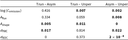

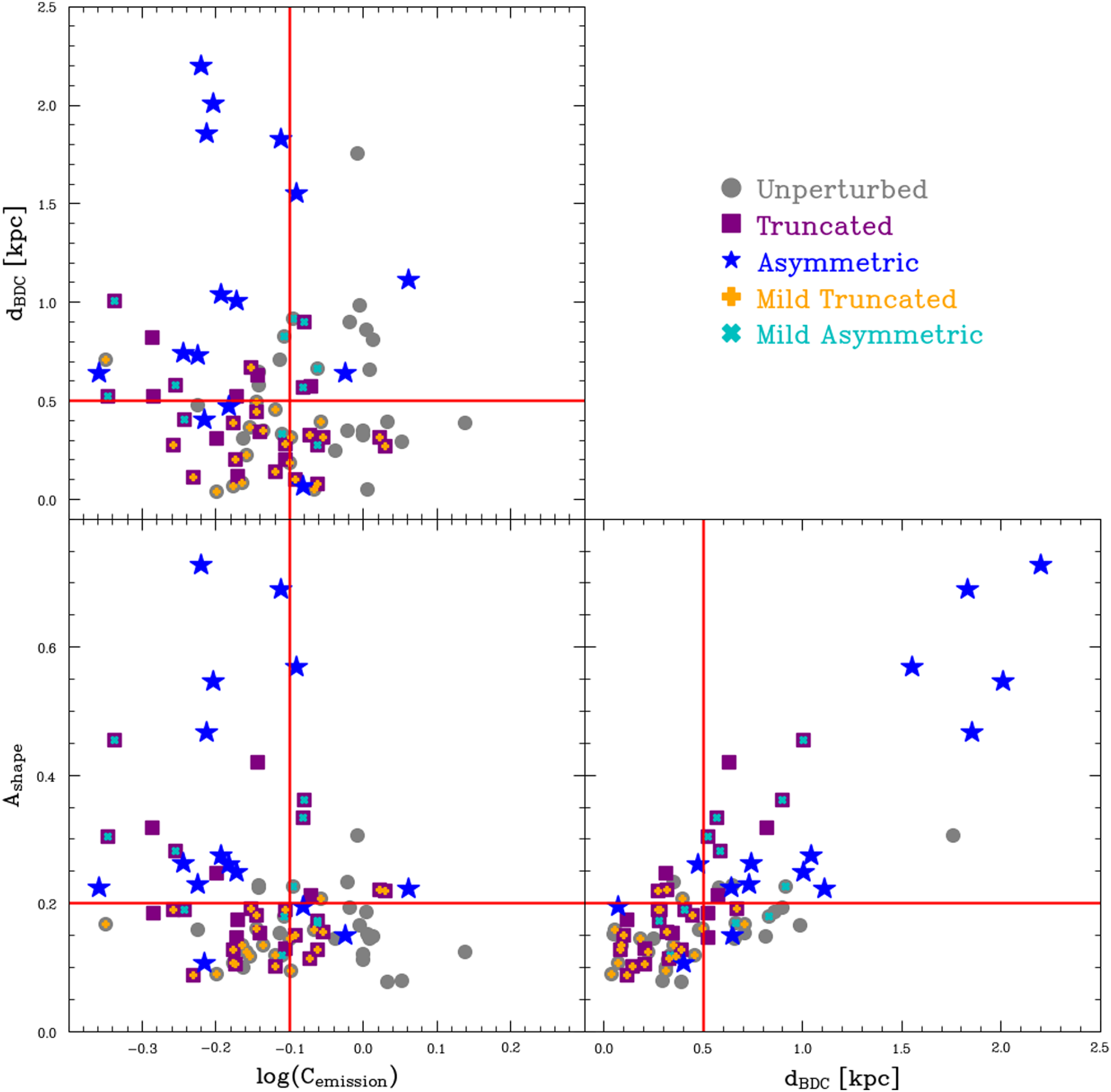


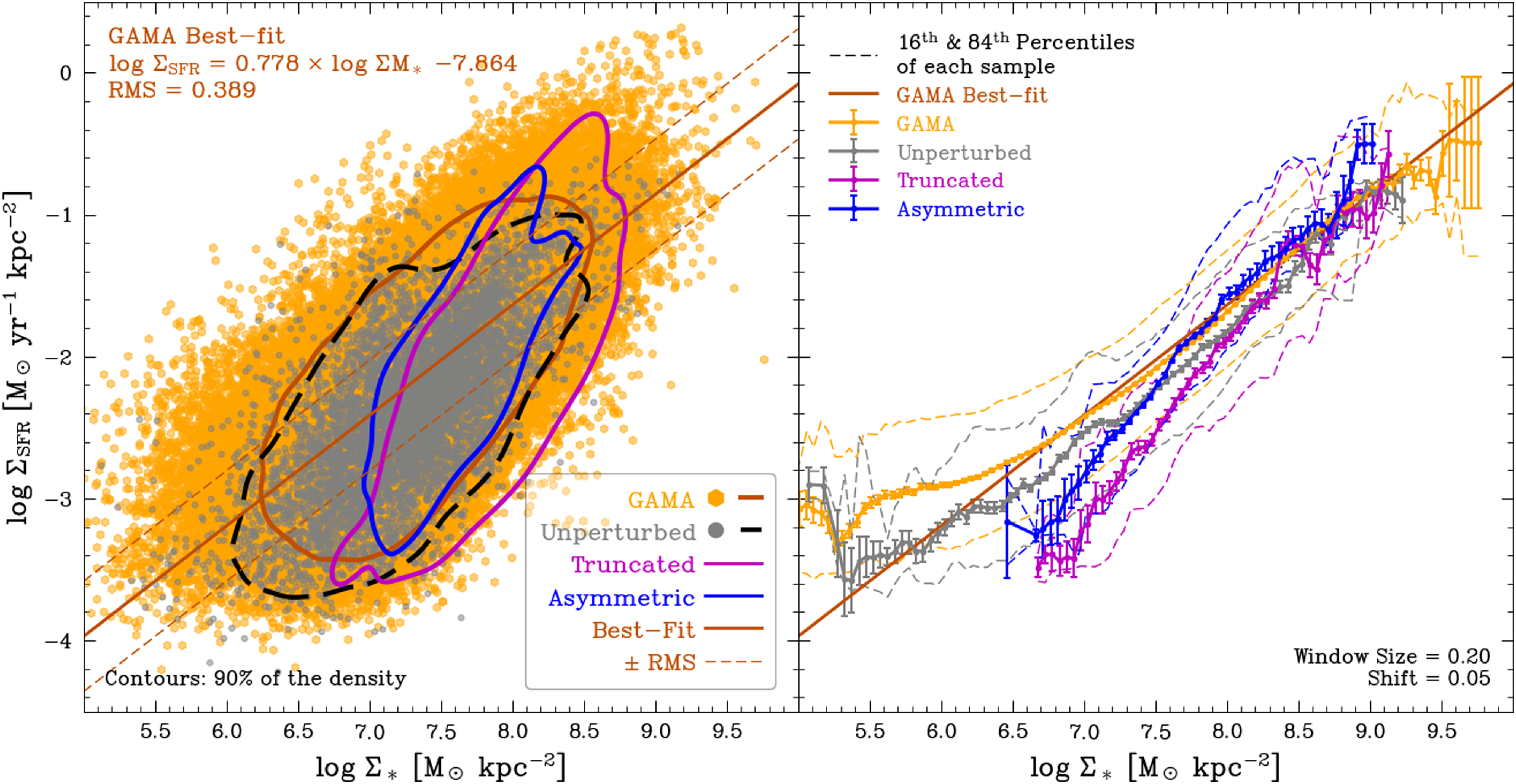


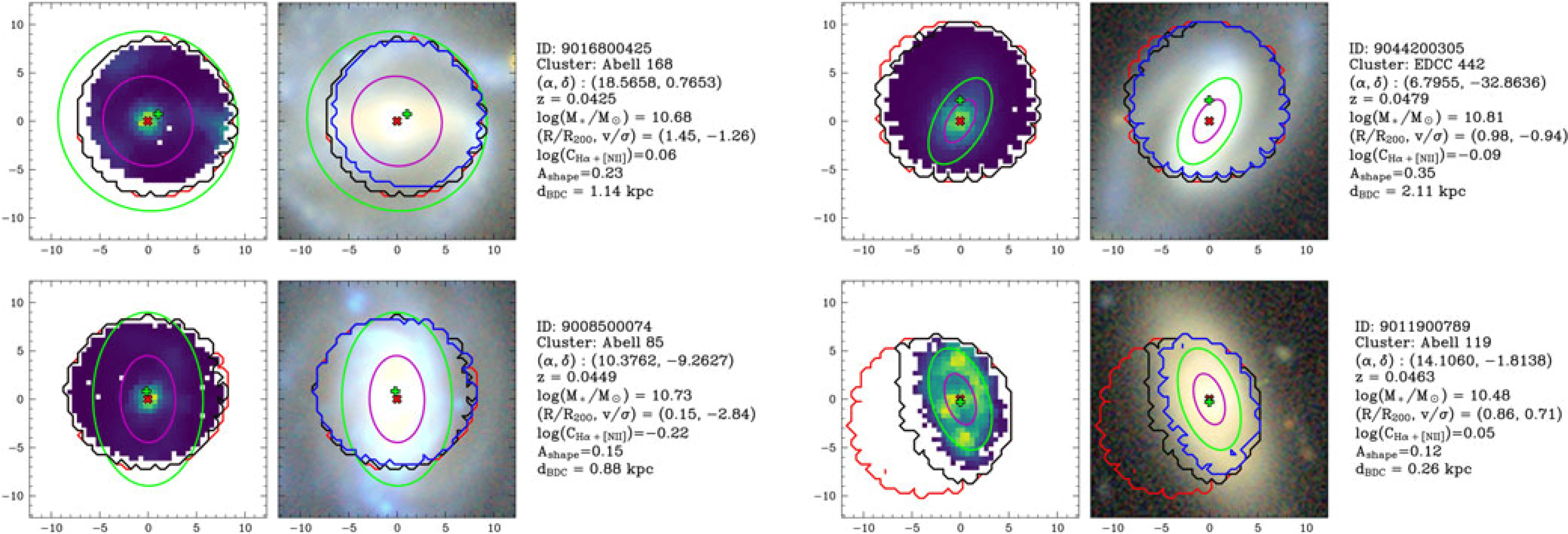

 Open access