


Impact statement
This study introduces a nonlinear system identification framework for wind turbines that bridges the gap between physics-based models and data-driven learning. By embedding interpretable surrogate aerodynamic models into control-oriented formulations, the method enables online adaptation to both freestream and waked conditions. The framework is experimentally validated and shown to enhance control performance compared to steady-state approaches and a BEM-based model in the present low Reynolds number setting. These findings advance the reliability of model-based wind turbine control and open perspectives for adaptive, data-centric strategies in wind farm operation, with potential to improve energy yield and resilience. In practice, this could support full-scale deployment through periodic model adaptation and integration into farm-level supervisory control systems.
1. Introduction
Wind energy is the fastest-growing renewable sector and a cornerstone of global decarbonization efforts. In Europe, the installed capacity has doubled from 128 GW in 2014 to 255 GW today (WindEurope, 2015, 2025). To meet rising demand, turbines have grown over tenfold in size and are increasingly clustered into large wind farms (Caduff et al., Reference Caduff, Huijbregts, Althaus, Koehler and Hellweg2012; Porté-Agel et al., Reference Porté-Agel, Bastankhah and Shamsoddin2020). As wind speed varies, wind turbines are controlled to maximize energy capture at low wind speeds, while constraining power output and mitigating structural loads at high wind speeds (Wright and Fingersh, Reference Wright and Fingersh2008).
Control of wind turbines has received enormous attention in recent years, with research increasingly focusing on advanced strategies. Approaches such as fuzzy logic control (FLC, Bharani and Sivaprakasam, Reference Bharani and Sivaprakasam2022; Borunda et al., Reference Borunda, Garduno, de la and Díaz2024; Maafa et al., Reference Maafa, Mellah, Benaouicha, Babes, Yahiou and Sahraoui2024), sliding mode control (SMC Echiheb et al., Reference Echiheb, Ihedrane, Bossoufi, Bouderbala, Motahhir, Masud, Aljahdali and ElGhamrasni2022; Zribi et al., Reference Zribi, Alrifai and Rayan2017), maximum power point tracking (MPPT Abdullah et al., Reference Abdullah, Yatim, Tan and Saidur2012; Pande and Nasikkar, Reference Pande and Nasikkar2023), and model predictive control (MPC Schlipf et al., Reference Schlipf, Schlipf and Kühn2013; Silva et al., Reference Silva, Ferrari and Wingerden2022)—have been proposed to enhance robustness and adaptability under varying conditions. However, their adoption remains limited due to practical challenges such as the need for expert tuning (FLC), high-frequency oscillations (SMC), sensitivity to wind fluctuations (MPPT), and computational demands (MPC). In recent years, AI-driven control approaches have emerged as a compelling alternative, leveraging data to design or adapt controllers capable of handling nonlinear, poorly modeled turbine dynamics (Tomin et al., Reference Tomin, Kurbatsky and Guliyev2019; Sierra-García and Santos, Reference Sierra-García and Santos2020). Methods based on artificial neural networks (ANN, Majout et al., Reference Majout, Bossoufi, Karim, Skruch, Mobayen, El Mourabit and Laggoun2024), adaptive neuro-fuzzy inference systems (ANFIS, Chhipa et al., Reference Chhipa, Kumar, Joshi, Chakrabarti, Jasinski, Burgio, Leonowicz, Jasinska, Soni and Chakrabarti2021), reinforcement learning (RL, Schena et al., Reference Schena, Gillyns, Munters, Buckingham and Mendez2022; Soler et al., Reference Soler, Mariño, Huergo, de and Ferrer2024), and evolutionary algorithms (GA, Guediri et al., Reference Guediri, Hettiri and Guediri2023, PSO Khurshid et al., Reference Khurshid, Mughal, Othman, Al-Hadhrami, Kumar, Khurshid, Arshad and Ahmad2022) have demonstrated promising performance in simulations. Nonetheless, their application in operational turbines remains constrained by stringent industry requirements for reliability, consistency, and certifiability (Chatterjee and Dethlefs, Reference Chatterjee and Dethlefs2021). Emerging directions such as safe reinforcement learning (Gu et al., Reference Gu, Yang, Du, Chen, Walter, Wang and Knoll2024) seek to address these barriers, although real-world deployment is still in its early stages.
Despite the growing interest in advanced controllers, classical model-based strategies remain the standard in industrial wind turbines due to their robustness and simplicity (Wright and Fingersh, Reference Wright and Fingersh2008; Pao and Johnson, Reference Pao and Johnson2009). Power maximization is traditionally carried out with torque controllers following the so-called
$ K{\omega}^2 $
 law, which adjusts the generator torque while maintaining a fixed, optimal blade pitch, whereas load mitigation is typically assigned to a proportional-integral (PI) controller of the blade pitch to sustain rated power output (Laks et al., Reference Laks, Pao and Wright2009). These typically rely on first-order nonlinear models, whose accuracy critically impacts performance. For example, the gain
$ K $
law, which adjusts the generator torque while maintaining a fixed, optimal blade pitch, whereas load mitigation is typically assigned to a proportional-integral (PI) controller of the blade pitch to sustain rated power output (Laks et al., Reference Laks, Pao and Wright2009). These typically rely on first-order nonlinear models, whose accuracy critically impacts performance. For example, the gain
$ K $
 in the
$ K{\omega}^2 $
in the
$ K{\omega}^2 $
 controller depends on the optimal tip-speed ratio (Pao and Johnson, Reference Pao and Johnson2009), while PI controllers are tuned using linearized turbine dynamics (Abbas et al., Reference Abbas, Zalkind, Pao and Wright2021). A persistent challenge is the identification of the rotor’s nonlinear aerodynamic behavior (Ribeiro et al., Reference Ribeiro, Casalino and Ferreira2023). Common approaches include generating aerodynamic maps via momentum theory—most notably the blade element momentum (BEM) method—or using pre-defined functional forms (e.g., polynomials or sinusoids) calibrated from experimental data (Pao and Johnson, Reference Pao and Johnson2009; Castillo et al., Reference Castillo, Andrade, Rivas and González2023). Accurate aerodynamic modeling is critical for minimizing energy losses in wind turbine control, with errors potentially reducing large-scale production by up to 3% (Pao and Johnson, Reference Pao and Johnson2009). Moreover, model accuracy degrades over time due to structural aging, blade erosion, and ice formation (Staffell and Green, Reference Staffell and Green2014; Campobasso et al., Reference Campobasso, Castorrini, Ortolani and Minisci2023). The continuous growth of turbine size and increasing wake interactions in large wind farms further challenge models originally designed for isolated turbines in steady inflow (Pao and Johnson, Reference Pao and Johnson2009; Shapiro et al., Reference Shapiro, Gayme and Meneveau2021): unsteady wake-induced conditions violate key assumptions of methods like BEM (Leishman, Reference Leishman2002), while blade flexibility alters aerodynamic load distributions beyond what standard models capture (Cao et al., Reference Cao, Shaler and Johnson2022). Though dynamic BEM introduces empirical corrections (Papi et al., Reference Papi, Jonkman, Robertson and Bianchini2023), persistent discrepancies with real-world behavior continue to motivate research into adaptive control and system identification (Pusch et al., Reference Pusch, Stockhouse, Abbas, Phadnis and Pao2024).
To address the limitations of first-principles models under real-world conditions, system identification techniques are increasingly employed in wind turbine control (Bossanyi et al., Reference Bossanyi, Savini, Iribas, Hau, Fischer, Schlipf, van Engelen, Rossetti and Carcangiu2012; Nelles, Reference Nelles2020). These data-driven approaches replace detailed physical modeling with parameter estimation from operational data (Rai et al., Reference Rai, Yang and Tsao2017). Most methods adopt linear state-space representations around specific operating points (Houtzager et al., Reference Houtzager, Kulscar, van Wingerden and Verhaegen2010). Examples include linear time-periodic (LTP) models identified via harmonic transfer functions using HAWC2 simulations (Allen et al., Reference Allen, Sracic, Chauhan and Hansen2011), and linear time-invariant (LTI) models estimated through predictor-based subspace identification (PBSID) (Houtzager et al., Reference Houtzager, Kulscar, van Wingerden and Verhaegen2010) or frequency domain decomposition of field data (Jasniewicz and Geyler, Reference Jasniewicz and Geyler2011). Simple auto-regressive (AR) models have also shown competitive accuracy with minimal parameters (Mahmoud and Qureshi, Reference Mahmoud and Qureshi2012). These linear models frequently support advanced control schemes such as model predictive control (MPC) (Verwaal et al., Reference Verwaal, Van Der Veen and Van Wingerden2015). Other strategies include adaptive second-order transfer functions (Simani and Castaldi, Reference Simani and Castaldi2013) and switching between LTI models across operating regions, with fuzzy logic used to smooth transitions (Jelavic et al., Reference Jelavic, Perc and Petrovic2006).
The limitations of linear control strategies under switching conditions are discussed in Gros and Schild, Reference Gros and Schild2017. Nonlinear models have demonstrated improved performance over traditional gain-scheduled PI controllers (Kumar and Stol, Reference Kumar and Stol2010), motivating system identification efforts using techniques such as variable-order fractional neural networks (Aslipour and Yazdizadeh, Reference Aslipour and Yazdizadeh2019), fuzzy systems (Simani, Reference Simani2012), and neural networks (Kelouwani and Agbossou, Reference Kelouwani and Agbossou2004). Clustering-based piecewise affine models have also been explored for power regulation (Sindareh Esfahani and Pieper, Reference Sindareh Esfahani and Pieper2021). However, concerns over generalization and reliability of these black-box methods have motivated hybrid methods that embed physical insights into data-driven models, improving robustness across operating conditions (Gebel et al., Reference Gebel, Rezaei, Vemuri, Liverud Krathe, Daems, Matthys, Sterckx, Vratsinis, Kestel, Nejad and Helsen2025).
A promising direction is the identification of physically interpretable quantities like power or thrust coefficients. Common approaches use polynomial models with recursive least squares (RLS) for real-time updates (Monroy and Alvarez-Icaza, Reference Monroy and Alvarez-Icaza2006; Hosseinpour et al., Reference Hosseinpour, Khosravi and Khaloozadeh2017), reduced multivariate polynomial models (Son et al., Reference Son, Lee and Park2009), or observer-based methods for dynamic estimation (Yap et al., Reference Yap, Dodson and Busawon2012). Adaptive systems such as adaptive neuro-fuzzy inference systems (ANFIS) have also been applied to optimize power coefficient estimation and enhance performance (Petković et al., Reference Petković, Ćojbašič and Nikolić2013; Asghar and Liu, Reference Asghar and Liu2017). Most adaptive modeling efforts for estimating the power coefficient have focused on isolated turbines and relied on numerical simulations where the true coefficient is known (Monroy and Alvarez-Icaza, Reference Monroy and Alvarez-Icaza2006; Petković et al., Reference Petković, Ćojbašič and Nikolić2013; Hosseinpour et al., Reference Hosseinpour, Khosravi and Khaloozadeh2017). To the authors’ knowledge, no studies have retrieved experimentally the power coefficient in the presence of turbine wakes, where conventional models typically fall back on simplified, low-fidelity wake descriptions (Bhatt et al., Reference Bhatt, Bernardoni, Leonardi and Zare2022). A notable exception is Annoni et al. (Reference Annoni, Howard, Seiler and Guala2015), who identified a two-turbine array offline using linear transfer functions from experimental data. However, online assimilation of the power coefficient in multi-turbine setups remains unaddressed.
This study addresses this gap by proposing an online experimental assimilation of the power coefficient for wind turbine arrays operating under wake interactions. The approach identifies a nonlinear, first-order dynamic model of the wind turbine array configuration, suitable for model-based control applications. As a demonstrative application, we consider a small-scale set-up of two 0.15 m diameter turbines, challenging the model to also recover low Reynolds number effects, and integrate the identified model into an adapted version of the
$ K{\omega}^2 $
 controller. Although demonstrated here on a small-scale experimental setup, the same identification logic is compatible with full-scale turbines, where operational SCADA data and inflow sensing could be used to update control-oriented surrogate models over time.
This article is organized as follows. First, the system identification problem of a wind turbine is reviewed in Section 2 while Section 3 introduces the proposed data-driven closure laws with the identification strategy. Section 4 describes the experimental setup. Section 5 presents the results while Section 6 closes with conclusions and perspectives.
2. System identification framework
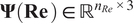
The configuration of interest is illustrated in Figure 1. It consists of identical turbines with radius
$ R $
 , aligned with the incoming flow and spaced at a distance
$ L $
, aligned with the incoming flow and spaced at a distance
$ L $
 , rotating at angular velocities
$ {\omega}_i $
, rotating at angular velocities
$ {\omega}_i $
 , subjected to an incoming flow
$ {u}_i $
, subjected to an incoming flow
$ {u}_i $
 , and experiencing aerodynamic torques
$ {\tau}_{\mathrm{aero},i} $
, and experiencing aerodynamic torques
$ {\tau}_{\mathrm{aero},i} $
 . The subscript
$ 1 $
. The subscript
$ 1 $
 denotes the first turbine exposed to the freestream wind. For a generic turbine
$ i $
denotes the first turbine exposed to the freestream wind. For a generic turbine
$ i $
 , the subscripts
$ i $
, the subscripts
$ i $
 and
$ i+1 $
and
$ i+1 $
 refer to two consecutive turbines in the array, with turbine
$ i+1 $
refer to two consecutive turbines in the array, with turbine
$ i+1 $
 operating in the wake of turbine
$ i $
operating in the wake of turbine
$ i $
 . We assume that the turbines operate under a power maximization objective in the torque-controlled region; therefore, the only relevant control inputs are the generator torques
$ {\tau}_{g,i} $
. We assume that the turbines operate under a power maximization objective in the torque-controlled region; therefore, the only relevant control inputs are the generator torques
$ {\tau}_{g,i} $
 .
.
Configuration of two aligned wind turbines and main variables. The downstream turbine, indexed by
$ i+1 $
 , operates in the wake of the upstream turbine
$ i $
, operates in the wake of the upstream turbine
$ i $
 , with inter-turbine spacing
$ L $
, with inter-turbine spacing
$ L $
 , rotor radius
$ R $
, rotor radius
$ R $
 , inflow velocity
$ {u}_i $
, inflow velocity
$ {u}_i $
 , aerodynamic torques
$ {\tau}_{\mathrm{aero},i} $
, aerodynamic torques
$ {\tau}_{\mathrm{aero},i} $
 and
$ {\tau}_{\mathrm{aero},i+1} $
and
$ {\tau}_{\mathrm{aero},i+1} $
 , and generator torques
$ {\tau}_{g,i} $
, and generator torques
$ {\tau}_{g,i} $
 and
$ {\tau}_{g,i+1} $
and
$ {\tau}_{g,i+1} $
 .
.

The aerodynamic torque generated by the turbines is related to the power coefficient
$ {C}_{p,i} $
 , defined as

where
$ {\tau}_{\mathrm{aero},i}\hskip0.1em {\omega}_i $
 represents the aerodynamic power extracted by turbine
$ i $
represents the aerodynamic power extracted by turbine
$ i $
 . In this work,
$ {C}_{p,i} $
. In this work,
$ {C}_{p,i} $
 is defined with respect to the freestream wind speed
$ {u}_1 $
is defined with respect to the freestream wind speed
$ {u}_1 $
 , so as to provide a consistent performance metric across the array. This differs from the local definition of the power coefficient, which would instead be based on the rotor-effective velocity experienced by each turbine, denoted here by
$ {u}_i $
, so as to provide a consistent performance metric across the array. This differs from the local definition of the power coefficient, which would instead be based on the rotor-effective velocity experienced by each turbine, denoted here by
$ {u}_i $
 .
.
The resulting nonlinear ODE model for a generic turbine
$ i $
 reads
reads

where the dot denotes time derivatives. The function
$ f $
 reads
reads

where
$ J $
 is the rotor moment of inertia [kg
$ \cdot $
is the rotor moment of inertia [kg
$ \cdot $
 m
$ {}^2 $
m
$ {}^2 $
 ] and
$ \rho $
] and
$ \rho $
 is the air density [kg
$ \cdot $
is the air density [kg
$ \cdot $
 m
$ {}^{-3} $
m
$ {}^{-3} $
 ]. The model considers the torque balance at the rotor level, without explicitly representing drivetrain dynamics.
The nonlinear system identification problem addressed in this work consists of modeling the power coefficients
$ {C}_{p,i} $
 in Equation (2.2) as general parametric functions
$ {\tilde{g}}_i\left(\cdot; {\mathbf{w}}_i\right) $
in Equation (2.2) as general parametric functions
$ {\tilde{g}}_i\left(\cdot; {\mathbf{w}}_i\right) $
 , where the parameters
$ {\mathbf{w}}_i\in {\mathrm{\mathbb{R}}}^{n_q} $
, where the parameters
$ {\mathbf{w}}_i\in {\mathrm{\mathbb{R}}}^{n_q} $
 act as closure variables. The power coefficient, therefore, plays the role of a closure term linking the aerodynamic power extraction to the rotor dynamics. The adopted closure laws distinguish between the upstream turbine and the downstream ones, and read

where
$ {\lambda}_i={\omega}_iR/{u}_1 $
 is the tip-speed ratio,
$ \Delta t=L/{u}_1 $
is the tip-speed ratio,
$ \Delta t=L/{u}_1 $
 denotes the estimated wake convection time,
$ \operatorname{Re}={u}_1D/\nu $
denotes the estimated wake convection time,
$ \operatorname{Re}={u}_1D/\nu $
 is the Reynolds number, and
$ \nu $
is the Reynolds number, and
$ \nu $
 is the air kinematic viscosity. In the present formulation, both the tip-speed ratio and the Reynolds number are defined using the freestream velocity
$ {u}_1 $
is the air kinematic viscosity. In the present formulation, both the tip-speed ratio and the Reynolds number are defined using the freestream velocity
$ {u}_1 $
 .
.
For a given geometry and fixed blade pitch angle, the power coefficient is commonly represented as a function of the tip-speed ratio
$ {\lambda}_i $
 , which motivates its inclusion in both upstream and downstream models. For the upstream turbine (
$ i=1 $
, which motivates its inclusion in both upstream and downstream models. For the upstream turbine (
$ i=1 $
 ), although full-scale machines are largely insensitive to Reynolds number variations at high Reynolds numbers (Saint-Drenan et al., Reference Saint-Drenan, Besseau, Jansen, Staffell, Troccoli, Dubus, Schmidt, Gruber, Simões and Heier2020), this dependence is retained here due to the small scale of the experimental setup (Bastankhah and Porté-Agel, Reference Bastankhah and Porté-Agel2017). For downstream turbines, wake effects are incorporated through a closure in which the influence of the upstream turbine is parameterized by its delayed tip-speed ratio
$ {\lambda}_{i-1}\left(t-\Delta t\right) $
), although full-scale machines are largely insensitive to Reynolds number variations at high Reynolds numbers (Saint-Drenan et al., Reference Saint-Drenan, Besseau, Jansen, Staffell, Troccoli, Dubus, Schmidt, Gruber, Simões and Heier2020), this dependence is retained here due to the small scale of the experimental setup (Bastankhah and Porté-Agel, Reference Bastankhah and Porté-Agel2017). For downstream turbines, wake effects are incorporated through a closure in which the influence of the upstream turbine is parameterized by its delayed tip-speed ratio
$ {\lambda}_{i-1}\left(t-\Delta t\right) $
 . This provides a compact, measurable, and control-relevant descriptor of the upstream operating condition, while avoiding the explicit introduction of local flow variables that are not directly accessible in the present experiments.
This formulation is a simplified model of wake interactions, as it does not resolve spatial wake structure, partial overlap, yaw misalignment, or atmospheric shear. It is therefore mainly intended for aligned configurations and controlled inflow, where the downstream turbine response is dominated by the upstream operating state. Nevertheless, the general adjoint-based online adaptation framework is more general and can be extended with additional variables when more detailed flow information and more general dynamic wake models are available.
Denoting by
$ \mathbf{w}=\left[{\mathbf{w}}_1,{\mathbf{w}}_2,\dots \right]\in {\mathrm{\mathbb{R}}}^{n_q} $
 the concatenated parameter vector of all turbines, the identification is performed by minimizing the discrepancy between observed data and model predictions. Following a variational approach (PA; Schena et al., Reference Schena, Marques, Poletti, Ahizi, JVd and Mendez2023; Marques et al., Reference Marques, Ahizi and Mendez2024), the optimal parameters minimize the cost functional

where
$ {L}_p $
 quantifies the mismatch between the simulated state
$ {\omega}_i\left(t;{\mathbf{w}}_i\right) $
quantifies the mismatch between the simulated state
$ {\omega}_i\left(t;{\mathbf{w}}_i\right) $
 and the measured rotor speed
$ {\omega}_i^{\ast }(t) $
and the measured rotor speed
$ {\omega}_i^{\ast }(t) $
 . The time interval
$ {T}_0 $
. The time interval
$ {T}_0 $
 represents the observation window (episode). In the proposed framework, data are acquired in real time during each episode, whereas parameter updates are performed only at the end of the episode by solving the batch optimization problem in Equation (2.5). The method should therefore be interpreted as an episodic online adaptation strategy. As detailed in the following section, the identification is carried out independently for each turbine.
3. Power coefficient closure laws
For the first turbine
$ \left(i=1\right) $
 , the power coefficient is modeled as

whereas for the downstream turbines
$ \left(i>1\right) $
 , it is modeled as

where, consistently with Section 2, the upstream tip-speed ratio is evaluated at a delayed time, i.e.,
$ {\lambda}_{i-1}={\lambda}_{i-1}\left(t-\Delta t\right) $
 . The coefficients
$ {w}_{i,m,n} $
. The coefficients
$ {w}_{i,m,n} $
 are collected in the vector
$ {\mathbf{w}}_i $
are collected in the vector
$ {\mathbf{w}}_i $
 for each turbine. The functions
$ {\phi}_m $
for each turbine. The functions
$ {\phi}_m $
 and
$ {\psi}_n $
and
$ {\psi}_n $
 denote radial basis functions (RBFs) and polynomial basis functions, respectively, as described in detail below. The integers
$ M $
denote radial basis functions (RBFs) and polynomial basis functions, respectively, as described in detail below. The integers
$ M $
 and
$ N $
and
$ N $
 represent the total number of basis functions used. As demonstrated in the following, the proposed formulation allows for representing a realistic nonlinear power coefficient curve while maintaining a linear dependency on the model parameters.
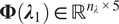
The functions
$ {\phi}_m\left(\lambda; {\lambda}_m^{\ast },{c}_m\right) $
 and
$ {\psi}_n(x) $
and
$ {\psi}_n(x) $
 act as basis functions. The first is a basis of compact support radial basis functions (RBFs)

where
$ {d}_m\left(\lambda \right)=\lambda -{\lambda}_m^{\ast } $
 is the distance from the RBF center
$ {\lambda}_m^{\ast } $
is the distance from the RBF center
$ {\lambda}_m^{\ast } $
 , and
$ {c}_m $
, and
$ {c}_m $
 is the basis radius. Five of these bases are collocated in the range of admissible tip-speed ratios at centers
$ {\lambda}_m^{\ast }=\left[\mathrm{4,5,6,7,8}\right] $
is the basis radius. Five of these bases are collocated in the range of admissible tip-speed ratios at centers
$ {\lambda}_m^{\ast }=\left[\mathrm{4,5,6,7,8}\right] $
 , all having the same shape factor
$ {c}_m=1.5 $
, all having the same shape factor
$ {c}_m=1.5 $
 . The number of RBFs was chosen as a compromise between ensuring sufficient flexibility to represent the useful portion of the power coefficient curve and avoiding an unnecessarily large number of basis functions. A polynomial basis up to order
$ 2 $
. The number of RBFs was chosen as a compromise between ensuring sufficient flexibility to represent the useful portion of the power coefficient curve and avoiding an unnecessarily large number of basis functions. A polynomial basis up to order
$ 2 $
 is chosen, hence
$ {\psi}_n(x)={x}^n $
is chosen, hence
$ {\psi}_n(x)={x}^n $
 with
$ n=\left[\mathrm{0,1,2}\right] $
with
$ n=\left[\mathrm{0,1,2}\right] $
 . This choice was found sufficient to capture the observed dependence on the second variable while preserving a parsimonious parametrization. A more systematic sensitivity study on the number of basis functions could be considered in future works.
3.1. Initial guess for model parameters
An estimate of the coefficients
$ {w}_{i,m,n} $
 can be computed using a standard least squares approach under the assumption of steady-state operation, i.e.,
$ {\dot{\omega}}_i=0 $
can be computed using a standard least squares approach under the assumption of steady-state operation, i.e.,
$ {\dot{\omega}}_i=0 $
 . Under this condition, Equation (2.3) yields
$ {\tau}_{a,i}={\tau}_{g,i} $
. Under this condition, Equation (2.3) yields
$ {\tau}_{a,i}={\tau}_{g,i} $
 . Substituting this relation into Equation (2.1), one obtains

Assuming that
$ {\tau}_{g,i} $
 ,
$ {\omega}_i $
,
$ {\omega}_i $
 and
$ {u}_1 $
and
$ {u}_1 $
 are measured, Equation (3.4) can be used to compute
$ {C}_{p,i} $
are measured, Equation (3.4) can be used to compute
$ {C}_{p,i} $
 , allowing for deriving initial guesses to train the surrogate models in Equations (3.1) and (3.2) via least squares regression. For instance, in the case of the first turbine in Equation (3.1), collecting a grid of
$ {n}_{\lambda}\times {n}_{Re} $
, allowing for deriving initial guesses to train the surrogate models in Equations (3.1) and (3.2) via least squares regression. For instance, in the case of the first turbine in Equation (3.1), collecting a grid of
$ {n}_{\lambda}\times {n}_{Re} $
 training samples, with
$ {n}_{\lambda } $
training samples, with
$ {n}_{\lambda } $
 and
$ {n}_{Re} $
and
$ {n}_{Re} $
 the number of tip speed ratios and Reynolds numbers in the grid, and enforcing Equation (3.4) in each of the grid points yields a matrix factorization of the form

where
$ {\boldsymbol{C}}_{p,1}\in {\mathrm{\mathbb{R}}}^{n_{\lambda}\times {n}_{Re}} $
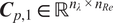 is the matrix of power coefficients computed from Equation (3.4) at all training points. The matrix
$ \boldsymbol{\Phi} \left({\boldsymbol{\lambda}}_1\right)\in {\mathrm{\mathbb{R}}}^{n_{\lambda}\times 5} $
is the matrix of power coefficients computed from Equation (3.4) at all training points. The matrix
$ \boldsymbol{\Phi} \left({\boldsymbol{\lambda}}_1\right)\in {\mathrm{\mathbb{R}}}^{n_{\lambda}\times 5} $
 is the radial basis function (RBF) matrix evaluated at the tip-speed ratios
$ {\boldsymbol{\lambda}}_1 $
is the radial basis function (RBF) matrix evaluated at the tip-speed ratios
$ {\boldsymbol{\lambda}}_1 $
 , while
$ \boldsymbol{\Psi} \left(\mathbf{\operatorname{Re}}\right)\in {\mathrm{\mathbb{R}}}^{n_{Re}\times 3} $
, while
$ \boldsymbol{\Psi} \left(\mathbf{\operatorname{Re}}\right)\in {\mathrm{\mathbb{R}}}^{n_{Re}\times 3} $
 contains the polynomial basis evaluated at the Reynolds numbers
$ \mathbf{\operatorname{Re}}\in {\mathrm{\mathbb{R}}}^{n_{Re}} $
contains the polynomial basis evaluated at the Reynolds numbers
$ \mathbf{\operatorname{Re}}\in {\mathrm{\mathbb{R}}}^{n_{Re}} $
 . The coefficient matrix
$ {\boldsymbol{w}}_1\in {\mathrm{\mathbb{R}}}^{5\times 3} $
. The coefficient matrix
$ {\boldsymbol{w}}_1\in {\mathrm{\mathbb{R}}}^{5\times 3} $
 , with entries
$ {w}_{1,m,n} $
, with entries
$ {w}_{1,m,n} $
 , contains the parameters to be identified in the surrogate model Equation (3.1) and de facto encodes the performances of the turbine under the dynamical system in Equations (2.2)–(2.3).
These coefficients can be computed by pseudo-inverse on both sides of Equation (3.5):

where
$ {\boldsymbol{w}}_{1,0} $
 emphasizes that these are the initial guesses for the optimization.
Considering that this estimate acts only as an initial guess, no regularization was used in the least square solution. On the other hand, taking into account the measurement uncertainties was found to improve the initial guess. These were introduced using a classic weighted formulation on the regression of the RBF block, which reads

where the matrix
$ \mathbf{N} $
 is an estimate of the measurement precision, giving more weight to points with lower uncertainty and defined as

where
$ {\sigma}_j^2 $
 is the variance of each measurement and
$ {\sigma}_{\mathrm{min}}=\min \left\{{\sigma}_i\right\} $
is the variance of each measurement and
$ {\sigma}_{\mathrm{min}}=\min \left\{{\sigma}_i\right\} $
 . These were used by propagating the measurement uncertainties of
$ {u}_i $
. These were used by propagating the measurement uncertainties of
$ {u}_i $
 ,
$ {\tau}_{g,i} $
,
$ {\tau}_{g,i} $
 and
$ {\omega}_i $
and
$ {\omega}_i $
 through Equation (3.4) using a standard first-order approach. A comparison between weighted and unweighted regressions shows that the inclusion of measurement uncertainties leads to an improvement of approximately 10% in the uncertainty-weighted error (wRMSE), indicating a better agreement with the most reliable data. The solution of the initial set of coefficients from Equation (3.7) can be interpreted as first carry out a weighted least square regression of the model
$ {\mathbf{C}}_{\mathbf{p},\mathbf{1}}=\boldsymbol{\Phi} \mathbf{A} $
through Equation (3.4) using a standard first-order approach. A comparison between weighted and unweighted regressions shows that the inclusion of measurement uncertainties leads to an improvement of approximately 10% in the uncertainty-weighted error (wRMSE), indicating a better agreement with the most reliable data. The solution of the initial set of coefficients from Equation (3.7) can be interpreted as first carry out a weighted least square regression of the model
$ {\mathbf{C}}_{\mathbf{p},\mathbf{1}}=\boldsymbol{\Phi} \mathbf{A} $
 , followed by a traditional least square regression of the model
$ {\mathbf{A}}^T=\boldsymbol{\Psi} {\boldsymbol{w}}_{1,0}^T $
, followed by a traditional least square regression of the model
$ {\mathbf{A}}^T=\boldsymbol{\Psi} {\boldsymbol{w}}_{1,0}^T $
 .
.
3.2. Model parameters obtained from a BEM-based model
In order to provide a reference model for comparison, the same parametrization described in Section 3.1 was also constructed using data generated from a classical Blade Element Momentum (BEM) approach. The motivation for introducing a BEM-based model is that it represents the standard tool used in the wind energy community to derive aerodynamic models for control-oriented applications.
In this case, instead of relying on experimental measurements, a grid of operating conditions was generated numerically. In particular, the power coefficient
$ {C}_{p,1} $
 was evaluated over a set of tip-speed ratios
$ {\lambda}_1 $
was evaluated over a set of tip-speed ratios
$ {\lambda}_1 $
 and Reynolds numbers
$ \operatorname{Re} $
and Reynolds numbers
$ \operatorname{Re} $
 , forming a synthetic dataset analogous to
$ {\boldsymbol{C}}_{p,1} $
, forming a synthetic dataset analogous to
$ {\boldsymbol{C}}_{p,1} $
 in Equation (3.5). The aerodynamic polars of the airfoil, i.e., lift and drag coefficients as a function of the angle of attack, were computed using XFOIL at different Reynolds numbers. These polars were then used within a BEM framework to evaluate the turbine performance, using the CcBlade module from the WISDEM Python package (Ning, Reference Ning2013).
Given this dataset, the same regression framework as in Section 3.1 was employed. In particular, the coefficient matrix was obtained by solving a least squares problem of the form

where
$ {\boldsymbol{C}}_{p,1}^{\mathrm{BEM}} $
 denotes the matrix of power coefficients obtained from the BEM simulations. The corresponding model coefficients
$ {\boldsymbol{w}}_1^{\mathrm{BEM}} $
denotes the matrix of power coefficients obtained from the BEM simulations. The corresponding model coefficients
$ {\boldsymbol{w}}_1^{\mathrm{BEM}} $
 are computed analogously to Equation (3.6). In this case, no weighting based on measurement uncertainty is introduced, as the dataset is generated numerically.
It is important to note that, although BEM models are widely used and well established for utility-scale wind turbines, their application in the present context must be treated with care. The experiments considered in this work are conducted at a small scale, corresponding to relatively low Reynolds numbers. Under these conditions, the aerodynamic behavior is more difficult to predict accurately, which may result in larger discrepancies. Therefore, the predictions obtained from the BEM-based model in the present study should be interpreted with caution, as they may be significantly less reliable than those usually obtained for conventional full-scale wind turbines.
Finally, it is worth noting that extending the BEM framework to the downstream turbine is not straightforward, due to the presence of wake interactions and the need for an additional wake model. Since this is not the focus of the present study, the BEM-based parametrization is considered here only for the first turbine and is used solely as a reference for comparison purposes.
3.3. A note on local stability
The local stability properties of the steady-state solutions defined by
$ {\tau}_{a,i}={\tau}_{g,i} $
 in Equation (2.3) can be assessed by linearizing the rotor dynamics around a given equilibrium point. Since the control input acts on the tip-speed ratio through the rotor speed, the relevant condition is expressed in terms of the local slope of the net torque with respect to
$ {\lambda}_i $
in Equation (2.3) can be assessed by linearizing the rotor dynamics around a given equilibrium point. Since the control input acts on the tip-speed ratio through the rotor speed, the relevant condition is expressed in terms of the local slope of the net torque with respect to
$ {\lambda}_i $
 . In open-loop operation, the system generally admits a family of equilibrium points, parameterized by the operating conditions. For a generic turbine
$ i $
. In open-loop operation, the system generally admits a family of equilibrium points, parameterized by the operating conditions. For a generic turbine
$ i $
 , local asymptotic stability of a given equilibrium requires

where the derivative is evaluated with the operating conditions held fixed, namely the freestream velocity
$ {u}_1 $
 and, for downstream turbines, the upstream tip-speed ratio
$ {\lambda}_{i-1} $
and, for downstream turbines, the upstream tip-speed ratio
$ {\lambda}_{i-1} $
 .
.
It is important to note that, in open-loop operation, not all equilibrium points are necessarily stable. Depending on the operating region, unstable equilibria may also arise. For this reason, stability was not explicitly enforced as a global constraint during identification. Instead, the optimization relies on matching the measured rotor trajectories in the operating regions explored by the data. As a consequence, parameter choices associated with incorrect local stability properties tend to produce trajectories that are inconsistent with the experimental observations, and are therefore penalized by the cost functional. As shown later in the results, this mechanism plays a visible role in the optimization process, where even limited parameter updates may lead to marked changes in the model response once dynamically consistent local behavior is recovered.
3.4. Adjoint-based identification
In this work, the Lagrangian in Equation (2.5) is defined as

The optimization for each turbine is performed independently. This is possible because, in the identification of a downstream turbine, the upstream tip-speed ratio
$ {\lambda}_{i-1} $
 is treated as a measured exogenous input. Therefore, the model of turbine
$ i $
is treated as a measured exogenous input. Therefore, the model of turbine
$ i $
 can be identified separately once the corresponding upstream trajectory is provided from the experimental data. The measured time series
$ {\omega}_i^{\ast }(t) $
can be identified separately once the corresponding upstream trajectory is provided from the experimental data. The measured time series
$ {\omega}_i^{\ast }(t) $
 is filtered using a
$ {4}^{\mathrm{th}} $
is filtered using a
$ {4}^{\mathrm{th}} $
 order a Butterworth low-pass filter with a cutoff frequency of
$ {f}_{\mathrm{c}.\mathrm{o}.}=2\hskip0.22em \mathrm{Hz} $
order a Butterworth low-pass filter with a cutoff frequency of
$ {f}_{\mathrm{c}.\mathrm{o}.}=2\hskip0.22em \mathrm{Hz} $
 chosen based on the turbine’s time response to attenuate high-frequency noise.
The cost functions
$ {\mathcal{J}}_{w,i}\left({\mathbf{w}}_i\right) $
 are optimized using the Adam optimizer (Kingma and Ba, Reference Kingma and Ba2014), preferred over quasi-Newton alternatives such as the BFGS because of its higher robustness to gradient noise. The gradient
$ {\nabla}_{\mathbf{w},i}{\mathcal{J}}_{w,i} $
are optimized using the Adam optimizer (Kingma and Ba, Reference Kingma and Ba2014), preferred over quasi-Newton alternatives such as the BFGS because of its higher robustness to gradient noise. The gradient
$ {\nabla}_{\mathbf{w},i}{\mathcal{J}}_{w,i} $
 was computed via an adjoint-based formulation (Sengupta et al., Reference Sengupta, Friston and Penny2014) to avoid solving
$ {n}_w $
was computed via an adjoint-based formulation (Sengupta et al., Reference Sengupta, Friston and Penny2014) to avoid solving
$ {n}_w $
 additional ODEs per evaluation. The adjoint method computes the gradient as

where
$ {s}_{\lambda }(t) $
 are the adjoint variables. These are obtained by solving the adjoint terminal value problem

where all terms are evaluated at the current guess for the states
$ {\omega}_i\left(t;{\mathbf{w}}_i\right) $
 , which thus requires first a forward integration. We note that the transposition in Equation (3.13) is included for consistency with high dimensional problems but is irrelevant to the problem at hand since both Jacobians are scalars. The adjoint-based evaluation requires one forward pass and one backward pass, regardless of the number of unknown parameters
$ {\mathbf{w}}_i $
, which thus requires first a forward integration. We note that the transposition in Equation (3.13) is included for consistency with high dimensional problems but is irrelevant to the problem at hand since both Jacobians are scalars. The adjoint-based evaluation requires one forward pass and one backward pass, regardless of the number of unknown parameters
$ {\mathbf{w}}_i $
 .
.
Starting from the initialization as in Equation (3.7), the gradient computation is used then to update the weight guess using the ADAM optimizer (Kingma and Ba, Reference Kingma and Ba2014)

where
$ n $
 is the iteration number,
$ \eta $
is the iteration number,
$ \eta $
 is the learning rate,
$ \unicode{x025B} $
is the learning rate,
$ \unicode{x025B} $
 is a small constant to prevent division by zero, and
$ \hat{\mathbf{m}} $
is a small constant to prevent division by zero, and
$ \hat{\mathbf{m}} $
 and
$ \hat{\mathbf{v}} $
and
$ \hat{\mathbf{v}} $
 are filtered momentum parameters computed as follows:


where
$ \mathbf{m} $
 and
$ \mathbf{v} $
and
$ \mathbf{v} $
 are the first and second moment estimates of the gradient, while
$ {\beta}_1 $
are the first and second moment estimates of the gradient, while
$ {\beta}_1 $
 and
$ {\beta}_2 $
and
$ {\beta}_2 $
 are the decay rate coefficients for the moments.
Multiple restarts were employed to reset the optimization process whenever a sudden jump in the cost function occurred, typically because the current parameter guess violates the stability condition in Equation (3.10). In such a case, the optimization is restarted to reset the low-pass filtering of the gradient. Additionally, a learning rate schedule was designed to reduce the learning rate once the cost function falls below a predefined threshold. This approach allows the optimizer to take smaller steps and prevent overshooting. It is worth noting that, while uncertainty weighting is introduced in the construction of the initial guess (Section 3.1), it is not explicitly propagated in the adjoint-based dynamic identification. This choice is motivated by the fact that the initial reconstruction of the power coefficient is highly sensitive to measurement noise, particularly due to the cubic dependence on wind speed. In contrast, the dynamic identification relies on the rotor speed signal, which is measured with lower uncertainty, and whose dynamics inherently filter high-frequency fluctuations.
4. Experimental methodology
The detailed experimental setup used to acquire data and interact with the system in real time is described in Section 4.1. The identification methodology is evaluated across multiple scenarios. The first, detailed in Section 4.2, focuses on nonlinear system identification for two turbines operating under low turbulence conditions with varying set points. The second scenario, presented in Section 4.3, simulates a wind farm environment with high turbulence intensity and fixed operating conditions. Finally, the robustness of the identified models is assessed through a control task, as described in Section 4.4.
4.1. Experimental set up
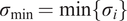
The proposed methodology was experimentally validated using three-bladed wind turbine scale models, originally designed in Coudou et al. (Reference Coudou, Buckingham, Bricteux and Beeck2018). Each model features a rotor diameter of
$ D=0.15\hskip0.22em \mathrm{m} $
 and a hub height of
$ {z}_{\mathrm{hub}}=0.13\hskip0.22em \mathrm{m} $
and a hub height of
$ {z}_{\mathrm{hub}}=0.13\hskip0.22em \mathrm{m} $
 . The rotor was designed based on Burton’s optimal rotor theory (Sørensen and Sørensen, Reference Sørensen and Sørensen2016) and employs a low-Reynolds-number airfoil section (HAM-STD HS1–606). This design enables the turbines to achieve power and thrust coefficient performances comparable to those of full-scale turbines such as the Vestas V66-2 MW offshore turbine, of which it represents a 1:440 scale version. A photograph of the turbines is shown in Figure 2 together with the relevant dimensions and airfoil section. The total moment of inertia of the rotor has been estimated from the CAD model to be
$ J=2.5\times {10}^{-6} $
. The rotor was designed based on Burton’s optimal rotor theory (Sørensen and Sørensen, Reference Sørensen and Sørensen2016) and employs a low-Reynolds-number airfoil section (HAM-STD HS1–606). This design enables the turbines to achieve power and thrust coefficient performances comparable to those of full-scale turbines such as the Vestas V66-2 MW offshore turbine, of which it represents a 1:440 scale version. A photograph of the turbines is shown in Figure 2 together with the relevant dimensions and airfoil section. The total moment of inertia of the rotor has been estimated from the CAD model to be
$ J=2.5\times {10}^{-6} $
 kg m
$ {}^2 $
kg m
$ {}^2 $
 .
.
Wind turbine model used in the experimental campaign (Coudou et al., Reference Coudou, Buckingham, Bricteux and Beeck2018) and corresponding low-Reynolds-number airfoil used in the blade.
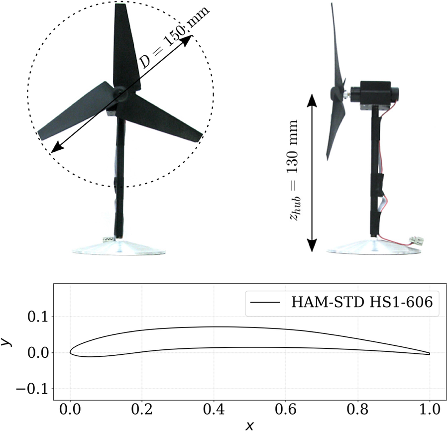
Figure 2. Long description
At the top left, a front view photo shows a three-blade wind turbine mounted on a vertical stand with a circular base. A dashed circle marks the rotor diameter labeled D equals 150 millimeters. At the top right, a side view photo displays the same turbine, highlighting the hub height labeled z sub hub equals 130 millimeters. Below, a line graph plots the airfoil profile used for the blade, labeled HAM-STD H S 1-606. The x axis ranges from 0 to 1, and the y axis from minus 0.1 to 0.1. The airfoil curve is cambered, with maximum thickness near x equals 0.3.
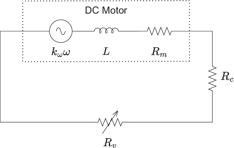
Each rotor is directly coupled to a DC motor (Faulhaber 1331T006SR) operating as a generator. The blades are fixed, hence the only actuation is through motor torque, adjusted via a variable resistance
$ {R}_{\mathrm{v}} $
 connected to the generator. The generator torque
$ {\tau}_g $
connected to the generator. The generator torque
$ {\tau}_g $
 is modeled electrically by relating it to the current
$ i $
is modeled electrically by relating it to the current
$ i $
 as
$ {\tau}_g={k}_{\tau}\cdot i $
as
$ {\tau}_g={k}_{\tau}\cdot i $
 where
$ {k}_{\tau } $
where
$ {k}_{\tau } $
 is a motor constant. The back electromotive force (EMF) is assumed proportional to the rotor speed:
$ {V}_{\mathrm{emf}}={k}_{\omega}\cdot \omega, $
is a motor constant. The back electromotive force (EMF) is assumed proportional to the rotor speed:
$ {V}_{\mathrm{emf}}={k}_{\omega}\cdot \omega, $
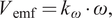 with
$ {k}_{\omega } $
with
$ {k}_{\omega } $
 also a motor-specific constant. Neglecting generator inductance
$ L $
also a motor-specific constant. Neglecting generator inductance
$ L $
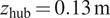
 and applying mesh analysis to the equivalent circuit (Figure 3), the generator torque becomes:

where
$ {R}_{\mathrm{tot}}={R}_{\mathrm{m}}+{R}_{\mathrm{c}} $
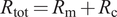 , with
$ {R}_{\mathrm{m}} $
, with
$ {R}_{\mathrm{m}} $
 and
$ {R}_{\mathrm{c}} $
and
$ {R}_{\mathrm{c}} $
 representing the internal motor and cable resistances, respectively. This relation is used in Equation (2.3) to compute the mechanical torque on the turbine shaft.
Electrical model of the wind turbine generator and relevant variables.
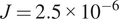
The experimental setup with sensors and controllers is illustrated in Figure 4 for the case of two turbines. A Raspberry Pi 4 is employed for real-time data acquisition and turbines’ control. Each turbine is equipped with an incremental encoder for measuring the rotational speed
$ {\omega}_i^{\ast }(t) $
 . These encoders feature 50 pulses per revolution (PPR), and the rotational speed is computed by an Arduino Nano through the measurement of the time interval between two consecutive pulses.
Experimental setup in the low-turbulence scenario configuration, detailing the measurement of free-stream wind speed
$ {u}_1 $
 , rotational speed
$ {\omega}_i^{\ast } $
, rotational speed
$ {\omega}_i^{\ast } $
 of each turbine, and torque actuation via variable resistance
$ {R}_{v,i} $
of each turbine, and torque actuation via variable resistance
$ {R}_{v,i} $
 controlled by a 12-bit binary signal
$ {a}_{bin,i} $
controlled by a 12-bit binary signal
$ {a}_{bin,i} $
 .
.
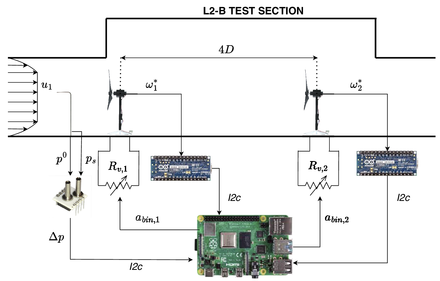
Figure 4. Long description
At the far left, arrows indicate free-stream wind speed labeled u sub 1 entering the L2-B test section. Immediately downstream, a pressure sensor measures p super 0 and p sub s, with the differential pressure labeled delta p. The airflow passes two wind turbines spaced 4 D apart, each labeled with rotational speed omega sub 1 super star and omega sub 2 super star. Below each turbine, variable resistors R sub v comma 1 and R sub v comma 2 are shown, each controlled by a microcontroller board. Binary signals a sub bin comma 1 and a sub bin comma 2 regulate the resistors. All microcontrollers and the pressure sensor are connected via I 2 C communication lines to a central processing unit, depicted as a Raspberry Pi. The schematic details the measurement and control flow for wind speed, turbine rotation, and torque actuation.
The free-stream wind speed at hub height
$ {u}_1\left({z}_{\mathrm{hub}},t\right) $
 is measured using a Prandtl tube. The dynamic pressure
$ \Delta p=\frac{1}{2}\rho {u}_1^2 $
is measured using a Prandtl tube. The dynamic pressure
$ \Delta p=\frac{1}{2}\rho {u}_1^2 $
 , defined as the difference between total
$ {p}^0 $
, defined as the difference between total
$ {p}^0 $
 and static pressure
$ {p}_s $
and static pressure
$ {p}_s $
 , is acquired using an AMS 5812–0000-DB sensor, from which the wind speed is then derived
$ {u}_1=\sqrt{2\Delta p/\rho } $
, is acquired using an AMS 5812–0000-DB sensor, from which the wind speed is then derived
$ {u}_1=\sqrt{2\Delta p/\rho } $
 . A thermocouple is installed to monitor air temperature and enhance the accuracy of air density estimations.
Torque actuation is implemented by modulating the electrical load through a bank of 12 resistors, each controlled via MOSFETs. This configuration enables
$ {2}^{12} $
 discrete resistance values, ranging from 0.25
$ \Omega $
discrete resistance values, ranging from 0.25
$ \Omega $
 to 1024
$ \Omega $
to 1024
$ \Omega $
 . A 12-bit binary signal
$ {a}_{bin} $
. A 12-bit binary signal
$ {a}_{bin} $
 is sent from the Raspberry Pi 4 to a shift register (SNx4HC595), which selects the active resistors. The corresponding resistance
$ {R}_{\mathrm{v}} $
is sent from the Raspberry Pi 4 to a shift register (SNx4HC595), which selects the active resistors. The corresponding resistance
$ {R}_{\mathrm{v}} $
 is retrieved from a precomputed lookup table.
4.2. Low turbulence scenario identification
The first scenario evaluates the proposed methodology for identifying the aerodynamical characteristics of two wind turbine models in a tandem configuration, where the operational conditions of both turbines are varied (Figure 4). This identification under varying conditions is used for the control implementation, as discussed in Section 4.4. The two wind turbine models are separated by four rotor diameters (
$ 4D\approx 60 $
 cm). The experimental campaign was conducted in the VKI Wind Engineering facility L2-B, an open-circuit wind tunnel with a test section of dimensions
$ H=0.5\mathrm{m} $
cm). The experimental campaign was conducted in the VKI Wind Engineering facility L2-B, an open-circuit wind tunnel with a test section of dimensions
$ H=0.5\mathrm{m} $
 ,
$ W=0.5\mathrm{m} $
,
$ W=0.5\mathrm{m} $
 , and
$ L=0.8\mathrm{m} $
, and
$ L=0.8\mathrm{m} $
 , capable of generating uniform flow velocities up to
$ {U}_{\infty }=35\mathrm{m}\hskip0.1em {\mathrm{s}}^{-1} $
, capable of generating uniform flow velocities up to
$ {U}_{\infty }=35\mathrm{m}\hskip0.1em {\mathrm{s}}^{-1} $
 . The Prandtl tube was positioned approximately two rotor diameters upstream of the first turbine. The limited length of the test section prevents the development of a fully developed boundary layer representative of atmospheric conditions, resulting in low turbulence intensity. The blockage ratio is approximately 5% (Coudou, Reference Coudou2021), which is low enough to avoid significant wake distortion (McTavish et al., Reference McTavish, Feszty and Nitzsche2014).
The system identification process was performed by analyzing the response of
$ {\omega}_i^{\ast }(t) $
 to a combination of control steps in
$ {R}_{\mathrm{v}} $
to a combination of control steps in
$ {R}_{\mathrm{v}} $
 and gradually varying freestream velocities
$ {u}_1(t) $
and gradually varying freestream velocities
$ {u}_1(t) $
 . The upstream turbine model was trained using seven episodes, while the downstream turbine model relied on five episodes. Each episode, as described in Section 2, corresponds to a time interval of
$ {T}_0=32\mathrm{s} $
. The upstream turbine model was trained using seven episodes, while the downstream turbine model relied on five episodes. Each episode, as described in Section 2, corresponds to a time interval of
$ {T}_0=32\mathrm{s} $
 , with a data sampling frequency of
$ {f}_s=20\mathrm{Hz} $
, with a data sampling frequency of
$ {f}_s=20\mathrm{Hz} $
 . Both were then tested on four and three unseen wind/loading episodes respectively. The model identification for the two turbines was performed in separate episodes: first, the upstream turbine was trained, followed by the downstream turbine, which also utilized data from the first. This approach treats the identification as two distinct processes, even though, in principle, both turbines could be trained jointly. Figure 5 illustrates the input signals used in three training episodes and two testing episodes. The left panel shows the free-stream velocity
$ {u}_1(t) $
. Both were then tested on four and three unseen wind/loading episodes respectively. The model identification for the two turbines was performed in separate episodes: first, the upstream turbine was trained, followed by the downstream turbine, which also utilized data from the first. This approach treats the identification as two distinct processes, even though, in principle, both turbines could be trained jointly. Figure 5 illustrates the input signals used in three training episodes and two testing episodes. The left panel shows the free-stream velocity
$ {u}_1(t) $
 applied during the training or testing of the upstream turbine (
$ {u}_{1,1}(t) $
applied during the training or testing of the upstream turbine (
$ {u}_{1,1}(t) $
 ) and during the training or testing of the downstream turbine (
$ {u}_{1,2}(t) $
) and during the training or testing of the downstream turbine (
$ {u}_{1,2}(t) $
 ). The right panel depicts the corresponding steps in generator resistance for the upstream turbine in the two cases (
$ {R}_{1,1}(t) $
). The right panel depicts the corresponding steps in generator resistance for the upstream turbine in the two cases (
$ {R}_{1,1}(t) $
 and
$ {R}_{1,2}(t) $
and
$ {R}_{1,2}(t) $
 ), as well as the generator resistance applied to the downstream turbine during the identification of the waked turbine model (
$ {R}_2(t) $
), as well as the generator resistance applied to the downstream turbine during the identification of the waked turbine model (
$ {R}_2(t) $
 ).
).
Free stream velocity (left) and generator resistance evolution (right) for three representative training episodes (first three rows) and two testing episodes for the low turbulence scenario described in Section 4.2.

Figure 5. Long description
From top to bottom, each row contains two panels. Left panels plot u sub 1,1 and u sub 1,2 in meters per second versus t in seconds, with u sub 1,1 in blue and u sub 1,2 in green. Right panels plot R sub 1,1, R sub 1,2, and R sub 2 in ohms versus t in seconds, with R sub 1,1 in green, R sub 1,2 in red, and R sub 2 in purple. First three rows represent training episodes, last two are testing. In the left panels, u sub 1,1 and u sub 1,2 show distinct temporal profiles, with u sub 1,1 generally higher than u sub 1,2. In the right panels, resistance traces show step changes at different times, with R sub 1,1, R sub 1,2, and R sub 2 each exhibiting distinct plateau values and transitions. Legends are present in each panel. The y-axis range and step heights vary between episodes, with the last row showing the largest resistance values.
4.3. High turbulence scenario identification
The second scenario evaluates the proposed methodology in a wind farm configuration consisting of a
$ 3\times 3 $
 turbine array operating under high turbulence conditions. The experiments were conducted in the VKI Wind Engineering facility L1-B. This is a low-speed, closed-loop wind tunnel with a test section measuring
$ H=2\mathrm{m} $
turbine array operating under high turbulence conditions. The experiments were conducted in the VKI Wind Engineering facility L1-B. This is a low-speed, closed-loop wind tunnel with a test section measuring
$ H=2\mathrm{m} $
 ,
$ W=3\mathrm{m} $
,
$ W=3\mathrm{m} $
 , and
$ L=20\mathrm{m} $
, and
$ L=20\mathrm{m} $
 , delivering a maximum wind speed of
$ {U}_{\infty }=60\mathrm{m}/\mathrm{s} $
, delivering a maximum wind speed of
$ {U}_{\infty }=60\mathrm{m}/\mathrm{s} $
 . The length of the test section allows the development of a fully established turbulent boundary layer at the location of the wind farm, which is positioned at the downstream end of the tunnel and thus entirely within the boundary layer. Further details on how the boundary layer generated in the L1-B tunnel replicates atmospheric flow conditions can be found in (Conan, Reference Conan2012).
A schematic of the experimental setup is shown in Figure 6. The turbine models were arranged with spanwise and streamwise spacings of 3D and 5D, respectively. For the nonlinear identification test, three turbines from the central row of the array were selected: one located in the freestream and two positioned in the wake region. This setup targets turbines operating near their optimal performance point under steady turbulent inflow, consistent with typical wind turbine control strategies. Notably, the freestream wind velocity was not measured directly at the first turbine. Instead, as shown in Figure 6, a Prandtl tube was positioned at a streamwise distance
$ {d}_1=1.2\hskip0.22em \mathrm{m} $
 upstream of the first turbine row, and at a spanwise offset
$ {d}_2=1\hskip0.22em \mathrm{m} $
upstream of the first turbine row, and at a spanwise offset
$ {d}_2=1\hskip0.22em \mathrm{m} $
 from the row centerline. Although the measurement is performed at hub height, it does not provide a rotor-equivalent wind speed representative of the inflow experienced by the turbine, a quantity that is particularly relevant for modeling.
Wind farm configuration in the VKI Wind Engineering Facility L-1B, with the three identified wind turbines highlighted in red.

Figure 6. Long description
The left panel is a schematic layout of a wind farm in the V K I Wind Engineering Facility L dash 1 B. The wind direction u sub 1 is indicated by an arrow pointing right. The grid is organized with horizontal spacing labeled as 5 D and vertical spacing as 3 D. The central rectangular region is outlined in red, containing three wind turbines labeled 1, 2, and 3 from left to right. The distances d sub 1 and d sub 2 are marked between turbines horizontally and vertically, respectively. The right panel is a color photo showing the physical wind farm model in a circular test section, with multiple model wind turbines mounted on a black platform. The three turbines corresponding to the schematic’s highlighted region are visually emphasized at the center of the array.
To maintain a consistent operating point, the resistance
$ {R}_{\mathrm{var}} $
 connected to the DC generator was fixed at
$ {R}_{\mathrm{val}}=1\Omega $
connected to the DC generator was fixed at
$ {R}_{\mathrm{val}}=1\Omega $
 , corresponding to a tip-speed ratio of
$ {\lambda}_1=4.5 $
, corresponding to a tip-speed ratio of
$ {\lambda}_1=4.5 $
 for a reference inflow velocity of
$ {u}_1\approx 8.5\mathrm{m}/\mathrm{s} $
for a reference inflow velocity of
$ {u}_1\approx 8.5\mathrm{m}/\mathrm{s} $
 . This value approximately maximizes the power coefficient, as shown in (Coudou, Reference Coudou2021). The experimental setup and measurement procedure matched those described in previous sections. All signals were sampled at
$ {f}_s=20\mathrm{Hz} $
. This value approximately maximizes the power coefficient, as shown in (Coudou, Reference Coudou2021). The experimental setup and measurement procedure matched those described in previous sections. All signals were sampled at
$ {f}_s=20\mathrm{Hz} $
 over episodes lasting approximately
$ {T}_0=20\mathrm{s} $
over episodes lasting approximately
$ {T}_0=20\mathrm{s} $
 , with 80% of each dataset used for training and the remaining 20% reserved for testing.
4.4. Control under low turbulence conditions
To evaluate the accuracy of the identified models for control purposes, we return to the tandem configuration in Section 4.2. For both turbines, we consider the classic
$ K{\omega}^2 $
 law, commonly used in Region 2 to maximize power extraction (Pao and Johnson, Reference Pao and Johnson2009). This controller gives a quadratic torque law

where the constant
$ K $
 is defined as (Pao and Johnson, Reference Pao and Johnson2009):

where
$ {\lambda}_{\mathrm{max}} $
 denotes the tip-speed ratio corresponding to the maximum power coefficient
$ {C}_{P_{\mathrm{max}}} $
denotes the tip-speed ratio corresponding to the maximum power coefficient
$ {C}_{P_{\mathrm{max}}} $
 .
.
In this work, the
$ K{\omega}^2 $
 controller is employed in terms of electrical generator resistance. Combining Equations (4.2) and (4.3) with (4.1) gives

This model-based control strategy offers a valid test to assess the fidelity of the assimilated dynamic model, as the controller performance is inherently tied to the accuracy of the assumed
$ {C}_P\left(\lambda, \mathit{\operatorname{Re}}\right) $
 distribution. Moreover, in the investigated scenario, the controller is not used under typical operational assumptions that is to track the tip-speed ratio maximizing power production. Instead, the setpoint in terms of tip-speed ratio is intentionally varied to stress-test the model across a wider operating range.
To ensure reliability of the sensor measurements, all input signals are filtered using a first-order Butterworth low-pass filter with a cutoff frequency of
$ {f}_{\mathrm{c}.\mathrm{o}.}=2 $
 Hz. The performance of the controller is evaluated using three different modeling approaches: (1) the model identified from data, as described in Section 3.4; (2) the parametric model obtained from steady-state data regression through Equation (3.7), which provides the initial guess for the adjoint-based refinement; and (3) the model obtained by regression of Blade Element Momentum (BEM) simulation results, as described by Equation (3.9). This comparison enables an assessment of controller performance under different modeling assumptions.
5. Results
The results are grouped into three subsections. First, Section 5.1 presents the system identification results for the wake tandem configuration in low turbulence conditions described in Section 4.2. Section 5.2 then moves to the identification results in the high turbulence scenario described in Section 4.3. Finally Section 5.3 tests the accuracy of the identified models for model based control purposes.
5.1. Identification in low turbulence
In this scenario, the turbulence fluctuations are small compared to the large-scale variations in the incoming wind velocity. Additionally, the wind velocity is measured at the hub height, consistent with the definitions in Figure 1. As a result, identification is performed under ideal conditions, where the model in Equation (2.3) provides a reliable instantaneous relationship between
$ {\omega}_1(t) $
 and
$ {u}_1(t) $
and
$ {u}_1(t) $
 because these variables are reasonably correlated. This is only true if the torque on the generator of the first turbine remains constant during the episode; otherwise, changes in torque alter the rotational speed independently of the wind speed. Figure 7 shows the time series of these signals, normalized with mean-centering and min-max normalization (scaled quantities denoted with hat) on the left, and a plot showing their strong correlation on the right.
Left: Time evolution of the hub-height wind velocity of the first turbine (
$ {\hat{u}}_1 $
 ) and its angular velocity (
$ {\hat{\omega}}_1 $
) and its angular velocity (
$ {\hat{\omega}}_1 $
 ) for an example test case. Both signals are normalized by mean-centering and min–max scaling. Right: Scatter plot showing the correlation between the two signals. Data are from the “low-turbulence” scenario described in Section 4.2.

Figure 7. Long description
The left panel is a line graph with x axis labeled t in seconds and y axis labeled Scaled states. Two lines are plotted: a blue line for u sub 1 with a hat symbol and a brown line for omega sub 1 with a hat symbol. Both lines are mean-centered and min–max scaled, with the legend in the lower left. The blue line shows more rapid fluctuations, while the brown line is smoother but closely follows the blue line’s trend. Both lines start near zero, rise to a peak around t equals 10 seconds, drop to a minimum near t equals 18 seconds, and then rise again. The right panel is a scatter plot with x axis labeled u sub 1 with a hat symbol and y axis labeled omega sub 1 with a hat symbol. Data points form a diagonal cluster, indicating positive correlation. A dashed reference line labeled y equals x is plotted, showing most points closely follow this line.
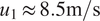
Figure 8 illustrates, on the left, the evolution of the cost function over the optimization iterations for both the upstream (first row) and downstream (second row) wind turbines using all the training episodes. The optimization clearly reduces both cost functions, thus improving the initial guesses from Equation (3.7). Convergence is achieved within a relatively small number of episodes, highlighting the efficiency of the ADAM optimizer with the adjoint-based gradient computation. In the center, Figure 8 shows the power coefficient curves obtained using the initial guesses for the optimization derived from Equation (3.7), based on training grids of
$ {n}_{\lambda_1}\times {n}_{Re} $
 and
$ {n}_{\lambda_2}\times {n}_{\lambda_1} $
and
$ {n}_{\lambda_2}\times {n}_{\lambda_1} $
 samples (indicated by red markers) in the
$ \left({\lambda}_1-\mathit{\operatorname{Re}}\right) $
samples (indicated by red markers) in the
$ \left({\lambda}_1-\mathit{\operatorname{Re}}\right) $
 and
$ \left({\lambda}_2-{\lambda}_1\right) $
and
$ \left({\lambda}_2-{\lambda}_1\right) $
 planes (as described in Section 3.1). These training samples were selected to cover, as broadly as possible, the physical operating space of both wind turbines.
Evolution of the optimization cost functions (left), initial guesses and training data (center), and optimized models (right) for the power coefficients of the upstream (top row) and downstream (bottom row) wind turbines. The red markers in the center plots represent the steady-state training data points used to obtain the initial guesses for the optimization, whereas in the right plots they correspond to trajectories encountered during the training test cases. Similarly, the black markers represent trajectories encountered during the testing cases.
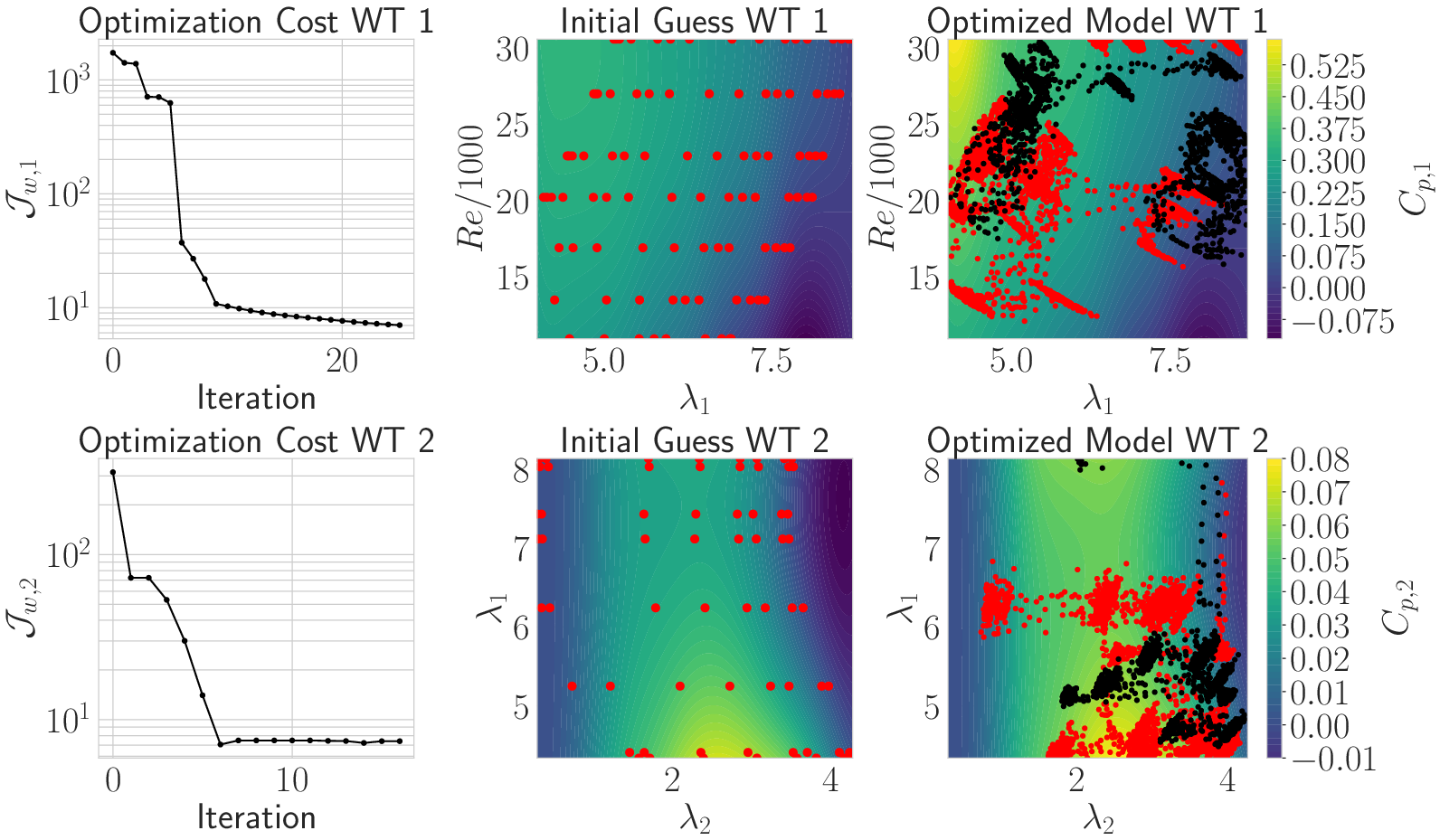
Figure 8. Long description
The multiplot consists of two rows and three columns. The top row corresponds to the upstream wind turbine (WT 1), and the bottom row to the downstream wind turbine (WT 2). In the first column, line graphs plot optimization cost J sub w,1 and J sub w,2 on the y-axis (logarithmic scale) versus iteration on the x-axis, both showing a steep initial decrease followed by a plateau. The middle column contains contour plots of initial guesses for the power coefficient C sub p,1 and C sub p,2, with axes labeled lambda sub 1 and Re all over 1000 for WT 1, and lambda sub 2 and lambda sub 1 for WT 2. Red markers indicate steady-state training data points. The third column presents optimized model contour plots for C sub p,1 and C sub p,2, with the same axes as the middle column. Red markers show training trajectories, and black markers show testing trajectories. Color bars to the right of each contour plot indicate the value range for C sub p,1 (from negative 0.075 to 0.525) and C sub p,2 (from negative 0.01 to 0.08).
On the right, Figure 8 presents the final 2D regressions of the power coefficients: for the first turbine (top), as a function of tip-speed ratio and Reynolds number, and for the second turbine (bottom), as a function of the two tip-speed ratios. The scatter points show the states visited in the training dataset (red markers) and in the testing dataset (black markers). Overall, these provide good coverage, except in the region of low
$ {\lambda}_1 $
 and high
$ \mathit{\operatorname{Re}} $
and high
$ \mathit{\operatorname{Re}} $
 for the first turbine, and in the regions of (i) high
$ {\lambda}_1 $
for the first turbine, and in the regions of (i) high
$ {\lambda}_1 $
 and (ii) simultaneously low
$ {\lambda}_1 $
and (ii) simultaneously low
$ {\lambda}_1 $
 and low
$ {\lambda}_2 $
and low
$ {\lambda}_2 $
 for the second turbine. For the upstream turbine, this gap in the training data results in a nonphysical model in the unsampled region, highlighting the importance of covering a broad range of operating conditions during training. However, considering that the physical system is unable to reach these conditions (e.g.,
$ {\lambda}_1\approx 4 $
for the second turbine. For the upstream turbine, this gap in the training data results in a nonphysical model in the unsampled region, highlighting the importance of covering a broad range of operating conditions during training. However, considering that the physical system is unable to reach these conditions (e.g.,
$ {\lambda}_1\approx 4 $
 with
$ \mathit{\operatorname{Re}}\approx 30000 $
with
$ \mathit{\operatorname{Re}}\approx 30000 $
 ) because of physical limitations, the lack of model accuracy in this area is inconsequential for both predictive and control purposes. For optimization purposes, the model should only be used within the physically admissible operating domain, and the search for the maximum power point should therefore be constrained accordingly. It is worth stressing that the optimized curves do not necessarily reflect the true aerodynamic characteristics of the turbines but rather serve as surrogate models that best reproduce the experimental data, potentially absorbing effects such as measurement noise, generator model errors, or parameter uncertainties (e.g., from CAD estimates).
Figures 9 and 10 show the time evolution of the measured rotational speed of the wind turbines,
$ {\omega}_i^{\ast }(t) $
 , represented in black, along with the associated 95% confidence interval (gray shaded area), and the corresponding predictions of the adaptive models. For both the upstream and downstream turbines, we report the model prediction obtained using the optimal solution, shown with a continuous line, and the model prediction using the initial guess for the model coefficients, shown with dashed lines. In addition, for the upstream turbine only, the prediction obtained from the BEM-based model is also reported (blue dash-dotted line). Each figure presents three randomly selected training trajectories and two test trajectories for both turbines, selected from the pool of available training and testing datasets. The adaptive model demonstrates good agreement with the measured trajectories for both turbines, although predictive performances are slightly lower for the waked turbine, particularly in the description of fluctuation at higher frequencies. This can be attributed to two main factors: (1) reduced coherence between the signals at higher frequencies, and (2) the low-pass filtering effect of the identification procedure, which prioritizes the reconstruction of larger-scale variations.
Time evolution of the measured rotational speed of the upstream wind turbine,
$ {\omega}_1^{\ast }(t) $
 (black line with 95% confidence interval in gray), compared with the predictions from the adaptive models. The solid red line represents the prediction using the optimal solution (
$ {\omega}_1\left(t;{\mathbf{w}}_1\right) $
(black line with 95% confidence interval in gray), compared with the predictions from the adaptive models. The solid red line represents the prediction using the optimal solution (
$ {\omega}_1\left(t;{\mathbf{w}}_1\right) $
 ), the red dotted line shows the prediction from the initial guess model (
$ {\omega}_1\left(t;{\mathbf{w}}_{1,0}\right) $
), the red dotted line shows the prediction from the initial guess model (
$ {\omega}_1\left(t;{\mathbf{w}}_{1,0}\right) $
 ), and the blue dash-dotted line corresponds to the prediction obtained from the BEM-based model (
$ {\omega}_1\left(t;{\boldsymbol{w}}_1^{\mathrm{BEM}}\right) $
), and the blue dash-dotted line corresponds to the prediction obtained from the BEM-based model (
$ {\omega}_1\left(t;{\boldsymbol{w}}_1^{\mathrm{BEM}}\right) $
 ).
).

Figure 9. Long description
From top to bottom, each panel shows omega sub 1 in radians per second versus t in seconds. The top three panels are labeled Training Case 1, Training Case 2, and Training Case 3. The bottom two are Testing Case 1 and Testing Case 2. In all panels, the black dashed line with gray shading shows experimental data with a 95 percent confidence interval. The solid red line represents the optimized model prediction, the red dotted line is the initial guess model, and the blue dash-dotted line is the B E M model. In Training Case 1, the experimental data shows a step increase around t equals 17 seconds, closely followed by the optimized model, while the initial guess and B E M models deviate downward. In Training Case 2 and 3, the optimized model tracks the experimental data, while the initial guess and B E M models underestimate the speed, especially after t equals 10 seconds. In Testing Case 1, a sharp drop in experimental speed at t equals 18 seconds is captured by the optimized model but not by the other models. In Testing Case 2, the optimized model again closely follows the experimental trend, while the initial guess and B E M models remain lower. The legend in the top panel identifies all line styles and colors.
Time evolution of the measured rotational speed of the downstream wind turbine,
$ {\omega}_2^{\ast }(t) $
 (black line with 95% confidence interval in gray), compared with the predictions from the adaptive models. The solid red line represents the prediction using the optimal solution (
$ {\omega}_2\left(t;{\mathbf{w}}_2\right) $
(black line with 95% confidence interval in gray), compared with the predictions from the adaptive models. The solid red line represents the prediction using the optimal solution (
$ {\omega}_2\left(t;{\mathbf{w}}_2\right) $
 ), while the red dotted line shows the prediction from the initial guess model (
$ {\omega}_2\left(t;{\mathbf{w}}_{2,0}\right) $
), while the red dotted line shows the prediction from the initial guess model (
$ {\omega}_2\left(t;{\mathbf{w}}_{2,0}\right) $
 ).
).

Figure 10. Long description
From top to bottom, each panel shows rotational speed omega sub 2 in radians per second on the y axis versus time t in seconds on the x axis. The first three panels are labeled Training Case 1, Training Case 2, and Training Case 3. The bottom two panels are labeled Testing Case 1 and Testing Case 2. In each panel, a black dashed line represents experimental data, with a surrounding gray band indicating the 95 percent confidence interval. A solid red line shows the optimized model prediction, and a red dotted line shows the initial guess model. The legend appears in the top panel. Across all panels, the optimized model closely tracks the experimental data, especially during rapid increases and decreases in rotational speed, while the initial guess model consistently underestimates the speed and lags behind the experimental trend. The x axis ranges from 0 to 30 seconds in all panels, and the y axis ranges from 100 to 300 radians per second, with minor variations in minimum and maximum values depending on the panel.
For the upstream turbine, the BEM-based model shows the poorest agreement among the considered models, with larger deviations from the measurements across several test cases. Moreover, the comparison between the initial and optimized models shows that the main improvement lies in a significantly better representation of the system’s stability properties. In some cases (Training Cases 2, 3, and Testing Case 2 for the upstream turbine), the initial parameter guess from Equation (3.7) leads the model to be undesirably and unrealistically attracted to the fixed point
$ \omega =0 $
 , resulting in shutdown-like behavior that does not match the collected data (see also Section 3.3). On a practical note, we emphasize that the cost function exhibits significant stiffness in regions of the parameter space where changes in stability properties occur. To help the ADAM optimizer adapt to these abrupt changes, we reinitialize it whenever a threshold is crossed (
$ \Delta {\mathcal{J}}_{w,i}>100 $
, resulting in shutdown-like behavior that does not match the collected data (see also Section 3.3). On a practical note, we emphasize that the cost function exhibits significant stiffness in regions of the parameter space where changes in stability properties occur. To help the ADAM optimizer adapt to these abrupt changes, we reinitialize it whenever a threshold is crossed (
$ \Delta {\mathcal{J}}_{w,i}>100 $
 ), effectively restarting the gradient smoothing procedure in Equation (3.16). This re-initialization occurs, for instance, between iterations 3–4 and 6–7 in the upstream turbine case, as shown in the cost function evolution in Figure 8. Additionally, we observe that once the cost function falls below a small threshold (
$ {\mathcal{J}}_{w,i}<10 $
), effectively restarting the gradient smoothing procedure in Equation (3.16). This re-initialization occurs, for instance, between iterations 3–4 and 6–7 in the upstream turbine case, as shown in the cost function evolution in Figure 8. Additionally, we observe that once the cost function falls below a small threshold (
$ {\mathcal{J}}_{w,i}<10 $
 ), the momentum term becomes detrimental to convergence. In such cases, reducing the learning rate by a factor of 10 improves convergence by enabling finer adjustments in promising regions of the parameter space.
5.2. Identification in high turbulence
As in the previous section, we begin by analyzing the correlation between the normalized incoming velocity
$ {\hat{u}}_1(t) $
 and the rotational speed of the upstream turbine
$ {\hat{\omega}}_1(t) $
and the rotational speed of the upstream turbine
$ {\hat{\omega}}_1(t) $
 , shown in Figure 11. This test case corresponds to stationary conditions with high turbulence, where wind speed fluctuates between 7 and 11 m/s. As a consequence that the velocity measurement is not taken at the hub of the turbine, the variables
$ {u}_1(t) $
, shown in Figure 11. This test case corresponds to stationary conditions with high turbulence, where wind speed fluctuates between 7 and 11 m/s. As a consequence that the velocity measurement is not taken at the hub of the turbine, the variables
$ {u}_1(t) $
 and
$ {\omega}_1(t) $
and
$ {\omega}_1(t) $
 exhibit no meaningful correlation, meaning that it is impossible to reconstruct the turbine’s rotational speed time series as done in the previous case. Nonetheless, the objective here is to capture the time-averaged signal, even in the absence of short-term correlation. Although short-term inflow–response correlation is reduced, the model captures the dominant fluctuations occurring over larger temporal scales, which remain relevant for control-oriented applications.
Left: Time evolution of the dimensionless wind speed at the location highlighted in Figure 6 (
$ {\hat{u}}_1 $
 ) and the dimensionless rotational speed of the first turbine (
$ {\hat{\omega}}_1 $
) and the dimensionless rotational speed of the first turbine (
$ {\hat{\omega}}_1 $
 ). Right: Scatter plot showing the low correlation inflow conditions and turbine dynamics.

Figure 11. Long description
The left panel is a line graph with x-axis labeled t in seconds and y-axis labeled Scaled states. Two overlaid lines are shown: a blue line for u sub 1 hat and a brown line for omega sub 1 hat, both fluctuating between minus 0.5 and 0.5 over a time span from 0 to 100 seconds. The legend in the upper left identifies the blue line as u sub 1 hat and the brown line as omega sub 1 hat. The right panel is a scatter plot with x-axis labeled u sub 1 hat and y-axis labeled omega sub 1 hat, both ranging from minus 0.5 to 0.5. Blue points are scattered with no clear trend. A dashed black line labeled y equals x runs diagonally from bottom left to top right, indicating the line of perfect correlation. The scatter shows low correlation between the two variables.
Figure 12 (top) presents the sampled pairs
$ \mathit{\operatorname{Re}}-{\lambda}_1 $
 for the first (upstream) turbine and
$ {\lambda}_i-{\lambda}_{i+1} $
for the first (upstream) turbine and
$ {\lambda}_i-{\lambda}_{i+1} $
 for the downstream (waked) turbines. Samples from the training and test phases are indicated with red and black markers, respectively, while the blue markers represent the states visited by the model when attempting to track the test cases. The orange star indicates the mean value. The dashed line shows the direction of the leading principal component in the sample space.
Summary of the identification result for the wind farm scenario under highly turbulent conditions. The first row shows the location of the sampling and testing points for the three turbines (refer to Figure 6 for their position). The second row shows the power coefficient curves obtained from the initial guess and the optimized weights for the high-turbulence scenario, as well as those corresponding to the low-turbulence scenario. In the bottom-left panel, the low-turbulence optimized model for the first turbine, evaluated under high-turbulence conditions, is displayed only within the physically meaningful range.

Figure 12. Long description
There are six panels arranged in two rows and three columns. The top row contains scatter plots for Wind Turbine 1, Wind Turbine 2, and Wind Turbine 3, from left to right. Each scatter plot shows two distributions: red points for training data and blue points for testing data. The x-axis for Wind Turbine 1 is labeled lambda sub 1, and the y-axis is R e times 10 to the minus 3. For Wind Turbine 2, the x-axis is lambda sub 1 and the y-axis is also lambda sub 1. For Wind Turbine 3, both axes are labeled lambda sub 2. All three plots include a dashed diagonal line and a yellow cross marking a central point. The bottom row contains line graphs of power coefficient C sub p versus lambda for each turbine. The leftmost plot shows C sub p,1 versus lambda sub 1, the center plot shows C sub p,2 versus lambda sub 2, and the rightmost plot shows C sub p,3 versus lambda sub 3. Each line graph includes three curves: a blue dashed line for C sub p guess, an orange solid line for optimized high turbulence, and a green dash-dot line for optimized low turbulence. The center bottom panel includes a legend. The leftmost bottom panel is restricted to the physically meaningful range for the first turbine under high turbulence.
Two main observations arise. First, although the model does not perfectly reproduce the instantaneous values, the predictions remain well within the distribution of the observed data, with the mean value largely preserved. Second, the correlation in the sample space is significantly higher for the waked turbines compared to the upstream one. This suggests that, in terms of input/output behavior, the wind farm acts as a low-pass filter on the incoming turbulence.
Figure 12 (bottom) shows the predicted power coefficient along the principal component of the sampled space, comparing the initial guess, the optimized solution obtained from the high-turbulence dataset, and the optimized model previously trained in the low-turbulence scenario and then tested in the present high-turbulence case. In this case, only the physically meaningful range is displayed, as the extrapolated region is associated with non-physical values. The observed discrepancy in performance across the three turbines is expected, as wake effects lead to notably lower power coefficients in the downstream turbines. The substantial difference between the initial and optimized predictions in the high-turbulence case indicates that the optimization significantly modifies the identified model. Its effect is better assessed through comparison with the experimental data discussed later in Figure 13. Of particular interest is the sensitivity of the upstream turbine’s power curve to turbulence intensity: high-frequency fluctuations are filtered out by the turbine dynamics, and thus a model trained in low-turbulence conditions, mainly influenced by large-scale fluctuations, tends to yield overly optimistic and potentially nonphysical predictions. Conversely, for the waked turbines, turbulence enhances wake recovery, although only slightly under these conditions, as the increase in the power coefficient relative to the initial guess in the low-turbulence scenario is modest. Consequently, models trained under high-turbulence conditions yield more accurate predictions than those trained in calm flows.
Model assimilation results for the three wind turbine models under high-turbulence conditions, using the testing dataset. The continuous red lines represent the adaptive model predictions
$ {\omega}_i\left(t;{\mathbf{w}}_i\right) $
 , the black lines correspond to the experimental data
$ {\omega}_i^{\ast }(t) $
, the black lines correspond to the experimental data
$ {\omega}_i^{\ast }(t) $
 , and the gray shaded bands indicate the associated measurement uncertainty (95% confidence interval). The initial-guess predictions are shown as red dotted lines
$ {\omega}_i\left(t;{\mathbf{w}}_{i,0}\right) $
, and the gray shaded bands indicate the associated measurement uncertainty (95% confidence interval). The initial-guess predictions are shown as red dotted lines
$ {\omega}_i\left(t;{\mathbf{w}}_{i,0}\right) $
 , while the BEM-based predictions for the first turbine are included in blue as dashed-dotted lines
$ {\omega}_1\left(t;{\boldsymbol{w}}_1^{\mathrm{BEM}}\right) $
, while the BEM-based predictions for the first turbine are included in blue as dashed-dotted lines
$ {\omega}_1\left(t;{\boldsymbol{w}}_1^{\mathrm{BEM}}\right) $
 . The plot highlights the substantial fluctuations in rotational speed caused by high turbulence, as well as the inherent limitations of the adaptive model in fully capturing the instantaneous dynamics. Nevertheless, the model successfully reproduces the mean and standard deviation of the waked turbines, whereas the standard deviation of the first turbine is represented with lower accuracy, as evidenced by the probability density function (PDF) distributions shown in the plots on the right.

Figure 13. Long description
The visualization is organized into three horizontal panels, each corresponding to a different wind turbine, labeled Wind Turbine 1 at the top, Wind Turbine 2 in the middle, and Wind Turbine 3 at the bottom. In each panel, the x-axis represents time in seconds, ranging from 0 to 25, and the y-axis represents rotational speed omega sub i in radians per second. The left side of each panel displays time series data: black dashed lines show experimental measurements, gray shaded bands indicate the 95 percent confidence interval for measurement uncertainty, solid red lines represent adaptive model predictions, red dashed lines show initial guess predictions, and in the top panel only, blue dash-dotted lines display B E M-based predictions. The legend at the top of the first panel identifies each line style and color. On the right of each panel, a probability density function plot compares the distribution of rotational speeds for each data series, with matching colors and line styles. The experimental and model distributions are closely aligned for turbines 2 and 3, but the model underestimates the standard deviation for turbine 1, as seen by the narrower red distribution compared to the black. The time series plots reveal substantial fluctuations in rotational speed due to high turbulence, with the adaptive model capturing the mean and standard deviation for the waked turbines but not for the first turbine.
Regarding the shape of the identified power coefficient curves, it is important to consider the sample distribution used for model identification. For example, the apparent double-peaked shape in the upstream turbine’s power curve is likely nonphysical and results from insufficient data in the regions
$ {\lambda}_1<4 $
 and
$ {\lambda}_1>6 $
and
$ {\lambda}_1>6 $
 . However, since these operating conditions are rarely visited, this has little impact on the model’s predictive performance. Overall, the strong sensitivity of the identified performance curves to the turbulence conditions in the training data underscores the value of continuously adapting the model over the turbine’s operational life. This aligns well with the proposed episodic system identification framework, where the model is not trained once for all but is periodically updated in episodes, each time incorporating newly observed operational data to improve accuracy and robustness.
Finally, Figure 13 shows the model predictions and measured rotational speeds for all three turbines in the test dataset. As in the previous figures, adaptive model predictions are shown as continuous red lines, experimental measurements in black, and the associated uncertainty as a gray confidence band. In addition, red dotted lines show the prediction of the initial guess obtained from Equation (3.7), while for the first turbine only, BEM predictions are shown in dashed-dotted line in blue. The high turbulence environment results in substantial fluctuations in rotational speed across all turbines. For each case, the right panel presents the probability density function (PDF) of the measured data and that predicted by the optimized model. In all cases, the mean is accurately captured by the final optimized model, while the standard deviation is slightly underestimated for the upstream turbine, likely due to the weaker input–output correlation in the training data (see Figure 12, top left). By contrast, for the first wind turbine, both the BEM model and the initial-guess model do not accurately capture the mean. However, they provide a better estimate of the standard deviation. This behavior is likely due to the smoother shape of the corresponding power coefficient, whereas the optimized model exhibits this double-peaked structure, which may affect the representation of the variability. Interestingly, the model reconstructs the distributions more accurately for the waked turbines. These results indicate that, under high-turbulence conditions, the model accurately reproduces the statistical behavior of the turbine response, while high-frequency fluctuations are not fully resolved.
5.3. Control performance from identified models
The identified model is integrated in the
$ K{\omega}^2 $
 control law as described in 4.4 for both the upstream and downstream turbine in the low turbulence scenario. The control challenge consists in keeping a reference trajectory in terms of tip-speed ratio, hence define a time varying reference
$ \lambda $
control law as described in 4.4 for both the upstream and downstream turbine in the low turbulence scenario. The control challenge consists in keeping a reference trajectory in terms of tip-speed ratio, hence define a time varying reference
$ \lambda $
 (and associated power coefficient) in Equation (4.3) rather than the power maximization. This choice was made to assess the controller performance over a broader portion of the operating domain, instead of restricting the analysis to a single maximum-power operating condition. Such a formulation is also relevant in view of wind-farm control, where the optimal set-point of each turbine may differ from its individual maximum-power point.
The results for the upstream turbine are shown in Figure 14. The top plot displays the dynamic set point alongside the actual tip-speed ratio for three controllers based on different models: (1) the blade element momentum (BEM)-regressed model (green), (2) the initial guess power coefficient curve assuming steady-state conditions (orange), and (3) the adapted model obtained after the identification process (blue). The middle plot shows the control action, i.e., the variation in generator resistance applied by each controller, while the bottom plot presents the incoming wind velocity during the three control tests, which remained relatively similar. It is worth noting that the large variations in set point were not intended to mimic a realistic control task—which would typically aim to track the optimal power coefficient—but were instead designed to stress-test the controllers.
Test of the adaptive model of the upstream turbine in the low turbulence scenario using the
$ K{\omega}^2 $
 control law. The setpoint in terms of tip speed ratio is highlighted in red. The controller using the adaptive model (blue) is compared with the controller using the model obtained through BEM simulations (green) and steady-state data regression used as an initial guess for the optimization (orange). It can be seen that the controller with the adaptive model outperforms the others.

Figure 14. Long description
The top panel plots tip speed ratio lambda sub 1 on the y-axis versus time t in seconds on the x-axis. Four traces are shown: blue for optimized, orange dashed for initial guess, green dash-dot for B E M, and red dotted for setpoint. All traces rise rapidly to near the setpoint, with the blue optimized trace closely following the red setpoint, especially after t equals 25 seconds, while the green and orange traces deviate more. The middle panel plots R sub van in ohms versus time. The blue optimized and orange initial guess traces drop sharply after t equals zero, remain low, then step up after t equals 25 seconds, with the blue trace stabilizing lower than the others. The green B E M trace remains higher throughout. The bottom panel plots v sub inflow in meters per second versus time. All traces fluctuate around 4.1 meters per second, with the blue optimized trace showing the least variation. The legend at the top left identifies each trace by color and line style.
The superior performance of the controller driven by the adapted model, as compared to the BEM-driven controller, is evident. The large steady-state errors and excessive actuation observed with the BEM-driven controller can be attributed to model deficiencies, which are already apparent from the comparison in Figure 9 and are likely related to the uncertain prediction of low-Reynolds-number effects. Although these could be corrected by more sophisticated control laws, it is interesting to note that the adaptive formulation yields excellent tracking performances with the simplest
$ K{\omega}^2 $
 controller.
The difference in control performances of the initial and adapted model appears minor in comparison. After all, as described in the previous section, the initial guess yields overall satisfactory models as long as the stability properties are preserved. Nevertheless, the difference is appreciable. Considering the impact of power curve modeling on energy production (Pao and Johnson, Reference Pao and Johnson2009), and considering that wind turbine dynamics change over their lifespan due to factors such as mechanical wear, environmental conditions, and blade fouling, the ability to adapt and refine the model remains essential for maintaining optimal performance and long-term efficiency.
Finally, a similar analysis is presented for the waked turbine in Figure 15, a scenario well beyond the reach of traditional modeling approaches due to strong inflow unsteadiness and limited flow characterization. Time-dependent set points are prescribed for both turbines. The top plot shows the tracking performance of the upstream turbine, while the second plot presents the response of the downstream turbine, alongside an uncontrolled baseline scenario. The uncontrolled response clearly reveals the wake effect on the second turbine when the upstream set point
$ {\lambda}_1 $
 is changed at
$ t=25 $
is changed at
$ t=25 $
 s and
$ t=50 $
s and
$ t=50 $
 s. The third plot shows the control input, with a visible actuation step triggered by the set point change, as well as the downstream response to upstream variation.
Test of the adaptive models of the tandem configuration in the low turbulence scenario with the
$ K{\omega}^2 $
 control law. Both the first wind turbine and the downstream turbine are controlled to follow a determined setpoint highlighted in red. A comparison with the uncontrolled case of the downstream turbine (orange) is presented. In this scenario, the effect of the wake is clearly visible, as is the corrective action applied by the controller to the downstream turbine to counteract this effect.

Figure 15. Long description
The top panel plots lambda sub 1 on the y-axis from 4 to 7 against time t in seconds from 0 to 65. The blue solid line labeled Control closely tracks the red dotted Setpoint line, both showing step increases at approximately t equals 0, 20, and 50 seconds. The middle panel plots lambda sub 2 from 1 to 3. The blue solid Control line follows the red dotted Setpoint with step changes at the same times as above, while the orange dashed No control line remains consistently lower and does not track the setpoint. The bottom panel plots R sub 2 opt in ohms on a logarithmic scale from 1 to 10, showing the blue line with step increases at the same time points, corresponding to the setpoint changes. Legends in the top and middle panels identify Control, No control, and Setpoint lines. All axes are labeled with their respective variables and units.
The key result is highlighted in the second plot: the controller, based on the identified model, successfully mitigates the impact of upstream disturbances (at
$ t=25 $
 s and
$ t=50 $
s and
$ t=50 $
 s) and accurately tracks the reference step change (at
$ t=32 $
s) and accurately tracks the reference step change (at
$ t=32 $
 s). Although some oscillations appear in the controlled
$ {\lambda}_2 $
s). Although some oscillations appear in the controlled
$ {\lambda}_2 $
 signal, the overall results demonstrate excellent tracking and disturbance rejection performance within the model bandwidth, even in the presence of wake-induced disturbances. These oscillations can be attributed to an inherent limitation of the
$ K{\omega}^2 $
signal, the overall results demonstrate excellent tracking and disturbance rejection performance within the model bandwidth, even in the presence of wake-induced disturbances. These oscillations can be attributed to an inherent limitation of the
$ K{\omega}^2 $
 controller, which, by design, assumes steady-state operating conditions (see Pao and Johnson, Reference Pao and Johnson2009) and lacks feedback control command from the incoming wind velocity. Consequently, its tracking performances degrade under rapidly changing wind conditions because changes in wind velocity are only sensed via changes in rotor speed, which are lagged due to inertia. This limitation is visible for the waked turbine but not for the upstream one, which operates in low turbulence and slow variations of the wind speed.
6. Conclusions
In this work, we proposed and experimentally validated a system identification approach for free-stream and waked wind turbines based on the online estimation of nonlinear power coefficient curves. By combining compactly supported radial basis functions with low-order polynomial regressors, the method yields physically interpretable surrogate representations of turbine performance suitable for control-oriented dynamic models. The methodology was tested on both low- and high-turbulence scenarios using small-scale wind turbines. In the low-turbulence case, the identified models showed strong agreement with the experimental measurements. In the high-turbulence case, although the instantaneous dynamics were not fully reproduced, the models were able to capture the main statistical features of the turbine response despite the unresolved turbulent fluctuations.
The adaptive models were successfully integrated into the
$ K{\omega}^2 $
 controller, demonstrating enhanced performance over conventional control strategies based on BEM or steady-state regressions. In a controlled tandem configuration, the adaptive controllers were able to mitigate wake-induced effects on a downstream turbine, validating the potential of this framework for coordinated wind farm operation. Moreover, the ability of the model to adapt to different operating regimes, including noisy and turbulent conditions, supports its practical applicability. In these conditions, the model captures the statistical and low-frequency behavior of the turbine response, while finer-scale fluctuations remain outside the scope of the present formulation. The proposed identification process, based on adjoint gradient computation and ADAM optimization, enables adaptability while remaining computationally efficient. Importantly, the resulting models retain a structure that is compatible with existing model-based industrial controllers, potentially allowing their integration without major architectural modifications.
Future developments could explore the integration of this adaptive modeling approach into more advanced control strategies such as model predictive control (MPC). At full scale, the proposed framework could use episodic online model updating with the same inputs as the current method: standard SCADA signals and a farm-level freestream velocity estimate, for example from lidar. A practical path is to first identify turbine-specific surrogate power-coefficient models offline to provide an initial guess, then periodically update them during operation to reflect wake interactions, turbulence, and performance degradation from aging or blade surface changes. At the wind-farm level, these updated models could be integrated into existing supervisory or model-based controllers to improve set-point coordination, wake mitigation, and energy capture without redesigning the control architecture.
Despite the promising potential and the implementation pathway outlined above, intermediate steps are still needed before the proposed methodology can be deployed at full scale. This study considers a simplified configuration, with turbines aligned with the incoming flow and operating under controlled inflow. Although the data-driven formulation implicitly captures some unsteady and turbulent effects in the identified power coefficient, additional real wind farm complexities such as yaw misalignment, time-varying wind direction and terrain-induced flow heterogeneity should be included.
Acknowledgements
The authors gratefully acknowledge the contribution of Jacquet Charles, who worked on the farm testing in the framework of his research master project. The authors also acknowledge the use of AI-based tools to assist in improving the clarity, grammar, and overall readability of the manuscript. All ideas, analyses, results, and scientific content are original and were entirely conceived and developed by the authors.
Data availability statement
The experimental data supporting the findings of this study are openly available in Zenodo (Randino, Reference Randino2026) at https://doi.org/10.5281/zenodo.19631347.
Author contribution
Conceptualization: S.R. and M.A.M. Methodology: S.R., L.S., N.C., and M.A.M. Investigation: S.R. and M.A.M. Software: S.R. Data curation: S.R. Resources: M.A.M. Writing – original draft: S.R. Writing – review & editing: L.S., N.C., and M.A.M. Supervision: L.S., E.G., and M.A.M. Project administration: M.A.M. Funding acquisition: M.A.M. All authors approved the final submitted draft.
Funding statement
This research was initially developed as part of the research master’s project of Sebastiano Randino, supported by a VKI NATO Fellowship. It was subsequently refined and extended during the PhD work of Sebastiano Randino, funded by a FNRS FRIA Fellowship (Fellowship number 40029825). Lorenzo Schena is funded by an FWO Fellowship (number 1567925 N). This work is also part of the RE-TWIST project, which has received funding from the European Research Council (ERC) under the European Union’s Horizon Europe programme (grant agreement No 101165479). The views expressed are those of the authors and do not necessarily reflect those of the European Union or the ERC.
Competing interest
The authors declare that they have no known competing financial interests or personal relationships that could have appeared to influence the work reported in this paper.


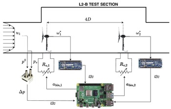


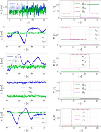

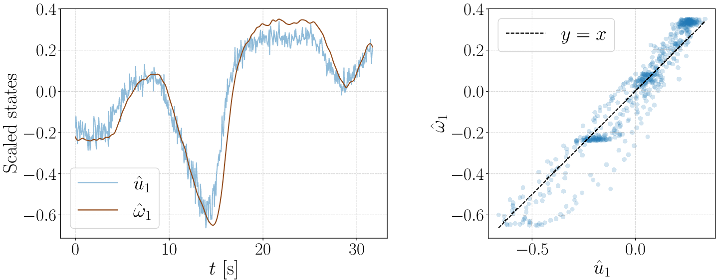


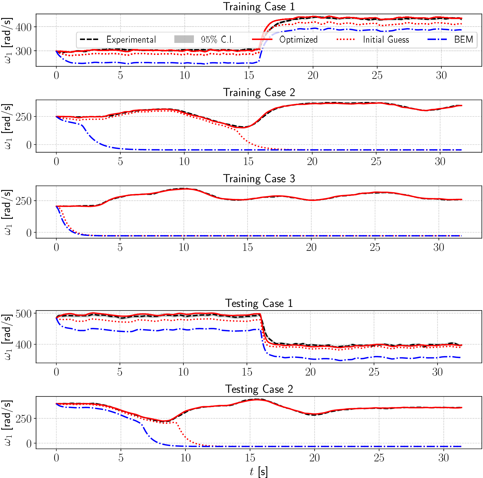


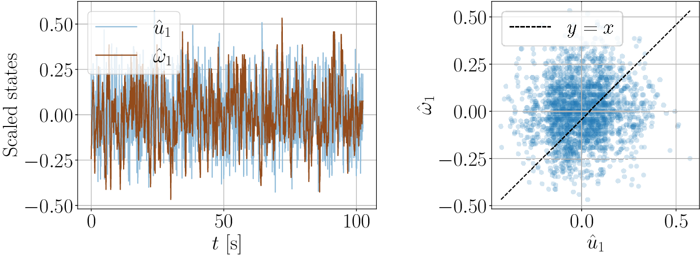


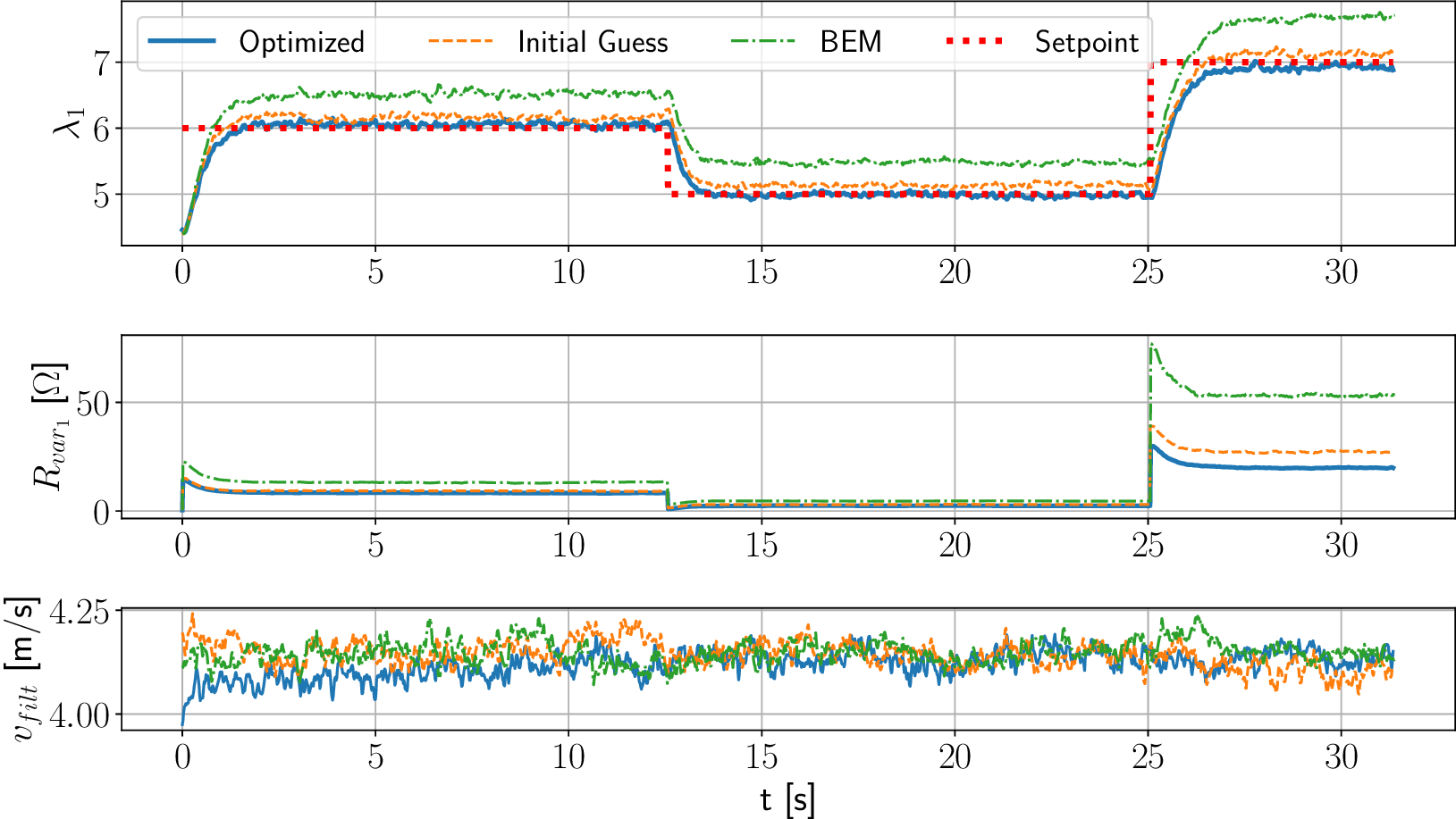

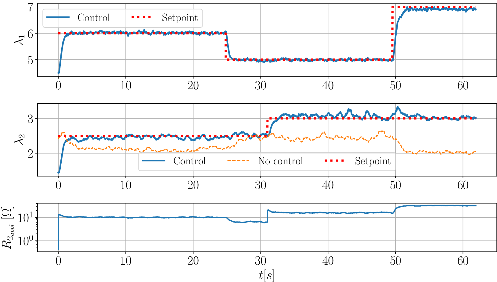


 Open access
Comments
No Comments have been published for this article.