


Impact Statement
Deep learning methods have been increasingly developed and utilized in making critical predictions in complex engineering problems. A new category of such methods incorporates some physical insight (e.g., conservation laws) in their architectures, in order to guide the training of the deep learning models and improve their accuracy. A similar approach is followed in the present study, focusing on the AI modeling of traveling droplets over a chemically heterogeneous surface, which is a type of flow that is of interest across a broad spectrum of technological areas such as microfabrication, biomedicine, and energy applications among others. More specifically, the best-performing model in the present study uses an analytically derived, albeit imperfect model as the base solution, upon which corrections are introduced in a data-driven manner. This approach is demonstrated to accurately capture the dynamics, even for surface profiles that are significantly different from the ones used to train the data-driven model. Adopting such an AI-assisted approach holds the potential to significantly reduce the solution time compared to computationally intensive high-fidelity simulations, expediting also the design of surface features for controllable droplet transport. This approach, which is being applied for the first time in the context of contact line dynamics, constitutes a proof-of-concept that may be extended in different settings beyond contact line motion.
1. Introduction
Wetting hydrodynamics concerns the dynamics of liquids in contact with surfaces and entails multi-physics processes that operate at disparate scales. Central to this class phenomena is the motion of the contact line, which is formed at the junction where typically liquid, gas, and solid phases meet. Depending on the level of detail at which the dynamics are resolved, this can often pose formidable large-scale computing challenges. These challenges are often overcome by resorting to low-fidelity models which typically rely on empirical approximations to capture unresolved physics. However, this limited predictive capability is not desirable in applications of practical importance, where the need to precisely control how a liquid behaves when deposited on a surface is key. These challenges are highly relevant to a broad spectrum of scientific and technological areas, including, to name a few, microfabrication, smart materials, biomedicine, pharmaceutical and printing industries, as well as energy conversion and water harvesting in environmental applications (see, e.g., Bonn et al., Reference Bonn, Eggers, Indekeu, Meunier and Rolley2009, for a review). Thus, in order to address the need for accurate and efficient data generation in these settings, deep learning approaches emerge as a promising alternative to high-fidelity simulations.
In the broader context of fluid dynamics, the uptake of deep learning methodologies has been overwhelming in the past few years, mainly due to the abundance of data generated from experimental and numerical studies, the evolution of hardware, especially in graphics processing units (GPUs), and the broad availability of efficient open source frameworks and algorithms (Brunton et al., Reference Brunton, Noack and Koumoutsakos2020; Vinuesa and Brunton, Reference Vinuesa and Brunton2021). Some illustrative examples of areas in fluid dynamics where deep learning approaches are being used include, among others, turbulence modeling (Ahmed et al., Reference Ahmed, Pawar, San, Rasheed, Iliescu and Noack2021), reduced-order models for extracting dominant coherent structures (Lee and Carlberg, Reference Lee and Carlberg2020), nonintrusive sensing (Guastoni et al., Reference Guastoni, Güemes, Ianiro, Discetti, Schlatter, Azizpour and Vinuesa2021). In contrast, the adoption of deep learning in multi-phase flows is not as widespread, with many open questions and opportunities for delivering impact (Gibou et al., Reference Gibou, Hyde and Fedkiw2019). Noteworthy here are two works involving multi-phase flows with a deep learning orientation, which study the data-driven prediction of the kinematics of spherical particles (Wan and Sapsis, Reference Wan and Sapsis2018) and bubbles (Wan et al., Reference Wan, Karnakov, Koumoutsakos and Sapsis2020). In these works, imperfect models, which were obtained through analytical arguments and possess a limited regime of applicability, are complemented with a data-driven contribution that is trained to learn the difference between the prediction of the imperfect analytical model and the reference solution. The reported performance of these hybrid models highlights the merits of such an approach, as they were shown to generalize well to more complex cases outside the training datasets. This was achieved without the need to make readjustments to the network parameters, whilst being able to significantly improve the predictions of the pertinent analytical models.
However, the potential of deep learning methods for the study of the dynamics of contact lines as an alternative to computationally expensive simulations has not been previously explored. Hence, this work constitutes a first attempt toward the development of data-driven models that are able to reproduce the dynamics of isolated droplets moving on heterogeneous surfaces. To this end, there is presently a proliferation of candidate deep learning architectures that may be deployed depending on the intended application. Within the context of using neural networks for learning solutions to partial differential equations (PDEs), like the ones considered herein, it is important for such data-driven approaches to be capable of obtaining generalizable models. Such models may then be used for a broad range of parameters and auxiliary data that capture as diverse dynamics as possible, extending beyond the dynamics of the training datasets. This is particularly true when dealing with transport phenomena in the presence of complex heterogeneous environments, where small temporal or spatial errors can lead to markedly different behaviors in the longer term.
One particularly interesting class of such neural network architectures is associated with the concept of the neural operator, as it was shown to be capable of learning resolution-invariant mappings between infinite-dimensional function spaces, in a manner that is able to approximately capture the relationship between the auxiliary data of a PDE (including its parameters, initial and boundary conditions) and the solution, without the need to retrain the model for a new set of auxiliary data (Kovachki et al., Reference Kovachki, Li, Liu, Azizzadenesheli, Bhattacharya, Stuart and Anandkumar2021b; Lu et al., Reference Lu, Jin, Pang, Zhang and Karniadakis2021). A key feature of neural operators is the combination of linear, nonlocal operators with nonlinear, local activation functions. The way these nonlocal operators are represented lies at the heart of neural operator architectures, giving rise to various alternatives, which include, for example, spectral representations, graph neural networks, low-rank kernel decompositions, and fast multipole methods (see, e.g., Kovachki et al., Reference Kovachki, Li, Liu, Azizzadenesheli, Bhattacharya, Stuart and Anandkumar2021b, for an overview). Other classes of deep-learning-based PDE solvers include physics-informed neural networks (PINNs) (Raissi et al., Reference Raissi, Perdikaris and Karniadakis2019), solver-in-the-loop (Um et al., Reference Um, Brand, Yun, Holl and Thuerey2021), and message-passing neural PDE solver (Brandstetter et al., Reference Brandstetter, Worrall and Welling2022), among others.
The present study examines the use of the Fourier neural operator (FNO), originally proposed by Li et al. (Reference Li, Kovachki, Azizzadenesheli, Liu, Bhattacharya, Stuart and Anandkumar2020), which parametrizes the nonlocal operator in the Fourier space. This specific formulation was tested by Li et al. for different PDEs, such as the Burgers and the Navier–Stokes equations and was shown to be competitive against other established deep learning methods such as fully convolutional networks (Zhu and Zabaras, Reference Zhu and Zabaras2018), residual neural networks (He et al., Reference He, Zhang, Ren and Sun2016), U-Nets (Ronneberger et al., Reference Ronneberger, Fischer and Brox2015), and so forth. FNO was also shown to be a subcase of DeepONets (Lu et al., Reference Lu, Jin, Pang, Zhang and Karniadakis2021), which constitute a broader framework for representing neural operator architectures (Kovachki et al., Reference Kovachki, Lanthaler and Mishra2021a). Lu et al. (Reference Lu, Meng, Cai, Mao, Goswami, Zhang and Karniadakis2022) presented a comprehensive comparison between FNO and DeepONet. Both approaches were found to exhibit similar accuracy and performance levels in a range of examples, but FNOs were less flexible than DeepONets in handling complex geometries. More recently, the FNO architecture was extended to better tackle complex geometries as well (Li et al., Reference Li, Huang, Liu and Anandkumar2022). Focusing on the computing cost–accuracy trade-off, De Hoop et al. (Reference De Hoop, Huang, Qian and Stuart2022) concluded that FNOs may be the better choice for one- and two-dimensional problems, but DeepONets are preferable for three-dimensional problems, because the cost of FNOs scales with the dimensionality of the problem. For the problem under investigation, FNOs are arguably the method of choice as they naturally apply to periodic domains, in alignment with the periodicity of the closed contact lines considered herein. Hence, rather than pursuing the route of showing detailed comparisons with other candidate architectures which have already been followed in the aforementioned works (see, e.g., Li et al., Reference Li, Kovachki, Azizzadenesheli, Liu, Bhattacharya, Stuart and Anandkumar2020; De Hoop et al., Reference De Hoop, Huang, Qian and Stuart2022; Lu et al., Reference Lu, Meng, Cai, Mao, Goswami, Zhang and Karniadakis2022), in this work, we examine two alternative uses of FNOs. Both approaches are applied to one-dimensional data derived from the evolution of a contact line, which is parametrized by the azimuthal angle about the centroid position of the contact area.
Training and testing datasets consist of contact line snapshots as a droplet traverses the heterogeneous features of the substrate. Two approaches are presented here, which are evaluated in terms of accuracy and generalizability: in the first (hereinafter referred to as approach A), the FNO is used as an iterative architecture, predicting the solution at fixed time steps based on the history of the system, following similar ideas as those presented in the original contribution on the FNO (Li et al., Reference Li, Kovachki, Azizzadenesheli, Liu, Bhattacharya, Stuart and Anandkumar2020); in the second (referred to as approach B), the FNO augments a less accurate leading-order analytical approximation to the contact line velocity, which is then evolved in time using standard techniques. In this manner, the aim is to improve upon an approximate model, derived from the work of Lacey (Reference Lacey1982), with a data-driven component for capturing higher-order corrections. The second approach is inspired by the asymptotic analyses carried out by Savva et al. (Reference Savva, Groves and Kalliadasis2019) and Savva and Groves (Reference Savva and Groves2021), which have shown that the inclusion of additional terms can indeed considerably improve the agreement with solutions to the governing equation. It is also similar in spirit with other recent contributions, although these were applied in other physical systems and employed different neural network architectures (Wan and Sapsis, Reference Wan and Sapsis2018; Wan et al., Reference Wan, Karnakov, Koumoutsakos and Sapsis2020). An account of the numerical methods used for generating simulation datasets and the training of the data-driven models is presented in Section 2. This is followed by the presentation of the results of the two different approaches in Section 3, summarizing the key findings of the work in Section 4.
2. Methods
This section provides an overview of the mathematical model and the methods used for producing training datasets, alongside with a brief description of the deep learning architecture employed.
2.1. Mathematical model
Studying systems involving moving contact lines requires expensive multiphase and multiscale computational fluid dynamics simulations based on a number of different approaches, the most popular of which being phase field models (see, e.g., Huang et al., Reference Huang, Lin and Ardekani2020; Shahmardi et al., Reference Shahmardi, Rosti, Tammisola and Brandt2021), volume-of-fluid methods (see, e.g., Afkhami et al., Reference Afkhami, Zaleski and Bussmann2009; Popinet, Reference Popinet2009), and the Lattice Boltzmann method for mesoscale problems (see, e.g., Kusumaatmaja and Yeomans, Reference Kusumaatmaja and Yeomans2007; Srivastava et al., Reference Srivastava, Perlekar, Biferale, Sbragaglia, ten Thije Boonkkamp and Toschi2013). In the limit of strong surface tension, negligible inertia, and small contact angles, we may invoke the so-called long-wave theory (Greenspan, Reference Greenspan1978) to deduce a single nonlinear PDE for the evolution of the droplet thickness $ h\left(\boldsymbol{x},t\right) $
as it moves on a horizontal and chemically heterogeneous surface in space
$ h\left(\boldsymbol{x},t\right) $
as it moves on a horizontal and chemically heterogeneous surface in space $ \boldsymbol{x}=\left(x,y\right) $
and time
$ \boldsymbol{x}=\left(x,y\right) $
and time $ t $
, cast in dimensionless form as
$ t $
, cast in dimensionless form as
 $$ {\partial}_th+\mathbf{\nabla}\cdot \left[h\left({h}^2+{\lambda}^2\right)\mathbf{\nabla}{\nabla}^2h\right]=0, $$
where $ \lambda $
is the slip length that is used to relax the stress singularity that would occur at a moving contact line with the classical no-slip boundary condition (Huh and Scriven, Reference Huh and Scriven1971). Equation (1a) is made nondimensional by scaling the lateral scales with
$ \lambda $
is the slip length that is used to relax the stress singularity that would occur at a moving contact line with the classical no-slip boundary condition (Huh and Scriven, Reference Huh and Scriven1971). Equation (1a) is made nondimensional by scaling the lateral scales with $ \mathrm{\ell}={\left[V/\left(2\pi \tan \varphi \right)\right]}^{1/3} $
,
$ \mathrm{\ell}={\left[V/\left(2\pi \tan \varphi \right)\right]}^{1/3} $
, $ h $
with
$ h $
with $ \mathrm{\ell}\tan \varphi $
,
$ \mathrm{\ell}\tan \varphi $
, $ \lambda $
by
$ \lambda $
by $ \mathrm{\ell}\tan \varphi /\sqrt{3} $
, and
$ \mathrm{\ell}\tan \varphi /\sqrt{3} $
, and $ t $
by
$ t $
by $ 3\unicode{x03BC} \mathrm{l}/\left(\gamma {\tan}^3\varphi \right) $
, where
$ 3\unicode{x03BC} \mathrm{l}/\left(\gamma {\tan}^3\varphi \right) $
, where $ V $
is the droplet volume,
$ V $
is the droplet volume, $ \varphi $
a characteristic wetting angle, assumed to be small,
$ \varphi $
a characteristic wetting angle, assumed to be small, $ \gamma $
is the surface tension,
$ \gamma $
is the surface tension, $ \mu $
is the viscosity, and
$ \mu $
is the viscosity, and $ \rho $
is the density of the liquid. This free boundary problem is associated with a set of boundary conditions, which are enforced along the contact line
$ \rho $
is the density of the liquid. This free boundary problem is associated with a set of boundary conditions, which are enforced along the contact line $ x=c(t) $
, which needs to be determined as part of the solution, namely
$ x=c(t) $
, which needs to be determined as part of the solution, namely
 $$ h\left(\boldsymbol{c},t\right)=0, $$
 $$ {\left|\mathbf{\nabla}h\right|}_{\boldsymbol{x}=\boldsymbol{c}}=\tan \Phi \left(\boldsymbol{c}\right), $$
 $$ {\left.{v}_{\boldsymbol{\nu}}={\lambda}^2\boldsymbol{\nu} \cdot \mathbf{\nabla}{\nabla}^2h\right|}_{\boldsymbol{x}=\boldsymbol{c}}, $$
where $ {v}_{\boldsymbol{\nu}} $
is the normal velocity of the contact line (
$ {v}_{\boldsymbol{\nu}} $
is the normal velocity of the contact line ( $ \boldsymbol{\nu} $
is the outward unit normal vector to the contact line on the
$ \boldsymbol{\nu} $
is the outward unit normal vector to the contact line on the $ x-y $
plane) and
$ x-y $
plane) and $ \Phi \left(\boldsymbol{x}\right) $
corresponds to the profile of the local contact angle. While such a model is merely an approximation to the full Navier–Stokes equations, it is broadly employed at least within its regime of applicability (Mahady et al., Reference Mahady, Afkhami, Diez and Kondic2013).
$ \Phi \left(\boldsymbol{x}\right) $
corresponds to the profile of the local contact angle. While such a model is merely an approximation to the full Navier–Stokes equations, it is broadly employed at least within its regime of applicability (Mahady et al., Reference Mahady, Afkhami, Diez and Kondic2013).
Although the model described by equations (1a)–(1d) is considerably simpler than the governing full Navier–Stokes equations, its simulation is also challenging, particularly when the slip length is taken to be realistically small. This is because as $ \lambda \to 0 $
, the problem becomes numerically stiff due to the increased curvature of the free surface near the contact line, which requires small time steps to evolve the model (Savva et al., Reference Savva, Groves and Kalliadasis2019). These high computing requirements can potentially hinder progress toward developing data-driven modeling approaches to tackle such problems.
$ \lambda \to 0 $
, the problem becomes numerically stiff due to the increased curvature of the free surface near the contact line, which requires small time steps to evolve the model (Savva et al., Reference Savva, Groves and Kalliadasis2019). These high computing requirements can potentially hinder progress toward developing data-driven modeling approaches to tackle such problems.
Therefore, in order to mitigate the need for the large computing resources which are required for establishing this proof-of-concept study on contact line dynamics, we have opted to produce datasets by invoking the asymptotic model developed by Savva et al. (Reference Savva, Groves and Kalliadasis2019) and Savva and Groves (Reference Savva and Groves2021), which reduces equations (1a)–(1d) to a set of evolution equations for the Fourier harmonics of the contact line. The equations are evolved with a typically nonstiff time-stepping algorithm, such that the overall scheme has a reduced computational overhead compared to the full problem (see Savva et al., Reference Savva, Groves and Kalliadasis2019 for details on the numerical methodology used). The capacity of such a reduced-order model to reproduce solutions to equations (1a)–(1d) was scrutinized by detailed numerical experiments in the aforementioned works. It was found to consistently be in excellent agreement with the predictions of equations (1a)–(1d) in all the tested scenarios, including droplet transport in the presence of strong wettability gradients, for moderately elongated droplets, and when surface features induce stick–slip events as the contact line traverses them.
2.2. The FNO deep learning architecture
The data-driven modeling procedure is focused on approximating mappings $ G $
between function spaces in terms of neural network architecture. The trained network is expected to take a set of arrays
$ G $
between function spaces in terms of neural network architecture. The trained network is expected to take a set of arrays $ \boldsymbol{I} $
as input (realizations of the input function space) and provide a different set of arrays
$ \boldsymbol{I} $
as input (realizations of the input function space) and provide a different set of arrays $ \boldsymbol{O} $
as output, such that approximate realizations of the output function space are given by
$ \boldsymbol{O} $
as output, such that approximate realizations of the output function space are given by $ \boldsymbol{O}={G}_{\Theta}\left[\boldsymbol{I}\right] $
, where
$ \boldsymbol{O}={G}_{\Theta}\left[\boldsymbol{I}\right] $
, where $ {G}_{\Theta} $
approximates
$ {G}_{\Theta} $
approximates $ G $
as a neural network architecture with model parameters
$ G $
as a neural network architecture with model parameters $ \Theta $
. Following the neural operator formulation presented in Kovachki et al. (Reference Kovachki, Li, Liu, Azizzadenesheli, Bhattacharya, Stuart and Anandkumar2021b),
$ \Theta $
. Following the neural operator formulation presented in Kovachki et al. (Reference Kovachki, Li, Liu, Azizzadenesheli, Bhattacharya, Stuart and Anandkumar2021b), $ {G}_{\Theta} $
is determined from a function composition of the form:
$ {G}_{\Theta} $
is determined from a function composition of the form:
 $$ {G}_{\Theta}=\mathcal{Q} \circ \sigma \left({\mathcal{W}}_L+{\mathcal{K}}_L\right) \circ \cdots \circ \unicode{x03C3}\ \left({\mathcal{W}}_2+{\mathcal{K}}_2\right) \circ \sigma \left({\mathcal{W}}_1+{\mathcal{K}}_1\right) \circ \mathcal{P}, $$
where $ \mathcal{P} $
is a lifting operator,
$ \mathcal{P} $
is a lifting operator, $ {\mathcal{K}}_n $
are nonlocal integral kernel operators,
$ {\mathcal{K}}_n $
are nonlocal integral kernel operators, $ {\mathcal{W}}_n $
are local linear operators (matrices),
$ {\mathcal{W}}_n $
are local linear operators (matrices), $ \sigma $
is some activation function,
$ \sigma $
is some activation function, $ \mathcal{Q} $
is a projection operator, and
$ \mathcal{Q} $
is a projection operator, and $ L $
is an integer specifying the number of interior layers of the network. The lifting and projection operations are performed by shallow neural networks and are therefore point-wise and fully local. The purpose of the lifting and projection operators is to facilitate the training in a higher-dimensional space where
$ L $
is an integer specifying the number of interior layers of the network. The lifting and projection operations are performed by shallow neural networks and are therefore point-wise and fully local. The purpose of the lifting and projection operators is to facilitate the training in a higher-dimensional space where $ {G}_{\Theta} $
can be captured more accurately (Kovachki et al., Reference Kovachki, Li, Liu, Azizzadenesheli, Bhattacharya, Stuart and Anandkumar2021b). The most critical parts of the architecture are the integral kernel operators that can approximate the nonlocal mapping properties much like Green’s functions act as nonlocal solution operators for linear PDEs.
$ {G}_{\Theta} $
can be captured more accurately (Kovachki et al., Reference Kovachki, Li, Liu, Azizzadenesheli, Bhattacharya, Stuart and Anandkumar2021b). The most critical parts of the architecture are the integral kernel operators that can approximate the nonlocal mapping properties much like Green’s functions act as nonlocal solution operators for linear PDEs.
A key distinguishing feature among different approaches based on neural operators is the way the nonlocal integral kernel operators are computed. In the present study, the most appropriate realization of this method is the one adopted within the context of FNOs (Li et al., Reference Li, Kovachki, Azizzadenesheli, Liu, Bhattacharya, Stuart and Anandkumar2020), since the Fourier transform lends itself naturally to performing computations on the periodic contact line. In this approach, a forward and an inverse Fourier transform, denoted as $ \mathcal{F} $
and
$ \mathcal{F} $
and $ {\mathcal{F}}^{-1} $
, respectively, are used to approximate the nonlocal, convolution-type integral operators, namely,
$ {\mathcal{F}}^{-1} $
, respectively, are used to approximate the nonlocal, convolution-type integral operators, namely,
 $$ {\mathcal{K}}_n\tilde{\boldsymbol{I}}={\mathcal{F}}^{-1}\left[{\mathcal{R}}_n\mathcal{F}\left[\tilde{\boldsymbol{I}}\right]\right], $$
and each $ \sigma \left({\mathcal{W}}_n+{\mathcal{K}}_n\right) $
operator is called a Fourier layer. In the above expression,
$ \sigma \left({\mathcal{W}}_n+{\mathcal{K}}_n\right) $
operator is called a Fourier layer. In the above expression, $ \tilde{I} $
is a two-dimensional array (with one dimension set by the lifting operator and the other dimension set by the spatial discretization) used as the input to the integral operator, with
$ \tilde{I} $
is a two-dimensional array (with one dimension set by the lifting operator and the other dimension set by the spatial discretization) used as the input to the integral operator, with $ \mathcal{F} $
applied on the spatial dimension of
$ \mathcal{F} $
applied on the spatial dimension of $ \tilde{\boldsymbol{I}} $
. Moreover,
$ \tilde{\boldsymbol{I}} $
. Moreover, $ {\mathcal{R}}_n $
is a matrix that holds the learned weights of each Fourier mode describing the input,
$ {\mathcal{R}}_n $
is a matrix that holds the learned weights of each Fourier mode describing the input, $ \tilde{\boldsymbol{I}} $
. In this manner, equation (3) can be viewed as a convolution filter, which affords the flexibility of selectively discarding higher Fourier modes if desired. This can be a useful feature for preventing overfitting and for reducing the parameter space. Using this parametrization in the Fourier space removes the dependence on the domain discretization, in the sense that models trained on a specific grid can be tested on different grids. If, additionally, the domain is discretized on a uniform grid, Fast Fourier Transform algorithms can be readily applied, drastically accelerating the overall training procedure.
$ \tilde{\boldsymbol{I}} $
. In this manner, equation (3) can be viewed as a convolution filter, which affords the flexibility of selectively discarding higher Fourier modes if desired. This can be a useful feature for preventing overfitting and for reducing the parameter space. Using this parametrization in the Fourier space removes the dependence on the domain discretization, in the sense that models trained on a specific grid can be tested on different grids. If, additionally, the domain is discretized on a uniform grid, Fast Fourier Transform algorithms can be readily applied, drastically accelerating the overall training procedure.
Thus, for fixed $ L $
, the model parameters
$ L $
, the model parameters $ \Theta $
consist of the elements of
$ \Theta $
consist of the elements of $ \mathcal{Q} $
,
$ \mathcal{Q} $
, $ \mathcal{P} $
,
$ \mathcal{P} $
, $ {\mathcal{R}}_i $
, and
$ {\mathcal{R}}_i $
, and $ {\mathcal{W}}_i $
, for
$ {\mathcal{W}}_i $
, for $ i=1,\dots, L $
. The FNO architecture is schematically presented in Figure 1, referring the interested reader to the contribution by Li et al. (Reference Li, Kovachki, Azizzadenesheli, Liu, Bhattacharya, Stuart and Anandkumar2020) for more details on this formulation. In this study, we use a PyTorch implementation of the FNO, with the option of activating the distributed learning framework Horovod (2023) to facilitate the training of the data-driven model on multiple GPUs for the more demanding cases. The values of the FNO hyper-parameters adopted are specific to each test case and are described in Section 3, which are supported by the parametric exploration presented in Supplementary Appendix B. To provide data-driven surrogate models for droplet transport, the FNO is utilized following two different approaches, as detailed in the next two subsections.
$ i=1,\dots, L $
. The FNO architecture is schematically presented in Figure 1, referring the interested reader to the contribution by Li et al. (Reference Li, Kovachki, Azizzadenesheli, Liu, Bhattacharya, Stuart and Anandkumar2020) for more details on this formulation. In this study, we use a PyTorch implementation of the FNO, with the option of activating the distributed learning framework Horovod (2023) to facilitate the training of the data-driven model on multiple GPUs for the more demanding cases. The values of the FNO hyper-parameters adopted are specific to each test case and are described in Section 3, which are supported by the parametric exploration presented in Supplementary Appendix B. To provide data-driven surrogate models for droplet transport, the FNO is utilized following two different approaches, as detailed in the next two subsections.
Schematic representation of the FNO architecture as presented in Li et al. (Reference Li, Kovachki, Azizzadenesheli, Liu, Bhattacharya, Stuart and Anandkumar2020). Top panel: The overall architecture. The auxiliary data used as input to the model is first lifted to a higher-dimensional space via $ \mathcal{P} $
. This is followed by a series of Fourier layers, before the output is projected down to the solution space with the application of operator
$ \mathcal{P} $
. This is followed by a series of Fourier layers, before the output is projected down to the solution space with the application of operator $ \mathcal{Q} $
. Bottom panel: Schematic of a single Fourier layer. The input is passed through two parallel branches, the top one applying the forward and inverse Fourier transforms and the bottom one applying a local linear operator. The two branches are merged together before applying the activation function.
$ \mathcal{Q} $
. Bottom panel: Schematic of a single Fourier layer. The input is passed through two parallel branches, the top one applying the forward and inverse Fourier transforms and the bottom one applying a local linear operator. The two branches are merged together before applying the activation function.

2.2.1. Approach A: An iterative neural network architecture
With this approach, the solution at each time-step $ {t}_i=i\; dt $
,
$ {t}_i=i\; dt $
, $ dt $
is the time interval between snapshots, is obtained in a fully data-driven manner by iteratively evaluating the trained network. More specifically, the first 10 profiles of the contact line shape
$ dt $
is the time interval between snapshots, is obtained in a fully data-driven manner by iteratively evaluating the trained network. More specifically, the first 10 profiles of the contact line shape $ \left\{\boldsymbol{c}\left({t}_0\right),\boldsymbol{c}\left({t}_1\right),\dots, \boldsymbol{c}\left({t}_9\right)\right\} $
and the corresponding local contact angles
$ \left\{\boldsymbol{c}\left({t}_0\right),\boldsymbol{c}\left({t}_1\right),\dots, \boldsymbol{c}\left({t}_9\right)\right\} $
and the corresponding local contact angles $ \left\{\Phi \left(\boldsymbol{c}\left({t}_0\right)\right),\Phi \left(\boldsymbol{c}\left({t}_1\right)\right),\dots, \Phi \left(\boldsymbol{c}\left({t}_9\right)\right)\right\} $
are used as input, expecting the output of the model to yield the contact line position at
$ \left\{\Phi \left(\boldsymbol{c}\left({t}_0\right)\right),\Phi \left(\boldsymbol{c}\left({t}_1\right)\right),\dots, \Phi \left(\boldsymbol{c}\left({t}_9\right)\right)\right\} $
are used as input, expecting the output of the model to yield the contact line position at $ t={t}_{10} $
, that is,
$ t={t}_{10} $
, that is, $ \boldsymbol{c}\left({t}_{10}\right) $
. This prediction is then used along with the solutions at the 9 previous time-instances, namely
$ \boldsymbol{c}\left({t}_{10}\right) $
. This prediction is then used along with the solutions at the 9 previous time-instances, namely $ \left\{\boldsymbol{c}\left({t}_1\right),\boldsymbol{c}\left({t}_2\right),\dots, \boldsymbol{c}\left({t}_9\right),\boldsymbol{c}\left({t}_{10}\right)\right\} $
, and the corresponding local contact angles to feed the data-driven model in predicting
$ \left\{\boldsymbol{c}\left({t}_1\right),\boldsymbol{c}\left({t}_2\right),\dots, \boldsymbol{c}\left({t}_9\right),\boldsymbol{c}\left({t}_{10}\right)\right\} $
, and the corresponding local contact angles to feed the data-driven model in predicting $ \boldsymbol{c}\left({t}_{11}\right) $
. This process is then repeated until the solution is determined at the final time after 90 iterations, namely until
$ \boldsymbol{c}\left({t}_{11}\right) $
. This process is then repeated until the solution is determined at the final time after 90 iterations, namely until $ t={t}_{99} $
, allowing adequate time for the wetting processes to influence the droplet state. The choice of the number of input states considered is the same as the one used by Li et al. (Reference Li, Kovachki, Azizzadenesheli, Liu, Bhattacharya, Stuart and Anandkumar2020), which was also empirically found to be the best choice for the present study. Within this approach, the training error
$ t={t}_{99} $
, allowing adequate time for the wetting processes to influence the droplet state. The choice of the number of input states considered is the same as the one used by Li et al. (Reference Li, Kovachki, Azizzadenesheli, Liu, Bhattacharya, Stuart and Anandkumar2020), which was also empirically found to be the best choice for the present study. Within this approach, the training error $ {E}_{\mathrm{train}}^{\mathrm{A}} $
, is given by
$ {E}_{\mathrm{train}}^{\mathrm{A}} $
, is given by
 $$ {E}_{\mathrm{train}}^{\mathrm{A}}=\frac{1}{N_{\mathrm{train}}}\sum \limits_{n=1}^{N_{\mathrm{train}}}\frac{1}{90}\sum \limits_{i=10}^{99}\frac{{\left\Vert {\boldsymbol{c}}_{\mathrm{A}\mathrm{I}}^n\left({t}_i\right)-{\boldsymbol{c}}_{\mathrm{sim}}^n\left({t}_i\right)\right\Vert}_2}{{\left\Vert {\boldsymbol{c}}_{\mathrm{sim}}^n\left({t}_i\right)\right\Vert}_2}, $$
where $ {N}_{\mathrm{train}} $
is the number of training samples (simulation cases),
$ {N}_{\mathrm{train}} $
is the number of training samples (simulation cases), $ {\boldsymbol{c}}_{\mathrm{AI}}^n\left({t}_i\right) $
and
$ {\boldsymbol{c}}_{\mathrm{AI}}^n\left({t}_i\right) $
and $ {\boldsymbol{c}}_{\mathrm{sim}}^n\left({t}_i\right) $
correspond to the contact line shapes of training sample
$ {\boldsymbol{c}}_{\mathrm{sim}}^n\left({t}_i\right) $
correspond to the contact line shapes of training sample $ n $
at time
$ n $
at time $ {t}_i $
, as predicted by the AI and the reference simulation model, respectively. Equation (4) corresponds to the average error that accumulates over the course of iteratively evaluating the neural network architecture, noting that this metric was also employed in the original work which introduced the FNO (Li et al., Reference Li, Kovachki, Azizzadenesheli, Liu, Bhattacharya, Stuart and Anandkumar2020). An analogous expression to equation (4) is used for estimating the testing error
$ {t}_i $
, as predicted by the AI and the reference simulation model, respectively. Equation (4) corresponds to the average error that accumulates over the course of iteratively evaluating the neural network architecture, noting that this metric was also employed in the original work which introduced the FNO (Li et al., Reference Li, Kovachki, Azizzadenesheli, Liu, Bhattacharya, Stuart and Anandkumar2020). An analogous expression to equation (4) is used for estimating the testing error $ {E}_{\mathrm{test}}^{\mathrm{A}} $
, using
$ {E}_{\mathrm{test}}^{\mathrm{A}} $
, using $ {N}_{\mathrm{test}} $
simulation cases.
$ {N}_{\mathrm{test}} $
simulation cases.
2.2.2. Approach B: A neural network architecture to improve a low-accuracy model
With the second approach, a data-driven model is trained to improve the accuracy of a reduced-order model. As previously mentioned, the use of neural network architectures in this manner was also explored previously, see, for example, Wan and Sapsis (Reference Wan and Sapsis2018) and Wan et al. (Reference Wan, Karnakov, Koumoutsakos and Sapsis2020), albeit in different applications and with different neural network architectures. In the present study, such a hybrid model is developed for the normal contact line velocity $ {v}_{\nu } $
in the form:
$ {v}_{\nu } $
in the form:
 $$ {\upsilon}_{\nu }={\overline{\upsilon}}_{\nu }+\frac{\mathcal{H}\left(c,{\overline{\upsilon}}_{\nu}\right)}{\left|\ln \lambda \right|}\hskip1em \mathrm{with}\hskip1em {\overline{\upsilon}}_{\nu }=\frac{\phi_{\ast}^3-{\phi}^3}{3\left|\ln \lambda \right|}, $$
which includes the leading contribution, $ {\overline{\upsilon}}_{\nu } $
, valid as
$ {\overline{\upsilon}}_{\nu } $
, valid as $ \lambda \to 0 $
(Lacey, Reference Lacey1982), and
$ \lambda \to 0 $
(Lacey, Reference Lacey1982), and $ \mathcal{H} $
, which is obtained in a data-driven manner and lumps together higher-order corrections to
$ \mathcal{H} $
, which is obtained in a data-driven manner and lumps together higher-order corrections to $ {\overline{v}}_{\nu } $
. The leading term depends on the local contact angle
$ {\overline{v}}_{\nu } $
. The leading term depends on the local contact angle $ {\phi}_{\ast }=\Phi \left(\boldsymbol{c}\right) $
and the apparent contact angle of the droplet,
$ {\phi}_{\ast }=\Phi \left(\boldsymbol{c}\right) $
and the apparent contact angle of the droplet, $ \phi $
, as obtained from the equivalent quasi-equilibrium problem which arises from equation (1a), namely
$ \phi $
, as obtained from the equivalent quasi-equilibrium problem which arises from equation (1a), namely
 $$ {\nabla}^2h\left(\boldsymbol{x},t\right)=k(t),\hskip1em \boldsymbol{x}\in \Omega (t), $$
 $$ h\left(\boldsymbol{c},t\right)=0,\hskip1em \boldsymbol{x}=\boldsymbol{c}, $$
 $$ {\int}_{\Omega}h\left(\boldsymbol{x},t\right)\hskip0.1em \mathrm{d}\boldsymbol{x}=1, $$
such that $ \phi =-{\left.\boldsymbol{\nu} \cdot \nabla h\right|}_{\boldsymbol{x}=\boldsymbol{c}} $
. Here,
$ \phi =-{\left.\boldsymbol{\nu} \cdot \nabla h\right|}_{\boldsymbol{x}=\boldsymbol{c}} $
. Here, $ \Omega (t) $
is the wetted domain of the substrate corresponding to the contact line
$ \Omega (t) $
is the wetted domain of the substrate corresponding to the contact line $ \boldsymbol{x}=\boldsymbol{c}(t) $
, which is assumed to be a simple, closed, and nearly circular curve, and
$ \boldsymbol{x}=\boldsymbol{c}(t) $
, which is assumed to be a simple, closed, and nearly circular curve, and $ k(t) $
is a parameter to be determined subject to the volume constraint as given by equation (6c). The solution to the problem described by equations (6a)–(6c) cannot satisfy the condition on the contact angle, equation (1c), and as such, it only approximates the solution away from the contact line. This solution is obtained efficiently using the boundary integral method, avoiding the need to obtain the profile of the drop everywhere in
$ k(t) $
is a parameter to be determined subject to the volume constraint as given by equation (6c). The solution to the problem described by equations (6a)–(6c) cannot satisfy the condition on the contact angle, equation (1c), and as such, it only approximates the solution away from the contact line. This solution is obtained efficiently using the boundary integral method, avoiding the need to obtain the profile of the drop everywhere in $ \Omega (t) $
(see Savva et al., Reference Savva, Groves and Kalliadasis2019, for details).
$ \Omega (t) $
(see Savva et al., Reference Savva, Groves and Kalliadasis2019, for details).
In principle, $ \mathcal{H} $
is expected to depend on
$ \mathcal{H} $
is expected to depend on $ \boldsymbol{c} $
,
$ \boldsymbol{c} $
, $ {v}_{\nu } $
,
$ {v}_{\nu } $
, $ {\phi}_{\ast } $
,
$ {\phi}_{\ast } $
, $ \lambda $
, albeit more weakly on
$ \lambda $
, albeit more weakly on $ \lambda $
and
$ \lambda $
and $ {\phi}_{\ast } $
(Savva et al., Reference Savva, Groves and Kalliadasis2019). Here,
$ {\phi}_{\ast } $
(Savva et al., Reference Savva, Groves and Kalliadasis2019). Here, $ \mathcal{H} $
is assumed to depend solely on
$ \mathcal{H} $
is assumed to depend solely on $ \boldsymbol{c} $
and
$ \boldsymbol{c} $
and $ {\overline{v}}_{\boldsymbol{\nu}} $
instead of
$ {\overline{v}}_{\boldsymbol{\nu}} $
instead of $ {v}_{\boldsymbol{\nu}} $
itself, which is deemed a reasonable approximation that balances model accuracy and complexity. In this manner, the profile of the surface heterogeneities is only implicitly affecting the higher-order corrections, which is a key feature that can help us obtain a model that can be reliably used for unseen heterogeneity profiles. The training dataset for Approach B consists of data for
$ {v}_{\boldsymbol{\nu}} $
itself, which is deemed a reasonable approximation that balances model accuracy and complexity. In this manner, the profile of the surface heterogeneities is only implicitly affecting the higher-order corrections, which is a key feature that can help us obtain a model that can be reliably used for unseen heterogeneity profiles. The training dataset for Approach B consists of data for $ \boldsymbol{c} $
,
$ \boldsymbol{c} $
, $ {\overline{v}}_{\nu } $
, and
$ {\overline{v}}_{\nu } $
, and $ {v}_{\nu } $
, taken over 100 randomly selected snapshots from
$ {v}_{\nu } $
, taken over 100 randomly selected snapshots from $ {N}_{\mathrm{train}} $
simulation cases. The training error is therefore estimated using
$ {N}_{\mathrm{train}} $
simulation cases. The training error is therefore estimated using
 $$ {E}_{\mathrm{train}}^{\mathrm{B}}=\frac{1}{N_{\mathrm{train}}}\sum \limits_{n=1}^{N_{\mathrm{train}}}\frac{1}{100}\sum \limits_{i=1}^{100}\frac{{\left\Vert {\mathcal{H}}_{\mathrm{AI}}^n\left({t}_i\right)-{\mathcal{H}}_{\mathrm{sim}}^n\left({t}_i\right)\right\Vert}_2}{{\left\Vert {\mathcal{H}}_{\mathrm{sim}}^n\left({t}_i\right)\right\Vert}_2}, $$
where, in this context, we take $ {\mathcal{H}}_{\mathrm{sim}}=\left|\ln \lambda \right|\left({v}_{\nu }-{\overline{v}}_{\nu}\right) $
. Similarly, the testing error,
$ {\mathcal{H}}_{\mathrm{sim}}=\left|\ln \lambda \right|\left({v}_{\nu }-{\overline{v}}_{\nu}\right) $
. Similarly, the testing error, $ {E}_{\mathrm{test}}^{\mathrm{B}} $
, is estimated using
$ {E}_{\mathrm{test}}^{\mathrm{B}} $
, is estimated using $ {N}_{\mathrm{test}} $
simulation cases. Once
$ {N}_{\mathrm{test}} $
simulation cases. Once $ \mathcal{H} $
is trained using simulation data, the AI-augmented model equation (5) is evolved using time integration schemes that are typically used for the numerical solution of ordinary differential equations.
$ \mathcal{H} $
is trained using simulation data, the AI-augmented model equation (5) is evolved using time integration schemes that are typically used for the numerical solution of ordinary differential equations.
2.2.3. A measure for performance comparison between the two approaches
Since the FNO architecture is employed differently in the two approaches pursued in this work, the corresponding error measures, as defined in equations (4) and (7), cannot be used to compare their performance, because they measure different quantities. In order to more quantitatively compare the two approaches, an auxiliary error measure is proposed, which is defined at the end of the time interval of the simulation, as
 $$ {E}_{\mathrm{aux}}={d}_F\left({\boldsymbol{c}}_{\mathrm{AI}},{\boldsymbol{c}}_{\mathrm{sim}}\right)\sqrt{\frac{\pi }{A}}, $$
where $ A $
is the wetted area of the contact line and
$ A $
is the wetted area of the contact line and $ {d}_F\left({\boldsymbol{c}}_{\mathrm{AI}},{\boldsymbol{c}}_{\mathrm{sim}}\right) $
is the Fréchet distance, which is a measure of similarity between curves, taking into account the location and ordering of the points along the curves (Alt and Godau, Reference Alt and Godau1995). The expression for
$ {d}_F\left({\boldsymbol{c}}_{\mathrm{AI}},{\boldsymbol{c}}_{\mathrm{sim}}\right) $
is the Fréchet distance, which is a measure of similarity between curves, taking into account the location and ordering of the points along the curves (Alt and Godau, Reference Alt and Godau1995). The expression for $ {E}_{\mathrm{aux}} $
normalizes the Fréchet distance by a characteristic radius derived from the area of the wetted region.
$ {E}_{\mathrm{aux}} $
normalizes the Fréchet distance by a characteristic radius derived from the area of the wetted region.
In the following sections, the respective expressions for $ {E}_{\mathrm{train}} $
and
$ {E}_{\mathrm{train}} $
and $ {E}_{\mathrm{test}} $
are used to monitor the AI training procedure for each approach (see, e.g., Figure 2), while
$ {E}_{\mathrm{test}} $
are used to monitor the AI training procedure for each approach (see, e.g., Figure 2), while $ {E}_{\mathrm{aux}} $
is used to quantify the model performance in some illustrative cases derived from different surface heterogeneity profiles (see, e.g., Figure 3), as a means to facilitate the comparison between the two different approaches.
$ {E}_{\mathrm{aux}} $
is used to quantify the model performance in some illustrative cases derived from different surface heterogeneity profiles (see, e.g., Figure 3), as a means to facilitate the comparison between the two different approaches.
Approach A, trained on varied striped heterogeneity profiles. Training and testing errors as a function of the number of epochs for three different datasets with $ {N}_{\mathrm{tot}} $
= 150 (red curves;
$ {N}_{\mathrm{tot}} $
= 150 (red curves; $ {N}_{\mathrm{train}} $
= 120 and
$ {N}_{\mathrm{train}} $
= 120 and $ {N}_{\mathrm{test}} $
= 30),
$ {N}_{\mathrm{test}} $
= 30), $ {N}_{\mathrm{tot}} $
= 300 (blue curves;
$ {N}_{\mathrm{tot}} $
= 300 (blue curves; $ {N}_{\mathrm{train}} $
= 240 and
$ {N}_{\mathrm{train}} $
= 240 and $ {N}_{\mathrm{test}} $
= 60), and
$ {N}_{\mathrm{test}} $
= 60), and $ {N}_{\mathrm{tot}} $
= 600 (black curves;
$ {N}_{\mathrm{tot}} $
= 600 (black curves; $ {N}_{\mathrm{train}} $
= 480 and
$ {N}_{\mathrm{train}} $
= 480 and $ {N}_{\mathrm{test}} $
= 120). Dashed and solid curves show the training errors
$ {N}_{\mathrm{test}} $
= 120). Dashed and solid curves show the training errors $ {E}_{\mathrm{train}}^{\mathrm{A}} $
and testing errors
$ {E}_{\mathrm{train}}^{\mathrm{A}} $
and testing errors $ {E}_{\mathrm{test}}^{\mathrm{A}} $
, respectively.
$ {E}_{\mathrm{test}}^{\mathrm{A}} $
, respectively.

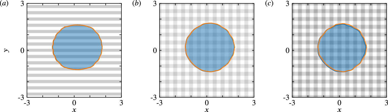
Approach A, trained on varied striped heterogeneity profiles given by equation (9). Comparison between FNO predictions (orange curves) and simulation data (blue curves and semi-transparent filled areas) at the end of the simulation interval, for profiles that are described by equation (9), but were not used in the training/testing dataset. The specific parameters used to describe the surface heterogeneities in each case are listed in Supplementary Appendix A. The surface profile is colored in shades of gray ranging between $ \Phi =2 $
(white) and
$ \Phi =2 $
(white) and $ \Phi =3 $
(black). For each case,
$ \Phi =3 $
(black). For each case, $ {E}_{\mathrm{aux}} $
is (a)
$ {E}_{\mathrm{aux}} $
is (a) $ 2.1 $
, (b)
$ 2.1 $
, (b) $ 1.5 $
, and (c)
$ 1.5 $
, and (c) $ 5.5\% $
, respectively.
$ 5.5\% $
, respectively.
3. Results
For all the tests presented herein, the generated datasets consist of snapshots of droplets that spread and travel over chemically heterogeneous surfaces, and in the absence of other body forces (e.g., gravity). The chosen value for the slip length is kept constant, namely $ \lambda ={10}^{-3} $
, the droplet volume is fixed at
$ \lambda ={10}^{-3} $
, the droplet volume is fixed at $ 2\pi $
and the initial contact line shape is the unit circle, whilst the profile of the chemical heterogeneity of the surface and the initial droplet position are allowed to vary across different samples in the datasets. The generated data used for training is converted to a polar representation that follows the centroid of the wetted area in terms of 128 uniformly distributed points on the contact line based on the azimuthal angle. Specific details on the datasets and heterogeneity profiles employed for each of the two approaches are provided in the following sections.
$ 2\pi $
and the initial contact line shape is the unit circle, whilst the profile of the chemical heterogeneity of the surface and the initial droplet position are allowed to vary across different samples in the datasets. The generated data used for training is converted to a polar representation that follows the centroid of the wetted area in terms of 128 uniformly distributed points on the contact line based on the azimuthal angle. Specific details on the datasets and heterogeneity profiles employed for each of the two approaches are provided in the following sections.
3.1. Approach A: The fully data-driven model
Significant preliminary effort has been invested in determining (i) the type of heterogeneity profiles $ \Phi \left(\boldsymbol{x}\right) $
that are necessary for a droplet to exhibit different types of behaviors for the model to learn (e.g., spreading, receding, excitation of higher harmonics, stick–slip dynamics, etc.), (ii) the time step
$ \Phi \left(\boldsymbol{x}\right) $
that are necessary for a droplet to exhibit different types of behaviors for the model to learn (e.g., spreading, receding, excitation of higher harmonics, stick–slip dynamics, etc.), (ii) the time step $ dt $
between the contact line snapshots at which the model is to be trained/queried, such that each snapshot varies sufficiently from one instance to the next, and (iii) the near-optimal model hyper-parameters that can provide reliable predictions on unseen samples, targeting a testing error,
$ dt $
between the contact line snapshots at which the model is to be trained/queried, such that each snapshot varies sufficiently from one instance to the next, and (iii) the near-optimal model hyper-parameters that can provide reliable predictions on unseen samples, targeting a testing error, $ {E}_{\mathrm{test}}^A $
, in the order of
$ {E}_{\mathrm{test}}^A $
, in the order of $ {10}^{-2} $
, see equation (4). For each of the training scenarios performed with approach A,
$ {10}^{-2} $
, see equation (4). For each of the training scenarios performed with approach A, $ {N}_{\mathrm{tot}} $
samples were generated, with 100 contact line snapshots per sample. Of these samples, 80% were used for training and the rest were used for testing. The models were trained using an initial learning rate of
$ {N}_{\mathrm{tot}} $
samples were generated, with 100 contact line snapshots per sample. Of these samples, 80% were used for training and the rest were used for testing. The models were trained using an initial learning rate of $ {10}^{-3} $
, which was then halved every 50 epochs. A rectified linear unit (ReLU) activation function was adopted, noting that other choices in preliminary runs resulted in less accurate models (see Supplementary Table 4). All other relevant AI parameters are mentioned in each of the following subsections.
$ {10}^{-3} $
, which was then halved every 50 epochs. A rectified linear unit (ReLU) activation function was adopted, noting that other choices in preliminary runs resulted in less accurate models (see Supplementary Table 4). All other relevant AI parameters are mentioned in each of the following subsections.
3.1.1. Training on varied striped profiles
The model is first trained with samples that combine horizontal and vertical striped features, assuming the form
 $$ \Phi \left(\boldsymbol{x}\right)=2+{p}_1\frac{1+\tanh \left({p}_2\cos \left({p}_3\pi x\right)\right)}{2}+{p}_4\frac{1+\tanh \left({p}_5\cos \left({p}_6\pi y\right)\right)}{2}, $$
where the parameters $ {p}_1,{p}_2,\dots, {p}_6 $
are uniformly distributed random numbers;
$ {p}_1,{p}_2,\dots, {p}_6 $
are uniformly distributed random numbers; $ {p}_1 $
and
$ {p}_1 $
and $ {p}_4 $
lie in the range
$ {p}_4 $
lie in the range $ \left[-\mathrm{0.5,0.5}\right] $
; the rest lie in the range
$ \left[-\mathrm{0.5,0.5}\right] $
; the rest lie in the range $ \left[-5,5\right] $
. With these parameter bounds, the local contact angle value range is
$ \left[-5,5\right] $
. With these parameter bounds, the local contact angle value range is $ 2<\Phi <3 $
. Therefore, each simulation run is unique, both in terms of the heterogeneity profile and the initial droplet position. The droplet motion was sampled until
$ 2<\Phi <3 $
. Therefore, each simulation run is unique, both in terms of the heterogeneity profile and the initial droplet position. The droplet motion was sampled until $ t=2 $
, such that in most cases the droplet was sufficiently close to its equilibrium position. The effect of the FNO-specific hyper-parameters is examined in Supplementary Appendix B, where it is shown that a hyperspace of 128 channels, with 2 Fourier layers retaining 8 Fourier modes, can be considered as the best model for this training (see Supplementary Table 1). The training and testing errors are shown in Figure 2 for different dataset sizes. The model with
$ t=2 $
, such that in most cases the droplet was sufficiently close to its equilibrium position. The effect of the FNO-specific hyper-parameters is examined in Supplementary Appendix B, where it is shown that a hyperspace of 128 channels, with 2 Fourier layers retaining 8 Fourier modes, can be considered as the best model for this training (see Supplementary Table 1). The training and testing errors are shown in Figure 2 for different dataset sizes. The model with $ {N}_{\mathrm{tot}}=600 $
manages to reach testing errors of about 0.4% and is used in subsequent model assessments.
$ {N}_{\mathrm{tot}}=600 $
manages to reach testing errors of about 0.4% and is used in subsequent model assessments.
Figure 3 compares the FNO predictions and the reference solutions at the end of the simulation for three different heterogeneity profiles, which were not included in the training dataset, but were constructed separately using equation (9) similar to the training samples (the specific parameter values are listed in Supplementary Appendix A). Visually inspecting the results with horizontal stripes (Figure 3a) and a combination of horizontal and vertical stripes (Figure 3b) suggests that the FNO predictions agree excellently with simulation results with $ {E}_{\mathrm{aux}} $
of approximately 2%. For both surfaces, the attainable values for
$ {E}_{\mathrm{aux}} $
of approximately 2%. For both surfaces, the attainable values for $ \Phi $
were in the range of
$ \Phi $
were in the range of $ 2<\Phi <2.5 $
. Upon broadening this range to
$ 2<\Phi <2.5 $
. Upon broadening this range to $ 2<\Phi <2.8 $
, increased
$ 2<\Phi <2.8 $
, increased $ {E}_{\mathrm{aux}} $
, but to a still acceptable value of about 5.5% (see Figure 3c). This degradation in the agreement may be attributed to the arguably limited number of samples used to capture a multi-dimensional parameter space (six surface parameters and two for the randomized initial droplet position), which appears to be also exacerbated by sharper and broader wettability contrasts.
$ {E}_{\mathrm{aux}} $
, but to a still acceptable value of about 5.5% (see Figure 3c). This degradation in the agreement may be attributed to the arguably limited number of samples used to capture a multi-dimensional parameter space (six surface parameters and two for the randomized initial droplet position), which appears to be also exacerbated by sharper and broader wettability contrasts.
For surface profiles that are not described by equation (9) and are therefore outside the training dataset distribution, the comparison of the FNO predictions against the reference solutions deteriorates. Figure 4 presents three such cases, referring the reader to Supplementary Appendix A for more details on the specific profiles for $ \Phi \left(\boldsymbol{x}\right) $
. Figure 4a shows a case which is similar to the training dataset but rotated by
$ \Phi \left(\boldsymbol{x}\right) $
. Figure 4a shows a case which is similar to the training dataset but rotated by $ {30}^{\circ } $
, Figure 4b shows a sample with smoothly varying random features and Figure 4c shows a sample with a large-scale wettability gradient, each attaining
$ {30}^{\circ } $
, Figure 4b shows a sample with smoothly varying random features and Figure 4c shows a sample with a large-scale wettability gradient, each attaining $ {E}_{\mathrm{aux}} $
values of 2.7, 11.4, and 56.9%, respectively. It is clear that, even though the model is well-trained and performs well on surfaces with heterogeneities that are drawn from the same distribution as the training dataset, it cannot generalize well enough outside this distribution. This is especially true for cases where the centroid of the droplet travels on the surface under the influence of pronounced wettability gradients, such as the test case shown in Figure 4c. A richer training dataset with increased complexity (in terms of heterogeneity profiles and therefore contact line shapes) should be considered to improve the model’s generalizability.
$ {E}_{\mathrm{aux}} $
values of 2.7, 11.4, and 56.9%, respectively. It is clear that, even though the model is well-trained and performs well on surfaces with heterogeneities that are drawn from the same distribution as the training dataset, it cannot generalize well enough outside this distribution. This is especially true for cases where the centroid of the droplet travels on the surface under the influence of pronounced wettability gradients, such as the test case shown in Figure 4c. A richer training dataset with increased complexity (in terms of heterogeneity profiles and therefore contact line shapes) should be considered to improve the model’s generalizability.
Approach A, trained on varied striped heterogeneity profiles given by equation (9). Comparison between FNO predictions (orange curves) and simulation data (blue curves and semi-transparent filled areas) at the end of the simulation interval, for profiles that cannot be described by equation (9) and are therefore outside the training distribution: (a) horizontal and vertical striped features, rotated by $ {30}^{\circ } $
, (b) smoothly varying random features, and (c) wettability gradient along the x-direction. The specific equations used to describe the surface heterogeneities in each case are given in Supplementary Appendix A. The substrate shading follows that of Figure 3. For each case, the auxiliary error is 2.7, 11.4, and 56.9%, respectively.
$ {30}^{\circ } $
, (b) smoothly varying random features, and (c) wettability gradient along the x-direction. The specific equations used to describe the surface heterogeneities in each case are given in Supplementary Appendix A. The substrate shading follows that of Figure 3. For each case, the auxiliary error is 2.7, 11.4, and 56.9%, respectively.

3.1.2. Training with more complex heterogeneity profiles
To improve upon the previous effort, a more complex heterogeneity profile is considered for generating the dataset, cast as a 7-parameter family of profiles of the form:
 $$ \Phi \left(\boldsymbol{x}\right)=1+{p}_1\tilde{x}+{p}_2\tanh \left[{p}_3\cos \left({p}_4\left(\tilde{x}\sin {p}_6+\tilde{y}\cos {p}_6\right)\right)\cos \left({p}_5\tilde{x}\right)\right], $$
where $ \tilde{x}=x\cos {p}_7-y\sin {p}_7 $
and
$ \tilde{x}=x\cos {p}_7-y\sin {p}_7 $
and $ \tilde{y}=x\sin {p}_7+y\cos {p}_7 $
. Parameters
$ \tilde{y}=x\sin {p}_7+y\cos {p}_7 $
. Parameters $ {p}_1,\dots, {p}_7 $
are uniformly distributed random numbers in the ranges
$ {p}_1,\dots, {p}_7 $
are uniformly distributed random numbers in the ranges $ {p}_1\in \left[0,1/15\right] $
,
$ {p}_1\in \left[0,1/15\right] $
, $ {p}_2\in \left[\mathrm{0,0.2}\right] $
,
$ {p}_2\in \left[\mathrm{0,0.2}\right] $
, $ {p}_3\in \left[-5,5\right] $
,
$ {p}_3\in \left[-5,5\right] $
, $ {p}_4,{p}_5\in \left[0,4\pi /3\right] $
,
$ {p}_4,{p}_5\in \left[0,4\pi /3\right] $
, $ {p}_6\in \left[-\pi /2,+\pi /2\right] $
, and
$ {p}_6\in \left[-\pi /2,+\pi /2\right] $
, and $ {p}_7\in \left[-\pi, +\pi \right] $
.
$ {p}_7\in \left[-\pi, +\pi \right] $
.
Qualitatively, profiles of this form include heterogeneities that superimpose a wettability gradient and secondary features in terms of angled checkerboard patterns, which may also degenerate to striped patterns (see, e.g., Figure 6 for some representative profiles generated by equation (10). More specifically, $ {p}_1 $
controls the strength of the gradient, whereas
$ {p}_1 $
controls the strength of the gradient, whereas $ {p}_2 $
and
$ {p}_2 $
and $ {p}_3 $
control the wettability contrast and the steepness of the secondary features, respectively. Parameters
$ {p}_3 $
control the wettability contrast and the steepness of the secondary features, respectively. Parameters $ {p}_4 $
and
$ {p}_4 $
and $ {p}_5 $
set the wavelength of the secondary features, whereas
$ {p}_5 $
set the wavelength of the secondary features, whereas $ {p}_6 $
and
$ {p}_6 $
and $ {p}_7 $
represent random rotations of secondary features and the gradient, respectively. In collecting the data necessary for the training and testing, care was taken to ensure that all simulations corresponding to each realization of equation (10) and its initial conditions resulted in dynamics that conformed with the requirement
$ {p}_7 $
represent random rotations of secondary features and the gradient, respectively. In collecting the data necessary for the training and testing, care was taken to ensure that all simulations corresponding to each realization of equation (10) and its initial conditions resulted in dynamics that conformed with the requirement $ \Phi \left(\boldsymbol{c}(t)\right)>0 $
for all
$ \Phi \left(\boldsymbol{c}(t)\right)>0 $
for all $ t>0 $
.
$ t>0 $
.
For each sample heterogeneity profile, a simulation run of 400 dimensionless time units is performed to allow for sufficient time for a droplet to move in the presence of wettability gradients, within which 100 contact line snapshots are uniformly sampled. Supplementary Appendix B presents the parametric exploration of the FNO-specific hyper-parameters, motivating the choice of a hyperspace with 128 channels and 2 Fourier layers retaining 8 Fourier modes, as the best choice for this effort (see Supplementary Table 2). Figure 5 shows the training and testing errors for different dataset sizes, revealing that the model with $ {N}_{\mathrm{tot}}=2000 $
achieves testing errors as low as 0.4% and is used to produce the results in this section. The increased dataset size compensates for the increased complexity of the surface heterogeneities considered, leading to a testing error which is of the same order as in Section 3.1.1.
$ {N}_{\mathrm{tot}}=2000 $
achieves testing errors as low as 0.4% and is used to produce the results in this section. The increased dataset size compensates for the increased complexity of the surface heterogeneities considered, leading to a testing error which is of the same order as in Section 3.1.1.
Approach A, trained on heterogeneity profiles given by equation (10). Training and testing errors as a function of the number of epochs for three different datasets with $ {N}_{\mathrm{tot}} $
= 500 (red curves;
$ {N}_{\mathrm{tot}} $
= 500 (red curves; $ {N}_{\mathrm{train}} $
= 400 and
$ {N}_{\mathrm{train}} $
= 400 and $ {N}_{\mathrm{test}} $
= 100),
$ {N}_{\mathrm{test}} $
= 100), $ {N}_{\mathrm{tot}} $
= 1000 (blue curves;
$ {N}_{\mathrm{tot}} $
= 1000 (blue curves; $ {N}_{\mathrm{train}} $
= 800 and
$ {N}_{\mathrm{train}} $
= 800 and $ {N}_{\mathrm{test}} $
= 200), and
$ {N}_{\mathrm{test}} $
= 200), and $ {N}_{\mathrm{tot}} $
= 2000 (black curves;
$ {N}_{\mathrm{tot}} $
= 2000 (black curves; $ {N}_{\mathrm{train}} $
= 1600 and
$ {N}_{\mathrm{train}} $
= 1600 and $ {N}_{\mathrm{test}} $
= 400). Dashed and solid curves show the training errors
$ {N}_{\mathrm{test}} $
= 400). Dashed and solid curves show the training errors $ {E}_{\mathrm{train}}^{\mathrm{A}} $
and testing errors
$ {E}_{\mathrm{train}}^{\mathrm{A}} $
and testing errors $ {E}_{\mathrm{test}}^{\mathrm{A}} $
, respectively.
$ {E}_{\mathrm{test}}^{\mathrm{A}} $
, respectively.

Figure 6 compares the FNO predictions and the reference solution for six cases that can be expressed by equation (10), albeit not used during the AI training (specific parameters used to describe the heterogeneities for each case are listed in Supplementary Appendix A). Even though the model performance is generally less favorable than the one presented in the previous section, it is able to capture a greater variety of behaviors. In the cases where the droplet primarily spreads on the heterogeneous surface without moving appreciably from its initial position (e.g., Figure 6a,c), the model performs moderately well, with $ {E}_{\mathrm{aux}}\lesssim 10\% $
. In other scenarios, where the droplet is traveling on the surface and the heterogeneities are more complex, the model performance deteriorates, with much larger discrepancies between the predicted contact line position and the reference solution. Also noteworthy is that the predicted contact lines develop unphysical instabilities, most notably observed in Figure 6b,e, where the variations in the surface features are relatively smooth and do not justify the contact line protrusions predicted by the model.
$ {E}_{\mathrm{aux}}\lesssim 10\% $
. In other scenarios, where the droplet is traveling on the surface and the heterogeneities are more complex, the model performance deteriorates, with much larger discrepancies between the predicted contact line position and the reference solution. Also noteworthy is that the predicted contact lines develop unphysical instabilities, most notably observed in Figure 6b,e, where the variations in the surface features are relatively smooth and do not justify the contact line protrusions predicted by the model.
Approach A, trained on heterogeneity profiles given by equation (10), comparing the FNO predictions (orange curves) and simulation data (blue curves and semi-transparent filled areas) at the beginning (circular contact lines) and the end of the simulation interval for different realizations of equation (10) that were not used during training/testing. The specific parameters used to describe the heterogeneities in each case are given in Supplementary Appendix A. The surface profile is colored in shades of gray ranging between $ \Phi =1 $
(white) and
$ \Phi =1 $
(white) and $ \Phi =2 $
(black). The value of the auxiliary error for each case is (a) 10.2%, (b) 13.1%, (c) 5.1%, (d) 31.4%, (e) 77.2%, and (f) 49.3%.
$ \Phi =2 $
(black). The value of the auxiliary error for each case is (a) 10.2%, (b) 13.1%, (c) 5.1%, (d) 31.4%, (e) 77.2%, and (f) 49.3%.

3.1.3. Overall assessment
At this stage, we have gathered sufficient evidence to offer some commentary in relation to the performance of Approach A, which, as mentioned previously, is similar in spirit as the approach followed in the original contribution by Li et al. (Reference Li, Kovachki, Azizzadenesheli, Liu, Bhattacharya, Stuart and Anandkumar2020) who proposed the FNO architecture. Specifically, we have identified the following shortcomings that potentially severely limit the applicability of such models in the context of wetting:
Limited generalizability. This approach works generally well only if the unseen surface heterogeneity profiles are relatively simple (e.g., no significant movement of the droplet centroid) and are drawn from the same distribution as the heterogeneity profiles in the training dataset. Unlike the test cases considered in the original contribution of Li et al. (Reference Li, Kovachki, Azizzadenesheli, Liu, Bhattacharya, Stuart and Anandkumar2020), the parameter space herein considered is inherently multi-dimensional. This is rather limiting, because there can exist countless parameters that can be used to describe heterogeneity features, such as their arrangement, smoothness, the wettability contrast, and so forth. This has an adverse effect on the requirements for the size of the training dataset, which needs to be sufficiently large to accommodate a broad representation of the effects of the different heterogeneity characteristics that a surface may possess. Hence, this approach has significant generalization challenges that may only be overcome by supplementing the training dataset with types of heterogeneity profiles that are qualitatively similar to the target testing scenarios.
Solution can only be queried at fixed intervals; using the data-driven model requires part of the simulation to be completed. A number of sequential solutions is required to provide a reliable estimation of the subsequent solution, the temporal spacing of which is problem-dependent and therefore limits the generalizability of this approach even further. Moreover, these solutions should be uniformly spaced in time while the subsequent solution can only be predicted at a fixed step, respecting the uniform time spacing of the previous solutions. In the case presented here, 10 initial solutions were deemed adequate to provide a reasonable prediction for the next 90 solutions. In the case of longer simulations with a larger number of solutions to be predicted, it is possible that more solutions should be used as input to the model. Therefore, this approach requires simulating the initial stages of the target testing scenario (in the present study this amounts to 10% of the simulation), before deploying the data-driven model for predicting how the contact line evolves.
3.2. Approach B: AI-augmented model for the contact line velocity
In an effort to move past the limitations listed above, approach B, presented in Section 2.2.2, is followed here, using the same dataset as in Section 3.1.2 to facilitate a fair comparison between the two approaches. Thus, instead of using information for the heterogeneity profiles which was necessary for approach A, approach B includes the leading-order term of the contact line velocity $ {\overline{v}}_{\nu } $
in the input data. The rest of the details of the training process remain the same, apart from the FNO-related hyper-parameters, an exploration of which is presented in Supplementary Appendix B. Specifically, in Supplementary Table 3, we see that the architecture with 128 channels with 4 Fourier layers retaining 16 Fourier modes gives the best performance in the explored parameter range. In addition, a Gaussian error linear unit (GELU) was used as the activation function since it was found to provide the most accurate results (see Supplementary Table 4).
$ {\overline{v}}_{\nu } $
in the input data. The rest of the details of the training process remain the same, apart from the FNO-related hyper-parameters, an exploration of which is presented in Supplementary Appendix B. Specifically, in Supplementary Table 3, we see that the architecture with 128 channels with 4 Fourier layers retaining 16 Fourier modes gives the best performance in the explored parameter range. In addition, a Gaussian error linear unit (GELU) was used as the activation function since it was found to provide the most accurate results (see Supplementary Table 4).
Figure 7 presents the training and testing errors, defined in equation (7), as a function of the number of epochs, for different dataset sizes. An initial learning rate of $ {10}^{-3} $
is used, which was halved every 50 epochs. Within this approach, the model with
$ {10}^{-3} $
is used, which was halved every 50 epochs. Within this approach, the model with $ {N}_{\mathrm{tot}}=2000 $
achieves testing errors of 10% and is used for the results presented in this section. It is worth noting that, even though this error is significantly larger compared to the one obtained in Section 3.1.2, the presence of the leading-order term already provides a reasonable initial estimate for the contact line velocity. It is the correction to this estimate that the data-driven model under approach B tries to capture, which, in some cases, is close to zero thus producing large relative errors as it appears in the denominator of the summand in equation (7).
$ {N}_{\mathrm{tot}}=2000 $
achieves testing errors of 10% and is used for the results presented in this section. It is worth noting that, even though this error is significantly larger compared to the one obtained in Section 3.1.2, the presence of the leading-order term already provides a reasonable initial estimate for the contact line velocity. It is the correction to this estimate that the data-driven model under approach B tries to capture, which, in some cases, is close to zero thus producing large relative errors as it appears in the denominator of the summand in equation (7).
Approach B, trained on heterogeneity profiles given by equation (10). Training and testing errors as a function of the number of epochs for three different datasets with $ {N}_{\mathrm{tot}} $
= 500 (red curves;
$ {N}_{\mathrm{tot}} $
= 500 (red curves; $ {N}_{\mathrm{train}} $
= 400 and
$ {N}_{\mathrm{train}} $
= 400 and $ {N}_{\mathrm{test}} $
= 100),
$ {N}_{\mathrm{test}} $
= 100), $ {N}_{\mathrm{tot}} $
= 1000 (blue curves;
$ {N}_{\mathrm{tot}} $
= 1000 (blue curves; $ {N}_{\mathrm{train}} $
= 800 and
$ {N}_{\mathrm{train}} $
= 800 and $ {N}_{\mathrm{test}} $
= 200), and
$ {N}_{\mathrm{test}} $
= 200), and $ {N}_{\mathrm{tot}} $
= 2000 (black curves;
$ {N}_{\mathrm{tot}} $
= 2000 (black curves; $ {N}_{\mathrm{train}} $
= 1600 and
$ {N}_{\mathrm{train}} $
= 1600 and $ {N}_{\mathrm{test}} $
= 400). Dashed and solid curves show the training errors
$ {N}_{\mathrm{test}} $
= 400). Dashed and solid curves show the training errors $ {E}_{\mathrm{train}}^{\mathrm{A}} $
and testing errors
$ {E}_{\mathrm{train}}^{\mathrm{A}} $
and testing errors $ {E}_{\mathrm{test}}^{\mathrm{A}} $
, respectively.
$ {E}_{\mathrm{test}}^{\mathrm{A}} $
, respectively.

After developing a data-driven counterpart to $ \mathcal{H} $
in equation (5), we advance the solution in time with a time-stepping routine. Specifically, we employ a third-order explicit Runge–Kutta method (Bogacki and Shampine, Reference Bogacki and Shampine1989) within the scipy.integrate.solve_ivp solver in Python, noting that this choice is a good compromise between accuracy and efficiency as it requires only a few forward passes through the AI model per time step. Nonetheless, this specific time-stepping scheme is not in any way a prerequisite of this approach, as other time integration schemes can be applied with similarly accurate results. Figure 8 compares the AI-augmented predictions based on approach B against the reference simulation results, for the same cases shown in Figure 6. As evidenced, the agreement is much improved compared to approach A, exhibiting low values for
$ \mathcal{H} $
in equation (5), we advance the solution in time with a time-stepping routine. Specifically, we employ a third-order explicit Runge–Kutta method (Bogacki and Shampine, Reference Bogacki and Shampine1989) within the scipy.integrate.solve_ivp solver in Python, noting that this choice is a good compromise between accuracy and efficiency as it requires only a few forward passes through the AI model per time step. Nonetheless, this specific time-stepping scheme is not in any way a prerequisite of this approach, as other time integration schemes can be applied with similarly accurate results. Figure 8 compares the AI-augmented predictions based on approach B against the reference simulation results, for the same cases shown in Figure 6. As evidenced, the agreement is much improved compared to approach A, exhibiting low values for $ {E}_{\mathrm{aux}} $
without the nonphysical contact line protrusions that were observed previously.
$ {E}_{\mathrm{aux}} $
without the nonphysical contact line protrusions that were observed previously.
Approach B, trained on heterogeneity profiles given by equation (10), comparing the FNO predictions (orange curves), and the reference simulation solutions (blue curves and semi-transparent filled areas) using the same heterogeneity profiles of Figure 6. The value of the auxiliary error for each case is (a) 2.3%, (b) 4.5%, (c) 1.1%, (d) 2.6%, (e) 0.9%, and (f) 8.1%, much lower compared to the values reported, in Figure 6.

To assess the generalization capabilities of this approach, Figure 9 shows comparisons for heterogeneity profiles that are described by equation (10), but the specific values for the equation parameters are well outside their corresponding ranges considered during training. More specifically, the heterogeneity profiles used are variations of the profile of Figure 8d. In Figure 9a, a value of $ {p}_3=10 $
is used, leading to significantly sharper checkerboard patterns compared to those obtained with
$ {p}_3=10 $
is used, leading to significantly sharper checkerboard patterns compared to those obtained with $ {p}_3\in \left[-5,5\right] $
for the training dataset. The model performs in a very satisfactory manner with an auxiliary error of 4.0%, which is slightly elevated compared to the error obtained in the original case, see Figure 8d. Of course, as the sharpness of these features increases further, numerical instabilities may occur if the number of harmonics considered is not sufficiently large to capture the high-frequency components in the contact line profile. This already makes the simulation problem challenging itself, and this would possibly be a regime where the AI-driven model may also struggle to accurately resolve. In Figure 9b, a value of
$ {p}_3\in \left[-5,5\right] $
for the training dataset. The model performs in a very satisfactory manner with an auxiliary error of 4.0%, which is slightly elevated compared to the error obtained in the original case, see Figure 8d. Of course, as the sharpness of these features increases further, numerical instabilities may occur if the number of harmonics considered is not sufficiently large to capture the high-frequency components in the contact line profile. This already makes the simulation problem challenging itself, and this would possibly be a regime where the AI-driven model may also struggle to accurately resolve. In Figure 9b, a value of $ {p}_2=0.4 $
is used, resulting in a higher wettability contrast in the checkerboard pattern compared to those seen during training with
$ {p}_2=0.4 $
is used, resulting in a higher wettability contrast in the checkerboard pattern compared to those seen during training with $ {p}_2\in \left[\mathrm{0,0.2}\right] $
. In this case, the droplet is only able to spread as it cannot overcome the wettability barrier, with an auxiliary error of only 3.0%. A third example, see Figure 9c, presents a case where
$ {p}_2\in \left[\mathrm{0,0.2}\right] $
. In this case, the droplet is only able to spread as it cannot overcome the wettability barrier, with an auxiliary error of only 3.0%. A third example, see Figure 9c, presents a case where $ {p}_2=0.4 $
and
$ {p}_2=0.4 $
and $ {p}_1=0.1 $
, imposing a steeper background gradient compared to the range of values considered for
$ {p}_1=0.1 $
, imposing a steeper background gradient compared to the range of values considered for $ {p}_1 $
during training. In this case, the droplet moves further along the wetabillity gradient, exhibiting an auxiliary error of 11.7%. A closer inspection reveals that this disagreement stems from the more pronounced stick–slip events that occur, whereby the depinning of the contact line is more likely to be mistimed compared to the reference solution. This observation was also made in the context of asymptotic models for contact line dynamics (Savva and Kalliadasis, Reference Savva and Kalliadasis2011). Nonetheless, the agreement between the two solutions is very satisfactory, leading us to conclude that the AI-assisted approach presented here is able to handle more challenging heterogeneity profiles compared to the ones encountered during training.
$ {p}_1 $
during training. In this case, the droplet moves further along the wetabillity gradient, exhibiting an auxiliary error of 11.7%. A closer inspection reveals that this disagreement stems from the more pronounced stick–slip events that occur, whereby the depinning of the contact line is more likely to be mistimed compared to the reference solution. This observation was also made in the context of asymptotic models for contact line dynamics (Savva and Kalliadasis, Reference Savva and Kalliadasis2011). Nonetheless, the agreement between the two solutions is very satisfactory, leading us to conclude that the AI-assisted approach presented here is able to handle more challenging heterogeneity profiles compared to the ones encountered during training.
Exploring the range of applicability of approach B. The plots compare the FNO predictions in accordance with equation (5) (orange curves) and the reference solutions (blue curves and semi-transparent filled areas) for the contact line positions at the start and the end of simulations, as the droplet traverses the features of the surface. All heterogeneity profiles are derived from the profile used in Figure 8d (see equation (10) with the actual parameters given in Supplementary Appendix A) by altering the value of a single parameter in each case: (a) $ {p}_3=10 $
; (b)
$ {p}_3=10 $
; (b) $ {p}_2=0.4 $
; (c)
$ {p}_2=0.4 $
; (c) $ {p}_1=0.1 $
and
$ {p}_1=0.1 $
and $ {p}_2=0.4 $
. The heterogeneity profiles are colored in shades of gray, ranging between
$ {p}_2=0.4 $
. The heterogeneity profiles are colored in shades of gray, ranging between $ \Phi =1 $
(white) and
$ \Phi =1 $
(white) and $ \Phi =2 $
(black).
$ \Phi =2 $
(black).

Figure 10 further demonstrates the generalization capabilities of the model trained with the second approach in significantly different heterogeneity profiles. Figure 10a shows the movement of a droplet on a heterogeneous surface featuring the superposition of a checkerboard pattern and a gradient that turns around a wettability barrier (see Supplementary Appendix A for the specific equation for $ \Phi \left(\boldsymbol{x}\right) $
). In this setup, the droplet starts from the upper left region and undergoes a long excursion away from its initial position to settle on the more hydrophilic part of the surface on the lower left region. Such a surface profile is considerably more complex than the family of profiles the AI-augmented model was trained on, see equation (10). Moreover, as shown in this figure, a simulation with the leading-order term alone,
$ \Phi \left(\boldsymbol{x}\right) $
). In this setup, the droplet starts from the upper left region and undergoes a long excursion away from its initial position to settle on the more hydrophilic part of the surface on the lower left region. Such a surface profile is considerably more complex than the family of profiles the AI-augmented model was trained on, see equation (10). Moreover, as shown in this figure, a simulation with the leading-order term alone, $ {\upsilon}_{\nu }={\overline{\upsilon}}_{\nu } $
, leads to large discrepancies throughout the simulation. Upon augmenting the low-order model with its AI correction, the errors considerably diminish, with
$ {\upsilon}_{\nu }={\overline{\upsilon}}_{\nu } $
, leads to large discrepancies throughout the simulation. Upon augmenting the low-order model with its AI correction, the errors considerably diminish, with $ {E}_{\mathrm{aux}} $
at about 1.6% on the final solution. This further supports the idea that the leading term already captures the effect of the heterogeneity features, allowing approach B to better capture the dynamics on unseen
$ {E}_{\mathrm{aux}} $
at about 1.6% on the final solution. This further supports the idea that the leading term already captures the effect of the heterogeneity features, allowing approach B to better capture the dynamics on unseen $ \Phi \left(\boldsymbol{x}\right) $
, whilst requiring fewer data. A second example is provided in Figure 10b in which a broader contact angle range is used than the one used during training, and the slip length is changed to
$ \Phi \left(\boldsymbol{x}\right) $
, whilst requiring fewer data. A second example is provided in Figure 10b in which a broader contact angle range is used than the one used during training, and the slip length is changed to $ \lambda ={10}^{-5} $
, two orders of magnitude smaller than the value used to generate the training dataset,
$ \lambda ={10}^{-5} $
, two orders of magnitude smaller than the value used to generate the training dataset, $ \lambda ={10}^{-3} $
. Despite these appreciable changes, the AI predictions are in a good agreement with the reference simulation results, with
$ \lambda ={10}^{-3} $
. Despite these appreciable changes, the AI predictions are in a good agreement with the reference simulation results, with $ {E}_{\mathrm{aux}} $
at about 4.0% at the end of the simulation. As in Figure 10a, the predictions of the leading-order term are visibly inaccurate, but the AI model is able to correct these predictions successfully. These observations highlight the capacity of the AI-augmented model to generalize beyond the cases encountered during the training phase as long as the training samples exhibit sufficiently rich behaviors.
$ {E}_{\mathrm{aux}} $
at about 4.0% at the end of the simulation. As in Figure 10a, the predictions of the leading-order term are visibly inaccurate, but the AI model is able to correct these predictions successfully. These observations highlight the capacity of the AI-augmented model to generalize beyond the cases encountered during the training phase as long as the training samples exhibit sufficiently rich behaviors.
Generalizability of approach B. The plots compare the FNO predictions in accordance with equation (5) (orange curves), simulation results of the model that takes $ {v}_{\nu }={\overline{v}}_{\nu } $
defined in equation (5) (green curves), and the reference solutions (blue curves and semi-transparent filled areas) for the contact line positions in several time instances as the droplet traverses the features of the surface for (a) a surface profile that is markedly different from the heterogeneity profiles used in training/testing, and (b) a profile that covers a broader range of contact angles and for
$ {v}_{\nu }={\overline{v}}_{\nu } $
defined in equation (5) (green curves), and the reference solutions (blue curves and semi-transparent filled areas) for the contact line positions in several time instances as the droplet traverses the features of the surface for (a) a surface profile that is markedly different from the heterogeneity profiles used in training/testing, and (b) a profile that covers a broader range of contact angles and for $ \lambda ={10}^{-5} $
, two orders of magnitude smaller than the value used for training. The specific equations used to describe the heterogeneities in each case are given in Supplementary Appendix A. The surface profiles are colored in shades of gray, ranging between (a)
$ \lambda ={10}^{-5} $
, two orders of magnitude smaller than the value used for training. The specific equations used to describe the heterogeneities in each case are given in Supplementary Appendix A. The surface profiles are colored in shades of gray, ranging between (a) $ \Phi =1 $
(white) and
$ \Phi =1 $
(white) and $ \Phi =2 $
(black), and (b)
$ \Phi =2 $
(black), and (b) $ \Phi =1 $
(white) and
$ \Phi =1 $
(white) and $ \Phi =3 $
(black).
$ \Phi =3 $
(black).

The improved performance documented in this section demonstrates that approach B overcomes the main drawbacks of approach A, presented at the end of Section 3.1. The only drawback of approach B is the reliance on standard time integration schemes to advance the solution in time. This requirement entails a longer testing time, especially in case adaptive time stepping is used to meet the stability criteria of the scheme, thus also increasing the number of times the network needs to be evaluated. However, this feature is not too restrictive, because both the forward pass in the FNO model and the calculations of the leading-order term are comparatively much cheaper than solving the governing model given by equations (1a)–(1d). Although approach A is able to almost instantaneously predict the contact line evolution, it is to be noted that in order to be able to start using the FNO network, a considerable portion of the simulation needs to be completed by a standard solver, thus making the overall computational cost much greater compared to the cost required for a simulation based on approach B.
4. Conclusions
This study explored two data-driven approaches for modeling the motion of droplets on chemically heterogeneous surfaces, which are based on the FNO. The first approach follows a fully data-driven pathway, where, the neural network is used in an iterative manner for predicting the solution at fixed time intervals, whereas the second augments a leading-order analytical model for the contact line velocity with a data-driven component, which is then used to advance the solution with standard time integration schemes. The second approach possesses a significant performance advantage in terms of model accuracy and generalizability. The key feature behind the success of the second approach is the fact that the model already encodes some of the physics and the AI model is tasked to learn corrections to that model. In addition, this approach retains the capabilities of the FNO to be used on different grids, without the need to retrain the model.
We should emphasize that, for the system considered here, an asymptotic model is readily available and it can already efficiently and accurately resolve the motion of droplets on chemically heterogeneous surfaces (Savva et al., Reference Savva, Groves and Kalliadasis2019). However, the work undertaken here constitutes a proof-of-concept study that may be extended, generalized, and refined for other situations where such asymptotic models are not available. For example, the inclusion of further complexities (e.g., body forces) quickly renders asymptotic analyses intractable, whereas resorting to this type of data-driven surrogate modeling approach appears to be a viable alternative to expensive direct numerical simulations.
The present work also opens a number of possibilities for further exploration in forthcoming studies. First, the findings of this study can guide the generation of the corresponding direct numerical simulation datasets for deploying this data-driven workflow on high-fidelity simulations that go beyond the long-wave limit, considering improvements upon simple models that are applicable for larger contact angles (Cox, Reference Cox1986; Snoeijer, Reference Snoeijer2006; Afkhami et al., Reference Afkhami, Buongiorno, Guion, Popinet, Saade, Scardovelli and Zaleski2018). In addition, such efficient surrogates may be leveraged in informing strategies for controllable droplet transport, by accelerating the use of inverse modeling approaches for the design of surface features, alleviating long design cycles that typically rely on trial and error through experiments and/or computationally demanding multi-dimensional parametric studies through direct numerical simulations.
Acknowledgments
We are grateful for the support of the Centre of Excellence (CoE) Research on AI and Simulation-Based Engineering at Exascale (RAISE, https://www.coe-raise.eu/), in the form of training workshops, technical meetings, and administration support.
Author contribution
Conceptualization: N.S.; Data curation: A.D.D.; Formal analysis: N.S., A.D.D.; Funding acquisition: N.S.; Investigation: N.S., A.D.D.; Methodology: N.S., A.D.D.; Resources: N.S.; Software: N.S., A.D.D.; Validation: N.S., A.D.D.; Visualization: N.S., A.D.D.; Writing—original draft: A.D.D.; Writing—review and editing: N.S. All authors approved the final submitted draft.
Competing interest
The authors declare none.
Data availability statement
The codes and datasets used for the training and testing, along with the trained AI models are freely available at https://www.coe-raise.eu/od-wl.
Funding statement
The research leading to these results has been conducted in the CoE RAISE project, which receives funding from the European Union’s Horizon 2020—Research and Innovation Framework Programme H2020-INFRAEDI-2019-1 under Grant Agreement No. 951733. We also acknowledge support by project SimEA, funded by the European Union’s Horizon 2020 Research and Innovation Programme under Grant Agreement No. 810660. Furthermore, this work was supported by computing time awarded on the Cyclone supercomputer of the High Performance Computing Facility of The Cyprus Institute, under project ID PRO21B104.
Ethical standard
The research meets all ethical guidelines, including adherence to the legal requirements of the study country.
Supplementary material
The supplementary material for this article can be found at http://doi.org/10.1017/dce.2023.19.


 Open access
Comments
No Comments have been published for this article.