










1 Introduction
For any function f on the complex unit disk ${\mathbb {D}}$
, let
${\mathbb {D}}$
, let
 . In his 1952 PhD thesis, H. S. Shapiro [Reference Shapiro19, § 2.8] studied the following problem (cf. also his Master’s thesis [Reference Shapiro18] with the same title):
Problem 1.1 (Shapiro, 1952)
For integers $d>n\geq 0$
, determine the maximum
$d>n\geq 0$
, determine the maximum $\mathscr {M}_{n,d}$
of
$\mathscr {M}_{n,d}$
of
 $$ \begin{align} \left\lvert { a_0+a_1+\ldots+a_n } \right\rvert , \end{align} $$
over all polynomials $f = a_0 + a_1 X + \ldots + a_{d-1} X^{d-1} \in {\mathbb {C}}[X]$
of degree strictly less than d with
$f = a_0 + a_1 X + \ldots + a_{d-1} X^{d-1} \in {\mathbb {C}}[X]$
of degree strictly less than d with $ \left \lVert {f} \right \rVert _\infty \leq 1$
.
$ \left \lVert {f} \right \rVert _\infty \leq 1$
.
Clearly, Problem 1.1 may be viewed as determining the operator norm of a certain linear functional (here the underlying space being ${\mathbb {C}}[X]^{<d}$
, the space of polynomials of degree
${\mathbb {C}}[X]^{<d}$
, the space of polynomials of degree $<d$
). This relates the present problem to a vast family of problems in functional analysis and adjacent fields, the scope of which we cannot possibly frame here in a just manner.
$<d$
). This relates the present problem to a vast family of problems in functional analysis and adjacent fields, the scope of which we cannot possibly frame here in a just manner.
More concretely, the motivation for Shapiro’s question seems to have been (at least in part) a result of Landau, who had determined the maximum of (1.1) when instead f ranges over all 1-bounded holomorphic functions on the unit disk (see [Reference Landau8] or [Reference Landau9, pp. 20–23]):
Theorem 1.2 (Landau, 1913)
Let n be a non-negative integer. Then, for any holomorphic function f on ${\mathbb {D}}$
with
${\mathbb {D}}$
with $ \left \lVert {f} \right \rVert _\infty \leq 1$
and power series expansion
$ \left \lVert {f} \right \rVert _\infty \leq 1$
and power series expansion $f(z) = a_0 + a_1 z + a_2 z^2 + \ldots $
, one has
$f(z) = a_0 + a_1 z + a_2 z^2 + \ldots $
, one has

where
 $$ \begin{align} \binom{-1/2}{\nu} = \prod_{\kappa=0}^{\nu-1} \frac{-1/2-\kappa}{\nu-\kappa} = (-1)^\nu \frac{1\cdot 3\cdot \ldots \cdot (2\nu-1)}{2\cdot 4\cdot \ldots \cdot 2\nu}. \end{align} $$
Moreover, ‘ $\leq $
’ in (1.2) is attained with equality precisely for the rational function
$\leq $
’ in (1.2) is attained with equality precisely for the rational function $f_n$
given by
$f_n$
given by
 $$ \begin{align} f_n(z) = \frac{z^n P_n(1/z)}{P_n(z)}, \quad\text{where}\quad P_n(z) = \sum_{\nu=0}^n \binom{-1/2}{\nu} (-z)^\nu, \end{align} $$
and the functions $\eta f_n$
, where
$\eta f_n$
, where $\eta $
is any unimodular constant.
$\eta $
is any unimodular constant.
Remark. Landau [Reference Landau8, Reference Landau9] proves the asymptotic in (1.2) with an error term $o(\log n)$
rather than
$o(\log n)$
rather than $O(1)$
. The proof is based on Stirling’s formula. Newman [Reference Newman11] cites Landau’s result with the stronger error term
$O(1)$
. The proof is based on Stirling’s formula. Newman [Reference Newman11] cites Landau’s result with the stronger error term $O(1)$
. Regardless, the latter version is immediate from Landau’s proof upon using a stronger form of Stirling’s formula.
$O(1)$
. Regardless, the latter version is immediate from Landau’s proof upon using a stronger form of Stirling’s formula.
Let us now restrict attention to those f in Theorem 1.2 which are polynomials of degree $<d$
. By compactness, the set of all possible numbers produced by the left hand side of (1.2) admits a maximum
$<d$
. By compactness, the set of all possible numbers produced by the left hand side of (1.2) admits a maximum $\mathscr {M}_{n,d}$
(recall Problem 1.1). As the extremal function
$\mathscr {M}_{n,d}$
(recall Problem 1.1). As the extremal function $f_n$
in Theorem 1.2 is only a polynomial for
$f_n$
in Theorem 1.2 is only a polynomial for $n=0$
, we have the strict inequality
$n=0$
, we have the strict inequality
 $$ \begin{align} \mathscr{M}_{n,d} < \mathscr{L}_n \quad (\leq \mathscr{L}_d). \end{align} $$
(For a reasonably self-contained justification of this inequality, see Proposition 4.1 below.) Despite this, in a stroke of genius, Newman [Reference Newman11] was able to compute the numbers $\mathscr {M}_{n-1,2n}$
exactly:
$\mathscr {M}_{n-1,2n}$
exactly:
Theorem 1.3 (Newman, 1978)
Let n be a non-negative integer. Then, for every polynomial $f = \sum _\nu a_\nu X^\nu \in {\mathbb {C}}[X]^{<2n}$
with
$f = \sum _\nu a_\nu X^\nu \in {\mathbb {C}}[X]^{<2n}$
with $ \left \lVert {f} \right \rVert _\infty \leq 1$
, one has
$ \left \lVert {f} \right \rVert _\infty \leq 1$
, one has
 $$ \begin{align} \left\lvert { a_0+a_1+\ldots+a_{n-1} } \right\rvert \leq \frac{1}{2} + \frac{1}{n} \sum_{\omega^n = -1} \frac{1}{ \left\lvert {\omega-1} \right\rvert }. \end{align} $$
(Here the sum ranges over all complex numbers $\omega $
with
$\omega $
with $\omega ^n=-1$
.) Moreover, ‘
$\omega ^n=-1$
.) Moreover, ‘ $\leq $
’ in (1.6) is attained with equality for some polynomial satisfying the above conditions; in other words,
$\leq $
’ in (1.6) is attained with equality for some polynomial satisfying the above conditions; in other words,
 $$ \begin{align} \mathscr{M}_{n-1,2n} = \frac{1}{2} + \frac{1}{n} \sum_{\omega^n = -1} \frac{1}{ \lvert {\omega-1} \rvert } \quad \left( { = \frac{\log n}{\pi}+O(1) } \right). \end{align} $$
We conclude this section with a short remark on the real case, i.e., inequalities for coefficient sums of real polynomials that are bounded by $1$
on the interval
$1$
on the interval $[-1,1]$
. In 1892, Markov established sharp bounds for the derivatives of such polynomials (see [Reference Markov10, p. 258]). The question analogous to (1.1) seems to have first been considered by Reimer and Zeller [Reference Reimer and Zeller14] who established sharp bounds for even/odd polynomials (see also [Reference Rack13] and the references therein). As in the above complex setting, the current state of knowledge concerning the real case seems to be similarly fragmented and leaves much to be desired. Regardless, the methods that have been used to study the real situation have a somewhat different flavour, and in the present investigation we shall restrict our attention to the complex case.
$[-1,1]$
. In 1892, Markov established sharp bounds for the derivatives of such polynomials (see [Reference Markov10, p. 258]). The question analogous to (1.1) seems to have first been considered by Reimer and Zeller [Reference Reimer and Zeller14] who established sharp bounds for even/odd polynomials (see also [Reference Rack13] and the references therein). As in the above complex setting, the current state of knowledge concerning the real case seems to be similarly fragmented and leaves much to be desired. Regardless, the methods that have been used to study the real situation have a somewhat different flavour, and in the present investigation we shall restrict our attention to the complex case.
2 Results
2.1 Approximate formulæ
If n is kept fixed, then it follows from a (more general) result of Shapiro [Reference Shapiro19, Theorem 13 in § 2.7] that $\mathscr {M}_{n,d} = \mathscr {L}_{d} - O_n(\epsilon _n^d)$
as
$\mathscr {M}_{n,d} = \mathscr {L}_{d} - O_n(\epsilon _n^d)$
as $d\to \infty $
. (Here
$d\to \infty $
. (Here $\epsilon _n$
is some positive number
$\epsilon _n$
is some positive number $<1$
.) Our first result provides an approximate lower bound for
$<1$
.) Our first result provides an approximate lower bound for $\mathscr {M}_{n,d}$
when both parameters
$\mathscr {M}_{n,d}$
when both parameters $n<d$
grow:
$n<d$
grow:
Theorem 2.1. Let $d>n$
be positive integers. Then there exists a polynomial
$d>n$
be positive integers. Then there exists a polynomial $\tilde {f}_{n,d} = \sum _\nu a_\nu X^\nu \in {\mathbb {C}}[X]^{<d}$
with
$\tilde {f}_{n,d} = \sum _\nu a_\nu X^\nu \in {\mathbb {C}}[X]^{<d}$
with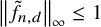 $ \left \lVert {\tilde {f}_{n,d}} \right \rVert _\infty \leq 1$
such that
$ \left \lVert {\tilde {f}_{n,d}} \right \rVert _\infty \leq 1$
such that
 $$\begin{align*}\left\lvert { a_0+a_1+\ldots+a_n } \right\rvert = \left( { 1 - O \left\{ { n^3 \exp \left( {-\frac{d}{5n}} \right) } \right\} } \right) \sum_{\nu=0}^n \binom{-1/2}{\nu}^2. \end{align*}$$
On combining this with Theorem 1.2 we immediately deduce the following result:
Corollary 2.2.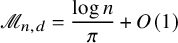 $\displaystyle \mathscr {M}_{n,d} = \frac {\log n}{\pi } + O(1) $
for
$\displaystyle \mathscr {M}_{n,d} = \frac {\log n}{\pi } + O(1) $
for $d> 16 \mkern 2mu n \log n$
and
$d> 16 \mkern 2mu n \log n$
and $n\to \infty $
.
$n\to \infty $
.
Newman [Reference Newman11, p. 187] also remarks that by (1.5) and (1.2) one has
 $$\begin{align*}\mathscr{M}_{n,d} \leq \frac{\log d}{\pi} + O(1), \end{align*}$$
and proceeds to ask whether ‘[the left hand side] ever gets this large’ (as n varies from $0$
to
$0$
to $d-1$
). He points out that (1.7) answers this in the affirmative. We remark that our Corollary 2.2 furnishes the following estimate:
$d-1$
). He points out that (1.7) answers this in the affirmative. We remark that our Corollary 2.2 furnishes the following estimate:
Corollary 2.3. $\displaystyle \mathscr {M}_{n,d} = \frac {\log d}{\pi } + O(\log \log d) $
provided that
$\displaystyle \mathscr {M}_{n,d} = \frac {\log d}{\pi } + O(\log \log d) $
provided that $\displaystyle n \asymp \frac {d}{\log d} $
.
$\displaystyle n \asymp \frac {d}{\log d} $
.
This may be regarded as another positive answer to Newman’s question up to lower order terms.
Remark 2.4 (Improvements to the error terms)
We have refrained from attempting to get the sharpest error term in Theorem 2.1 that our method allows for. Also the number $16 \;(>3\cdot 5)$
in Corollary 2.2 is not optimal in this regard. It would be particularly pleasing if Corollary 2.2 could be established for
$16 \;(>3\cdot 5)$
in Corollary 2.2 is not optimal in this regard. It would be particularly pleasing if Corollary 2.2 could be established for $d\gg n$
, but we do not know if this can be achieved. We refer to §5.4 below for further discussion pertaining to potential improvements.
$d\gg n$
, but we do not know if this can be achieved. We refer to §5.4 below for further discussion pertaining to potential improvements.
2.2 Exact formulæ
Before stating further results, let us provide more context. Shapiro [Reference Shapiro19] also considers extremal problems for more general sums than in (1.1), namely the question of maximising
 $$ \begin{align} \left\lvert { t_0 a_0 + \ldots + t_{d-1} a_{d-1} } \right\rvert \end{align} $$
over all polynomials $f = \sum _\nu a_\nu X^\nu \in {\mathbb {C}}[X]^{<d}$
with
$f = \sum _\nu a_\nu X^\nu \in {\mathbb {C}}[X]^{<d}$
with $ \left \lVert {f} \right \rVert _\infty \leq 1$
, where
$ \left \lVert {f} \right \rVert _\infty \leq 1$
, where $\boldsymbol {t} = (t_0,\ldots ,t_{d-1})\in {\mathbb {C}}^d$
is fixed. The outcome of his theory is a better theoretical understanding of the behaviour of the extremal polynomials (for the above maximisation problem) on the unit circle. In particular, for those
$\boldsymbol {t} = (t_0,\ldots ,t_{d-1})\in {\mathbb {C}}^d$
is fixed. The outcome of his theory is a better theoretical understanding of the behaviour of the extremal polynomials (for the above maximisation problem) on the unit circle. In particular, for those $\boldsymbol {t}$
for which the extremal polynomials are not given by monomials, he finds that for some
$\boldsymbol {t}$
for which the extremal polynomials are not given by monomials, he finds that for some $r\leq d$
there are complex numbers
$r\leq d$
there are complex numbers $z_1,\ldots ,z_r, u_1,\ldots ,u_r$
with
$z_1,\ldots ,z_r, u_1,\ldots ,u_r$
with $ \left \lvert {z_1} \right \rvert = \ldots = \left \lvert {z_r} \right \rvert = 1$
such that
$ \left \lvert {z_1} \right \rvert = \ldots = \left \lvert {z_r} \right \rvert = 1$
such that
 $$ \begin{align} t_0 a_0 + \ldots + t_{d-1} a_{d-1} = \sum_{\nu=1}^r u_\nu f(z_\nu) \end{align} $$
for all f as above, and the answer to the maximisation of (2.1) is given exactly by $ \left \lvert {u_1} \right \rvert +\ldots + \left \lvert {u_r} \right \rvert $
(see [Reference Shapiro19, §§ 2.3–4]).
$ \left \lvert {u_1} \right \rvert +\ldots + \left \lvert {u_r} \right \rvert $
(see [Reference Shapiro19, §§ 2.3–4]).
In Shapiro’s terminology, the $z_\nu $
are called the nodes associated to the functional given by
$z_\nu $
are called the nodes associated to the functional given by $\boldsymbol {t}$
. Observe that (2.2) may be interpreted as decomposing said functional using point evaluations at the
$\boldsymbol {t}$
. Observe that (2.2) may be interpreted as decomposing said functional using point evaluations at the $z_\nu $
(see also (6.5) below), yet there may be many more such decompositions with point evaluations not at the nodes. Despite this promising insight, Shapiro notes that ‘[he] has been unable to devise any method for finding the nodes’ ([Reference Shapiro19, § 2.4 2]).Footnote
1
$z_\nu $
(see also (6.5) below), yet there may be many more such decompositions with point evaluations not at the nodes. Despite this promising insight, Shapiro notes that ‘[he] has been unable to devise any method for finding the nodes’ ([Reference Shapiro19, § 2.4 2]).Footnote
1
Here we point out that Newman’s method [Reference Newman11] furnishes a (thin) host of examples for which the nodes can be computed. The next theorem (proved in §6.3 below) follows rather easily from a careful reading of Newman’s argument:Footnote 2
Theorem 2.5. Let n and d be positive integers such that $d\geq 2n-1$
. Moreover, let
$d\geq 2n-1$
. Moreover, let
 $$\begin{align*}\boldsymbol{t}^n = (t_{0\bmod 2n},\ldots,t_{n-1\bmod 2n}) \in {\mathbb{C}}^n \end{align*}$$
be arbitrary. Let $t_{n+\nu \bmod 2n} = - t_{\nu \bmod 2n}$
for
$t_{n+\nu \bmod 2n} = - t_{\nu \bmod 2n}$
for $\nu =0,\ldots ,n-1$
. Then, for every polynomial
$\nu =0,\ldots ,n-1$
. Then, for every polynomial $f = \sum _\nu a_\nu X^\nu \in {\mathbb {C}}[X]^{<d}$
with
$f = \sum _\nu a_\nu X^\nu \in {\mathbb {C}}[X]^{<d}$
with $ \left \lVert {f} \right \rVert _\infty \leq 1$
, one has
$ \left \lVert {f} \right \rVert _\infty \leq 1$
, one has

Moreover, there is a choice of f as above for which ‘ $\leq $
’ in (2.3) is attained with equality. In fact, this f may even be chosen to have degree
$\leq $
’ in (2.3) is attained with equality. In fact, this f may even be chosen to have degree $\leq 2n-2$
.
$\leq 2n-2$
.
Remark. Evidently, Theorem 2.5 falls short of implying Theorem 1.3. Here the latter theorem corresponds to the choice $\boldsymbol {t} = (1,\ldots ,1,0,\ldots ,0) \in {\mathbb {C}}^d$
in (2.1), with equally many
$\boldsymbol {t} = (1,\ldots ,1,0,\ldots ,0) \in {\mathbb {C}}^d$
in (2.1), with equally many $1$
’s and
$1$
’s and $0$
’s. However, Theorem 2.5 does handle
$0$
’s. However, Theorem 2.5 does handle $\boldsymbol {t} = (1,\ldots ,1,-1,\ldots ,-1)$
and Newman [Reference Newman11] provides a rather ingenious argument for bridging this gap.
$\boldsymbol {t} = (1,\ldots ,1,-1,\ldots ,-1)$
and Newman [Reference Newman11] provides a rather ingenious argument for bridging this gap.
We note that the vectors $\boldsymbol {t}$
in (2.1) to which Theorem 2.5 applies are of the form
$\boldsymbol {t}$
in (2.1) to which Theorem 2.5 applies are of the form

where ‘ $/\!/\!/$
’ indicates that suitably many last few entries in the final block are to be omitted as to have
$/\!/\!/$
’ indicates that suitably many last few entries in the final block are to be omitted as to have $\boldsymbol {t}$
belong to
$\boldsymbol {t}$
belong to ${\mathbb {C}}^d$
. We are also able to prove the following variant of Theorem 2.5 which handles the more symmetric case of vectors
${\mathbb {C}}^d$
. We are also able to prove the following variant of Theorem 2.5 which handles the more symmetric case of vectors $\boldsymbol {t}$
of the form
$\boldsymbol {t}$
of the form

Theorem 2.6. Let n and d be positive integers such that $d\geq 2n-1$
. Moreover, let
$d\geq 2n-1$
. Moreover, let
 $$\begin{align*}\boldsymbol{t}^n = (t_{0\bmod n},\ldots,t_{n-1\bmod n}) \in {\mathbb{C}}^n \end{align*}$$
be arbitrary. Then, for every polynomial $f = \sum _\nu a_\nu X^\nu \in {\mathbb {C}}[X]^{<d}$
with
$f = \sum _\nu a_\nu X^\nu \in {\mathbb {C}}[X]^{<d}$
with $ \left \lVert {f} \right \rVert _\infty \leq 1$
, one has
$ \left \lVert {f} \right \rVert _\infty \leq 1$
, one has

Moreover, there is a choice of f as above for which ‘ $\leq $
’ in (2.4) is attained with equality. In fact, this f may even be chosen to have degree
$\leq $
’ in (2.4) is attained with equality. In fact, this f may even be chosen to have degree $\leq 2n-2$
.
$\leq 2n-2$
.
As an application of (either of) the two theorems we prove the following cute inequality:
Corollary 2.7. Let $0\leq k<n$
be integers. Then, for any polynomial
$0\leq k<n$
be integers. Then, for any polynomial $f\in {\mathbb {C}}[X]^{<2n+k}$
,
$f\in {\mathbb {C}}[X]^{<2n+k}$
,
 $$ \begin{align} \left\lvert {\frac{f^{(k)}(0)}{k!}} \right\rvert + \left\lvert {\frac{f^{(n+k)}(0)}{(n+k)!}} \right\rvert \leq \left\lVert {f} \right\rVert _\infty. \end{align} $$
Moreover, equality occurs for some polynomial of degree $\leq 2n-2$
.
$\leq 2n-2$
.
2.3 A general bound
In both Theorem 2.5 and Theorem 2.6 we are able to handle an n-dimensional subspace of functionals on ${\mathbb {C}}[X]^{<d}$
. Specifically for
${\mathbb {C}}[X]^{<d}$
. Specifically for

the sum of these subspaces turns out to be the whole dual space of ${\mathbb {C}}[X]^{<d}$
. The underlying reason is that (in the notation from §2.2) every vector
${\mathbb {C}}[X]^{<d}$
. The underlying reason is that (in the notation from §2.2) every vector $\boldsymbol {t}\in {\mathbb {C}}^d$
admits a decomposition of the form
$\boldsymbol {t}\in {\mathbb {C}}^d$
admits a decomposition of the form

for suitable vectors $\boldsymbol {t}_{+}^n, \boldsymbol {t}_{-}^n \in {\mathbb {C}}^n$
(see (6.11) below).
$\boldsymbol {t}_{+}^n, \boldsymbol {t}_{-}^n \in {\mathbb {C}}^n$
(see (6.11) below).
In general, this does not, unfortunately, enable us to obtain sharp bounds for (2.1). However, we still get upper bounds:
Corollary 2.8. Let d be a positive integer and write $D = d$
or
$D = d$
or $=d-1$
according to whether d is even or odd. Let
$=d-1$
according to whether d is even or odd. Let $\boldsymbol {t} = (t_0,\ldots ,t_{d-1}) \in {\mathbb {C}}^d$
be arbitrary. Then, for every polynomial
$\boldsymbol {t} = (t_0,\ldots ,t_{d-1}) \in {\mathbb {C}}^d$
be arbitrary. Then, for every polynomial $f = \sum _\nu a_\nu X^\nu \in {\mathbb {C}}[X]^{<d}$
with
$f = \sum _\nu a_\nu X^\nu \in {\mathbb {C}}[X]^{<d}$
with $ \left \lVert {f} \right \rVert _\infty \leq 1$
, one has
$ \left \lVert {f} \right \rVert _\infty \leq 1$
, one has

Lastly, let us use Shapiro’s example (1.1) as a benchmark for Corollary 2.8.
Remark 2.9. For $d=2n$
and
$d=2n$
and $\boldsymbol {t} = (1_{\times n},0_{\times n}) \in {\mathbb {C}}^d$
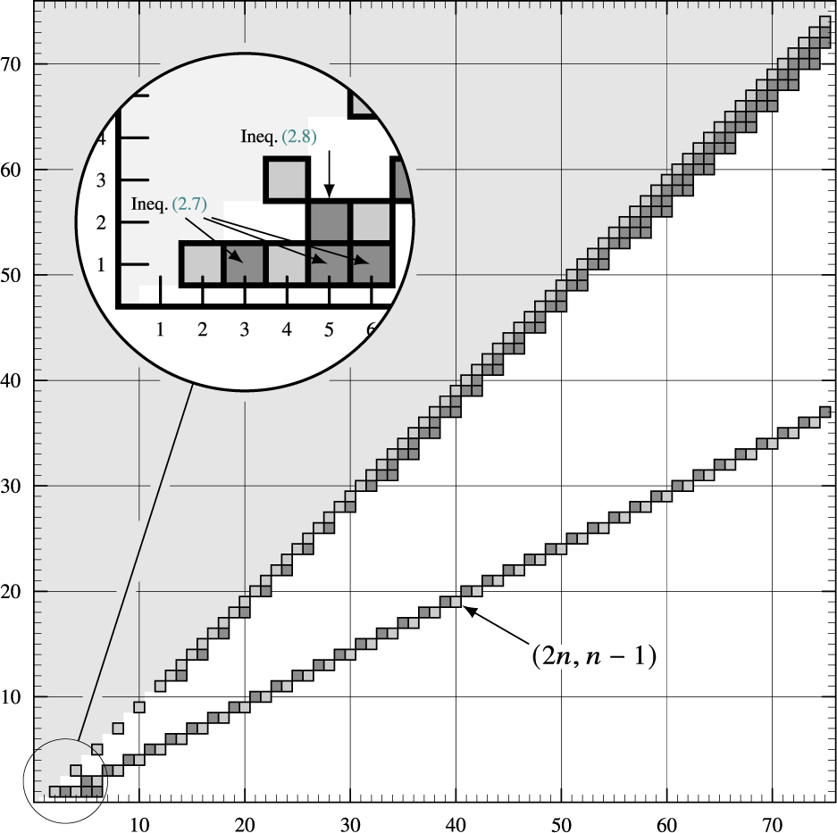
the right hand side (2.6) turns out to be precisely Newman’s bound (1.6). However, we cannot quite deduce Newman’s result (Theorem 1.3) from Corollary 2.8, because our bound (2.6) is not guaranteed to be sharp. The fact that the bound (2.6) may indeed fail to be sharp can be seen from the next example (namely the fact that there are white parts in Figure 1).
$\boldsymbol {t} = (1_{\times n},0_{\times n}) \in {\mathbb {C}}^d$
the right hand side (2.6) turns out to be precisely Newman’s bound (1.6). However, we cannot quite deduce Newman’s result (Theorem 1.3) from Corollary 2.8, because our bound (2.6) is not guaranteed to be sharp. The fact that the bound (2.6) may indeed fail to be sharp can be seen from the next example (namely the fact that there are white parts in Figure 1).
A numerical experiment showing when Corollary 2.8 produces stronger upper bounds on the maximum $\mathscr {M}_{n,d}$
from Problem 1.1 than previously known (cf. Example 2.10). The plot shows the points
$\mathscr {M}_{n,d}$
from Problem 1.1 than previously known (cf. Example 2.10). The plot shows the points $(d,n)$
,
$(d,n)$
, $0\leq n<d\leq 75$
, for which the upper bound (2.6) furnished by Corollary 2.8 for
$0\leq n<d\leq 75$
, for which the upper bound (2.6) furnished by Corollary 2.8 for $\boldsymbol {t} = (1_{\times (n+1)},0_{\times (d-n-1)}) \in {\mathbb {C}}^d$
is strictly smaller than the bound
$\boldsymbol {t} = (1_{\times (n+1)},0_{\times (d-n-1)}) \in {\mathbb {C}}^d$
is strictly smaller than the bound $\mathscr {L}_n$
for
$\mathscr {L}_n$
for $\mathscr {M}_{n,d}$
coming from Landau’s theorem (see (1.5)).
$\mathscr {M}_{n,d}$
coming from Landau’s theorem (see (1.5)).

Example 2.10. Using a computer, we have investigated when Corollary 2.8 yields non-trivial information about (1.5): for $0\leq n<d\leq 75$
we have computed the upper bound (2.6) (
$0\leq n<d\leq 75$
we have computed the upper bound (2.6) ( $\mathscr {C}_{n,d}$
say) furnished by Corollary 2.8 for
$\mathscr {C}_{n,d}$
say) furnished by Corollary 2.8 for $\boldsymbol {t} = (1_{\times (n+1)},0_{\times (d-n-1)}) \in {\mathbb {C}}^d$
. For instance, we obtain the following (hitherto unknown) upper bounds for
$\boldsymbol {t} = (1_{\times (n+1)},0_{\times (d-n-1)}) \in {\mathbb {C}}^d$
. For instance, we obtain the following (hitherto unknown) upper bounds for $\mathscr {M}_{1,d}$
(
$\mathscr {M}_{1,d}$
( $d=3,5,6$
):
$d=3,5,6$
):
 $$ \begin{align} \left. \begin{array}{ @{} r @{}c@{} l @{}c@{} c@{}c@{} l } \mathscr{M}_{1,3} &{}\leq{}& \mathscr{C}_{1,3} &{} = {}& \smash{ \tfrac{1}{2} + \tfrac{1}{\sqrt{2}} } &{} = {}& 1.2071\ldots \\[3pt] \mathscr{M}_{1,5} &{}\leq{}& \mathscr{C}_{1,5} &{} = {}& \smash{ \tfrac{2}{3} + \tfrac{1}{\sqrt{3}} } &{} = {}& 1.2440\ldots \\[3pt] \mathscr{M}_{1,6} &{}\leq{}& \mathscr{C}_{1,6} &{} = {}& \smash{ \tfrac{2}{3} + \tfrac{1}{\sqrt{3}} } \end{array} \right\rbrace < 1.25 = \tfrac{5}{4} = \mathscr{L}_1. \end{align} $$
Furthermore, we have
 $$ \begin{align} \mathscr{M}_{2,5} \leq \mathscr{C}_{2,5} = \tfrac{4}{3} = 1.3\dot{3} < 1.390625 = \tfrac{89}{64} = \mathscr{L}_2. \end{align} $$
Figutre 1 shows the tuples $(d,n)$
for which
$(d,n)$
for which $\mathscr {C}_{n,d} < \mathscr {L}_n$
. Note that we have the trivial cases
$\mathscr {C}_{n,d} < \mathscr {L}_n$
. Note that we have the trivial cases $\mathscr {M}_{0,d} = \mathscr {M}_{d-1,d} = 1$
, and
$\mathscr {M}_{0,d} = \mathscr {M}_{d-1,d} = 1$
, and $\mathscr {M}_{n-1,2n}$
is already covered by Newman’s result (recall Remark 2.9, though). In the figure we have greyed these out.
$\mathscr {M}_{n-1,2n}$
is already covered by Newman’s result (recall Remark 2.9, though). In the figure we have greyed these out.
3 Plan of the paper
In §4 we show that Landau’s bound (1.2) is not sharp for polynomials. In §5 we prove Theorem 2.1. The key result in our approach turns out to be a ‘quantitative Eneström–Kakeya theorem’, stated as Theorem 5.4 below. In §6 we extend Newman’s approach. The key outcome of this is given as Corollary 6.5 below. In §6.3, we use that result to prove Theorem 2.5 and Theorem 2.6. Finally, in §6.4 we prove the two corollaries enunciated in §2.2 and §2.3.
Let us also mention a few points about notation: we use both the Landau symbol $O(\,\cdot \,)$
and Vinogradov’s notation
$O(\,\cdot \,)$
and Vinogradov’s notation $\ll $
in the usual fashion. The implicit constants are always absolute, unless the contrary is explicitly indicated using subscripts (see, e.g., (5.2)).
$\ll $
in the usual fashion. The implicit constants are always absolute, unless the contrary is explicitly indicated using subscripts (see, e.g., (5.2)).
4 Polynomials and Landau’s bound
4.1 Landau’s argument
In this section we give a self-contained proof that Landau’s bound (1.2) is not sharp for polynomials. Of course, this result is not new. In fact, it follows directly from Landau’s characterisation of the extremal functions in Theorem 1.2 (see [Reference Landau8], but not [Reference Landau9], where the required characterisation is omitted). Nevertheless, we believe that revisiting Landau’s argument is instructive. We return to this point in §4.2 below.
Proposition 4.1. Let $d>n\geq 1$
be integers. Then there is some
$d>n\geq 1$
be integers. Then there is some $\delta (n,d)>0$
such that for every polynomial
$\delta (n,d)>0$
such that for every polynomial $f = \sum _\nu a_\nu X^\nu \in {\mathbb {C}}[X]^{<d}$
with
$f = \sum _\nu a_\nu X^\nu \in {\mathbb {C}}[X]^{<d}$
with $ \left \lVert {f} \right \rVert _\infty \leq 1$
, one has
$ \left \lVert {f} \right \rVert _\infty \leq 1$
, one has
 $$ \begin{align} \left\lvert { a_0+a_1+\ldots+a_n } \right\rvert \leq \sum_{\nu=0}^n \binom{-1/2}{\nu}^2 \mkern-3mu - \delta(n,d). \end{align} $$
Proof. By compactness of the unit ball in $({\mathbb {C}}[X]^{<d}, \left \lVert {\,\cdot \,} \right \rVert _\infty )$
, there exists a polynomial
$({\mathbb {C}}[X]^{<d}, \left \lVert {\,\cdot \,} \right \rVert _\infty )$
, there exists a polynomial $f = \sum _\nu a_\nu X^\nu \in {\mathbb {C}}[X]^{<d}$
with
$f = \sum _\nu a_\nu X^\nu \in {\mathbb {C}}[X]^{<d}$
with $ \left \lVert {f} \right \rVert _\infty \leq 1$
for which (1.2) is maximal. Let f be such a polynomial. Furthermore, let
$ \left \lVert {f} \right \rVert _\infty \leq 1$
for which (1.2) is maximal. Let f be such a polynomial. Furthermore, let $P_n$
be given as in (1.4). Then, by means of comparison with the binomial series expansion
$P_n$
be given as in (1.4). Then, by means of comparison with the binomial series expansion

it follows that
 $$\begin{align*}P_n^2(z) = 1 + z + z^2 + \ldots + z^n + \text{terms of higher order} \quad(\text{for } z\in{\mathbb{C}}), \end{align*}$$
so that Cauchy’s formula, trivial estimation and Parseval’s identity yield

Therefore, in order to establish the existence of $\delta (n,d)>0$
as in (4.1), it suffices to observe that ‘
$\delta (n,d)>0$
as in (4.1), it suffices to observe that ‘ $\leq $
’ in (4.2) actually holds with ‘
$\leq $
’ in (4.2) actually holds with ‘ $<$
’. This is simple, for if we had equality in (4.2) then
$<$
’. This is simple, for if we had equality in (4.2) then $ \left \lvert {f(z)} \right \rvert = 1$
for all
$ \left \lvert {f(z)} \right \rvert = 1$
for all $ \left \lvert {z} \right \rvert =1$
(in the first place, at least at the points z,
$ \left \lvert {z} \right \rvert =1$
(in the first place, at least at the points z, $ \left \lvert {z} \right \rvert =1$
, where
$ \left \lvert {z} \right \rvert =1$
, where $P_n$
does not vanish,Footnote
3
but then for all
$P_n$
does not vanish,Footnote
3
but then for all $ \left \lvert {z} \right \rvert =1$
by reason of continuity). However, this can only happen if f is a monomal (see Lemma 4.3 below); yet in this case
$ \left \lvert {z} \right \rvert =1$
by reason of continuity). However, this can only happen if f is a monomal (see Lemma 4.3 below); yet in this case $ \left \lvert { a_0 + a_1 + \ldots + a_n } \right \rvert = \left \lVert {f} \right \rVert_{\infty} = 1$
, but the right hand side of (1.2) is
$ \left \lvert { a_0 + a_1 + \ldots + a_n } \right \rvert = \left \lVert {f} \right \rVert_{\infty} = 1$
, but the right hand side of (1.2) is $>1$
.
$>1$
.
Remark 4.2. It follows from a general result of Shapiro, [Reference Shapiro19, Theorem 13 in § 2.7], that $\delta (n,d)\to 0$
for fixed n and
$\delta (n,d)\to 0$
for fixed n and $d\to \infty $
. Our Theorem 2.1 relaxes the condition on n.
$d\to \infty $
. Our Theorem 2.1 relaxes the condition on n.
The following result (used in the proof of Proposition 4.1) is a special case of the well-known classification of rational functions of modulus one on the unit circle (see, e.g., [Reference Rudin17, Ch. 14, Ex. 3 on p. 293]). We include a proof (without any claim of novelty) both for completeness’ sake and for lack of a suitable reference.
Lemma 4.3. Let $f\in {\mathbb {C}}[X]$
be a polynomial such that
$f\in {\mathbb {C}}[X]$
be a polynomial such that $ \left \lvert {f(z)} \right \rvert =1$
for all
$ \left \lvert {f(z)} \right \rvert =1$
for all $z\in {\mathbb {C}}$
with
$z\in {\mathbb {C}}$
with $ \left \lvert {z} \right \rvert =1$
. Then f is a monomial.
$ \left \lvert {z} \right \rvert =1$
. Then f is a monomial.
Proof. Let $\bar {f}$
be the polynomial obtained from f by replacing each coefficient by its complex conjugate. For
$\bar {f}$
be the polynomial obtained from f by replacing each coefficient by its complex conjugate. For $ \left \lvert {z} \right \rvert =1$
we have
$ \left \lvert {z} \right \rvert =1$
we have $\overline {z} = 1/z$
. Consequently, the rational function
$\overline {z} = 1/z$
. Consequently, the rational function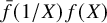 $\bar {f}(1/X) f(X)$
equals one: (a) on the unit circle and, a fortiori, (b) everywhere (by the identity principle, for instance). Now if f were to have a non-zero root
$\bar {f}(1/X) f(X)$
equals one: (a) on the unit circle and, a fortiori, (b) everywhere (by the identity principle, for instance). Now if f were to have a non-zero root $z\in {\mathbb {C}}$
, then we reap the contradiction
$z\in {\mathbb {C}}$
, then we reap the contradiction $1 = \bar {f}(1/z) f(z) = 0$
. Hence, the zero locus of f is either
$1 = \bar {f}(1/z) f(z) = 0$
. Hence, the zero locus of f is either $\emptyset $
or
$\emptyset $
or
 . In both cases, it follows that f is a monomial.
4.2 Reflections on Landau’s argument
The key to Proposition 4.1 may be described as resting on two observations:
-
1. The expression in question, $a_0+a_1+\ldots +a_n$
, admits a nice integral representation, namely (4.3)
$a_0+a_1+\ldots +a_n$
, admits a nice integral representation, namely (4.3) -
2. The ‘integration kernel’
$1 + z + z^2 + \ldots + z^n$
in (4.3) can be replaced by
$P_n^2(z)$
(recall (4.2)). In the holomorphic case (Theorem 1.2) one can, in fact, use this to get sharp bounds via the functions
$f_n$
given in (1.4).





It is clear that this approach does not readily generalise to determine the maximum $\mathscr {M}_{n,d}$
of the left hand side of (1.2) as f ranges over all
$\mathscr {M}_{n,d}$
of the left hand side of (1.2) as f ranges over all $1$
-bounded polynomials of degree
$1$
-bounded polynomials of degree $<d$
: what we lack is sufficient understanding of the precise boundary behaviour of the corresponding extremal polynomials f.
$<d$
: what we lack is sufficient understanding of the precise boundary behaviour of the corresponding extremal polynomials f.
Despite not having the required understanding of $f(z)$
for all
$f(z)$
for all $ \left \lvert {z} \right \rvert =1$
, it is possible to get control on a finite number of such z using an interpolation-based approach. In this way one can get results when the integral formula (4.3) can be replaced by a finite sum (involving point evaluations of f) with ‘especially few’ terms. Such phenomena of replacing integration of polynomials by finite sums with few terms is a well-known theme in numerical analysis, namely Gauss quadrature. In our case, this discrete analogue of (4.3) is given in the form of (6.5) in Corollary 6.5 below. We return to this in §6, when we discuss the exact formulæ presented in §2.2.
$ \left \lvert {z} \right \rvert =1$
, it is possible to get control on a finite number of such z using an interpolation-based approach. In this way one can get results when the integral formula (4.3) can be replaced by a finite sum (involving point evaluations of f) with ‘especially few’ terms. Such phenomena of replacing integration of polynomials by finite sums with few terms is a well-known theme in numerical analysis, namely Gauss quadrature. In our case, this discrete analogue of (4.3) is given in the form of (6.5) in Corollary 6.5 below. We return to this in §6, when we discuss the exact formulæ presented in §2.2.
5 Asymptotic estimates
5.1 Proof of Theorem 2.1
The strategy is to approximate Landau’s extremal function $f_n$
by polynomials; this natural idea is already found in [Reference Shapiro19, Theorem 13 in § 2.7], where it is applied to more general extremal problems. In the generality of the cited result, one cannot hope to achieve error bounds as explicit as the ones we obtain here. Our approach hinges upon bounding away the poles of
$f_n$
by polynomials; this natural idea is already found in [Reference Shapiro19, Theorem 13 in § 2.7], where it is applied to more general extremal problems. In the generality of the cited result, one cannot hope to achieve error bounds as explicit as the ones we obtain here. Our approach hinges upon bounding away the poles of $f_n$
from the unit disk (cf. Figure 2). To achieve this, we shall employ the well-known Eneström–Kakeya theorem [Reference Eneström4, Reference Kakeya7] (see also [Reference Borwein and Erdélyi2, p. 13]):
$f_n$
from the unit disk (cf. Figure 2). To achieve this, we shall employ the well-known Eneström–Kakeya theorem [Reference Eneström4, Reference Kakeya7] (see also [Reference Borwein and Erdélyi2, p. 13]):
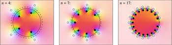
Zeros (black dots) and poles (white dots) of $f_n$
from (1.4) for
$f_n$
from (1.4) for
 . In each picture the two circles are centred about $0$
and have radii
$0$
and have radii $1$
and
$1$
and $1 + 1/(2n+1)$
, respectively.
$1 + 1/(2n+1)$
, respectively.

Lemma 5.1 (Eneström, 1893; Kakeya, 1912)
Let $a_n X^n + \ldots + a_1 X + a_0$
be a polynomial with positive coefficients
$a_n X^n + \ldots + a_1 X + a_0$
be a polynomial with positive coefficients $a_0 \geq a_1 \geq \ldots \geq a_n> 0$
. Then all its complex zeros are contained in the (closed) annulus with radii
$a_0 \geq a_1 \geq \ldots \geq a_n> 0$
. Then all its complex zeros are contained in the (closed) annulus with radii $\min Q$
and
$\min Q$
and $\max Q$
; here
$\max Q$
; here
 .
.
Corollary 5.2. The poles $\zeta \in {\mathbb {C}}$
of
$\zeta \in {\mathbb {C}}$
of $f_n$
given in (1.4) satisfy
$f_n$
given in (1.4) satisfy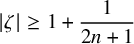 $\displaystyle \left \lvert {\zeta } \right \rvert \geq 1 + \frac {1}{2n+1} $
.
$\displaystyle \left \lvert {\zeta } \right \rvert \geq 1 + \frac {1}{2n+1} $
.
Proof. This follows from the definition (1.4) of $f_n$
, (1.3), Lemma 5.1, and
$f_n$
, (1.3), Lemma 5.1, and
 $$\begin{align*}- \binom{-1/2}{\nu} \bigg/ \binom{-1/2}{\nu+1} = \frac{2\nu+2}{2\nu+1}.\\[-42pt] \end{align*}$$
From the above one easily obtains decay estimates for the Taylor coefficients of the function $f_n$
. An unpleasant feature of this rather naïve approach is that it does not yield an explicit dependence on n. This is a nuisance for our purpose, which we mitigate in Proposition 5.5.
$f_n$
. An unpleasant feature of this rather naïve approach is that it does not yield an explicit dependence on n. This is a nuisance for our purpose, which we mitigate in Proposition 5.5.
Corollary 5.3. Fix an integer $n\geq 1$
and let
$n\geq 1$
and let
 $$ \begin{align} f_n(z) = \sum_{\nu=0}^\infty b_{n,\nu} z^\nu \end{align} $$
be the power series expansion (about the origin) of the rational function $f_n$
from (1.4). Then, for every
$f_n$
from (1.4). Then, for every $\epsilon \in (0,1)$
,
$\epsilon \in (0,1)$
,
 $$ \begin{align} b_{n,\nu} \ll_{n,\epsilon} \left( {1+\frac{1}{2n+1}-\epsilon} \right) ^{-\nu}. \end{align} $$
Proof. The radius R of convergence of the power series expansion (5.1) is precisely $\min _{\zeta } \mkern -2mu { \left \lvert {\zeta } \right \rvert }$
, where
$\min _{\zeta } \mkern -2mu { \left \lvert {\zeta } \right \rvert }$
, where $\zeta $
ranges over the poles of
$\zeta $
ranges over the poles of $f_n$
. The lemma now follows upon combining Corollary 5.2 and the well-known Cauchy–Hadamard formula for R.
$f_n$
. The lemma now follows upon combining Corollary 5.2 and the well-known Cauchy–Hadamard formula for R.
Proof of Theorem 2.1
Suppose for the moment that we had a version of (5.2) at our disposal in which the dependence of the implied constant was spelled out in terms of n. Precisely, we shall work with the inequality
 $$ \begin{align} \left\lvert {b_{n,\nu}} \right\rvert \ll n^2 \left( {1+\frac{1}{4n}} \right) ^{-\nu}. \end{align} $$
which we establish in Proposition 5.5 below.
We shall employ (5.3) to see how well the polynomial
 $$\begin{align*}f_{n,d} = \sum_{\nu=0}^{d-1} b_{n,\nu} X^\nu. \end{align*}$$
approximates $f_n$
(see (5.1)). Indeed, for all
$f_n$
(see (5.1)). Indeed, for all $ \left \lvert {z} \right \rvert \leq 1$
,
$ \left \lvert {z} \right \rvert \leq 1$
,

In particular,
 $$\begin{align*}\left\lVert {f_{n,d}} \right\rVert _\infty \leq \left\lVert {f_n} \right\rVert _\infty + O(E(n,d)) = 1 + O(E(n,d)). \end{align*}$$
Therefore, $\tilde {f}_{n,d} = f_{n,d} / \left \lVert {f_{n,d}} \right \rVert _\infty $
is a polynomial with
$\tilde {f}_{n,d} = f_{n,d} / \left \lVert {f_{n,d}} \right \rVert _\infty $
is a polynomial with $ \left \lVert {\tilde {f}_{n,d}} \right \rVert _\infty = 1$
. If
$ \left \lVert {\tilde {f}_{n,d}} \right \rVert _\infty = 1$
. If $d>n$
, then the first
$d>n$
, then the first $n+1$
coefficients of the polynomial
$n+1$
coefficients of the polynomial $f_{n,d}$
sum to the right hand side of (1.2). In particular, we have constructed a polynomial of degree
$f_{n,d}$
sum to the right hand side of (1.2). In particular, we have constructed a polynomial of degree $<d$
, bounded by
$<d$
, bounded by $1$
in absolute value on the unit disk, whose first
$1$
in absolute value on the unit disk, whose first $n+1$
coefficients sum to
$n+1$
coefficients sum to

in absolute value.
5.2 A quantitative Eneström–Kakeya theorem
For our desired explicit version of Corollary 5.3, the original Eneström–Kakeya theorem is insufficient. Fortunately, it is an easy matter to extract a suitable quantitative statement of the standard proof of said theorem. Despite its easy proof, we believe that the result obtained may be of independent interest:
Theorem 5.4 (Quantitative Eneström–Kakeya)
Let $p = a_n X^n + \ldots + a_1 X + a_0$
be a polynomial with positive coefficients
$p = a_n X^n + \ldots + a_1 X + a_0$
be a polynomial with positive coefficients $a_0 \geq a_1 \geq \ldots \geq a_n> 0$
. Let
$a_0 \geq a_1 \geq \ldots \geq a_n> 0$
. Let
 and put $r = \min Q \leq \max Q = R$
. Then, for
$r = \min Q \leq \max Q = R$
. Then, for
 , we have the following inequalities:
-
(1)
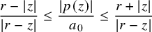
$\displaystyle \frac {r- \left \lvert {z} \right \rvert }{ \left \lvert {r-z} \right \rvert } \leq \frac { \left \lvert {p(z)} \right \rvert }{a_0} \leq \frac {r+ \left \lvert {z} \right \rvert }{ \left \lvert {r-z} \right \rvert } $
for
$ \left \lvert {z} \right \rvert \leq r$
, -
(2)
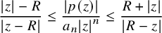
$\displaystyle \frac { \left \lvert {z} \right \rvert -R}{ \left \lvert {z-R} \right \rvert } \leq \frac { \left \lvert {p(z)} \right \rvert }{a_n \left \lvert {z} \right \rvert ^n} \leq \frac {R+ \left \lvert {z} \right \rvert }{ \left \lvert {R-z} \right \rvert } $
for
$ \left \lvert {z} \right \rvert \geq R$
.


Proof. (We follow [Reference Borwein and Erdélyi2, pp. 12–Reference Rack13] with minimal adjustments in order to extract the desired inequalities.) For $\zeta \in {\mathbb {C}}$
with
$\zeta \in {\mathbb {C}}$
with $ \left \lvert {\zeta } \right \rvert \leq 1$
we have
$ \left \lvert {\zeta } \right \rvert \leq 1$
we have
 $$ \begin{align} \begin{aligned} \left\lvert { (1-\zeta) p(r\zeta) - a_0 } \right\rvert & = \left\lvert { (ra_1-a_0)\zeta+\ldots+(ra_n-a_{n-1})r^{n-1}\zeta^n-a_nr^n\zeta^{n+1} } \right\rvert \\ & \leq (a_0-ra_1) \left\lvert {\zeta} \right\rvert +\ldots+(a_{n-1}-ra_n)r^{n-1} \left\lvert {\zeta} \right\rvert ^n+a_nr^n \left\lvert {\zeta} \right\rvert ^{n+1} \\ & \leq \left\lbrace { (a_0-ra_1)+\ldots+(a_{n-1}-ra_n)r^{n-1}+a_nr^n } \right\rbrace \left\lvert {\zeta} \right\rvert \\ & = a_0 \left\lvert {\zeta} \right\rvert. \end{aligned} \end{align} $$
Then $\zeta = z/r \: (\neq 1)$
satisfies
$\zeta = z/r \: (\neq 1)$
satisfies $ \left \lvert {\zeta } \right \rvert \leq 1$
and we find that
$ \left \lvert {\zeta } \right \rvert \leq 1$
and we find that
 $$\begin{align*}\left\lvert { (1-\zeta) p(r\zeta) } \right\rvert \geq a_0 (1- \left\lvert {\zeta} \right\rvert ) \quad\text{and}\quad \left\lvert { (1-\zeta) p(r\zeta) } \right\rvert \leq a_0 (1+ \left\lvert {\zeta} \right\rvert ). \end{align*}$$
This shows (1).
For (2) one considers $\zeta =z/R$
for
$\zeta =z/R$
for $ \left \lvert {z} \right \rvert \geq R$
and estimates
$ \left \lvert {z} \right \rvert \geq R$
and estimates
 $$\begin{align*}\left\lvert {(1-\zeta)p(R\zeta)+a_n(R\zeta)^n\zeta} \right\rvert \end{align*}$$
similarly as in (5.4).
5.3 Growth of the Taylor coefficients of Landau’s extremal functions
$f_{n,d}$

Recall that our proof of Theorem 2.1, given in §5.1, crucially hinges on a certain ‘upgrade’ of Corollary 5.3 in which the dependence of the bound (5.2) on n is made explicit (see (5.2)). We are now ready to prove this explicit version:
Proposition 5.5. Assume the hypotheses of Corollary 5.3. Then
 $$ \begin{align} \left\lvert {b_{n,\nu}} \right\rvert \ll n^2 \left( {1+\frac{1}{4n}} \right) ^{-\nu}. \end{align} $$
Proof. Recall that, by Corollary 5.2, $f_n$
is holomorphic in the open disk with radius
$f_n$
is holomorphic in the open disk with radius $r = 1 + 1/(2n+1)$
centred about the origin. Consequently, for any
$r = 1 + 1/(2n+1)$
centred about the origin. Consequently, for any $0 < \rho < r$
, Cauchy’s estimate for Taylor coefficients yields
$0 < \rho < r$
, Cauchy’s estimate for Taylor coefficients yields
 $$\begin{align*}\left\lvert {b_{n,\nu}} \right\rvert \leq \rho^{-\nu} \max_{ \left\lvert {z} \right\rvert =\rho} \left\lvert {f_n(z)} \right\rvert = \rho^{n-\nu} \max_{ \left\lvert {z} \right\rvert =\rho} \left\lvert {\frac{P_n(1/z)}{P_n(z)}} \right\rvert. \end{align*}$$
We take $\rho = 1 + 1/4n$
and estimate this further using Theorem 5.4. Then (5.5) follows easily.
$\rho = 1 + 1/4n$
and estimate this further using Theorem 5.4. Then (5.5) follows easily.
5.4 Remark on the zeros of
$P_n$

As we have seen, information on the location of the roots of $P_n$
is vital to our proof of Theorem 2.1. Precisely, we should like to have good lower bounds on the absolute value of the roots of
$P_n$
is vital to our proof of Theorem 2.1. Precisely, we should like to have good lower bounds on the absolute value of the roots of $P_n$
. Let
$P_n$
. Let

Then Corollary 5.2 tells us that $r(n) - 1 \gg 1/n$
. Towards the other extreme, we can give the following upper bound:
$r(n) - 1 \gg 1/n$
. Towards the other extreme, we can give the following upper bound:
Proposition 5.6. We have $\displaystyle r(n) \leq 1 + O \left( {\frac {\log n}{n}} \right) $
for
$\displaystyle r(n) \leq 1 + O \left( {\frac {\log n}{n}} \right) $
for $n\geq 2$
.
$n\geq 2$
.
Proof. (The proof is based on an observation we have learned from work by Erdős and Turán [Reference Erdős and Turán5, § 6].) Observe that
 $$\begin{align*}1 = \left\lvert {P_n(0)} \right\rvert = \left\lvert {\binom{-1/2}{n}} \right\rvert \mkern 2mu \prod_z { \left\lvert {0-z} \right\rvert } \geq \left\lvert {\binom{-1/2}{n}} \right\rvert \mkern 2mu r(n)^n, \end{align*}$$
where z ranges over all n roots of $P_n$
(taking multiplicity into accountFootnote
4
). The absolute value of the binomial coefficient above is asymptotic to
$P_n$
(taking multiplicity into accountFootnote
4
). The absolute value of the binomial coefficient above is asymptotic to $1/\sqrt {\pi n}$
(by Stirling’s formula; cf. [Reference Landau9, pp. 22–23]). In particular, we have the inequality
$1/\sqrt {\pi n}$
(by Stirling’s formula; cf. [Reference Landau9, pp. 22–23]). In particular, we have the inequality $r(n)^n \leq 2 \sqrt {\pi n} < n$
for all sufficiently large
$r(n)^n \leq 2 \sqrt {\pi n} < n$
for all sufficiently large $n> 4\pi $
. Hence, for those n,
$n> 4\pi $
. Hence, for those n,
 $$\begin{align*}r(n) < \exp \left( {\frac{\log n}{n}} \right) < 1 + \frac{\log n}{n}. \end{align*}$$
In particular, we have the bound claimed in the proposition for all $n\geq 2$
.
$n\geq 2$
.
Consequently, for $n\geq 2$
, we have
$n\geq 2$
, we have
 $$ \begin{align} \frac{1}{n} \ll r(n) - 1 \ll \frac{\log n}{n}. \end{align} $$
Based on some limited numerical evidence, one may be tempted to conjecture that the lower bound is closer to the truth; we have been unable to resolve this.
Open problem 5.7. Improve on either of the two bounds in (5.6) to the extent that one of the following two statements follows:
 $$\begin{align*}\limsup_{n\to\infty} (r(n)-1)n = \infty, \quad \liminf_{n\to\infty} \frac{(r(n)-1)n}{\log n} = 0. \end{align*}$$
Ideally, establish an asymptotic formula for $(r(n)-1)n$
as
$(r(n)-1)n$
as $n\to \infty $
.
$n\to \infty $
.
Remark 5.8. We mention two other interesting facts about the roots of $P_n$
:
$P_n$
:
-
1. they are all simple, as can be seen by applying the Eneström–Kakeya theorem to the derivative of
$P_n$
; -
2. every point on the unit circle is an accumulation point of zeros of
$P_n$
for n restricted to a suitable subsequence of the positive integers; this follows from a classical theorem of Jentzsch [Reference Jentzsch6] on sections of power series with finite radius of convergence (see also the subsequent influential refinements by Szegö [Reference Szegö20] and Erdős–Turán [Reference Erdős and Turán5], as well as the monography [Reference Andrievskii and Blatt1]).


6 Interpolation with roots of unity
This section is devoted to the proof of both Theorem 2.5 and Theorem 2.6. We handle both simultaneously. Throughout this section fix a positive integer n and let

In the sequel, $\omega $
,
$\omega $
, $\varpi $
and
$\varpi $
and $\xi $
will always denote elements of
$\xi $
will always denote elements of $\Omega $
. Occurrences of ‘
$\Omega $
. Occurrences of ‘ $\pm $
’ or ‘
$\pm $
’ or ‘ $\mp $
’ always refer to the sign chosen in (6.1).
$\mp $
’ always refer to the sign chosen in (6.1).
6.1 Lagrange interpolators for roots of unity
Write
 $$ \begin{align} L_{\Omega,\omega} = \prod_{\substack{ \varpi\in\Omega \\ \varpi\neq\omega }} \frac{X-\varpi}{\omega-\varpi} \end{align} $$
for the Lagrange interpolating polynomial with respect to $\Omega $
and
$\Omega $
and $\omega $
. Clearly, for
$\omega $
. Clearly, for $\varpi \in \Omega $
,
$\varpi \in \Omega $
,
 $$ \begin{align} L_{\Omega,\omega}(\varpi) = \begin{cases} 1 & \text{if } \varpi = \omega, \\ 0 & \text{if } \varpi \neq \omega. \\ \end{cases} \end{align} $$
The key observation is the following neat property of the Lagrange interpolators with respect to our special choice for $\Omega $
:
$\Omega $
:
Proposition 6.1.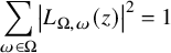 $\displaystyle \sum _{\omega \in \Omega } \left \lvert {L_{\Omega ,\omega }(z)} \right \rvert ^2 = 1 $
for all
$\displaystyle \sum _{\omega \in \Omega } \left \lvert {L_{\Omega ,\omega }(z)} \right \rvert ^2 = 1 $
for all $z\in {\mathbb {C}}$
with
$z\in {\mathbb {C}}$
with $ \left \lvert {z} \right \rvert =1$
.
$ \left \lvert {z} \right \rvert =1$
.
Remarks.
-
1. Proposition 6.1 for ‘
$+$
’ in the definition of
$\Omega $
is precisely Lemma 2 of [Reference Newman11]. -
2. Proposition 6.1 is the crucial ingredient for obtaining Corollary 6.5 below. The latter result is, as we shall see, a common generalization of Theorem 2.5 and Theorem 2.6.
-
3. The statement of Proposition 6.1 may become invalid if
$\Omega $
from (6.1) is replaced by some other set, even if that set consists only of roots of unity. For instance, for
, one easily checks that
$2 \sum _{\omega \in \Omega } \left \lvert {L_{\Omega ,\omega }(z)} \right \rvert ^2 = \left \lvert {z-1} \right \rvert ^2+ \left \lvert {z-{\mathrm {i}}} \right \rvert ^2$
. It would seem desirable to have a characterisation of the sets
$\Omega $
for which Proposition 6.1 holds.




We base the proof of Proposition 6.1 on three lemmas.
Lemma 6.2.
-
(1)
$\displaystyle \mp \frac {n}{\omega } = \prod _{\substack { \varpi \in \Omega \\ \varpi \neq \omega }} (\omega -\varpi ) $
, -
(2)
.

 .
.Proof. The first statement is certainly classical (see, e.g., [Reference Pólya and Szegő12, VI, § 9, Problem 74]); it follows from

Likewise, the second statement follows from a similar evaluation of the second derivative of $X^n\pm 1$
at
$X^n\pm 1$
at $\omega \in \Omega $
.
$\omega \in \Omega $
.
Lemma 6.3.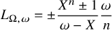 $\displaystyle L_{\Omega ,\omega } = \pm \frac {X^n\pm 1}{\omega -X} \frac {\omega }{n} $
in
$\displaystyle L_{\Omega ,\omega } = \pm \frac {X^n\pm 1}{\omega -X} \frac {\omega }{n} $
in ${\mathbb {C}}(X)$
.
${\mathbb {C}}(X)$
.
Proof. The product over the denominators in (6.2) is $\mp \omega /n$
by Lemma 6.2 (1). On the other hand, clearly, the product over the numerators equals
$\mp \omega /n$
by Lemma 6.2 (1). On the other hand, clearly, the product over the numerators equals $(X^n-1)/(X-\omega )$
. This establishes the lemma.
$(X^n-1)/(X-\omega )$
. This establishes the lemma.
Lemma 6.4.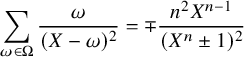 $\displaystyle \sum _{\omega \in \Omega } \frac {\omega }{(X-\omega )^2} = \mp \frac {n^2 X^{n-1}}{(X^n\pm 1)^2} $
in
$\displaystyle \sum _{\omega \in \Omega } \frac {\omega }{(X-\omega )^2} = \mp \frac {n^2 X^{n-1}}{(X^n\pm 1)^2} $
in ${\mathbb {C}}(X)$
.
${\mathbb {C}}(X)$
.
Proof. The claimed identity clearly follows from the polynomial identity
 $$ \begin{align} \sum_{\omega\in\Omega} \omega \prod_{\substack{ \varpi\in\Omega \\ \varpi\neq\omega }} (X-\varpi)^2 = \mp n^2 X^{n-1}. \end{align} $$
upon dividing both sides by $(X^n\pm 1)^2 = \prod _{\omega \in \Omega } (X-\omega )^2$
.
$(X^n\pm 1)^2 = \prod _{\omega \in \Omega } (X-\omega )^2$
.
In order to establish (6.4), observe that both sides equal one another for all $\omega \in \Omega $
, by virtue of Lemma 6.2 (1). Furthermore, also the derivatives of both sides of (6.4) are equal for all
$\omega \in \Omega $
, by virtue of Lemma 6.2 (1). Furthermore, also the derivatives of both sides of (6.4) are equal for all $\omega \in \Omega $
: indeed, we have
$\omega \in \Omega $
: indeed, we have

where the last equality follows from (both parts of) Lemma 6.2. Hence, the difference of both sides of (6.4) either vanishes or is a polynomial of degree $\geq 2n-1$
. Evidently, the latter is not the case, so we have (6.4).
$\geq 2n-1$
. Evidently, the latter is not the case, so we have (6.4).
Proof of Proposition 6.1
Clearly, we may suppose that $z\notin \Omega $
(by (6.3) or by continuity, for instance). Since
$z\notin \Omega $
(by (6.3) or by continuity, for instance). Since $ \left \lvert {z} \right \rvert =1$
, it holds that
$ \left \lvert {z} \right \rvert =1$
, it holds that $\overline {z} = 1/z$
. Thus, by Lemma 6.3,
$\overline {z} = 1/z$
. Thus, by Lemma 6.3,
 $$\begin{align*}\sum_{\omega\in\Omega} \left\lvert {L_{\Omega,\omega}(z)} \right\rvert ^2 = \sum_{\omega\in\Omega} \frac{z^n\pm1}{\omega-z} \frac{\omega}{n} \frac{z^{-n}\pm1}{\omega^{-1}-z^{-1}} \frac{\omega^{-1}}{n} = \mp \frac{(z^n\pm1)^2}{n^2 z^{n-1}} \sum_{\omega\in\Omega} \frac{\omega}{(z-\omega)^2}. \end{align*}$$
The result is now immediate from Lemma 6.4.
6.2 Application to functionals: the key result
In the sequel, we shall write  for the evaluation-at- $\omega $
functional
$\omega $
functional ${\mathbb {C}}[X]\to {\mathbb {C}}$
, mapping every polynomial f to
${\mathbb {C}}[X]\to {\mathbb {C}}$
, mapping every polynomial f to $f(\omega )$
. Proposition 6.1 now affords a proof of the following result which turns out to be nothing but a unified version of Theorem 2.5 and Theorem 2.6:
$f(\omega )$
. Proposition 6.1 now affords a proof of the following result which turns out to be nothing but a unified version of Theorem 2.5 and Theorem 2.6:
Corollary 6.5. Let n and $\Omega $
be as above and let
$\Omega $
be as above and let $d \geq 2n-1$
be an arbitrary integer. Let
$d \geq 2n-1$
be an arbitrary integer. Let $\ell \colon {\mathbb {C}}[X]^{<d} \to {\mathbb {C}}$
be a functional of the form
$\ell \colon {\mathbb {C}}[X]^{<d} \to {\mathbb {C}}$
be a functional of the form

with scalars $u_\omega \in {\mathbb {C}}$
. Then the norm
$u_\omega \in {\mathbb {C}}$
. Then the norm

of $\ell $
is given by
$\ell $
is given by
 $$\begin{align*}\left\lVert {\ell} \right\rVert = \sum_{\omega\in\Omega} \left\lvert { u_\omega } \right\rvert. \end{align*}$$
Proof. Let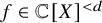 $f\in {\mathbb {C}}[X]^{<d}$
satisfy
$f\in {\mathbb {C}}[X]^{<d}$
satisfy $ \left \lVert {f} \right \rVert _\infty = 1$
. Certainly,
$ \left \lVert {f} \right \rVert _\infty = 1$
. Certainly,
 $$\begin{align*}\left\lvert {\ell(f)} \right\rvert \leq \sum_{\omega\in\Omega} \left\lvert {u_\omega} \right\rvert \left\lvert {f(\omega)} \right\rvert \leq \sum_{\omega\in\Omega} \left\lvert {u_\omega} \right\rvert , \end{align*}$$
so it suffices to produce an f with $ \left \lVert {f} \right \rVert _\infty = 1$
for which the above inequalities hold as equalities. Such an f is furnished by
$ \left \lVert {f} \right \rVert _\infty = 1$
for which the above inequalities hold as equalities. Such an f is furnished by
 $$\begin{align*}f = \sideset{}{^\star}\sum_{\omega\in\Omega} \frac{\overline{u_\omega}}{ \left\lvert {u_\omega} \right\rvert } L_{\Omega,\omega}^2, \end{align*}$$
where $\sum ^\star $
indicates that terms with
$\sum ^\star $
indicates that terms with $u_\omega = 0$
ought to be omitted. Indeed, since each
$u_\omega = 0$
ought to be omitted. Indeed, since each $L_{\Omega ,\omega }^2$
has degree
$L_{\Omega ,\omega }^2$
has degree $2n-2 < d$
, the degree of f is no higher than that. Moreover,
$2n-2 < d$
, the degree of f is no higher than that. Moreover, $ \left \lVert {f} \right \rVert _\infty = 1$
by Proposition 6.1, and (6.3) shows that
$ \left \lVert {f} \right \rVert _\infty = 1$
by Proposition 6.1, and (6.3) shows that
 $$\begin{align*}\ell(f) = \sideset{}{^\star}\sum_{\omega\in\Omega} \frac{\overline{u_\omega}}{ \left\lvert {u_\omega} \right\rvert } u_\omega = \sum_{\omega\in\Omega} \left\lvert {u_\omega} \right\rvert.\\[-50pt] \end{align*}$$
Remark 6.6. In §2.2 we have already noted that the idea of maximising certain functionals by relating them to point evaluation functionals is crucial in [Reference Shapiro19, Reference Newman11]. The interested reader is also referred to [Reference Rogosinski16] for general reflections on such an approach or, e.g., [Reference Rivlin15, Ch. 2.B] for further examples.
6.3 Application to functionals: cosmetic surgery
The functionals $\ell $
to which Corollary 6.5 applies are given in (6.5) in terms of point evaluation functionals. For applications to (2.1) we should rather like to describe these functionals in terms of their action on monomials. This is a staight-forward exercise in linear algebra and is the object of the present subsection.
$\ell $
to which Corollary 6.5 applies are given in (6.5) in terms of point evaluation functionals. For applications to (2.1) we should rather like to describe these functionals in terms of their action on monomials. This is a staight-forward exercise in linear algebra and is the object of the present subsection.
Lemma 6.7. A linear functional $\ell \colon {\mathbb {C}}[X]^{<d}\to {\mathbb {C}}$
is of the form (6.5) if and only if
$\ell \colon {\mathbb {C}}[X]^{<d}\to {\mathbb {C}}$
is of the form (6.5) if and only if $(u_\omega )_{\omega \in \Omega }$
satisfies the following system of linear equations:
$(u_\omega )_{\omega \in \Omega }$
satisfies the following system of linear equations:
 $$ \begin{align} \sum_{\omega\in\Omega} u_\omega \omega^\kappa = \ell(X^\kappa), \quad0\leq\kappa<d. \end{align} $$
Proof. Consider the spaces $V = {\mathbb {C}}[X]^{<n}$
and
$V = {\mathbb {C}}[X]^{<n}$
and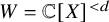 $W = {\mathbb {C}}[X]^{<d}$
. On V pick the basis
$W = {\mathbb {C}}[X]^{<d}$
. On V pick the basis
 and consider its dual basis
 (i.e., $x_\nu ^*(X^\eta ) = 1$
if
$x_\nu ^*(X^\eta ) = 1$
if $\nu =\eta $
and
$\nu =\eta $
and $=0$
otherwise). Construct a basis
$=0$
otherwise). Construct a basis
 in the same fashion. Now put the elements of $\Omega $
in any order,
$\Omega $
in any order,
 , say, and consider the linear map $T\colon V^*\to W^*$
sending each
$T\colon V^*\to W^*$
sending each $x_\nu ^*$
to
$x_\nu ^*$
to  . Observe that any $\ell \in W^*$
admits the decomposition
$\ell \in W^*$
admits the decomposition
 $$ \begin{align} \ell = \sum_{\kappa=0}^{d-1} \ell(X^\kappa) \mkern 2mu \tilde{x}_\kappa^* \end{align} $$
with respect to our chosen dual basis on $W^*$
. From this we easily obtain a matrix representation of T; this is summed up in the following commutative diagram:
$W^*$
. From this we easily obtain a matrix representation of T; this is summed up in the following commutative diagram:

Now $\ell \in W^*$
belongs to the image of T if and only if there is a decomposition of the shape (6.5). Upon recalling (6.7) and (6.8), we deduce the asserted equivalency of (6.5) with (6.6).
$\ell \in W^*$
belongs to the image of T if and only if there is a decomposition of the shape (6.5). Upon recalling (6.7) and (6.8), we deduce the asserted equivalency of (6.5) with (6.6).
Observe that the left hand side of (6.6) is periodic:
-
1. with period n if ‘
$-$
’ is chosen in the definition (6.1) of
$\Omega $
, -
2. with period
$2n$
if ‘
$+$
’ is chosen, and ‘almost’ n-periodic in the sense that a negative sign is picked up after n steps (due to
$\omega ^n=-1$
in that case).


This explains the particular choices for $\boldsymbol {t}$
in Theorem 2.5 and Theorem 2.6. In order to solve (6.6) explicitly, we shall make use of the following lemma:
$\boldsymbol {t}$
in Theorem 2.5 and Theorem 2.6. In order to solve (6.6) explicitly, we shall make use of the following lemma:
Lemma 6.8 (Orthogonality relations)
Let $\nu $
be an integer. Then
$\nu $
be an integer. Then
 $$\begin{align*}\sum_{\omega\in\Omega} \omega^\nu = {\begin{cases} \epsilon_{\Omega,\nu} n & \text{if } \nu \equiv0\bmod n, \\ 0 & \text{if } \nu\not\equiv0\bmod n, \\ \end{cases}} \end{align*}$$
where $\epsilon _{\Omega ,\nu }=1$
if the sign ‘
$\epsilon _{\Omega ,\nu }=1$
if the sign ‘ $-$
’ is chosen in (6.1) and
$-$
’ is chosen in (6.1) and $\epsilon _{\Omega ,\nu }=(-1)^{\nu /n}$
otherwise.
$\epsilon _{\Omega ,\nu }=(-1)^{\nu /n}$
otherwise.
Proof. When the sign ‘ $-$
’ is chosen in (6.1), then the lemma asserts nothing but the well-known orthogonality relations for roots of unity (see, e.g., [Reference Davenport3, p. 3]). On the other hand, if the sign ‘
$-$
’ is chosen in (6.1), then the lemma asserts nothing but the well-known orthogonality relations for roots of unity (see, e.g., [Reference Davenport3, p. 3]). On the other hand, if the sign ‘ $+$
’ is chosen in (6.1), we may conclude as follows: let
$+$
’ is chosen in (6.1), we may conclude as follows: let $\delta _{\nu \equiv 0\bmod n} = 1$
or
$\delta _{\nu \equiv 0\bmod n} = 1$
or $=0$
according to whether
$=0$
according to whether $\nu \equiv 0\bmod n$
or not. Then, on appealing to the already established ‘
$\nu \equiv 0\bmod n$
or not. Then, on appealing to the already established ‘ $-$
’ case,
$-$
’ case,
 $$\begin{align*}\sum_{\omega\in\Omega} \omega^\nu + n \mkern 2mu \delta_{\nu\equiv0\bmod n} = \sum_{\omega^n=-1} \omega^\nu + \sum_{\zeta^n= 1} \zeta^\nu = \sum_{\zeta^{2n}=1} \zeta^\nu = 2n \mkern 2mu \delta_{\nu\equiv0\bmod2n}. \end{align*}$$
This establishes the lemma.
Proof of Theorem 2.5 and Theorem 2.6
Depending on the sign chosen in (6.1), define the linear functional $\ell \colon {\mathbb {C}}[X]^{<d}\to {\mathbb {C}}$
either via the sum on the left hand sides of (2.4) (case ‘+’) or of (2.3) (case ‘-’) respectively. Then, for
$\ell \colon {\mathbb {C}}[X]^{<d}\to {\mathbb {C}}$
either via the sum on the left hand sides of (2.4) (case ‘+’) or of (2.3) (case ‘-’) respectively. Then, for $0\leq \nu <d$
,
$0\leq \nu <d$
,
 $$ \begin{align} \ell(X^\nu) = {\begin{cases} t_{\nu\bmod 2n} & \text{in case~`+',} \\ t_{\nu\bmod n} & \text{in case~`-'.} \\ \end{cases}} \end{align} $$
Let m be defined to be either $2n$
or n depending on the sign chosen in (6.1). We aim to apply Corollary 6.5 and, to this end, we contend that
$2n$
or n depending on the sign chosen in (6.1). We aim to apply Corollary 6.5 and, to this end, we contend that $\ell $
admits a decomposition of the form (6.5). By Lemma 6.7 this means that we ought to solve the linear equations given in (6.6). In fact, we claim that the (unique) solution is given by
$\ell $
admits a decomposition of the form (6.5). By Lemma 6.7 this means that we ought to solve the linear equations given in (6.6). In fact, we claim that the (unique) solution is given by
 $$\begin{align*}u_\omega = \frac{1}{n} \sum_{\nu=0}^{n-1} \frac{t_{\nu\bmod m}}{\omega^\nu} \quad(\omega\in\Omega). \end{align*}$$
Indeed, for $0\leq \kappa <d$
, we have
$0\leq \kappa <d$
, we have
 $$\begin{align*}\sum_{\omega\in\,\Omega} u_\omega \omega^{\kappa} = \sum_{\omega\in\Omega} \frac{1}{n} \sum_{\nu=0}^{n-1} t_{\nu\bmod m} \omega^{\kappa-\nu} = \sum_{\nu=0}^{n-1} t_{\nu\bmod m} \frac{1}{n} \sum_{\omega\in\Omega} \omega^{\kappa-\nu} = \ell(X^{\kappa}), \end{align*}$$
where the last equality follows from Lemma 6.8 and (6.9). This shows that we may apply Corollary 6.5, and this completes the proof of the two theorems.
6.4 Proof of the corollaries
Proof of Corollary 2.7
We choose $\boldsymbol {t}^n \in {\mathbb {C}}^n$
in Theorem 2.6 as an appropriate standard unit vector. Then (2.4) yieldsFootnote
5
$\boldsymbol {t}^n \in {\mathbb {C}}^n$
in Theorem 2.6 as an appropriate standard unit vector. Then (2.4) yieldsFootnote
5
 $$ \begin{align} \left\lvert { \frac{f^{(k)}(0)}{k!} + \frac{f^{(n+k)}(0)}{(n+k)!} } \right\rvert \leq \left\lVert {f} \right\rVert _\infty. \end{align} $$
This is not quite (2.5). However, on replacing f by $f(\eta X)$
, where
$f(\eta X)$
, where $\eta $
is some suitably chosen unimodular constant, we may arrange for both numbers
$\eta $
is some suitably chosen unimodular constant, we may arrange for both numbers $f^{(k)}(0)$
and
$f^{(k)}(0)$
and $f^{(n+k)}(0)$
to have equal argument in the complex plane. Hence, (6.10) implies (2.5). The sharpness of (2.5) follows, because (6.10) is guaranteed to be sharp by Theorem 2.6.
$f^{(n+k)}(0)$
to have equal argument in the complex plane. Hence, (6.10) implies (2.5). The sharpness of (2.5) follows, because (6.10) is guaranteed to be sharp by Theorem 2.6.
Proof of Corollary 2.8
Note that D is always even. We let $n = D/2$
so that either
$n = D/2$
so that either $d = 2n$
or
$d = 2n$
or $d = 2n-1$
depending on the parity of d. In the latter case, define
$d = 2n-1$
depending on the parity of d. In the latter case, define $t_d = t_{2n-1} = 0$
. Let
$t_d = t_{2n-1} = 0$
. Let $ \left \langle {\boldsymbol {t},\_} \right \rangle \colon {\mathbb {C}}[X]^{<d}\to {\mathbb {C}}$
denote the linear functional sending each
$ \left \langle {\boldsymbol {t},\_} \right \rangle \colon {\mathbb {C}}[X]^{<d}\to {\mathbb {C}}$
denote the linear functional sending each $f = \sum _\nu a_\nu X^\nu \in {\mathbb {C}}[X]^{<d}$
to
$f = \sum _\nu a_\nu X^\nu \in {\mathbb {C}}[X]^{<d}$
to $ \left \langle {\boldsymbol {t},f} \right \rangle = t_0 a_0 + \ldots + t_{d-1} a_{d-1}$
. We decompose
$ \left \langle {\boldsymbol {t},f} \right \rangle = t_0 a_0 + \ldots + t_{d-1} a_{d-1}$
. We decompose $\boldsymbol {t}$
as follows:
$\boldsymbol {t}$
as follows:

Hence,
 $$ \begin{align} \left\lvert { t_0 a_0 + \ldots + t_{d-1} a_{d-1} } \right\rvert = \left\lvert { \left\langle {(\boldsymbol{t}_{+}+\boldsymbol{t}_{-}),f} \right\rangle } \right\rvert \leq \left\lvert { \left\langle {\boldsymbol{t}_{+},f} \right\rangle } \right\rvert + \left\lvert { \left\langle {\boldsymbol{t}_{-},f} \right\rangle } \right\rvert. \end{align} $$
The first term on the right hand side of (6.12) can be estimated using Theorem 2.6; likewise, the second term can be estimated using Theorem 2.5. Specifically, we find that

where the penultimate equation is clear since either $d=D$
(if d is even) or
$d=D$
(if d is even) or $d=D-1$
and
$d=D-1$
and $t_d = 0$
(by definition). Upon recalling (6.12) and noting that
$t_d = 0$
(by definition). Upon recalling (6.12) and noting that
 $$\begin{align*}\sum_{\omega^n=1} + \sum_{\omega^n=-1} = \sum_{\omega^D=1}, \end{align*}$$
we finally infer the estimate (2.6).
Acknowledgements
The author would like to thank the anonymous referee for useful criticism that has led to an improved exposition.
Competing interests
The author has no competing interests to declare.
Funding statement
This research was funded in whole by the Austrian Science Fund (FWF), project ‘ Prime divisors of polynomials, spin chains, and nonresidues ’ (grant doi: 10.55776/PAT4579123). For open access purposes, the author has applied a CC BY public copyright license to any author accepted manuscript version arising from this submission.






 Open access

