


1. Introduction
In total, 3% of the ice on Earth exist as ice caps and glaciers (Benn and Evans, Reference Benn and Evans2010) located at high latitudes or in mountainous regions. The relatively small amount of glaciers and ice caps compared to the large ice sheets in Greenland and Antarctica is, however, important, as glaciers and ice caps are responsible for a significant amount of the current sea-level rise (Meier and others, Reference Meier2007; IPCC, 2019), and continue to be an important contributor in the coming century (IPCC, Reference Stocker2013). Therefore, the study of glaciers and ice caps is a key subject in estimating the consequences of climate change. Remote-sensing data provide information of glacier extent worldwide, but knowledge of the ice thickness is required to estimate the total ice volume stored in a glacier or an ice cap as well as the potential contribution to sea-level rise. In addition, simulations of past and future evolution of glaciers and ice caps in response to climate change depend strongly on the initial ice thickness and surface climate forcing. Knowledge of ice thickness is thereby an important parameter for the assessment of past, present and future glacier changes.
Although knowledge of the ice thickness distribution is essential for many glaciological studies, direct observations of ice thickness and bedrock topography are not generally available. The latest version of the Glacier Thickness Database has measurements only for around 1% of glaciers and ice caps on Earth (GlaThiDa Consortium, 2019). Ice thickness and bedrock conditions are measured using e.g. ground-penetrating radar (GPR), radio-echo sounding (RES) or borehole measurements. It is a laborious, expensive task, not feasible everywhere due to topographical constraints, and necessarily restricted to a small number of glaciers. Furthermore, the observational constraints on basal conditions are limited by inaccessibility of the bedrock underneath ice caps and glaciers. It is often possible to relate basal parameters and ice thickness to surface data, e.g. surface topography or surface velocity, which are available from Earth observation products, using inverse methods. Through inverse modelling, surface data can then also be used to better constrain basal conditions (Gudmundsson, Reference Gudmundsson2003). Several techniques have been presented to infer the ice thickness distribution of glaciers on the basis of surface characteristics (for a review, see Farinotti and others (Reference Farinotti2017)) and thereby leading to an estimate of the total ice volume of the ice body. These existing methods were based on calculations from surface slope and assuming perfectly plastic ice rheology (Nye, Reference Nye1952), a perfect plasticity approach that requires glacier outlines and flowlines (Paul and Linsbauer, Reference Paul and Linsbauer2012), mass continuity conservation methods (Morlighem and others, Reference Morlighem2011; McNabb and others, Reference McNabb2012), volumetric balance flux (Huss and Farinotti, Reference Huss and Farinotti2012) or by a method based on glacier mass turnover, surface topography and principles of ice flow dynamics applied to glacier outlines (Farinotti and others, Reference Farinotti, Huss, Bauder, Funk and Truffer2009; Clarke and others, Reference Clarke2013).
In this paper, we use the iterative inverse method by van Pelt and others (Reference van Pelt2013) to estimate the ice thickness distribution and basal topography for the Renland Ice Cap from an observed surface topography, a numerical 3-D ice flow model, and an assumed surface climate forcing. We investigate the sensitivity of the resulting bedrock topography to model parameters for ice softness and basal conditions. The reconstructed beds and ice thickness of the Renland Ice Cap are validated against information from airborne radar measurements and observed surface velocities from satellites. Finally, we use the estimate of ice thickness distribution to calculate the total ice volume of the Renland Ice Cap.
2. Renland Ice Cap
2.1 Study area
The Renland Ice Cap (71.30° N, 26.72° W) is situated in East Greenland on the Renland peninsula at the end of the Scoresbysund Fjord (Fig. 1, left). The Renland Ice Cap is located on a high mountain plateau with a complex mountain bed underneath (Johnsen and others, Reference Johnsen1992). The ice cap is ~150 km east of the Greenland Ice Sheet's margin and is a separate ice cap that has an area of 1200 km2 in the 1980s (Johnsen and others, Reference Johnsen1992) and extends ~40 km from north to south and 60 km from east to west (Fig. 1, left). The Renland plateau has steep outlet glaciers draining the high-elevation plateau and areas with almost vertical slopes and icefalls at the edge of the ice cap. Apusinikajik Glacier drains together with the two largest outlet glaciers, the northern unnamed glacier and the Edward Bailey Glacier, most of the Renland Ice Cap into the surrounding valleys or fjords (Fig. 1, left). The Renland plateau is surrounded by narrow, deep fjords, except for west of the Renland plateau where the peninsula is attached to the mainland by the valley Edward Bay Dal (see Fig. 1, left).
Left: A Landsat8 satellite picture from the 22nd of August 2013 of the Renland peninsula, which is almost entirely covered by the Renland Ice Cap. The inset shows the location of the Renland Ice Cap in East Greenland. The yellow and orange dots correspond to the drilling sites of the Nordic Renland Glacier Project from 1988 and the RECAP project from 2015, respectively, where two ice cores where drilled to bedrock. The lines show the airborne CReSIS Radar Depth Sounder tracks from 1998, 2014 and 2015 over the Renland Ice Cap. Right: The estimated ice thickness from the radar observations of ice surface elevation and bedrock elevation. A cross section of the two variables is shown along the 2014 profile running from east to west (see Fig. 4).

A few surveys have investigated the geometry and climatic conditions of the Renland Ice Cap. The first expedition to Renland was the Nordic Renland Glacier Project (Clausen and Gundestrup, Reference Clausen and Gundestrup1985) in the 1980s to investigate the ice cap and drill a 324.35 m ice core (called the Renland ice core) (Clausen and Gundestrup, Reference Clausen and Gundestrup1985; Johnsen and others, Reference Johnsen1992), which contains a climate record reaching back to the last interglacial period, the Eemian (Johnsen and others, Reference Johnsen1992). In 1998 an airborne radio sounding survey, made by the Center for Remote Sensing of Ice Sheets (CReSIS), Kansas University, crossed the western part of the ice cap to investigate ice thickness. NASA Operation IceBridge flew over the ice cap with the CReSIS accumulation radar and the radar depth sounder in 2014 and again in 2015 (but without the accumulation radar). The three radar flight lines (Fig. 1, left) are available with information of surface elevation, bedrock elevation and thereby ice thickness (see Fig. 1, right) from IceBridge. Some ice thickness data were collected with GPR in 1987 to determine bed height data around the area of the Renland ice core site, and surface height data have been obtained with GPS in preparation for a new ice core in 2015. In 2015 the latest scientific expedition to the Renland Ice Cap took place, the REnland ice CAP project (RECAP). The RECAP expedition started with a GPR survey to select the location of an ice core drilling campaign happening in the same year as the radar survey. A 584.11 m ice core (called the RECAP ice core) was drilled to the bedrock in a valley of the Renland Ice Cap, <2 km from the 1988 ice core drill site. The undisturbed ice core record, without brittle zone, from Eastern Greenland covers the entire last Glacial and also reaches into Eemian ice (Simonsen and others, Reference Simonsen2019).
2.2 Geometry
2.2.1 Surface topography
A satellite-based digitital elevation model (DEM) for the Renland plateau surface topography has been used in this study. The DEM of the ice plateau area is ArcticDEM (Fig. 2a). ArcticDEM is a National Geospatial-Intelligence Agency (NGA) and National Science Foundation (NSF) public–private initiative to automatically produce a high-resolution, high-quality digital surface model (DSM) of the Arctic using optical stereo visual imagery (Porter and others, Reference Porter2018). ArcticDEM is the most recent DEM available for the Renland plateau area with a spatial resolution of 5 m and is based on WorldView satellite imagery from 2011 to 2016. The vertical accuracy has not been verified (Porter and others, Reference Porter2018). However, it is the most accurate DEM for the Renland plateau (Fig. 2a), when comparing with radar lines over the ice cap (Fig. 4). The ArcticDEM and IceBridge radar data agree within ±10 m in the interior parts of the Renland Ice Cap. This may seem like a small number, but it is likely to result in much larger errors in the inferred bed topography, since bed undulations lead to surface undulations that are typically several times smaller than the bed undulations. This is particularly true for areas with low surface slope, where surface expressions over bed undulations are least prominent (e.g. Raymond and Gudmundsson, Reference Raymond and Gudmundsson2005). The maximum surface elevation is 2464 m in the middle part of the eastern dome of the ice cap. In some areas of the digital surface model of the Renland region data are missing (white spots in Fig. 2a). Linear interpolation of neighbouring non-missing values is done for the missing data with the MATLAB function gridfit.
(a) Surface topography of Renland Ice Cap interpolated from a 5 m spatial resolution to a 50 m horizontal resolution with elevation contours at 500 m intervals from ArcticDEM for 0–2000 m height and 100 m contour intervals above 2000 m. The elevation is metre above the WGS84 ellipsoid. All data are shown in the ESPG3413 projection (the National Snow and Ice Data Center (NSIDC) Sea Ice Polar Stereographic North projection and referenced to the WGS84 horizontal datum). (b) Yearly (Sep16–Aug17) map of the magnitude of ice velocity from ESA Sentinel-1 data. The data have a surface resolution of 500 m. (c) Annual mean SMB of Renland from 1980 to 2014. (d) Annual mean temperature of Renland from 1980 to 2014 interpolated to ArcticDEM's surface topography. The climate forcing fields are simulated by the polar version of the regional atmospheric climate model RACMO2.3p2 and on a 1000 m grid resolution.

2.2.2 Ice thickness and bed topography
The information about ice thickness and bedrock topography of the Renland Ice Cap is very sparse. Ice thickness is well known in a small grid (12 locations from a survey in 1987) including the ice thickness for the Renland ice core drill site and the RECAP ice core drill site. The ice thickness varies over the ice cap (see Fig. 1, left), due to the very undulating bedrock elevation, and the thickness ranges between 80 and 620 m. Radar profiles show ice thickness of 600 m on the eastern dome of the ice cap, where the highest measured ice thickness is found (Clausen and Gundestrup, Reference Clausen and Gundestrup1985; CReSIS, 2020). The ice cap is not believed to have experienced significant change in ice thickness during the Holocene as a result of topographical constraints and the limited thickness of the ice cap (Vinther and others, Reference Vinther2009).
The Renland mountain plateau has a bedrock elevation ranging from 1200 to 2000 m a.s.l., which generally dominate the western part of the Scoresbysund Fjord area (Funder, Reference Funder1978). Radar flights over the Renland Ice Cap from 1985 (not digitalised), 1998, 2014 and 2015 all show a very rugged bedrock elevation underlying the ice cap. The bedrock topography varies 300–400 m even within a distance of <1 km (Johnsen and others, Reference Johnsen1992). The known bed height data from radar measurements are used for validation of the reconstructed bed.
2.3 Surface velocity
The observed ice surface velocity map of the Renland Ice Cap is derived from intensity-tracking of European Space Agency (ESA) Sentinel-1 synthetic aperture radar (SAR) data with a 12 day repetition period between images. Each velocity map is a composite of velocity maps from the tracks that cover Renland. Figure 2b shows the annual mean (September 2016 to August 2017) ice surface velocity (m a−1) map for the Renland Ice Cap obtained from ESA Sentinel-1.
The velocities in the summit area of both of the two domes of the ice cap are very slow, on the order of a few metres per year or less, while velocities over 60 m a−1 are estimated for the three largest outlet glaciers that drain the ice into the valleys surrounding the plateau, where we also expect the highest speeds. Near the edge of the ice cover of the plateau of the peninsula velocities up to 30 m a−1 are observed (Solgaard and Kusk, Reference Solgaard and Kusk2019).
The observed surface velocity of the ice will be used to choose the best model parameters for the Renland Ice Cap.
2.4 Climate
A set of near-surface climate forcing fields from a regional climate model (RCM) are used to drive the ice flow model. We use a climate simulation from the polar version of the Regional Atmospheric Climate MOdel version 2.3 (RACMO2.3) (Van Meijgaard and others, Reference van Meijgaard2008; van Wessem and others, Reference van Wessem2014; Noël and others, Reference Noël2015) provided by the Institute for Marine and Atmospheric Research (IMAU), Utrecht University. We use data from the polar version (RAMCO2.3p2) (Noël and others, Reference Noël2018), which is specifically applied to simulate the climate of polar ice sheets and other smaller glacierised regions. The RACMO2.3p2 model is run at 11 km horizontal resolution for the period 1958–2016, and is forced at its lateral boundaries with atmospheric information from ERA-40 (1958–78) and ERA-Interim (1979–2016) re-analyses at each of the 40 vertical atmospheric hybrid levels. The ice mask and topography in RACMO2.3p2 is based on the 90 m Greenland Ice sheet Mapping Project (GIMP) DEM and ice mask from Howat and others (Reference Howat, Negrete and Smith2014).
As input to the Parallel Ice Sheet Model (PISM) ice flow model we use the mean surface mass balance (SMB) and temperature over the period 1980-2014 for the Renland area. We calculate these constant climate forcing fields as the 35 year averages of the annual mean of the statistically downscaled RACMO2.3p2 data to 1 km provided by Noël and others (Reference Noël2016). We use the RACMO2.3p2 downscaled product, since the current spatial resolution of available RCM products (typically 2–10 km) cannot resolve glaciated areas in topographically complex regions sufficiently, such as the small isolated Renland Ice Cap with its outlet glaciers extending from the high elevation plateau into narrow fjords at sea level.
2.4.1 Surface mass balance
The SMB data are shown in Fig. 2c and shows an annual mean positive mass balance over the ice covered parts of Renland and negative SMB over the glacier valleys and outlet glaciers. An east/west gradient of the SMB is seen over the ice cap. In the area of the previous ice core drilling sites, the annual mean SMB is ~0.6 m ice equivalent (m ice eq. a−1). A mean accumulation rate of this area of the eastern part of Renland from a study of several firn cores and ice cores (Johnsen and others, Reference Johnsen1992) showed ~0.5 m of ice equivalent precipitation per year, which is a little lower than the model value. The Renland Ice Cap is surrounded by vertical slopes and icefalls at the edge of the ice cap, where wind scouring and steep slopes prevent any ice to form under present conditions. To take this into account, we have added an additional negative SMB contribution in areas with a surface slope above 20°.
2.4.2 Ice temperature
The near-surface air temperature (2 m) is shown in Fig. 2d and shows an annual mean temperature from 258 to 273 K, with coldest temperature over the ice cap and temperature below or around freezing point in the glacier valleys. The entire area of the ice cap has a mean annual temperature of more than 10° below the freezing point, except for a few glacier fronts near sea level, and with a mean value of the 2 m air temperature for the ice core drill sites of 258 K. We compare the 2 m air temperature from RACMO2.3p2 with observations from a temporarily installed automated weather station over 9 months in 1987–1988 (DMI, 2011), and borehole temperatures from 1988 (Johnsen and others, Reference Johnsen1992) and 2015. We calculate the mean temperatures over this period, and find that the RCM 2 m air temperature agrees within 0.5°C of the AWS observation and the 15 m borehole temperatures. Therefore, using the near-surface 2 m air temperature as a direct forcing of the ice temperature in the ice flow model is a reasonable assumption, except for at a deep and narrow outlets near sea level where surface melting and refreezing occur and may affect ice temperatures (Noël and others, Reference Noël2018).
An annual, uniform lapse rate value of − 6.380 × 10⁻³ K m−1 for Greenland (Fausto and others, Reference Fausto, Ahlstrøm, van As, Bøggild and Johnsen2009) is used as correction from the grid cell elevation of RACMO2.3 to the surface elevation of ArcticDEM used in the PISM runs.
3. Method – model description and setup
3.1 Iterative inverse method
The model experiments are performed with PISM to simulate the spatial pattern of the surface topography using the method from van Pelt and others (Reference van Pelt2013). An inverse approach is used to reconstruct the basal topography and ice thickness distribution with an ice flow model. The flow model requires initial bedrock elevation and ice thickness fields to reconstruct the bedrock topography based on information of the surface topography. The inverse method involves an iterative procedure in which the ice dynamical model PISM is used as a forward model. The ice flow model is iteratively run over a specified period of time (typically a few thousand years), forced with surface boundary condition given by spatially distributed climate forcing fields (near-surface (2 m) air temperature and SMB fields) provided from the RACMO2.3 RCM. Here, it is run until it reaches a steady state geometry consistent with the climate forcing fields, which are kept constant over time. After every iteration bed heights are adjusted according to the remaining misfit between observed surface heights, h ref, and modelled surface topography after n iterations, h n. The surface misfit is directly applied to compute an adjusted bed b, using:

where K is a constant relaxation parameter and n is the iteration number. The magnitude of the bed correction scales linearly with the relaxation factor K, which needs to be chosen small enough to avoid instabilities due to overcompensation of the bed, and large enough to speed-up convergence of the approach (van Pelt and others, Reference van Pelt2013). Typically K < 1 is used. Here we use a factor of K = 0.5.
The study by van Pelt and others (Reference van Pelt2013) showed that with increasing number of iterations, the rate of improvement of the surface misfit decreases, as smaller-scale bed features are recovered. A stopping criterion is therefore needed in order to avoid unphysical variations in the bedrock topography due to numerical errors and overfitting. Several stopping criteria are possible, see van Pelt and others (Reference van Pelt2013). We use the alternative criterion suggested by van Pelt and others (Reference van Pelt2013), where the iteration is stopped when the surface misfit minimises, or falls below a certain threshold (Aster and others, Reference Aster, Borchers and Thurber2013). This approach has been used in other studies and demonstrated to perform well in comparison to other thickness inversion methods (Farinotti and others, Reference Farinotti2017).
3.2 Ice flow model
The simulations for this study are performed with the open source PISM stable version 0.6.2 (Bueler and others, Reference Bueler, Brown and Lingle2007; Bueler and Brown, Reference Bueler and Brown2009; Winkelmann and others, Reference Winkelmann2011; PISM Authors, 2014). PISM is a 3-D, thermo-dynamically coupled ice-sheet model with a shallow ice approximation (SIA) and shallow shelf approximation (SSA) hybrid scheme that utilises a structured finite difference discretization to describe the ice dynamics (Aschwanden and others, Reference Aschwanden, Bueler, Khroulev and Blatter2012). In the PISM model, ice is modelled as a non-linearly viscous isotropic fluid with a constitutive relation of Arrhenius–Glen–Nye form (Bueler and Brown, Reference Bueler and Brown2009). PISM solves the SIA scheme with a non-sliding base. The SSA scheme assumes a plastic till model of the base with a prescribed basal resistance, and in the SIA+SSA hybrid solution, the SSA is used as a sliding law. In the SIA+SSA hybrid solution, the ice flow is approximated by a weighted average between the two shallow approximations, and thereby PISM is able to include realistic fast flowing ice streams or outlet glaciers without prescribing the locations of the fast flow. We use the SIA+SSA hybrid solution in most of our experiments here, since it allows a representation of both slow and fast flowing regions, and is therefore particularly well-suited for the Renland Ice Cap, which has a slow-moving interior plateau drained by fast moving outlet glaciers. We also include two experiments using the SIA solution as stress-balance model, assuming that basal sliding plays a minor role in the slow-moving interior plateau, see discussion section below.
In the following, we discuss features of PISM that are relevant here for this study, and for a more complete description of the model, we refer to PISM Authors (2014), Bueler and Brown (Reference Bueler and Brown2009) and Winkelmann and others (Reference Winkelmann2011). Unless otherwise stated, parameters used in this study are default values from the PISM User's Manual (PISM Authors, 2014). We run the model in a 1 km spatial resolution with the ocean_kill option in PISM (PISM Authors, 2014). The ice cap is then allowed to build up in the entire land and ice mask, and if an outlet glacier reaches the ocean, it is cut off. We use an SMB given by RACMO2.3 within the ice mask (Noël and others, Reference Noël2016), and set it to zero elsewhere, except in areas with very steep cliffs (>20°), where it is assumed to be negative in order to prevent unrealistic ice formation. The bed height is corrected in all locations where modelled surface height deviates from the observed.
3.2.1 Basal mechanics
PISM uses a model for basal resistance that assumes the glacier is underlain by a layer of till (Clarke, Reference Clarke2005). This part of the model is controlled by a sliding law (Schoof, Reference Schoof2006; Bueler and Brown, Reference Bueler and Brown2009; van Pelt and Oerlemans, Reference van Pelt and Oerlemans2012), which relates the ice base velocity, ub, and the positive scalar yield stress, τc, to basal shear stress, τb, as a power law:

where u threshold is a velocity threshold value and q is a pseudo-plasticity exponent (PISM Authors, 2014). The yield stress τc depends on the material property of the basal till strength ϕ and water pressure p w according to Clarke (Reference Clarke2005):

where ρ i is the ice density (910 kg m−3; default constant in PISM (Bueler and Brown, Reference Bueler and Brown2009)), g the gravitational acceleration (9.81 m s−2) and H the ice thickness. The till friction angle, ϕ, is determined as a function of bed elevation and is parametrised by:

where b is the bed elevation at a given point, and ϕ min, ϕ max, b min and b max are constants, which are selected in accordance to Bueler and Brown (Reference Bueler and Brown2009) and are given in Table 1 for all 12 experiments carried out in this study. Given the simplicity of the determination of the basal shear stress, we notice that a major source of error in the reconstructed basal topography is derived from uncertainty in modelling the basal resistance due to little knowledge of the basal conditions. However, the dependency on bed elevation allows us to assume softer base beneath the outlet glacier tongues similar to study by Zekollari and others (Reference Zekollari, Huybrechts, Noël, van de Berg and van den Broeke2017).
List of all the experiments performed with PISM

In all the model experiments, PISM is forced with constant climate data from RACMO2.3p2 from 1980 to 2014. The DSM is ArcticDEM for all the experiments. The stress-balance model is either a hybrid of the two shallow approximations or only the SIA. E is the enhancement factor. ϕ is the till friction angle (in degrees) (see Eqn (4)) and the parameter constants for the till friction angle can be seen in the table for each experiments.
3.2.2 Ice rheology – enhancement factor
The viscosity of the ice in PISM is related to the ice rheology and refers to the relation between the applied stress and the resulting deformation, the strain rate. The softness of the ice is set with the enhancement factor E, which is a multiplication factor of the viscosity. Enhancement factor values larger than one give flow ‘enhancement’ by making the ice deform more easily in shear than is normal determined by the flow law. In line with most ice-sheet models, PISM incorporates an enhancement factor, allowing creep and sliding velocities to be adjusted using simple coefficients. These are model constants and do not evolve (e.g. Aschwanden and others, Reference Aschwanden, Fahnestock and Truffer2016). Table 1 shows the ice enhancement factors (default is 1) used in this study.
4. Results
Here we present the resulting bedrock topographies for the Renland Ice Cap and validate the results against measured radar information. The inferred ice thickness and thereby the total ice volume of the ice cap are also presented. We have conducted 12 experiments, which are all forced with the same constant climate forcing fields from RACMO2.3p2 from 1980 to 2014 and use the surface topography, ArcticDEM, for iteratively adjusting the bedrock topography (see Eqn (1)). Table 1 shows a list of all the experiments and the model parameters.
We compare surface topography information from the ArcticDEM against the modelled surface topography as a criterion for when the iteration is stopped, as recommended in the study by van Pelt and others (Reference van Pelt2013). We calculate the surface height misfit as a function of iterations, as well the deviation between the inferred bedrock and the observed bedrock (see Fig. 3). The misfits are calculated as the root-mean-square (RMS) deviation of the model results compared to the observations in all the spatial gridpoints in the model domain for the surface misfit and along the IceBridge radar lines for the bedrock misfit. Based on the applied stopping criterion (Aster and others, Reference Aster, Borchers and Thurber2013), we determine iteration number 5 as the point of termination, where the minimum surface misfit is reached. Further iterations can lead to overfitting and unrealistic adjustments of the bed (van Pelt and others, Reference van Pelt2013). Clearly, the surface misfit reduces with the number of iterations, indicating convergence of the approach until a minimum level, where more iterations do not minimise the surface misfit much further and do not lead to improvements of the inferred bedrock height. The RMS surface height misfits for the experiments using the SIA as a stress-balance model are almost an order of magnitude higher than the models using the SIA+SSA hybrid model (Fig. 3, experiments 11 and 12). The surface height misfit values for iteration number 5 for all experiments can be seen in Table 2 in the surface misfit column.
(a) RMS value of surface height misfit as a function of number of iterations. (b) RMS value of bedrock deviation between the IceBridge radar lines and modelled bedrocks as a function of iterations. All 12 PISM model experiments are forced with a constant climate data from RACMO2.3p2 from 1980 to 2014 until a steady state geometry is reached.

Surface height misfit and velocity misfit between modelled and observed data for the Renland Ice Cap for all 12 experiments after n = 5 iterations (model-observations). Bedrock deviation between the IceBridge radar tracks and modelled bedrocks are also calculated
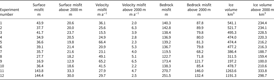
A value for all three misfits for all 12 experiments is also given for data above 2000 m since this is the area of most interest of this paper and where the model runs agree most. Calculated ice volume in km3 for the entire Renland Ice Cap based on the reconstructed ice thickness distribution for all the experiments. In all the model experiments PISM is forced with climate forcing data from RACMO2.3p2 from 1980 to 2014 and using ArcticDEM as surface topography.
The sensitivity of the reconstructed bed is investigated by performing experiments with different setting of the stress-balance model, basal till strength and ice rheology. Figure 4 shows the IceBridge data (subglacial topography and surface elevation) of the 2014 flight line in the west-east direction (blue line in Fig. 1, left) together with the altitude from the ArcticDEM for the same flight track. Furthermore, the topography cross section also show the modelled bedrock elevation from all the experiments after five iterations. The reconstructed beds clearly show that changes in basal parameters and stress model influence the estimation of the reconstructed subglacial topography of the ice cap. Overall the reconstructed bedrock topographies resemble the characteristic landscape of the area with deep valleys and a high-elevation plateau. With only the SIA approximation as the stress-balance model (as in experiments 11 and 12), the modelled bedrock along the edges of the ice cap and in the outlet glaciers is too low compared to observations and deep subglacial valleys form. This is due to the lack of sliding and high basal shear stress in the SIA approximation solution by the PISM model. With the SIA+SSA hybrid solution the modelled bedrock depends on the prescribed properties of the bedrock till. A soft bed with a low uniform till angle (as e.g. in experiment 9) leads to a too shallow reconstructed ice cap, while a more moderate uniform till angle (as in experiments 7 and 8) or a height dependent till angle (as in experiment 4) resemble the observed bedrock within 200 m along the IceBridge radar line (Fig. 4). The bedrock of the Renland Ice Cap is very complex, with mountains up to 300 m high within a few kilometres, which the model cannot resolve due to its resolution and the flow approximation. In addition, uncertainties in the assumed climate forcing and surface topography data can result in errors in the inferred bed topography. In particular, relatively small uncertainties in the assumed surface topography data can result in large errors in the inferred bed topography. See discussion below.
Cross section of IceBridge surface and subglacial elevation, ArcticDEM and reconstructed bed (after five iterations) from different till angle friction (ϕ), enhancement factor (E) and stress-balance model experiments in PISM along the CReSIS airborne radar track from 2014 (see Fig. 1, left) in the west-east direction. Similar plots can be made for the other radar tracks. Note all experiments are forced with the same constant climate forcing from RACMO2.3p2 and run to a steady state geometry.

We use the known bed height data from the airborne radar measurements from IceBridge to validate the reconstructed bedrocks. This is done by calculating the deviation between the modelled bed topographies and the three radar lines from 1998, 2014 and 2015 (see Fig. 1, left). The bedrock deviation is evaluated for all 12 experiments in PISM. A RMS bedrock misfit value between the radar lines and the model experiments after five iterations are shown in Table 2. These data will be used to define the best basal parameters when modelling the Renland Ice Cap.
The standard deviation of the modelled surface topography, ice thickness and surface velocity for results of iteration number 5 for all 12 experiments are shown in Figure 5. Both the modelled ice thickness and modelled surface topography plots show a best agreement for the inner parts of the two dome areas of the Renland Ice Cap, and the largest disagreements for the outlet glaciers, the area upstream of the largest outlet glaciers and around the ice-cap marginal zone. The std dev. of surface velocity shows the same pattern, where there is best agreement between the results for the inner parts of the ice cap and largest disagreements of the outlet glaciers. This shows that it is complicated to model a complex small ice cap with outlet glaciers, where the ice flow regimes of the interior ice cap and the outlet glaciers are significantly different depending on the amount of basal sliding.
Standard deviation of all 12 experiment after n = 5 iterations. (a) shows the ice thickness, (b) shows the surface topography, while (c) shows the surface velocity. The contours are the surface topography with 500 m intervals for 0–2000 m height and 100 m contour intervals above 2000 m.

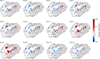
We use the known surface topography from ArcticDEM and surface velocities from Sentinel-1 to validate our model experiments with different stress-balance model and basal conditions, by calculating the misfits between the model and the observed data. Figure 6 shows the surface height misfit of the reconstructed surface topography after n = 5 iterations and the observed topography from ArcticDEM, while Figure 7 shows the surface velocity misfit of the reconstructed velocity and the Sentinel-1 velocity data after five iterations for all 12 experiments.
Surface height misfit of the reconstructed surface topography after n = 5 iterations and the ArcticDEM. All experiments where forced with the same climate forcing. The contours delineate 500 m surface elevation intervals from the DEM. The 12 different experiments use different values of till frictions angle (ϕ), enhancement factor (E) and stress-balance model (see Table 1).

Surface velocity misfit of the reconstructed velocity after n = 5 iterations and the Sentinel-1 velocity data. All experiments where forced with the same climate forcing. The contours delineate 500 m surface elevation intervals from the DEM. The 12 different experiments use different values of till frictions angle (ϕ), enhancement factor (E) and stress-balance model (see Table 1).

The surface height misfit plots show that the areas with the largest discrepancies are areas that are upstream of the outlet glaciers on the western dome of the ice cap, the three largest outlet glaciers and around the edge along the whole ice cap. From Figure 6 we can see a higher surface height misfit when only the SIA is used as stress-balance model and an overall lower surface height misfit when the material till strength ϕ is constant and lowest. A total surface height misfit value for all 12 experiments is given in Table 2. The surface velocity misfit plots show that the areas with the largest discrepancies of surface velocity are near the margins close to outlet glaciers or ice falls and in the same locations as where the highest std dev. of ice thickness are observed (Fig. 5). In the central part of the ice cap modelled velocity patterns are similar to observed velocities from satellites. Figure 7 shows a smaller velocity misfit in a few outlet glaciers when the SIA is used as stress-balance model compared to a larger misfit when the material till strength is at a lower constant value instead of having values ranging as a function of bed elevation (Eqn (4)). The opposite applies to the surface height misfit plots. A total surface velocity misfit value for all 12 experiments is given in Table 2, and shows that for both the entire ice cap and the area above 2000 m, the velocity misfits of the SIA experiments are in the middle. The performance of the surface velocity in the SIA experiments cannot be assessed without taking into account the surface elevation misfit, which is controlling the iterative inverse method.
The sensitivity of the reconstructed bed to changes in the material till strength is investigated by performing runs with different values for the material till strength ϕ (Eqn (4)) with values ranging either as a function of bed elevation between 5 and 40° or as a constant value between 10 and 30° (see Table 1). The material till strength affects the amount of basal lubrication, which influence the ice thickness distribution. These experiments were done in order to infer the complex subglacial topography, and at the same time match the modelled surface velocity to observations both in the slow-moving interior part of the ice cap and in the faster moving outlet glaciers. Our study shows that for models with a height dependent basal till friction angle, the reconstructed ice thickness is similar in the upper part of the outlet glaciers, with only small variations in the ice thickness between the different models. For models with a uniform till friction angle, the thickness distribution is influenced by the assumed till friction angle, both in the interior part of the ice cap and in the outlet glaciers. Similarly, the modelled surface velocities in the outlet glaciers exhibit a larger spread of over 100 m a−1 between the models assuming a uniform till friction angle, ϕ, while the spread between the models assuming a height dependent till friction angle is smaller. The surface height misfit as a function of number of the iterations is lower and more constant when using a constant value of till friction compared to values generated as a function of bed elevation, where the surface misfit is more than double for the first iterations (see Fig. 3). However, if we look at the modelled surface velocities compared to the observed velocity, a bed-height dependent till friction formulation captures the surface velocities at the upper part of main outlet glaciers much better than when the till friction is kept constant, especially if the constant till friction value gets to low (see Fig. 7).
We calculate the total ice volume from the reconstructed ice thickness for all experiments. Table 2 presents the calculated ice volume. The total ice volume in km3 of the Renland Ice Cap, based on the reconstructed ice thickness distribution, are calculated both for the entire ice cap and for the ice cap areas above 2000 m, which is the area where the model experiments agree most. The areas above 2000 m cover the central part of the two domes and none of the outlet glaciers are included. For all the experiments, the total ice volume for the entire ice cap varies between 200 and 1260 km3, a factor of 6.4 between the lowest and highest ice volume for the Renland Ice Cap, while a volume factor of 3.3 is found for the areas above 2000 m. In addition to the inverse iterative method, we also estimate the ice volume using a simple method based on the perfect plasticity assumption, where the bedrock topography is derived from modelled ice thickness (Machguth and others, Reference Machguth2013) and the ArcticDEM, we get a volume estimate of 365 km3. The ice thickness estimate, using this method, is only based on the surface slope, and assumes that the basal shear is uniform and constant over the entire ice cap.
To determine the best basal parameters, and thereby the best model experiment, for the Renland Ice Cap, we evaluate all the experiments by giving them a score based on the misfits of surface topography, surface velocity and bedrock topography along the radar lines. Each experiment is given a score based on each of the six misfit-columns in Table 2 and an average of these scores are calculated to provide the total score (see Table 3). The single best experiment with the best overall score after five iterations is experiment number 7, where the stress-balance model is a hybrid between the two shallow approximations, has an enhancement factor of 1, and a constant material till strength value. The ice thickness for experiment 7 is presented in Figure 8a. The data points in the circles are the ice thickness radar data from IceBridge. Comparing the observed ice thickness with the modelled ice thickness shows the biggest difference in the areas upstream of the three largest outlet glaciers. The reconstructed bedrock topography for experiment 7 with the best basal model parameters is shown in Figure 8b. It shows a landscape characterised by a high elevation plateau with steep slopes similar to the ice-free areas outside the ice cap.
A score for each experiment based on the misfits of surface topography, surface velocity and radar lines bedrock topography for the whole ice cap and area above 2000 m altitude
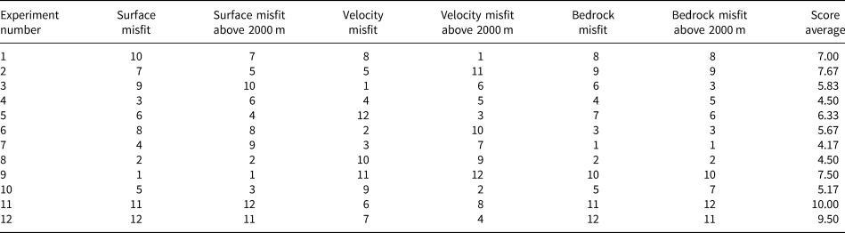
The overall best scores is calculated as the average of these scores.
(a) Simulated ice thickness and (b) the reconstructed bedrock elevation for experiment 7 after n = 5 iterations, while the data points in the circles are the radar data from the IceBridge (only every 90th radar point are plotted). The contours are the surface topography with 500 m intervals for 0–2000 m height and 100 m contour intervals above 2000 m.

We follow the approach by the Ice Thickness Models Intercomparison eXperiment (ITMIX) and combine various reconstruction approaches into our best estimate of ice volume. Here we calculate the average of the perfectly plastic result and the best three results from the 12 experiments to determine our best estimate of ice volume, and we find a total ice volume of 384 km3 of the Renland Ice Cap or 1 mm sea-level equivalent. The PISM results used to find the best ice volume are all based on ice flow with a SIA+SSA hybrid stress balance, but include both results with constant material till strength values and a result where the till strength value depends on bed elevation.
5. Discussion
Several studies have estimated global glacier volume from ice thickness distribution from surface characteristics (such as elevation and slope). In Table 4 we compare our result with the simple method, based on perfectly plastic assumption (Machguth and others, Reference Machguth2013), and two studies (Grinsted, Reference Grinsted2013; Farinotti and others, Reference Farinotti2019), both based on inferring the spatial ice thickness distribution from surface characteristics, an estimate of the glacier mass turnover and principles of ice flow. In our study, the results are also based on surface characteristics, but we improve the validating of the model results by additional information of the ice surface velocity and bed height. We note that our best estimate as well as the estimate based on the perfectly plastic method provide a lower ice volume than the two other studies. Our best estimate is calibrated against local and regional measurements from Greenland, which is not the case for the other methods. We use a more complex model that includes fast flowing outlet glaciers and adapted to the local conditions, while the two other studies are aiming at estimating the global glacier volume, and are using more general methods (Grinsted, Reference Grinsted2013; Farinotti and others, Reference Farinotti2019). Hence, we have more confidence in the estimated volume for the Renland Ice Cap presented in this study.
Overview of total ice volume for the Renland Ice Cap from different studies

The Grinsted (Reference Grinsted2013) estimate is updated using glacier outlines from World Glacier Inventory (WGI) (WGMS, 2012). aThis is our best estimate and determined as the average of the perfectly plastic estimate and the three best results from the inverse, iterative method.
The Renland Ice Cap is located at a 2 km high elevation plateau surrounded by steep slopes. Our inferred bedrock topography shows that deep valleys are incised into the bedrock underneath the ice cap on both sides of the Renland plateau. Figure 8b, where the radar data are plotted on top of the model data, shows that using the method from van Pelt and others (Reference van Pelt2013) for the Renland Ice Cap, the valleys at the bedrock cannot be reconstructed in the inner part of the ice cap where the observed surface topography is smooth. Overall, the bedrock topography is characterised by steep scarps and high plateaus, similar to the ice free landscape surrounding the Renland Ice Cap in East Greenland, and the method seems to successfully capture these landscape characteristics underneath the ice cap. However, we find that the detailed features of the inferred ice thickness are sensitive to the assumed basal conditions in the ice flow model in addition to the errors induced by the uncertainty in the input datasets. The amount of basal sliding severely affect the ice flux, and the modelled ice thickness are particularly sensitive to the basal conditions near the margin and upstream from the outlet glaciers, that drain the central part of the ice cap located at a high plateau through steep and deep valleys down to sea level. In these specific locations with particular complex ice flow, the ice thickness differs by up to several hundred metres among our model runs depending on the choice of model parameters, although the model thickness agree within ~50 m in the interior parts of the ice cap.
The difficulties in reconstructing ice thickness in areas with complex flow has been pointed out by previous studies. Results from 17 different models in ITMIX showed that ice thickness estimates can differ considerably when inferring ice thickness from characteristics of the surface (Farinotti and others, Reference Farinotti2017). Farinotti and others (Reference Farinotti2017) concluded that techniques to deduce the ice thickness distribution without direct field measurements can give good overall results, but they are insufficient when applying complex modelling methods to resolve bedrock features at high spatial resolution. In our study, we find that the ice thickness estimates are sensitive to the choice of model settings related to basal sliding in areas with complex flow. The Renland Ice Cap with its very complex bedrock topography represents a very challenging case, because the limited spatial resolution and incomplete physics of the ice flow model smooth out features in the flow and the modelled surface topography. In addition, the bedrock under the central part of the ice cap has several deep troughs/valleys, and radar and ice core records suggest that part of the deep ice in a valley underneath the central part of the ice cap is stagnant (Taranczewski and others, Reference Taranczewski2019), which will mask out bedrock features in the smooth surface topography. In general the bed to surface transfer in relatively flat terrain is small, meaning that bed undulations show only weak surface expressions (Raymond and Gudmundsson, Reference Raymond and Gudmundsson2005). This means that a very detailed DEM is needed for the Renland Ice Cap, presumably more detailed than the ArcticDEM used here. With such a detailed DEM it could be that the surface (and bed) misfit would have continued to drop for more than five iterations, implying that also smaller scale features in the bed are recovered. As shown in van Pelt and others (Reference van Pelt2013) large-scale bed undulations are recovered earlier, i.e. after less iterations, than smaller-scale patterns. In the study by van Pelt and others (Reference van Pelt2013), applying the same ice flow model and the same technique, the method gave results closer to observed data when applied to a glacier in Svalbard with more simple geometry. Experience from our study here suggests that the most significant reasons for this better agreement are (1) a better DEM exists for Svalbard (Nordenskildbreen) than the Renland Ice Cap, (2) the Renland Ice Cap has a large ice low-sloping ice plateau, which is challenging for the inverse routine and (3) that the dynamics of Renland Ice Cap are more difficult to model, in particular thermodynamics and sliding. As mentioned earlier, the inverse approach used here (van Pelt and others, Reference van Pelt2013) has performed well in comparison with other thickness inversion methods in the ITMIX intercomparison experiment (Farinotti and others, Reference Farinotti2017), and is also used in a second phase of ITMIX, again confirming the good performance of the approach (Farinotti and others, Reference Farinotti2021).
Our reconstructed basal topography results show that the model parameters controlling the ice softness and basal sliding, i.e. ice softness, lubrication, basal material till strength, are important and influence both the modelled surface velocity values and the estimated ice thickness distribution, and thereby the calculated total ice volume, and in this way the maximum potential contribution to sea-level rise in a warming climate from the ice cap. We ran the model with and without basal sliding (i.e. SIA runs), and found that SIA modelling alone cannot match the observed ice thickness and surface velocities. The basal sliding affects how the basal topography is transmitted to the surface topography. This can lead to strong non-linear effects in the velocity field when the bedrock is updated, e.g. a small change in the bedrock topography can ‘turn-on’ an ice stream and lead to a lowering of the surface topography. We observed in several runs that additional iterations could lead to turning on and off of fast flowing ice in a localised area upstream of the Apusinikajik Glacier (Fig. 1), perhaps due to the complex drainage pattern with several glaciers draining into the Apusinikajik Glacier. Small changes in the ice thickness between the iterations can affect the drainage pattern, resulting in large localised changes in surface velocity. However, all models agree in the interior parts of the ice cap, despite a great variation between the model parameters in the different runs. For the total ice thickness, the variations between the best models in the area above 2000 m are ~15%.
The results of the iterative inverse method of estimating the ice thickness and bedrock topography are not only dependent on the choice of model parameters in the ice flow model, but also on uncertainties in the observed surface topography and the assumed climate forcing (SMB and ice temperature). Uncertainties in the surface topography and in the assumed SMB, affecting the ice flux when the model is run to steady state, can propagate into the inferred bedrock. The success of the inverse method to infer the bedrock topography depends on the accuracy of the input data as well as the physics of the ice flow model, and our study shows that while both these factors are important, the uncertainties in basal sliding parameters and ice softness can lead to particular large errors in the estimated ice volume for the Renland Ice Cap. However, we find the best matching ice thickness when the velocities are not matching well, see Table 3, suggesting that there may be biases in the SMB forcing, which controls the mass fluxes from high to low elevations. For other glaciers, the uncertainties in input datasets, e.g. either the surface topography or the atmospheric climate forcing, may be more significant than the choice of basal model parameters.
van Pelt and others (Reference van Pelt2013) showed that the inverse ice thickness estimation routine works best with a time-dependent climate forcing, ideally covering a period as long as the response time of the glacier or ice cap. In our study, a 35-year climate forcing from RACMO2.3 is averaged to generate a time-independent forcing that is used to generate steady-state geometries at the end of every iterative model simulation. From the Renland ice core records, it is believed that the Renland Ice Cap has remained relatively stable over the last glacial cycle (Johnsen and others, Reference Johnsen1992). Our modelling shows that the Renland Ice Cap builds up from no ice and is in steady state after 500–2000 years. During the last 500–2000 years, the climate records from Greenland ice cores show a relatively stable climate, and the Holocene climatic optimum was ~8–5 ka ago in Greenland (Nielsen and others, Reference Nielsen, Adalgeirsdóttir, Gkinis, Nuterman and Hvidberg2018). Therefore, we believe that the uncertainty due to using a constant climate forcing is minor for the Renland Ice Cap. However, the few outlet glaciers that reach to lower altitudes may respond more quickly to climate changes, and their extent may not be accurately reproduced by the method.
6. Conclusions
In this study, we use an inverse approach to infer the ice thickness distribution and the bedrock topography from characteristics of the surface of an ice cap, and further to estimate the total ice cap volume. We estimate the ice thickness and basal topography for the Renland Ice Cap by using an ice flow model, forced with climate data from a RCM and combined with an iterative inverse method, where the bedrock heights are adjusted in order to minimise the deviation between the modelled and observed surface topography. We investigate the sensitivity of the inferred bedrock to the ice physics and model parameters controlling the basal conditions using the iterative approach by van Pelt and others (Reference van Pelt2013) and we evaluate the results for the Renland Ice Cap on basis of surface topography data from ArcticDEM, radar depth sounder data from IceBridge and surface velocity from Sentinel-1 satellite. The effects of the stress-balance model, the ice rheology and bedrock parameters on the reconstructed bedrock and ice thickness distribution are investigated. We discuss the sensitivity of the surface height misfit, ice surface velocity and misfit of bedrock to model parameters, where radar information is available. With this method, we are able to reconstruct the overall pattern of ice thickness and bedrock elevation beneath the Renland Ice Cap. Our inferred bedrock topography shows a landscape characterised by steep slopes and high elevation plateaus, similar to the ice free landscape surrounding the Renland peninsula. However, upstream from the deep outlet glaciers in areas with complex flow, we cannot confidently reconstruct the detailed features of the bedrock.
In the study, we found that the inferred bedrock topography for the Renland Ice Cap in areas of complex flow is sensitive to the choice of model parameters controlling the basal conditions. Hence, optimum basal parameters could be selected by reducing the misfit between the model output and observations of surface height, bed height and ice velocity. Still, recovering small-scale features in the bed appeared difficult, which can be primarily ascribed to uncertainties in the input data (surface height and climate forcing) and model physics. Our results show deviations in ice thickness among the experiments of up to several hundred metres in particular areas upstream from outlet glaciers, but all models agree within 50 m in the interior parts of the ice caps. The resulting estimated ice volume in these interior areas vary with 10% between the best experiments. By evaluating our results against measured airborne radar measurement and satellite observed surface velocity, we found that the best model experiment had an enhancement factor of 1 and uniform basal sliding parameters. Resulting in a total ice volume of 386 km3 of the Renland Ice Cap. A best estimate with a total ice volume of 384 km3 of the Renland Ice Cap is found by combining four different results, including a perfectly plastic estimate, and the three best results from the iterative inverse method (assuming SIA+SSA constant material till strength values or SIA+SSA bed elevation dependent material till strength value), as inspired by the average ITMIX consensus estimate (Farinotti and others, Reference Farinotti2017).
As peripheral glaciers and ice caps are predominately land terminating and thus insensitive to marine processes, they provide a more direct measure of glacier sensitivity to atmospheric climate variability. The inverse method is therefore a good approach to modelling land terminating glaciers and ice caps, since the model only use atmospheric forcing as input, while for marine terminating glaciers ocean forcing would also be needed. The surface topography is an important parameter for the method as well, since only those bedrock variations that are reflected in the surface topography can be reconstructed. Undulations in surface topography can thus be indicative of valleys and mountains beneath the ice, and thereby contribute to estimate how sensitive the glacier is to climate change.
For many glaciers and ice caps, bedrock data are scarce or absent and the approach used in this study provides a reasonable method for spin-up for experiments with ice flow models, in addition to reconstructing the basal topography. Knowing the geometry of the bedrock and ice thickness distribution of the Renland Ice Cap is a first step to investigate the evolution of the ice cap in the past. Addressing these questions provides an insight into how the ice cap may respond in the future and help to understand if the ice cap over longer time scales has contributed to sea-level change.
Acknowledgements
The RECAP ice coring effort was financed by the Danish Research Council through a Sapere Aude grant, the NSF through the Division of Polar Programs, the Alfred Wegener Institute and the European Research Council under the European Community's Seventh Framework Programme (FP7/2007–2013)/ERC grant agreement 610055 through the Ice2Ice project and the Early Human Impact project (267696). This study was supported by the Villum Investigator Project IceFlow (no. 16572). The authors acknowledge the development of PISM, which is supported by NASA grants NNX13AM16G and NNX13AK27G. We acknowledge the use of data and/or data products from CReSIS generated with support from the University of Kansas, NSF grant ANT-0424589, and NASA Operation IceBridge grant NNX16AH54G. The ice velocity map were produced from ESA Sentinel-1 remote-sensing data as part the Programme for Monitoring of the Greenland Ice Sheet (PROMICE) and were provided by Anne M. Solgaard from the Geological Survey of Denmark and Greenland (GEUS). We thanks NASA National Snow and Ice Data Center Distributed Active Archive Center for the MEaSURES Greenland Ice Mapping Project (GIMP) Digital Elevation Model, Version 1.5.3. We used ArcticDEM data, created from DigitalGlobe, Inc., imagery 2011–2016, and provided by the Polar Geospatial Center under NSF OPP awards 1043681, 1559691 and 1542736. We wish to acknowledge Brice Noël, Universiteit Utrecht, for producing and making available RACMO2.3p2 climate model output. Finally, we thank the anonymous reviewers for comments that helped improve this manuscript.
Author contributions
C.S. Hvidberg and I. Koldtoft designed the study. I. Koldtoft prepared the data and performed the model runs with input from C.S. Hvidberg and B.M. Vinther. I. Koldtoft created all figures and wrote a draft version of the paper. All authors edited and discussed the final manuscript.


 Open access