





1. Introduction
The Faraday effect provides a unique probe of the magneto-ionic medium of the universe. The Faraday rotation measure (RM) of a linearly polarised radio source is proportional to the product of the thermal electron density and the magnetic field parallel to and integrated along the line of sight. Through collecting large numbers of RMs across the sky from background sources, we can execute a ‘rotation measure grid’ experiment (Gaensler et al. Reference Gaensler, Beck and Feretti2004). These RM grids can then be used to illuminate foreground objects of interest such as the Milky Way (e.g. Dickey et al. Reference Dickey2022), nearby galaxies (e.g. Livingston et al. Reference Livingston2022, Reference Livingston2024; Stein et al. Reference Stein2025), groups and clusters (e.g. Anderson et al. Reference Anderson2021, Reference Anderson2024; Osinga et al. Reference Osinga2022), and even the cosmic web (e.g. Carretti et al. Reference Carretti2022, Reference Carretti2023, Reference Carretti2025). Using an external constraint on electron density, such as H $\alpha$
emission, it is possible to use RM grids to measure magnetic field strength and structure (see e.g. Harvey-Smith et al. Reference Harvey-Smith, Madsen and Gaensler2011). Conversely, the line-of-sight magnetic fields can act as a ‘dye tracer’, allowing RM grids to provide a uniquely sensitive probe of low-density thermal gas (Anderson et al. Reference Anderson2021, Reference Anderson2024).
$\alpha$
emission, it is possible to use RM grids to measure magnetic field strength and structure (see e.g. Harvey-Smith et al. Reference Harvey-Smith, Madsen and Gaensler2011). Conversely, the line-of-sight magnetic fields can act as a ‘dye tracer’, allowing RM grids to provide a uniquely sensitive probe of low-density thermal gas (Anderson et al. Reference Anderson2021, Reference Anderson2024).
The scientific yield of an RM grid is determined by four primary observational factors. First, we require radio continuum observations across a broad bandwidth. At its most simplistic, sampling many values of wavelength-squared ( $\lambda^2$
) circumvents ambiguities in the determined RM. Brentjens & de Bruyn (Reference Brentjens and de Bruyn2005) and Dickey et al. (Reference Dickey2019) further describe the impacts of channelization on the RM spread function (RMSF). Brentjens & de Bruyn (Reference Brentjens and de Bruyn2005) give the full-width at half-maximum (FWHM) Faraday depth resolution (
$\lambda^2$
) circumvents ambiguities in the determined RM. Brentjens & de Bruyn (Reference Brentjens and de Bruyn2005) and Dickey et al. (Reference Dickey2019) further describe the impacts of channelization on the RM spread function (RMSF). Brentjens & de Bruyn (Reference Brentjens and de Bruyn2005) give the full-width at half-maximum (FWHM) Faraday depth resolution ( $\delta\phi$
), the ‘maximum Faraday depth scale’ (
$\delta\phi$
), the ‘maximum Faraday depth scale’ ( $\phi_{\text{max-scale}}$
), and the maximum Faraday depth (
$\phi_{\text{max-scale}}$
), and the maximum Faraday depth ( $\phi_{\text{max}}$
) in their Equations (61), (62), and (63) respectively. We note that
$\phi_{\text{max}}$
) in their Equations (61), (62), and (63) respectively. We note that $\phi_{\text{max}}$
is inversely proportional to the nominal channel size in
$\phi_{\text{max}}$
is inversely proportional to the nominal channel size in $\lambda^2$
(
$\lambda^2$
( $\delta\lambda^2$
). Having sufficiently large
$\delta\lambda^2$
). Having sufficiently large $\phi_{\text{max-scale}}$
and with respect to
$\phi_{\text{max-scale}}$
and with respect to $\delta\phi$
allows the ‘Faraday complexity’ to be resolved in Farday depth (see e.g. Alger et al. Reference Alger2021). Second, we require a survey across a wide area of the sky. Wide areal coverage is needed to characterise large-scale foreground structure, such as the RM signature of the Milky Way. Third, we desire a survey with high sensitivity. The areal density of RMs across the sky determines the ‘resolution’ of our RM grid. Finally, we require high angular resolution. Such resolution is required to enable the study of the intrinsic individual sources, such as the lobes of radio galaxies (e.g. Anderson et al. Reference Anderson2018a,Reference Andersonb) or from the diffuse emission of the Milky Way (e.g. Landecker Reference Landecker2012; Erceg et al. Reference Erceg2024). As discussed in (Thomson et al. Reference Thomson2023, hereafter Paper Reference ThomsonIII), the historical compilation of RMs by Van Eck et al. (Reference Van Eck2023) is dominated by the catalogue from the NRAO VLA Sky Survey (Condon et al. Reference Condon1998; Taylor et al. Reference Taylor, Stil and Sunstrum2009, hereafter Reference Taylor, Stil and SunstrumNVSS). Reference Taylor, Stil and SunstrumNVSS was derived from two narrowly spaced frequencies at
$\delta\phi$
allows the ‘Faraday complexity’ to be resolved in Farday depth (see e.g. Alger et al. Reference Alger2021). Second, we require a survey across a wide area of the sky. Wide areal coverage is needed to characterise large-scale foreground structure, such as the RM signature of the Milky Way. Third, we desire a survey with high sensitivity. The areal density of RMs across the sky determines the ‘resolution’ of our RM grid. Finally, we require high angular resolution. Such resolution is required to enable the study of the intrinsic individual sources, such as the lobes of radio galaxies (e.g. Anderson et al. Reference Anderson2018a,Reference Andersonb) or from the diffuse emission of the Milky Way (e.g. Landecker Reference Landecker2012; Erceg et al. Reference Erceg2024). As discussed in (Thomson et al. Reference Thomson2023, hereafter Paper Reference ThomsonIII), the historical compilation of RMs by Van Eck et al. (Reference Van Eck2023) is dominated by the catalogue from the NRAO VLA Sky Survey (Condon et al. Reference Condon1998; Taylor et al. Reference Taylor, Stil and Sunstrum2009, hereafter Reference Taylor, Stil and SunstrumNVSS). Reference Taylor, Stil and SunstrumNVSS was derived from two narrowly spaced frequencies at $\sim\!{1.4}\,\mathrm{GHz}$
, and only provides an areal RM density of
$\sim\!{1.4}\,\mathrm{GHz}$
, and only provides an areal RM density of $\sim\!{1}\,\mathrm{deg^{-2}}$
. The Southern hemisphere is more sparsely sampled, with Schnitzeler et al. (Reference Schnitzeler2019), hereafter Reference SchnitzelerS-PASS/ATCA only providing an RM density of
$\sim\!{1}\,\mathrm{deg^{-2}}$
. The Southern hemisphere is more sparsely sampled, with Schnitzeler et al. (Reference Schnitzeler2019), hereafter Reference SchnitzelerS-PASS/ATCA only providing an RM density of $\sim\!{0.2}\mathrm{deg}^{-2}$
up to a declination of
$\sim\!{0.2}\mathrm{deg}^{-2}$
up to a declination of ${0}^{\circ}$
.
${0}^{\circ}$
.
As a purpose-built survey instrument, the Australian SKA Pathfinder radio telescope (ASKAP, Hotan et al. Reference Hotan2021) enables a generational leap in polarisation surveys. The primary polarisation Survey Science Project with ASKAP is Polarisation Sky Survey of the Universe’s Magnetism (POSSUM, Gaensler et al. Reference Gaensler2025). At the end of the 5-year survey campaigns POSSUM is expected to provide $\sim\!{7.75}\times10^5$
(
$\sim\!{7.75}\times10^5$
( $\sim\!{8.77}\times10^5$
) RMs covering
$\sim\!{8.77}\times10^5$
) RMs covering $2\pi\mathrm{sr}$
(
$2\pi\mathrm{sr}$
( $1.47\pi\,\mathrm{sr}$
) at 800–1 088 MHz (800–1 088 MHz + 1 296–1 440 MHz) (Vanderwoude et al. Reference Vanderwoude2024). We note that the low-frequency component of POSSUM is fully commensal with the Evolutionary Map of the Universe survey (EMU, Hopkins et al. Reference Hopkins2025).
$1.47\pi\,\mathrm{sr}$
) at 800–1 088 MHz (800–1 088 MHz + 1 296–1 440 MHz) (Vanderwoude et al. Reference Vanderwoude2024). We note that the low-frequency component of POSSUM is fully commensal with the Evolutionary Map of the Universe survey (EMU, Hopkins et al. Reference Hopkins2025).
The ASKAP Observatory has conducted the Rapid ASKAP Continuum Survey (RACS, McConnell et al. Reference McConnell2020, hereafter Paper Reference McConnellI) both in preparation for, and in support of, the full Survey Science Projects such as POSSUM. RACS is being conducted over multiple epochs and covers the full frequency range available to ASKAP. To date 5 epochs of RACS have been observed, namely; RACS-low1 (Paper Reference McConnellI) and low2 at 887.5 MHz, low3 at 943.5 MHz (this work, and Galvin et al. in prep), mid at 1 367.5 MHz (Duchesne et al. Reference Duchesne2023, hereafter Paper Reference DuchesneIV), and high at 1 655.5 MHz (Duchesne et al. Reference Duchesne2025, hereafter Paper Reference DuchesneVI). Catalogues in total intensity were presented by Hale et al. (Reference Hale2021, hereafter Paper Reference HaleII) for RACS-low1, Duchesne et al. (Reference Duchesne2024, hereafter Paper Reference DuchesneV) for RACS-mid, and Paper Reference DuchesneVI for RACS-high.
In Paper Reference ThomsonIII we described the first data release (DR1) of Spectra and Polarisation in Cutouts of Extragalactic sources from RACS (SPICE-RACS). SPICE-RACS is a joint project between the ASKAP Observatory and the POSSUM Collaboration. Its aim is to derive linear polarisation results from RACS using spatial cutouts around sources detected in total intensity. The DR1 catalogue was derived from 30 RACS-low1 fields with a sensitivity of $\sim\!{150}\,\unicode{x03BC}\mathrm{Jy}/\mathrm{PSF}$
in linear polarisation (Thomson et al. Reference Thomson2024). The catalogue provided detections of 5 818 linearly polarised components over
$\sim\!{150}\,\unicode{x03BC}\mathrm{Jy}/\mathrm{PSF}$
in linear polarisation (Thomson et al. Reference Thomson2024). The catalogue provided detections of 5 818 linearly polarised components over $\sim\!{1}\,300\,\mathrm{deg}^{-2}$
; an areal RM density of
$\sim\!{1}\,300\,\mathrm{deg}^{-2}$
; an areal RM density of $\sim\!{4.5}\,\mathrm{deg}^{-2}$
.
$\sim\!{4.5}\,\mathrm{deg}^{-2}$
.
In this paper, we introduce the second SPICE-RACS data release (DR2), which covers the entire Southern sky visible to ASKAP; a total area of $3.5\pi\,\mathrm{sr}$
. This paper is structured as follows. In Section 2, we describe the observations and data used in this data release. In Section 3, we explain our data processing and pipeline. Next, in Section 4, we provide an overview of the catalogues included in this paper. We then present a brief analysis of the data in Section 5, and set out our conclusions in Section 6.
$3.5\pi\,\mathrm{sr}$
. This paper is structured as follows. In Section 2, we describe the observations and data used in this data release. In Section 3, we explain our data processing and pipeline. Next, in Section 4, we provide an overview of the catalogues included in this paper. We then present a brief analysis of the data in Section 5, and set out our conclusions in Section 6.
2. Data
For this second data release we elect to use the third epoch of the low-band RACS (RACS-low3) as it provides a number of improvements over previous epochs. RACS-low3 uses a central frequency of 943.5 MHz (matching the central frequency of EMU/POSSUM), which in turn yields a lower system temperature (Hotan et al. Reference Hotan2021). Unlike RACS-low1 and low2, RACS-low3 was observed with a closepack_36 footprint, with a sky tiling exactly matching RACS-mid and RACS-high (see Paper Reference DuchesneIV), as well as the EMU/POSSUM survey. We show the footprint of the RACS-low3 beams in Figure 1. The ASKAP Observatory conducted an initial observing run of RACS-low3 from December 2023 to February 2024, with an additional set of re-observations completed from May to April 2024. The re-observations were requested to help improve a small subset of data that had reduced data quality and high levels of flagging. Here we will use the initial set of observations, and leave the inclusion of the later re-observations to a future data release.
The field of view of RACS-low3 as measured by holography. We show the 50% level of the Stokes I response beams at 800 MHz and 1088 MHz in solid and dashed contours, respectively. We show the beam positions with respect to the telescope pointing centre, and colour each beam by its respective number.

The initial observing campaign for RACS-low3 consisted of 1 615 target observations of 1 493 unique fields. Each observation is uniquely identified by a ‘scheduling block identifier’ (SBID), with each field having its own unique name derived from its central coordinates. RACS-low3 was observed under a single set of ‘parent’ beamforming weightsFootnote a (with SBID 55217), meaning that the formed beams should be common amongst all observations. The ASKAP Observatory conducted holography of the RACS-low3 beams at the start and end of the observing run with SBIDs 55219 and 59276, respectively. Throughout this entire work we use the holography from SBID 55219 for self-consistency.
Each individual RACS-low3 observation was processed autonomously by the ASKAP Observatory pipeline (Guzman et al. Reference Guzman2019). This processing included flagging, primary bandpass calibration, and total intensity imaging with self-calibration. For further details on this processing pipeline, we refer the reader to Paper Reference McConnellI. The resulting total intensity images cover the entire Southern sky up to $\delta\sim + {49}^{\circ}$
with a median interquartile range (IQR)Footnote
b
rms noise of
$\delta\sim + {49}^{\circ}$
with a median interquartile range (IQR)Footnote
b
rms noise of $190 \substack{+60\\-32}\,\mathrm{\mu{Jy}/ PSF}$
. The calibrated visibilities, mosaicked images, and initial source lists for each field were deposited and released on the CSIRO ASKAP Data Archive (CASDA, Huynh et al. Reference Huynh, Dempsey, Whiting, Ophel, Ballester, Ibsen, Solar and Shortridge2020).
$190 \substack{+60\\-32}\,\mathrm{\mu{Jy}/ PSF}$
. The calibrated visibilities, mosaicked images, and initial source lists for each field were deposited and released on the CSIRO ASKAP Data Archive (CASDA, Huynh et al. Reference Huynh, Dempsey, Whiting, Ophel, Ballester, Ibsen, Solar and Shortridge2020).
For this data release, we will present the polarisation results from processing each individual RACS-low3 field independently. Whilst the edges of each field will lack the maximum possible sensitivity, the time-domain information will be retained. This data release will therefore be similar to the ‘time domain’ catalogue from Paper Reference DuchesneV. We will publish a ‘full sensitivity’ catalogue in a future data release.
3. Processing
3.1 Initial cataloguing
For the purpose of guiding polarised source extraction, we make use of a total intensity source catalogue constructed from the Observatory-processed RACS-low3 Stokes I images. The construction of the Stokes I catalogue follows processes used for previous RACS epochs (Paper Reference HaleII; Paper Reference DuchesneV; Paper Reference DuchesneVI) and makes use of the overlapping images to form full-sensitivity mosaics for each unique RACS-low3 field. Unlike our polarisation catalogue, this total intensity source-finding catalogue is de-duplicated.
The PSF of the RACS-low3 observations varies significantly over the survey region, largely as a function of declination, with a major axis FWHM ranging from $\sim\!{12}\,\mathrm{to}\,{60}$
arcsec. To account for this variation, we follow Paper Reference DuchesneV and use the lowest common resolution from all overlapping images that make up each mosaic rather than a fixed angular resolution over the whole survey. We use beamcon_2D from RACS-toolsFootnote
c
to find and convolve to the smallest fitting PSF. Once the individual images are convolved for each mosaic, we use SWarp (Bertin et al. Reference Bertin, Bohlender, Durand and Handley2002) for regridding and co-addition, weighting individual images by the output weight files from the ASKAPsoft processing. These weights are a combination of the primary beam attenuation and the number of unflagged visibilities for a given PAF beam dataset.
$\sim\!{12}\,\mathrm{to}\,{60}$
arcsec. To account for this variation, we follow Paper Reference DuchesneV and use the lowest common resolution from all overlapping images that make up each mosaic rather than a fixed angular resolution over the whole survey. We use beamcon_2D from RACS-toolsFootnote
c
to find and convolve to the smallest fitting PSF. Once the individual images are convolved for each mosaic, we use SWarp (Bertin et al. Reference Bertin, Bohlender, Durand and Handley2002) for regridding and co-addition, weighting individual images by the output weight files from the ASKAPsoft processing. These weights are a combination of the primary beam attenuation and the number of unflagged visibilities for a given PAF beam dataset.
Following Paper Reference DuchesneV, we use PyBDSF Footnote d (Mohan & Rafferty Reference Mohan and Rafferty2015) for source-finding and characterisation. The source lists for each mosaic are then merged, with duplicate measurements of sources in overlapping regions removed to retain only a single measurement for each source. PyBDSF produces a list of 2D Gaussian components alongside each source list. We have found previously that sources can be modelled with more Gaussian components than necessary (Paper Reference DuchesneV), so for sources that have a ratio of integrated to peak flux density less than the median for a given mosaic source list, we assume these are true point sources and regroup their components (if more than one component) into a single component. This is done by summing the flux density and taking the size as reported in the corresponding source list. The position is also taken from the source list rather than an average from the component list. Source lists for each mosaic are then merged together, with duplicate measurements in overlapping regions removed following Paper Reference DuchesneV. The contiguous, de-duplicated catalogues contain 3 980 923 sources and 5 479 676 Gaussian components.
3.2 Arrakis
In Paper Reference ThomsonIII we presented our highly parallelised processing pipeline, Arrakis,Footnote e which was used to derive the DR1 catalogue. Arrakis is built in Python using the Prefect and Dask (Dask Development Team 2016) frameworks; allowing it to be run and scaled on a huge number of hardware platforms. Version 1 (v1) of Arrakis was a post-processing pipeline which required us to use portions of the RACS and ASKAP pipelines to produce images for polarisation analysis. Here we present v2 of Arrakis, which is a fully self-contained pipeline that can take calibrated ASKAP visibilities, such as those available on CASDA, and produce polarisation images and catalogues ready for scientific use. Here we will provide a description of the new, or substantially modified, components of Arrakis. Unless otherwise described, the primary functions of Arrakis remains the same as in Paper Reference ThomsonIII. All of our Arrakis processing was run on the CSIRO High Performance Computing cluster Petrichor.
3.2.1 Spectro-polarimetric imaging
In producing images for polarisation analysis from ASKAP we have two primary requirements. First, we require suitable handling of the non-co-planar effects (i.e. the ‘w-term’, Cornwell et al. Reference Cornwell, Golap and Bhatnagar2008) when producing wide-field images. Second, and perhaps most critically, we require multiple output channel images in order to perform rotation measure synthesis (RM-synthesis, Brentjens & de Bruyn Reference Brentjens and de Bruyn2005). With these requirements in mind, we chose to use the WSClean imager (Offringa et al. Reference Offringa2014; Offringa & Smirnov Reference Offringa and Smirnov2017). The wgridder algorithm (Arras et al. Reference Arras2021; Ye et al. Reference Ye, Gull, Tan and Nikolic2022) in WSClean provides highly efficient handling of the w-term, and is parallelisable across multiple channels images when gridding and de-gridding visibilities. Further, when producing a frequency cube across multiple Stokes parameters the options join-channels, join-polarizations, and squared-channel-joining options enable WSClean to clean the narrow channels utilising the information from the full bandwidth and polarisations. This provides improved image quality in comparison to the Taylor-term imaging or per-channel imaging performed by the YandaSoft cimager/imager (Guzman et al. Reference Guzman2019) used for SPICE-RACS DR1. In Arrakis v2 we have implemented a thin Python wrapper for WSClean which is called within the arrakis.imager pipeflow flow.
Visibilities produced and calibrated by the ASKAPsoft pipeline are not directly compatible with imagers like WSClean. First, the reported fields of each of the 36 beams are reported as the centre of the field, which is not the same as the pointing centre or phase centre of any of the individual beams. A common field centre would be needed in the case of joint-beam deconvolution, however we chose to image each beam independently. Furthermore, the correlations stored in Observatory-processed visibilities are initially in the instrumental frame. ASKAP has a unique ‘roll’ axis which allows the feeds to be rotated arbitrarily with respect to the sky and as a function of time. In practice, however, the roll axis is driven such that ASKAP operates as an equatorial telescope, with a constant rotational offset from the celestial coordinate frame. Finally, ASKAPsoft adopts a Stokes definition in which $I = XX + YY$
. WSClean, however, assumes that the input data is in the IAU polarisation standard, where X and Y align with celestial North and East respectively. WSClean also adopts the Stokes convention that
$I = XX + YY$
. WSClean, however, assumes that the input data is in the IAU polarisation standard, where X and Y align with celestial North and East respectively. WSClean also adopts the Stokes convention that $I = (XX + YY) / 2$
. We have implemented a Python library FixMS
Footnote
f
which can convert ASKAPsoft visibilities into a format compatible with WSClean. We detail the formalism of this conversion in Appendix B. For SPICE-RACS DR2 we use version v0.2.9 of FixMS.
$I = (XX + YY) / 2$
. We have implemented a Python library FixMS
Footnote
f
which can convert ASKAPsoft visibilities into a format compatible with WSClean. We detail the formalism of this conversion in Appendix B. For SPICE-RACS DR2 we use version v0.2.9 of FixMS.
We make use of a common set of WSClean options, with some direction-dependent settings. For all images we enable the wgridder and join-channels options. We image Stokes I independently, and Stokes Q and U jointly with join-polarizations and squared-channel-joining. By default we use an image size of 6 144 pixels, with a cell size of ${2.5}^{\prime\prime}$
, and a visibility weighting of Briggs robust
${2.5}^{\prime\prime}$
, and a visibility weighting of Briggs robust $-0.5$
(Briggs Reference Briggs1995). We apply a cut in uv-space of 200 wavelengths to suppress any short-baseline interference (such as the Sun). In the case of clean divergence, usually caused by a bright source outside the image boundary, we manually increased the image size to encompass the source. We use clean major cycles with a mgain of 0.6. Since our focus for SPICE-RACS is primarily on characterisation of compact components, and we are using a uv-cut, we do not enable multiscale cleaning.
$-0.5$
(Briggs Reference Briggs1995). We apply a cut in uv-space of 200 wavelengths to suppress any short-baseline interference (such as the Sun). In the case of clean divergence, usually caused by a bright source outside the image boundary, we manually increased the image size to encompass the source. We use clean major cycles with a mgain of 0.6. Since our focus for SPICE-RACS is primarily on characterisation of compact components, and we are using a uv-cut, we do not enable multiscale cleaning.
To derive the polarisation properties of our components we use RM-synthesis Brentjens & de Bruyn (Reference Brentjens and de Bruyn2005), which produces a Faraday depth ( $\phi$
) dispersion function (FDF) via a Fourier transform. The Faraday depth defines the amount of Faraday rotation integrated along the line of sight. In the most simplistic case the Faraday depth reduces to the RM. Here we will report the Faraday depth at the peak in the FDF as an RM.
$\phi$
) dispersion function (FDF) via a Fourier transform. The Faraday depth defines the amount of Faraday rotation integrated along the line of sight. In the most simplistic case the Faraday depth reduces to the RM. Here we will report the Faraday depth at the peak in the FDF as an RM.
Here we use the software package RM-tools (Purcell et al. Reference Purcell, Van Eck, West, Sun and Gaensler2020, Van Eck in prep.) to compute Faraday depth information. RM-tools takes $\delta\lambda^2$
to be the largest channel in
$\delta\lambda^2$
to be the largest channel in $\lambda^2$
. We set the number of channels for a given field based on its central Galactic latitude. If a field centre has Galactic latitude
$\lambda^2$
. We set the number of channels for a given field based on its central Galactic latitude. If a field centre has Galactic latitude $|b|\gt{10}^{\circ}$
we produce 36 channel images, otherwise we produce 72. These channellisations provide maximum Faraday depths of
$|b|\gt{10}^{\circ}$
we produce 36 channel images, otherwise we produce 72. These channellisations provide maximum Faraday depths of $\sim\!{630}\,\mathrm{rad\,m}^{-2}$
and
$\sim\!{630}\,\mathrm{rad\,m}^{-2}$
and $\sim\!{1}\,250\,\mathrm{rad\,m}^{-2}$
, respectively. This allows us to remain sensitive to the higher magnitude RMs we expect towards the Galactic plane. We summarise these values, and the other properties of the RMSF, in Table 1.
$\sim\!{1}\,250\,\mathrm{rad\,m}^{-2}$
, respectively. This allows us to remain sensitive to the higher magnitude RMs we expect towards the Galactic plane. We summarise these values, and the other properties of the RMSF, in Table 1.
Observational properties of SPICE-RACS DR2.

aWavelength-dependent.
bDerived from the final catalogue and reported as the median $\pm$
the 16th and 84th percentiles.
$\pm$
the 16th and 84th percentiles.
cFrom the uniformly-weighted RMSF assuming no missing channels.
During deconvolution we configured WSClean to derive a direction-dependent measure of the signal-to-noise throughout the image at the start of each major cycle. Subsequently these signal-to-noise measures are used to constrain the deconvolution process to pixels of high significance. Although this largely eliminates issues around over-cleaning (e.g. cleaning towards directions that do not contain genuine sky emission) we found that in some instances the derived mask is too conservative, ultimately making noise-based stopping criteria ineffective at terminating the deconvolution process. We found this to happen towards directions with bright ( $\gtrsim\! 1\,{\text{Jy}/\mathrm{PSF}}$
) and extended source (
$\gtrsim\! 1\,{\text{Jy}/\mathrm{PSF}}$
) and extended source ( $\gtrsim\!{10}^{\prime}$
) structure. We speculate that the internally derived clean mask does not completely capture all sources in the field as WSClean enters its deep-cleaning mode. Consequently, sidelobe noise from uncleaned sources prevent the residual image noise characteristics from triggering WSClean ’s stopping criteria. To counter this behaviour we modified WSClean
Footnote
g
to accept an additional parameter to force the derivation of a new signal-to-noise clean mask across a specified set of major cleaning cycles. We set this parameter to 7 while imaging all visibility data in Stokes I.
$\gtrsim\!{10}^{\prime}$
) structure. We speculate that the internally derived clean mask does not completely capture all sources in the field as WSClean enters its deep-cleaning mode. Consequently, sidelobe noise from uncleaned sources prevent the residual image noise characteristics from triggering WSClean ’s stopping criteria. To counter this behaviour we modified WSClean
Footnote
g
to accept an additional parameter to force the derivation of a new signal-to-noise clean mask across a specified set of major cleaning cycles. We set this parameter to 7 while imaging all visibility data in Stokes I.
Since WSClean produces channel images, we form FITS cubes using another simple library we have implemented, fits-cube. We first convolve the channel images to the lowest common resolution for each beam across all channels using beamcon_2D from RACS-tools.Footnote
h
We set a cutoff to the major axis of the synthesised point-spread function (PSF) as a function of declination. This cutoff is not intended to be our final resolution, rather just a method to flag out any channels with a particularly poor PSF. In Figure 2 we show the cut-off criteria we have adopted for SPICE-RACS DR2. We base our cutoff on the initial Observatory processing of RACS-low3, which used a visibility weighting of Briggs robust 0 (Briggs Reference Briggs1995). We fit a polynomial to the main axis of the PSF as a function of declination, and then increase this value by 50%, rounded up to the nearest arcsecond. Using purely wavelength-dependent scaling, the PSF at the lowest frequency in RACS-low3 should only be $\sim\!{20}\%$
higher than the midband value. This fact, in combination with our more uniform weighting, means that our 50% boost to the PSF cut is simply a coarse cut to remove any particularly poorly behaved channels. After our convolution, we combine each channel image with a single FITS cube per beam and Stokes parameter. These images then flow into our cutout and post-processing procedure.
$\sim\!{20}\%$
higher than the midband value. This fact, in combination with our more uniform weighting, means that our 50% boost to the PSF cut is simply a coarse cut to remove any particularly poorly behaved channels. After our convolution, we combine each channel image with a single FITS cube per beam and Stokes parameter. These images then flow into our cutout and post-processing procedure.
Our cutoff criteria, as based on major axis of the point-spread function (PSF, $\theta$
) as a function of Declination (
$\theta$
) as a function of Declination ( $\delta$
). In red we show the
$\delta$
). In red we show the $\theta_{\text{major}}$
derived from the ASKAP Observatory processing of RACS-low3, which used a visibiltiy weighting of Robust 0. In black we show a fitted polynomial with the function form:
$\theta_{\text{major}}$
derived from the ASKAP Observatory processing of RACS-low3, which used a visibiltiy weighting of Robust 0. In black we show a fitted polynomial with the function form: $\theta_{\text{major}}=1.2\times10^{1} + 6.3\times10^{-2}\delta + 4.9\times10^{-3}\delta^2 + 1.4\times10^{-4}\delta^3 + 1.3\times10^{-6}\delta^4$
. In blue we show the cutoff criteria we have adopted for SPICE-RACS DR2. The cutoff is simply the rounded value (in arcseconds) of the polynomial fit increased by 50%.
$\theta_{\text{major}}=1.2\times10^{1} + 6.3\times10^{-2}\delta + 4.9\times10^{-3}\delta^2 + 1.4\times10^{-4}\delta^3 + 1.3\times10^{-6}\delta^4$
. In blue we show the cutoff criteria we have adopted for SPICE-RACS DR2. The cutoff is simply the rounded value (in arcseconds) of the polynomial fit increased by 50%.

3.2.2 Cutouts and post-processing
Our post-processing procedure remains mostly the same as described in Paper Reference ThomsonIII (see Sections 3.3 and 3.4 of that work for reference). The notable changes for this data release are as follows. First, as described above, we do not impose a global common PSF (we used $25^{\prime\prime}$
in DR1). Instead, we only convolve each cubelet to the lowest common resolution required for mosaicking. In this way, our survey has a direction-dependent spatial resolution. Second, we have improved our methods for extracting noise spectra. To accommodate for the varying PSF, we extract pixels around each source in an annulus with an inner and outer radius of 1.5 and
$25^{\prime\prime}$
in DR1). Instead, we only convolve each cubelet to the lowest common resolution required for mosaicking. In this way, our survey has a direction-dependent spatial resolution. Second, we have improved our methods for extracting noise spectra. To accommodate for the varying PSF, we extract pixels around each source in an annulus with an inner and outer radius of 1.5 and $5\times$
the minor axis of the cutout PSF, respectively. Further, we now extract the background and noise spectrum simultaneously by fitting a normal distribution to the extracted pixels. Before running any analysis on the spectra (e.g. RM-synthesis) we subtract the background spectra from the flux density spectra for each Stokes parameter. As shown in Paper Reference ThomsonIII (see Appendix B of that work) this annulus method we use for background and noise estimation is robust to overlapping sources near to the component of interest.
$5\times$
the minor axis of the cutout PSF, respectively. Further, we now extract the background and noise spectrum simultaneously by fitting a normal distribution to the extracted pixels. Before running any analysis on the spectra (e.g. RM-synthesis) we subtract the background spectra from the flux density spectra for each Stokes parameter. As shown in Paper Reference ThomsonIII (see Appendix B of that work) this annulus method we use for background and noise estimation is robust to overlapping sources near to the component of interest.
To select our final set of fields for use in this data release we manually inspected the quality of each observed field. Members of the POSSUM collaboration were assigned a number fields and assessed the noise properties and RM quality individually. Of the 1 615 observed fields, we identified 31 of reduced data quality. Of this subset, 19 had a repeated observation of superior data quality, so we substituted these into our dataset. The remaining 11 fields are included in this data release, however, we expect that we should be able to replace and improve these fields when we make use of re-observations in a future release. In all, for this data release we make use of 1 596 observations of 1 493 unique fields. We summarise the key properties of our observations for this data release in Table 1.
4. Catalogues
We produce our polarisation component catalogue following the RMTable schema (Van Eck et al. Reference Van Eck2023). This schema specifies a minimum set of columns to which a user can make additions. We supply the same set of additional columns as in Paper Reference ThomsonIII as well as the following set of new columns:
-
• l_tile_centre – Separation from the tile centre in RA.
-
• m_tile_centre – Separation from the tile centre in Dec.
-
• stokesI_bkg – Band-averaged background flux density in vicinity of the component in Stokes I.
-
• stokesQ_bkg – As above in Stokes Q.
-
• stokesU_bkg – As above in Stokes U.
-
• goodI_flag – A boolean flag that is ‘True’ when the component is included in the our ‘ goodI ’ subset. See Section 4.1 below for the definitions.
-
• goodRM_flag – As above for the ‘ goodRM ’ subset.
-
• nn_rm_count – The number count of nearest neighbours in the goodRM subset used for foreground RM estimation (see Section 5.4.2).
-
• nn_rm_med – The median RM in nearest neighbour ensemble.
-
• nn_rm_mean – The mean RM in nearest neighbour ensemble.
-
• nn_rm_mad_std – The median absolute deviation scaled to standard deviation of RM in nearest neighbour ensemble.
-
• nn_rm_std – The standard deviation RM in nearest neighbour ensemble.
-
• nn_rm_se – The standard error on the mean RM in nearest neighbour ensemble.
-
• nn_rm_wmean – The error-weighted mean RM in nearest neighbour ensemble.
-
• nn_rm_wmean_err – The standard error on the error-weighted mean RM in nearest neighbour ensemble.
-
• nn_rm_sep_max_deg – The largest angular separation in nearest neighbour ensemble.
-
• nn_rm_sep_min_deg – The smallest angular separation in nearest neighbour ensemble.
We describe the nearest-neighbour statistics in Section 5.4.2. For a detailed description of each of the other columns, we refer the reader to Paper Reference ThomsonIII. We provide data access information, including the catalogue, in Section 6.1.
4.1 Basic subsets and de-duplication
Following Paper Reference ThomsonIII, our catalogue contains a row for every source detected in total intensity. We must therefore stress that not every reported row will correspond to a component with a reliable detection of polarised flux. Rather, we have retained all possible values so that users in the community can make their own cuts on the catalogue to satisfy their own needs and balance of completeness vs. correctness. Better still, following the arguments of Rudnick (Reference Rudnick2019), we encourage users of the catalogue data to weight, rather than cut, components in their RM grid.
To assist users of the catalogue, we have again defined some basic subsets that should be reasonable, although conservative, for most science cases. These are as follows:
-
• goodI : Where the stokesI_fit_flag and channel_flag columns are False.
-
• goodRM : goodI, and where leakage_flag and snr_flag are False.
The goodI subset will select components where our Stokes I model fit was succesful, and where more than half the bandwidth was intact. The goodRM subset will further select components where the polarised signal-to-noise is above $8\sigma$
and where the fractional polarisation is above our estimated residual leakage (see Section 5.3).
$8\sigma$
and where the fractional polarisation is above our estimated residual leakage (see Section 5.3).
Since we have produced a time-domain catalogue, we have repeated observations of components from both overlapping field edges and repeated observations. For the purposes of this work we also produce a de-duplicated catalogue by simply selecting duplicated components which lie closest to their respective field centre. Hereafter we refer to our catalogue including duplicate components as our ‘full catalogue’, and the other as the ‘de-duplicated catalogue’. We give the number count of components in our catalogue for our basic subsets with and without de-duplication in Table 2. Note that, as in Paper Reference ThomsonIII, we do not include components in our polarisation catalogue when we cannot successfully fit a model to its Stokes I spectrum. As such a relatively small number of components (415) which are present in the total intensity source-finding catalogues are not included in our polarisation catalogue.
The number count of Gaussian components in our catalogue having applied a subset or de-duplication. The number of repeated observations is simply the total minus the de-duplicated count. In the lower portion of the table, we give the same set of counts but with the additional constraint that the is_blended_flag column is false.
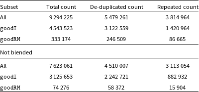
As discussed in Paper Reference ThomsonIII, pixel-wise extraction of spectra means that neighbouring components are not statistically separated as they would be by a true source-finding algorithm. As there are certain scientific use-cases that require isolated components and spectra, we again provide the is_blended_flag column. This flag will be true if any neighbouring components are within 1 PSF width of the given component. In the lower portion of Table 2, we also show the component counts having selected only isolated components where is_blended_flag is false.
We see that the majority of polarised components (187 137 deduplicated components, or 76%) have been flagged as blended. Such components must therefore belong to a PyBDSF source and are therefore extended. In Table 3 we show the number counts of PyBDSF sources for the same subsets as Table 2. From this we can see that the 187 137 deduplicated and blended components in the goodRM subset corresponds to 79 829 sources (or $\sim\!{60}$
%). By comparison, only 181 004, or
$\sim\!{60}$
%). By comparison, only 181 004, or $\sim\!{4.5}\%$
, of the sources in the overall catalogue are flagged as blended. This is not a surprising result, as we expect resolved sources to have a naturally have higher polarisation fractions; they are located further from the centres of their host galaxies and are therefore less subject to in-situ depolarisation. Additionally, we have more resolving elements across an extended source, beam depolarisation is less an of an effect as the source size increases relative the beam.
$\sim\!{4.5}\%$
, of the sources in the overall catalogue are flagged as blended. This is not a surprising result, as we expect resolved sources to have a naturally have higher polarisation fractions; they are located further from the centres of their host galaxies and are therefore less subject to in-situ depolarisation. Additionally, we have more resolving elements across an extended source, beam depolarisation is less an of an effect as the source size increases relative the beam.
Similar to Table 2, except here the number counts are of PyBDSF sources in our catalogue having applied a subset or the is_blended_flag. Here the counts are derived from the exact same subsets as Table 2. We count the number of sources by grouping the catalogue subsets by the source_id column. We note that deduplication makes no difference to the source number counts.

5. Analysis
5.1 Sensitivity and resolution
First, we begin by inspecting the spatial resolution across our survey area. In Figure 3 we show the survey PSF across the sky, and as a function of declination ( $\delta$
). This PSF represents the lowest common resolution across all channels and beams in the cutout around a given source. As discussed in Paper Reference DuchesneIV, scheduling RACS observations within
$\delta$
). This PSF represents the lowest common resolution across all channels and beams in the cutout around a given source. As discussed in Paper Reference DuchesneIV, scheduling RACS observations within $\pm{1}$
h of the meridian provides a spatially contiguous PSF that is primarily declination-dependent. Further, as a snapshot survey, the minor axis (
$\pm{1}$
h of the meridian provides a spatially contiguous PSF that is primarily declination-dependent. Further, as a snapshot survey, the minor axis ( $\theta_{\text{min}}$
) and position angle (
$\theta_{\text{min}}$
) and position angle ( $\theta_{\text{pa}}$
) both depend strongly on the instantaneous uv-coverage of the array for a given azimuth and elevation. For example, field-scale discontinuities seen in Figure 3(c) highlight where gaps in sky coverage, caused by avoiding solar system objects, were filled later in the survey. The major axis (
$\theta_{\text{pa}}$
) both depend strongly on the instantaneous uv-coverage of the array for a given azimuth and elevation. For example, field-scale discontinuities seen in Figure 3(c) highlight where gaps in sky coverage, caused by avoiding solar system objects, were filled later in the survey. The major axis ( $\theta_{\text{maj}}$
) is also larger on the equator where Earth rotation synthesis no longer increases the uv-coverage. We also note that the array layout of ASKAP appears to create a circular PSF at
$\theta_{\text{maj}}$
) is also larger on the equator where Earth rotation synthesis no longer increases the uv-coverage. We also note that the array layout of ASKAP appears to create a circular PSF at $\delta\sim\!{12}^{\circ}$
.
$\delta\sim\!{12}^{\circ}$
.
The point-spread function (PSF, $\theta$
) across the survey area in celestial coordinates. We note that this PSF is the lowest common resolution across all channels in a given cutout cubelet. Panel (a) shows the major axis (
$\theta$
) across the survey area in celestial coordinates. We note that this PSF is the lowest common resolution across all channels in a given cutout cubelet. Panel (a) shows the major axis ( $\theta_{\text{maj}}$
) with a square-root colour scale, panel (b) shows the minor axis also on a square-root colour scale, and panel (c) shows the position angle on a linear scale. In panel (d) we show the PSF specifically against the survey declination (
$\theta_{\text{maj}}$
) with a square-root colour scale, panel (b) shows the minor axis also on a square-root colour scale, and panel (c) shows the position angle on a linear scale. In panel (d) we show the PSF specifically against the survey declination ( $\delta$
). The solid and dashed lines show the median
$\delta$
). The solid and dashed lines show the median $\theta_{\text{maj}}$
and
$\theta_{\text{maj}}$
and $\theta_{\text{min}}$
, respectively. We show the extrema of the these values with the shaded regions.
$\theta_{\text{min}}$
, respectively. We show the extrema of the these values with the shaded regions.

Figure 3. Long description
Panel A: A heatmap showing the major axis of the point-spread function with a square-root color scale. The color gradient ranges from dark purple to yellow, indicating varying values of the major axis in arcseconds. Panel B: A heatmap displaying the minor axis of the point-spread function, also using a square-root color scale. The color gradient ranges from dark purple to red, representing different values of the minor axis in arcseconds. Panel C: A heatmap illustrating the position angle of the point-spread function on a linear scale. The color gradient ranges from dark purple to red, showing the position angle in degrees. Panel D: A line graph showing the point-spread function against the survey declination. The solid blue line represents the median major axis, while the dashed orange line represents the median minor axis. Shaded regions indicate the extrema of these values.
In Paper Reference HaleII and Paper Reference ThomsonIII we elected to use a common resolution of ${25}^{\prime\prime}$
, at the cost of sky area. By way of comparison, here our median PSF major axis is less than
${25}^{\prime\prime}$
, at the cost of sky area. By way of comparison, here our median PSF major axis is less than ${25}^{\prime\prime}$
in the declination range
${25}^{\prime\prime}$
in the declination range $-87^{\circ} \lt\delta\lt+ 30^{\circ}$
. Again we note, however, that we allow our angular resolution to vary for each source cutout. There are a small number of regions where flagging was relatively higher, producing poorer uv-coverage and angular resolution. Our poorest angular resolution occurs at the Northern declination limit of the survey. The median major axis in this region is
$-87^{\circ} \lt\delta\lt+ 30^{\circ}$
. Again we note, however, that we allow our angular resolution to vary for each source cutout. There are a small number of regions where flagging was relatively higher, producing poorer uv-coverage and angular resolution. Our poorest angular resolution occurs at the Northern declination limit of the survey. The median major axis in this region is $\theta_{\text{maj}}=45.9^{\prime\prime}$
, with a maximum value of
$\theta_{\text{maj}}=45.9^{\prime\prime}$
, with a maximum value of $\theta_{\text{maj}}={75.9}^{\prime\prime}$
. Across the majority of our survey area the angular resolution is much better, however, with a median and IQR of our major axis being
$\theta_{\text{maj}}={75.9}^{\prime\prime}$
. Across the majority of our survey area the angular resolution is much better, however, with a median and IQR of our major axis being $14.5 \substack{+5.5\\-1.4}\mathrm{arcsec}$
.
$14.5 \substack{+5.5\\-1.4}\mathrm{arcsec}$
.
We now turn our attention to the survey sensitivity. As described in Section 3.2.2, we extract the robust statistics for rms noise ( $\sigma$
) of the pixels in the local vicinity of each extracted component. In Figure 4 we show the band-averaged
$\sigma$
) of the pixels in the local vicinity of each extracted component. In Figure 4 we show the band-averaged $\sigma$
for Stokes I, Q, and U as well as pI. We measure median and IQR noise across the sky of
$\sigma$
for Stokes I, Q, and U as well as pI. We measure median and IQR noise across the sky of $211 \substack{+150\\-48}\,\mathrm{\mu{Jy}/ PSF}$
,
$211 \substack{+150\\-48}\,\mathrm{\mu{Jy}/ PSF}$
, $194 \substack{+130\\-38}\,\mathrm{\mu{Jy}/ PSF}$
, and
$194 \substack{+130\\-38}\,\mathrm{\mu{Jy}/ PSF}$
, and $194 \substack{+140\\-40}\,\mathrm{\mu{Jy}/ PSF}$
in Stokes I, Stokes Q and U, and pI, respectively. As expected, our average noise is marginally higher than the initial cataloguing due to both our more uniform weighting and the fact that we have not mosaicked adjacent fields.
$194 \substack{+140\\-40}\,\mathrm{\mu{Jy}/ PSF}$
in Stokes I, Stokes Q and U, and pI, respectively. As expected, our average noise is marginally higher than the initial cataloguing due to both our more uniform weighting and the fact that we have not mosaicked adjacent fields.
Fitted, band-averaged rms noise ( $\sigma$
) around each component across the survey area in celestial coordinates in (a) Stokes I, (b) Stokes Q, (c) Stokes U, and (d) polarised intensity (pI). We note that value of
$\sigma$
) around each component across the survey area in celestial coordinates in (a) Stokes I, (b) Stokes Q, (c) Stokes U, and (d) polarised intensity (pI). We note that value of $\sigma_{pI}$
is evaluated after performing RM-synthesis with inverse-variance weighting.
$\sigma_{pI}$
is evaluated after performing RM-synthesis with inverse-variance weighting.

Inspecting the spatial distribution, we note three areas of increased noise. First, a handful of individual fields exhibit outlying noise across the entire observation. As noted in Section 2, a number of target and calibration observations in the initial run of RACS-low3 were impacted by high amounts of flagging. This can be caused by either increased levels of RFI or by a dish rotation unwrap during an observation. As we have not made use of the re-observations, a number of fields in our set have poorer than expected sensitivity. We will be be able to rectify this in a future data release that uses all RACS-low3 observations.
The second area of increased noise we note is in the vicinity of bright sources, particularly in Stokes I. As discussed in Paper Reference DuchesneIV, the impact of bright sources can be significantly improved through peeling or visibility subtraction. Whilst we have not applied these techniques to this data release, we intend to do so in a future release along with other imaging and calibration improvements (Galvin et al. in preparation).
The last area of increased noise in all Stokes parameters is along the Galactic plane. As a snapshot survey, RACS observations cannot recover extended emission with high fidelity, so we expect artefacts along the Galactic plane where bright, extended emission is common. This same extended emission will, to some degree, also be captured in our noise statistics where our noise annulus is much smaller than the scale of the emission itself. Finally, we remark on the lack of such outstanding noise outliers in the pI noise distribution, which appears mostly uniform over the survey area. We can attribute this to our use of inverse-variance weighting in RM-synthesis.
In addition to the rms noise around each component, we also simultaneously compute the background ( $\mu$
) and subtract this channel-wise from each Stokes spectrum (see Section 3.2.2). On average across the sky and band we find backgrounds of
$\mu$
) and subtract this channel-wise from each Stokes spectrum (see Section 3.2.2). On average across the sky and band we find backgrounds of $17 \substack{+110\\-35}\,\mu\text{Jy}/ \mathrm{PSF}$
,
$17 \substack{+110\\-35}\,\mu\text{Jy}/ \mathrm{PSF}$
, $0 \substack{+19\\-18}\,\mathrm{\mu{Jy}/ PSF}$
, and
$0 \substack{+19\\-18}\,\mathrm{\mu{Jy}/ PSF}$
, and $0 \substack{+18\\-18}\,\mathrm{\mu{Jy}/ PSF}$
in Stokes I, Q, and U, respectively. In Figure 5 we show how the band-averaged background is distributed across the sky in Stokes I and pI. Inspecting Stokes I we see that the background is predominantly declination-dependent, with some enhancement along the Galactic plane. Since the spatial distribution of this statistic is clearly correlated with the survey uv-coverage and resulting PSF, we posit that this statistic is mostly capturing residual sidelobe noise in the Stokes I images. In the pI background we can again see the impact on the handful of fields impacted by RFI. Remarkably, we can see diffuse polarised Galactic features, particularly the North Polar Spur, which are commonly seen in single-dish surveys. Rudnick & Brown (Reference Rudnick and Brown2009) previously recovered such features from a re-processing of Reference Taylor, Stil and SunstrumNVSS. We leave detailed analysis of these structures to future work, however we can draw some basic conclusions on the basis of our uv coverage. As noted in Section 3.2.1, we apply a global uv-cut of
$0 \substack{+18\\-18}\,\mathrm{\mu{Jy}/ PSF}$
in Stokes I, Q, and U, respectively. In Figure 5 we show how the band-averaged background is distributed across the sky in Stokes I and pI. Inspecting Stokes I we see that the background is predominantly declination-dependent, with some enhancement along the Galactic plane. Since the spatial distribution of this statistic is clearly correlated with the survey uv-coverage and resulting PSF, we posit that this statistic is mostly capturing residual sidelobe noise in the Stokes I images. In the pI background we can again see the impact on the handful of fields impacted by RFI. Remarkably, we can see diffuse polarised Galactic features, particularly the North Polar Spur, which are commonly seen in single-dish surveys. Rudnick & Brown (Reference Rudnick and Brown2009) previously recovered such features from a re-processing of Reference Taylor, Stil and SunstrumNVSS. We leave detailed analysis of these structures to future work, however we can draw some basic conclusions on the basis of our uv coverage. As noted in Section 3.2.1, we apply a global uv-cut of $200\,\lambda$
which corresponds to largest angular scale of
$200\,\lambda$
which corresponds to largest angular scale of $\sim\!{17}^{\prime}$
. These Galactic polarised emission features must therefore be composed of structures with spatial scales less than this angular size.
$\sim\!{17}^{\prime}$
. These Galactic polarised emission features must therefore be composed of structures with spatial scales less than this angular size.
Fitted, band-averaged background ( $\mu$
) around each component across the survey area in celestial coordinates in (a) Stokes I and (b) polarised intensity (pI). We note that both sub-figures use a square-root colour scale.
$\mu$
) around each component across the survey area in celestial coordinates in (a) Stokes I and (b) polarised intensity (pI). We note that both sub-figures use a square-root colour scale.

5.2 Flux density accuracy
To validate our flux density accuracy in total intensity and linear polarisation we obtain calibrator measurements with the Very Large Array (VLA) from Perley & Butler (Reference Perley and Butler2013) and (Reference Perley and Butler2017) (hereafter Reference Perley and ButlerPB13 and Reference Perley and ButlerPB17), as well as with MeerKAT from Taylor & Legodi (Reference Taylor and Legodi2024, hereafter Reference Taylor and LegodiTL24). These data are presented as integrated flux densities, whereas we only extract pixel-wise peak flux densities. These values should, ideally, be the same for unresolved sources; however, the same will not be true for extended sources. Further, there may be some small differences between our pixel-wise peak and a fitted peak, with the pixel-wise peak being systematically lower. We must also be aware that fractional polarisations can change over time (Reference Perley and ButlerPB13), and can be strongly frequency-dependent. Given these constraints, and the intended purpose of this work as a rotation measure grid, we leave detailed analysis of our flux scale to future work (Galvin et al. in preparation) and we will simply validate our flux scale.
For reference, Reference Perley and ButlerPB17 provide an integrated flux density scale for 20 sources in the range of 50 MHz to 50 GHz, as well as the largest angular scale (LAS) of each source. In polarisation Reference Perley and ButlerPB13 report on four sources (3C48, 3C138, 3C147, and 3C286) in the frequency range of 1–50 GHz at the epoch of December 2010. The work of Reference Taylor and LegodiTL24 provide a curated list of 10 selected broad-band polarisation calibrator sources (out of an initial 98 sources). They present their total intensity and polarisation information at a reference frequency of 1.4 GHz with scaling parameters and standard errors.
We begin our comparison by crossmatching (symmetrically) the calibrator positions to our de-duplicated catalogue. Taking a maximum angular separation of $20^{\prime\prime}$
, we find 11 matches with Reference Perley and ButlerPB17, 9 matches with Reference Taylor and LegodiTL24, and 3 sources from Reference Perley and ButlerPB13. In total intensity we evaluate the models from both Reference Perley and ButlerPB17 and Reference Taylor and LegodiTL24 at our own reference frequency. We show the comparison of the total intensity flux density in the left panel of Figure 6. Excluding sources from Reference Perley and ButlerPB17 with an
$20^{\prime\prime}$
, we find 11 matches with Reference Perley and ButlerPB17, 9 matches with Reference Taylor and LegodiTL24, and 3 sources from Reference Perley and ButlerPB13. In total intensity we evaluate the models from both Reference Perley and ButlerPB17 and Reference Taylor and LegodiTL24 at our own reference frequency. We show the comparison of the total intensity flux density in the left panel of Figure 6. Excluding sources from Reference Perley and ButlerPB17 with an $\text{LAS} \gt 20^{\prime\prime}$
, we find that our total intensity is in agreement with the calibrator measurements within 11%. In polarisation fraction we select the 1.050 GHz data from Reference Perley and ButlerPB13 (which lies within our observed band), and scale the Reference Taylor and LegodiTL24 fraction to our reference frequency with their reported depolarisation term. We show the comparison of the matched fractional polarisations in the right-hand panel of Figure 6. The median fractional difference between our measurements and the calibrators is 16% with a MADstd of 0.4%. Given the above caveats, we are satisfied that our flux scale is accurate to
$\text{LAS} \gt 20^{\prime\prime}$
, we find that our total intensity is in agreement with the calibrator measurements within 11%. In polarisation fraction we select the 1.050 GHz data from Reference Perley and ButlerPB13 (which lies within our observed band), and scale the Reference Taylor and LegodiTL24 fraction to our reference frequency with their reported depolarisation term. We show the comparison of the matched fractional polarisations in the right-hand panel of Figure 6. The median fractional difference between our measurements and the calibrators is 16% with a MADstd of 0.4%. Given the above caveats, we are satisfied that our flux scale is accurate to $\sim\!{15}\%$
; which is in line with the previous epochs of RACS (Paper Reference HaleII; Paper Reference DuchesneIV; Paper Reference DuchesneVI).
$\sim\!{15}\%$
; which is in line with the previous epochs of RACS (Paper Reference HaleII; Paper Reference DuchesneIV; Paper Reference DuchesneVI).
Comparison of Stokes I flux density (left) and polarisation fraction (right) against calibration sources. In both cases, our values are derived from the peak pixel on the source whereas the reference values are integrated. In total intensity, we compare our peak flux density against fitted models from both Reference Perley and ButlerPB17 (circles) and Reference Taylor and LegodiTL24 (squares) evaluated at our reference frequency. The colour scale represents the largest angular size (LAS) as reported by Reference Perley and ButlerPB17. Where the $\text{LAS}\gt 20^{\prime\prime}$
we label the source name. In fractional polarisation we compare against the measurements from Reference Perley and ButlerPB13 (circles) and Reference Taylor and LegodiTL24 (squares). We use the fractional values from Reference Perley and ButlerPB13 at 1.050 GHz, whereas we use the depolarisation term from Reference Taylor and LegodiTL24 to scale to our reference frequency. We colour the points from Reference Perley and ButlerPB13 by our reference frequency and label them with their source name. We show all error bars at
$\text{LAS}\gt 20^{\prime\prime}$
we label the source name. In fractional polarisation we compare against the measurements from Reference Perley and ButlerPB13 (circles) and Reference Taylor and LegodiTL24 (squares). We use the fractional values from Reference Perley and ButlerPB13 at 1.050 GHz, whereas we use the depolarisation term from Reference Taylor and LegodiTL24 to scale to our reference frequency. We colour the points from Reference Perley and ButlerPB13 by our reference frequency and label them with their source name. We show all error bars at $5\sigma$
.
$5\sigma$
.

As a final comparison of our polarisation calibration, we also compare our measured polarisation angles ( $\chi$
) against the Reference Perley and ButlerPB13 and Reference Taylor and LegodiTL24 calibrator surveys. Due to the very Faraday rotation effect we are interested in, the polarisation angle is strongly frequency dependent. As such we de-rotate all polarisation angles to a common reference frequency of 1 GHz, which is in-band for all three surveys. We de-rotate assuming a single RM:
$\chi$
) against the Reference Perley and ButlerPB13 and Reference Taylor and LegodiTL24 calibrator surveys. Due to the very Faraday rotation effect we are interested in, the polarisation angle is strongly frequency dependent. As such we de-rotate all polarisation angles to a common reference frequency of 1 GHz, which is in-band for all three surveys. We de-rotate assuming a single RM:
 \begin{equation} \chi = \chi_r + \text{RM} \left( \lambda^2 - \lambda_r^2 \right),\end{equation}
where $\chi_r$
and
$\chi_r$
and $\lambda_r^2$
are the polarisation angle and wavelength-squared at the reference frequency. As such, any Faraday complexity will result in additional scatter of the de-rotated angle.
$\lambda_r^2$
are the polarisation angle and wavelength-squared at the reference frequency. As such, any Faraday complexity will result in additional scatter of the de-rotated angle.
We show the comparison of our polarisation angles against the calibrator survey values in Figure 7. Against just the data separately from Reference Perley and ButlerPB13 and Reference Taylor and LegodiTL24 the mean and standard deviation of the difference in measured angles is $4.0^{\circ}\pm 0.9^{\circ}$
and
$4.0^{\circ}\pm 0.9^{\circ}$
and ${2}^{\circ}\pm{7}^{\circ}$
, respectively. Combined the difference in angles is
${2}^{\circ}\pm{7}^{\circ}$
, respectively. Combined the difference in angles is ${3}^{\circ}\pm{6}^{\circ}$
. We conclude overall that our absolute polarisation angle calibration is accurate within
${3}^{\circ}\pm{6}^{\circ}$
. We conclude overall that our absolute polarisation angle calibration is accurate within $\sim\!{5}^{\circ}$
.
$\sim\!{5}^{\circ}$
.
Comparison of polarisation angles ( $\chi$
) against calibration sources (as per Figure 6). Data from Reference Perley and ButlerPB13 and Reference Taylor and LegodiTL24 are shown in circles and squares, respectively. Here we have re-rotated all angles to a common reference frequency of 1 GHz using the reported rotation measures from each catalogue. We show error bars at
$\chi$
) against calibration sources (as per Figure 6). Data from Reference Perley and ButlerPB13 and Reference Taylor and LegodiTL24 are shown in circles and squares, respectively. Here we have re-rotated all angles to a common reference frequency of 1 GHz using the reported rotation measures from each catalogue. We show error bars at $5\sigma$
.
$5\sigma$
.

Having satisfied ourselves with the flux scale, we can inspect the distribution of our total and linearly polarised flux density. In Figure 8 we show the 2D histogram of Stokes I against pI for both our goodI and goodRM subsets. For the following values we will report the median with upper and lower ranges given by the $16{\text{th}}$
and
$16{\text{th}}$
and $84{\text{th}}$
percentiles. In the overall goodI subset we find a distribution of
$84{\text{th}}$
percentiles. In the overall goodI subset we find a distribution of $I=6.0 \substack{+20\\-3.6}\,\mathrm{mJy/PSF}$
, and
$I=6.0 \substack{+20\\-3.6}\,\mathrm{mJy/PSF}$
, and $I/\sigma_I=26 \substack{+82\\-15}$
. Where goodI applies but not goodRM the sample is overall lower in Stokes I with
$I/\sigma_I=26 \substack{+82\\-15}$
. Where goodI applies but not goodRM the sample is overall lower in Stokes I with $I=5.4\substack{+13\\-3.0}\,\mathrm{mJy/PSF}$
and
$I=5.4\substack{+13\\-3.0}\,\mathrm{mJy/PSF}$
and $I/\sigma_I=24 \substack{+56\\-12}$
. We can also see the pI is systemically lower for this subset, as expected from our polarised signal-to-noise and leakage cuts. In the
$I/\sigma_I=24 \substack{+56\\-12}$
. We can also see the pI is systemically lower for this subset, as expected from our polarised signal-to-noise and leakage cuts. In the $\texttt{goodRM}$
subset, the distribution in total intensity is
$\texttt{goodRM}$
subset, the distribution in total intensity is $I=55 \substack{+130\\-35}\,\mathrm{mJy/PSF}$
and
$I=55 \substack{+130\\-35}\,\mathrm{mJy/PSF}$
and $I/\sigma_I=230 \substack{+490\\-150}$
. In polarised intensity we find
$I/\sigma_I=230 \substack{+490\\-150}$
. In polarised intensity we find $pI=2.9 \substack{+3.9\\-1.2}\,\mathrm{mJy/PSF}$
with
$pI=2.9 \substack{+3.9\\-1.2}\,\mathrm{mJy/PSF}$
with $pI/\sigma_{pI}=14.0 \substack{+18\\-4.8}$
. In fractional polarisation the distribution is
$pI/\sigma_{pI}=14.0 \substack{+18\\-4.8}$
. In fractional polarisation the distribution is $p=6.1 \substack{+6.4\\-3.7}$
.
$p=6.1 \substack{+6.4\\-3.7}$
.
Finally, we can inspect our fitted in-band spectral indices ( $\alpha$
). We find an error-weighted median of
$\alpha$
). We find an error-weighted median of $\alpha=-0.8\pm0.4$
; consistent with both previous surveys of extragalactic sources (e.g. Condon Reference Condon1992) and the multi-band analysis of RACS from Paper Reference DuchesneVI. In Figure 9(a) we show the distribution of
$\alpha=-0.8\pm0.4$
; consistent with both previous surveys of extragalactic sources (e.g. Condon Reference Condon1992) and the multi-band analysis of RACS from Paper Reference DuchesneVI. In Figure 9(a) we show the distribution of $\alpha$
against total flux density. Overall, there is not a strong error-weighted trend in
$\alpha$
against total flux density. Overall, there is not a strong error-weighted trend in $\alpha$
with flux density until
$\alpha$
with flux density until $I\gtrsim 10{\text{Jy}/\mathrm{PSF}}$
where
$I\gtrsim 10{\text{Jy}/\mathrm{PSF}}$
where $\alpha$
begins to flatten on average. We should also note that a 288 MHz band at
$\alpha$
begins to flatten on average. We should also note that a 288 MHz band at $\sim\!{1}\,\mathrm{GHz}$
is not a particularly long lever arm for determining
$\sim\!{1}\,\mathrm{GHz}$
is not a particularly long lever arm for determining $\alpha$
. As we show in Figure 9(b), below
$\alpha$
. As we show in Figure 9(b), below $I\lesssim 100\,\text{mJy}/\mathrm{PSF}$
the average error on
$I\lesssim 100\,\text{mJy}/\mathrm{PSF}$
the average error on $\alpha$
rises quickly to
$\alpha$
rises quickly to $\sigma_\alpha\sim{1}$
. Above
$\sigma_\alpha\sim{1}$
. Above $I\gtrsim 100\,\mathrm{mJy/PSF}$
the
$I\gtrsim 100\,\mathrm{mJy/PSF}$
the $\sigma_\alpha$
is on the order of
$\sigma_\alpha$
is on the order of $10^{-2}$
. However, as described above, half of our components in the goodI subset have a flux density
$10^{-2}$
. However, as described above, half of our components in the goodI subset have a flux density $I\lt 6\,\,\mathrm{mJy/PSF}$
. Overall, our spectral indices are physically reasonable and certainly sufficient for fractional polarisation analysis through RM synthesis. Users of our reported spectral indices will need to pay careful attention to our reported errors when using them for scientific analysis.
$I\lt 6\,\,\mathrm{mJy/PSF}$
. Overall, our spectral indices are physically reasonable and certainly sufficient for fractional polarisation analysis through RM synthesis. Users of our reported spectral indices will need to pay careful attention to our reported errors when using them for scientific analysis.
Two-dimensional histogram of the Stokes I distribution against pI from our concatenated catalogue. In green we show the density of components from our goodI and not goodRM subset (see Section 4.1), and in purple we show the subset where goodI and goodRM are true. We show contours at the $16\text{th}$
,
$16\text{th}$
, $50\text{th}$
, and
$50\text{th}$
, and $84\text{th}$
percentiles. In dashed lines we show regions of constant fractional polarisation. We shade the forbidden region of over 100% fractional linear polarisation in grey.
$84\text{th}$
percentiles. In dashed lines we show regions of constant fractional polarisation. We shade the forbidden region of over 100% fractional linear polarisation in grey.

5.3 Residual polarisation leakage
As with all widefield ASKAP images, residual widefield polarisation leakage is a critical systemic that can limit the resulting density of our RM grid (Paper Reference ThomsonIII). Further, we also require a method of measuring our residual leakage after correction so that we can successfully select sources with astrophysical, rather than instrumental, linear polarisation. As described in Section 2, our set of RACS-low3 fields were observed entirely with a single set of beamforming weights. This set of weights had holographic measurements made of the beam that we used to correct for the primary beam and off-axis leakage from Stokes I into Q and U.
In a similar process to Paper Reference ThomsonIII, we are able to measure the residual leakage across the field of view of observations by using field sources. In using this technique, we are making the assumption that a majority of sources are not intrinsically linearly polarised. Unlike in DR1, since our data used a single set of beamforming weights, we have the ability to stack across our entire dataset for this measurement.
We begin stacking by selecting high signal-to-noise Stokes I sources from our full catalogue where $I/\sigma_I \gt 20$
. We then form a grid across the instrument field of view in l,m taking 31 bins in each dimension, resulting in bins of
$I/\sigma_I \gt 20$
. We then form a grid across the instrument field of view in l,m taking 31 bins in each dimension, resulting in bins of ${13.5}^{\prime}\times {11.5}^{\prime}$
in size. To minimise the impact of astrophysically polarised sources we first filter using a sigma-clip, and then take the median of the resulting clipped values. We use astropy.stats.sigma_clip to perform the sigma-clip down to a level of
${13.5}^{\prime}\times {11.5}^{\prime}$
in size. To minimise the impact of astrophysically polarised sources we first filter using a sigma-clip, and then take the median of the resulting clipped values. We use astropy.stats.sigma_clip to perform the sigma-clip down to a level of $3\sigma$
with no limit on the number of iterations, and we use the median absolute deviation (MAD) normalised to the standard deviation (MADstd, using astropy.stats.mad_std). We show the resulting distributions of Stokes
$3\sigma$
with no limit on the number of iterations, and we use the median absolute deviation (MAD) normalised to the standard deviation (MADstd, using astropy.stats.mad_std). We show the resulting distributions of Stokes $Q/I$
and
$Q/I$
and $U/I$
in Figure 10(a) and (b), respectively. Inspecting these Figures we can see what appears to be an apparent shift along the m axis, resulting in higher residual leakage towards the edges of the field of view with anti-symmetry about
$U/I$
in Figure 10(a) and (b), respectively. Inspecting these Figures we can see what appears to be an apparent shift along the m axis, resulting in higher residual leakage towards the edges of the field of view with anti-symmetry about $m={0}^{\circ}$
. We found a similar effect in Paper Reference DuchesneIV in the apparent brightness of total intensity sources. There, we also found a flip in the apparent shift depending on where in the sky a given set of primary beams where determined and then applied. Here, however, we find that further sub-dividing our catalogue reduces the residual leakage ‘signal’ to a point where concrete analysis is no longer viable. Despite this, it is still worthy of note that our data again shows this affect with ASKAP data, and should be noted for future surveys and observations.
$m={0}^{\circ}$
. We found a similar effect in Paper Reference DuchesneIV in the apparent brightness of total intensity sources. There, we also found a flip in the apparent shift depending on where in the sky a given set of primary beams where determined and then applied. Here, however, we find that further sub-dividing our catalogue reduces the residual leakage ‘signal’ to a point where concrete analysis is no longer viable. Despite this, it is still worthy of note that our data again shows this affect with ASKAP data, and should be noted for future surveys and observations.
To determine the leakage from I into p we form the polarised intensity surface from our $Q/I$
and
$Q/I$
and $U/I$
grids, which we show in Figure 10(c). For the purposes of our catalogue we collapse the l, m axes into a simple angular separation (
$U/I$
grids, which we show in Figure 10(c). For the purposes of our catalogue we collapse the l, m axes into a simple angular separation ( $\vartheta$
) and bin the resulting values to minimise the impact of variance in our leakage surface. Finally, we fit an empirical model to this data of the functional form:
$\vartheta$
) and bin the resulting values to minimise the impact of variance in our leakage surface. Finally, we fit an empirical model to this data of the functional form:
 \begin{equation} p_{\text{leak}} = a e^{b\vartheta} +c,\end{equation}
where our fitted values are $a=2.7\times10^{-7}$
,
$a=2.7\times10^{-7}$
, $b=2.58$
, and
$b=2.58$
, and $c=1.16\times10^{-3}$
. This informs us that, over most of the field of view, the residual leakage is
$c=1.16\times10^{-3}$
. This informs us that, over most of the field of view, the residual leakage is $\sim\!{0.1}\%$
. This is an order of magnitude improvement over our DR1 result (Paper Reference ThomsonIII). Beyond a separation of
$\sim\!{0.1}\%$
. This is an order of magnitude improvement over our DR1 result (Paper Reference ThomsonIII). Beyond a separation of $\sim\!{2.5}^{\circ}$
from the tile centre the residual leakage climbs to
$\sim\!{2.5}^{\circ}$
from the tile centre the residual leakage climbs to $\sim\!{1}\%$
. For each row in our catalogue we evaluate the fitted model and report the resulting value in the leakage column.
$\sim\!{1}\%$
. For each row in our catalogue we evaluate the fitted model and report the resulting value in the leakage column.
5.4 Rotation measure accuracy and analysis
To validate our determined RMs we compare with a collection of historical RM surveys. We begin with version 1.2.0 of the RMTable compilation (Van Eck et al. Reference Van Eck2023, hereafter Reference Van EckRMTable). To this we add version 9 of the ATNF Pulsar Catalogue SQLite databaseFootnote i (Manchester et al. Reference Manchester, Hobbs, Teoh and Hobbs2005; Hobbs et al. Reference Hobbs, Kapur and Toomey2025, hereafter Reference Manchester, Hobbs, Teoh and HobbsPSRCAT), as well as catalogues from Paper Reference ThomsonIII, Reference Taylor and LegodiTL24, and Loi et al. (Reference Loi2025). We cross-match this combined collection symmetrically with our de-duplicated, goodRM catalogue using astropy. coordinates.SkyCoord.match_to_catalog_sky with a ma- ximum separation based on the angular resolution of the respective surveys. We take the maximum of either our own or the external catalogue’s PSF major axis, and set the maximum angular separation to be twice that value.
Stokes I spectral indices ( $\alpha$
). In (a) we show the 2D histogram of
$\alpha$
). In (a) we show the 2D histogram of $\alpha$
against Stokes I flux density from our concatenated catalogue in the range
$\alpha$
against Stokes I flux density from our concatenated catalogue in the range $-5\leq\alpha\leq5$
. In the black solid and shaded region we show the error-weighted mean (
$-5\leq\alpha\leq5$
. In the black solid and shaded region we show the error-weighted mean ( $\mu$
) and standard deviation (
$\mu$
) and standard deviation ( $\sigma$
) of the
$\sigma$
) of the $\alpha$
in bins of flux density. In the vertical red dashed line we show where
$\alpha$
in bins of flux density. In the vertical red dashed line we show where $\alpha=-0.8$
. We note that, due to our hierarchical fitting method, some models are fit with a flat spectral index, which effectively sets
$\alpha=-0.8$
. We note that, due to our hierarchical fitting method, some models are fit with a flat spectral index, which effectively sets $\alpha=0$
. This results in the sharp feature in the distribution at
$\alpha=0$
. This results in the sharp feature in the distribution at $\alpha=0$
. In (b) we show the error on the spectral index
$\alpha=0$
. In (b) we show the error on the spectral index $\sigma_\alpha$
as function of Stokes I. Each error bar shows the median and with 16th and 84th percentile range.
$\sigma_\alpha$
as function of Stokes I. Each error bar shows the median and with 16th and 84th percentile range.

Despite their common format (thanks to the RMTable schema), the construction of each catalogue may be vastly different. For example, the nominal frequency coverage, the RM algorithm used, and application of ionospheric correction may all differ greatly between catalogues. Further, true RM variation may occur between the epochs of each component observation (e.g. Anderson et al. Reference Anderson2019). As such we perform our comparison on the basis of each individual catalogue in our collection. For the purpose of comparison we will be analysing the distribution of differences between our RM and the historical RM ( $\Delta\text{RM}$
) and the error on this difference (
$\Delta\text{RM}$
) and the error on this difference ( $\sigma_{\Delta\text{RM}}$
). If the variance in
$\sigma_{\Delta\text{RM}}$
). If the variance in $\Delta\text{RM}$
was purely caused by Gaussian noise, and if the errors are correctly measured, we would expect to see an error-normalised difference in RM of
$\Delta\text{RM}$
was purely caused by Gaussian noise, and if the errors are correctly measured, we would expect to see an error-normalised difference in RM of $\Delta\text{RM}/\sigma_{\Delta\text{RM}}=0\pm1$
. The error normalised difference between any pair of uncorrelated values (X) is given by
$\Delta\text{RM}/\sigma_{\Delta\text{RM}}=0\pm1$
. The error normalised difference between any pair of uncorrelated values (X) is given by
 \begin{equation} \frac{\Delta X}{\sigma_{\Delta X}} = \frac{X_1 - X_2}{\sqrt{\sigma_{X_1}^2 + \sigma_{X_2}^2}}, \end{equation}
where here we substitute $X=\text{RM}$
and subscripts 1 and 2 denote the first and second components in a pair, respectively.
$X=\text{RM}$
and subscripts 1 and 2 denote the first and second components in a pair, respectively.
By far the largest catalogue in our historical collection, by both number of RMs and areal coverage, is from Reference Taylor, Stil and SunstrumNVSS. Since RMs in this catalogue were computed from two narrowly-spaced frequencies, the reported RMs may suffer from the $n\pi$
ambiguity. Indeed, this has been found to be the case; Ma et al. (Reference Ma2019) report a lower limit of 50 RMs. A single-wrap (
$n\pi$
ambiguity. Indeed, this has been found to be the case; Ma et al. (Reference Ma2019) report a lower limit of 50 RMs. A single-wrap ( $n=1$
) error corresponds to
$n=1$
) error corresponds to $\pm 652.9\,\mathrm{rad\,m}^{-2}$
. Upon cross-matching with our catalogue, in addition to components which are centred
$\pm 652.9\,\mathrm{rad\,m}^{-2}$
. Upon cross-matching with our catalogue, in addition to components which are centred $\Delta\text{RM}=0 \, \,\mathrm{rad\,m}^{-2}$
, we find two populations centred on expected
$\Delta\text{RM}=0 \, \,\mathrm{rad\,m}^{-2}$
, we find two populations centred on expected $1\pi$
wrap error. As such, we make a correction to the matched Reference Taylor, Stil and SunstrumNVSS catalogue; we take any component where
$1\pi$
wrap error. As such, we make a correction to the matched Reference Taylor, Stil and SunstrumNVSS catalogue; we take any component where $|\Delta\text{RM}|\gt 400\,\mathrm{rad\,m}^{-2}$
and subtract
$|\Delta\text{RM}|\gt 400\,\mathrm{rad\,m}^{-2}$
and subtract $\pm 652.9\,\mathrm{rad\,m}^{-2}$
(with the appropriate sign) to bring all Reference Taylor, Stil and SunstrumNVSS components into a single distribution around
$\pm 652.9\,\mathrm{rad\,m}^{-2}$
(with the appropriate sign) to bring all Reference Taylor, Stil and SunstrumNVSS components into a single distribution around $\Delta\text{RM}= 0\,\mathrm{rad\,m}^{-2}$
. Overall, we find
$\Delta\text{RM}= 0\,\mathrm{rad\,m}^{-2}$
. Overall, we find $30\,183$
matching components with Reference Taylor, Stil and SunstrumNVSS, 146 of which we correct for the
$30\,183$
matching components with Reference Taylor, Stil and SunstrumNVSS, 146 of which we correct for the $n\pi$
ambiguity.
$n\pi$
ambiguity.
Residual leakage across the field of view in RACS-low3. Panels (a) and (b) show our estimate of the residual leakage from Stokes I into Stokes Q and U in the telescope frame, respectively. We combine these to produce the leakage in fractional polarisation (p), which we show in panel (c). We flatten this fractional map to view the residual leakage as a function of angular separation from the tile centre, which we show in panel (d). In this panel we give the fractional leakage as a percentage on a logarithmic scale, and we produce a 2D histogram where the points are over-dense. In the solid purple line we show our empirical fit to the residual leakage which has the functional form: $ae^{b\vartheta}+c$
where
$ae^{b\vartheta}+c$
where $\vartheta$
is the angular separation. Our fitted values are
$\vartheta$
is the angular separation. Our fitted values are $a=2.7\times10^{-7}$
,
$a=2.7\times10^{-7}$
, $b=2.58$
, and
$b=2.58$
, and $c=1.16\times10^{-3}$
.
$c=1.16\times10^{-3}$
.

Having queried the Reference Manchester, Hobbs, Teoh and HobbsPSRCAT database, we retrieve 3 595 pulsars with reported coordinates. After cross-matching with our catalogue, and removing duplicate matches for multiple pulsars which match the same RACS component, we find 133 matches to known pulsars. Of these, 6 do not have reported RMs; we show our RMs, along with our component name and the pulsar name, in Table 4. We show the distribution of pulsar RMs against our own for the remaining 127 pulsars in Figure 11. Initially, we found that a single pulsar, J1406-5806, was outlying from the 1:1 line. On closer inspection, we find that the offset from our measured RM is almost exactly the twice magnitude of the RM. As such, we assume this to be a sign error from the original catalogue of Kramer et al. (Reference Kramer2003) and we invert the sign of the pulsar value to match our own. Having made this single correction, the overall distribution of RM between the two datasets is very tight, with the error-normalised difference in RM $\Delta\text{RM}/\sigma_{\Delta\text{RM}}=0.4 \substack{+1.7\\-1.5}$
.
$\Delta\text{RM}/\sigma_{\Delta\text{RM}}=0.4 \substack{+1.7\\-1.5}$
.
Having made the correction described above, we now look to comparing our RMs with the historical compilation in bulk. In Figure 12 we show the distribution of $\Delta\text{RM}/\sigma_{\Delta\text{RM}}$
for each catalogue. In this Figure we also denote the number of crossmatches to our components, as well as the nominal reference frequency of each catalogue. Deep investigation of each matched component is beyond the scope of this work, however we note a number of interesting features. Overall, our measured RMs are in bulk agreement with the historical compilation, with a handful of outliers in each catalogue.
$\Delta\text{RM}/\sigma_{\Delta\text{RM}}$
for each catalogue. In this Figure we also denote the number of crossmatches to our components, as well as the nominal reference frequency of each catalogue. Deep investigation of each matched component is beyond the scope of this work, however we note a number of interesting features. Overall, our measured RMs are in bulk agreement with the historical compilation, with a handful of outliers in each catalogue.
To investigate whether these outliers are caused by systematics we first repeat our cross-matching analysis, taking our reference catalogue to be Reference Taylor, Stil and SunstrumNVSS and then Reference SchnitzelerS-PASS/ATCA. We find similar results as when we use SPICE-RACS DR2 as the reference catalogue. A deep analysis of the differences between each catalogue is beyond the scope of this work, but there are a few historical features to note. Catalogues which sample relatively few values of $\lambda^2$
, such as Reference Taylor, Stil and SunstrumNVSS, as subject to
$\lambda^2$
, such as Reference Taylor, Stil and SunstrumNVSS, as subject to $n\pi$
ambiguity errors. The nominal
$n\pi$
ambiguity errors. The nominal $\lambda^2$
coverage, which we indicate in Figure 12, can affect which RM components are detected. For example, at long wavelengths components can become depolarised, whereas at short wavelength multiple components can become unresolved. Additionally, some RM components detected with sufficient signal-to-noise can be observed to vary over time (Anderson et al. Reference Anderson2019).
$\lambda^2$
coverage, which we indicate in Figure 12, can affect which RM components are detected. For example, at long wavelengths components can become depolarised, whereas at short wavelength multiple components can become unresolved. Additionally, some RM components detected with sufficient signal-to-noise can be observed to vary over time (Anderson et al. Reference Anderson2019).
We note a larger number of outlying RMs in comparison with Reference SchnitzelerS-PASS/ATCA, the previous largest Southern sky RM survey. We can suggest a few reasons for disagreement between our RM values. First, the angular resolution of Reference SchnitzelerS-PASS/ATCA is relatively coarse ( $\sim\!{2}^{\prime}$
) which makes correctly matching components difficult. Second, the higher observed band (1–3 GHz) means that Reference SchnitzelerS-PASS/ATCA is less sensitive to depolarisation effects, and may be finding a different peak in the Faraday spectrum. Additionally, Reference SchnitzelerS-PASS/ATCA also used their own QU-fitting approach applied directly to visibilities, rather than RM-synthesis of extracted image spectra. Finally, inspecting the distribution of RMs of Reference SchnitzelerS-PASS/ATCA against both our own RMs and NVSSReference Taylor, Stil and SunstrumNVSS, we see that Reference SchnitzelerS-PASS/ATCA reports many more RMs above
$\sim\!{2}^{\prime}$
) which makes correctly matching components difficult. Second, the higher observed band (1–3 GHz) means that Reference SchnitzelerS-PASS/ATCA is less sensitive to depolarisation effects, and may be finding a different peak in the Faraday spectrum. Additionally, Reference SchnitzelerS-PASS/ATCA also used their own QU-fitting approach applied directly to visibilities, rather than RM-synthesis of extracted image spectra. Finally, inspecting the distribution of RMs of Reference SchnitzelerS-PASS/ATCA against both our own RMs and NVSSReference Taylor, Stil and SunstrumNVSS, we see that Reference SchnitzelerS-PASS/ATCA reports many more RMs above $|\text{RM}|\gtrsim 1\,000\,\mathrm{rad\,m}^{-2}$
. Such high RM values likely cause strong depolarisation in our sub-1 GHz spectra.
$|\text{RM}|\gtrsim 1\,000\,\mathrm{rad\,m}^{-2}$
. Such high RM values likely cause strong depolarisation in our sub-1 GHz spectra.
The catalogue with the largest bulk difference from our values is from Livingston et al. (Reference Livingston, McClure-Griffiths, Gaensler, Seta and Alger2021). This work targeted sources towards the Galactic centre, and found significant Faraday complexity in their sample. In effect, this large dispersion of $\Delta\text{RM}/\sigma_{\Delta\text{RM}}$
complements their in-band Faraday complexity result. These sources would make excellent targets for follow up monitoring observations and searches of astrophysical variability and Faraday complexity.
$\Delta\text{RM}/\sigma_{\Delta\text{RM}}$
complements their in-band Faraday complexity result. These sources would make excellent targets for follow up monitoring observations and searches of astrophysical variability and Faraday complexity.
As final check for systematic issues in our own catalogue, we perform a statistical feature comparison to identify which columns in our matched catalogue are predictors for large differences in RM relative to matched catalogues. We split our catalogue in two groups based on the value $\Delta\text{RM}/\sigma_{\Delta\text{RM}}$
.
$\Delta\text{RM}/\sigma_{\Delta\text{RM}}$
.
For numerical values we obtain a p-value from a Mann-Whitney U test (Mann & Whitney Reference Mann and Whitney1947, using scipy.stats. mannwhitneyu) and compute the Cohen’s d value (Cohen Reference Cohen1988) to identify significant columns. Similarly for ‘categorial’ columns (such as the matched external catalogue name), we obtain a p-value from a chi-squared test (using scipy. stats.chi2_contingency) and Cramér’s V value. We then correct the p-values for multiple test false detections with Benjamini-Hochberg (Benjamini & Hochberg Reference Benjamini and Hochberg1995) correction (using statsmodels.stats.multitest.multipletests from Seabold & Perktold Reference Seabold and Perktold2010). We then filter the resulting tests using $p\lt0.05$
combined with either
$p\lt0.05$
combined with either $d\geq0.5$
or
$d\geq0.5$
or $V\geq0.1$
. Here we take the d and V values to measure the effect size for numerical and categorial columns, respectively.
$V\geq0.1$
. Here we take the d and V values to measure the effect size for numerical and categorial columns, respectively.
To we select a value of $\Delta\text{RM}/\sigma_{\Delta\text{RM}}=5$
on which to split our matched catalogue. Following the above filtering, we find the following columns are statistically significant between the two groups (sorted by effect size): other_reffreq_pol, stokesI, sigma_add, rm_width, peak_I_flux_err, peak_I_flux, total_I_flux_err, total_I_flux, rm_diff_err, fdf_noise_mad, other_rm_err, snr_polint, fracpol, and other_cat_name. We see that the strongest indicator of effect size is the reference frequency of the catalogue we match to. Additionally, our RM-complexity metrics are two of the strongest predictors of difference between the two groups. We discuss our complexity metrics in detail in Section 5.5, however here we will note that we expect all the columns list here to correlate strongly with Faraday complexity except for rm_diff_err (which is
$\Delta\text{RM}/\sigma_{\Delta\text{RM}}=5$
on which to split our matched catalogue. Following the above filtering, we find the following columns are statistically significant between the two groups (sorted by effect size): other_reffreq_pol, stokesI, sigma_add, rm_width, peak_I_flux_err, peak_I_flux, total_I_flux_err, total_I_flux, rm_diff_err, fdf_noise_mad, other_rm_err, snr_polint, fracpol, and other_cat_name. We see that the strongest indicator of effect size is the reference frequency of the catalogue we match to. Additionally, our RM-complexity metrics are two of the strongest predictors of difference between the two groups. We discuss our complexity metrics in detail in Section 5.5, however here we will note that we expect all the columns list here to correlate strongly with Faraday complexity except for rm_diff_err (which is $\sigma_{\Delta\text{RM}}$
) and other_cat_name (the name of the external catalogue).
$\sigma_{\Delta\text{RM}}$
) and other_cat_name (the name of the external catalogue).
The sign of the d-value also indicates the relative magnitude of parameters between our subsets. For our test, a positive d-value indicates the parameter is larger in in the $\Delta\text{RM}/\sigma_{\Delta\text{RM}}\gt5$
set, whereas a negative value indicates it is smaller. Of the catalogue columns listed above only rm_diff_err, other_rm_err, and fracpol have a negative d-value, whereas all others are positive. Smaller values of rm_diff_err and other_rm_err could indicate either underestimated errors in the external catalogue. Such a case could arise from low-frequency observations where the narrow RMSF provides highly precise RMs such that the error budget becomes dominated by systematic errors which are harder to quantify. Overall, however, the d-value of other_reffreq_pol is positive, indicating that the reference frequency of the external catalogue is larger than ours in the
$\Delta\text{RM}/\sigma_{\Delta\text{RM}}\gt5$
set, whereas a negative value indicates it is smaller. Of the catalogue columns listed above only rm_diff_err, other_rm_err, and fracpol have a negative d-value, whereas all others are positive. Smaller values of rm_diff_err and other_rm_err could indicate either underestimated errors in the external catalogue. Such a case could arise from low-frequency observations where the narrow RMSF provides highly precise RMs such that the error budget becomes dominated by systematic errors which are harder to quantify. Overall, however, the d-value of other_reffreq_pol is positive, indicating that the reference frequency of the external catalogue is larger than ours in the $\Delta\text{RM}/\sigma_{\Delta\text{RM}}\gt5$
. As discussed above, higher frequency observations are more sensitive to Faraday thick features, meaning they will measure measure a different RM in the presence of depolarisation effects (see discussion in e.g. Van Eck et al. Reference Van Eck2017). Finally, we note smaller values of fracpol in the
$\Delta\text{RM}/\sigma_{\Delta\text{RM}}\gt5$
. As discussed above, higher frequency observations are more sensitive to Faraday thick features, meaning they will measure measure a different RM in the presence of depolarisation effects (see discussion in e.g. Van Eck et al. Reference Van Eck2017). Finally, we note smaller values of fracpol in the $\Delta\text{RM}/\sigma_{\Delta\text{RM}}\gt5$
set. This difference, combined with larger relative values of total intensity, could be an indicator of residual polarisation leakage in our catalogued RMs. We investigate the internal reliability of our RM catalogue in Section 5.6.
$\Delta\text{RM}/\sigma_{\Delta\text{RM}}\gt5$
set. This difference, combined with larger relative values of total intensity, could be an indicator of residual polarisation leakage in our catalogued RMs. We investigate the internal reliability of our RM catalogue in Section 5.6.
Overall, we conclude that the majority of the outliers we see are caused by systematic differences between our survey and historical catalogues, or multiple components in our Faraday spectrum, as indicated by Faraday complexity.
Known pulsars with new RMs in SPICE-RACS DR2.

Our rotation measures (RM) cross-matched to 127 pulsar RMs from Reference Manchester, Hobbs, Teoh and HobbsPSRCAT. Where scatter points are over-dense we show the density of points in the colourscale. We show the 1:1 relation in the red, dashed lined.

5.4.1 SPICE-RACS DR2 RM grid
Having validated our RMs against previous observations, we now look at our own dataset directly. First, we we look at the distribution of our RMs as a function of polarised signal-to-noise ( $\mathcal{L}=pI/\sigma_{pI}$
). We show this distribution in Figure 13. Similar to the distribution we saw in Paper Reference ThomsonIII, the distribution of RM continues smoothly below the nominal cut of
$\mathcal{L}=pI/\sigma_{pI}$
). We show this distribution in Figure 13. Similar to the distribution we saw in Paper Reference ThomsonIII, the distribution of RM continues smoothly below the nominal cut of $8\sigma$
in pI. In this case, however, we see that the apparently smooth RM distribution continues down to
$8\sigma$
in pI. In this case, however, we see that the apparently smooth RM distribution continues down to $\sim\!{5}\sigma$
before abruptly spanning the entire possible range of RMs. In Paper Reference ThomsonIII, this occurred at
$\sim\!{5}\sigma$
before abruptly spanning the entire possible range of RMs. In Paper Reference ThomsonIII, this occurred at $\sim\!{7}\sigma$
(see Figure 8 of that work). Here we can also see the effect of our two channelisations, namely 36 or 72 channels, in the sharp cuts at RM
$\sim\!{7}\sigma$
(see Figure 8 of that work). Here we can also see the effect of our two channelisations, namely 36 or 72 channels, in the sharp cuts at RM $\sim\!{600}\,\mathrm{rad}\,\mathrm{m}^{-2}$
and
$\sim\!{600}\,\mathrm{rad}\,\mathrm{m}^{-2}$
and $\sim\!{1}\,200\,\mathrm{rad\,m}^{-2}$
.
$\sim\!{1}\,200\,\mathrm{rad\,m}^{-2}$
.
To investigate where this unphysical distribution of RMs occurs, we slice our catalogue into subsets of $\mathcal{L}$
values. We form bins with a lower edge
$\mathcal{L}$
values. We form bins with a lower edge $\mathcal{L}_{\text{min}}$
and a width
$\mathcal{L}_{\text{min}}$
and a width $\delta_{\mathcal{L}}$
such that a bin is defined by
$\delta_{\mathcal{L}}$
such that a bin is defined by $\mathcal{L}_{\text{min}} \leq \mathcal{L} \lt \mathcal{L} + \delta_{\mathcal{L}}$
. We chose lower edges in the range
$\mathcal{L}_{\text{min}} \leq \mathcal{L} \lt \mathcal{L} + \delta_{\mathcal{L}}$
. We chose lower edges in the range $3\leq \mathcal{L}_{\text{min}} \leq 10$
and take
$3\leq \mathcal{L}_{\text{min}} \leq 10$
and take $\delta_{\mathcal{L}}=0.1$
. In the upper panels of Figure 14 we show the cumulative distribution function (CDF) of RM for each signal-to-noise ratio. To compare the distributions we take a two-sample Kolmogorov-Smirnov (KS) test between the highest
$\delta_{\mathcal{L}}=0.1$
. In the upper panels of Figure 14 we show the cumulative distribution function (CDF) of RM for each signal-to-noise ratio. To compare the distributions we take a two-sample Kolmogorov-Smirnov (KS) test between the highest $\mathcal{L}$
bin and all other bins. In the bottom panel of Figure 14 we show both the KS statistic as well as the p-value corresponding to the null hypothesis. In this case the null hypothesis is that the two samples were drawn from the same distribution; if the p-value is below a selected threshold we can reject the null hypothesis and conclude that the samples were drawn from different distributions. If we take a threshold p-value of 0.05, corresponding to a confidence of 95%, we find that for
$\mathcal{L}$
bin and all other bins. In the bottom panel of Figure 14 we show both the KS statistic as well as the p-value corresponding to the null hypothesis. In this case the null hypothesis is that the two samples were drawn from the same distribution; if the p-value is below a selected threshold we can reject the null hypothesis and conclude that the samples were drawn from different distributions. If we take a threshold p-value of 0.05, corresponding to a confidence of 95%, we find that for $\mathcal{L}_{\text{min}}$
below
$\mathcal{L}_{\text{min}}$
below $5.5\sigma$
we can reject null the hypothesis. Stated the other way, for each bin where
$5.5\sigma$
we can reject null the hypothesis. Stated the other way, for each bin where $\mathcal{L}_{\text{min}}\geq 5.5$
we cannot discriminate between the distribution of RM in that bin and the distribution in the
$\mathcal{L}_{\text{min}}\geq 5.5$
we cannot discriminate between the distribution of RM in that bin and the distribution in the $10\sigma$
bin.
$10\sigma$
bin.
The difference in RM ( $\Delta\text{RM}$
) between SPICE-RACS DR2 matched with an external catalogue, normalised by the error in the
$\Delta\text{RM}$
) between SPICE-RACS DR2 matched with an external catalogue, normalised by the error in the $\Delta\text{RM}$
(
$\Delta\text{RM}$
( $\sigma_{\Delta\text{RM}}$
). The majority of catalogues listed above are components of Reference Van EckRMTable v1.2.0. To this we have added the catalogues from Paper Reference ThomsonIII, Reference Taylor and LegodiTL24, Loi et al. (Reference Loi2025), and the Reference Manchester, Hobbs, Teoh and HobbsPSRCAT (Manchester et al. Reference Manchester, Hobbs, Teoh and Hobbs2005 in the axis label). We present the distribution of the
$\sigma_{\Delta\text{RM}}$
). The majority of catalogues listed above are components of Reference Van EckRMTable v1.2.0. To this we have added the catalogues from Paper Reference ThomsonIII, Reference Taylor and LegodiTL24, Loi et al. (Reference Loi2025), and the Reference Manchester, Hobbs, Teoh and HobbsPSRCAT (Manchester et al. Reference Manchester, Hobbs, Teoh and Hobbs2005 in the axis label). We present the distribution of the $\Delta\text{RM}/\sigma_{\Delta\text{RM}}$
for each catalogue as a box-and-whisker diagram (Spear Reference Spear1952; Tukey Reference Tukey1977). In the thick lines we show the box-and-whisker distribution between the 16th and 84th percentiles. In the thin lines we show the extrema of the distribution. The vertical dotted and dashed lines show the
$\Delta\text{RM}/\sigma_{\Delta\text{RM}}$
for each catalogue as a box-and-whisker diagram (Spear Reference Spear1952; Tukey Reference Tukey1977). In the thick lines we show the box-and-whisker distribution between the 16th and 84th percentiles. In the thin lines we show the extrema of the distribution. The vertical dotted and dashed lines show the $\pm1\sigma$
and
$\pm1\sigma$
and $\pm5\sigma$
ranges, respectively. For perfectly normally-distributed errors we would expect the inner box of each distribution to lie within the
$\pm5\sigma$
ranges, respectively. For perfectly normally-distributed errors we would expect the inner box of each distribution to lie within the $\pm1\sigma$
range. We have sorted each catalogue by the number of matches with SPICE-RACS DR2 from most at the bottom to least at the top, with the number of matches listed on the right-hand axis. The corresponding authorship name for each catalogue is given on the left axis. We also colour each distribution by its corresponding reference wavelength-squared (
$\pm1\sigma$
range. We have sorted each catalogue by the number of matches with SPICE-RACS DR2 from most at the bottom to least at the top, with the number of matches listed on the right-hand axis. The corresponding authorship name for each catalogue is given on the left axis. We also colour each distribution by its corresponding reference wavelength-squared ( $\lambda^2$
) with a logarithmic colour scale. We note that same catalogues do not contain a single, homogeneous reference wavelength-squared which we cannot represent in this figure. If a catalogue does have reported reference wavelength-squared, we colour the lines grey. Note that the references for the sub-catalogues of Reference Van EckRMTable are given in Van Eck et al. (Reference Van Eck2023). We also enumerate all such references in our own reference list.
$\lambda^2$
) with a logarithmic colour scale. We note that same catalogues do not contain a single, homogeneous reference wavelength-squared which we cannot represent in this figure. If a catalogue does have reported reference wavelength-squared, we colour the lines grey. Note that the references for the sub-catalogues of Reference Van EckRMTable are given in Van Eck et al. (Reference Van Eck2023). We also enumerate all such references in our own reference list.

Two-dimesional histograms of the absolute value of rotation measure ( $|\text{RM}|$
) against polarised intensity signal-to-noise (
$|\text{RM}|$
) against polarised intensity signal-to-noise ( $pI/\sigma_{pI}$
). We colour the region where our goodRM subset applies in purple, and in green we shade where goodI applies but not goodRM (see Section 4.1). In the vertical dashed line we show divider between goodI and goodRM where
$pI/\sigma_{pI}$
). We colour the region where our goodRM subset applies in purple, and in green we shade where goodI applies but not goodRM (see Section 4.1). In the vertical dashed line we show divider between goodI and goodRM where $pI/\sigma_{pI}=8$
.
$pI/\sigma_{pI}=8$
.

A comparison of distributions in polarised signal-to-noise ( $\mathcal{L}=pI/\sigma_{pI}$
) bins. Here the value
$\mathcal{L}=pI/\sigma_{pI}$
) bins. Here the value $\mathcal{L}_{\text{min}}$
gives the left (inclusive) edge of a bin, with a width of 0.1. The upper and middle panels show the cumulative distribution function (CDF) of RM in each bin, where the colour of each line corresponds to the
$\mathcal{L}_{\text{min}}$
gives the left (inclusive) edge of a bin, with a width of 0.1. The upper and middle panels show the cumulative distribution function (CDF) of RM in each bin, where the colour of each line corresponds to the $\mathcal{L}_{\text{min}}$
bin. The middle panel rescaled to highlight small separations between the CDFs at large (postive) RMs. The bottom panel shows the results of a two-sample Kolmogorov-Smirnov (KS) test between each bin and the highest signal-to-noise bin. In orange we show the value of the KS statistic, and in blue we show the associated p-values. The horizontal, dotted line shows where the p-value is 0.05, and the vertical, dashed line shows the lowest
$\mathcal{L}_{\text{min}}$
bin. The middle panel rescaled to highlight small separations between the CDFs at large (postive) RMs. The bottom panel shows the results of a two-sample Kolmogorov-Smirnov (KS) test between each bin and the highest signal-to-noise bin. In orange we show the value of the KS statistic, and in blue we show the associated p-values. The horizontal, dotted line shows where the p-value is 0.05, and the vertical, dashed line shows the lowest $\mathcal{L}_{\text{min}}$
bin for which we cannot reject the null-hypothesis (see text in Section 5.4.1 for further details).
$\mathcal{L}_{\text{min}}$
bin for which we cannot reject the null-hypothesis (see text in Section 5.4.1 for further details).

A robust analytic formalism for detection thresholds in linear polarisation and RM-synthesis was derived by Hales et al. (Reference Hales, Gaensler, Norris and Middelberg2012), with similar discussions in Macquart et al. (Reference Macquart, Ekers, Feain and Johnston-Hollitt2012) and George et al. (Reference George, Stil and Keller2012). Equation (31) of Hales et al. (Reference Hales, Gaensler, Norris and Middelberg2012) provides the required value of $\mathcal{L}$
for an equivalent false detection in a Gaussian distribution, with signal-to-noise ratio (
$\mathcal{L}$
for an equivalent false detection in a Gaussian distribution, with signal-to-noise ratio ( $\mathcal{G}$
):
$\mathcal{G}$
):
 \begin{equation} \mathcal{L} = \sqrt{-2 \ln\left\{1 - \left[\text{erf}\left(\frac{\mathcal{G}}{\sqrt{2}}\right)\right]^{1/N_{\text{FDF}}}\right\}},\end{equation}
and inversely (Hales et al. Reference Hales, Gaensler, Norris and Middelberg2012, Equation 30),
 \begin{equation} \mathcal{G}=\sqrt{2}\text{erf}^{-1}\left\{\left[1-\exp{\left(\frac{-\mathcal{L}^2}{2}\right)}\right]^{N_{\text{FDF}}}\right\}.\end{equation}
Here erf and $\text{erf}^{-1}$
are the error function and its inverse, respectively, and
$\text{erf}^{-1}$
are the error function and its inverse, respectively, and $N_{\text{FDF}}$
is the number of independent samples across the FDF given by:
$N_{\text{FDF}}$
is the number of independent samples across the FDF given by:
 \begin{equation} N_{\text{FDF}} = \frac{2\phi_{\text{max}}}{\delta\phi} \approx \frac{\Delta\lambda^2}{\delta\lambda^2}.\end{equation}
Here, $\phi_{\text{max}}$
and
$\phi_{\text{max}}$
and $\delta\phi$
are as defined in Section 3.2.1. We evaluate
$\delta\phi$
are as defined in Section 3.2.1. We evaluate $N_{\text{FDF}}$
,
$N_{\text{FDF}}$
, $\mathcal{L}$
, and
$\mathcal{L}$
, and $\mathcal{G}$
for both of our two channelisations, as well as the 288 channels used by POSSUM and the lower limit of 2 channels; which we summarise in Table 5. By construction, for the same bandwidth,
$\mathcal{G}$
for both of our two channelisations, as well as the 288 channels used by POSSUM and the lower limit of 2 channels; which we summarise in Table 5. By construction, for the same bandwidth, $N_{\text{FDF}}$
scales proportionally to the number of frequency channels. As such, the false detection likelihood is higher when using finer channelisation. For the channelisations we use here, the polarised SNR required for a Gaussian equivalent of
$N_{\text{FDF}}$
scales proportionally to the number of frequency channels. As such, the false detection likelihood is higher when using finer channelisation. For the channelisations we use here, the polarised SNR required for a Gaussian equivalent of $\mathcal{G}=5$
is
$\mathcal{G}=5$
is $\mathcal{L}\sim\!{6}$
. Conversely, the value we discussed above of
$\mathcal{L}\sim\!{6}$
. Conversely, the value we discussed above of $\mathcal{L}=5.5$
corresponds to
$\mathcal{L}=5.5$
corresponds to $\mathcal{G}\sim\!{4.5}$
, with a false detection rate of 1 in
$\mathcal{G}\sim\!{4.5}$
, with a false detection rate of 1 in $1.7 \times 10^{5}$
and 1 in
$1.7 \times 10^{5}$
and 1 in $8.2 \times 10^{4}$
for 36 and 72 channels, respectively.
$8.2 \times 10^{4}$
for 36 and 72 channels, respectively.
It is likely a polarised signal-to-noise cut of $5.5$
may begin to include false positive detections, but for our sample a
$5.5$
may begin to include false positive detections, but for our sample a $6\sigma$
cut should be equivalent to a
$6\sigma$
cut should be equivalent to a $5\sigma$
limit of a Gaussian distribution. Using such a limit yields 466 111 total RMs, with 342 606 after de-duplication. As we mention in Section 4.1, however, it is more important to properly weight the RMs in a grid, than to find the ideal strict cutoffs (Rudnick Reference Rudnick2019). For the remainder of our analysis here we will continue with the goodRM cut of
$5\sigma$
limit of a Gaussian distribution. Using such a limit yields 466 111 total RMs, with 342 606 after de-duplication. As we mention in Section 4.1, however, it is more important to properly weight the RMs in a grid, than to find the ideal strict cutoffs (Rudnick Reference Rudnick2019). For the remainder of our analysis here we will continue with the goodRM cut of $8\sigma$
as a conservative limit.
$8\sigma$
as a conservative limit.
Taking the goodRM subset of our de-duplicated catalogue we can look at the areal density of RMs across our survey area. In Figure 15 we show the density of RMs in a HEALPix grid across the sky. Using this pixelisation, we find a median and IQR density of $6.7 \substack{+1.8\\-1.7}\mathrm{deg^{-3}}$
; an improvement of
$6.7 \substack{+1.8\\-1.7}\mathrm{deg^{-3}}$
; an improvement of $\sim\!{75}\%$
over DR1 (Paper Reference ThomsonIII). The spatial variance in RM density anti-correlates (Spearman’s
$\sim\!{75}\%$
over DR1 (Paper Reference ThomsonIII). The spatial variance in RM density anti-correlates (Spearman’s $r=-0.6$
) as expected with the estimated rms noise. Along the Galactic plane within the inner Galaxy we see elevated rms, however, we also expect to see elevated RM complexity (Livingston et al. Reference Livingston, McClure-Griffiths, Gaensler, Seta and Alger2021) and therefore increased depolarisation. We will discuss our own Farday complexity metrics in Section 5.5. Overall, however, towards the inner Galaxy it is difficult to disentangle the impact of increased rms against Faraday complexity on the RM density using our dataset alone. We note that this region is simultaneously astrophysically complex and technically difficult to image using a snapshot survey such as RACS. As such, users of our data will need to take particular care in the analysis of our data products in this region.
$r=-0.6$
) as expected with the estimated rms noise. Along the Galactic plane within the inner Galaxy we see elevated rms, however, we also expect to see elevated RM complexity (Livingston et al. Reference Livingston, McClure-Griffiths, Gaensler, Seta and Alger2021) and therefore increased depolarisation. We will discuss our own Farday complexity metrics in Section 5.5. Overall, however, towards the inner Galaxy it is difficult to disentangle the impact of increased rms against Faraday complexity on the RM density using our dataset alone. We note that this region is simultaneously astrophysically complex and technically difficult to image using a snapshot survey such as RACS. As such, users of our data will need to take particular care in the analysis of our data products in this region.
We show the RM grid from our de-duplicated catalogue in Figure 16 using a nearest-neighbour interpolation. We show an alternate presentation of this image in the Appendix Figure D1. Given the average density of $\sim\!{7}\,\mathrm{deg}^{-2}$
, our RM grid has an effective ‘resolution’ of
$\sim\!{7}\,\mathrm{deg}^{-2}$
, our RM grid has an effective ‘resolution’ of ${23}^{\prime}$
. Our broadband RMs also give excellent RM precision; the median and IQR of the RM error is
${23}^{\prime}$
. Our broadband RMs also give excellent RM precision; the median and IQR of the RM error is $2.2 \substack{+1.1\\-1.3}\mathrm{rad\,m}^{-2}$
.
$2.2 \substack{+1.1\\-1.3}\mathrm{rad\,m}^{-2}$
.
Many of the familiar large-scale features of the Faraday sky (e.g. Hutschenreuter et al. Reference Hutschenreuter2022) emerge from this image. On smaller scales, our improved RM density has now resolved a plethora of Galactic features. Of particular note are striking filamentary RM structures, many of which appear to be very linear as projected on the sky. Many of these features are well studied objects, such as large scale H $\alpha$
bubbles and filaments (e.g. Haffner et al. Reference Haffner, Reynolds and Tufte1998; Madsen et al. Reference Madsen, Reynolds and Haffner2006; Stil & Hryhoriw Reference Stil and Hryhoriw2016; Hutschenreuter et al. Reference Hutschenreuter, Haverkorn, Frank, Raycheva and Enßlin2024). However, our data reveal features that extend completely across both the Northern and Southern Galactic poles. These bear resemblance to similar structures seen in neutral interstellar medium tracers such as Hi or interstellar dust (see McClure-Griffiths et al. Reference McClure-Griffiths, Stanimirović and Rybarczyk2023, and references therein).
$\alpha$
bubbles and filaments (e.g. Haffner et al. Reference Haffner, Reynolds and Tufte1998; Madsen et al. Reference Madsen, Reynolds and Haffner2006; Stil & Hryhoriw Reference Stil and Hryhoriw2016; Hutschenreuter et al. Reference Hutschenreuter, Haverkorn, Frank, Raycheva and Enßlin2024). However, our data reveal features that extend completely across both the Northern and Southern Galactic poles. These bear resemblance to similar structures seen in neutral interstellar medium tracers such as Hi or interstellar dust (see McClure-Griffiths et al. Reference McClure-Griffiths, Stanimirović and Rybarczyk2023, and references therein).
We will briefly remark on a select number of notable individual features, which we show in Figure 17. In Figure 17(a) we show the inner Galactic plane between longitudes $l= {60}^{\circ}$
and
$l= {60}^{\circ}$
and $l={270}^{\circ}$
. In the dashed box we show the approximate location of the Galactic bar (Churchwell et al. Reference Churchwell2009). Models of the bar place the portion in the first quadrant (
$l={270}^{\circ}$
. In the dashed box we show the approximate location of the Galactic bar (Churchwell et al. Reference Churchwell2009). Models of the bar place the portion in the first quadrant ( ${0}^{\circ}\lt l\lt{90}^{\circ}$
) as the section closer to the Sun. In this section we see a quasi-periodic RM pattern, with a period of
${0}^{\circ}\lt l\lt{90}^{\circ}$
) as the section closer to the Sun. In this section we see a quasi-periodic RM pattern, with a period of $\sim\!{10}^{\circ}$
, with antisymmetry about the Galactic plane, forming a ‘zipper-like’ pattern. The reversals in RM sign must correspond to line of sight reversals in the Galactic magnetic field. Further analysis is warranted to investigate whether this is a feature of the Galactic centre/bar, or whether it caused by some foreground screen on the Galactic plane.
$\sim\!{10}^{\circ}$
, with antisymmetry about the Galactic plane, forming a ‘zipper-like’ pattern. The reversals in RM sign must correspond to line of sight reversals in the Galactic magnetic field. Further analysis is warranted to investigate whether this is a feature of the Galactic centre/bar, or whether it caused by some foreground screen on the Galactic plane.
Detection statistics for different channelisations ( $N_{\text{chan}}$
). Here
$N_{\text{chan}}$
). Here $N_{\text{FDF}}$
is the number of independent samples across the FDF given our frequency coverage, assuming an idealised, uniformly-weighted RMSF. The third and fourth columns both provide the linearly polarised signal-to-noise ratio (
$N_{\text{FDF}}$
is the number of independent samples across the FDF given our frequency coverage, assuming an idealised, uniformly-weighted RMSF. The third and fourth columns both provide the linearly polarised signal-to-noise ratio ( $\mathcal{L}=pI/\sigma_{pI}$
) for a given Gaussian-equivalent signal-to-noise ratio (
$\mathcal{L}=pI/\sigma_{pI}$
) for a given Gaussian-equivalent signal-to-noise ratio ( $\mathcal{G}$
). In the fifth to seventh column we provide the inverse; the values of
$\mathcal{G}$
). In the fifth to seventh column we provide the inverse; the values of $\mathcal{G}$
for a given
$\mathcal{G}$
for a given $\mathcal{L}$
. We use derivation and formalism of these values from Hales et al. (Reference Hales, Gaensler, Norris and Middelberg2012) as given in Equations (4), (5), and (6).
$\mathcal{L}$
. We use derivation and formalism of these values from Hales et al. (Reference Hales, Gaensler, Norris and Middelberg2012) as given in Equations (4), (5), and (6).

In this same figure we also overlay the approximate tangent points for a number of spiral arms from Hou & Han (Reference Hou and Han2014). Towards the Scutum and Norma arms we see local enhancements in the RM, with magnetic fields pointing towards and away from the Sun, respectively. The enhancements are also offset South and North of the plane for the Scutum and Norma arms, respectively. Towards the Sagittarius arms we see a clear continuation of the RM reversal reported by Ordog et al. (Reference Ordog, Brown, Kothes and Landecker2017).
The areal density of components with well-determined RMs in SPICE-RACS DR2 after de-duplication. The density of components is calculated on a HEALPix grid with $N_{\text{side}}=16$
, corresponding to a pixel resolution of
$N_{\text{side}}=16$
, corresponding to a pixel resolution of $\sim\!{220}^{\prime}$
, in celestial coordinates.
$\sim\!{220}^{\prime}$
, in celestial coordinates.

In Figure 17(b) we see the expected RM enhancement towards the Magellanic clouds as previously reported by Mao et al. (Reference Mao2008, Reference Mao2012a), Livingston et al. (Reference Livingston2022, Reference Livingston2024). For the first time, however, we have a uniformly dense RM grid over the Magellanic clouds, Bridge, and Stream. A detailed investigation of this region with our catalogue is forthcoming in McClure-Griffiths et al. (in preparation).
Rotation measures (RM) across the survey area in celestial coordinates using nearest-neighbour interpolation. Here we use a colourmap with a symmetric logarithmic scale. Values with $|\text{RM}|\leq 100\,\mathrm{rad\,m}^{-2}$
are shown on a linear scale, and values above this range are logarithmically scaled. We note that this image is not of directly detected diffuse emission, rather it is a visualisation of our catalogue data. We provide a linearly-scaled version of this image in Galactic coordinates in Figure D1.
$|\text{RM}|\leq 100\,\mathrm{rad\,m}^{-2}$
are shown on a linear scale, and values above this range are logarithmically scaled. We note that this image is not of directly detected diffuse emission, rather it is a visualisation of our catalogue data. We provide a linearly-scaled version of this image in Galactic coordinates in Figure D1.

Figure 16. Long description
A heat map representing rotation measures across a survey area in celestial coordinates. The map uses a symmetric logarithmic color scale, with values below 100 rad/m^2 shown on a linear scale and values above this range on a logarithmic scale. The color intensity indicates the magnitude of the rotation measures, with darker regions representing lower values and lighter regions representing higher values. The map is divided into a grid layout with latitude and longitude lines. Notable regions include areas with high concentration of rotation measures, particularly in the central and upper right sections. The data is visualized using nearest-neighbor interpolation and is not directly detected diffuse emission but a visualization of catalog data.
Towards the Vela supernova remnant we see a significant RM enhancement with complex spatial structure. We see a ring-like enhancement in positive RM which follows the Eastern edge of the supernova remnant as seen in radio continuum (e.g. Calabretta et al. Reference Calabretta, Staveley-Smith and Barnes2014). Towards the North East of the region we see a more linear feature, running from the edge of the ring towards the North East. A similar prominence is seen in radio continuum, and is suggestive of chimney-like structure where the RM could be enhanced by an over-density of thermal electrons.
Finally, we remark on a unique large-scale feature of the Southern RM sky G353-34. This large ring-like structure was first discovered by Testori et al. (Reference Testori, Reich and Reich2008) in diffuse polarisation images at 1.4 GHz as a depolarisation feature. The precise nature of the object has not been determined, however it is assumed to be a nearby supernova remnant based on its morphology. G353-34 is also visible in S-PASS (Carretti et al. Reference Carretti2019) as polarisation angle feature at 2.3 GHz, and in both depolarisation and RM in STAPS (Raycheva et al. Reference Raycheva2025; Sun et al. Reference Sun2025). In our RM grid we see G353-34 as a large ring of enhanced positive RM.
This is far from a comprehensive summary of all of the features and structures present in our RM grid. In particular, discovery and analysis of extragalactic RM features will require careful modelling and subtraction of the Milky Way foreground.
5.4.2 Galactic foreground RM
To provide users of our catalogue with a first order estimate of the Galactic contribution, we make use of the nearest neighbour average method described in Anderson et al. (Reference Anderson2024) and Malik et al. (in preparation). For every single unique position in our catalogue we find a set of nearest-neighbouring sources in the deduplicated goodRM subset, and compute a number of statistics on that set. Within each set also we exclude components that are within three major beam widths of the reference positions. Here we select a value of 35 neighbours. We found this gave a good balance between the number of samples on average and the mean maximum angular separation of components ( ${1.3}^{\circ}\pm{0.2}^{\circ})$
.
${1.3}^{\circ}\pm{0.2}^{\circ})$
.
A selection of rotation measure (RM) structures in SPICE-RACS DR2. We discuss each of these features in Section 5.4.1. In each panel we show the RM sky using linear interpolation with inverse distance-squared weighting. We note that these images are not of directly detected diffuse emission, rather they are a visualisation of our catalogue data.

For each of neighbouring polarised components we compute the following statistics:
-
• Number of nearest neighbours.
-
• The median RM.
-
• The mean RM.
-
• The standard deviation of the RMs.
-
• The median absolute deviation (MAD) of the RMs scaled to the standard deviation.
-
• The standard error of the mean of the RMs.
-
• The error-weighted mean RM.
-
• The standard error of the mean of the error-weighted mean RM.
-
• The maximum angular separation between the components.
-
• The minimum angular separation between the components.
We provide the corresponding column names for these values in Section 4.
We caution against direct use of these statistics as the ‘true’ foreground RM from the Milky Way. The angular scales of the Milky Way foreground RM is highly direction dependent, and may overlap a given background area and scale of scientific interest. Instead, we provide these statistics as a first-pass indication of how complex a given area may be with respect to the foreground RM structure. In particular, users of our catalogue should be very cautious of any foreground estimate where our standard deviation statistics are high.
Interpolated sky maps resulting from our nearest-neighbour foreground RM estimates. In (a) we show the residual RM (RRM) having subtracted median RM of the ensemble of neighbours from each RM. In (b) we show the median absolute deviation scaled to the standard deviation (MADstd) of the RM in the ensemble of neighbours. Both maps are shown in Galactic coordinates centred on $l,b=({0}^{\circ},{0}^{\circ})$
.
$l,b=({0}^{\circ},{0}^{\circ})$
.

We show the resulting RRM and the MADstd of the RM from this foreground analysis in Figure 18. Regions of high absolute RRM correlate as expected with high MADstd(RM). Further, the resulting MADstd(RM) image strongly resembles all sky images tracing emission measure, such as H $\alpha$
(e.g. Reynolds et al. Reference Reynolds, Tufte, Haffner, Jaehnig and Percival1998; Finkbeiner Reference Finkbeiner2003). These features extend even to Galatic latitudes as high as high as
$\alpha$
(e.g. Reynolds et al. Reference Reynolds, Tufte, Haffner, Jaehnig and Percival1998; Finkbeiner Reference Finkbeiner2003). These features extend even to Galatic latitudes as high as high as $|b|\sim\!{60}^{\circ}$
. Conversely, there are also a number of ‘windows’ which represent sight-lines with much reduced Galactic foreground contamination. These include areas towards the Galactic North pole, and a region in the Galactic South within
$|b|\sim\!{60}^{\circ}$
. Conversely, there are also a number of ‘windows’ which represent sight-lines with much reduced Galactic foreground contamination. These include areas towards the Galactic North pole, and a region in the Galactic South within $-30^{\circ}\lesssim l\lesssim30^{\circ}$
. A deep analysis of the spatial statistics of these regions, and the entire SPICE-RACS DR2 area, is forthmcoming in Anderson et al. (in preparation).
$-30^{\circ}\lesssim l\lesssim30^{\circ}$
. A deep analysis of the spatial statistics of these regions, and the entire SPICE-RACS DR2 area, is forthmcoming in Anderson et al. (in preparation).
5.5 Faraday complexity
Our broad bandwidth affords us the ability to characterise Faraday complexity; where multiple components are detected in the FDF. It is important to note that our FDF resolution $\delta\phi\approx {63}\,\mathrm{rad\,m}^{-2}$
is larger than the maximum scale
$\delta\phi\approx {63}\,\mathrm{rad\,m}^{-2}$
is larger than the maximum scale $\phi_{\text{max-scale}}\approx41$
. As such, Faraday thick structures will be depolarised, or ‘resolved out’, in Faraday depth space.
$\phi_{\text{max-scale}}\approx41$
. As such, Faraday thick structures will be depolarised, or ‘resolved out’, in Faraday depth space.
As discussed in further detail in Paper Reference ThomsonIII, we make use of the two complexity metrics that RM-Tools provides with some simple modifications. The first is $\sigma_{\text{add}}$
, which characterises the additional variance present in a spectrum after a Faraday simple model is subtracted from the peak RM. The second is
$\sigma_{\text{add}}$
, which characterises the additional variance present in a spectrum after a Faraday simple model is subtracted from the peak RM. The second is $m_2$
which is the second moment of the Faraday clean components, which we normalise by
$m_2$
which is the second moment of the Faraday clean components, which we normalise by $\delta\phi$
. We flag a spectrum as complex if
$\delta\phi$
. We flag a spectrum as complex if $\sigma_{\text{add}} \gt1$
and
$\sigma_{\text{add}} \gt1$
and $\sigma_{\text{add}}/\sigma_{\sigma_{\text{add}}}\gt10$
(where
$\sigma_{\text{add}}/\sigma_{\sigma_{\text{add}}}\gt10$
(where $\sigma_{\sigma_{\text{add}}}$
is the error on
$\sigma_{\sigma_{\text{add}}}$
is the error on $\sigma_{\text{add}}$
), or if
$\sigma_{\text{add}}$
), or if $m_2\gt1$
. We summarise the counts and fraction of components with our complexity flags in Table 6.
$m_2\gt1$
. We summarise the counts and fraction of components with our complexity flags in Table 6.
Counts of components flagged as Faraday complex by each of our metrics, $m_2$
and
$m_2$
and $\sigma_{\text{add}}$
. These flags can found in our catalogue in the complex_M2_CC_flag, complex_sigma_add_flag, and complex_flag columns.
$\sigma_{\text{add}}$
. These flags can found in our catalogue in the complex_M2_CC_flag, complex_sigma_add_flag, and complex_flag columns.

Overall, only 1.4% of our components in the goodRM subset are classified as complex. By way of comparison, in DR1 the fraction was 12%. We will return to this discrepancy below. Again we note that the $\sigma_{\text{add}}$
metric is a more sensitive identifier;
$\sigma_{\text{add}}$
metric is a more sensitive identifier; $\sigma_{\text{add}}$
flags an order of magnitude more components as complex against
$\sigma_{\text{add}}$
flags an order of magnitude more components as complex against $m_2$
. Only 849 components are classed as complex by both metrics.
$m_2$
. Only 849 components are classed as complex by both metrics.
Having inspected the complexity metrics, we find a few dimensions that correlate with these values. In Figure 19 we show the 2-dimensional histogram of $m_2$
against
$m_2$
against $\sigma_{\text{add}}$
, and median value of
$\sigma_{\text{add}}$
, and median value of $pI/\sigma_{pI}$
in the same bins. Again similar to Paper Reference ThomsonIII we see a correlation of complexity with
$pI/\sigma_{pI}$
in the same bins. Again similar to Paper Reference ThomsonIII we see a correlation of complexity with $pI/\sigma_{pI}$
; particularly so for
$pI/\sigma_{pI}$
; particularly so for $\sigma_{\text{add}}$
. As discussed in Alger et al. (Reference Alger2021), complexity metrics are not necessarily looking for ‘complex’ spectra, rather they identify spectra which are ‘not simple’. That is to say, in the low signal-to-noise regime we cannot tell a simple from a complex source. This naturally biases detections of complex sources to high values of
$\sigma_{\text{add}}$
. As discussed in Alger et al. (Reference Alger2021), complexity metrics are not necessarily looking for ‘complex’ spectra, rather they identify spectra which are ‘not simple’. That is to say, in the low signal-to-noise regime we cannot tell a simple from a complex source. This naturally biases detections of complex sources to high values of $pI/\sigma_{pI}$
.
$pI/\sigma_{pI}$
.
In addition to $pI/\sigma_{pI}$
, as shown in Figure 20, we see a correlation of the number of complex components with Galactic latitude. However, Galactic latitude also defines the primary heterogeneity in our data processing; the number of spectral channels. In Figure 20 we also show the break down of components by the number of spectral channels (either
$pI/\sigma_{pI}$
, as shown in Figure 20, we see a correlation of the number of complex components with Galactic latitude. However, Galactic latitude also defines the primary heterogeneity in our data processing; the number of spectral channels. In Figure 20 we also show the break down of components by the number of spectral channels (either $\gt36$
or
$\gt36$
or $\leq36$
). The sharp jump in the fraction of complex components towards the Galactic plane is clearly caused by the transition from our selection of 36 or 72 imaging channels. We do have overlapping fields with different numbers of channels that cover the same areas of sky. Where the number of channels
$\leq36$
). The sharp jump in the fraction of complex components towards the Galactic plane is clearly caused by the transition from our selection of 36 or 72 imaging channels. We do have overlapping fields with different numbers of channels that cover the same areas of sky. Where the number of channels $\leq36$
we see that the number of complex components is approximately constant (
$\leq36$
we see that the number of complex components is approximately constant ( $\sim\!{1}\%$
) for all latitudes sampled. For components where the number of channels is
$\sim\!{1}\%$
) for all latitudes sampled. For components where the number of channels is $\gt36$
we see some indication that the fraction of complex components does increase as Galactic latitude decreases. We refrain from making a definitive conclusion in this case as the number counts of complex components is relatively small, which necessitates wide bins in latitude.
$\gt36$
we see some indication that the fraction of complex components does increase as Galactic latitude decreases. We refrain from making a definitive conclusion in this case as the number counts of complex components is relatively small, which necessitates wide bins in latitude.
In Paper Reference ThomsonIII we discussed the known 25 MHz spectral ripple in ASKAP observations, and its potential impact on Faraday complexity metrics. This feature is still present in RACS-low3 observations; however, here we have changed our nominal frequency coverage and channelisation with respect to SPICE-RACS DR1.
A comparison of our Faraday complexity metrics, $m_2$
and
$m_2$
and $\sigma_{\text{add}}$
in a 2D histogram. In the left panel we show the density of components from the goodRM subset in each bin. In the right panel we show the median polarised signal-to-noise
$\sigma_{\text{add}}$
in a 2D histogram. In the left panel we show the density of components from the goodRM subset in each bin. In the right panel we show the median polarised signal-to-noise $pI/\sigma_{pI}$
in each bin. In the black, dashed line we show where
$pI/\sigma_{pI}$
in each bin. In the black, dashed line we show where $m_2=1$
; components where
$m_2=1$
; components where $m_2\gt1$
are classed as complex by this metric. Note that all components shown here are classified as complex by
$m_2\gt1$
are classed as complex by this metric. Note that all components shown here are classified as complex by $\sigma_{\text{add}}$
.
$\sigma_{\text{add}}$
.

To model such a ripple in our band, we simulate a sinusoidal oscillation in Stokes Q and U with a 25 MHz period and a unit amplitude. We sample with model with 36, 72, and 288 channels. We show the resulting FDFs after RM-synthesis in Figure 21. We find that a 25 MHz ripple creates a symmetric feature about $\phi=0$
with a peak of about 28% of the input amplitude. This feature is broad in Faraday depth with full-width at half-maximum
$\phi=0$
with a peak of about 28% of the input amplitude. This feature is broad in Faraday depth with full-width at half-maximum $\text{FWHM}= {483}\,\mathrm{rad\,m}^{-2}$
. The half-power points of this feature are at
$\text{FWHM}= {483}\,\mathrm{rad\,m}^{-2}$
. The half-power points of this feature are at $\phi=\pm {385}\,\mathrm{rad\,m}^{-2}$
and
$\phi=\pm {385}\,\mathrm{rad\,m}^{-2}$
and $\pm {868}\,\mathrm{rad\,m}^{-2}$
.
$\pm {868}\,\mathrm{rad\,m}^{-2}$
.
Counts of components in our goodRM subset in bins of Galactic latitude b. For all panels we show total counts in black, and counts where the number of spectral channels ( $N_{\text{chan}}$
) is
$N_{\text{chan}}$
) is $\gt36$
or
$\gt36$
or $\leq36$
in blue and orange, respectively. In the top panel we show the counts for all components, in the middle we show counts of components flagged as Faraday complex, and in the bottom we show the fraction of components flagged as complex.
$\leq36$
in blue and orange, respectively. In the top panel we show the counts for all components, in the middle we show counts of components flagged as Faraday complex, and in the bottom we show the fraction of components flagged as complex.

We see minimal difference in the appearance of the feature between channelisations of 72 or 288. Notably, in the case of 36 channels the cut of $\phi_{\text{max}}$
ends the sampling of the ripple feature about half way between its half power points, which is also before the peak in the FDF. The amplitude scale is also marginally reduced. We note that using 36 channels provides us a sampling interval of 8 MHz, which is less than the Nyquist interval of 12.5 MHz for the spectral ripple. The ripple is therefore oversampled in all cases. However, as discussed in Section 3.2.1, the beaviour of RM-Tools is to select maximum Faraday depth by taking the largest
$\phi_{\text{max}}$
ends the sampling of the ripple feature about half way between its half power points, which is also before the peak in the FDF. The amplitude scale is also marginally reduced. We note that using 36 channels provides us a sampling interval of 8 MHz, which is less than the Nyquist interval of 12.5 MHz for the spectral ripple. The ripple is therefore oversampled in all cases. However, as discussed in Section 3.2.1, the beaviour of RM-Tools is to select maximum Faraday depth by taking the largest $\lambda^2$
channel spacing after converting from frequency spacing. As such our data with only 36 channels only samples out to
$\lambda^2$
channel spacing after converting from frequency spacing. As such our data with only 36 channels only samples out to $|\phi|\lesssim {630}\,\mathrm{rad\,m}^{-2}$
and does not sample the full range of ripple feature in Faraday depth space.
$|\phi|\lesssim {630}\,\mathrm{rad\,m}^{-2}$
and does not sample the full range of ripple feature in Faraday depth space.
Overall, we suggest that the spectral ripple is likely contributing to our measured complexity towards the Galactic plane. Where we use 36 channels our smaller maximum Faraday depth range likely limits the impact of this ripple. It is also critical to note that, as per Paper Reference ThomsonIII, the Faraday depth of a ripple feature can either remained fixed or translate with the source RM in Faraday depth. The specific behaviour depnds on whether the ripple is introduced to Stokes Q and U via leakage from Stokes I or if it is intrinsic to the antenna gains. On this basis we conclude that the higher fraction on complex components observed in Paper Reference ThomsonIII was due to the higher likely impact of the residual bandpass ripple. Further investigation of intrinsic Faraday complexity will likely require the addition of higher frequency observations (as discussed in Section 6), and improved suppression of systematics.
5.6 Time-domain analysis
In this data release we have retained the time-domain information from RACS-low3 by simply concatenating our per-field catalogues. For the purposes of this work, we use this time domain information to quantify the reliability of our RM catalogue. We leave variability analysis and other time-dependent analysis to future work.
A model FDF for a spectral ripple with a 25 MHz period. We show the FDF as produced by different channelisations ( $N_{\text{chan}}$
) of the RACS-low3 band. We indicate the full-width at half-maximum (FWHM) of the FDF. We note that the FDF is symmetric about
$N_{\text{chan}}$
) of the RACS-low3 band. We indicate the full-width at half-maximum (FWHM) of the FDF. We note that the FDF is symmetric about $\phi=0$
, and here we are just showing the FDF where
$\phi=0$
, and here we are just showing the FDF where $\phi\gt0$
.
$\phi\gt0$
.

In Figure 22(a) we show the number of repeated observations of each component in the goodRM subset across the survey area. At most we have 8 observations of the same component. Here we restrict our analysis primarily to the apparent variability of RM. As such, we exclude all components marked as Faraday complex to remove the effect of selecting different peaks. For each component with repeated observations we aggregate our catalogue on components, and compute the error-normalised difference in RM between pairs of observations using Equation (3).
Time-domain sampling in our goodRM subset. In (a) we show the number of repeated observations of each component across the sky. In (b) we show the probability density (PDF) of the separation in time ( $\Delta t$
) between observations of each component. Given the large range of time samples, we provide scales in seconds, hours, and days. We define ‘short’ and ‘long’ subsets as
$\Delta t$
) between observations of each component. Given the large range of time samples, we provide scales in seconds, hours, and days. We define ‘short’ and ‘long’ subsets as $\Delta t$
being less than or greater than
$\Delta t$
being less than or greater than $10^{6}$
s, respectively.
$10^{6}$
s, respectively.

RACS-low3 was not designed as a self-contained time-domain survey, and as such our $\Delta t$
is highly non-uniform; we show this distribution in Figure 22(b). Our shortest time spacing is 895 s, as short as reasonably possible with 15 min integrations, and our longest is 52 d. We note that we particularly lack sampling for 3 h
$\Delta t$
is highly non-uniform; we show this distribution in Figure 22(b). Our shortest time spacing is 895 s, as short as reasonably possible with 15 min integrations, and our longest is 52 d. We note that we particularly lack sampling for 3 h $\lesssim\Delta t\lesssim$
16 h. For later analysis we define two subsets based on the time spacing. We define the subset where
$\lesssim\Delta t\lesssim$
16 h. For later analysis we define two subsets based on the time spacing. We define the subset where $\Delta t\leq 10^{6}\,\mathrm{s}$
(
$\Delta t\leq 10^{6}\,\mathrm{s}$
( $\sim\!{11.6}\mathrm{d}$
) as ‘short’ and the remainder as ‘long’.
$\sim\!{11.6}\mathrm{d}$
) as ‘short’ and the remainder as ‘long’.
Repeated observation in RACS occur from either overlapping tile edges or from repeated tile observations. In the former case, there is a strong bias to select components towards the edge of each tile. Regions on tile edges have intrinsically higher systematics, such as polarisation leakage, and our uncertainty on corrections to such systematics are also higher. In the top panel of Figure 23 we show the number count distribution of RM pairs from both overlapping and repeated tiles. We see that the vast majority of repeated observations (73.8%) are from overlapping observations.
Pairs of RM measurements across repeated observations in SPICE-RACS DR2. Upper panel: Number count histogram for component pairs as a function of separation from a given tile centre. Lower panel: MADstd of error-normalised RM difference between pairs in bins of angular separation from a given tile centre. In blue, solid lines we show all component pairs, in orange, dashed we show components from overlapping tiles, and in green, dotted lines we show components from repeated tile observations. We define ‘inner’ and ‘outer’ subsets as being inside or outside of ${2}^{\circ}$
from a tile centre, respectively.
${2}^{\circ}$
from a tile centre, respectively.

We now look at the distribution of $\Delta\text{RM}/\sigma_{\Delta\text{RM}}$
across our repeated pairs and its subsets. In the lower panel of Figure 23 we show the
$\Delta\text{RM}/\sigma_{\Delta\text{RM}}$
across our repeated pairs and its subsets. In the lower panel of Figure 23 we show the $\text{MADstd}(\Delta\text{RM}/\sigma_{\Delta\text{RM}})$
as a function of separation from a given tile centre. If the error distribution in RM were ideally Gaussian we would expect
$\text{MADstd}(\Delta\text{RM}/\sigma_{\Delta\text{RM}})$
as a function of separation from a given tile centre. If the error distribution in RM were ideally Gaussian we would expect $\Delta\text{RM}/\sigma_{\Delta\text{RM}}$
to follow a standard normal distribution. We see that repeated observations have a MADstd close to 1 across all separations. For the overlapping fields, however, we see that variance increases towards larger angular separations.
$\Delta\text{RM}/\sigma_{\Delta\text{RM}}$
to follow a standard normal distribution. We see that repeated observations have a MADstd close to 1 across all separations. For the overlapping fields, however, we see that variance increases towards larger angular separations.
Inspecting the distribution of $\Delta\text{RM}/\sigma_{\Delta\text{RM}}$
directly, as show in Figure 24(a), we see a multi-component distribution. We note a clear standard normal distribution, with a number of broader distributions and outliers superposed. To quantify the fraction of data within and without of a standard normal distribution we make use of a Gaussian Mixture Model (GMM). Specifically, we use sklearn.mixture.GaussianMixture from Scikit-learn (Pedregosa et al. Reference Pedregosa2011) to both estimate the number of required components and to fit to the data. The initial fit to the entire dataset shows that 92% of components are consistent with a standard normal distribution. As noted above, however, the overall set is heavily biased to sampling components on the edge of individual tiles. As such, we look to our subsets.
$\Delta\text{RM}/\sigma_{\Delta\text{RM}}$
directly, as show in Figure 24(a), we see a multi-component distribution. We note a clear standard normal distribution, with a number of broader distributions and outliers superposed. To quantify the fraction of data within and without of a standard normal distribution we make use of a Gaussian Mixture Model (GMM). Specifically, we use sklearn.mixture.GaussianMixture from Scikit-learn (Pedregosa et al. Reference Pedregosa2011) to both estimate the number of required components and to fit to the data. The initial fit to the entire dataset shows that 92% of components are consistent with a standard normal distribution. As noted above, however, the overall set is heavily biased to sampling components on the edge of individual tiles. As such, we look to our subsets.
The distributions of RM changes across time for Faraday simple components. In (a) we show the probability density of error-normalised RM differences for all pairs of repeated observations. In (b) and (c) we show the same except for the ‘outer’, ‘short’ subset of overlapping tiles and the ‘inner’, ‘short’ subset of repeated tiles, respectively. In the solid black line we show our fitted Gaussian Mixture Model (GMM), with each component of the model coloured separately. We give the number count (n) of each subset in the title of each panel. Additionally, we give the mean, standard deviation, and weight of each GMM component in the respective legends.

We first turn our attention to the subset of component pairs we expect to have the highest level of residual systematics; the outer region of overlapping tiles. We also select on our ‘short’ time scale to give us confidence that any variance in $\Delta\text{RM}/\sigma_{\Delta\text{RM}}$
is likely not from an astrophysical source. We show this distribution in Figure 24(b). We see a nearly identical result to the overall set, with 92% of components being fit by a standard normal distribution. The GMM process also fits two 0-mean components with standard deviations of 6 and 30, with weights of 7% and 1%, respectively.
$\Delta\text{RM}/\sigma_{\Delta\text{RM}}$
is likely not from an astrophysical source. We show this distribution in Figure 24(b). We see a nearly identical result to the overall set, with 92% of components being fit by a standard normal distribution. The GMM process also fits two 0-mean components with standard deviations of 6 and 30, with weights of 7% and 1%, respectively.
Looking now the converse case, we show the distribution for the inner region of repeated tiles, again for short time scales, in Figure 24(c). Here 98% of the component pairs are consistent with a standard normal distribution, with the remaining 2% fitted by a 0-mean component with a standard deviation of 10. We note that there is a similar result for the ‘repeat, inner, long’ subset, with 97% fit by a standard normal distribution and the remaining fraction also fit by a 0-mean component with a standard deviation of 10.
Using this analysis alone we are unable to pinpoint the exact source of additional RM variance. Additionally, we are unable to distinguish between large variations in RM and underestimation of their uncertainties. However, as with our flux density analysis, we expect the a major source of systemic uncertainty to be in the characterisation of the primary beam towards the edge of the ASKAP tile. We are also reliant on the accuracy of the ionospheric reconstruction of Frion and RMextract (Mevius Reference Mevius2018) in removing the ionospheric RM. Finally, our pencil-beam extraction method means that fluctuations in astrometric errors will result in different spatial components being extracted from our image cubes. This is broadly acceptable for a single RM grid experiment, but care must be taken for time-dependant variability analysis. Overall, we conclude that our component catalogue has a reliability in RM of 98% towards the centre of our observed tiles, which degrades to 92% towards the tile boundaries. Since we cannot strictly rule out the impact of astrophysical variation, we take these values as lower limits.
6. Conclusion and outlook
We have presented the second data release (DR2) of SPICE-RACS. Using calibrated visibilities from the third low-band epoch of the Rapid ASKAP Continuum Survey, RACS-low3, we have imaged 1 596 observations of 1 493 unique fields in Stokes I, Q, and U. Our observations cover a total sky area of ${3.5\pi}\,{sr}$
and a frequency range of 800–1 088 MHz. From these image cubes we extract polarisation spectra towards 5.5 M radio components detected in total intensity. Around these components, we measure an average rms sensitivity of
${3.5\pi}\,{sr}$
and a frequency range of 800–1 088 MHz. From these image cubes we extract polarisation spectra towards 5.5 M radio components detected in total intensity. Around these components, we measure an average rms sensitivity of $\sim\!{200}\,\unicode{x03BC}\text{Jy}/\mathrm{PSF}$
. We adopt a position dependent PSF, with an median major axis of
$\sim\!{200}\,\unicode{x03BC}\text{Jy}/\mathrm{PSF}$
. We adopt a position dependent PSF, with an median major axis of ${14.5}^{\prime\prime}$
, and extrema of
${14.5}^{\prime\prime}$
, and extrema of ${11.8}^{\prime\prime}$
and
${11.8}^{\prime\prime}$
and ${75.9}^{\prime\prime}$
. In total intensity we are able to fit a model spectrum to 3.1 M unique components, and we find our flux scale is accurate within 15%.
${75.9}^{\prime\prime}$
. In total intensity we are able to fit a model spectrum to 3.1 M unique components, and we find our flux scale is accurate within 15%.
In linear polarisation, our use of holographic primary beam models has allowed our residual polarisation leakage to be on the order of ${0.1}\%$
. Using rotation measure (RM) synthesis we are able to measure the broad-band polarisation properties of our radio components. At a threshold of
${0.1}\%$
. Using rotation measure (RM) synthesis we are able to measure the broad-band polarisation properties of our radio components. At a threshold of $8\sigma$
in linearly polarised signal-to-noise we detect 246 509 components, making SPICE-RACS DR2 the largest polarisation catalogue ever produced by nearly an order of magnitude with an areal density of
$8\sigma$
in linearly polarised signal-to-noise we detect 246 509 components, making SPICE-RACS DR2 the largest polarisation catalogue ever produced by nearly an order of magnitude with an areal density of $6.7 \substack{+1.8\\-1.7}\,\mathrm{deg^{-3}}$
.
$6.7 \substack{+1.8\\-1.7}\,\mathrm{deg^{-3}}$
.
We further find that a threshold of $6\sigma$
in linear polarisation can provide a Gaussian-equivalent false detection rate of
$6\sigma$
in linear polarisation can provide a Gaussian-equivalent false detection rate of $5\sigma$
. Applying such a threshold yields 342 606 unique polarised components. Our derived RMs match very well existing catalogues, but our enhanced areal density has revealed a plethora of new magneto-ionic structures across the Southern sky.
$5\sigma$
. Applying such a threshold yields 342 606 unique polarised components. Our derived RMs match very well existing catalogues, but our enhanced areal density has revealed a plethora of new magneto-ionic structures across the Southern sky.
We find that $\sim\!{1}$
% of our polarised components exhibit Faraday complexity on average, with a weak indication of enhanced complexity towards the Galactic plane. We advise careful interpretation of our complexity metrics, however, as we find they correlate with known instrumental effects.
$\sim\!{1}$
% of our polarised components exhibit Faraday complexity on average, with a weak indication of enhanced complexity towards the Galactic plane. We advise careful interpretation of our complexity metrics, however, as we find they correlate with known instrumental effects.
Finally, we are able to use the time domain information to estimate the reliability of our RM catalogue. Within the centre of region each tile we estimate a lower limit of 98%. Whereas towards the tile edges this degrades to a lower limit of 92%.
RACS was designed as a reference survey for the forthcoming deep ASKAP surveys, such as EMU and POSSUM. The latter of which will exceed the RM density achieved here by at least a factor of 5 (Vanderwoude et al. Reference Vanderwoude2024). RACS has the unique advantages, however, of being both wider in sky area than planned for EMU/POSSUM (nominally ${2\pi}\mathrm{sr}$
, Gaensler et al. Reference Gaensler2025) and broader in bandwidth. Combining RACS-low3 with RACS-mid and high would increase the sampled bandwidth by a factor of
${2\pi}\mathrm{sr}$
, Gaensler et al. Reference Gaensler2025) and broader in bandwidth. Combining RACS-low3 with RACS-mid and high would increase the sampled bandwidth by a factor of $\sim\!{2.5}$
, and therefore reduce the rms noise by a factor of
$\sim\!{2.5}$
, and therefore reduce the rms noise by a factor of $\sim\!{1.6}$
. As briefly discussed in Paper Reference DuchesneVI, using a combined RACS would improve the effective resolution in Faraday depth to
$\sim\!{1.6}$
. As briefly discussed in Paper Reference DuchesneVI, using a combined RACS would improve the effective resolution in Faraday depth to $\delta\phi\approx {30}\,\mathrm{rad\,m}^{-2}$
. Additionally, the maximum Faraday depth scale would increase to
$\delta\phi\approx {30}\,\mathrm{rad\,m}^{-2}$
. Additionally, the maximum Faraday depth scale would increase to $\phi_{\text{max-scale}}\approx {110}\,\mathrm{rad\,m}^{-2}$
, allowing for Faraday thick spectra to be detected and characterised. A polarisation survey with such properties will not be surpassed until the SKA surveys are executed. For now, SPICE-RACS DR2 provides wide coverage of the Southern sky with
$\phi_{\text{max-scale}}\approx {110}\,\mathrm{rad\,m}^{-2}$
, allowing for Faraday thick spectra to be detected and characterised. A polarisation survey with such properties will not be surpassed until the SKA surveys are executed. For now, SPICE-RACS DR2 provides wide coverage of the Southern sky with $\sim\!{7}$
RMs deg
$\sim\!{7}$
RMs deg $^{-3}$
of excellent quality. This dataset will now enable a large subset of the POSSUM science case (see Gaensler et al. Reference Gaensler2025), well ahead of the completion of the full ASKAP survey campaign. Furthermore, SPICE-RACS is placed as an ideal, wide-area reference for deeper observations with instruments such as ASKAP, MeerKAT, and the SKA.
$^{-3}$
of excellent quality. This dataset will now enable a large subset of the POSSUM science case (see Gaensler et al. Reference Gaensler2025), well ahead of the completion of the full ASKAP survey campaign. Furthermore, SPICE-RACS is placed as an ideal, wide-area reference for deeper observations with instruments such as ASKAP, MeerKAT, and the SKA.
6.1 Data access
All the calibrated visibilities for RACS-low3 are available on the CSIRO ASKAP Data Archive (CASDA Huynh et al. Reference Huynh, Dempsey, Whiting, Ophel, Ballester, Ibsen, Solar and Shortridge2020).Footnote j All ASKAP Observatory RACS products can be found under project code AS110.
The data we have produced here, including image cubelets, spectra, and catalogues, are publicly available in a collection on the CSIRO Data Access Portal (DAP).Footnote k
We provide our primary polarised component catalogue in the RMTable schema, along with the initial Stokes I catalogues used for source position references, all in FITS binary table format. The Stokes I catalogues follow the same format presented in Paper Reference DuchesneV and Paper Reference DuchesneVI. We stress that we do not consider these to be the primary release of the Stokes I catalogues of RACS-low3; those data products are forthcoming (Galvin et al. in preparation).
For each total intensity source we produce image and weight cubelets in Stokes I, Q, and U in FITS binary image format. We also provide image cubelets both with and without the application of ionospheric Faraday rotation correction. For each component we produce spectra in FITS binary table format. We produce a separate table for the frequency, FDF, and RMSF spectra. Users should take note that the Stokes I, Q, and U frequency spectra have had background subtraction applied in-place. We do provide columns for the background for users wishing to undo this correction, along with our estimated rms noise. Due to the large data volume, the cubelets and spectra are collected into tar files for each SBID.
We additionally provide a number of sky maps in HEALPix FITS format. We produce these maps via nearest-neighbour and inverse-distance weighted interpolation onto a $N_{\text{side}}=512$
grid for the following catalogue columns: rm, nn_rm_med, nn_rm_mad_std, nn_rm_se, nn_rm_wmean, nn_rm_wmean_err, nn_rm_sep_max_deg, nn_rm_sep_min_deg. We provide interpolation routines publicly on GitHubFootnote
l
for users wishing to produce additional sky maps.
$N_{\text{side}}=512$
grid for the following catalogue columns: rm, nn_rm_med, nn_rm_mad_std, nn_rm_se, nn_rm_wmean, nn_rm_wmean_err, nn_rm_sep_max_deg, nn_rm_sep_min_deg. We provide interpolation routines publicly on GitHubFootnote
l
for users wishing to produce additional sky maps.
Further access details and data layout are described in detail in the DAP collection.
Acknowledgements
The authors would like to thank the anonymous referee for their constructive review of this work.
This scientific work uses data obtained from Inyarrimanha Ilgari Bundara, the CSIRO Murchison Radio-astronomy Observatory. We acknowledge the Wajarri Yamaji People as the Traditional Owners and native title holders of the Observatory site. CSIRO’s ASKAP radio telescope is part of the Australia Telescope National Facility (https://ror.org/05qajvd42). Operation of ASKAP is funded by the Australian Government with support from the National Collaborative Research Infrastructure Strategy. ASKAP uses the resources of the Pawsey Supercomputing Research Centre. Establishment of ASKAP, Inyarrimanha Ilgari Bundara, the CSIRO Murchison Radio-astronomy Observatory and the Pawsey Supercomputing Research Centre are initiatives of the Australian Government, with support from the Government of Western Australia and the Science and Industry Endowment Fund.
This project was supported by resources and expertise provided by CSIRO IMT Scientific Computing.
This work was made possible by large number of open source software packages and libraries. Some of the results in this paper have been derived using the healpy and HEALPix packages (Górski et al. Reference Górski2005). This research made use of: NASA’s Astrophysics Data System; spectralcube, a library for astronomical spectral data cubes; Astropy,Footnote m a community-developed core Python package and an ecosystem of tools and resources for astronomy (Astropy Collaboration et al. 2013, 2018, 2022); SciPy (Virtanen et al. Reference Virtanen2020); ds9, a tool for data visualization supported by the Chandra X-ray Science Center (CXC) and the High Energy Astrophysics Science Archive Center (HEASARC) with support from the JWST Mission office at the Space Telescope Science Institute for 3D visualization; NumPy (Harris et al. Reference Harris2020); matplotlib, a Python library for publication-quality graphics (Hunter Reference Hunter2007). This work made use of the IPython package (Perez & Granger Reference Perez and Granger2007); pandas (McKinney Reference McKinney2010, Reference McKinney2011); TOPCAT, an interactive graphical viewer and editor for tabular data (Taylor Reference Taylor, Shopbell, Britton and Ebert2005).
Data availability statement
The data underlying and produced by this work are publicly available. Details of data access are provided in Section 6.1. The scripts used to produce the analysis and diagrams in this work are available upon reasonable request to the authors.
Funding statement
SPO acknowledges support from the Comunidad de Madrid Atracción de Talento program via grant 2022-T1/TIC-23797. SPO, SM acknowledge support from the grant PID2023-146372OB-I00 funded by MICIU/AEI/10.13039/501100011033 and by ERDF, EU. SH acknowledges funding by the European Union (ERC, ISM-FLOW, 101055318). Views and opinions expressed are, however, those of the author(s) only and do not necessarily reflect those of the European Union or the European Research Council. Neither the European Union nor the granting authority can be held responsible for them.
Competing interests
None.
Generative AI and large language models
No large language models (LLMs) or generative AI tools were used to draft this manuscript, nor in the underlying scientific research.
The in-line autocompletion of GitHub CopilotFootnote n was used to assist in the development of software used in this paper.
Appendix A. Example configuration file
An example Arrakis configuration YAML file.

Appendix B. Conversion of ASKAP correlations to the IAU frame
In an ASKAP antenna’s frame of reference, the instrumental linear ‘horizontal’ (H) and ‘vertical’ (V) feeds are inclined at ${-45}^{\circ}$
and
${-45}^{\circ}$
and ${+45}^{\circ}$
to the antenna’s reference direction, respectively (Reynolds Reference Reynolds2014). The angle ‘
${+45}^{\circ}$
to the antenna’s reference direction, respectively (Reynolds Reference Reynolds2014). The angle ‘ $\mathcal{P}$
’ is measured counter-clockwise from the antenna’s polarisation reference to the North Celestial Pole (denoted as ‘X’, as per the International Astronomical Union (IAU) definition, IAU 1973).
$\mathcal{P}$
’ is measured counter-clockwise from the antenna’s polarisation reference to the North Celestial Pole (denoted as ‘X’, as per the International Astronomical Union (IAU) definition, IAU 1973).
During normal observations, the antenna is rotated continuously about its roll axis to keep the polarisation vectors fixed relative to celestial coordinates such that the angle $\mathcal{P}$
is kept fixed to a value specified in the observing parset. In this way, the H and V feeds are inclined at a fixed offset to celestial North. ASKAPsoft forms IAU-conventional Stokes parameters during imaging using (AKVET Team et al. 2023)
$\mathcal{P}$
is kept fixed to a value specified in the observing parset. In this way, the H and V feeds are inclined at a fixed offset to celestial North. ASKAPsoft forms IAU-conventional Stokes parameters during imaging using (AKVET Team et al. 2023)
 \begin{equation}\begin{pmatrix}I\\Q\\U\\V\end{pmatrix} =\begin{pmatrix}1 & 0 & 0 & 1 \\\sin 2\mathcal{P} & \cos 2\mathcal{P} & \cos 2\mathcal{P} & -\sin 2\mathcal{P}\\-\cos 2\mathcal{P} & \sin 2\mathcal{P} & \sin 2\mathcal{P} & \cos 2\mathcal{P}\\0 & -j & j & 0\end{pmatrix}\begin{pmatrix}HH\\HV\\VH\\VV\end{pmatrix}.\end{equation}
In the ASKAP observation parset, which is parsed by the Telescope Operating System (TOS), the offset of the reference direction is given by:
pol_axis = [pa_fixed, $\mathcal{P}$
]
$\mathcal{P}$
]
After an observation, this value can be retrieved directly from the online Observation Management Portal (OMP).Footnote
o
The value of $\mathcal{P}$
also recorded indirectly in the visibilities MeasurementSet FEED table. Inspecting the RECEPTOR_ANGLE column of the FEED table you will find a (N, 2) array, where N is the number of antennas by the number of beams (typically
$\mathcal{P}$
also recorded indirectly in the visibilities MeasurementSet FEED table. Inspecting the RECEPTOR_ANGLE column of the FEED table you will find a (N, 2) array, where N is the number of antennas by the number of beams (typically $36\times36=1\,296$
). The first column in this array corresponds to the instrumental H feed, and the second column to the V feed. The RECEPTOR_ANGLE value (
$36\times36=1\,296$
). The first column in this array corresponds to the instrumental H feed, and the second column to the V feed. The RECEPTOR_ANGLE value ( $\mathcal{R}$
) is calculated as reference mounting angle of the feed minus the polarisation reference angle
$\mathcal{R}$
) is calculated as reference mounting angle of the feed minus the polarisation reference angle $\mathcal{P}$
. The values of the mounting angles could vary in theory, but in practice they are fixed at
$\mathcal{P}$
. The values of the mounting angles could vary in theory, but in practice they are fixed at $+45^{\circ}$
for all antennas. So, for the H feed:
$+45^{\circ}$
for all antennas. So, for the H feed:
 \begin{equation} \mathcal{R} = \frac{\pi}{4} - \mathcal{P}\end{equation}
and for the V feed:
 \begin{equation} \mathcal{R} = \frac{\pi}{4} - \mathcal{P} + \frac{\pi}{2}.\end{equation}
This implies that the H and V feeds are perfectly orthogonal, and therefore any minor deviations are treated as leakage.
In contrast to ASKAPsoft, both CASA and WSClean apply the following equation to form Stokes parameters:
 \begin{equation} \begin{pmatrix} I\\ Q\\ U\\ V \end{pmatrix} = \begin{pmatrix} 1/2 & 0 & 0 & 1/2 \\ 1/2& 0& 0& -1/2\\ 0& 1/2& 1/2& 0\\ 0& -j/2& j/2& 0 \end{pmatrix} \begin{pmatrix} XX\\ XY\\ YX\\ YY \end{pmatrix}.\end{equation}
Here X and Y are aligned with celestial North and East, respectively, following the IAU convention. Equating Equations (B1) and (B4) we can solve for the sky frame correlations in terms of the instrumental correlations:
 \begin{align} & \begin{pmatrix} XX\\XY\\YX\\YY \end{pmatrix}=\nonumber \\ & \begin{pmatrix} \sin{\left(2\mathcal{P} \right)} + 1 & \cos{\left(2\mathcal{P} \right)} & \cos{\left(2\mathcal{P} \right)} & 1 - \sin{\left(2\mathcal{P} \right)}\\ - \cos{\left(2\mathcal{P} \right)} & \sin{\left(2\mathcal{P} \right)} + 1 & \sin{\left(2\mathcal{P} \right)} - 1 & \cos{\left(2\mathcal{P} \right)}\\ - \cos{\left(2\mathcal{P} \right)} & \sin{\left(2\mathcal{P} \right)} - 1 & \sin{\left(2\mathcal{P} \right)} + 1 & \cos{\left(2\mathcal{P} \right)}\\ 1 - \sin{\left(2\mathcal{P} \right)} & - \cos{\left(2\mathcal{P} \right)} & - \cos{\left(2\mathcal{P} \right)} & \sin{\left(2\mathcal{P} \right)} + 1 \end{pmatrix} \begin{pmatrix} HH\\HV\\VH\\VV \end{pmatrix}.\end{align}
Note that this matrix both transforms the instrumental correlations to the sky frame, and also changes the ‘factor of 2’ convention used by ASKAPsoft from $I = XX + YY$
to
$I = XX + YY$
to $I = (XX + YY)/2$
. This correction matrix (Equation B5) is implemented in FixMS within the fix_ms_corrs routine.
$I = (XX + YY)/2$
. This correction matrix (Equation B5) is implemented in FixMS within the fix_ms_corrs routine.
Appendix C. Catalogue sample
The first two rows of the SPICE-RACS DR2 catalogue. We have transposed the table for readability. We define all column names in Section 4.

Table C1 Long description
A table with 100 rows and 100 columns displaying the first two rows of the SPICE-RACS DR2 catalogue. The table is transposed for readability. Column headers include source_id, cat_id, ra, ra_err, dec, dec_err, total_I_flux, total_I_flux_err, peak_I_flux, peak_I_flux_err, maj_axis, maj_axis_err, min_axis, min_axis_err, pa, pa_err, dc_maj_axis, dc_maj_axis_err, dc_min_axis, dc_min_axis_err, dc_pa, dc_pa_err, stokesI_err, stokesQ_err, stokesU_err, stokesI_bkg, stokesQ_bkg, stokesU_bkg, beamdist, N_Gaus, tile_id, sbid, start_time, separation_tile_centre, s_code, rm, rm_err, polint, polint_err, stokesQ, stokesU, polangle, polangle_err, derot_polangle, derot_polangle_err, fracpol, reffreq_pol, reffreq_beam, reffreq_I, fdf_noise_th, rmsf_fwhm, refwave_sq_pol, stokesI, stokesI_fit_flag_is_negative, stokesI_fit_flag_is_close_to_zero, stokesI_fit_flag_is_not_finite, stokesI_fit_flag_is_not_normal, stokesI_chi2_red, snr_polint, minfreq, maxfreq, channelwidth, Nchan, rm_width, stokesI_model_coef, stokesI_model_coef_err, stokesI_model_order, noise_chan, fdf_noise_mad, fdf_noise_rms, beam_maj, beam_min, beam_pa, l_tile_centre, m_tile_centre, sigma_add, sigma_add_err, snr_flag, leakage_flag, channel_flag, stokesI_fit_flag, complex_sigma_add_flag, complex_M2_CC_flag, local_rm_flag, is_blended_flag, blend_ratio, N_blended, spectral_index, spectral_index_err, int_time, epoch, l, b, pos_err, rm_method, telescope, pol_bias, ionosphere, flux_type, aperture, leakage, complex_flag, rm_width_err, complex_test, Ncomp, fracpol_err, stokesV, stokesV_err, obs_interval, catalog_name, dataref, type, notes, goodI_flag, goodRM_flag, nn_rm_count, nn_rm_med, nn_rm_mean, nn_rm_mad_std, nn_rm_std, nn_rm_se, nn_rm_wmean, nn_rm_wmean_err, nn_rm_sep_max_deg, nn_rm_sep_min_deg. Each row represents a different source with corresponding values for each column.
Appendix D. RM Grid in Galactic coordinates
Rotation measures (RM) across the survey area in Galactic coordinates using nearest-neighbour interpolation. The data is the same as in Figure 16, but here we use both a diverging colour map and a linear scale to highlight different features of the RM sky.


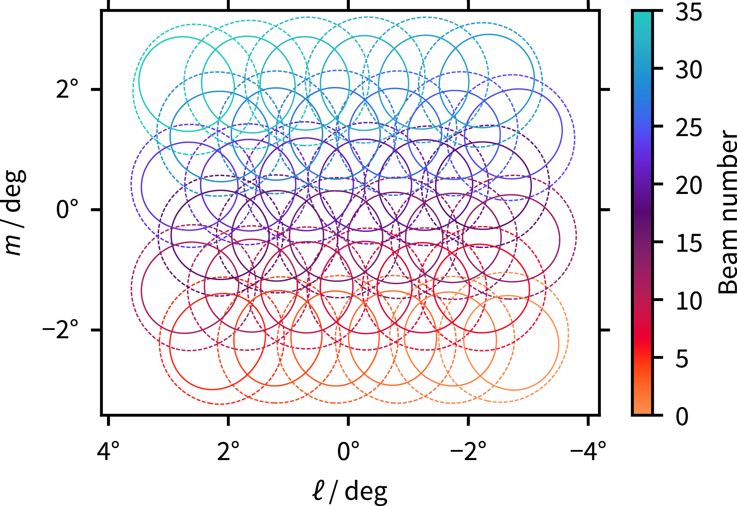
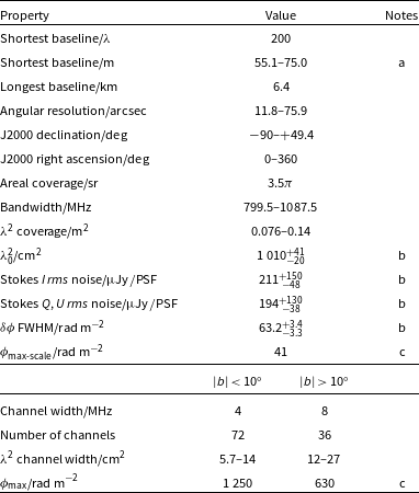
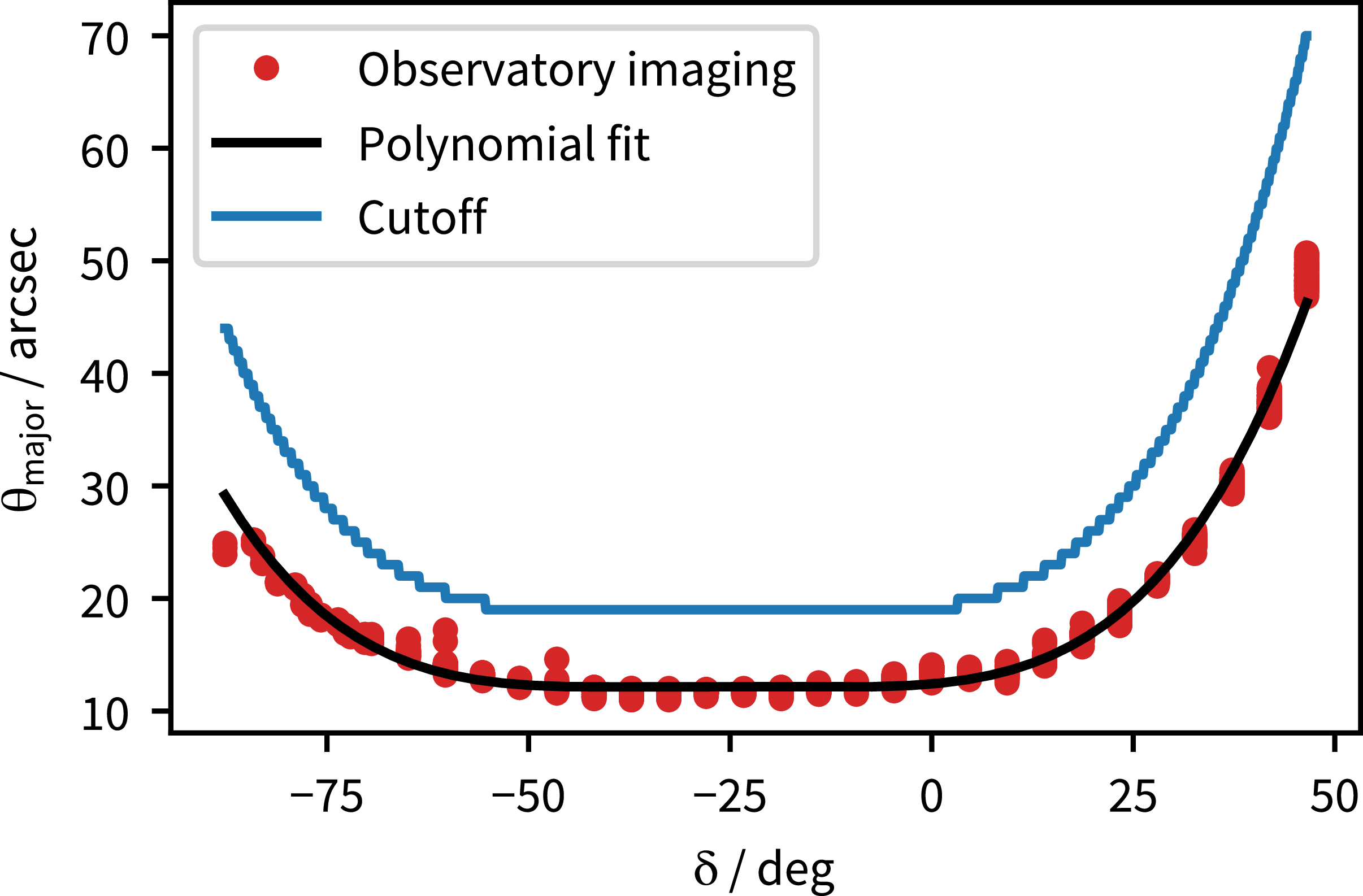
 θ
θ δ
δ θmajor
 θmajor=1.2×101+6.3×10⁻²δ+4.9×10⁻³δ2+1.4×10⁻⁴δ3+1.3×10⁻⁶δ4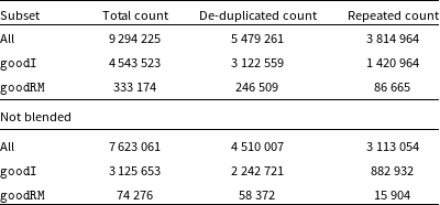
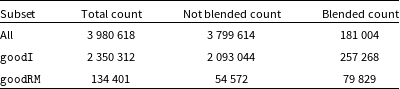
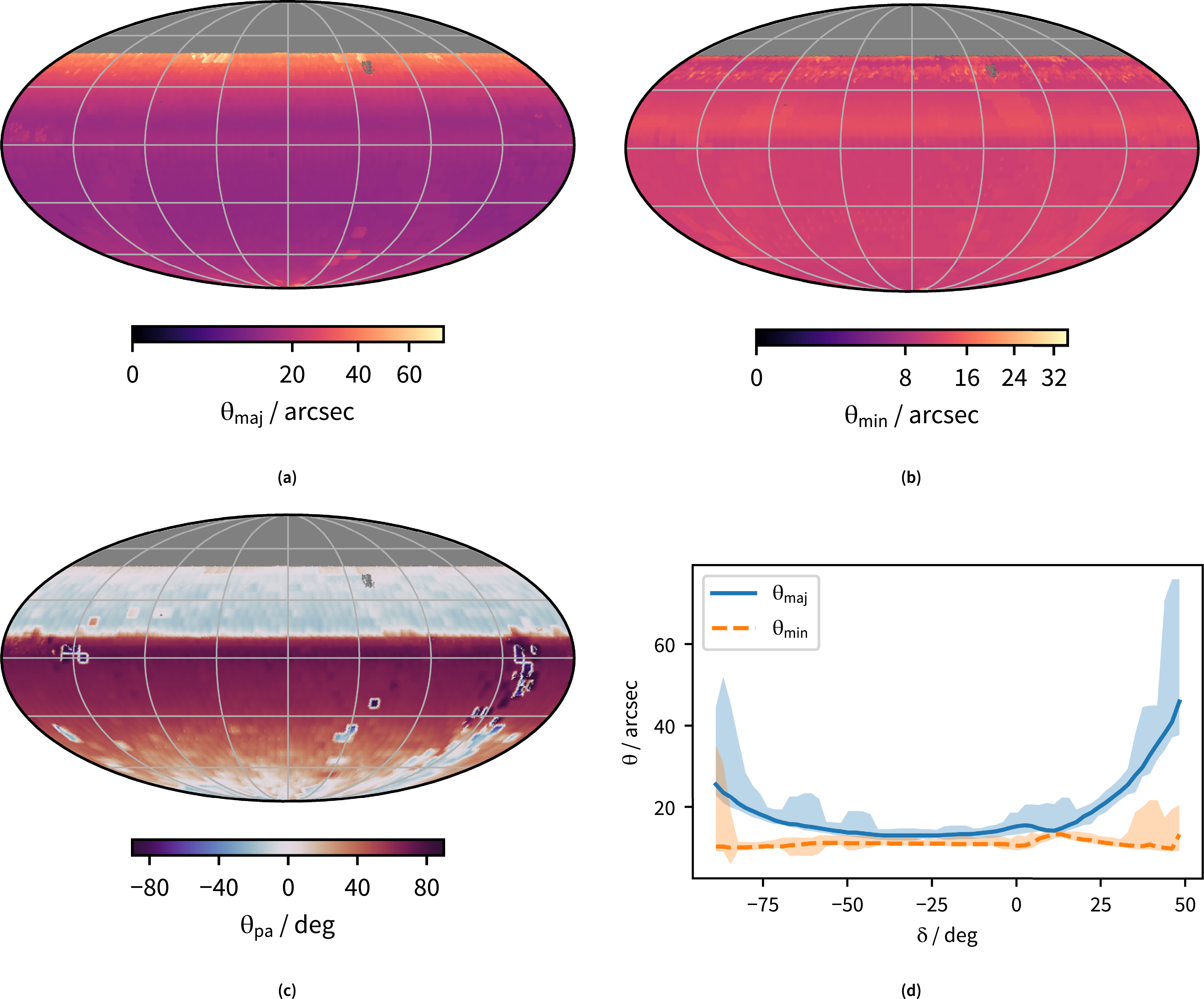
 θ
θ θmaj
θmaj δ
δ θmaj
θmaj θmin
θmin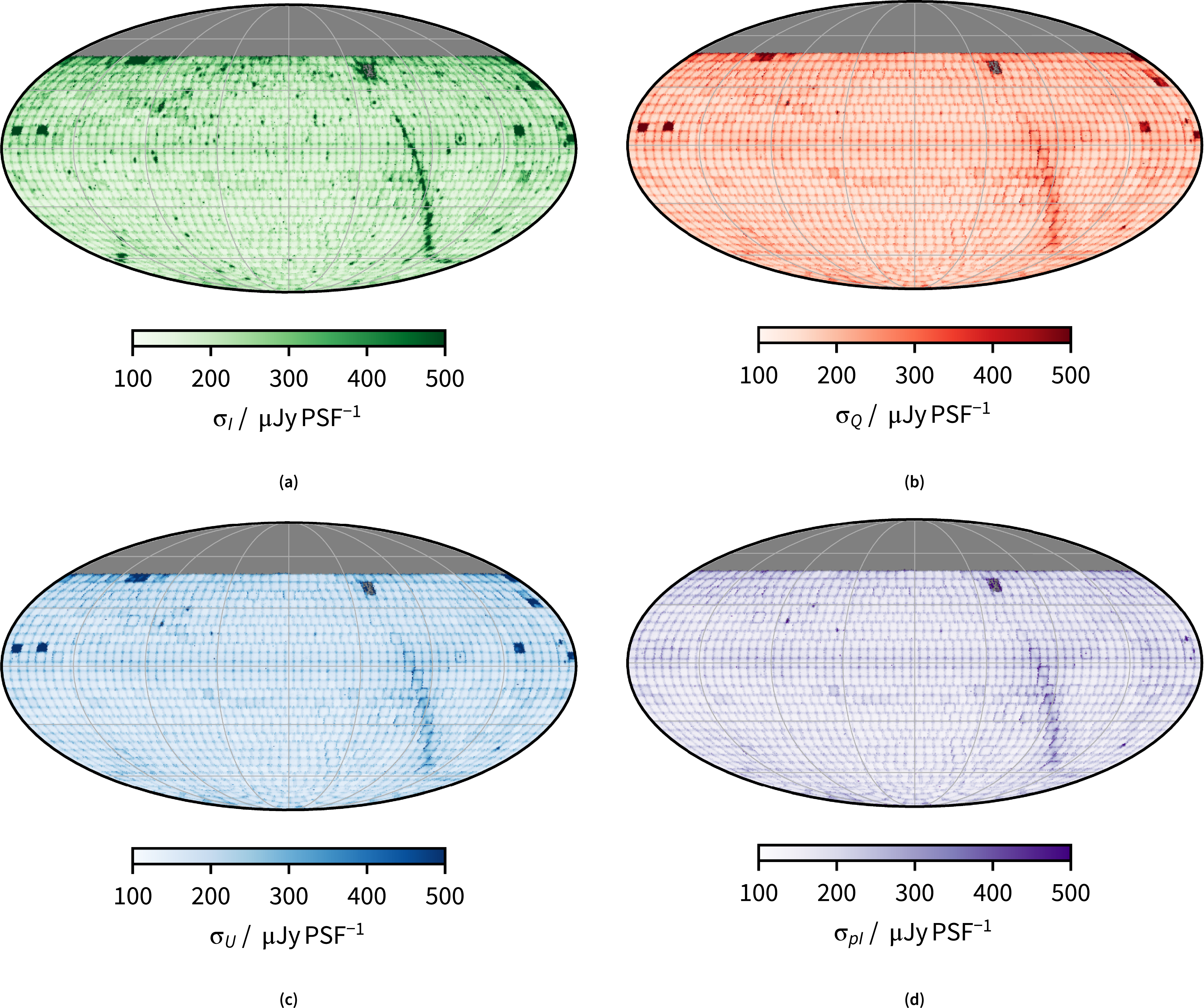
 σ
σ σpI
σpI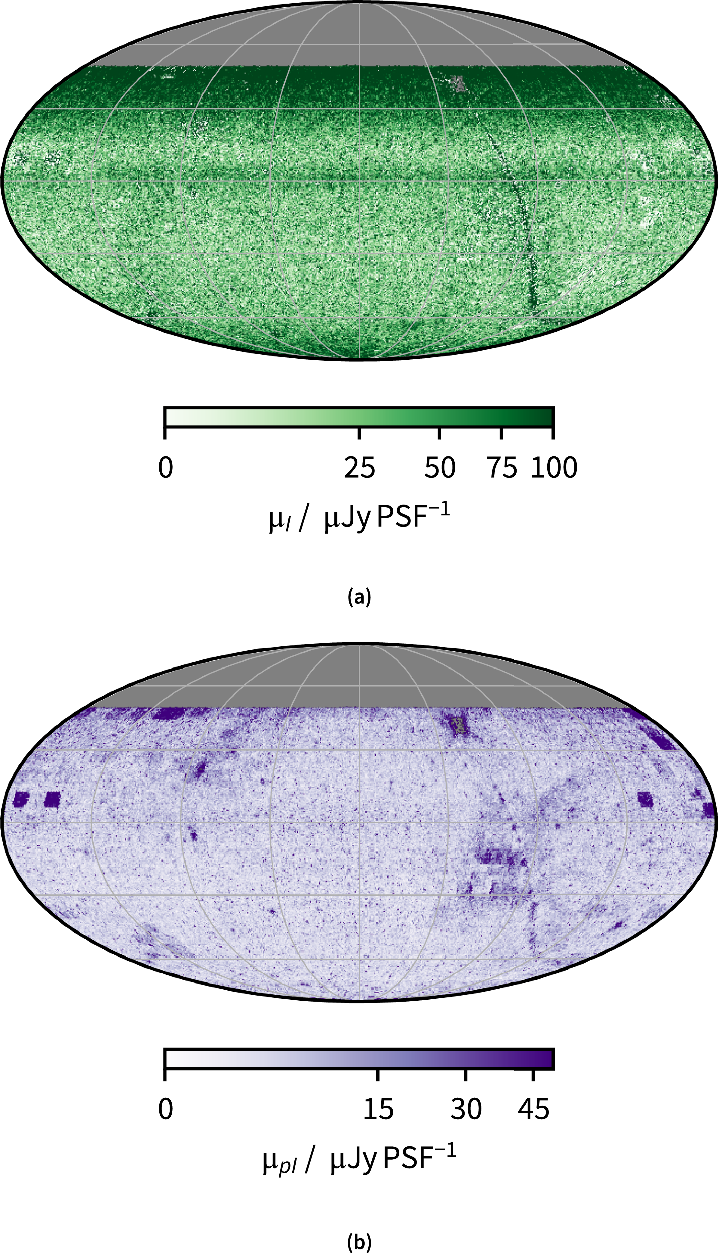
 μ
μ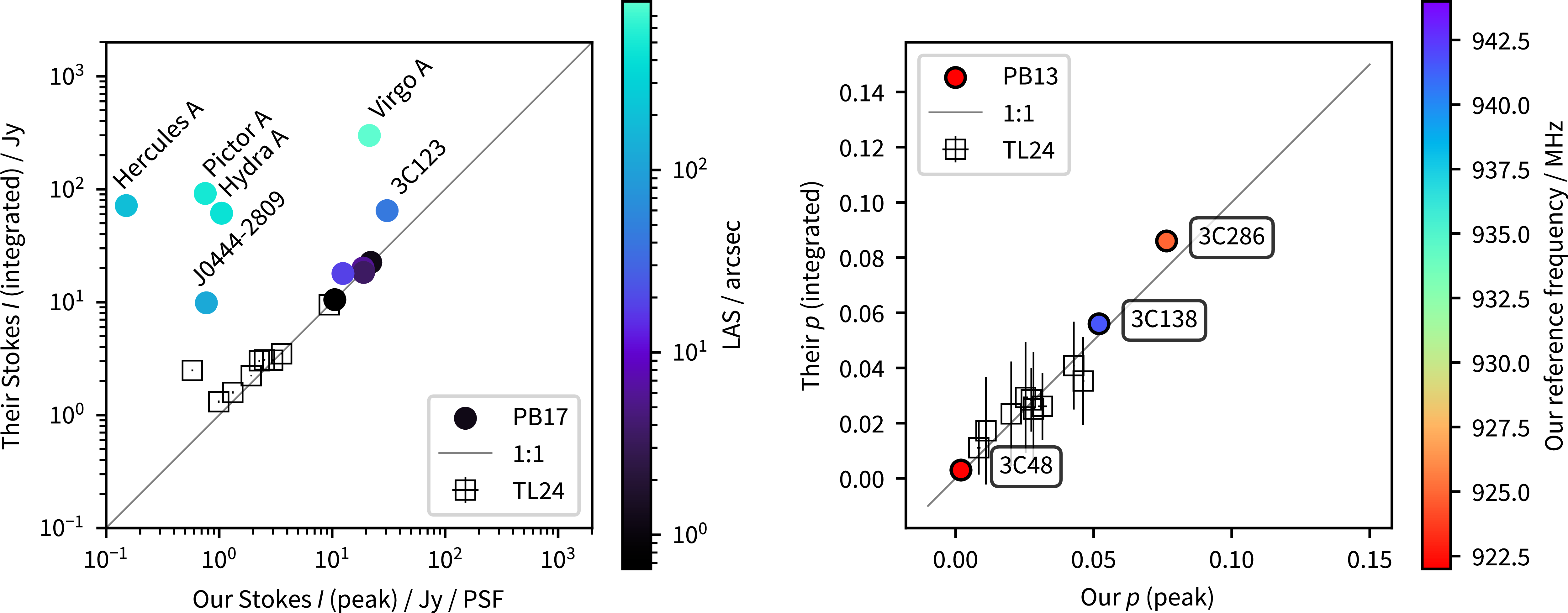
 LAS>20′′
 5σ
5σ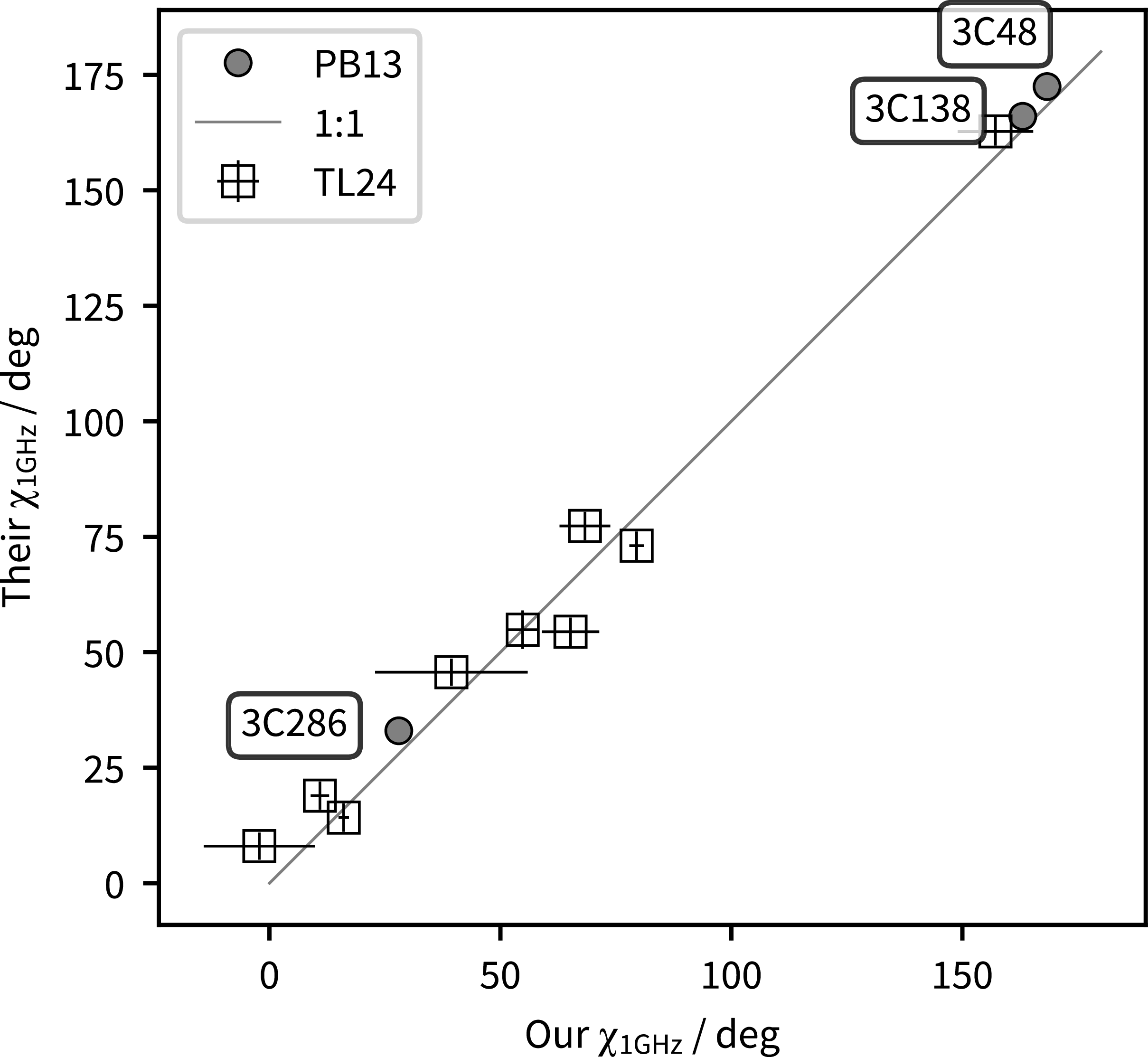
 χ
χ 5σ
5σ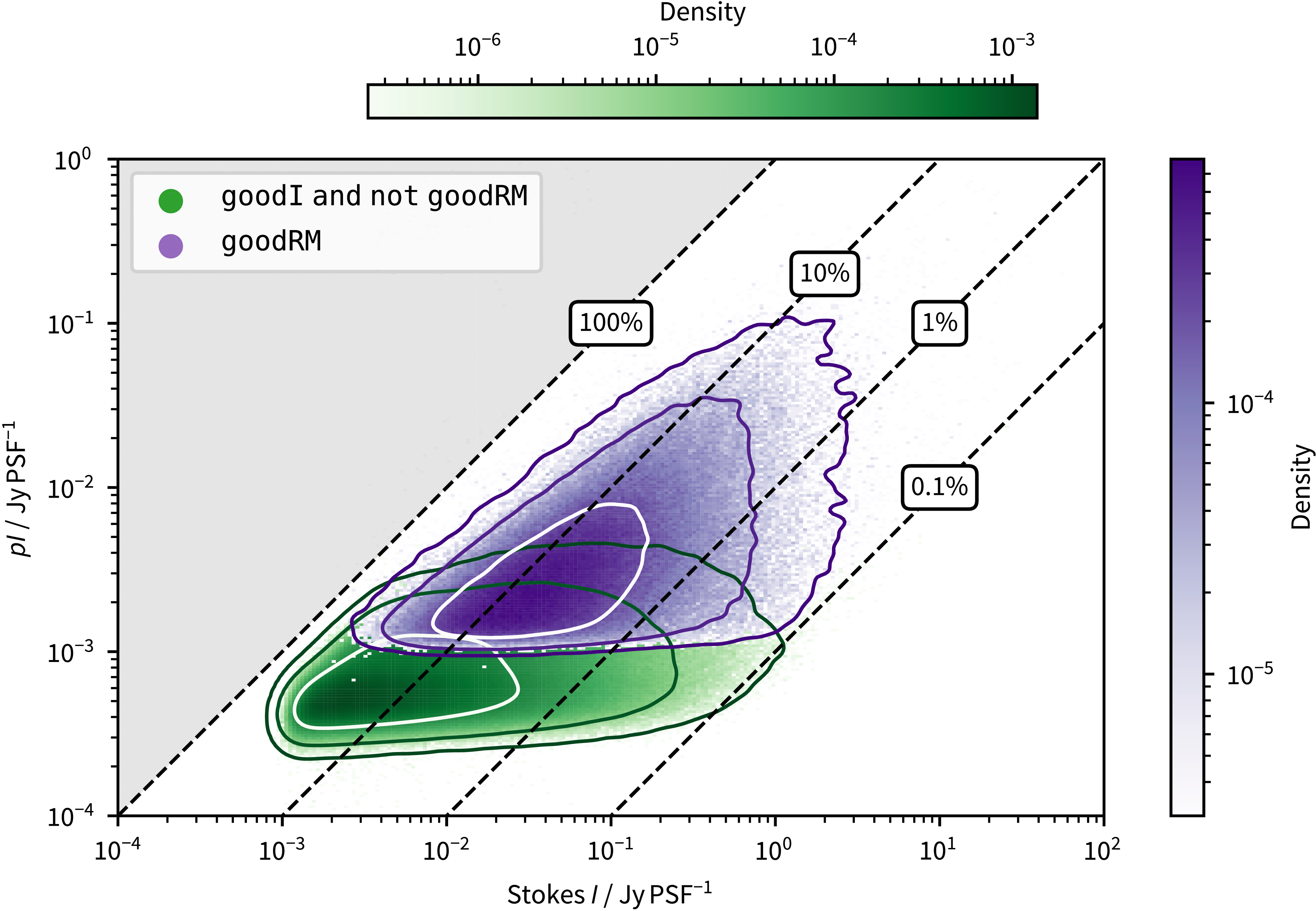
 16th
16th 50th
50th 84th
84th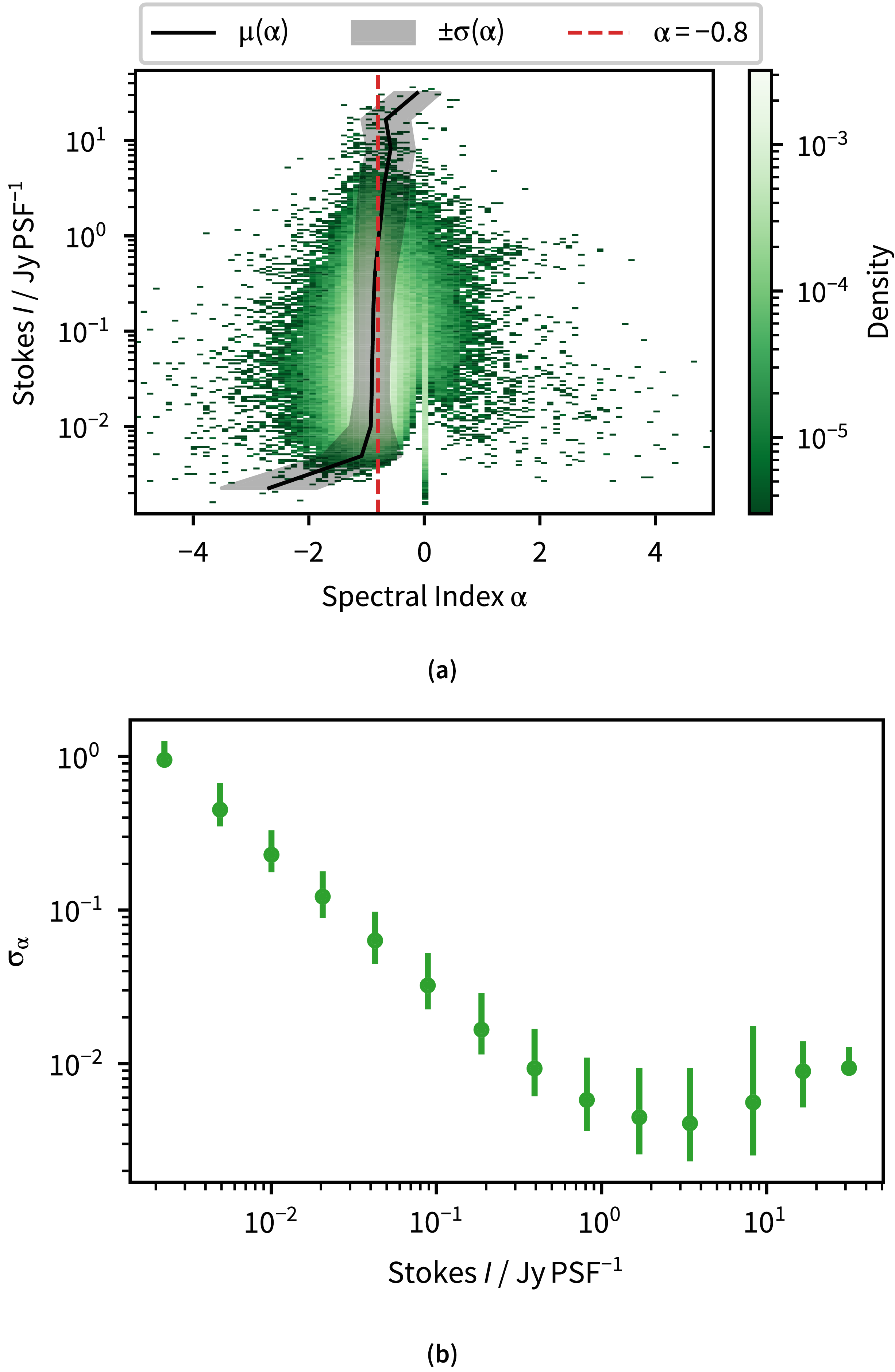
 α
α α
α −5≤α≤5
 μ
μ σ
σ α
α α=−0.8
 α=0
α=0 α=0
α=0 σα
σα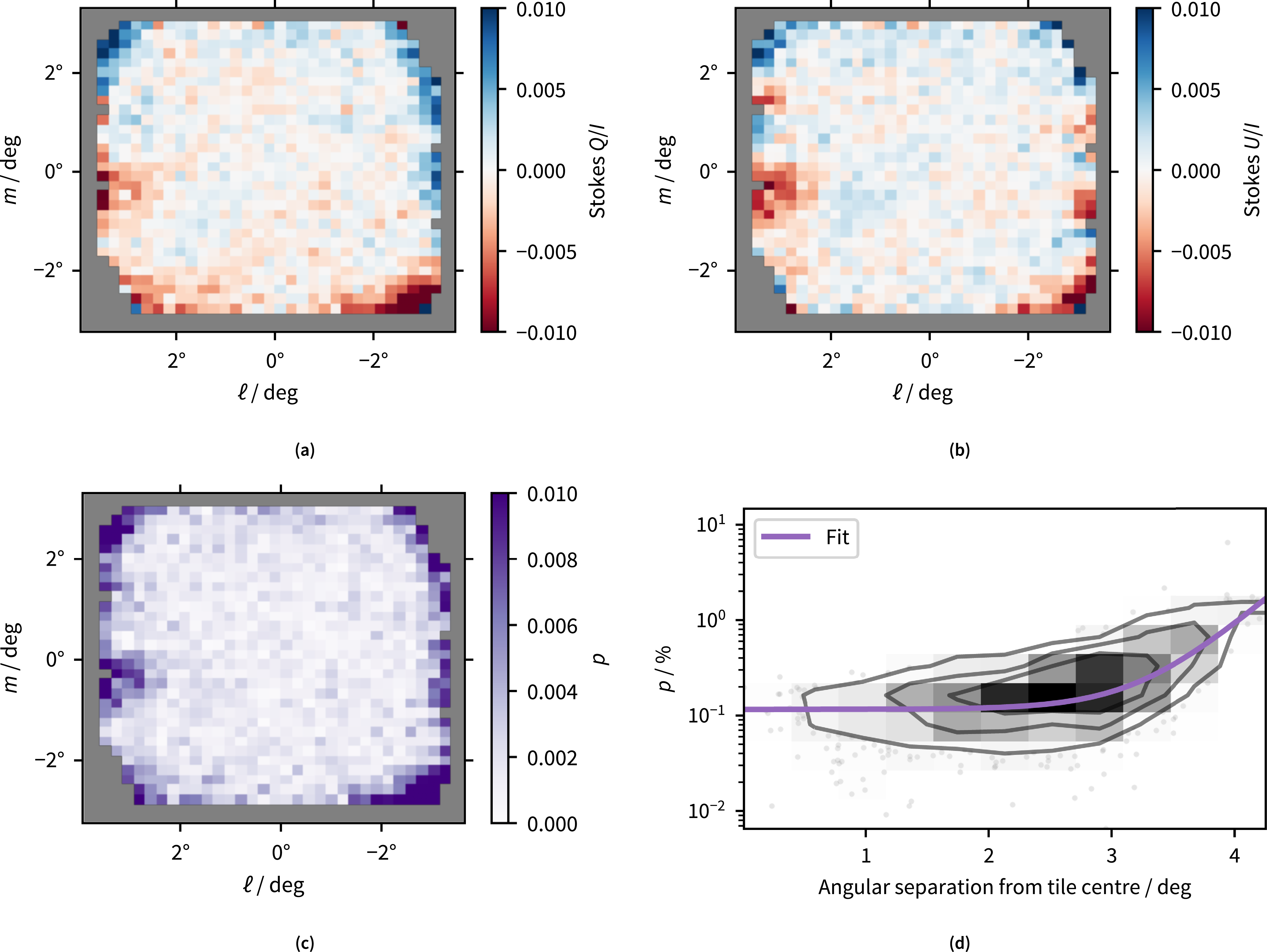
 aebϑ+c
 ϑ
ϑ a=2.7×10⁻⁷
 b=2.58
 c=1.16×10⁻³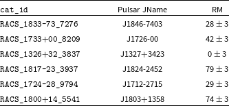
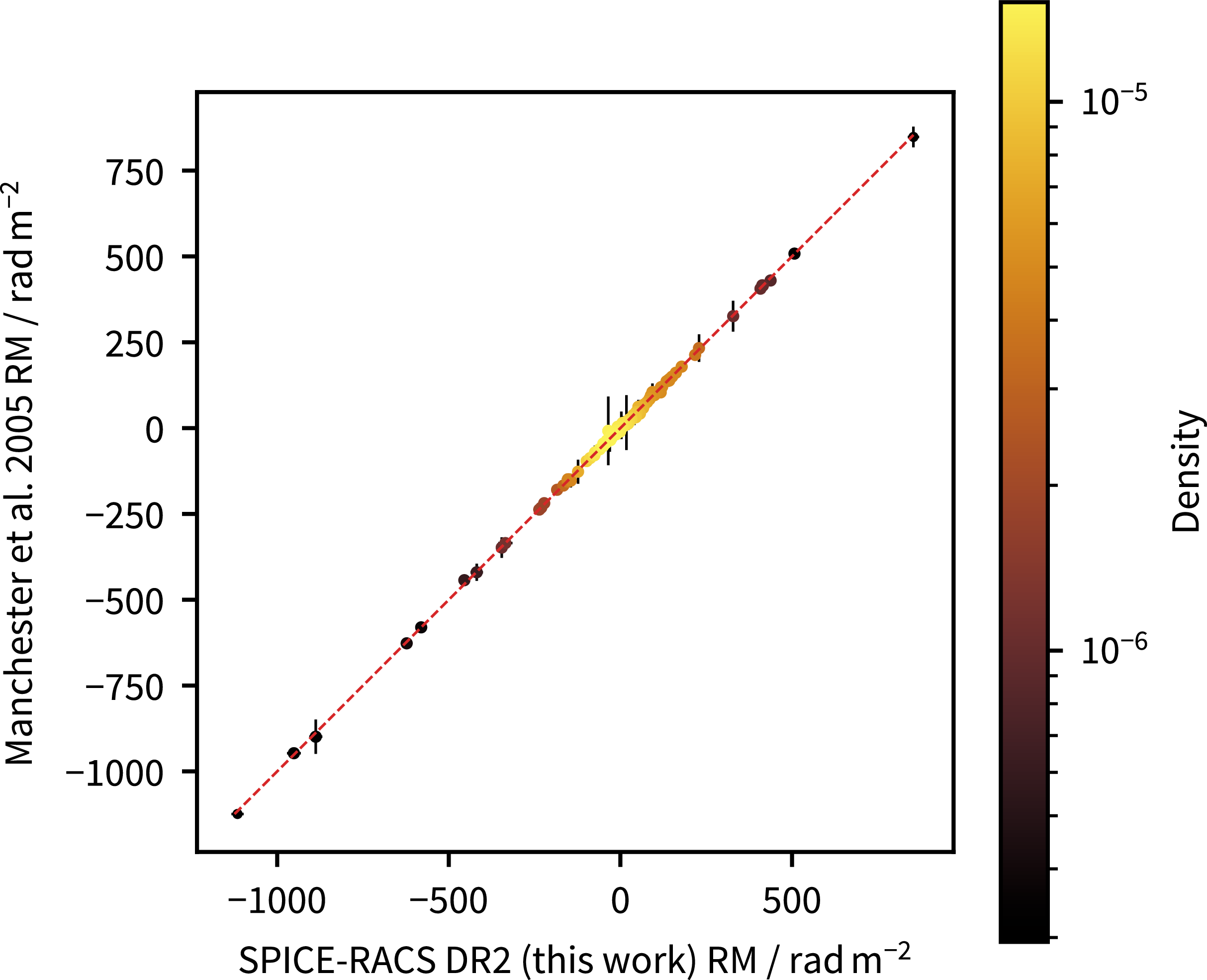
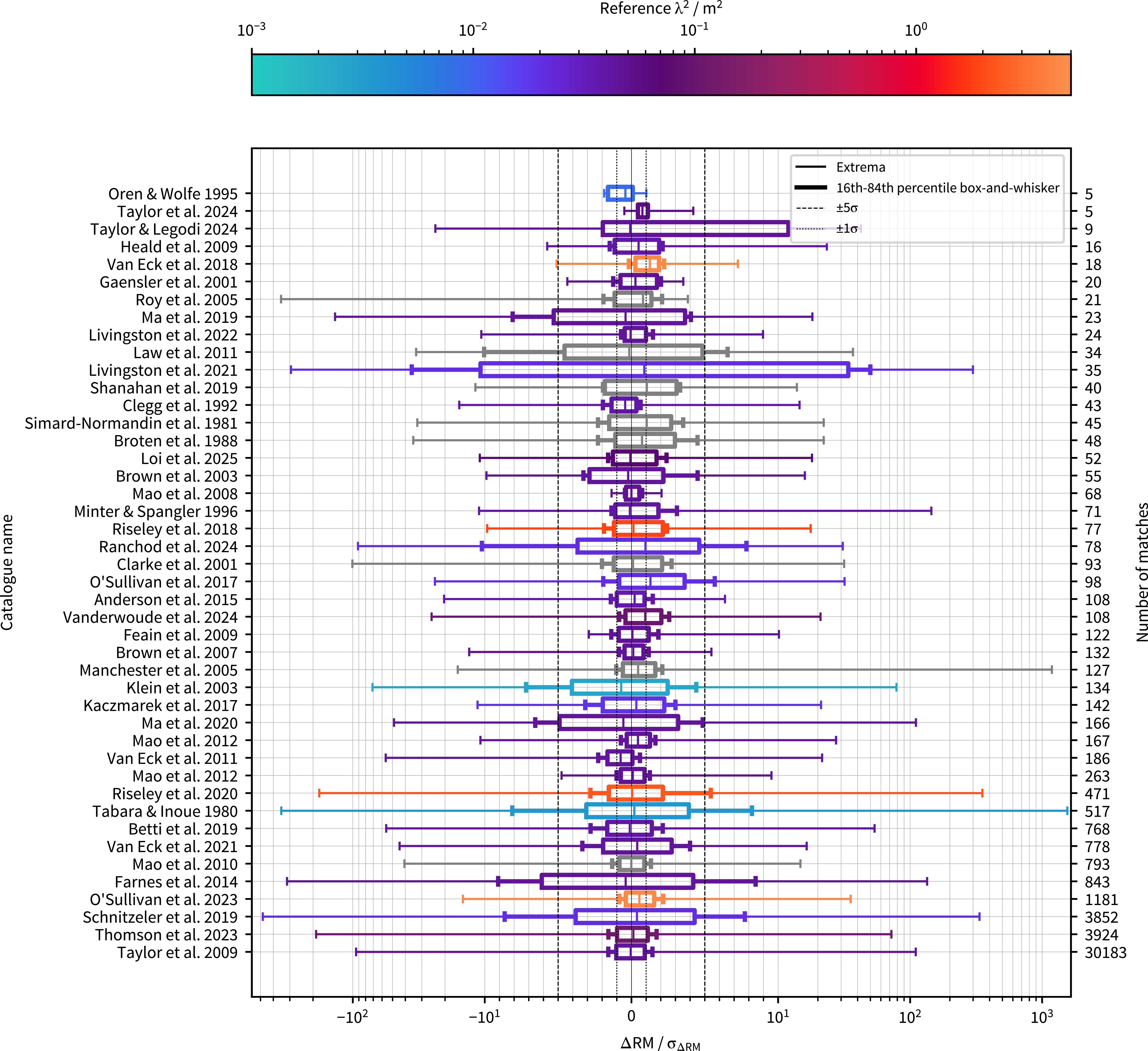
 ΔRM
ΔRM ΔRM
ΔRM σΔRM
σΔRM ΔRM/σΔRM
 ±1σ
±1σ ±5σ
±5σ ±1σ
±1σ λ2
λ2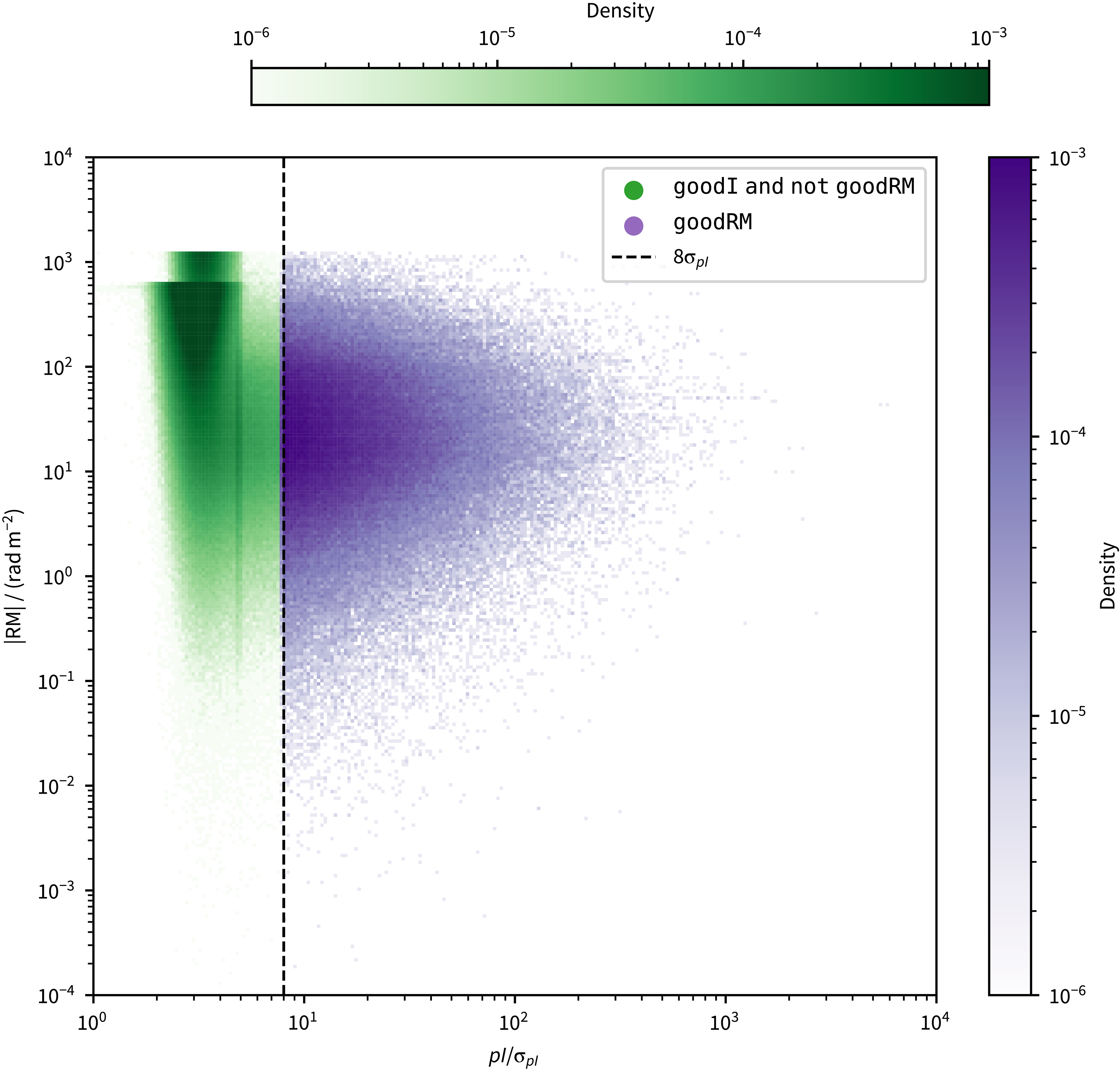
 |RM|
|RM| pI/σpI
 pI/σpI=8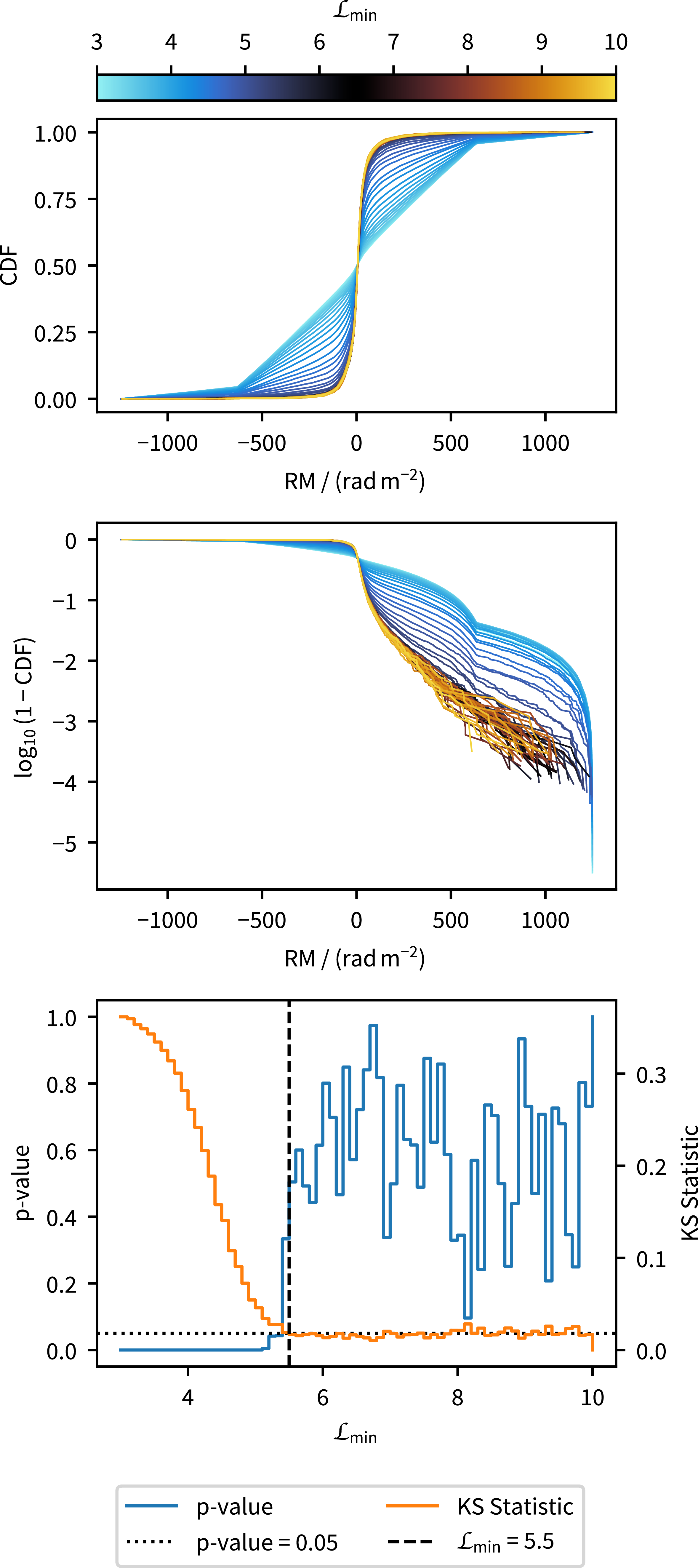
 L=pI/σpI
 Lmin
Lmin Lmin
Lmin Lmin
Lmin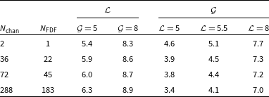
 Nchan
Nchan NFDF
NFDF L=pI/σpI
 G
G G
G L
L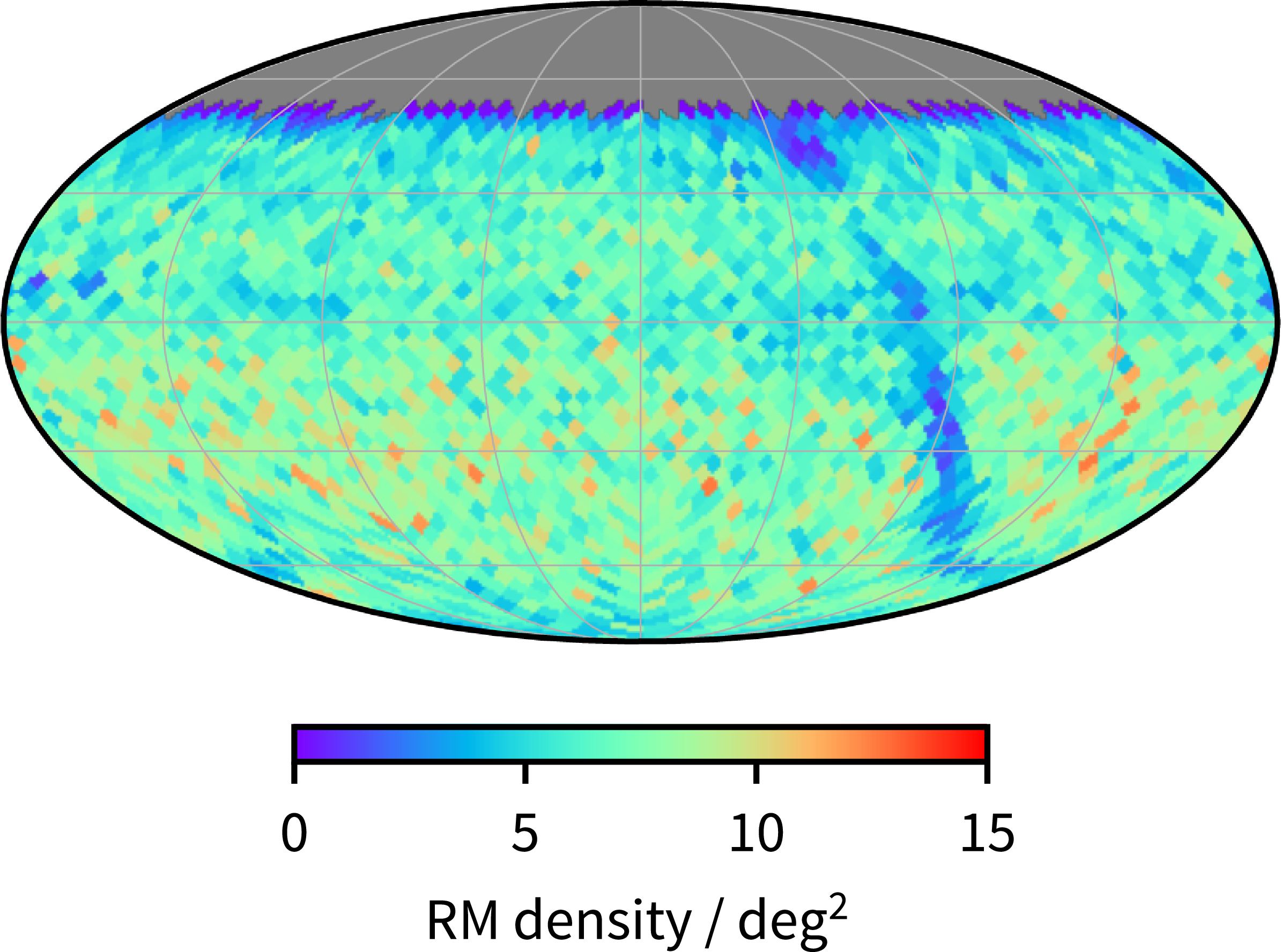
 Nside=16
 ∼220′
∼220′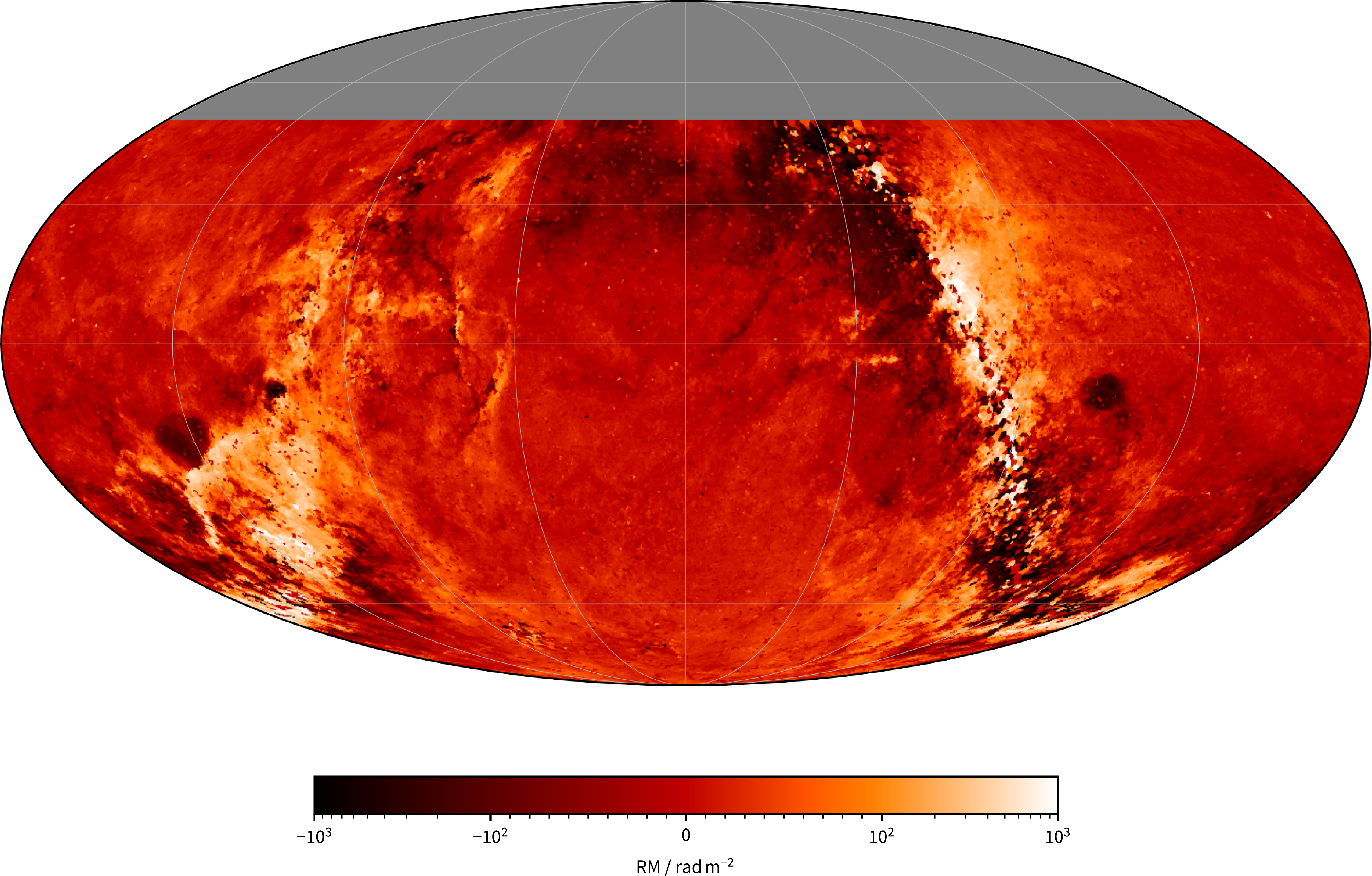
 |RM|≤100radm−2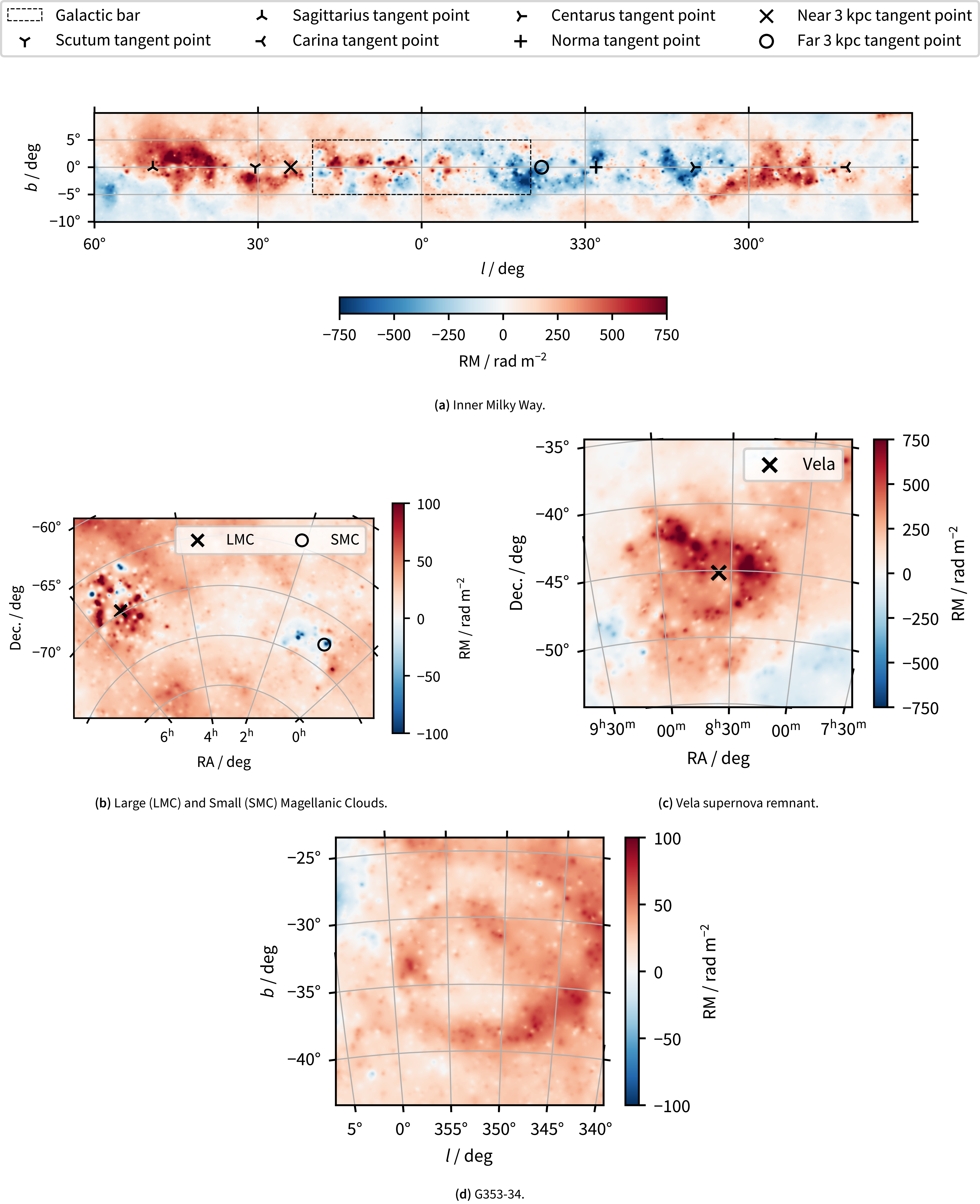
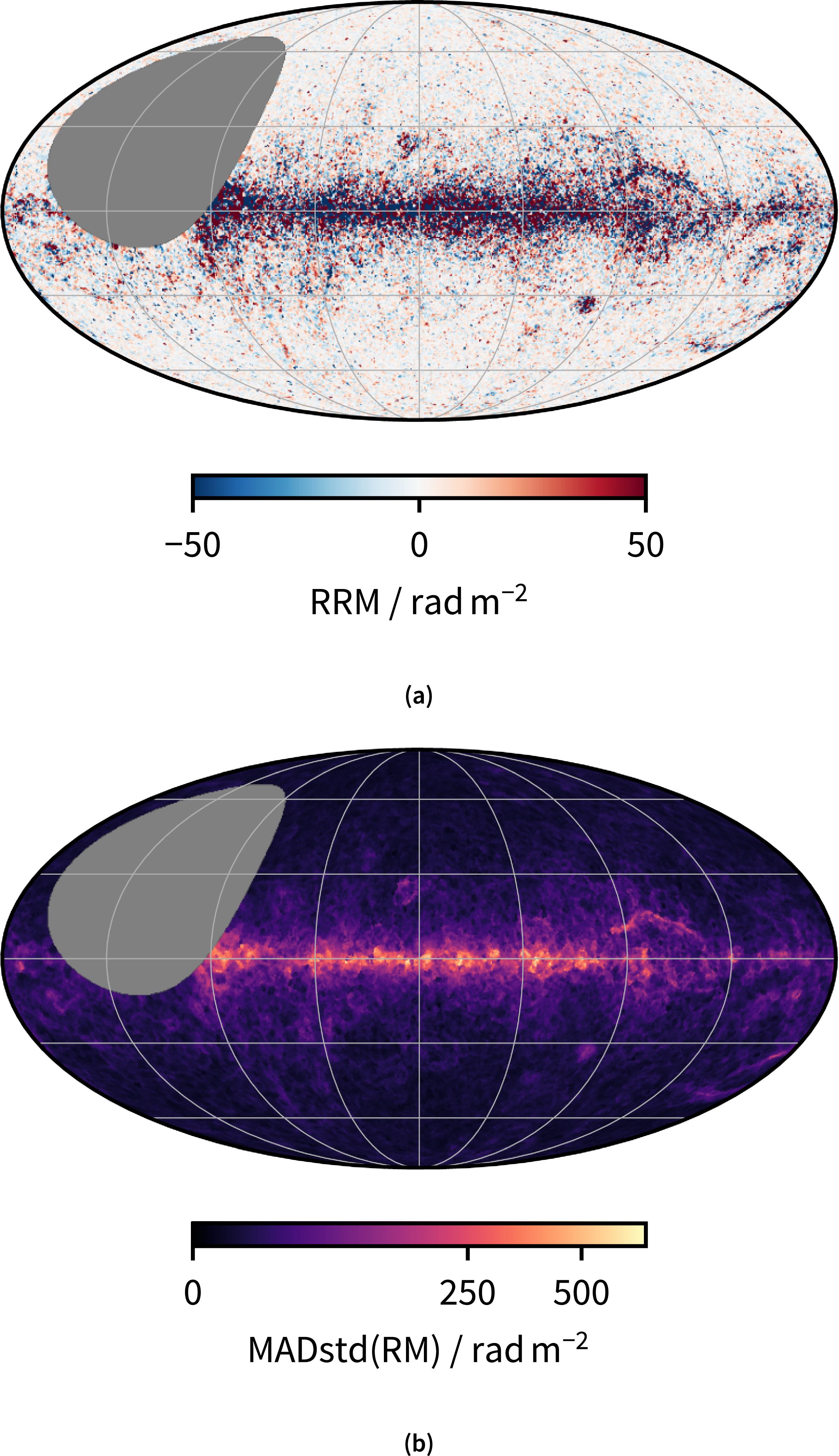
 l,b=(0∘,0∘)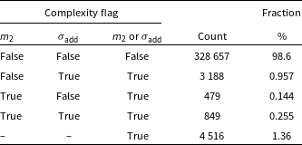
 m2
m2 σadd
σadd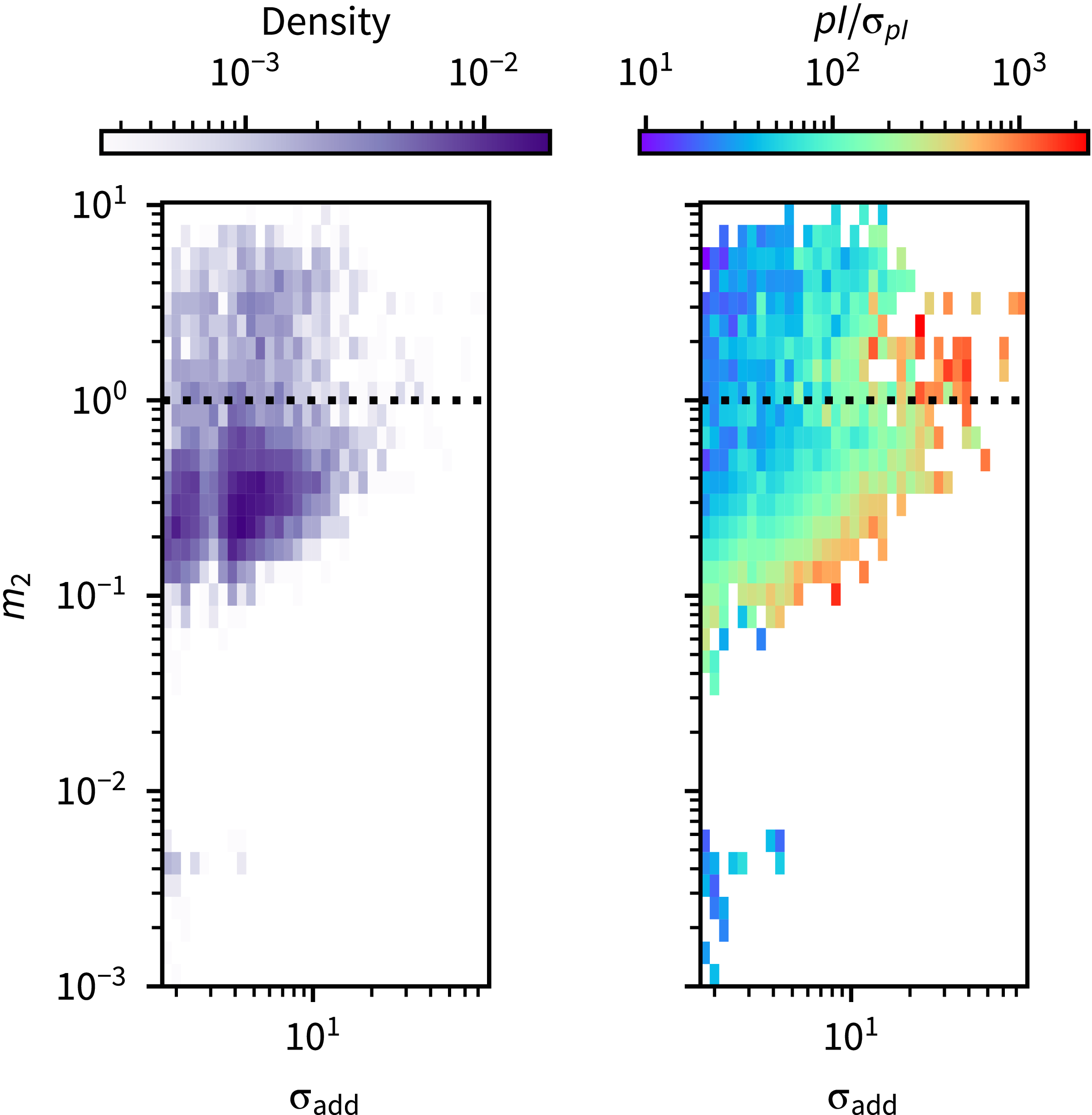
 m2
m2 σadd
σadd pI/σpI
 m2=1
m2=1 m2>1
m2>1 σadd
σadd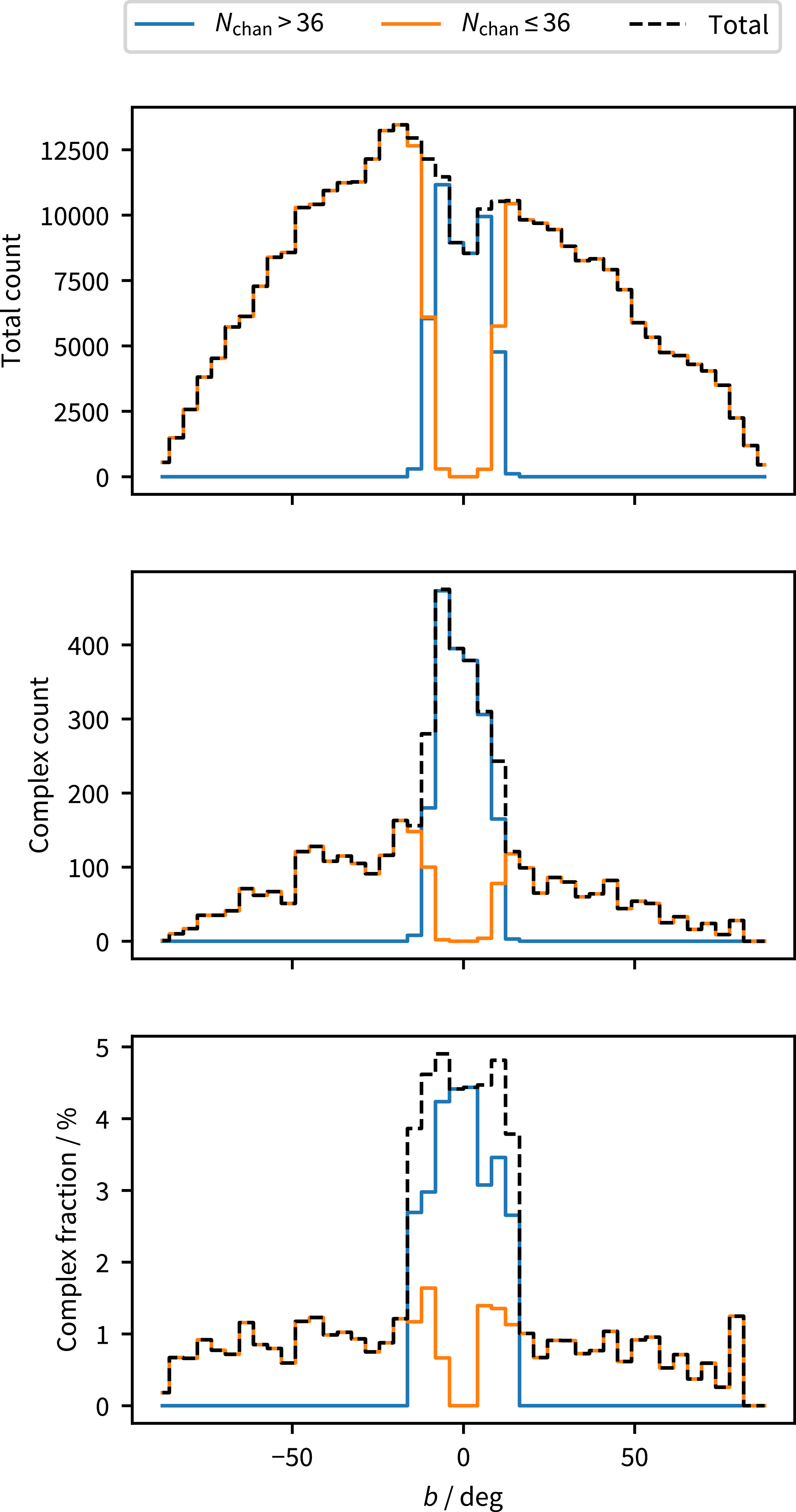
 Nchan
Nchan >36
>36 ≤36
≤36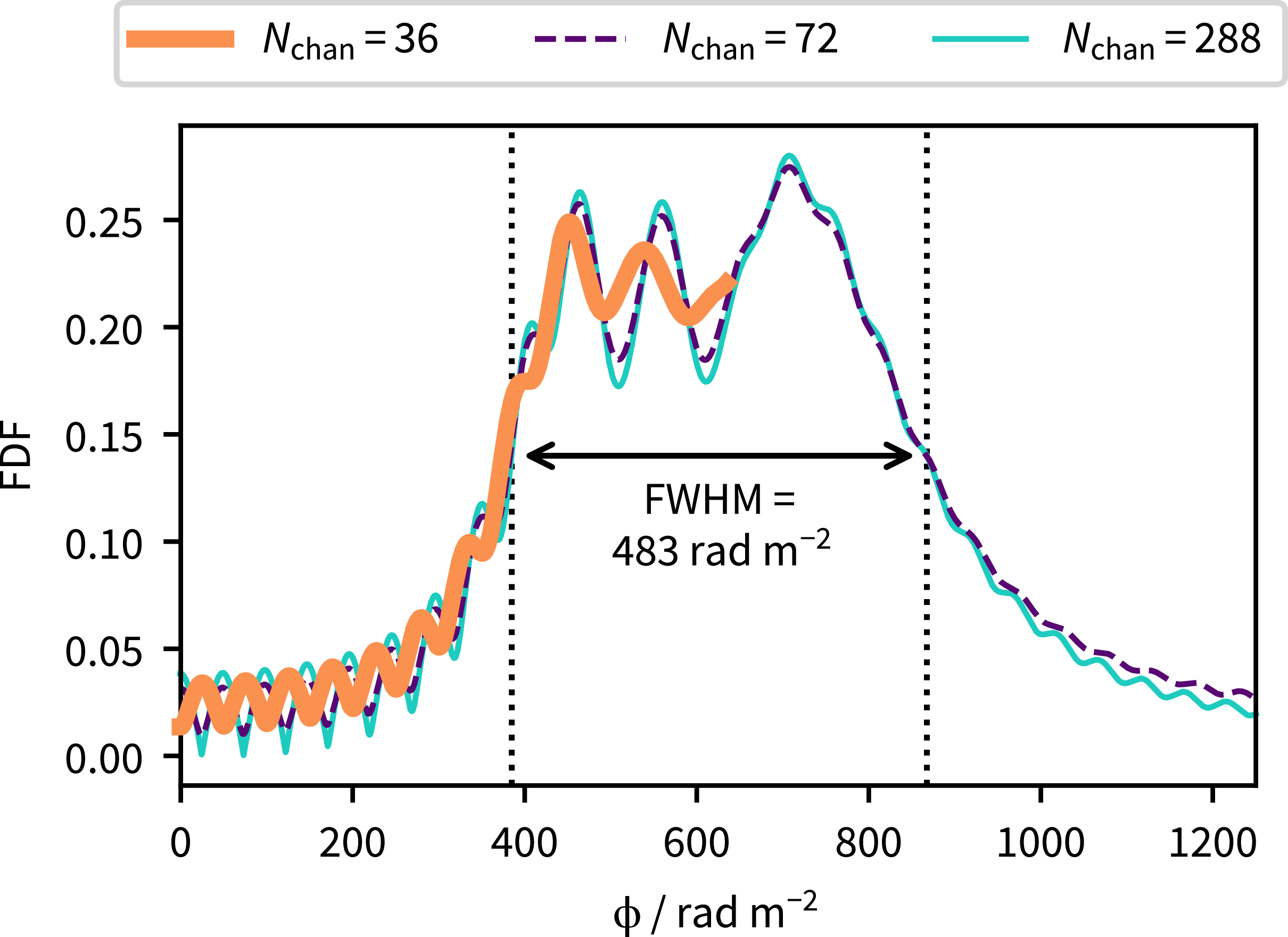
 Nchan
Nchan ϕ=0
ϕ=0 ϕ>0
ϕ>0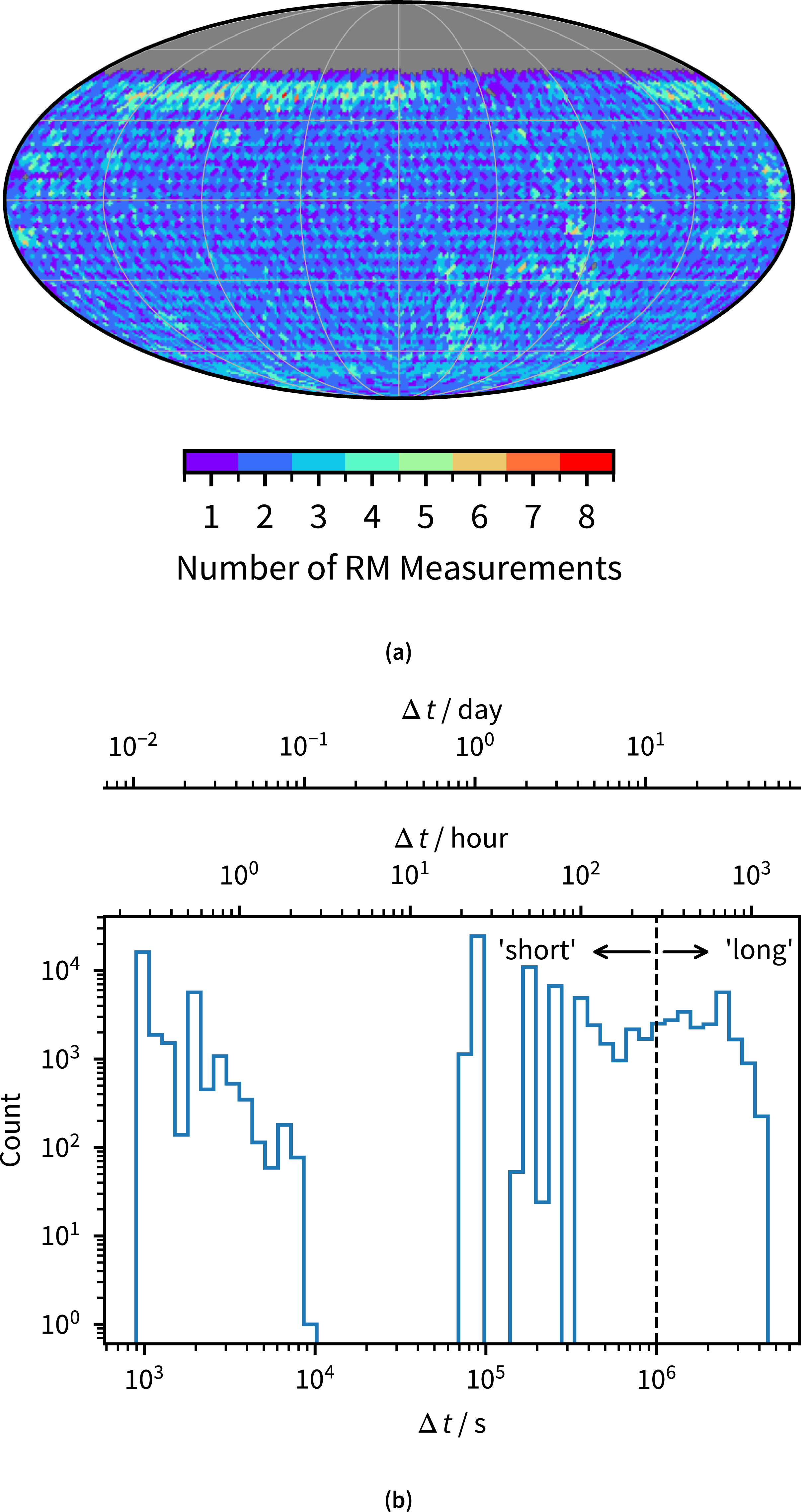
 Δt
Δt Δt
Δt 106
106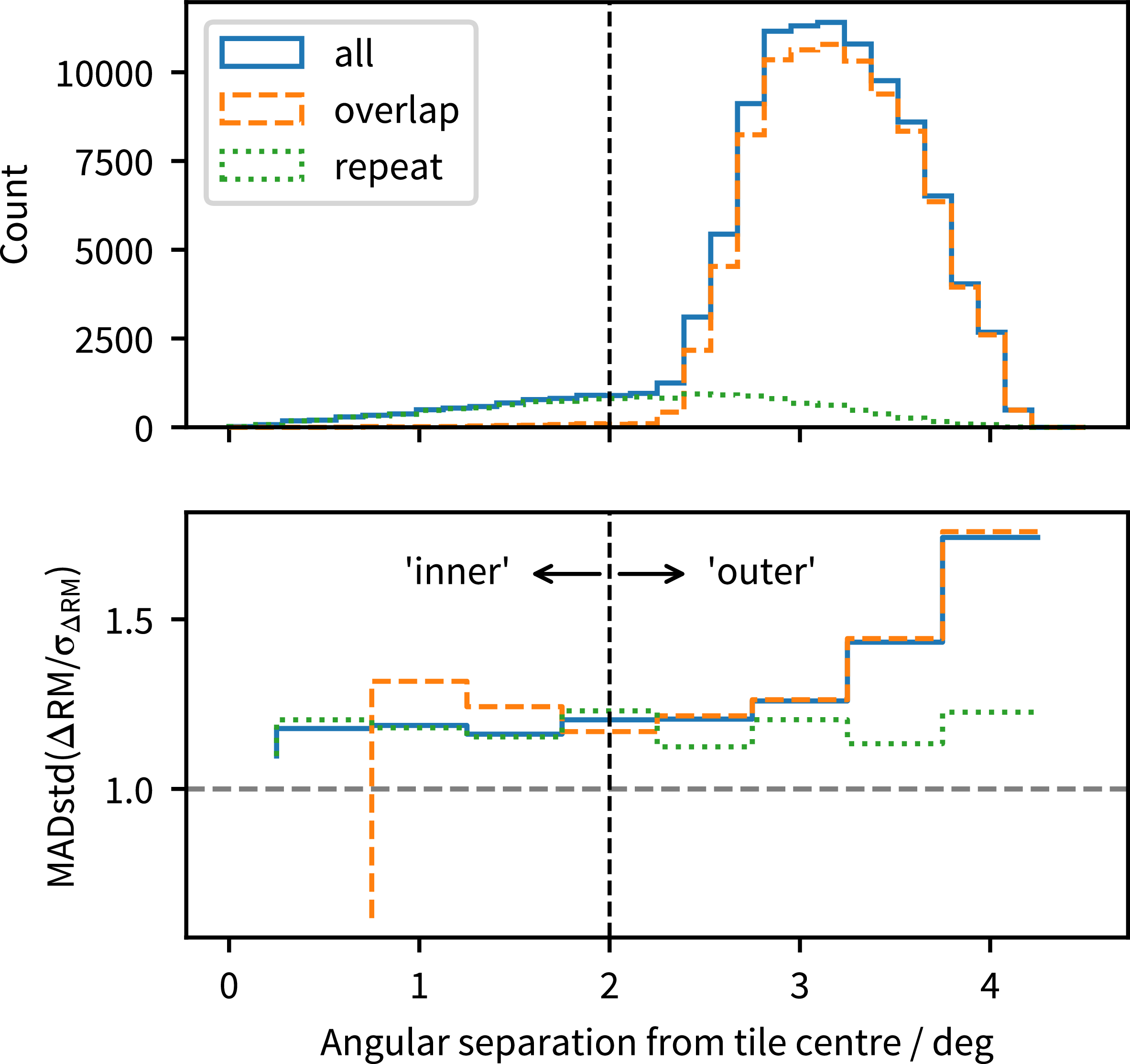
 2∘
2∘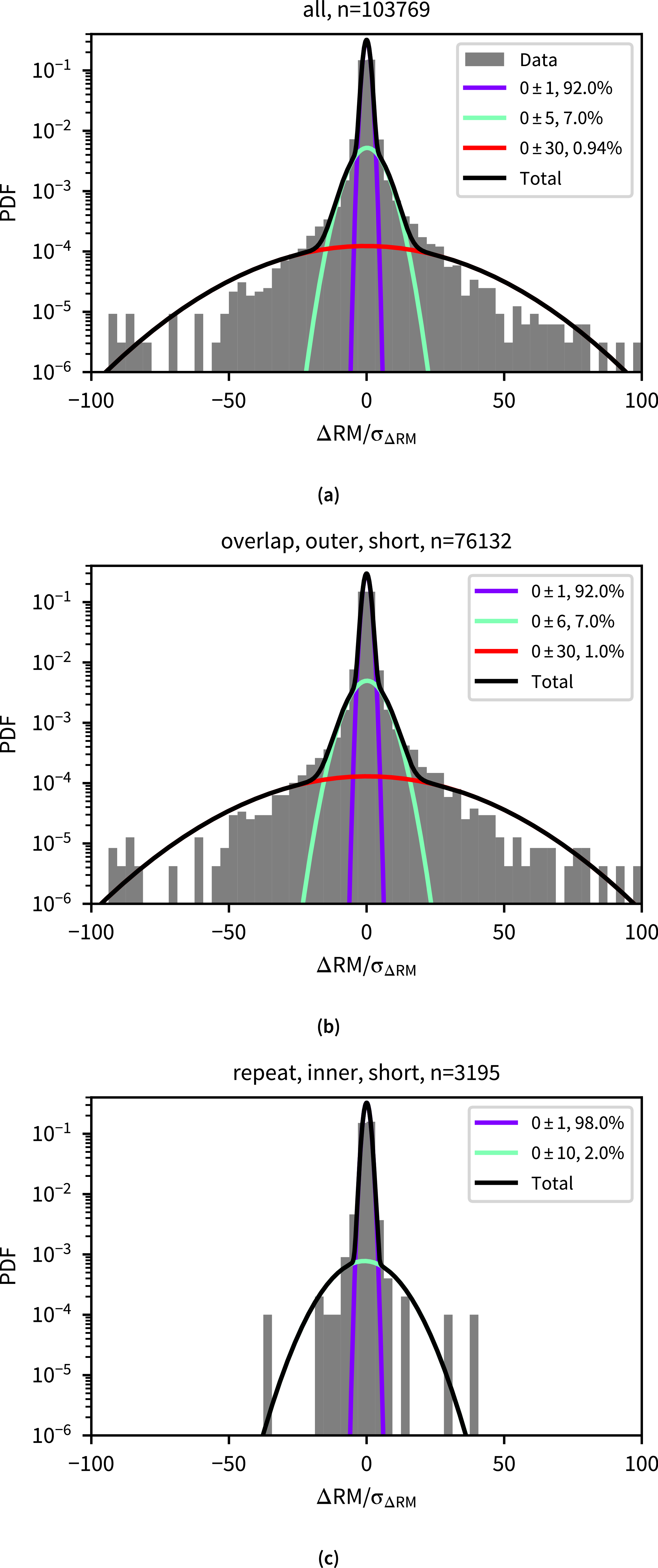
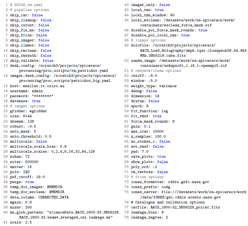
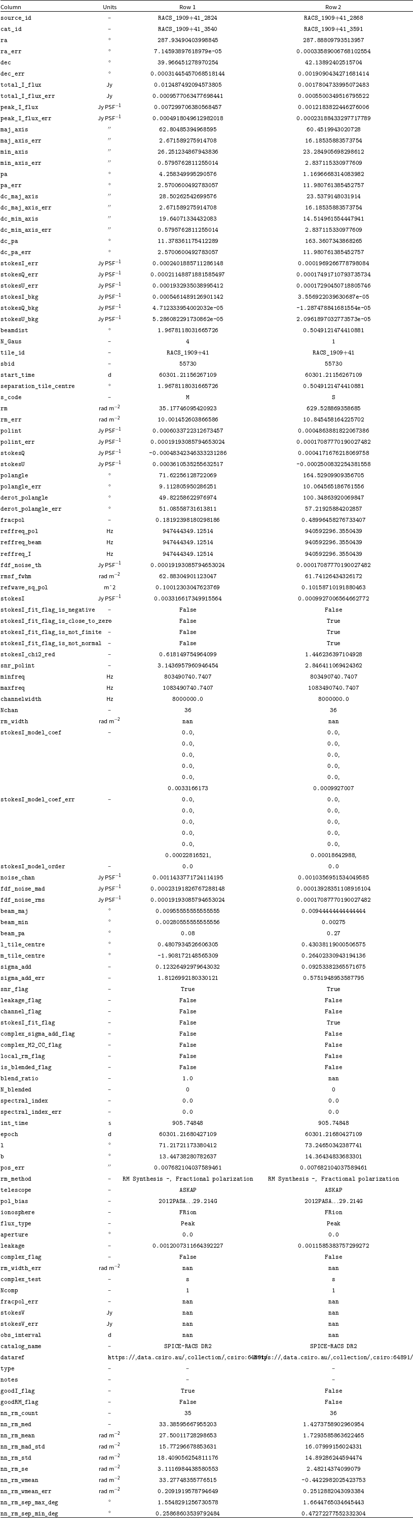
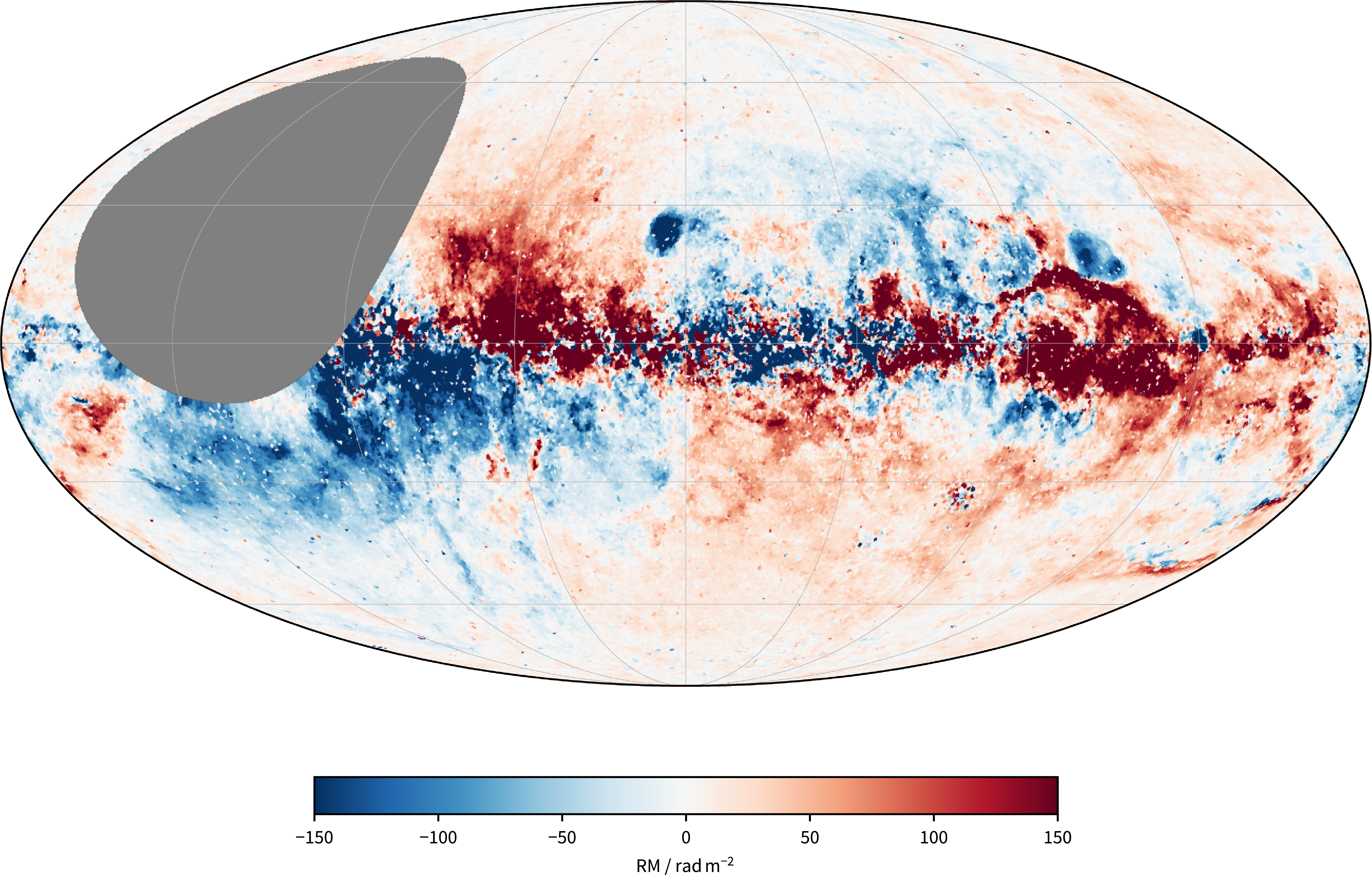

 Open access

