2. Thwaites method for laminar boundary layers

In this section, a brief summary of the method of Reference ThwaitesThwaites (1949) for approximating the momentum thickness of laminar boundary layers is provided. For thin boundary layers in an incompressible flow, the von Kármán integral equation (White Reference White2008) is written as

(2.1)\begin{equation} \frac{{\rm d} \theta}{{\rm d} s} + (2 + H) \frac{\theta}{U_e} \frac{{\rm d} U_e}{{\rm d} s} = \frac{C_f}{2}, \end{equation}

where in the $n$–$s$ coordinate system, $s$ is the streamwise coordinate, and $n$ is the wall-normal coordinate. Here $\delta ^{*}$ and $\theta$ are the boundary layer's displacement and momentum thickness lengths, respectively, and $H = \delta ^*/\theta$ is the shape factor. The following relations also hold under the thin boundary layer approximation:

(2.2)\begin{equation} \nu \left.\frac{\partial^2 U}{\partial n^2} \right|_{n = 0} = \frac{1}{\rho } \frac{{\rm d} P_e}{{\rm d} s} = {-} U_e \frac{{\rm d} U_e}{{\rm d} s}, \end{equation}

where $P_e$ and $U_e$ are the values of the pressure and the streamwise velocity at the edge of the boundary layer, and $n=0$ refers to the wall. This relation invokes ${\rm d}P/{\rm d}n \rightarrow 0$ within the boundary layer under the thin boundary layer approximation. Thus, the ${\rm d}P/{\rm d}s$ at the edge of the boundary layer (${\rm d}P_e/{\rm d}s$) is considered to be approximately the same as that on the wall ($n=0$). Using these relations, (2.1) is rearranged as

(2.3)\begin{equation} 2 Re_{\theta} \frac{{\rm d} \theta}{{\rm d} s} = 2((2 + H) m + \chi) = L, \end{equation}

where $m$ is the Holstein–Bohlen pressure gradient parameter, $m = ({\theta ^2}/{U_e}) ({\partial ^2 U }/{\partial n^2}) |_{n=0}$ and $\chi = ({\theta }/{U_e}) ({\partial U}/{\partial n}) |_{n=0}$. It should be noted that in deriving (2.3), the assumption of a laminar flow has not yet been invoked. For laminar boundary layers, however, Thwaites further postulated that $L = L(m)$, or that the effect of the pressure gradient primarily determines the growth rate of a laminar boundary layer. Specifically, the linear fit proposed in Thwaites’ original work is

(2.4)\begin{equation} L \approx L(m)^{Thwaites} \approx 0.45 + 6m. \end{equation}

Rearranging the model fit, an approximate closed-form expression of the momentum thickness can be written as

(2.5)\begin{equation} \theta^2(s) \approx 0.45 \frac{\nu}{U^6_e} \int^s_0 U^5_e(r) \,{\rm d}r. \end{equation}

Further, Thwaites fitted experimental data to suggest that a laminar flow may separate when $m \approx 0.09$. Other similar empirical thresholds have been proposed by Reference StratfordStratford (1959) and by Reference Curle and SkanCurle & Skan (1957). More details can be found in Reference HortonHorton (1968). Reference Curle and SkanCurle & Skan (1957), and later Reference Dey and NarasimhaDey & Narasimha (1990) suggested slightly different model coefficients that resulted in a better agreement with the Blasius and Falkner–Skan type solutions.

3. Methods for turbulent flows

In this section, two commonly known methods for predicting the momentum thickness of a turbulent boundary layer in the presence of a pressure gradient are described.

3.1 Head's integral momentum equation

Similar to Thwaites’ method for laminar boundary layers, Reference HeadHead (1958) and Reference Head and PatelHead & Patel (1968) proposed an integral momentum equation-based approach for predicting the growth of the momentum thickness and the location of a separation point for turbulent boundary layers. The original work (Reference HeadHead 1958) was developed as follows. Using the correlation for the skin-friction (from Reference Ludwieg and TillmannLudwieg & Tillmann (1950)) and an auxiliary relation between the shape factor ($H$) and the entrainment factor ($H_1$), a system of two differential equations governing the growth of the momentum thickness is given as

(3.1)\begin{gather} \frac{{\rm d} \theta}{{\rm d} s} + (2 + H) \frac{\theta}{U_e} \frac{{\rm d} U_e}{{\rm d} s} = \frac{C_f}{2}, \end{gather}

(3.2)\begin{gather}C_f = 0.246 (10^{{-}0.678 H}) Re^{{-}0.268}_{\theta}, \end{gather}

with the shape factor ($H$) and the entrainment factor ($H_1$) related as

(3.3)\begin{equation} \frac{1}{U_e} \frac{{\rm d}}{{\rm d}s} (U_e \theta H_1) = 0.0299 (H_1 - 3.0)^{{-}0.6169}, \end{equation}

and $H_1 = 0.8234(H-1.1)^{-1.287}$ for $H \leq 1.6$, and $H_1 = 1.55(H-0.6778)^{-3.064} + 3.3$ otherwise. Reference HeadHead (1958) and the further developments in Reference Head and PatelHead & Patel (1968) showed that the method can reasonably predict the growth of the momentum thickness for two-dimensional, non-equilibrium boundary layers. It is remarked that compared with Thwaites’ method (which requires one empirical correlation), this approach requires additional correlations ((3.2)–(3.3) and $H_1 = f(H)$). For a comprehensive review, the reader is referred to Reference Cebeci and BradshawCebeci & Bradshaw (1977).

3.2 Drela's method

The method of Reference Giles and DrelaGiles & Drela (1987), Reference Drela and GilesDrela & Giles (1987) and Reference DrelaDrela (1989) has also been used to account for the viscous effects over airfoil flows. This formulation combines a potential flow panel method and an integral approach within the boundary layer. The viscous solution requires a correlation for the skin friction in terms of the shape factor to close the exact integral momentum equations. For an incompressible boundary layer, the invoked correlation from Reference SwaffordSwafford (1983) is given as

(3.4)\begin{equation} C_f = 0.3\,{\rm e}^{{-}1.33 H} [\log_{10}(Re_\theta)]^{{-}1.74-0.31 H} + 0.00011 \left[\tanh \left( 4 - \frac{H}{0.875} \right) - 1 \right] \end{equation}

and a nonlinear system is solved to determine $H$ as follows. When $H < H_0$,

(3.5)\begin{equation} H = 1.505 + \frac{4}{Re_\theta} + \left(0.165-\frac{1.6}{Re^{0.5}_\theta} \right) \frac{ (H_0 - H)^{1.6}}{H}, \end{equation}

otherwise

(3.6)\begin{equation} H = 1.505 + \frac{4}{Re_\theta} + (H-H_0)^2 \left[ \frac{0.04}{H} + \frac{0.007 \log (Re_\theta )}{(H-H_0 + 4/\log (Re_\theta))^2 }\right], \end{equation}

where $H_0 = 4$ when $Re_\theta < 400$ or else $H_0 = 3 + 400/Re_\theta$.

Both these approaches differ significantly from Thwaites’ method in that the terms of the integral momentum boundary layer equation relating to the shape factor, $H$, and skin friction coefficient, $C_f$, are explicitly modelled. The present method described below attempts to make a direct extension of the Thwaites’ transformation, without explicitly invoking a correlation for $C_f$, Reynolds number, $Re_\theta$, and the shape factor, $H$.

4. Extension of Thwaites method to turbulent flows

In this section, we develop the proposed extension of Thwaites method for high Reynolds number turbulent boundary layers.

Consider a zero pressure gradient turbulent boundary layer at a high Reynolds number. The growth rate of the momentum thickness of a turbulent boundary layer is higher than that of an equivalent Blasius laminar boundary layer ($\theta /s \sim Re_s^{-1/2}$). Reconciling this fact with the fact that (2.3) still holds for turbulent flows, the approximation made by Thwaites in (2.4), $L = L(m)$ must not hold for turbulent boundary layers. Since a boundary layer at a higher Reynolds number is less sensitive to the effects of pressure gradients (Reference Vinuesa, Negi, Atzori, Hanifi, Henningson and SchlatterVinuesa et al. 2018), the growth rate cannot depend only on the pressure gradient (as it did in the laminar case). Therefore, it is proposed that the growth rate of the momentum thickness may also depend directly on the Reynolds number. Equation (2.3) can be re-expressed as

(4.1)\begin{equation} 2\frac{{\rm d} \theta}{{\rm d} s} = 2\frac{(2 + H) m}{ Re_{\theta} } + \frac{2\chi}{Re_{\theta}}. \end{equation}

The right-hand side of (4.1) contains four non-dimensional groups, $m/Re_{\theta }$, $m H /Re_{\theta }$, $\chi /Re_{\theta }$ and $1/Re_{\theta }$. Similar to Reference ThwaitesThwaites (1949), where the sum of the terms is modelled purely as a function of $m$, we model the aggregate sum in terms of $m$ and $Re_{\theta }$. An explicit dependence of $Re_{\theta }$ is introduced to account for the scale separation between the inner and outer scales in a turbulent boundary layer. We admit a Taylor series approximation at high Reynolds number in terms of $m/Re_{\theta }$ and $1/Re_{\theta }$ for $m/Re_{\theta } \ll 1$ and $1/Re_{\theta } \ll 1$ to approximate the right-hand side of (4.1):

(4.2)\begin{equation} 2\frac{{\rm d} \theta}{{\rm d} s} \approx C_{Re, \infty} + C_m \frac{m}{Re_{\theta}} + C_c\frac{1}{Re_{\theta}} + C_{m,2} \left(\frac{m}{Re_{\theta}}\right)^2 + C_{c,2}\left(\frac{1}{Re_{\theta}}\right)^2 + C_{m,c}\left(\frac{1}{Re_{\theta}}\right) \left(\frac{m}{Re_{\theta}}\right) + \cdots, \end{equation}

where $C_{(\cdot )}$ are the coefficients of the Taylor expansion. Implicitly, this approach assumes that $m H/Re_\theta, \chi /Re_\theta$ can be parameterized in terms of the remaining two groups ($1/Re_\theta$ and $m/Re_\theta$). This modelling choice is made by observing that the shape factor $H \sim 1\unicode{x2013}2$ maintains a relatively constant order of magnitude in attached turbulent boundary layers. Secondly, the term, $\chi /Re_\theta = C_f/2$ has been subsumed into the other terms (formed from $1/Re_\theta$ and $m/Re_\theta$) in the same spirit as the original work of Reference ThwaitesThwaites (1949). Further, $m/Re_{\theta } = ({\theta }/{\rho U^2_e}) ({{\rm d}P_e}/{{\rm d}s})$ is a ratio of the viscous deficit length scale within the boundary layer to the momentum transport in the inviscid flow region; thus $m/Re_\theta$ may generally be expected to be small, at least, for attached boundary layers. This expectation is validated with additional data in the supplementary material available at https://doi.org/10.1017/flo.2024.27 accompanying this article. In the limit of $m/Re_{\theta }$, $1/Re_{\theta } \ll 1$, the linear truncation is given by

(4.3)\begin{equation} 2\frac{{\rm d} \theta}{{\rm d} s} \approx C_{Re, \infty} + C_m \frac{m}{Re_{\theta}} + C_c\frac{1}{Re_{\theta}}. \end{equation}

The error in the truncation of this Taylor series can be estimated as follows. For ‘large’ values of $m/Re_\theta, \, 1/Re_\theta$, still satisfying $m/Re_\theta$, $1/Re_\theta \leq 1$ (this is not unreasonable since $m/Re_{\theta } = ({\theta }/{\rho U^2_e}) ({{\rm d}P_e}/{{\rm d}s}) \geq 1$ would imply that the viscous momentum deficit length scale within the boundary layer is larger than the inviscid flow's length scale; also, a boundary layer satisfying $Re_\theta \leq 1$ is likely non-turbulent), the truncation error in this model is governed by the quadratic terms, $(m/Re_\theta )^2$, $1/Re^2_\theta$, $m/Re^2_\theta$. As will be shown in this article, the truncated model predicts $\theta$ with reasonable accuracy for $Re_\theta$ as low as $\approx$150. Assuming $Re_\theta \sim 150$, and $m/Re_\theta \sim 0.1$ (this estimate is an order of magnitude larger than the highest realized values of $m/Re_\theta$ in the database in this work, see the accompanying supplementary material) are acceptable lower limits of the validity of the proposed truncation, then the truncation error in the model is dominated by $\mathcal {E}({\rm d} \theta /{\rm d}s) \sim (m/Re_\theta )^2 \sim 0.01 * C_{trunc}$ where $C_{trunc}$ is some prefactor. This error may become comparable to the predicted value of ${\rm d} \theta /{\rm d}s$, governed by $m/Re_\theta \sim 0.1$. Thus, the proposed Taylor series truncation may be expected to perform poorly at low Reynolds number boundary layers under strong pressure gradients ($Re_\theta \leq O(100)$, $m/Re_\theta \geq O(0.1)$).

At higher Reynolds numbers, however, this model can be thought to be based on the assumptions that the growth of the boundary layer and the effect of the pressure gradient decreases with the Reynolds number. An interpretation of the linear model is that the effect of the pressure gradient and the Reynolds number are only weakly coupled. Rewriting (4.3) in terms of the definition of $L$ in (2.3), the model form for $L$ can be written as

(4.4)\begin{equation} L = L(m, Re_{\theta}) \approx C_c + C_m m + C_{Re, \infty} Re_{\theta}. \end{equation}

With this approximation, the growth rate of the momentum thickness is

(4.5)\begin{equation} \frac{{\rm d}}{{\rm d} s} (U^{C_m}_e \theta^2) \approx \nu C_c U^{C_m-1}_e + C_{Re, \infty} {U^{C_m}_e \theta}. \end{equation}

This ordinary differential equation can be integrated numerically along the streamwise direction if the inflow and the free stream conditions are known. The numerical values of $C_c$, $C_m$, $C_{Re, \infty }$ will be determined in § 6.

5. Database of pressure gradient flows

It has been well established that in the presence of strong pressure gradients, the upstream flow history affects the downstream development of the flow (Reference NickelsNickels 2004; Reference Bobke, Vinuesa, Örlü and SchlatterBobke et al. 2017; Reference Vinuesa, Örlü, Sanmiguel Vila, Ianiro, Discetti and SchlatterVinuesa et al. 2017; Reference Devenport and LoweDevenport & Lowe 2022). A comprehensive database of turbulent boundary layers is used in this work to account for many of these effects. Relevant details of the datasets are given below. Further, table 1 summarizes the range of the Reynolds number and the Clauser parameter for the boundary layers considered.

1. (i) Zero Pressure Gradient: Reference Eitel-Amor, Örlü and SchlatterEitel-Amor et al. (2014) performed wall-resolved large-eddy simulations (LES) of a spatially developing zero pressure gradient boundary layer up to $Re_{\theta } = 8300$.

2. (ii) Adverse Pressure Gradient: Reference Bobke, Vinuesa, Örlü and SchlatterBobke et al. (2017) performed wall-resolved LES of five different boundary layers at varying Reynolds numbers and strength of pressure gradients. Two of these five boundary layers were maintained at nearly constant Clauser parameters, $\beta =1$ and $2$ while the other three boundary layers followed a power law for the streamwise velocity at the edge of the boundary layer, $U_e \sim (x-x_0)^q$ with $q=-0.13$, $-$0.16 and $-$0.18.

3. (iii) Airfoils: Reference Vinuesa, Negi, Atzori, Hanifi, Henningson and SchlatterVinuesa et al. (2018) and Reference Tanarro, Vinuesa and SchlatterTanarro et al. (2020) simulated the flow over two different NACA (National Advisory Committee for Aeronautics) airfoils, namely NACA 4412 and 0012, respectively, at varying chord-length-based Reynolds number and angles of attack. We consider three particular cases, NACA 0012 airfoil at $Re_c = 0.4 \times 10^6$, $\alpha =0.0^\circ$, and NACA 4412 airfoil at $Re_c = 0.1 \times 10^6$, $1 \times 10^6$, $\alpha =5.0^\circ$.

4. (iv) Smooth Body Separation: The problem of predicting smooth body separation in computational fluid dynamics has remained a challenge. Reference Uzun and MalikUzun & Malik (2022) performed a quasi-DNS of the flow over a smooth Gaussian bump as it experienced both a favourable pressure gradient, followed by an adverse pressure gradient, and thereafter a turbulent separation. These results were in agreement with the experiments of Reference Williams, Samuell, Sarwas, Robbins and FerranteWilliams et al. (2020).

5. (v) Shock Induced Separation: In external aerodynamic applications, weak compressibility effects affect the flow pattern due to the shock-formation, and the consequent flow separation at high Mach numbers. Reference Uzun and MalikUzun & Malik (2019) performed high-fidelity simulations of the experiments of Reference Bachalo and JohnsonBachalo & Johnson (1986) that studied the flow over a hump on a cylinder experiencing shock and adverse pressure gradient induced flow separation.

The undetermined model coefficients, $C_c$, $C_m$ and $C_{Re, \infty }$, are obtained from fitting the simulation data from the zero pressure gradient and adverse pressure gradients of Reference Eitel-Amor, Örlü and SchlatterEitel-Amor et al. (2014) and Reference Bobke, Vinuesa, Örlü and SchlatterBobke et al. (2017), respectively. The remainder of the simulation database is used to assess the generality of the proposed model and fits. Overall, this dataset covers a $Re_{\theta }$ range of two decades ($150 \leq Re_{\theta } \leq 16\,000$). This range is comparable to the Reynolds numbers reported on the attached region of the flow over a transonic common research model aircraft at cruise configuration in Reference Goc, Agrawal, Moin and BoseGoc et al. (2023) from the leading edge up to 70% of the wing chord. It is worth mentioning that the $Re_\theta$ range from the chosen direct numerical simulations (DNS) or wall-resolved LES in the present dataset is similar to that of mean two-dimensional, boundary layer experiments considered in Reference Cebeci, Mosinskis and SmithCebeci, Mosinskis & Smith (1970) to determine the efficacy of Head's method (Reference HeadHead 1958) in § 3. The proposed model is validated for three additional cases from experimental measurements at higher Reynolds numbers (Reference Skare and KrogstadSkare & Krogstad 1994; Reference Nagib, Christophorou and MonkewitzNagib, Christophorou & Monkewitz 2006; Reference Vila, Vinuesa, Discetti, Ianiro, Schlatter and ÖrlüVila et al. 2020) in Appendix A.

Table 1.

The variation in friction, momentum thickness-based Reynolds numbers and Clauser parameters in the datasets considered in this work. For the flows that experience separation (FPG/APG SBSE and FPG/APG BJ), only preseparation data is considered. Since both favourable and adverse pressure gradient boundary layers are included, the Clauser parameter varies from a negative to a positive value.

6. Model coefficients and validation

6.1 Fitting model coefficients

The model coefficients $C_c$, $C_m$ and $C_{Re, \infty }$ are determined in two stages. Since $m = ({\theta ^2}/{U_e}) ({\partial ^2 U }/{\partial n^2}) |_{n=0} = 0$ for a zero pressure gradient boundary layer, the coefficients $C_c$ and $C_{Re, \infty }$ are determined from the data of Reference Eitel-Amor, Örlü and SchlatterEitel-Amor et al. (2014) alone using a least-squares fit (with bisquare weights). Here $C_m$ is finally found using the wall-resolved LES data of boundary layers under slightly dissimilar pressure gradients (Reference Bobke, Vinuesa, Örlü and SchlatterBobke et al. 2017). The numerical values of the coefficients obtained are $C_c =1.45$, $C_{Re, \infty } = 0.0024$ and $C_m = 7.23$ with the corresponding $95\,\%$ confidence intervals $C_c \in [1.43,1.47]$, $C_{Re, \infty } \in [0.0023,0.0025]$ and $C_m \in [7.20,7.25]$, respectively.

Using (4.5), the variation in $\theta$ versus $s$ is compared with the values obtained from mean velocity profiles using the method of Reference Griffin, Fu and MoinGriffin, Fu & Moin (2021) (in this article, the integral for $\theta$ was terminated at the edge of the boundary layer, thus ignoring any inviscid flow contribution to the momentum thickness). Figures 1 and 2 show the model fit for the zero-pressure gradient boundary layer and the adverse pressure gradient boundary layers, respectively. The growth rate of $\theta$ is reasonably predicted with minor discrepancies near the domain outlet. These discrepancies may be attributed to the presence of a fringe region at the outflow in the reference simulations at $x/\delta _0^* \approx 2500$ (in this article, the symbol $\delta _0^*$ refers to the displacement thickness at the flow inlet). The corresponding $Re_\theta$ are presented in the right-hand abscissa of figure 1, and in figure 2(b). These highlight that the fitted data predominantly lies within an $Re_\theta \sim O(10^3)$ range. These fits will be validated in both lower and higher $Re_\theta$ regimes in the subsequent sections.

Figure 1.

Fit of $\theta$ versus the streamwise distance $x/\delta ^*_0$ for the zero pressure gradient boundary layer in Reference Eitel-Amor, Örlü and SchlatterEitel-Amor et al. (2014). The vertical axis on the right-hand side of the panel presents the true LES $Re_\theta$ as a function of the streamwise coordinate.

Figure 2.

(a) Fit of $\theta$ versus the streamwise distance $x/\delta ^*_0$ for the adverse pressure gradient boundary layers in Reference Bobke, Vinuesa, Örlü and SchlatterBobke et al. (2017). The solid lines denote the values obtained from the reference simulations, and the dotted lines refer to the model fit. Panel (b) presents the true (LES) corresponding $Re_\theta$ at the streamwise stations.

Although not shown, the shape factor for these boundary layers was found to vary significantly across the cases, and not follow a simple linear fit in $(m, Re_{\theta })$ space. Laminar potential flow solvers iteratively solve for $\theta$ from Thwaites method and find $\delta ^*$ from the $H = H(m)$ relationship to determine the ‘effective body shape’ due to flow acceleration. For turbulent flows, since $H = H(m)$ is non-universal, this approach is not workable. The accompanying supplementary material provides an alternate approach for finding the growth rate of the displacement thickness using boundary layer edge variables.

6.2 Testing on APG wing data

This section evaluates the model for two airfoil flows at low angles of attack published in Reference Vinuesa, Negi, Atzori, Hanifi, Henningson and SchlatterVinuesa et al. (2018) and Reference Tanarro, Vinuesa and SchlatterTanarro et al. (2020). Two NACA airfoils at different chord-based Reynolds numbers ($Re_c$) and angles of attack ($\alpha$) are considered: a NACA 0012 airfoil at $Re_c = 0.4 \times 10^6$, $\alpha = 0^\circ$ and NACA 4412 airfoil at $Re_c =0.1 \times 10^6$ and $Re_c =1.0 \times 10^6$, $\alpha = 5^\circ$. Note that the dataset available for these airfoils only provides detailed statistics beyond $x/c = 15\,\%$ as the flow is tripped at $x/c = 0.1$.

For these cases, the pressure gradient distributions are quite different, as quantified by the Clauser parameter in figure 3(a). Near the trailing edge, the pressure gradient for NACA 4412 airfoils varies quite significantly, and its effect is much stronger than that of the wall shear stress ($\beta$ eventually reaches up to $\approx 85$ at $x/c \approx 0.99$), suggesting a highly non-equilibrium, or a nearly separated flow. In figure 3(b), at the trailing edge of the NACA 4412 airfoil case, the momentum thickness ($\theta /\theta _0$, where $\theta _0$ in this article refers to an upstream momentum thickness; for the wing data, this reference point is at $x/c=0.15$) is underpredicted from the proposed fit suggesting a simple linear model is only partially capturing the history effects from the pressure gradients when the Clauser parameter, $\beta$, grows quickly and approaches very large values, a marker of intermittently separating flows. The increased Reynolds number was found to be responsible for the lowered $\beta$ between the two NACA 4412 airfoils (Reference Vinuesa, Örlü, Sanmiguel Vila, Ianiro, Discetti and SchlatterVinuesa et al. 2017).

Figure 3.

(a) The LES predicted momentum thickness based Reynolds number, $Re_\theta$, and the Clauser parameter, $\beta$, as a function of the streamwise distance, $x/c$. The starred lines correspond to the $Re_\theta$, and the dashed lines with no symbols correspond to $\beta$. (b) The fit of $\theta / \theta _0$ versus $x/c$ for a NACA 0012 airfoil at $Re_c = 0.4 \times 10^6$, angle of attack $\alpha = 0^\circ$ (LES of Reference Tanarro, Vinuesa and SchlatterTanarro et al. (2020)) and for a NACA 4412 airfoil at $Re_c = 0.1$, $1 \times 10^6$, angle of attack $\alpha = 5^\circ$ (LES of Reference Vinuesa, Negi, Atzori, Hanifi, Henningson and SchlatterVinuesa et al. (2018)), respectively.

6.3 Testing on SBSE and BJ data

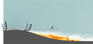
Smooth body separation refers to the flow condition where neither the separation nor reattachment points of a separation bubble are geometrically imposed. As a result, the flow development history (i.e. the influence of pressure gradients and/or compressibility) affects the tendency of the flow to separate. Reference Uzun and MalikUzun & Malik (2022) recently performed a quasi-DNS of flow over a spanwise-periodic Gaussian bump in which the flow separates on the leeward side of the bump due to the mild, adverse pressure gradient. Similarly, the wall-resolved LES of Reference Uzun and MalikUzun & Malik (2019) is an example of shock-induced separation in a transonic flow over a bump. Figure 4 shows a schematic of the bump geometries and the case set-up for both flows. For both flows, an incoming zero-pressure gradient turbulent boundary layer experiences a favourable pressure gradient, which accelerates the flow before eventually experiencing an adverse pressure gradient that leads to flow separation. Although not shown, the variation in the Clauser parameter, Reynolds numbers along the streamwise direction until the point of separation ($x/L \sim 0.1$ for the SBSE and $x/c \sim 0.65$ for the BJ) are significantly different.

Figure 4.

A schematic of the surface geometry over which the turbulent flow separates in the (a) subsonic Boeing speed bump case of Reference Uzun and MalikUzun & Malik (2022) and (b) transonic flow case of Reference Uzun and MalikUzun & Malik (2019). Here $L$ and $c$ are the characteristic lengths for the two cases, respectively; $U_{e}$ is the free stream flow velocity, and the arrows next to it point along the positive streamwise direction.

As seen in figure 5, the proposed model predicts the momentum thickness for both these flows reasonably up to the point of separation (for the transonic flow, Reference Uzun and MalikUzun & Malik (2019) performed their simulations at $Ma = 0.875$ at which the location of the shock, and the separation nearly coincide (Reference Bachalo and JohnsonBachalo & Johnson 1986)). The $Re_\theta$ (right-hand abscissa in figure 5a,b) for both these flows does not monotonically increase as the flow experiences a favourable pressure gradient (not seen in ‘training’ cases). Further, the $Re_\theta$ on the transonic bump reaches values $Re_\theta \sim O(10^4)$, larger than those in the training sets. We remark that inside the separation bubble, the thin boundary layer approximation utilized breaks down, and as such, this model is not expected to perform well.

Figure 5.

Fit of $\theta$ versus the streamwise distance $x$ non-dimensionalized by the respective bump widths. Panel (a) presents the model fit and the true $Re_\theta$ for the Boeing speed bump in Reference Uzun and MalikUzun & Malik (2022), and (b) presents the model fit and the true $Re_\theta$ for the wall-resolved LES (WRLES) of the transonic Bachalo–Johnson bump in Reference Uzun and MalikUzun & Malik (2019). The solid vertical lines denote the separation point as obtained from the reference data. Note that $x/L = 0$ is the position of the apex of the Boeing speed bump, whereas $x/c = 0.5$ is the position of the apex of the transonic bump.

It is also highlighted that the proposed model was derived for incompressible flows and neglected any variations in density in the flow across the boundary layer. The transonic flow in Reference Uzun and MalikUzun & Malik (2019) was locally supersonic in the favourable pressure gradient region exhibiting a density gradient across the boundary layer; the ratio of the mean density in the free stream and the wall $\approx$2, and a normalized density gradient, $\boldsymbol {\nabla } \rho \gg 1$ (the reader is referred to figure 1 in Reference Uzun and MalikUzun & Malik (2019) for more details). A more complete analysis of compressible turbulent boundary layers suggests that the ratio of the free stream to wall temperature (or equivalently densities) should appear as an additional factor in the Taylor series expansion, which may account for some of the observed differences between the reference data and the proposed model. A comparison between the proposed model and the existing methods (in § 3) for flow over the Boeing speed bump geometry is presented in Appendix B.

The proposed model can be used to help predict the conditions under which the separation of the boundary layer is imminent. To date, there have been numerous attempts to characterize this point of separation empirically. Reference AlberAlber (1971) proposed that separation is imminent when $({\theta }/{\rho _e U^2_e}) ({{\rm d} P_e}/{{\rm d} s}) > 0.004$. The exact value of the threshold was determined empirically for some weakly compressible flows and is relatively robust in the presence of weak shocks (Reference Alber, Bacon, Masson and CollinsAlber et al. 1973; Reference AdairAdair 1987). As seen in figure 6 the value of $({\theta }/{\rho _e U^2_e}) ({{\rm d} P_e}/{{\rm d} s})$ is approximately $0.004$ at the location of separation for both the flow over the Boeing speed bump and the flow in the Bachalo–Johnson experiments. For laminar flows, Thwaites also proposed a fit between the shape factor, $H$, and the Holstein–Bohlen parameter, $m$, that allowed computation of the skin friction using the local value of $m$. Using this analysis, the separation boundary for a laminar flow was suggested to be $m=0.09$. Although not shown, we have observed that the two flows considered in this work exhibited separation for different values of $m$, and thus $m$ alone cannot be used to predict flow separation in turbulent flows.

Figure 6.

The variation in the non-dimensional group $({\theta }/{\rho _e U^2_e}) ({{\rm d}P}/{{\rm d}s})$ along the streamwise direction for the (a) Boeing speed bump in Reference Uzun and MalikUzun & Malik (2022) and the (b) transonic Bachalo–Johnson bump in Reference Uzun and MalikUzun & Malik (2019). The dashed vertical lines denote the separation point as obtained from the reference data. Note that $x/L = 0$ is the position of the apex of the Boeing speed bump, whereas $x/c = 0.5$ is the position of the apex of the transonic bump.

Alternatively, it is possible to estimate the value of the Alber separation parameter by using the proposed model. For a locally constant and finite pressure gradient, the proposed model suggests that ${{\rm d}\theta }/{{\rm d}s}$ is a linear function of $({\theta }/{\rho _e U^2_e}) ({{\rm d} P_e}/{{\rm d} s})$ (the reader is referred to (4.3) and the fact that $m/Re_\theta = ({\theta }/{\rho _e U^2_e}) ({{\rm d} P_e}/{{\rm d} s})$). Using the von Kármán integral equation, this equation can be further simplified as

(6.1)\begin{equation} \frac{C_f}{2} \approx \frac{C_c}{2} \frac{\nu}{U_e \theta} + \frac{C_{Re, \infty}}{2} + \left (\frac{C_m}{2} - (2 + H) \right) \frac{\theta }{\rho U^2_e} \frac{{\rm d} P_e}{{\rm d} s}. \end{equation}

In the limit of an asymptotically large Reynolds number ($Re_{\theta } \rightarrow \infty$) flow nearing separation, and estimating $H \approx 2.0$, yields that the separation is imminent when

(6.2) \begin{equation} \frac{\theta }{\rho U^2_e} \frac{{\rm d} P_e}{{\rm d} s} \approx {\frac{- C_{Re, \infty}}{2 \left(\dfrac{C_m}{2} - (2 + H) \right) }} \approx 0.003, \end{equation}

which is similar to the empirical threshold proposed by Reference AlberAlber (1971). It is noted that although $Re_\theta$ does not strictly tend to an infinite value at the point of separation in most flows: for $Re_\theta \gg 600$ at the separation point, the first term on the right-hand side of (6.1) becomes much smaller than the second term ($C_{Re,\infty }/2$), thus removing any explicit dependence of the value of Alber's parameter on $Re_\theta$. It is highlighted that the estimate of $H \approx 2$ is only made to compare the orders of magnitude of the threshold value of $\theta /(\rho _e U^2_e)\, {\rm d}P_e/{\rm d}s$ for flow separation between the proposed model and that of Reference AlberAlber (1971). For instance, if a value of $H = 2.5$ is used, the threshold value (based on the present values of $C_m, C_{Re,\infty }$) of $\theta /(\rho _e U^2_e) \,{\rm d}P_e/{\rm d}s$ for flow separation $\approx$0.0014. Using this threshold value, the error (relative to the true value) in the predicted point of separation is $\Delta x/L \approx 0.06$ (on the Boeing speed bump) and $\Delta x/c \approx 0.04$ (on the Bachalo–Johnson bump), respectively. Similarly, the error incurred upon using a threshold value of $0.003$ (in (6.2)) is $\Delta x/L \approx 0.03$ and $\Delta x/c \approx 0.03$ for the two bump flows, respectively. In this respect, the values of $H \approx 2$ or $H \approx 2.5$ are deemed to lead to the same order of error in determining the separation point.

Equation (6.1) also describes a nonlinear separation and reattachment criterion (in a space spanned by $1/Re_{\theta }$, $H$ and $({\delta ^{*}}/{U^2_e}) ({{\rm d} P_e}/{\rho \,{\rm d} s})$) for turbulent flows over smooth surfaces for a range of Reynolds numbers as

(6.3)\begin{equation} \frac{C_c}{2} \frac{\nu}{U_e \theta} + \left(\frac{C_m}{2} - (2 + H) \right) \frac{\theta }{\rho U^2_e} \frac{{\rm d} P_e}{{\rm d} s} = {-} \frac{C_{Re, \infty}}{2}. \end{equation}

7. Sensitivity analysis of separation using Alber's parameter

Accurate prediction of flows exhibiting separation from mild, adverse pressure gradients remains a pacing item for the development of closure models for both Reynolds-averaged Navier–Stokes and LES. In this section, we explore using the proposed model to quantify the impact of history effects in such flows. The following assumes that the point of separation is determined by Alber's parameter, as was motivated in the preceding section.

In wall-modelled LES, it is difficult to isolate the regions of deficiency of the near-wall model (for predicting the wall shear stress) in non-equilibrium flows, especially in flows undergoing smooth body separation. This is in part because it remains difficult to quantify the importance of history effects in the wall closure approximation. If we denote $J(\theta )_{sep} = -({\theta _{sep}}/{U_{e,sep}}) ({{\rm d}U_{e,{sep}}}/{{\rm d}s})$ as the value of the Alber parameter at the point of separation, then the parameter $({m}/{J_{{sep}}}) ({{\rm d}J_{{sep}}}/{{\rm d}m})$ is a relative measure of the sensitivity of flow separation parameter to upstream modelling deficiencies (quantified via $m$) since the perturbations in $m$ ($\Delta m$ or ${\rm d}m$ in the limit of $\Delta m \rightarrow 0$) can be thought of as arising due to the errors in the prediction of the wall stress. This sensitivity parameter can be re-expressed as

(7.1)\begin{equation} \frac{m}{J_{{sep}}} \frac{{\rm d} J_{sep}}{{\rm d}m} = \frac{m}{J_{sep}} \frac{{\rm d}J_{sep}}{{\rm d}J ( \theta ) } * \frac{{\rm d}J ( \theta ) }{{\rm d}m} = \frac{m}{J_{sep}} \frac{{\rm d}J_{sep}}{{\rm d}J ( \theta) } * \frac{1}{2 Re_{\theta}} = \frac{1}{2} \frac{\theta}{\theta_{sep}} \frac{{\rm d} \theta_{sep}}{{\rm d} \theta} = \frac{1}{2} \frac{\theta}{\theta_{sep}} \frac{1} {\dfrac{{\rm d} \theta }{{\rm d} \theta_{sep}}}. \end{equation}

Equation (7.1) quantifies the expected response in the value of $J_{sep}$ for a given perturbation in $m$. Further, based on the last equality in (7.1), this sensitivity parameter can be completely determined by numerically perturbing the momentum thickness at the true point of separation ($\theta _{sep}$) and integrating (4.3) backward (upstream). This provides the change in $\theta$ at all upstream locations due to a known perturbation in $\theta$ at the true separation point.

Figure 7 suggests that two different mechanisms are important for the two separating flows considered in this article. From figure 7(a), it is clear that for the Boeing speed bump, the sensitivity of Alber's parameter to a perturbation in $m$ is non-local, or that a perturbation in $m$ even far upstream, $30\unicode{x2013}40 \, \delta _{sep}$, will lead to a non-negligible change in $J_{sep}$. However, perturbations in the region after the apex (beyond the vertical dashed line, in the adverse pressure gradient region) are most important in that the imminently separating flow responds to those the most. The curve is increasing in the zero pressure gradient and the favourable pressure gradient region, which implies that the closer the perturbations are made to the separation point, the more responsive the tendency of the flow to separate. These results agree with Reference Devenport and LoweDevenport & Lowe (2022) who suggest that the ‘history effects’ of pressure gradients in a turbulent boundary layer may extend up to 50$\delta$ (where $\delta$ is the local boundary layer thickness). However, in figure 7(b), for the transonic bump, the sensitivity is primarily localized in a smaller region after the apex (less than $5 \delta _{sep}$), localized to the vicinity of the shock (marked by the dashed line). This suggests that for the Bachalo–Johnson bump flow, the prediction of separation is primarily governed by the shock and the adverse pressure gradient in its vicinity, or the upstream history or modelling errors are not that significant. These contrasting mechanisms in the two separating flows considered in this article provide evidence that flow separation can occur due to different flow development patterns.

Figure 7.

The streamwise variation (non-dimensionalized by the boundary layer thickness at the point of separation) of the relative sensitivity of $J_{sep} = -({\theta }/{U_e}) ({{\rm d}U_e}/{{\rm d}s})$ evaluated at the point of separation to the upstream perturbations in the Holstein–Bohlen parameter, $m$, for (a) the Boeing speed bump and (b) the transonic Bachalo–Johnson bump. The dashed lines in panels (a) and (b) correspond to the location of the bump apex and the shock, respectively. Here, $\delta _{sep}$ is the thickness of the boundary layer at the true point of separation.

8. Model limitations

Thus far, the proposed model has been shown to predict momentum thickness in several non-equilibrium turbulent boundary layers reasonably. However, we also highlight some potential limitations of the proposed model in specific flow regimes.

1. (i) Laminar or relaminarizing boundary layers. For laminar boundary layers, the original method of Reference ThwaitesThwaites (1949) is expected to produce more favourable results than the proposed method. This can be seen in that the proposed model's coefficients are larger than the equivalent coefficients in the original Thwaites' method. Further, for highly accelerated boundary layers with significant relaminarization (Reference SreenivasanSreenivasan 1982), the proposed model is not expected to capture the reduced growth of the momentum thickness as the ‘training dataset’ only contains the purely turbulent flow regimes. For instance, although not shown, it was observed that for the strongly accelerated, relaminarizing boundary layer studied in Reference Bourassa and ThomasBourassa & Thomas (2009), the proposed model underpredicts the momentum thickness by approximately 60 % in the regions where the acceleration parameter, $K = \nu /U^2_e \,{\rm d}U_e/{{\rm d} x} \geq 2 \times 10^6$ (region of at least partial relaminarization).

2. (ii) Low Reynolds number turbulent boundary layers. As discussed in the model description, for $Re_\theta \leq 100$, the truncation error in the proposed model may become comparable to the model predictions. Thus, the model can be expected to fail for such low Reynolds numbers.

3. (iii) Large pressure gradients, and separated boundary layers. As also highlighted in § 4, for flows with very large pressure gradients, such that $m/Re_\theta \geq O(10^{-1})$, the proposed linear truncation (4.3) is not expected to determine the growth of the momentum thickness reasonably. Further, beyond the onset of a boundary layer separation, the proposed model has been shown to predict the momentum thickness incorrectly (see § 6.3). Such a flow regime is marked by a strong increase in the shape factor, with $H$, often reaching values higher than $H \gtrsim 2$. These regimes also coincide with sharp rises in the Clauser parameter ($\beta \gg 1$, such as in figure 3) as the shear stress drops to zero near a separation point.

4. (iv) High free stream turbulence. High free stream turbulence values can reduce the wake region of the boundary layer relative to a negligible free stream turbulence case (Reference Thole and BogardThole & Bogard 1996), and increase the skin-friction (Reference Hancock and BradshawHancock & Bradshaw 1983), thus also equivalently increasing ${\rm d} \theta /{{\rm d} x}$. Thus, in the presence of significant free stream turbulence, the present model may underpredict the growth of the momentum thickness. Future research may include the effects of free stream turbulence through an additional eddy-viscosity term such as in Reference VolinoVolino (1998).

5. (v) Wall roughness. In boundary layers with wall roughness, there is an additional drag due to the pressure forces, which shift the mean velocity profile downward relative to a smooth wall (in viscous units). Generally, this form drag is represented in the doubly averaged form of the Navier–Stokes equations as a sink term (Reference Talluru, Djenidi, Kamruzzaman and AntoniaTalluru et al. 2016), which also modifies the von Kármán integral equation relative to (1.2). However, the present model ignores this added drag term and is thus expected to underpredict the growth of momentum thickness.

6. (vi) Compressible boundary layers. As observed on the fore side of the transonic Bachalo–Johnson bump, for a locally supersonic flow, the proposed model overpredicts the momentum thickness as the effect of the Mach number in the von Kármán integral equation has been ignored.

7. (vii) Large Reynolds number limit. For $Re_\theta \rightarrow \infty$, in the absence of any pressure gradient, ${\rm d} \theta /{\rm d}s = C_f/2$ is smaller than the predicted ${\rm d} \theta /{\rm d}s = C_{Re,\infty } /2$ as $C_f$ decreases with $Re_\theta$ (albeit weakly, see Reference Nagib, Christophorou and MonkewitzNagib et al. (2006)). The fitted coefficient, $C_{Re/\infty }$ was based on a boundary layer at an $Re_\theta \sim O(10^4 )$, and hence for a higher Reynolds number, for example, $Re_\theta \geq O(10^5)$ flow, the currently fitted model coefficients may be expected to overpredict the boundary layer growth.

8. (viii) Wall curvature. The effect of surface curvature on the accuracy of the proposed model has been briefly tested using the two bump flows (e.g. on the Boeing speed bump, $\delta /r_w \lessapprox 0.06$). For large curvatures, however, when $\delta /r_w \uparrow$ ($r_w$ is the local radius of curvature of the wall) becomes larger, additional curvature correction terms would need to be included in the proposed model.

Future work may include further improvements to the proposed model to alleviate these model limitations.

9. Concluding remarks

This work presents an extension of the method of Thwaites for determining the momentum thickness for a turbulent boundary layer under the action of pressure gradients. In the limit of large Reynolds numbers, a linear model is hypothesized, such that the Reynolds number and pressure gradient dependence on the growth rate of the momentum thickness can be superposed. A fit for the model coefficients is found using recent high-fidelity simulation data for various boundary layers ranging from Reynolds number, $Re_{\tau } \approx [100, 4000]$ and Clauser parameter, $\beta, \approx [-6, 10]$. Generally, the model predicts the growth of the momentum thickness well for both favourable and adverse pressure gradient flows. The model is also used to derive a condition for imminent separation at high Reynolds numbers, which resulted in similar threshold values as previously work of Reference AlberAlber (1971). An application of the proposed method is demonstrated by estimating the importance of history effects on separation. Specifically, the importance of upstream history effects for the Boeing speed-bump flow is quantified. For a transonic bump flow, it is shown that only local perturbations just upstream of the shock location cause significant changes to the separation location.