


1. Introduction
The Filchner-Ronne drainage basin of Antarctica (3.7 million km2 including the ice shelves; Zwally and others, Reference Zwally, Giovinetto, Beckley and Saba2012) contains 25% of all ice in the Antarctic ice sheet (Morlighem and others, Reference Morlighem2020), and supports the second largest ice shelf on the continent (430 000 km2). There is uncertainty about the sign of ice mass change across this region at present (Rignot and others, Reference Rignot2019), and over the 21st century the ice mass balance of this region is not expected to change drastically (Golledge and others, Reference Golledge2019). However, given the scale of this region it remains important to understand how changing surface and ocean conditions impact the ice shelf and ice sheet. Until the end of the 21st century, changes in snow accumulation are considered to be the largest contributor to the mass balance change in this region (Hill and others, Reference Hill, Rosier, Gudmundsson and Collins2021).
The Filchner-Ronne Ice Shelf is important to the stability of ice mass in the region due to buttressing effects (Fürst and others, Reference Fürst2016), and thinning of the ice shelf can increase ice loss across the region (Reese and others, Reference Reese, Gudmundsson, Levermann and Winkelmann2018a). Therefore projecting the future of the ice shelf is important for projecting the future sea level contribution of this region. Of the threats to the ice shelf, surface melt does not provide much risk. Among all Antarctica ice shelves, the Filchner-Ronne Ice Shelf has some of the lowest surface melt rates (Jakobs and others, Reference Jakobs2020) and fewest days of surface melt (Johnson and others, Reference Johnson, Hock and Fahnestock2021), and is well below the assumed-threshold to risk collapse due to surface melt driven hydrofacture (Trusel and others, Reference Trusel2015). Ocean-driven changes in subshelf melt, however, can provide much higher melt rates across the region under projected emission scenarios (Naughten and others, Reference Naughten2021).
Ocean surface temperatures and circulations interact with the ice shelf through multiple processes. Increased surface temperatures reduce sea ice formation, which could initially decrease basal melting on the Filchner-Ronne Ice Shelf as there will be less high-salinity, dense seawater to drive circulation into the freshwater cavities under the Ronne Ice Shelf (Nicholls and Østerhus, Reference Nicholls and Østerhus2004). The converse has been directly observed, as increased sea ice production in the Weddell Sea since 2015 has strengthened this circulation (Hattermann and others, Reference Hattermann2021). Greater temperature increases resulting in further thinning of Weddell Sea sea ice, however, could potentially lead to warm deep water from the Weddell Sea entering the subshelf environment, which could greatly increase subshelf melting (Hellmer and others, Reference Hellmer, Kauker, Timmermann, Determann and Rae2012), and evidence suggests this process has already begun (Darelius and others, Reference Darelius, Fer and Nicholls2016). These phenomena have been reproduced with coupled ocean and ice sheet models by Naughten and others (Reference Naughten2021), who found that a global mean surface temperature increase of 7 °C relative to 1850 is required to destabilize the ice shelves in this region, although moderate warming has an impact on mass fluxes and sea level contributions.
The aim of this work is to simulate the response of ice in the Filchner-Ronne region to several climate change and ocean warming scenarios and to characterize the probability density function of contribution to sea-level at 2100 for each scenario. The 21st century projections presented in this study under RCP scenarios complement Hill and others (Reference Hill, Rosier, Gudmundsson and Collins2021), who used the finite-element ice sheet model Úa to study the same region and time period. Here we elaborate on their work by taking an ensemble approach using the computational efficiency of the Parallel Ice Sheet Model (PISM; Bueler and Brown, Reference Bueler and Brown2009) to provide numerical simulations at high resolution. Uncertainties related to ice dynamics translate to uncertainties in sea-level projections (Zeitz and others, Reference Zeitz, Levermann and Winkelmann2020), and a number of parameters in our our ensembles are calibrated to reproduce contemporary surface speeds using a Bayesian method of surrogate model analysis. This study also provides a unique quantification of the sensitivity of land ice in this region to increased ocean temperatures.
2. Methods
2.1. Overview
We applied ensembles of PISM simulations to study the twenty-first century evolution of ice in the Filchner-Ronne region. The workflow is illustrated in Fig. 1. We started with a spun-up, thermodynamically evolved model of the Filchner-Ronne region of Antarctica. We then calibrated a number of parameters controlling ice flow with a Bayesian optimization approach using a comparison to real world observed ice speeds. We applied this model to several scenarios, including using surface and ocean forcing from RCP 2.6 and 8.5, and also to a set of scenarios involving an immediate step change in ocean temperature with constant climate forcing in order to test the response of this region to increased ocean warming.
Description of modeling workflow. Names of topics in the workflow refer to section names.

2.2. Model description
PISM uses a hybrid stress balance that solves numerical approximations to the shallow ice and shallow shelf equations (Bueler and Brown, Reference Bueler and Brown2009). The effective viscosity of glacier ice, η, is given by:

where $\tau _{\textrm e}$ is the effective stress, E is the enhancement factor, A is the enthalpy-dependent rate factor, and n is the exponent of the power law. The small constant $\epsilon$
 (units of stress) regularizes the flow law at low effective stress, avoiding the problem of infinite viscosity at zero deviatoric stress. The pseudo-plastic power law (Schoof, Reference Schoof2010) relates bed-parallel shear stress, τb, and the sliding velocity, ub:
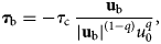
where τ c is the yield stress, q is the pseudo-plasticity exponent, and u 0 = 100 m yr−1 is a threshold speed. We assume that yield stress τ c is proportional to effective pressure N (‘Mohr-Coulomb criterion’: Cuffey and Paterson, Reference Cuffey and Paterson2010),

where ϕ is the till friction angle given as a function of bed elevation z:

The parameter b range (m) is defined as b range = b max − b min and is used as a tuneable parameter in this study. The effective pressure N is given by Tulaczyk and others (Reference Tulaczyk, Kamb and Engelhardt2000) and Bueler and van Pelt (Reference Bueler and van Pelt2015):

Here δ is a lower limit of the effective pressure, expressed as a fraction of overburden pressure, e 0 is the void ratio at a reference effective pressure N 0, C c is the coefficient of compressibility of the sediment, W is the effective thickness of water in the till, and W max is the maximum amount of basal water. We use a non-conserving hydrology model that connects W to the basal melt rate $\dot B_{{\rm b}}$ (kg m−2 a−1; Tulaczyk and others, Reference Tulaczyk, Kamb and Engelhardt2000):

where ρ w is the density of water and C d = 1 mm yr−1 is a fixed drainage rate.
PISM has been used in many ice sheet model intercomparison projects (e.g. Seroussi and others, Reference Seroussi2019; Cornford and others, Reference Cornford2020; Levermann and others, Reference Levermann2020; Seroussi and others, Reference Seroussi2020; Sun and others, Reference Sun2020), and PISM modeling studies have helped projections of the trajectories of the Greenland and Antarctic ice sheets (e.g. Aschwanden and others, Reference Aschwanden2019; Golledge and others, Reference Golledge2019).
2.3. Model setup and initialization
The Filchner-Ronne drainage basin is represented in PISM using a 1799 km × 2159 km domain (Fig. 2). The maximum extent of the ice shelf is constrained to the extent in 2016 to prevent further ice shelf advance, although ice shelf calving fronts are allowed to retreat. At the domain boundaries, we forced the gradients of ice thickness and surface elevation to be zero, and set ice thicknesses to zero beyond the boundary. Inside that region ice is free to evolve.
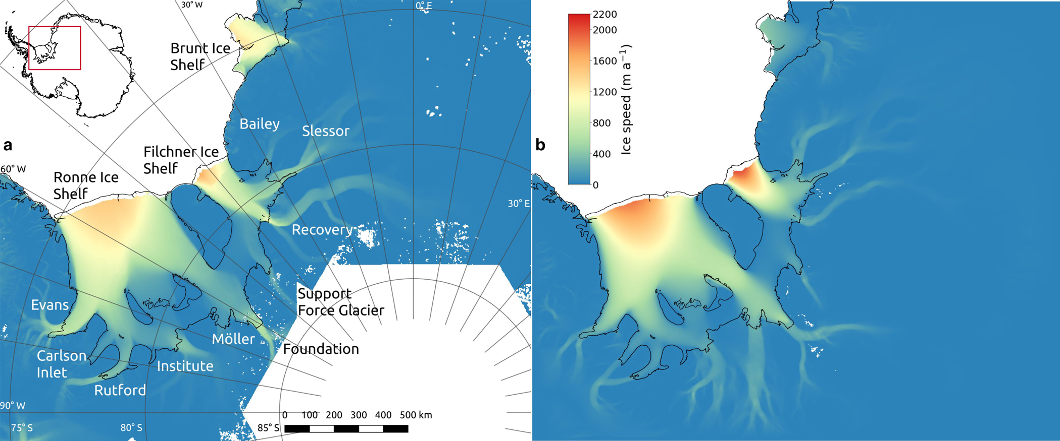
Map of modeled domain showing observed and modeled ice velocities. (a) Observed 2018 ice velocities from ITS_LIVE, with ice streams and ice shelves labeled. (b) Modeled ice velocities, showing median 2018 velocity for each gridcell. Grounding lines and ice shelf bounds are shown in black, from the 2020 outlines from SCAR, which are close to the grounding line locations of at the start of the model run.
As ice is a good insulator and the thermal regime needs multiple millennia to be in equilibrium with the climate conditions at the surface, we perform a step-wise initialization method. The ice sheet requires time to reach thermal equilibrium as well as dynamic equilibrium, as dynamics are a function of temperature. A simulation of temperature evolution at 10 km grid resolution keeping the geometry fixed was run for approximately 100 000 years, followed by a 10 000 year model run to reach dynamic equilibrium, and then 1000 years at 1 km grid resolution with fixed ice thicknesses. Finally, we updated bed topography and present day thicknesses from Bedmap2 (Fretwell and others, Reference Fretwell2013) to BedMachine (Version 2; Morlighem and others, Reference Morlighem2020) and performed a 500 year simulation to reach a new thermal equilibrium. The switch from Bedmap2 to BedMachine was done in order to utilize existing work at recreating modern the dynamic and thermodynamic conditions of Antarctica within PISM. Directly following the switch from Bedmap2 to BedMachine, ice was frozen to the bed along some ice streams due to energy conservation as some ice thickness increased, and the additional time was required to restart the ice stream activity.
2.4. Model forcing
PISM was forced by the 1950–2014 mean near-surface air temperature and climatic mass-balance fields from the regional climate model RACMO2.3p2 remapped to 1 km resolution (van Wessem and others, Reference van Wessem2018). RACMO was forced with the Community Earth System Model Version 2 (CESM2; Danabasoglu and others, Reference Danabasoglu2020). During the model setup and initialization, ocean temperature and ice shelf basal mass fluxes were generated with the Finite Element/columE Sea ice-Ocean Model (FESOM; Wang and others, Reference Wang2014), and applied using constant melt rates. In the Filchner-Ronne region FESOM is capable of reproducing the subshelf circulation to produce realistic shelf basal melt fields (Timmermann and Goeller, Reference Timmermann and Goeller2017).
For model calibration and future projections, we calculated ice shelf basal mass flux using PICO (Reese and others, Reference Reese, Albrecht, Mengel, Asay-Davis and Winkelmann2018b). PICO is an ocean module parametrization which assumes warm water reaches the grounding line of the ice shelf and then basal melt is modeled using the overturning as that water rises and cools with melt and sub-ice shelf geometry. The inputs for PICO include the mean ocean salinity and potential temperature at the depth of the continental shelf off the ice shelf front across the entire drainage basin and a few other parameters, most importantly an ocean overturning coefficient $\gamma _T^\ast$ and heat exchange coefficient C. Although PICO does not capture the complexities of ocean circulation underneath the ice shelf of a more advanced ocean model (e.g. FESOM), it reproduces typical melt patterns within the range of observed melt rates around Antarctica (Reese and others, Reference Reese, Albrecht, Mengel, Asay-Davis and Winkelmann2018b) and provides a realistic method to model melt using different ocean temperatures (Hill and others, Reference Hill, Rosier, Gudmundsson and Collins2021).
Calving is controlled by an eigen-calving scheme which has been found to be appropriate for Antarctic ice shelves (Levermann and others, Reference Levermann2012). Calving is proportional to the product of eigenvalues of strain rates for diverging flow, with a coefficient K. Overall ice mass has not been found to be sensitive to reasonable values of the parameter K. Albrecht and others (Reference Albrecht, Winkelmann and Levermann2020a) tested values of K between 1016 and 1018 m s and found this law caused present-day calving to occur largely in areas that provide little buttressing; calving occurred within the ‘passive ice shelf’ areas described by Fürst and others (Reference Fürst2016). As such we set the value of K here to be 2 × 10¹⁵ m s based on a manual calibration, but we do not tune it further. An additional minimum ice shelf thickness criteria of 100 m is applied, with thinner ice calved off.
2.5. Model calibration
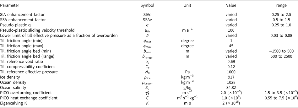
Uncertainties in ice flow parameters can have a large impact on projections of ice mass changes in modeling studies (Albrecht and others, Reference Albrecht, Winkelmann and Levermann2020a; Zeitz and others, Reference Zeitz, Levermann and Winkelmann2020). To mitigate this issue, we calibrated six parameters controlling ice flow to better reproduce observed surface speeds These parameters are: the Shallow Ice and Shallow Shelf enhancement factors (SIAe and SSAe, respectively), exponent of the pseudo-plastic sliding law (q), lower limit of till effective pressure as a fraction of overburden (δ), till friction angle depth minimum (b min) and till friction angle depth range (b range). Naming conventions follow PISM documentation (The PISM Authors, 2018), except for δ which is called till effective fraction overburden in PISM, and b range. The applications of these parameters are described by equations 1–5. The values of model parameters which were not varied come from PISM default values, Albrecht and others (Reference Albrecht, Winkelmann and Levermann2020a), or manual calibration.
The enhancement factors SIAe and SSAe are coefficients applied to the Glen-Paterson-Budd-Lliboutry-Duval flow law (Lliboutry and Duval, Reference Lliboutry and Duval1985), with enhancement factors for shelf/stream plug flow usually being expected to be below 1 (Ma and others, Reference Ma2010). Sliding is controlled by a power law relating velocities and basal shear stress (Eqn. (2)), with exponent q such that q = 0 is coulomb-plastic sliding and q = 1 is purely linear sliding. Sliding occurs when the driving stress is greater than a basal shear stress, which is a function of a number of parameters including the till friction angle. The till friction angle varies linearly with bed depth from a minimum angle ϕ min at b min to a maximum angle ϕ max at b max (Eqn. (4)). The ranges of parameter values used in this calibration are shown in Table 1. To determine the range of values for the calibrated parameters, the entire calibration process was done twice, the first time with a wider range of values, and the second time with a more narrow range. The parameter values for each ensemble were drawn using Sobol Sequences, which is a quasi-random sampling method intended to evenly search the parameter space.
Model parameters used in PISM. Parameters that were tuned during the calibration process have the values listed as ‘varied’ range of values tested listed. The varied PICO parameters were not tuned in the calibration
Our calibration closely follows the methodology of Brinkerhoff and others (Reference Brinkerhoff, Aschwanden and Fahnestock2021) which estimated the joint parameter distributions given observations using Markov-chain Monte Carlo sampling (MCMC). We rendered the problem tractable by constructing an artificial neural network to act as a surrogate for the ice flow model, which provided a mapping from ice flow parameters to surface speeds.
To begin we created a training dataset with a 300 member model ensemble. For each ensemble member we then ran PISM forward for 50 years at 2 km resolution while keeping atmosphere and ocean forcing constant. Ocean forcing was provided by PICO using modern temperatures and salinities (Schmidtko and others, Reference Schmidtko, Heywood, Thompson and Aoki2014), and using the PICO default parameters for ocean overturning and heat exchange coefficients in PISM (2 × 10⁻⁵ m s−1 and 1 × 10⁶ m6 s−1 kg−1, respectively). The values of the constant model parameters are given in Table 1. For each of the six calibrated parameters listed above, we drew values using Sobol Sequences from within their respective ranges.
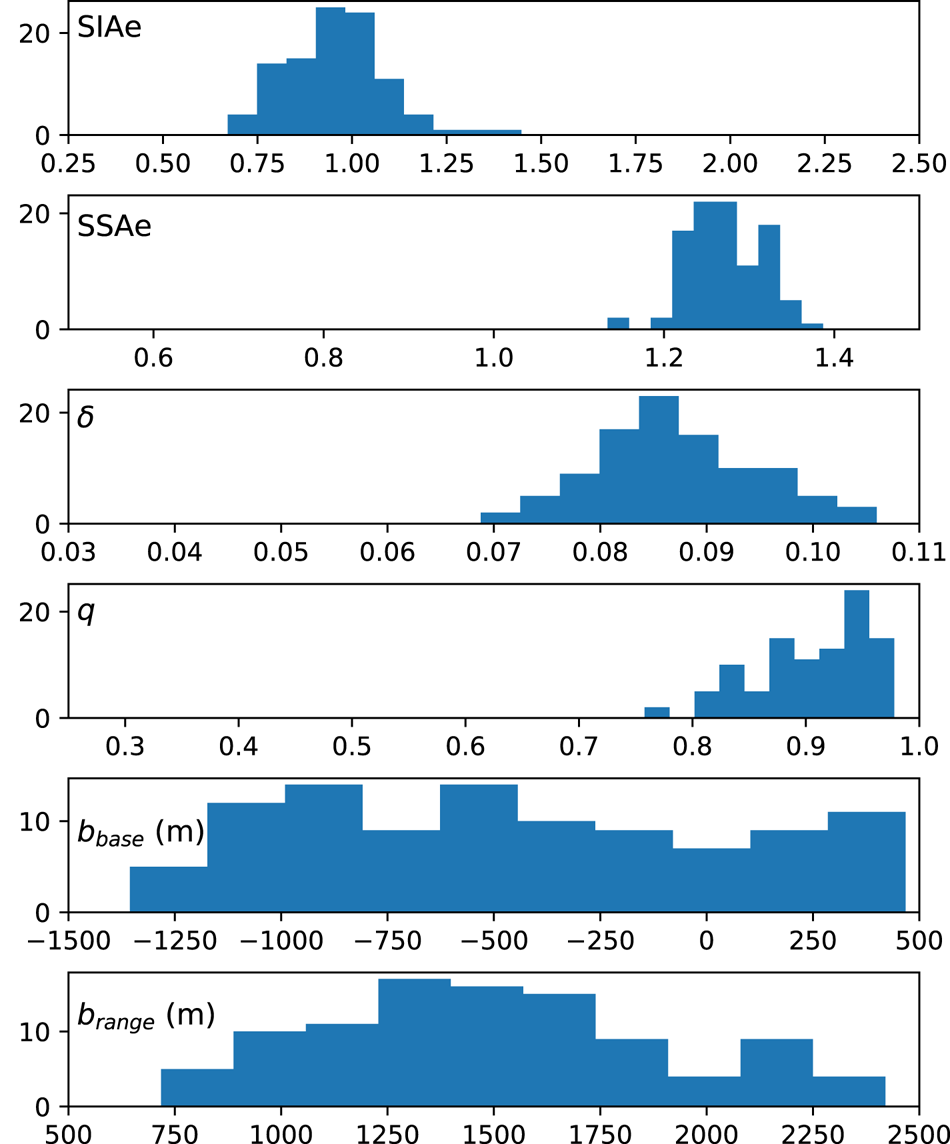
We extracted the ice surface speeds from the training model runs and used principal component analysis to produce a set of ≈50 basis functions, enough to describe 99.95% of the velocity variability. Then we trained an artificial neural network-based surrogate model to map parameter combinations to the principal components and recover the velocity field by multiplying the principal components and the basis functions. Finally, we estimated the joint posterior parameter distributions by using MCMC to draw 105 samples, which were compared to observed surface speeds taken from the ITS_LIVE map of 2018 velocities (Gardner and others, Reference Gardner, Fahnestock and Scambos2019). The MCMC sampling was done in log-space for ice speeds. The observed ice velocities were regridded to the 2 km model grid using bilinear interpolation. Velocities from 2018 were used because they were the most recent available when the comparison was carried out. We used one year of velocity data for this analysis. The annual variation surface speed is very low for locations with speed above 50 m a−1 in the ITS_LIVE record (between 2014–2018 the average standard deviation of surface speed was 0.005 of its magnitude for these locations). Surfaces with slower speeds had higher annual variability, although the interannual variability appears randomly distributed in space so is unlikely to have a strong impact on the parameter calibration which optimizes parameters across the entire domain. From the posterior distributions (shown in the supplementary material) we drew parameter samples for our study scenarios.
We use these parameter sets for each of the climate scenarios in this study, and one of these sets is shown in Fig. 3. A comparison of the observed surface speeds in 2018 and the simulated median speed for each gridcell is given in Fig. 2. The modeled surface velocities are drawn from a scenario with the same climate forcing as the calibration model runs. Overall, speeds are reproduced to within 100 m a−1 near the grounding lines of some of ice streams, including the Bailey, Slessor, and Support Force Glacier (Fig. 2). The most prominent differences between model and observations are higher observed than modeled ice speeds along the ice streams of the southwestern Ronne Ice Shelf, especially including the Evans and Rutford ice streams. Our model has ice draining into the southwestern Ronne Ice Shelf from Carlson Inlet and the Rutford Ice stream, yet presently all ice flows out through the Rutford Ice Stream instead (Fig. 2a). It has been suggested that Carlson Inlet was an active ice stream as recently as several hundred years ago (Vaughan and others, Reference Vaughan, Corr, Smith, Pritchard and Shepherd2008), although other field observations instead suggest Carlson Inlet is not a periodically activating ice stream at all (King, Reference King2011). In our model the Möller Ice Stream has much higher ice velocities and a much greater extent than observations. The goal of the ensemble parameter optimization was to best reproduce ice velocities across the entire region, and as such parameters are not tuned to correctly represent the behavior of individual ice streams.
Frequency of parameter values in the ocean sensitivity analysis ensembles, shown here as the total occurrences for each range. Parameter values were sampled from the parameter posterior distributions, shown in Fig. S1.
2.6. RCP scenarios
In a first set of experiments, we assessed the region's response to the projected range of 21st century climate forcing. We used anomalies of mean annual ocean potential temperature, near-surface air temperature, and climatic mass balance for 2015–2100. For ocean temperatures, we applied a linearly increasing annual ocean potential temperature anomaly in PICO, with the annual rate of increase obtained from the mean value of ocean potential temperature change in the Weddell Sea region over 1995–2100 at 400–600 m depth from Little and Urban (2016) for RCP 2.6 and 8.5. These anomalies were added to the observed 2014 ocean potential temperatures from Schmidtko and others (Reference Schmidtko, Heywood, Thompson and Aoki2014), with salinity held constant.
Several climate parameters varied between ensemble members, and these were drawn in a different manner. Within PICO, the parameters for overturning coefficient $\gamma _T^\ast$ and heat exchange coefficient C have a strong impact on melt (Reese and others, Reference Reese, Levermann, Albrecht, Seroussi and Winkelmann2020). We drew values for these parameters from within the most plausible range found by Reese and others (Reference Reese, Gudmundsson, Levermann and Winkelmann2018a). Specifically, Fig. 4 of Reese and others (Reference Reese, Gudmundsson, Levermann and Winkelmann2018a) identified the 14 most realistic $\gamma _T^\ast$
 and C value combinations, and for each ensemble member we randomly chose one of those combinations and then uniformly drew $\gamma _T^\ast$
 and C values from within the range of values closest to that combination. This resulted an equal chance of values of C to be less and greater than 1 × 10⁶ m6 s−1 kg−1. We drew values in this manner to match our knowledge of the plausible parameter configurations, and not skew our values of C to be too high as to likely overestimate basal melt.
For the near-surface air temperatures and climatic mass balance, we obtained annual anomaly values from three Earth System Models (ESMs) for RCP 2.6 and 8.5. These three models, as prepared by Barthel and others (Reference Barthel2020) at 2 km resolution, are the Norwegian Climate Center's ESM (NorESM1-M), Community Climate System Model (CCSM4), and the atmospheric chemistry-coupled ESM from the Model for Interdisciplinary Research on Climate (MIROC-ESM-CHEM). The temperature and mass balance anomalies were applied to the mean 1950–2015 climatic mass balance and near-surface temperature fields (van Wessem and others, Reference van Wessem2018). We ran 200 simulations at 2 km resolution for both RCP 2.6 and 8.5, and we randomly assigned one of the three surface anomaly models to each ensemble member, with each of the three models being used between 66 and 68 times.
2.7. Ocean warming scenarios
For a second set of experiments, we tested the sensitivity of ice in this region to thinning of the ice shelf in response to step change increases in ocean temperatures. These are not based on direct climate projections but rather help to explore the characteristics of the response of this region to increased ice shelf melt. We produced a set of scenarios involving raising present-day ocean potential temperatures at depth by 1–6 $^\circ$ C at 1 $^\circ$
 C intervals. These potential temperature changes were applied to present day ocean temperatures (Schmidtko and others, Reference Schmidtko, Heywood, Thompson and Aoki2014) as a step change. For surface temperature and climatic mass balance we used the RACMO 1950–2014 mean values. We will refer to these as the +1 $^\circ$
 C to +6 $^\circ$
 C ocean warming scenarios and an additional control scenario was run with constant climate and no ocean warming enforced. For each scenario we ran 100 ensemble members at 2 km resolution from 2015–2100, holding ocean and surface forcing constant, aside from the step change in ocean potential temperature at the beginning. The ocean overturning and heat exchange coefficient parameters in PICO were also held constant.
Only the lowest warming scenario presented here is consistent with projected ocean warming at depth, whereas the ocean temperature scenarios beyond +1 $^\circ$ C are well outside the range of 21st century warming under the higher RCP 8.5 scenario (Little and Urban, Reference Little and Urban2016). However, changes in ocean circulation forced by changes in surface winds, potentially possible in the 21st century, can cause an order of magnitude increase in ice shelf melting in the region (Hazel and Stewart, Reference Hazel and Stewart2020; Naughten and others, Reference Naughten2021). The higher end of these warming scenarios are well outside the range found in century-scale projections, but the +6 °C warming scenario provides a forcing comparable to, and perhaps more realistic than, removing all floating ice instantaneously as in the Antarctic Buttressing Model Intercomparison Project (Sun and others, Reference Sun2020).
3. Results
3.1. Model projections
Ice mass increases across the region between 2015 and 2100 for both the RCP 2.6 and RCP 8.5 scenarios (Fig. 4a). There is a significant overlap between the two scenarios, and the median of ice above flotation remains similar, although the uncertainty becomes much greater for RCP 8.5, with the possibility for greater mass losses and mass gains. The mass gains at 2100 correspond to a global mean sea level reduction of 24±7 mm for RCP 2.6 (a gain of 8900±2500 Gt ice above flotation) and 28±9 mm for RCP 8.5 (a gain of 10 300±3200 Gt ice above flotation), assuming a global ocean area of 362.5 × 10⁶ km2. The possibility for positive contribution to sea level exists in the RCP 8.5 scenarios with the most extreme basal melt. Over the entire region, grounded ice thickened at a mean rate of 0.32 m per decade for both RCP 2.6 and 8.5. The probability density function of sea level contribution at 2100 appears somewhat bimodal for RCP 2.6, and this is a result of using multiple discrete sources for surface temperature and climatic mass balance anomalies. The scenarios using CCSM4 and MIROC-ESM-CHEM have greater rates of increase of climatic mass balance over the region than the NorESM1-M scenario does.
Model ensemble projections of the RCP scenarios over 2015–2100 for cumulative change in ice mass above flotation and grounding line mass flux, showing ensemble mean (solid line) and 90% credible interval (shading), with ensemble probability density at 2100 given.
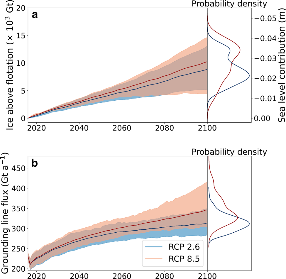
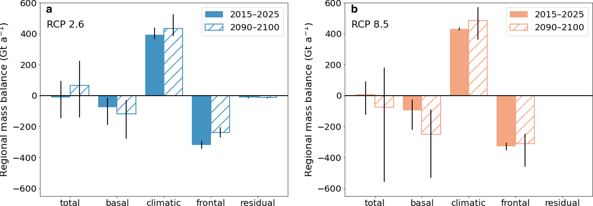
The 21st century mass gains in this region are driven by increased surface accumulation and aided by decreasing frontal ablation, which both compete with increased basal melt (Fig. 5). Across the entire domain, the total annual mass balance increased by 76 Gt a−1 for RCP 2.6 between 2015–2025 and 2090–2100 and decreased by 84 Gt a−1 for RCP 8.5. Both scenarios saw a small increase in surface mass balance due to accumulation, yet RCP 8.5 saw much greater ice shelf basal melt rates due to the warming ocean. Within RCP 8.5, certain combinations of the ocean overturning and heat exchange coefficient parameters of PICO were able to produce very high basal melt rates.. Rates of ice losses due to frontal ablation (the sum of mechanical iceberg calving and ice flowing past the prescribed extent) start out as a large part of the mass budget and decrease over the first couple of decades as the eigencalving mechanism forces the ice shelf into a more stable configuration. Calving begins to trend upward again in the second half of the century under RCP 8.5, whereas it remains constant under RCP 2.6. A full breakdown of mass balance terms over time for each scenario is supplied in the supplementary material (Fig. S2), with a split between frontal ice discharge and calving.
Mass balance components averaged for two decadal periods for (a) RCP 2.6 and (b) RCP 8.5. Fluxes are summed over the entire simulated region, except for the basal balance which only includes the flux over the ice shelves (positive indicates freeze-on). The frontal balance includes ice shelf calving and ice flowing across the prescribed frontal extent limit. The residual balance accounts for any other mass fluxes. Ice shelf area decreased by 8,200 km2 (6.3% of initial area) for the RCP 2.6 scenario and 11 600 km2 (2.6%) for the RCP 8.5 scenario.
The highest increases in ice shelf basal melt occur near the grounding lines, and correspondingly the grounding line mass fluxes increase over the 21st century (Fig. 4b). Simulations using forcing from the RCP 8.5 emission scenario contain more total ice above flotation, but also have higher basal melt rates and an increase in grounding line flux. Grounding line fluxes increase non-linearly with ocean temperature over this time period, similar to the findings by Hill and others (Reference Hill, Rosier, Gudmundsson and Collins2021). We find the rate of ice lost through the grounding lines increases quickly at the beginning and slows down around 2040–2060, which is more pronounced for RCP 2.6 than for RCP 8.5.
3.2. Ocean temperature sensitivity
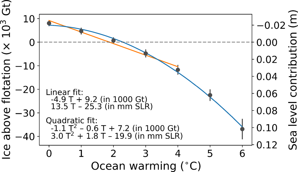
Increased ocean temperatures are directly related to ice mass loss in the scenarios involving step changes to ocean temperatures while holding the surface mass balance forcing constant (Fig. 6). The +1 $^\circ$ C ocean warming scenario resulted in +11 mm contribution to sea level at 2100 compared to the control scenario with constant climate. While Mengel and others (Reference Mengel, Feldmann and Levermann2016) found the relationship of sea level contribution to be linear with climate forcing, our results demonstrate a quadratic relationship with ocean temperature provides a much better fit than a linear one when more extreme forcing scenarios are included (Fig. 6). The rate of mass loss with temperature increased at higher ocean temperatures, and the second derivative of sea level contribution with ocean temperature is +6 mm $^\circ$
 C−2.
C−2.
Ice mass above flotation at year 2100 for seven ocean temperature increase scenarios, with 90% credible interval of mass shown. Orange line shows the linear fit of the mean ice mass above flotation with ocean temperature over the interval of the control scenario to the +4 °C scenario, while blue shows the second-order polynomial fit over the whole domain, for ocean temperature warming T.
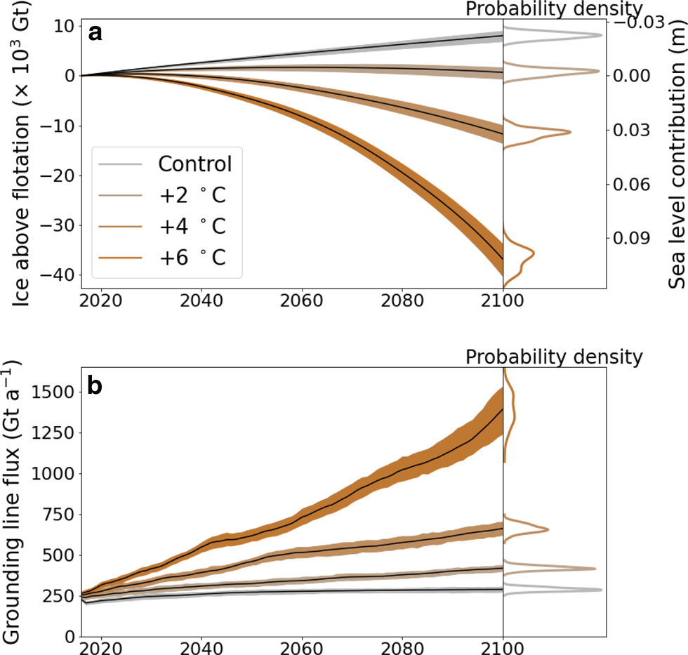
The trajectories of ice mass above flotation diverge rapidly between the different ocean-forcing scenarios (Fig. 7a). Scenarios with the least ocean warming experience gains in ice mass above flotation, up to −22 ± 2 mm sea level contribution. At +2 $^\circ$ C the trend reverses, with ice mass plateauing in the middle of the 21st century and then trending negative, resulting in near-zero total change in sea level contribution at 2100. The +6 $^\circ$
 C scenario shows rapid mass losses, and loses −36 800 ±2200 Gt ice above flotation at 2100, for a sea level contribution of +102±6 mm (Fig. 7a) with greatly increased grounding line fluxes (Fig. 7b). The rate of mass loss with time in this region due to ocean-driven ice shelf retreat has previously been found to be linear (Mengel and others, Reference Mengel, Feldmann and Levermann2016), and we find a near-linear response with time after mid-century for every scenario except the +6 C$^\circ$
 ocean warming step change scenario.
Model ensemble projections of the ocean warming scenarios over 2015–2100 for cumulative change in ice mass above flotation and grounding line mass flux, showing ensemble mean (solid line) and 90% credible interval (shading), with ensemble probability density at 2100 given.
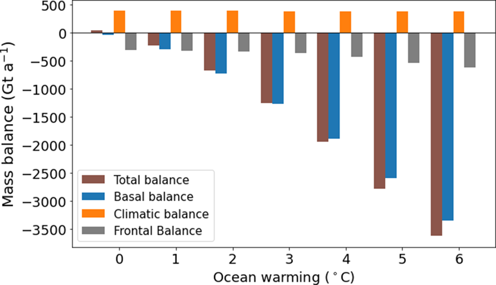
A comparison of the components of the mass budget highlight the severity of forcing provided by ocean temperatures in these scenarios (Fig. 8). The surface climate forcing uses 1950–2014 mean values from RACMO, leading to surface mass gains of 392 Gt a−1 across the entire region over 2015–2100. The ice shelf basal mass balance dominates the total balance with increasing ocean temperature. In the control scenario with constant climate the ice shelf experiences basal melt at a spatially averaged rate of 70 mm a−1 in 2015. However, these melt rates are much higher near the grounding line and lower across the ice shelves, with the front of the Ronne Ice Shelf experiencing basal mass gains due to freeze-on, at approximately a rate of 60 mm a−1. At present, the amount of mass gained due to basal freeze-on has been observed to be approximately 38% of the size of mass lost due to basal melt (Moholdt and others, Reference Moholdt, Padman and Fricker2014), and we find this to be 41% in 2015 in our control scenario. With ocean warming of +1 $^\circ$ C or greater, basal mass gains decrease and are only 10% or less of the absolute magnitude of ice shelf basal mass losses. With increasing ocean temperatures, we find that the mean 2015–2025 basal balance decreases at a rate of −562 Gt a−1 $^\circ {\rm C}^{-1}$
 .
.
Mass balance components averaged over 2015–2025 for each scenario of constant surface forcing and given step changes in ocean temperature. The components of flux are the same as Fig. 5. The 0 $^\circ$ C ocean warming category is the control scenario with constant climate. Ice shelf area decreased by 6600 km2 (1.5% of initial area) for the control scenario.
3.3. Grounding line retreat
An increase in ocean temperature leads to increased sub-shelf melt, resulting in grounding line retreat. The areas around the Filchner-Ronne Ice Shelf where ice currently grounded comes afloat by 2100 or ice currently afloat becomes grounded are shown in Fig. 9. Grounding line retreat is limited in the control simulation, +1 °C warming scenario, and RCPs 2.6 and 8.5 scenarios, largely restricted to retreat on the Slessor Ice Stream for the Filchner Ice Shelf and Institute Ice Stream for the Ronne Ice Shelf. However, with greater warming the retreat becomes more pronounced. Among the control scenario and ocean temperature warming scenarios, the total amount of grounded ice by 2100 decreased with ocean temperature at a linear rate of −23 200 km2 $^\circ$ C−1 (r 2 = .99, p < 0.001), which accounts for 1% of the total initial ice-covered area of the domain.
Areas that become grounded (ΔA g) or ungrounded (ΔA u) by 2100 relative to 2015 for given scenarios. Each map shows probability across all ensemble members for that scenario. The gray shaded areas show the initial 2018 configuration of grounded and floating ice in the model.
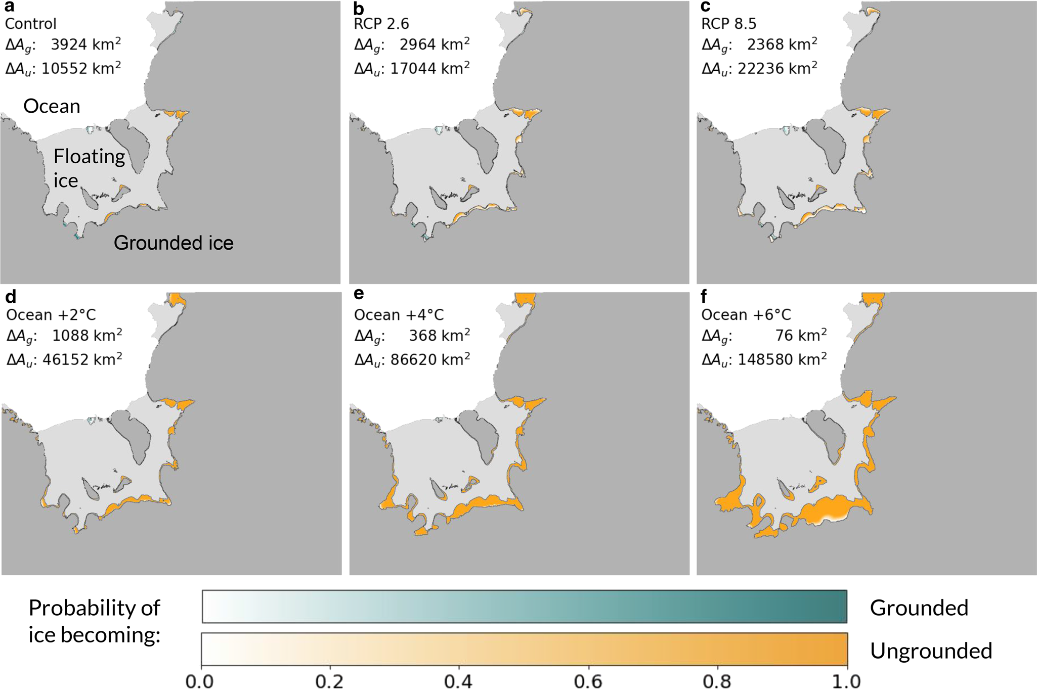
The +2 °C ocean temperature scenario marks the point where the retreat begins to surpass advance. The region experiences mass gain over the first half of the time span (Fig. 7a), with ice shelf basal mass loss rates of 720 Gt a−1 in 2015 in this scenario (with a spatial average of 1.31 m a−1 for floating ice). The mass change of the region only turns negative in the later half of the time span, and because the surface mass balance and ocean temperatures remain constant, this mass loss is a product of dynamical effects of the increased grounding line thinning and retreat. At higher ocean temperatures, we find the greatest retreat to be on the Möller and Institute ice streams, which agrees with previous work suggesting that once retreat is initiated on those ice streams it will not quickly stop, whereas other ice streams could find new equilibria (Wright and others, Reference Wright2014). Our modeled time period runs to 2100, and so potential further grounding line changes due to mass imbalances beyond 2100 are not captured here. In the RCP 8.5 scenario the total mass balance across the region will likely be negative by 2100 (Fig. 5b), yet at 2100 the thinning ice shelf had yet to result in reduced ice above flotation in all but the scenarios with the greatest amount of basal melting (Fig. 4a).
4. Discussion
4.1. Mass trends
The Filchner-Ronne region has not had a significant negative trend ice mass in recent decades (Zwally and others, Reference Zwally, Robbins, Luthcke, Loomis and Rémy2021) even though overall the Antarctic ice sheet has been losing mass (−110 to −148 Gt a−1; Rignot and others, Reference Rignot2019) and is projected to continue to lose mass in the 21st century (Seroussi and others, Reference Seroussi2020) under climate projections from the Coupled Model Intercomparison Project Phase 5 (CMIP5). Cumulatively the ice drainage basins in this study area are in near balance or even have a slight positive trend in mass (−4 to 5 Gt a−1; Rignot and others, Reference Rignot2019), and we project the region to maintain a slight positive trend in ice mass through the 21st century (Fig. 4a).
We find ice thickening will continue at spatially averaged rates of 0.13 m, 0.09 m, 0.04 m decade−1 under constant climate, RCP 2.6, and RCP 8.5, respectively. Near the front of the Filchner-Ronne Ice Shelf, we project thickening of 5–10 m by 2100. Upsteam of the grounding lines, inland patterns of thickness change are driven by the spatial variability in climatic mass balance (Fig. 10). Our results are in good agreement with earlier modeling studies (Golledge and others, Reference Golledge2019; Hill and others, Reference Hill, Rosier, Gudmundsson and Collins2021) which suggest that the Filcher-Ronne area is unlikely to contribute significantly to sea level by the end of the 21st century as increased accumulation upstream of the grounding lines is expected to offset the effect of limited increases in basal melting. Golledge and others (Reference Golledge2019); Hill and others (Reference Hill, Rosier, Gudmundsson and Collins2021) show this trend continuing beyond the 21st century.
Thickness change over 2015–2100. (a) Change in median thickness of each gridcell for the control scenario with constant climate between 2100 and 2015. (b–c) Difference in median gridcell thickness at 2100 between RCP scenario and the control scenario.

Positive trends in climatic mass balance over the 21st century provide a significant portion of the total mass increase in the projections presented here (Fig. 5). The surface forcing we apply is a linear addition of the surface temperature and climatic mass balance anomalies of NorESM1-M, CCSM4, and MIROC-ESM-CHEM to the base RACMO 2.3p3 forcing. These have been found to perform well among the climate models in CMIP5 at reproducing current conditions in Antarctica (Seroussi and others, Reference Seroussi2019), although there is large variability in the climatic mass balance projections across Antarctica between CMIP5 models (Gorte and others, Reference Gorte, Lenaerts and Medley2020). It should be noted that, due largely to the base RACMO forcing, this region does not begin in mass equilibrium but rather is gaining mass, as evidenced by the control scenario with constant climate (Fig. 7a).
4.2. Analysis of model calibration
This work demonstrates the use of MCMC sampling of a surrogate model with observed ice velocities to optimize parameter sets of ice sheet model ensembles in an effort to improve model accuracy and reduce model uncertainty due to ice dynamics model parameters. This method does not rely on manual calibration, either in setting small ranges for parameter values or in manually probing the parameter space. Instead a uniform distribution with a wide range of values is used for each parameter to begin the calibration. The calibration process produced samples for projections from the parameter configurations which best reproduced modern velocities, and this also helped to reduce model uncertainties. In the 300 model calibration runs, the initial grounding line flux at year 2015 had a standard deviation of 118 Gt a−1 (with an overall mean of −316 Gt a−1). However, in the control scenario with constant climate, which had the same atmosphere and ocean forcing as the calibration setup, the grounding line flux standard deviation at year 2015 was just 5.4 Gt a−1. Furthermore, in 2018 this calibrated model had on average a 36% lower misfit compared to surface velocities than the mean of the uncalibrated ensemble, and the mean absolute error was 5.01 m a−1 lower in the calibrated model ensemble. This approach of surrogate model analysis with observation data (Brinkerhoff and others, Reference Brinkerhoff, Aschwanden and Fahnestock2021) shows promise for decreasing the uncertainty in projections of future ice evolution and sea level rise.
We tested the ability of the surrogate model to reproduce PISM velocities using an additional set of PISM runs. We created an 80-member test ensemble with new parameter values and ran them in the same configuration as the calibration runs, similar to how the efficacy of a surrogate model was demonstrated in Aschwanden and Brinkerhoff (Reference Aschwanden and Brinkerhoff2022). We found a mean absolute error of 2.93 m a−1 between the PISM simulations and the weighted mean prediction of surface speeds by the surrogate model, with a correlation of r 2 = 1.00. We therefore conclude that the surrogate model does indeed well reproduce the PISM ice velocity field.
Some but not all of these modeling parameters had a strong influence on the sea level contribution of the ensembles, as demonstrated by Sobol Indices (Fig. 11). The ocean temperature sensitivity scenarios only varied ocean temperature and the calibrated dynamic parameters, and so the dynamic parameters account for nearly all of the variability. However the dynamic parameters account for only 10% of the variability in the RCP scenarios. These scenarios applied varying surface forcing and varying parameters controlling basal melt from PICO. The PICO heat exchange coefficient accounted for 20%–24% of the variability in the RCP scenarios, and so the surface forcing accounted for the rest.
Relationship of each parameter to total ice above flotation at 2100 by scenario. The first order Sobol Indices are given in each box, which show percent of variability of data that parameter describes, as well as a 95% confidence interval. First order Sobol Indices do not necessarily sum to 100%. For the ocean warming scenarios, this is due to potential higher order interactions between parameters. For the two RCP scenarios, the relationship to climatic mass balance is not shown, and that dominates the majority of the variability. The background color of boxes shows the r-value for parameters significantly correlated to 2100 ice mass above flotation with p ≤ 0.05.
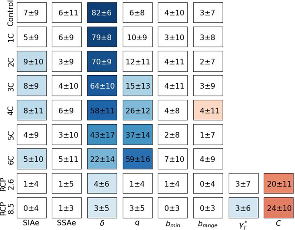
Among the ice dynamic parameters, for the low ocean warming simulations the lower limit till effective pressure as a fraction of overburden δ had the strongest influence on total sea level contribution (Fig. 11). Lower values of δ were associated with more mass loss due to the lower yield stresses. As the values of q were close to 1 in our simulations and therefore the till deformed near-linearly, the yield stress increased near-linearly with δ. Albrecht and others (Reference Albrecht, Winkelmann and Levermann2020b) suggests that values of δ should be between 0.02 and 0.1 for Antarctica, and the mode in this study was 0.85. The choice of the value of q in the sliding law has been shown to have high significance on ice loss in scenarios with retreating grounding lines and marine ice instability (Joughin and others, Reference Joughin, Smith and Schoof2019), and we found q to be the most important parameter in the scenarios with the highest ocean temperatures and largest grounding line retreats. Our values of q were near linear (q = 1) while Joughin and others (Reference Joughin, Smith and Schoof2019) suggest applying coulomb flow (q = 0), but we both found that lower values of q result in higher mass loss in these situations. Spatially, the lowest variability in ice velocity between ensemble members relative to mean velocity occurred on ice shelves and near grounding lines.
Some of the calibrated parameter values are centered on values that vary from previous literature, although this is likely the result of running PISM in a regional setup. The SIAe factor is centered around 1.0 (Fig. 3 and S1), which is below its expected value of 4–6 (Ma and others, Reference Ma2010), and SSAe here is centered around 1.3, which is well above it's expected value of below 1 for ice stream/plug flow (Ma and others, Reference Ma2010). It has been our experience that at higher resolutions, PISM provides a lower misfit to observed velocities with lower values of SIAe. The high value of SSAe in this case is likely related to the fact that this region contains a large number of ice streams and area of floating ice. These values differ from laboratory experiments, yet in ice sheet modeling the enhancement factors are often used to capture unresolved effects. The parameter tuning aims to best capture the surface speeds of ice with the goal of providing more realistic simulations of the region under a model of known ice physics.
5. Conclusion
The Filchner-Ronne region has likely experienced small mass gains in recent decades (Shepherd and others, Reference Shepherd2018; Zwally and others, Reference Zwally, Robbins, Luthcke, Loomis and Rémy2021), and the results presented here demonstrate the region continuing to experience small mass gains when applying surface and ocean forcing from RCP 2.6 and 8.5 emission scenarios to an ensemble of ice sheet model simulations. The modeled mass gains at 2100 result in a sea level reduction of 24±7 mm compared to 2015 for RCP 2.6 and 28±9 mm for RCP 8.5. The greater mass gains of RCP 8.5 were primarily driven by increased accumulation anomalies at low surface elevations in the NorESM, CCSM4, and MIROC-ESM-CHEM climate forcing. These climatic mass balance anomalies resulted in an additional 52 Gt a−1 in 2090–2100 compared to 2015–2025, or a spatially averaged elevation change of 0.02 m a−1, and balanced out the increasing basal mass loss. We used MCMC sampling of a surrogate model to optimize model parameter values and reduce projection uncertainty due to dynamic parameters.
Ocean warming in the Filchner-Ronne region is associated with decreased ice mass, greater sea level contributions, higher grounding line fluxes, and increased grounding line retreat. We found that between 2015 and 2100 this region contributes an additional 11 mm of sea level rise with one degree of ocean warming above present, and the rate of mass loss with ocean temperature increases at higher temperatures. With increasing ocean temperatures we find grounding line retreat along virtually all ice streams, resulting in 23 200 km2 less grounded area at 2100 per degree of ocean warming.
Supplementary material
The supplementary material for this article can be found at https://doi.org/10.1017/jog.2023.10.
Acknowledgements
Andrew Johnson was supported by NSF Award #1543432 and the Alaska Satellite Facility. Torsten Albrecht was supported by the Deutsche Forschungsgemeinschaft (DFG) in the framework of the priority program “Antarctic Research with comparative investigations in Arctic ice areas” by grants WI4556/2-1, and within the framework of the PalMod project (FKZ: 01LP1925D) supported by the German Federal Ministry of Education and Research (BMBF) as a Research for Sustainability initiative (FONA). Development of PISM is supported by NASA grants 20-CRYO2020-0052 and 80NSSC22K0274 and NSF grants PLR 1914668 and OAC-2118285. We are thankful to Melchior van Wessem for providing climatic forcing data from RACMO2.3p2 and to R. Timmermann for providing the FESOM ocean model data. We are also grateful to Constantine Khroulev for providing technical assistance with PISM.


 Open access