








1 Introduction
1.1 Discrete Chebyshev system
Let $C[a,b]$
be the space of continuous real-valued functions on a finite interval
$C[a,b]$
be the space of continuous real-valued functions on a finite interval $[a,b]$
equipped with the norm
$[a,b]$
equipped with the norm $ \|f\|_{\infty }=\max _{t\in [a,b]}|f(t)|. $
Given linearly independent functions
$ \|f\|_{\infty }=\max _{t\in [a,b]}|f(t)|. $
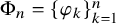
Given linearly independent functions $\{\varphi _k(t)\}_{k=1}^n\subset C[a,b]$
, the set of polynomials is defined by
$\{\varphi _k(t)\}_{k=1}^n\subset C[a,b]$
, the set of polynomials is defined by
 $$\begin{align*}L_n=\Big\{p=\sum_{k=1}^na_k\varphi_k\colon a_k\in\mathbb{R}\Big\}. \end{align*}$$
The best approximation of a continuous function f by $L_n$
is given by
$L_n$
is given by
 $$ \begin{align*} E(f,L_n)_{\infty}=\min_{p\in L_n}\|f-p\|_{\infty}=\|f-p^{*}\|_{\infty} \end{align*} $$
and $p^{*}\in L_n$
is the best approximant.
$p^{*}\in L_n$
is the best approximant.
The Chebyshev systems play the key role in a study of the best approximation of continuous functions by the n-dimensional subsets. Recall that a set of continuous functions $\{\varphi _k\}_{k=1}^n$
is called a T-system (or a Chebyshev system) on
$\{\varphi _k\}_{k=1}^n$
is called a T-system (or a Chebyshev system) on $[a,b]$
if any nontrivial polynomial with respect to this system has at most
$[a,b]$
if any nontrivial polynomial with respect to this system has at most $n-1$
distinct zeros on
$n-1$
distinct zeros on $[a,b]$
. This definition can be equivalently written as follows (cf. [Reference Karlin and Studden21, Ch. 1, § 4]): The set
$[a,b]$
. This definition can be equivalently written as follows (cf. [Reference Karlin and Studden21, Ch. 1, § 4]): The set $\{\varphi _k\}_{k=1}^n$
is a T-system if and only if, for any sequence
$\{\varphi _k\}_{k=1}^n$
is a T-system if and only if, for any sequence $a\le t_1<\dots <t_n\le b$
, the determinants
$a\le t_1<\dots <t_n\le b$
, the determinants

have the same sign.
Let us recall two crucial facts on the best approximations in $C[a,b]$
.
$C[a,b]$
.
Haar’s theorem [Reference Laurent24, Th. 3.4.6]
The best approximant $p^{*}\in L_n$
of a function
$p^{*}\in L_n$
of a function $f\in C[a,b]$
is unique if and only if
$f\in C[a,b]$
is unique if and only if $\{\varphi _k\}_{k=1}^{n}\subset C[a,b]$
is a Chebyshev system.
$\{\varphi _k\}_{k=1}^{n}\subset C[a,b]$
is a Chebyshev system.
Chebyshev’s theorem [Reference Laurent24, Th. 3.4.7]
Let $\{\varphi _k\}_{k=1}^{n}\subset C[a,b]$
be the Chebyshev system. A polynomial
$\{\varphi _k\}_{k=1}^{n}\subset C[a,b]$
be the Chebyshev system. A polynomial $p^{*}\in L_n$
is the best approximant of a function
$p^{*}\in L_n$
is the best approximant of a function $f\in C[a,b]$
if and only if there exists an ordered set of
$f\in C[a,b]$
if and only if there exists an ordered set of $n+1$
points
$n+1$
points $a\le t_1<\dots <t_{n+1}\le b$
such that
$a\le t_1<\dots <t_{n+1}\le b$
such that
 $$ \begin{align} \begin{aligned} \text{(i)}&\quad |p^{*}(t_i)-f(t_i)|=\|p^{*}-f\|_{\infty},\quad i=1,\dots,n+1,\qquad \\ \text{(ii)}&\quad p^{*}(t_i)-f(t_i)=-(p^{*}(t_{i+1})-f(t_{i+1})),\quad i=1,\dots,n. \end{aligned} \end{align} $$
Recall that an ordered set of $\{t_i\}$
satisfying properties (1.2) is called the Chebyshev alternance set of length
$\{t_i\}$
satisfying properties (1.2) is called the Chebyshev alternance set of length $n+1$
.
$n+1$
.
We are interested in analogues of Haar’s and Chebyshev’s theorems for the best uniform approximation of discrete functions defined on ordered sets of points, rather than on an interval. Note that some basic results can be partially derived from well-known results on the best uniform approximation of continuous functions on an arbitrary compact set (see, e.g., [Reference Dunham11], [Reference Dzyadyk and Shevchuk12, Ch. 1, §§ 2, 5], [Reference Gantmacher and Krein15, Ch. II], [Reference Laurent24, Ch. 3]).
For $m,n\in \mathbb {Z}$
,
$m,n\in \mathbb {Z}$
, $m\le n$
, we define
$m\le n$
, we define $[m,n]_{{\scriptscriptstyle \mathbb {Z}}}=\{m,m+1,\dots ,n\}$
. For
$[m,n]_{{\scriptscriptstyle \mathbb {Z}}}=\{m,m+1,\dots ,n\}$
. For $q\in \mathbb {N}$
, letFootnote
1
$q\in \mathbb {N}$
, letFootnote
1 $C[0,q]_{{\scriptscriptstyle \mathbb {Z}}}=\{f\colon [0,q]_{{\scriptscriptstyle \mathbb {Z}}}\to \mathbb {R}\}$
be the linear space (of the dimension
$C[0,q]_{{\scriptscriptstyle \mathbb {Z}}}=\{f\colon [0,q]_{{\scriptscriptstyle \mathbb {Z}}}\to \mathbb {R}\}$
be the linear space (of the dimension $q+1$
) of real-valued discrete functions on
$q+1$
) of real-valued discrete functions on $[0,q]_{{\scriptscriptstyle \mathbb {Z}}}$
equipped with the norm
$[0,q]_{{\scriptscriptstyle \mathbb {Z}}}$
equipped with the norm $ \|f\|_{\infty }=\max _{\nu \in [0,q]_{{\scriptscriptstyle \mathbb {Z}}}}|f(\nu )|. $
The point
$ \|f\|_{\infty }=\max _{\nu \in [0,q]_{{\scriptscriptstyle \mathbb {Z}}}}|f(\nu )|. $
The point $\nu $
is called a zero of the discrete function f ifFootnote
2
either
$\nu $
is called a zero of the discrete function f ifFootnote
2
either
 $$\begin{align*}f(\nu)=0\ \ \text{for}\ \ \nu \in [0,q]_{{\scriptscriptstyle\mathbb{Z}}} \quad \text{or}\quad f(\nu-1)f(\nu)<0\ \ \text{for}\ \ \nu \in [1,q]_{{\scriptscriptstyle\mathbb{Z}}}. \end{align*}$$
It will be important to distinguish these zeros and we will call them the zeros of the first or second type, respectively. Denote by $N(f,[m,n]_{{\scriptscriptstyle \mathbb {Z}}})$
the number of zeros (of both types) of f on
$N(f,[m,n]_{{\scriptscriptstyle \mathbb {Z}}})$
the number of zeros (of both types) of f on $[m,n]_{{\scriptscriptstyle \mathbb {Z}}}$
. Set also
$[m,n]_{{\scriptscriptstyle \mathbb {Z}}}$
. Set also $N(f)=N(f,[0,q]_{{\scriptscriptstyle \mathbb {Z}}})$
. Moreover, let
$N(f)=N(f,[0,q]_{{\scriptscriptstyle \mathbb {Z}}})$
. Moreover, let $N_0(f)$
be the number of zeros of the first type of f on
$N_0(f)$
be the number of zeros of the first type of f on $[0,q]_{{\scriptscriptstyle \mathbb {Z}}}$
. Clearly,
$[0,q]_{{\scriptscriptstyle \mathbb {Z}}}$
. Clearly, $N_{0}(f)\le N(f)$
.
$N_{0}(f)\le N(f)$
.
F. Gantmacher and M. Krein [Reference Gantmacher and Krein15, Ch. II] suggested the following characteristics of oscillatory properties of discrete functions. Let $S^{-}(f)$
(respectively,
$S^{-}(f)$
(respectively, $S^{+}(f)$
) be the least (the largest) number of sign changesFootnote
3
of f on
$S^{+}(f)$
) be the least (the largest) number of sign changesFootnote
3
of f on $[0,q]_{{\scriptscriptstyle \mathbb {Z}}}$
after replacing all zero values of f by arbitrary nonzero values. We claim that
$[0,q]_{{\scriptscriptstyle \mathbb {Z}}}$
after replacing all zero values of f by arbitrary nonzero values. We claim that
 $$\begin{align*}S^{-}(f)\le N(f)\le S^{+}(f), \end{align*}$$
with the discussion and proof given in Section 3 (see Lemma 3.1).
We study the problem of the characterization and uniqueness of the best uniform approximants of discrete functions. Let $\{\varphi _k\}_{k=1}^{n}\subset C[0,q]_{{\scriptscriptstyle \mathbb {Z}}}$
be linearly independent discrete functions and
$\{\varphi _k\}_{k=1}^{n}\subset C[0,q]_{{\scriptscriptstyle \mathbb {Z}}}$
be linearly independent discrete functions and $L_n$
be its linear span over
$L_n$
be its linear span over $\mathbb {R}$
. As in the continuous case,
$\mathbb {R}$
. As in the continuous case,
 $$\begin{align*}E(f,L_n)_{\infty}=\min_{p\in L_n}\|f-p\|_{\infty}=\|f-p^{*}\|_{\infty} \end{align*}$$
is the best uniform approximation of f by $L_n$
and
$L_n$
and $p^{*}\in L_n$
is the best approximant.
$p^{*}\in L_n$
is the best approximant.
Since, for discrete functions one can distinguish between two types of zeros, we define two corresponding discrete Chebyshev systems. Let $n\in [1,q+1]_{{\scriptscriptstyle \mathbb {Z}}}$
. The set of discrete functions
$n\in [1,q+1]_{{\scriptscriptstyle \mathbb {Z}}}$
. The set of discrete functions $\{\varphi _k\}_{k=1}^{n}\subset C[0,q]_{{\scriptscriptstyle \mathbb {Z}}}$
is called the
$\{\varphi _k\}_{k=1}^{n}\subset C[0,q]_{{\scriptscriptstyle \mathbb {Z}}}$
is called the $T_{{\scriptscriptstyle \mathbb {Z}}}$
-system (respectively,
$T_{{\scriptscriptstyle \mathbb {Z}}}$
-system (respectively, $T_{0}$
-system) if for any nontrivial polynomial
$T_{0}$
-system) if for any nontrivial polynomial
 $$ \begin{align} p(\nu)=\sum_{k=1}^{n}a_k\varphi_k(\nu) \end{align} $$
of degree at most n with real coefficients we have $N(p)\le n-1$
(
$N(p)\le n-1$
( $N_0(p)\le n-1$
). It is clear that any
$N_0(p)\le n-1$
). It is clear that any $T_{{\scriptscriptstyle \mathbb {Z}}}$
-system is also
$T_{{\scriptscriptstyle \mathbb {Z}}}$
-system is also $T_0$
-system but the inverse statement is not valid, see the example in Section 2.
$T_0$
-system but the inverse statement is not valid, see the example in Section 2.
Let $p^{*}\in L_n$
be the best uniform approximant of the function
$p^{*}\in L_n$
be the best uniform approximant of the function $f\in C[0,q]_{{\scriptscriptstyle \mathbb {Z}}}$
and set
$f\in C[0,q]_{{\scriptscriptstyle \mathbb {Z}}}$
and set
 $$\begin{align*}e(\nu)=p^{*}(\nu)-f(\nu), \quad \nu \in [0,q]_{{\scriptscriptstyle\mathbb{Z}}}. \end{align*}$$
Due to compactness of $[0,q]_{{\scriptscriptstyle \mathbb {Z}}}\subset \mathbb {R}$
, we observe that an analogue of Haar’s theorem is valid only for
$[0,q]_{{\scriptscriptstyle \mathbb {Z}}}\subset \mathbb {R}$
, we observe that an analogue of Haar’s theorem is valid only for $T_0$
-systems.
$T_0$
-systems.
Theorem 1.1 [Reference Laurent24, Th. 3.4.6]
The best uniform approximant $p^*\in L_n$
of the function
$p^*\in L_n$
of the function $f\in C[0,q]_{{\scriptscriptstyle \mathbb {Z}}}$
is unique if and only if the set
$f\in C[0,q]_{{\scriptscriptstyle \mathbb {Z}}}$
is unique if and only if the set $\{\varphi _k\}_{k=1}^{n}\subset C[0,q]_{{\scriptscriptstyle \mathbb {Z}}}$
is a
$\{\varphi _k\}_{k=1}^{n}\subset C[0,q]_{{\scriptscriptstyle \mathbb {Z}}}$
is a $T_0$
-system.
$T_0$
-system.
We note that a (nontrivial) polynomial (1.3) vanishes at n integer points $0\le \nu _1<\dots <\nu _n\le q$
if and only if the determinant
$0\le \nu _1<\dots <\nu _n\le q$
if and only if the determinant
 $$ \begin{align} \Delta\left( \begin{matrix} \varphi_1, & \varphi_2, & \dots, & \varphi_n\\ \nu_1, & \nu_2, & \dots, & \nu_n \end{matrix}\right) \end{align} $$
defined by (1.1) is zero. Therefore, we arrive at the following obvious statement, which provides a criterion for $T_0$
-systems (see, e.g., [Reference Karlin and Studden21, Ch. VII, § 1]).
$T_0$
-systems (see, e.g., [Reference Karlin and Studden21, Ch. VII, § 1]).
Proposition 1.2. The set $\{\varphi _k\}_{k=1}^{n}\subset C[0,q]_{{\scriptscriptstyle \mathbb {Z}}}$
is a
$\{\varphi _k\}_{k=1}^{n}\subset C[0,q]_{{\scriptscriptstyle \mathbb {Z}}}$
is a $T_0$
-system if and only if the determinants (1.4) are nonzero for any integers
$T_0$
-system if and only if the determinants (1.4) are nonzero for any integers $0\le \nu _1<\dots <\nu _n\le q$
.
$0\le \nu _1<\dots <\nu _n\le q$
.
A straightforward analogue of Chebyshev’s theorem for $T_0$
-systems reads as follows.
$T_0$
-systems reads as follows.
Theorem 1.3 [Reference Laurent24, Th. 3.4.7]
Let the set $\{\varphi _k\}_{k=1}^{n}\subset C[0,q]_{{\scriptscriptstyle \mathbb {Z}}}$
be a
$\{\varphi _k\}_{k=1}^{n}\subset C[0,q]_{{\scriptscriptstyle \mathbb {Z}}}$
be a $T_0$
-system. The polynomial
$T_0$
-system. The polynomial $p^{*}\in L_n$
is the best uniform approximant of a function
$p^{*}\in L_n$
is the best uniform approximant of a function $f\in C[0,q]_{{\scriptscriptstyle \mathbb {Z}}}$
if and only if there exist distinct points
$f\in C[0,q]_{{\scriptscriptstyle \mathbb {Z}}}$
if and only if there exist distinct points $\nu _1, \dots ,\nu _{n+1}\in [0,q]_{{\scriptscriptstyle \mathbb {Z}}}$
,
$\nu _1, \dots ,\nu _{n+1}\in [0,q]_{{\scriptscriptstyle \mathbb {Z}}}$
, $\varepsilon _1,\ldots ,\varepsilon _{n+1}\in \{-1,1\}$
, and positive numbers
$\varepsilon _1,\ldots ,\varepsilon _{n+1}\in \{-1,1\}$
, and positive numbers $\rho _1,\ldots ,\rho _{n+1}$
, satisfying the conditions
$\rho _1,\ldots ,\rho _{n+1}$
, satisfying the conditions
 $$ \begin{align*} \begin{aligned} \mathrm{(i)}&\quad \varepsilon_i e(\nu_i)=\|e\|_{\infty},\quad i=1,\dots,n+1,\quad e=p^{*}-f,\\ \mathrm{(ii)}&\quad \sum_{i=1}^{n+1}\varepsilon_i\rho_i p(\nu_i)=0\quad \text{for all}\quad p\in L_n. \end{aligned} \end{align*} $$
We note that the set of points $\nu _1,\dots ,\nu _{n+1}$
in Theorem 1.3 may not form the Chebyshev alternance set as we will see in Example 2.7.
$\nu _1,\dots ,\nu _{n+1}$
in Theorem 1.3 may not form the Chebyshev alternance set as we will see in Example 2.7.
Our first main result provides a characterization of the discrete set $\{\varphi _k\}_{k=1}^{n}\subset C[0,q]_{{\scriptscriptstyle \mathbb {Z}}}$
such that for any
$\{\varphi _k\}_{k=1}^{n}\subset C[0,q]_{{\scriptscriptstyle \mathbb {Z}}}$
such that for any $f \in C[0,q]_{{\scriptscriptstyle \mathbb {Z}}}$
the best uniform approximant
$f \in C[0,q]_{{\scriptscriptstyle \mathbb {Z}}}$
the best uniform approximant $p^{*}\in L_n$
has an alternance set of length
$p^{*}\in L_n$
has an alternance set of length $n+1$
, that is, we obtain a complete analogue of Chebyshev’s alternance theorem.
$n+1$
, that is, we obtain a complete analogue of Chebyshev’s alternance theorem.
We say that the best uniform approximant $p^{*}\in L_n$
of f admits an alternance set
$p^{*}\in L_n$
of f admits an alternance set $0\le \nu _1<\dots <\nu _{n+1}\le q$
of length
$0\le \nu _1<\dots <\nu _{n+1}\le q$
of length $n+1$
if the following condition holds (cf. (1.2)):
$n+1$
if the following condition holds (cf. (1.2)):
 $$\begin{align*}\varepsilon(-1)^{i}e(\nu_i)=\|e\|_{\infty},\quad i=1,\dots,n+1,\quad \varepsilon=\pm 1. \end{align*}$$
Theorem 1.4. Let $n\in [1,q]_{{\scriptscriptstyle \mathbb {Z}}}$
. The following are equivalent
$n\in [1,q]_{{\scriptscriptstyle \mathbb {Z}}}$
. The following are equivalent $:$
$:$
-
(a) The set $\{\varphi _k\}_{k=1}^{n}\subset C[0,q]_{{\scriptscriptstyle \mathbb {Z}}}$
is a
$T_{{\scriptscriptstyle \mathbb {Z}}}$
-system.
$\{\varphi _k\}_{k=1}^{n}\subset C[0,q]_{{\scriptscriptstyle \mathbb {Z}}}$
is a
$T_{{\scriptscriptstyle \mathbb {Z}}}$
-system. -
(b) For any function
$f\in C[0,q]_{{\scriptscriptstyle \mathbb {Z}}}$
, the best uniform approximant
$p^{*}\in L_n$
of f admits an alternance set of length
$n+1$
. -
(c) Determinants (1.4) constructed over all sets
$0\le \nu _1<\dots <\nu _n\le q$
are nonzero and have the same sign.






Thus, an analogue of Chebyshev’s theorem holds only for $T_{{\scriptscriptstyle \mathbb {Z}}}$
-systems.
$T_{{\scriptscriptstyle \mathbb {Z}}}$
-systems.
Using Theorem 1.4, one can easily construct different examples of $T_{{\scriptscriptstyle \mathbb {Z}}}$
-systems via T-systems on an interval.
$T_{{\scriptscriptstyle \mathbb {Z}}}$
-systems via T-systems on an interval.
Corollary 1.5. If $\{\varphi _i(t)\}_{i=1}^n\subset C[0,q]$
is a T-system on
$\{\varphi _i(t)\}_{i=1}^n\subset C[0,q]$
is a T-system on $[0,q]$
, then
$[0,q]$
, then $\{\varphi _i(\nu )\}_{i=1}^n\subset C[0,q]_{{\scriptscriptstyle \mathbb {Z}}}$
is a
$\{\varphi _i(\nu )\}_{i=1}^n\subset C[0,q]_{{\scriptscriptstyle \mathbb {Z}}}$
is a $T_{{\scriptscriptstyle \mathbb {Z}}}$
-system.
$T_{{\scriptscriptstyle \mathbb {Z}}}$
-system.
Another important property of $T_{{\scriptscriptstyle \mathbb {Z}}}$
-systems is given below.
$T_{{\scriptscriptstyle \mathbb {Z}}}$
-systems is given below.
Corollary 1.6. If $\{\varphi _k\}_{k=1}^n\subset C[0,q]_{{\scriptscriptstyle \mathbb {Z}}}$
is a
$\{\varphi _k\}_{k=1}^n\subset C[0,q]_{{\scriptscriptstyle \mathbb {Z}}}$
is a $T_{{\scriptscriptstyle \mathbb {Z}}}$
-system, then for any nontrivial polynomial
$T_{{\scriptscriptstyle \mathbb {Z}}}$
-system, then for any nontrivial polynomial $p \in L_n$
we have
$p \in L_n$
we have $S^{+}(p)\le n-1$
.
$S^{+}(p)\le n-1$
.
Historical comments. S. Karlin and W.J. Studden [Reference Karlin and Studden21, Ch. VII] introduced $T_{{\scriptscriptstyle \mathbb {Z}}}$
-systems via condition (c) and showed that (c) yields (a). In the matrix form the implication
$T_{{\scriptscriptstyle \mathbb {Z}}}$
-systems via condition (c) and showed that (c) yields (a). In the matrix form the implication $\text {(b)}\Leftrightarrow \text {(c)}$
can be found in the recent paper [Reference Morozov, Zheltkov and Osinsky31]. Corollary 1.5 was given in [Reference Karlin and Studden21, Ch. VII, § 1] in the particular case when T-systems are generated by strictly total positive kernels. Also, Corollary 1.6 was proved in [Reference Karlin and Studden21, Ch. VII, § 2] using property (c) of Theorem 1.4. We will give a different proof of Corollary 1.6 based on an oscillation property of discrete polynomials (2.4).
$\text {(b)}\Leftrightarrow \text {(c)}$
can be found in the recent paper [Reference Morozov, Zheltkov and Osinsky31]. Corollary 1.5 was given in [Reference Karlin and Studden21, Ch. VII, § 1] in the particular case when T-systems are generated by strictly total positive kernels. Also, Corollary 1.6 was proved in [Reference Karlin and Studden21, Ch. VII, § 2] using property (c) of Theorem 1.4. We will give a different proof of Corollary 1.6 based on an oscillation property of discrete polynomials (2.4).
We note that the discrete Chebyshev approximation plays an important role in numerical analysis (see, e.g., [Reference Dunham11] and [Reference Morozov, Zheltkov and Osinsky31, Reference Zamarashkin, Morozov and Tyrtyshnikov38] for the best approximation by low-rank matrices). In these problems the use of effective algorithms such as the Remez algorithm is crucial. Let us mention that versions of Theorem 1.3 also allow one to construct effective algorithms for non-Chebyshev systems, see [Reference Protasov and Kamalov32]. Moreover, C. Dunham [Reference Dunham11] developed a discrete Remez algorithm based on alternance sets. Thus, Theorem 1.4 completes this study as it characterizes all systems that admit alternation.
For applications, it is important to construct various discrete Chebyshev systems. To this end, in the next section we consider the eigenfunctions of Sturm-Liouville problems.
1.2 Sturm oscillation theorem, T-systems, and orthogonal polynomials
We start with the following known fact: T-systems can be obtained using Sturm-Liouville problems. In 1836, C. Sturm proved the following remarkable result, which was obtained in the same year by J. Liouville using a different method under less restrictions. See [Reference Bérard and Helffer5, Reference Simon33, Reference Steinerberger34] for the historical comments.
Sturm’s theorem Let $\{V_{k}\}_{k=1}^{\infty }\subset C^{2}[a,b]$
be the set of eigenfunctions associated to eigenvalues
$\{V_{k}\}_{k=1}^{\infty }\subset C^{2}[a,b]$
be the set of eigenfunctions associated to eigenvalues $\rho _{1}<\rho _{2}<\dots $
of the following Sturm-Liouville problem:
$\rho _{1}<\rho _{2}<\dots $
of the following Sturm-Liouville problem:
 $$ \begin{align} \begin{gathered} (K(t)V'(t))'+(\rho G(t)-L(t))V(t)=0,\quad t\in [a,b],\\ (KV'-hV)(a)=0,\quad (KV'+HV)(b)=0, \end{gathered} \end{align} $$
where $G,K,L\in C[a,b]$
,
$G,K,L\in C[a,b]$
,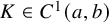 $K\in C^{1}(a,b)$
,
$K\in C^{1}(a,b)$
, $K,G>0$
on
$K,G>0$
on $(a,b)$
,
$(a,b)$
, $h,H\in [0,\infty ]$
, and
$h,H\in [0,\infty ]$
, and $\rho $
denotes the spectral parameter. Then
$\rho $
denotes the spectral parameter. Then
-
(a) Every k-th eigenfunction
$V_{k}$
has exactly
$k-1$
simple zeros in
$(a,b)$
. -
(b) For any nontrivial real polynomial of the form
(1.6)the number of distinct zeros of P on
$$ \begin{align} P(t)=\sum_{k=m}^{n}A_{k}V_{k}(t),\quad m,n\in \mathbb{N},\quad m\le n, \end{align} $$
$(a,b)$
is at least
$m-1$
and at most
$n-1$
.


Remark 1.7. (i) Part (a) is sometimes called the weak Sturm oscillation theorem [Reference Steinerberger34] and proved using comparison theorems (see, e.g., [Reference Levitan and Sargsjan26] and [Reference Simon33]). Part (b) is a much stronger result (the Sturm oscillation theorem). As noted by P. Bérard and B. Helffer [Reference Bérard and Helffer5], while part (a) is a well-known statement, part (b) has been almost forgotten. However, for the trigonometric system, it has been known since the early 20th century as the Sturm-Hurwitz theorem: If a real Fourier series has a spectral gap, that is, $f(t) = \sum _{k=m}^\infty (a_k \cos kt + b_k \sin kt)$
, then f has at least
$f(t) = \sum _{k=m}^\infty (a_k \cos kt + b_k \sin kt)$
, then f has at least $2m$
sign changes over the period. Sturm proved this fact for polynomials (cf. (1.6)), while Hurwitz extended it to the general case. Similar results on spectral gap problems are closely related to the Fourier uncertainty principle (see, e.g., [Reference Eremenko and Novikov14, Reference Gorbachev, Ivanov and Tikhonov17, Reference Gorbachev, Ivanov and Tikhonov18, Reference Logan27, Reference Mitkovski and Poltoratski29, Reference Steinerberger34, Reference Ulanovskii37]) and signal processing (see, e.g., [Reference Mao28]).
$2m$
sign changes over the period. Sturm proved this fact for polynomials (cf. (1.6)), while Hurwitz extended it to the general case. Similar results on spectral gap problems are closely related to the Fourier uncertainty principle (see, e.g., [Reference Eremenko and Novikov14, Reference Gorbachev, Ivanov and Tikhonov17, Reference Gorbachev, Ivanov and Tikhonov18, Reference Logan27, Reference Mitkovski and Poltoratski29, Reference Steinerberger34, Reference Ulanovskii37]) and signal processing (see, e.g., [Reference Mao28]).
(ii) It follows from Sturm’s theorem that $\{V_{k}(t)\}_{k=1}^{n}$
forms a T-system on the interval
$\{V_{k}(t)\}_{k=1}^{n}$
forms a T-system on the interval $(a,b)$
. By Corollary 1.5, for
$(a,b)$
. By Corollary 1.5, for $a<0$
and
$a<0$
and $b>q$
, the set
$b>q$
, the set $\{V_{k}(\nu )\}_{k=1}^{n}\subset C[0,q]_{{\scriptscriptstyle \mathbb {Z}}}$
is a
$\{V_{k}(\nu )\}_{k=1}^{n}\subset C[0,q]_{{\scriptscriptstyle \mathbb {Z}}}$
is a $T_{{\scriptscriptstyle \mathbb {Z}}}$
-system.
$T_{{\scriptscriptstyle \mathbb {Z}}}$
-system.
Our main goal in this section is to obtain the Sturm oscillation theorem for eigenfunctions of a discrete Sturm-Liouville problem on $[0,q]_{{\scriptscriptstyle \mathbb {Z}}}$
. This problem is treated in detail in several monographs, for example, [Reference Agarwal1, Ch. 12], [Reference Atkinson3, Ch. 4], [Reference Kelley and Peterson22, Ch. 7]. Moreover, discrete comparison and separation theorems in various settings have been studied in, for example, [Reference Agarwal, Bohner, Grace and O’Regan2, Reference Elaydi13, Reference Simon33, Reference Teschl36]. However, an explicit discrete analogue of Sturm’s theorem has been an open question.
$[0,q]_{{\scriptscriptstyle \mathbb {Z}}}$
. This problem is treated in detail in several monographs, for example, [Reference Agarwal1, Ch. 12], [Reference Atkinson3, Ch. 4], [Reference Kelley and Peterson22, Ch. 7]. Moreover, discrete comparison and separation theorems in various settings have been studied in, for example, [Reference Agarwal, Bohner, Grace and O’Regan2, Reference Elaydi13, Reference Simon33, Reference Teschl36]. However, an explicit discrete analogue of Sturm’s theorem has been an open question.
To formulate the discrete Sturm-Liouville problem, we use infinite tridiagonal Jacobi matrix, which is, in general, nonsymmetric. Let $\{\alpha _{l}\}_{l=0}^{\infty }$
be a sequence of real numbers,
$\{\alpha _{l}\}_{l=0}^{\infty }$
be a sequence of real numbers, $\{\gamma _{l}\}_{l=0}^{\infty }$
,
$\{\gamma _{l}\}_{l=0}^{\infty }$
, $\{\beta _{l}\}_{l=0}^{\infty }$
,
$\{\beta _{l}\}_{l=0}^{\infty }$
, $\{\rho _l\}_{l=0}^{\infty }$
be sequences of positive numbers. Define
$\{\rho _l\}_{l=0}^{\infty }$
be sequences of positive numbers. Define

Considering the eigenvalue problem
 $$ \begin{align*}JP=\lambda \rho P\end{align*} $$
with an infinite vector $P=\{P_l(\lambda )\}_{l=0}^{\infty }$
and a diagonal matrix
$P=\{P_l(\lambda )\}_{l=0}^{\infty }$
and a diagonal matrix $\rho =\operatorname {diag}(\{\rho _l\}_{l=0}^{\infty })$
, we arrive at the Sturm-Liouville problem in the recurrence relation form:
$\rho =\operatorname {diag}(\{\rho _l\}_{l=0}^{\infty })$
, we arrive at the Sturm-Liouville problem in the recurrence relation form:
 $$ \begin{align} \begin{gathered} \gamma_{l-1}P_{l-1}(\lambda)+\alpha_lP_l(\lambda)+\beta_{l}P_{l+1}(\lambda)=\lambda \rho_{l}P_l(\lambda),\quad l\in \mathbb{Z}_{+},\quad \lambda\in\mathbb{C},\\ P_{-1}(\lambda)=0,\quad P_0(\lambda)=1, \end{gathered} \end{align} $$
where $\gamma _{-1}>0$
is arbitrary. It is clear that the solution of this problem is given by a family of algebraic polynomials
$\gamma _{-1}>0$
is arbitrary. It is clear that the solution of this problem is given by a family of algebraic polynomials $P_l(\lambda )$
of degree l with positive leading coefficients.
$P_l(\lambda )$
of degree l with positive leading coefficients.
For a nondecreasing function $\mu (\lambda )$
on
$\mu (\lambda )$
on $\mathbb {R}$
, the set
$\mathbb {R}$
, the set
 $$\begin{align*}\mathcal{S}(\mu)=\{\lambda\colon \mu(\lambda+\delta)-\mu(\lambda-\delta)> 0\ \text{for all}\ \delta>0\} \end{align*}$$
is called the spectrum of $\mu $
. To attack Problem (1.7), we apply the Favard theorem (see [Reference Chihara8, Th. II. 6.4]), which leads to the following statement.
$\mu $
. To attack Problem (1.7), we apply the Favard theorem (see [Reference Chihara8, Th. II. 6.4]), which leads to the following statement.
Theorem 1.8.
-
(a) Polynomials
$P_l(\lambda )$
are orthogonal with respect to a positive measure
$\mu $
on
$\mathbb {R}$
, defined by a nondecreasing function of bounded variation with infinite spectrum, and (1.8)
$$ \begin{align} d_{l}\int_{\mathbb{R}}P_l(\lambda)P_m(\lambda)\,d\mu(\lambda)=\delta_{lm},\quad d_0=\rho_0,\quad d_l=\rho_{l}\,\frac{\beta_0\cdots \beta_{l-1}}{\gamma_0\cdots \gamma_{l-1}},\quad l\ge 1. \end{align} $$
-
(b) A measure
$\mu $
has a finite support
$[a,b]$
, the endpoints of which will be the limit points of zeros of the orthogonal polynomials
$P_l(\lambda )$
, if and only if the sequences (1.9)are bounded.
$$ \begin{align} \frac{\alpha_{l}}{\rho_{l}},\quad \frac{\gamma_{l-1}\beta_{l-1}}{\rho_{l-1}\rho_{l}} \end{align} $$


Note that positivity of coefficients $\gamma _l$
,
$\gamma _l$
, $\beta _l$
,
$\beta _l$
, $\rho _l$
is a natural condition in Theorem 1.8, see Theorem II.6.4 in [Reference Chihara8].
$\rho _l$
is a natural condition in Theorem 1.8, see Theorem II.6.4 in [Reference Chihara8].
Throughout the paper we assume that $ q\in \mathbb {Z}_+$
and
$ q\in \mathbb {Z}_+$
and $\eta \in \mathbb {R}.$
Consider the polynomial
$\eta \in \mathbb {R}.$
Consider the polynomial
 $$ \begin{align} \widetilde{P}_{q+1}(\lambda)=P_{q+1}(\lambda)-\eta P_{q}(\lambda) \end{align} $$
and define its zeros by $ \lambda _{q+1}<\dots <\lambda _{1}, $
see [Reference Szegö35, Ch. III, § 3.3]. We also define the following set of discrete functions:
$ \lambda _{q+1}<\dots <\lambda _{1}, $
see [Reference Szegö35, Ch. III, § 3.3]. We also define the following set of discrete functions:
 $$ \begin{align} \psi_k(\nu)=P_{\nu}(\lambda_k),\quad k\in [1,q+1]_{{\scriptscriptstyle\mathbb{Z}}},\quad \nu\in [0,q]_{{\scriptscriptstyle\mathbb{Z}}}. \end{align} $$
By virtue of (1.7), $\lambda _k$
and
$\lambda _k$
and $\psi _k(\nu )$
are eigenvalues and eigenfunctions of the discrete Sturm-Liouville problem
$\psi _k(\nu )$
are eigenvalues and eigenfunctions of the discrete Sturm-Liouville problem
 $$ \begin{align} \begin{gathered} \gamma_{\nu-1}\psi(\nu-1)+\alpha_{\nu}\psi(\nu)+\beta_{\nu}\psi(\nu+1)=\lambda \rho_{\nu}\psi(\nu),\quad \nu\in [0,q]_{{\scriptscriptstyle\mathbb{Z}}},\\ \psi(-1)=0,\quad \psi(0)=1,\quad \psi(q+1)=\eta\psi(q). \end{gathered} \end{align} $$
Introducing the Jacobi matrix

problem (1.12) corresponds to the eigenvalue problem
 $$ \begin{align*}J_{q+1}\psi=\lambda \rho \psi.\end{align*} $$
Sturm’s theory on the zeros of discrete polynomials with respect to the set $\{\psi _k(\nu )\}_{k=1}^{q+1}$
(see (1.11)) is similar to that in the continuous case (see (1.5)), with the additional use of the quantities
$\{\psi _k(\nu )\}_{k=1}^{q+1}$
(see (1.11)) is similar to that in the continuous case (see (1.5)), with the additional use of the quantities $S^{-}(f)$
and
$S^{-}(f)$
and $S^{+}(f)$
.
$S^{+}(f)$
.
Before stating an analogue of item (a) of Sturm’s theorem given in Theorem 1.10 below, we mention the following result by B. Simon.Footnote 4
Theorem 1.9 [Reference Simon33, Th. 2.3]
For $n\in [1,q]_{\scriptscriptstyle \mathbb {Z}},$
there holds
$n\in [1,q]_{\scriptscriptstyle \mathbb {Z}},$
there holds
 $$\begin{align*}|\{j\in [1,n]_{\scriptscriptstyle\mathbb{Z}}\colon \lambda<\lambda_{j,n}\}|= |\{\nu\in [1,n]_{\scriptscriptstyle\mathbb{Z}}\colon \operatorname{sign} P_{\nu-1}(\lambda)\ne \operatorname{sign} P_{\nu}(\lambda)\}|, \end{align*}$$
where $\lambda _{l,l}<\dots <\lambda _{1,l}$
are the zeros of the polynomials
$\lambda _{l,l}<\dots <\lambda _{1,l}$
are the zeros of the polynomials $P_l(\lambda )$
,
$P_l(\lambda )$
, $\lambda \ne \lambda _{j,l}$
for
$\lambda \ne \lambda _{j,l}$
for $1\le j\le l\le n$
, and
$1\le j\le l\le n$
, and $|I|$
denotes the cardinality of a finite set I.
$|I|$
denotes the cardinality of a finite set I.
Taking into account that the function $\psi _k$
cannot have two consecutive zeros of the first type, this theorem implies the following result.
$\psi _k$
cannot have two consecutive zeros of the first type, this theorem implies the following result.
Theorem 1.10. For all $k\in [1,q+1]_{{\scriptscriptstyle \mathbb {Z}}},$
 $$\begin{align*}S^{-}(\psi_k)=S^{+}(\psi_k)=N(\psi_k)=k-1. \end{align*}$$
Note that Theorem 1.10 also follows from Theorem 1 in [Reference Gantmacher and Krein15, Ch. II] whose proof is based on the use of the concepts of lines and nodes for the piecewise linear function associated with Jacobi matrices (see Definition 2 in [Reference Gantmacher and Krein15, Ch. II]). Moreover, the proof of the fact that $N(\psi _k)=k-1$
based on the discrete Sturm separation theorem can be found in [Reference Kelley and Peterson22, Theorem 7.6]. The corresponding results for self-adjoint systems are given in [Reference Došlý and Kratz9, Theorem 2], [Reference Došlý, Elyseeva and Hilscher10, Corollary 5.79], [Reference Kratz23, Theorem 1]. In Section 3, we present a simple proof of Theorem 1.10 based on the property of the interlacing of zeros of orthogonal polynomials (see (3.2)).
$N(\psi _k)=k-1$
based on the discrete Sturm separation theorem can be found in [Reference Kelley and Peterson22, Theorem 7.6]. The corresponding results for self-adjoint systems are given in [Reference Došlý and Kratz9, Theorem 2], [Reference Došlý, Elyseeva and Hilscher10, Corollary 5.79], [Reference Kratz23, Theorem 1]. In Section 3, we present a simple proof of Theorem 1.10 based on the property of the interlacing of zeros of orthogonal polynomials (see (3.2)).
Our main result in this section is the discrete counterpart of item (b) of Sturm’s theorem, cf. Remark 1.7.
Theorem 1.11. Let integers m and n satisfy $1\le m\le n\le q+1$
. For any nontrivial polynomial
$1\le m\le n\le q+1$
. For any nontrivial polynomial
 $$ \begin{align} V(\nu)=\sum_{k=m}^{n}a_k\psi_k(\nu), \end{align} $$
we have
 $$ \begin{align} m-1\le S^{-}(V)\le N(V)\le S^{+}(V)\le n-1. \end{align} $$
The proof of Theorem 1.11 is based on Theorem 1.10 and a generalization of Liouville’s method (see [Reference Bérard and Helffer5]). Note also that the inequalities $m-1\le S^{-}(V)$
and
$m-1\le S^{-}(V)$
and $S^{+}(V)\le n-1$
for
$S^{+}(V)\le n-1$
for $\eta =0$
and
$\eta =0$
and $\rho _l=1$
were proven in [Reference Gantmacher and Krein15, Ch. II, Th. 6] under the assumption that the Jacobi matrix
$\rho _l=1$
were proven in [Reference Gantmacher and Krein15, Ch. II, Th. 6] under the assumption that the Jacobi matrix $J_{q+1}$
is oscillatory. Recall that a square matrix is called oscillatory if it is totally non-negative, and some power of it is totally positive (see [Reference Gantmacher and Krein15, Ch. II, Definition 4]). In our case, in general, the matrix
$J_{q+1}$
is oscillatory. Recall that a square matrix is called oscillatory if it is totally non-negative, and some power of it is totally positive (see [Reference Gantmacher and Krein15, Ch. II, Definition 4]). In our case, in general, the matrix $J_{q+1}$
is not oscillatory and it becomes oscillatory only if all its principal minors are positive [Reference Gantmacher and Krein15, Ch. II, Th. 11]. It is worth mentioning that the estimate
$J_{q+1}$
is not oscillatory and it becomes oscillatory only if all its principal minors are positive [Reference Gantmacher and Krein15, Ch. II, Th. 11]. It is worth mentioning that the estimate $N(V)\le n-1$
was mentioned in [Reference Atkinson3, Problem 2, p. 539].
$N(V)\le n-1$
was mentioned in [Reference Atkinson3, Problem 2, p. 539].
Corollary 1.12. For any $n\in [1,q+1]_{{\scriptscriptstyle \mathbb {Z}}}$
, the set
$n\in [1,q+1]_{{\scriptscriptstyle \mathbb {Z}}}$
, the set $\{\psi _k(\nu )\}_{k=1}^{n}$
is a
$\{\psi _k(\nu )\}_{k=1}^{n}$
is a $T_{{\scriptscriptstyle \mathbb {Z}}}$
-system.
$T_{{\scriptscriptstyle \mathbb {Z}}}$
-system.
To conclude, we state the discrete spectral gap theorem (cf. Remark 1.7).
Corollary 1.13. Let $m\in [1,q+1]_{{\scriptscriptstyle \mathbb {Z}}}$
and
$m\in [1,q+1]_{{\scriptscriptstyle \mathbb {Z}}}$
and $f\in C[0,q]_{{\scriptscriptstyle \mathbb {Z}}}$
be such that
$f\in C[0,q]_{{\scriptscriptstyle \mathbb {Z}}}$
be such that $f(\nu )=\sum _{k=m}^{q+1}a_k\psi _k(\nu )$
. Then
$f(\nu )=\sum _{k=m}^{q+1}a_k\psi _k(\nu )$
. Then $m-1\le S^{-}(f)\le N(f)$
.
$m-1\le S^{-}(f)\le N(f)$
.
1.3 Monotonicity property of coefficients of polynomials with removed largest zeros
Consider polynomial (1.10) and divide it into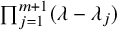 $\prod _{j=1}^{m+1} (\lambda -\lambda _{j})$
with
$\prod _{j=1}^{m+1} (\lambda -\lambda _{j})$
with $m+1$
largest zeros
$m+1$
largest zeros $\lambda _{j}$
,
$\lambda _{j}$
, $m\le q$
. Taking into account (1.8), we expand it into the Fourier sum
$m\le q$
. Taking into account (1.8), we expand it into the Fourier sum
 $$ \begin{align} \frac{\widetilde{P}_{q+1}(\lambda)}{(\lambda-\lambda_{1})\cdots (\lambda-\lambda_{m+1})}= \sum_{l=0}^{q-m}d_{l}a_{l}P_{l}(\lambda). \end{align} $$
The question arises whether all coefficients $a_{l}\ge 0$
. It turns out that the answer is affirmative. The case
$a_{l}\ge 0$
. It turns out that the answer is affirmative. The case $m=0$
is simple and corresponds to the Christoffel-Darboux formula, while the case
$m=0$
is simple and corresponds to the Christoffel-Darboux formula, while the case $m=1$
was proven in [Reference Gorbachev and Ivanov16]. In full generality, this nontrivial fact was proven by H. Cohn and A. Kumar [Reference Cohn and Kumar7, Th. 3.1] while working on the problem on discrete energy on the Euclidean sphere.
$m=1$
was proven in [Reference Gorbachev and Ivanov16]. In full generality, this nontrivial fact was proven by H. Cohn and A. Kumar [Reference Cohn and Kumar7, Th. 3.1] while working on the problem on discrete energy on the Euclidean sphere.
In this section, using the discrete Sturm theorem, we take one step further and establish the monotonicity property of the Fourier coefficients for all m, which also implies that $a_{l}\ge 0$
. This fact is crucial to deal with a spectral gap problem in Section 1.4.
$a_{l}\ge 0$
. This fact is crucial to deal with a spectral gap problem in Section 1.4.
Also, we note that the related polynomial $p_m(\lambda )=\frac {P_{q+1}^2(\lambda )}{(\lambda -\lambda _{1})\cdots (\lambda -\lambda _{m+1})}$
appeared in various extremal problems. For example, S. Bernstein used
$p_m(\lambda )=\frac {P_{q+1}^2(\lambda )}{(\lambda -\lambda _{1})\cdots (\lambda -\lambda _{m+1})}$
appeared in various extremal problems. For example, S. Bernstein used $p_0$
to disprove the existence of Chebyshev’s quadrature formula. Moreover, this polynomial is an extremizer in the following question (see [Reference Babenko4, Reference Montgomery and Ulrike30]): find
$p_0$
to disprove the existence of Chebyshev’s quadrature formula. Moreover, this polynomial is an extremizer in the following question (see [Reference Babenko4, Reference Montgomery and Ulrike30]): find
 $$ \begin{align*}\inf_{a_k, b_k} \operatorname{mes}\,\Big\{x\in (-\pi,\pi]\colon \sum_{k=1}^n (a_k\cos kx+b_k\sin kx)>0\Big\}.\end{align*} $$
V. Yudin used $p_m$
in problems of multiple covering of the torus [Reference Yudin40] and the Euclidean sphere [Reference Yudin41].
$p_m$
in problems of multiple covering of the torus [Reference Yudin40] and the Euclidean sphere [Reference Yudin41].
Our main result here is the following theorem.
Theorem 1.14. Let $q\in \mathbb {N}$
and
$q\in \mathbb {N}$
and $m\in [0,q]_{{\scriptscriptstyle \mathbb {Z}}}$
. Let also
$m\in [0,q]_{{\scriptscriptstyle \mathbb {Z}}}$
. Let also $(a,b)$
be an interval containing all the zeros of the polynomial
$(a,b)$
be an interval containing all the zeros of the polynomial $P_{q }(\lambda )$
and
$P_{q }(\lambda )$
and $\eta _{b}=P_{q+1}(b)/P_{q}(b)$
.
$\eta _{b}=P_{q+1}(b)/P_{q}(b)$
.
The following inequalities hold for the coefficients $a_l$
in the expansion (1.15)
$a_l$
in the expansion (1.15) $:$
$:$
-
(a) if either
$m\ge 1$
and
$\eta \in \mathbb {R}$
or
$m=0$
and
$\eta <\eta _{b}$
, then (1.16)
$$ \begin{align} \frac{a_0}{P_0(b)}>\frac{a_1}{P_1(b)}>\cdots>\frac{a_{q-m}}{P_{q-m}(b)}>0; \end{align} $$
-
(b) if
$m=0$
and
$\eta =\eta _{b}$
, then (1.17)
$$ \begin{align} \frac{a_0}{P_0(b)}=\frac{a_1}{P_1(b)}=\cdots=\frac{a_{q}}{P_{q}(b)}>0; \end{align} $$
-
(c) if
$m=0$
and
$\eta>\eta _b$
, then (1.18)
$$ \begin{align} 0<\frac{a_0}{P_0(b)}<\frac{a_1}{P_1(b)}<\cdots<\frac{a_{q}}{P_{q}(b)}. \end{align} $$


For polynomials normalized by $P_{l}(1)=1$
, this result has a simpler form.
$P_{l}(1)=1$
, this result has a simpler form.
Corollary 1.15. Let $P_{l}(\lambda )$
be orthogonal on
$P_{l}(\lambda )$
be orthogonal on $[-1,1]$
and
$[-1,1]$
and $P_{l}(1)=1$
. Then
$P_{l}(1)=1$
. Then
 $$\begin{align*}{\begin{cases} a_0>a_1>\cdots>a_{q-m}>0,&\text{if either } m=0 \text{ and } \eta<1 \text{ or } m\ge1 \text{ and } \eta\in\mathbb{R}, \\ a_0=a_1=\cdots=a_{q}>0,&\text{if } m=0 \text{ and } \eta=1,\\ 0<a_0<a_1<\cdots<a_{q},&\text{if } m=0 \text{ and } \eta>1. \end{cases}} \end{align*}$$
1.4 An extremal problem for polynomials with spectral gap
Let $m,n\in \mathbb {Z}_+$
,
$m,n\in \mathbb {Z}_+$
, $m<n$
. Let also
$m<n$
. Let also $\mu $
be the measure on
$\mu $
be the measure on $[-1,1]$
from Theorem 1.8 and
$[-1,1]$
from Theorem 1.8 and $\{U_{l}\}$
be the set of polynomials orthogonal on
$\{U_{l}\}$
be the set of polynomials orthogonal on $[-1,1]$
with respect to
$[-1,1]$
with respect to $d\mu $
with normalization
$d\mu $
with normalization $U_{l}(1 )=1$
,
$U_{l}(1 )=1$
, $d_l\int _{-1}^1U_lU_m\,d\mu =\delta _{lm}$
.
$d_l\int _{-1}^1U_lU_m\,d\mu =\delta _{lm}$
.
We consider the following problem: find $\lambda \in [-1,1]$
and an algebraic polynomial of degree n on
$\lambda \in [-1,1]$
and an algebraic polynomial of degree n on $[-1,1]$
with non-negative Fourier coefficients in
$[-1,1]$
with non-negative Fourier coefficients in $\{U_{l}\}$
having a spectral gap of the length m (equivalently, with the first m moments being zero), which preserves its sign over the largest possible interval
$\{U_{l}\}$
having a spectral gap of the length m (equivalently, with the first m moments being zero), which preserves its sign over the largest possible interval $[-1,\lambda ]$
.
$[-1,\lambda ]$
.
Let $\Pi $
be the set of real algebraic polynomials and
$\Pi $
be the set of real algebraic polynomials and $\Pi _n$
consist of those of degree at most n. By
$\Pi _n$
consist of those of degree at most n. By $\Pi _{+}(\{U_{l}\})$
we denote a subset of
$\Pi _{+}(\{U_{l}\})$
we denote a subset of $p\in \Pi $
such that all coefficients
$p\in \Pi $
such that all coefficients $a_{l}$
in the Fourier expansion
$a_{l}$
in the Fourier expansion
 $$ \begin{align*} p(t)=\sum_{l}d_{l}a_{l}U_{l}(t),\quad a_{l}=a_l(p)=\int_{-1}^{1}p(t)U_{l}(t)\,d\mu(t), \end{align*} $$
are non-negative.
Set
 $$ \begin{align*} K_{n}(\mu,m)=\Big\{p\in\Pi_n\cap\Pi_{+}(\{U_l\})\colon \mu_i(p)=0,\ i=0,\dots,m-1,\ \mu_{m}(p)\ge 0\Big\}, \end{align*} $$
where $\mu _i(p)=\int _{-1}^{1}t^ip(t)\,d\mu (t)$
is the ith moment of the polynomial p. Note that the conditions
$\mu _i(p)=\int _{-1}^{1}t^ip(t)\,d\mu (t)$
is the ith moment of the polynomial p. Note that the conditions $\mu _i(p)=0$
are equivalent to the fact that
$\mu _i(p)=0$
are equivalent to the fact that $a_i(p)=0$
,
$a_i(p)=0$
, $ i=0,\dots ,m-1.$
Our goal is to find the quantity
 $$\begin{align*}B_n(\mu,m)=\sup_{p\in K_{n}(\mu,m)\setminus \{0\}}\{\lambda\in [-1,1]\colon (-1)^{m-1}p(t)\ge 0,\ -1\le t\le\lambda\}. \end{align*}$$
This question turns out to play a crucial role in the study of spherical codes and designs. For $m=1$
it was posed by V. Yudin [Reference Yudin39]. Specifically, for
$m=1$
it was posed by V. Yudin [Reference Yudin39]. Specifically, for $m=1$
and
$m=1$
and $n=2q$
, he found extremizers for this problem, though the positivity of the Fourier coefficients was not proven. Further results in this direction can be found in [Reference Gorbachev and Ivanov16, Reference Gorbachev, Ivanov and Tikhonov17, Reference Gorbachev, Ivanov and Tikhonov18]; see also [Reference Cohn and Kumar7, Reference Levenshtein25].
$n=2q$
, he found extremizers for this problem, though the positivity of the Fourier coefficients was not proven. Further results in this direction can be found in [Reference Gorbachev and Ivanov16, Reference Gorbachev, Ivanov and Tikhonov17, Reference Gorbachev, Ivanov and Tikhonov18]; see also [Reference Cohn and Kumar7, Reference Levenshtein25].
Let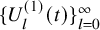 $\{U_l^{(1)}(t)\}_{l=0}^{\infty }$
be the set of polynomials with normalization
$\{U_l^{(1)}(t)\}_{l=0}^{\infty }$
be the set of polynomials with normalization $U_l^{(1)}(1) =1$
, orthogonal on
$U_l^{(1)}(1) =1$
, orthogonal on $[-1,1]$
with respect to the measure
$[-1,1]$
with respect to the measure $d\mu ^{(1)}(t)=(1+t)\,d\mu (t)$
. The zeros of the polynomials
$d\mu ^{(1)}(t)=(1+t)\,d\mu (t)$
. The zeros of the polynomials $U_{q+1}(t)$
and
$U_{q+1}(t)$
and $U_{q+1}^{(1)}(t)$
, numbered in the descending order, are denoted by
$U_{q+1}^{(1)}(t)$
, numbered in the descending order, are denoted by $t_k$
and
$t_k$
and $t_k^{(1)}$
,
$t_k^{(1)}$
, $k=1,\dots ,q+1$
, respectively.
$k=1,\dots ,q+1$
, respectively.
We say that the set of orthogonal polynomials $\{V_l\}$
satisfies the Krein property if
$\{V_l\}$
satisfies the Krein property if $V_mV_n\in \Pi _{+}(\{V_l\})$
, that is,
$V_mV_n\in \Pi _{+}(\{V_l\})$
, that is, $V_{m}V_{n}=\sum _{k=|m-n|}^{m+n}c_{m,n,k}V_{k}$
with
$V_{m}V_{n}=\sum _{k=|m-n|}^{m+n}c_{m,n,k}V_{k}$
with $c_{m,n,k}\ge 0$
, for any
$c_{m,n,k}\ge 0$
, for any $m,n\in \mathbb {Z}_+$
, see [Reference Levenshtein25].
$m,n\in \mathbb {Z}_+$
, see [Reference Levenshtein25].
Theorem 1.16. Let $m\le q$
and the set
$m\le q$
and the set $\{U_l\}$
satisfy the Krein property.
$\{U_l\}$
satisfy the Krein property.
-
(a) If
$n=2q-m+1$
, then (1.19)and the unique extremal polynomial has the form (up to a positive constant)
$$ \begin{align} B_n(\mu,m)=t_{m+1} \end{align} $$
(1.20)
$$ \begin{align} p_{n,1}^{*}(t)=\frac{U_{q+1}^2(t)}{(t-t_{1})\cdots(t-t_{m+1})}. \end{align} $$
-
(b) If
$n=2q-m+2$
and either the set
$\{U_l^{(1)}\}$
satisfies the Krein property or
$\mu (t)$
is an odd function, then (1.21)and the unique extremal polynomial has the form (up to a positive constant)
$$ \begin{align} B_n(\mu,m)=t_{m+1}^{(1)} \end{align} $$
(1.22)
$$ \begin{align} p_{n,2}^{*}(t)=\frac{(1+t)(U_{q+1}^{(1)}(t))^2}{(t-t_{1}^{(1)})\cdots(t-t_{m+1}^{(1)})}. \end{align} $$
Moreover, we have
$\mu _{m}(p_{n,j}^{*})=a_m(p_{n,j}^{*})=0$
,
$j=1,2$
.








We note that a version of Yudin-type problem for a wider class of polynomials p (without the condition $p\in \Pi _{+}(\{U_l\})$
) was solved in [Reference Ivanov20]. Our proof of Theorem 1.16 is based on Corollary 1.15.
$p\in \Pi _{+}(\{U_l\})$
) was solved in [Reference Ivanov20]. Our proof of Theorem 1.16 is based on Corollary 1.15.
1.5 Structure of the paper
The rest of the paper is organized as follows. In Section 2, we provide the proofs of Chebyshev’s theorem for $T_{{\scriptscriptstyle \mathbb {Z}}}$
-systems (Theorem 1.4) and the important Corollary 1.6, which claims that
$T_{{\scriptscriptstyle \mathbb {Z}}}$
-systems (Theorem 1.4) and the important Corollary 1.6, which claims that $S^{+}(p)\le n-1$
for a polynomial
$S^{+}(p)\le n-1$
for a polynomial $p \in L_n$
, where
$p \in L_n$
, where $p(\nu )=\sum _{k=1}^{n}a_k\varphi _k(\nu )$
and
$p(\nu )=\sum _{k=1}^{n}a_k\varphi _k(\nu )$
and $\{\varphi _k\}_{k=1}^n\subset C[0,q]_{{\scriptscriptstyle \mathbb {Z}}}$
is a
$\{\varphi _k\}_{k=1}^n\subset C[0,q]_{{\scriptscriptstyle \mathbb {Z}}}$
is a $T_{{\scriptscriptstyle \mathbb {Z}}}$
-system.
$T_{{\scriptscriptstyle \mathbb {Z}}}$
-system.
In Section 3, we study the discrete Sturm oscillation theory and its connection with T-systems and prove Theorems 1.8, 1.10, and 1.11.
Section 4 is devoted to the proof of Theorem 1.14. In Section 5, we study polynomials with spectral gaps and solve Yudin’s extremal problem (Theorem 1.16).
In the Appendix, we explicitly compute the determinants (4.1) for the Jacobi polynomials corresponding to the classical trigonometric systems. In particular, we verify that, for all $\nu \in [0,q]_{{\scriptscriptstyle \mathbb {Z}}}$
and
$\nu \in [0,q]_{{\scriptscriptstyle \mathbb {Z}}}$
and $T_{{\scriptscriptstyle \mathbb {Z}}}$
-systems,
$T_{{\scriptscriptstyle \mathbb {Z}}}$
-systems,
 $$ \begin{align*}\operatorname{sign} \Delta\left( \begin{matrix} \varphi_1, & \dots, &\varphi_{m},& \varphi_{m+1}\\ \nu_{m}, & \dots, &\nu_1, &\nu \end{matrix}\right) =\operatorname{sign} \Delta\left( \begin{matrix} \varphi_1, & \dots, &\varphi_{m},& \varphi_{m+1}\\ q, & \dots, &q-m+1, &0 \end{matrix}\right) \operatorname{sign} \prod_{j=1}^{m}(\nu_j-\nu), \end{align*} $$
which in the general case will be shown in Lemma 4.1.
2 Proofs of Theorem 1.4 and Corollary 1.6
Recall that $q\in \mathbb {Z}_+$
and
$q\in \mathbb {Z}_+$
and $\eta \in \mathbb {R}$
. The proof of Theorem 1.4 is based on Lemmas 2.1–2.5 below. First, in addition to the characteristic property of
$\eta \in \mathbb {R}$
. The proof of Theorem 1.4 is based on Lemmas 2.1–2.5 below. First, in addition to the characteristic property of $T_0$
-systems given by Proposition 1.2, we present another necessary and sufficient condition.
$T_0$
-systems given by Proposition 1.2, we present another necessary and sufficient condition.
Lemma 2.1 [Reference Laurent24, Proposition 3.4.2]
A set $\{\varphi _k\}_{k=1}^{n}\subset C[0,q]_{{\scriptscriptstyle \mathbb {Z}}}$
is a
$\{\varphi _k\}_{k=1}^{n}\subset C[0,q]_{{\scriptscriptstyle \mathbb {Z}}}$
is a $T_0$
-system if and only if, for any integers
$T_0$
-system if and only if, for any integers $0\le \nu _1<\dots <\nu _n\le q$
and any points
$0\le \nu _1<\dots <\nu _n\le q$
and any points $\{y_i\}_{i=1}^n\subset \mathbb {R}$
, there is a unique polynomial (1.3), for which
$\{y_i\}_{i=1}^n\subset \mathbb {R}$
, there is a unique polynomial (1.3), for which
 $$\begin{align*}p(\nu_i)=y_i,\quad i=1,\dots,n. \end{align*}$$
Second, we assume that the set $\{\varphi _k\}_{k=1}^{n} \subset C[0,q]_{{\scriptscriptstyle \mathbb {Z}}}$
is a
$\{\varphi _k\}_{k=1}^{n} \subset C[0,q]_{{\scriptscriptstyle \mathbb {Z}}}$
is a $T_0$
-system and the determinants (1.4) are nonzero for any integers
$T_0$
-system and the determinants (1.4) are nonzero for any integers $0 \leq \nu _1 < \dots < \nu _n \leq q$
.
$0 \leq \nu _1 < \dots < \nu _n \leq q$
.
Set, for $0\le \nu _1<\dots <\nu _{n+1}\le q$
,
$0\le \nu _1<\dots <\nu _{n+1}\le q$
,
 $$ \begin{align*} \Delta_{\nu_1}&=\Delta\left(\begin{matrix} \varphi_1,&\dots,&\varphi_n\\ \nu_2,&\dots,&\nu_{n+1} \end{matrix}\right),\quad \Delta_{\nu_{n+1}}=\Delta\left( \begin{matrix} \varphi_1,&\dots,&\varphi_n\\ \nu_1,&\dots,&\nu_{n} \end{matrix}\right), \\ \Delta_{\nu_i}&=\Delta\left( \begin{matrix} \varphi_1,&\dots,& \varphi_{i-1},& \varphi_{i},&\dots,& \varphi_n\\ \nu_1,&\dots,&\nu_{i-1},&\nu_{i+1},&\dots,& \nu_{n+1} \end{matrix}\right), \quad i=2,\dots,n. \end{align*} $$
Lemma 2.2. Let $0\le \nu _1<\dots <\nu _{n+1}\le q$
. The linear functional
$0\le \nu _1<\dots <\nu _{n+1}\le q$
. The linear functional
 $$ \begin{align} l(p)=\sum_{i=1}^{n+1}\gamma_{i}p(\nu_i)=0 \end{align} $$
for any polynomial $p\in L_n$
if and only if, up to a nonzero constant,
$p\in L_n$
if and only if, up to a nonzero constant, $\gamma _{i}=(-1)^i\Delta _{\nu _i}$
,
$\gamma _{i}=(-1)^i\Delta _{\nu _i}$
, $i=1,\dots ,n+1$
.
$i=1,\dots ,n+1$
.
Proof. First, we note that $p\in L_n$
only if
$p\in L_n$
only if
 $$\begin{align*}\Delta\left( \begin{matrix} p,&\varphi_1, & \varphi_2, & \dots, & \varphi_n\\ \nu_1,&\nu_2, & \nu_3, & \dots, & \nu_{n+1} \end{matrix}\right) =0. \end{align*}$$
Expanding the determinant along the first column, we obtain
 $$ \begin{align} \sum_{i=1}^{n+1}(-1)^{i}\Delta_{\nu_i}p(\nu_i)=0. \end{align} $$
On the other hand, from (2.1), for any $a_1,\dots ,a_k$
,
$a_1,\dots ,a_k$
,
 $$\begin{align*}0=\sum_{i=1}^{n+1}\gamma_i\sum_{k=1}^{n}a_k\varphi_k(\nu_i)=\sum_{k=1}^{n}a_k\sum_{i=1}^{n+1}\gamma_i\varphi_k(\nu_i), \end{align*}$$
and therefore,
 $$ \begin{align} \sum_{i=1}^{n+1}\gamma_i\varphi_k(\nu_i)=0,\quad k=1,\dots,n. \end{align} $$
Since $\Delta _{\nu _i}\neq 0$
, all the solutions
$\Delta _{\nu _i}\neq 0$
, all the solutions $(\gamma _1,\dots ,\gamma _{n+1})$
of the system (2.3) form a one-dimensional space. Taking into account (2.2), we arrive at the statement of the lemma.
$(\gamma _1,\dots ,\gamma _{n+1})$
of the system (2.3) form a one-dimensional space. Taking into account (2.2), we arrive at the statement of the lemma.
Lemma 2.3. Let the set $\{\varphi _k\}_{k=1}^{n}\subset C[0,q]_{{\scriptscriptstyle \mathbb {Z}}}$
be a
$\{\varphi _k\}_{k=1}^{n}\subset C[0,q]_{{\scriptscriptstyle \mathbb {Z}}}$
be a $T_{{\scriptscriptstyle \mathbb {Z}}}$
-system. The polynomial
$T_{{\scriptscriptstyle \mathbb {Z}}}$
-system. The polynomial $p^{*}\in L_n$
is the best uniform approximant of a function
$p^{*}\in L_n$
is the best uniform approximant of a function $f\in C[0,q]_{{\scriptscriptstyle \mathbb {Z}}}$
if and only if
$f\in C[0,q]_{{\scriptscriptstyle \mathbb {Z}}}$
if and only if $p^{*}$
admits an alternance set of length
$p^{*}$
admits an alternance set of length $n+1$
.
$n+1$
.
Proof. The sufficiency follows from Theorem 1.3. To prove the necessity, according to Lemma 2.2 and Theorem 1.3, we need to show that for a linear functional $l(p)$
on
$l(p)$
on $L_n$
satisfying property (2.1), there holds
$L_n$
satisfying property (2.1), there holds $\gamma _i\gamma _{i+1}<0$
for
$\gamma _i\gamma _{i+1}<0$
for $i=1,\dots ,n$
. We will follow the reasoning given in the proof of Proposition 3.5.1 in [Reference Laurent24]. Applying Lemma 2.1, we construct polynomials
$i=1,\dots ,n$
. We will follow the reasoning given in the proof of Proposition 3.5.1 in [Reference Laurent24]. Applying Lemma 2.1, we construct polynomials $p_i\in L_n$
satisfying
$p_i\in L_n$
satisfying
 $$\begin{align*}p_i(\nu_j)=0,\quad j=1,\dots,i-1, i+2,\dots,n+1,\quad p_i(\nu_i)=1. \end{align*}$$
Since $p_i$
has
$p_i$
has $n-1$
zeros of the first type, it follows from the definition of the
$n-1$
zeros of the first type, it follows from the definition of the $T_{{\scriptscriptstyle \mathbb {Z}}}$
-system that
$T_{{\scriptscriptstyle \mathbb {Z}}}$
-system that $p_i$
has no zeros of the second type and, therefore,
$p_i$
has no zeros of the second type and, therefore, $p_i( \nu _{i+1})>0$
. From this,
$p_i( \nu _{i+1})>0$
. From this,
 $$\begin{align*}l(p_i)=\gamma_ip_i(\nu_i)+\gamma_{i+1}p_{i}(\nu_{i+1})=0\quad \text{and}\quad \gamma_i\gamma_{i+1}<0, \end{align*}$$
completing the proof.
Lemma 2.4.
(a) For any $f\in C[0,q]_{{\scriptscriptstyle \mathbb {Z}}}$
, its best uniform approximant
$f\in C[0,q]_{{\scriptscriptstyle \mathbb {Z}}}$
, its best uniform approximant $p^*\in L_n$
admits an alternance set of length
$p^*\in L_n$
admits an alternance set of length $n+1$
if and only if all determinants (1.4), constructed over all sequences
$n+1$
if and only if all determinants (1.4), constructed over all sequences $0\le \nu _1<\dots <\nu _{n}\le q$
, have the same sign.
$0\le \nu _1<\dots <\nu _{n}\le q$
, have the same sign.
(b) If all determinants (1.4) have the same sign, then any sequence $0\le \nu _1<\dots <\nu _{n+1}\le q$
is an alternance set of length
$0\le \nu _1<\dots <\nu _{n+1}\le q$
is an alternance set of length $n+1$
for the polynomial
$n+1$
for the polynomial $p^*\in L_n$
, which is the best approximant of some function
$p^*\in L_n$
, which is the best approximant of some function $f\in C[0,q]_{{\scriptscriptstyle \mathbb {Z}}}$
.
$f\in C[0,q]_{{\scriptscriptstyle \mathbb {Z}}}$
.
Proof. Part (a) follows from Theorem 1.3 and Lemma 2.2.
To obtain part (b), the sequence $0\le \nu _1<\dots <\nu _{n+1}\le q$
is an alternance set of length
$0\le \nu _1<\dots <\nu _{n+1}\le q$
is an alternance set of length $n+1$
, for example, for the function
$n+1$
, for example, for the function
 $$\begin{align*}f(\nu)= \begin{cases} (-1)^{i-1},&\nu=\nu_{i},\ i=1,\dots,n+1,\\ 0&\text{otherwise}. \end{cases} \end{align*}$$
Note that, by virtue of Theorem 1.3, the best uniform approximant is $p^*(\nu )\equiv 0$
, and
$p^*(\nu )\equiv 0$
, and $E(f,L_n)_{\infty }=1$
. The proof is now complete.
$E(f,L_n)_{\infty }=1$
. The proof is now complete.
Lemma 2.5. Let $p\in L_n$
and
$p\in L_n$
and $N(p)=n$
. There exists a collection of points
$N(p)=n$
. There exists a collection of points $\Omega =\{0\le \nu _1<\dots <\nu _{n+1}\le q\}$
such that if for some positive sequence
$\Omega =\{0\le \nu _1<\dots <\nu _{n+1}\le q\}$
such that if for some positive sequence $\{\rho _i\}_{i=1}^{n+1}$
there holds
$\{\rho _i\}_{i=1}^{n+1}$
there holds
 $$ \begin{align} \sum_{i=1}^{n+1}(-1)^{i}\rho_ip(\nu_i)=0, \end{align} $$
then $p\equiv 0$
.
$p\equiv 0$
.
Proof. Without loss of generality, we can assume that all $\rho _i=1$
. If the polynomial p has n zeros of the first type, then by the definition of
$\rho _i=1$
. If the polynomial p has n zeros of the first type, then by the definition of $T_0$
-systems,
$T_0$
-systems, $p\equiv 0$
.
$p\equiv 0$
.
Let p have a sign change. An interval $[k,k+l]_{{\scriptscriptstyle \mathbb {Z}}}\subset [0,q]_{{\scriptscriptstyle \mathbb {Z}}}$
,
$[k,k+l]_{{\scriptscriptstyle \mathbb {Z}}}\subset [0,q]_{{\scriptscriptstyle \mathbb {Z}}}$
, $l\ge 1$
, is called a closed segment of sign changes if
$l\ge 1$
, is called a closed segment of sign changes if $p(\nu -1) p(\nu )<0$
for
$p(\nu -1) p(\nu )<0$
for $\nu =k+1,\dots ,k+l$
and
$\nu =k+1,\dots ,k+l$
and $p(k-1)p(k)\ge 0$
,
$p(k-1)p(k)\ge 0$
, $p(k+l)p( k+l+1)\ge 0$
. It consists of
$p(k+l)p( k+l+1)\ge 0$
. It consists of $l+1$
points and contains l zeros of the second type.
$l+1$
points and contains l zeros of the second type.
Let the polynomial p have t zeros of the first type and s closed segments of sign changes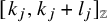 $[k_j,k_j+l_j]_{{\scriptscriptstyle \mathbb {Z}}}$
,
$[k_j,k_j+l_j]_{{\scriptscriptstyle \mathbb {Z}}}$
, $j=1,\dots ,s$
, where
$j=1,\dots ,s$
, where $k_{j+1}-k_j-l_j\ge 1$
. Then
$k_{j+1}-k_j-l_j\ge 1$
. Then $l_1+\dots +l_s=n-t$
. We form the set
$l_1+\dots +l_s=n-t$
. We form the set $\Omega $
as follows:
$\Omega $
as follows: $\Omega $
consists of all t zeros of the first type and
$\Omega $
consists of all t zeros of the first type and $n+1-t$
points from the closed segments
$n+1-t$
points from the closed segments $\Omega _j$
,
$\Omega _j$
, $j=1,\dots ,s$
, of sign changes. In more detail, set
$j=1,\dots ,s$
, of sign changes. In more detail, set $\Omega _1=[k_1,k_1+l_1]_{{\scriptscriptstyle \mathbb {Z}}}$
and construct
$\Omega _1=[k_1,k_1+l_1]_{{\scriptscriptstyle \mathbb {Z}}}$
and construct $\Omega _j$
,
$\Omega _j$
, $j=2,\dots ,s$
, such that either
$j=2,\dots ,s$
, such that either $\Omega _j=[k_j,k_j+l_j-1]_{{\scriptscriptstyle \mathbb {Z}}}$
or
$\Omega _j=[k_j,k_j+l_j-1]_{{\scriptscriptstyle \mathbb {Z}}}$
or $\Omega _j=[k_j+1 ,k_j+l_j]_{{\scriptscriptstyle \mathbb {Z}}}$
. Note that the number of points in closed segments is equal to
$\Omega _j=[k_j+1 ,k_j+l_j]_{{\scriptscriptstyle \mathbb {Z}}}$
. Note that the number of points in closed segments is equal to $(l_1+1)+l_2+\dots +l_s=n+1-t$
.
$(l_1+1)+l_2+\dots +l_s=n+1-t$
.
If $r_1+i$
,
$r_1+i$
, $i=0,\dots ,l_1$
, are the indices of the points
$i=0,\dots ,l_1$
, are the indices of the points $k_1+i$
of the set
$k_1+i$
of the set $\Omega $
in
$\Omega $
in $\Omega _1$
and
$\Omega _1$
and $p(k_1+i)=(-1)^{i_1 +k_1+i}|p(k_1+i)|$
, then
$p(k_1+i)=(-1)^{i_1 +k_1+i}|p(k_1+i)|$
, then $k_1+i=\nu _{r_1+i}$
and
$k_1+i=\nu _{r_1+i}$
and
 $$\begin{align*}\sum_{i=0}^{l_1}(-1)^{r_1+i}p(\nu_{r_1+i})=(-1)^{i_1+k_1+r_1}\sum_{i=0}^{l_1}|p(\nu_{r_1+i})|. \end{align*}$$
Let the segments $\Omega _m$
, for
$\Omega _m$
, for $m=1,\dots ,j-1$
, have already been constructed. Let
$m=1,\dots ,j-1$
, have already been constructed. Let $r_j+i$
,
$r_j+i$
, $i=0,\dots ,l_j-1$
, be the indices of points of the set
$i=0,\dots ,l_j-1$
, be the indices of points of the set $\Omega $
in
$\Omega $
in $\Omega _j$
and
$\Omega _j$
and $p(k_j+i)=(-1)^{i_j+k_j+i}|p(k_j+i)|$
,
$p(k_j+i)=(-1)^{i_j+k_j+i}|p(k_j+i)|$
, $i=0,\dots ,l_j$
.
$i=0,\dots ,l_j$
.
If $(-1)^{i_j+k_j+r_j}=(-1)^{i_1+k_1+r_1}$
, then we set
$(-1)^{i_j+k_j+r_j}=(-1)^{i_1+k_1+r_1}$
, then we set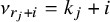 $\nu _{r_j+i}=k_j+i$
,
$\nu _{r_j+i}=k_j+i$
, $i=0, \dots ,l_j-1$
. We have
$i=0, \dots ,l_j-1$
. We have
 $$\begin{align*}\sum_{i=0}^{l_j-1}(-1)^{r_j+i}p(\nu_{r_j+i})=\sum_{i=0}^{l_j-1}(-1)^{r_j+i}p(k_j+i)=(-1)^{i_1+k_1+r_1}\sum_{i=0}^{l_j-1}|p(\nu_{r_j+i})|. \end{align*}$$
If $(-1)^{i_j+k_j+r_j+1}=(-1)^{i_1+k_1+r_1}$
, then we put
$(-1)^{i_j+k_j+r_j+1}=(-1)^{i_1+k_1+r_1}$
, then we put $\nu _{r_j+i}=k_j+i+1$
,
$\nu _{r_j+i}=k_j+i+1$
, $ i=0,\dots ,l_j-1$
. Again, we have
$ i=0,\dots ,l_j-1$
. Again, we have
 $$\begin{align*}\sum_{i=0}^{l_j-1}(-1)^{r_j+i}p(\nu_{r_j+i})=\sum_{i=0}^{l_j-1}(-1)^{r_j+i}p(k_j+i+1)=(-1)^{i_1+k_1+r_1}\sum_{i=0}^{l_j-1}|p(\nu_{r_j+i})|. \end{align*}$$
Thus, the set $\Omega =\{0\le \nu _1<\dots <\nu _{n+1}\le q\}$
is constructed. For this set, in view of (2.4), there holds
$\Omega =\{0\le \nu _1<\dots <\nu _{n+1}\le q\}$
is constructed. For this set, in view of (2.4), there holds
 $$ \begin{align*} 0&=\sum_{i=1}^{n+1}(-1)^{i}p(\nu_i)=\sum_{i=0}^{l_1}(-1)^{r_1+i}p(\nu_{r_1+i})+\sum_{j=2}^s\sum_{i=0}^{l_j-1}(-1)^{r_j+i}p(\nu_{r_j+i})\\& =(-1)^{i_1+k_1+r_1}\Big\{\sum_{i=0}^{l_1}|p(\nu_{r_1+i})|+\sum_{j=2}^s\sum_{i=0}^{l_j-1}|p(\nu_{r_j+i})|\Big\}. \end{align*} $$
Hence, $p(\nu _i)=0$
for
$p(\nu _i)=0$
for $i=1,\dots ,n+1$
. Then we deduce that
$i=1,\dots ,n+1$
. Then we deduce that $p\equiv 0$
, completing the proof.
$p\equiv 0$
, completing the proof.
Proof of Theorem 1.4
By Lemma 2.3, (a) implies (b) and by Lemma 2.4, items (b) and (c) are equivalent. Finally, applying Lemmas 2.2 and 2.5, (a) follows from (b). The proof is now complete.
Proof of Corollary 1.6
To prove this result, it is sufficient to show the following analogue of Lemma 2.5:
If $S^{+}(p)=n$
, then there exists a set
$S^{+}(p)=n$
, then there exists a set $\Omega =\{0\le \nu _1<\dots <\nu _{n+1}\le q\}$
such that if for some positive numbers
$\Omega =\{0\le \nu _1<\dots <\nu _{n+1}\le q\}$
such that if for some positive numbers $\{\rho _i\}_{i=1}^{n+1}$
property (2.4) holds, then
$\{\rho _i\}_{i=1}^{n+1}$
property (2.4) holds, then $p\equiv 0$
.
$p\equiv 0$
.
The construction of the set $\Omega $
is similar to the one in Lemma 2.5, so we will only sketch the proof. As above, we assume that each
$\Omega $
is similar to the one in Lemma 2.5, so we will only sketch the proof. As above, we assume that each $\rho _i=1$
.
$\rho _i=1$
.
Let us consider four different types of intervals. An interval of the first type is a closed segment of sign changes (see the proof of Lemma 2.5). An interval of the second type is $I=[k,k+l]_{{\scriptscriptstyle \mathbb {Z}}}$
, for which
$I=[k,k+l]_{{\scriptscriptstyle \mathbb {Z}}}$
, for which
 $$\begin{align*}p(k)p(k+l)>0,\quad p(k+1)=\dots=p(k+l-1)=0\quad \text{and}\quad l-1 \text{ is odd}. \end{align*}$$
An interval of the third type is $I=[k,k+l]_{{\scriptscriptstyle \mathbb {Z}}}$
, for which
$I=[k,k+l]_{{\scriptscriptstyle \mathbb {Z}}}$
, for which
 $$\begin{align*}p(k)p(k+l)<0,\quad p(k+1)=\dots=p(k+l-1)=0\quad \text{and}\quad l-1 \text{ is even}. \end{align*}$$
It is worth mentioning that intervals of the second and third types contribute to an increase in the number of zeros of the polynomial when zero values are changed to nonzero values, as $N(p,[k,k+l]_{{\scriptscriptstyle \mathbb {Z}}})=l-1$
and
$N(p,[k,k+l]_{{\scriptscriptstyle \mathbb {Z}}})=l-1$
and $S^{+}(p,[k,k+l]_{{\scriptscriptstyle \mathbb {Z}}})=l$
.
$S^{+}(p,[k,k+l]_{{\scriptscriptstyle \mathbb {Z}}})=l$
.
Intervals of the fourth type are $I=[k,k+l]_{{\scriptscriptstyle \mathbb {Z}}}$
, consisting of zeros of the first type, for which one of the following conditions holds: (i)
$I=[k,k+l]_{{\scriptscriptstyle \mathbb {Z}}}$
, consisting of zeros of the first type, for which one of the following conditions holds: (i) $k=0$
, (ii)
$k=0$
, (ii) $k+l=q$
, (iii)
$k+l=q$
, (iii) $l+1$
is odd and
$l+1$
is odd and $p(k-1)p(k+l+1)<0$
, (iv)
$p(k-1)p(k+l+1)<0$
, (iv) $l+1$
is even and
$l+1$
is even and $p(k-1)p(k +l+1)>0$
. Note that changing zero values of p to any nonzero numbers at points of intervals of the fourth type cannot increase the number of its zeros.
$p(k-1)p(k +l+1)>0$
. Note that changing zero values of p to any nonzero numbers at points of intervals of the fourth type cannot increase the number of its zeros.
Denote the sets of intervals of the first, second, third, and fourth types by $\Sigma _1$
,
$\Sigma _1$
, $\Sigma _2$
,
$\Sigma _2$
, $\Sigma _3$
, and
$\Sigma _3$
, and $\Sigma _4$
, respectively. Set
$\Sigma _4$
, respectively. Set $\Sigma =\cup _{i=1}^{3}\Sigma _i$
. Note that intervals from different sets
$\Sigma =\cup _{i=1}^{3}\Sigma _i$
. Note that intervals from different sets $\Sigma _i$
can intersect only at their endpoints.
$\Sigma _i$
can intersect only at their endpoints.
We have
 $$\begin{align*}n=\sum_{I\in\Sigma_1}(|I|-1)+\sum_{I\in\Sigma_2}(|I|-1)+\sum_{I\in\Sigma_3}(|I|-1)+\sum_{I\in\Sigma_4}|I|. \end{align*}$$
By $\Omega $
we define a set of allFootnote
5
points of the intervals from
$\Omega $
we define a set of allFootnote
5
points of the intervals from $\Sigma $
and
$\Sigma $
and $\Sigma _4$
. Then the cardinality of
$\Sigma _4$
. Then the cardinality of $\Omega $
is
$\Omega $
is
 $$\begin{align*}1+\sum_{I\in\Sigma_1}(|I|-1)+\sum_{I\in\Sigma_2}(|I|-1)+\sum_{I\in\Sigma_3}(|I|-1)+\sum_{I\in\Sigma_4}|I|=n+1. \end{align*}$$
Let now $[\nu _{r_1},\nu _{r_1}+l_{r_1}]_{{\scriptscriptstyle \mathbb {Z}}}\subset \Omega $
be the first interval from
$[\nu _{r_1},\nu _{r_1}+l_{r_1}]_{{\scriptscriptstyle \mathbb {Z}}}\subset \Omega $
be the first interval from $\Sigma $
and, for some integer
$\Sigma $
and, for some integer $i_0$
,
$i_0$
, $(-1)^{i_0+r_1}p(\nu _{r_1})>0$
. Note that, for
$(-1)^{i_0+r_1}p(\nu _{r_1})>0$
. Note that, for $r_1\ge 2$
,
$r_1\ge 2$
, $0\le \nu _1<\dots <\nu _{r_1-1}$
are the points of the set
$0\le \nu _1<\dots <\nu _{r_1-1}$
are the points of the set $\Omega \cap \Sigma _4.$
Then
$\Omega \cap \Sigma _4.$
Then $(-1)^{i_0+r_1+i}p(\nu _{r_1}+i)\ge 0$
,
$(-1)^{i_0+r_1+i}p(\nu _{r_1}+i)\ge 0$
, $i=0,\dots ,l_{r_1}$
.
$i=0,\dots ,l_{r_1}$
.
Proceeding similarly, let $0\le \nu _1<\dots <\nu _{r_2-1}$
be the points of the set
$0\le \nu _1<\dots <\nu _{r_2-1}$
be the points of the set $\Omega $
that have been constructed, and the second interval
$\Omega $
that have been constructed, and the second interval $I=[k,k+l]_{{\scriptscriptstyle \mathbb {Z}}}\in \Sigma $
is such that
$I=[k,k+l]_{{\scriptscriptstyle \mathbb {Z}}}\in \Sigma $
is such that $k=\nu _{r_2}$
or
$k=\nu _{r_2}$
or $k=\nu _{r_2}-1$
. If
$k=\nu _{r_2}-1$
. If $(-1)^{i_0+r_2}p(k)>0$
, then we include in
$(-1)^{i_0+r_2}p(k)>0$
, then we include in $\Omega $
the points of the interval
$\Omega $
the points of the interval $[\nu _{r_2},\nu _{r_2}+l_{r_2}]_{{\scriptscriptstyle \mathbb {Z}}}$
, where
$[\nu _{r_2},\nu _{r_2}+l_{r_2}]_{{\scriptscriptstyle \mathbb {Z}}}$
, where $\nu _{r_2}=k$
and
$\nu _{r_2}=k$
and $l_{r_2}=l-1$
. Otherwise, we include in
$l_{r_2}=l-1$
. Otherwise, we include in $\Omega $
the points of the interval
$\Omega $
the points of the interval $[\nu _{r_2},\nu _{r_2}+l_{r_2}]_{{\scriptscriptstyle \mathbb {Z}}}$
, where
$[\nu _{r_2},\nu _{r_2}+l_{r_2}]_{{\scriptscriptstyle \mathbb {Z}}}$
, where $\nu _{r_2}=k+1$
and
$\nu _{r_2}=k+1$
and $l_{r_2}=l$
. In both cases,
$l_{r_2}=l$
. In both cases, $|[\nu _{r_2},\nu _{r_2}+l_{r_2}]_{{\scriptscriptstyle \mathbb {Z}}}|=|I|-1$
and
$|[\nu _{r_2},\nu _{r_2}+l_{r_2}]_{{\scriptscriptstyle \mathbb {Z}}}|=|I|-1$
and $(-1)^{i_0+r_2+i}p(\nu _{r_2}+i)\ge 0$
,
$(-1)^{i_0+r_2+i}p(\nu _{r_2}+i)\ge 0$
, $i=0,\dots ,l_{r_2}$
.
$i=0,\dots ,l_{r_2}$
.
Continuing in the same way, we complete the construction of the set $\Omega $
. Then, according to (2.4),
$\Omega $
. Then, according to (2.4),
 $$\begin{align*}0=\sum_{i=1}^{n+1}(-1)^{i}p(\nu_i)=(-1)^{i_0}\sum_{i=1}^{n+1}|p(\nu_i)|. \end{align*}$$
From this, $p(\nu _i)=0$
for
$p(\nu _i)=0$
for $i=1,\dots ,n+1$
. Therefore,
$i=1,\dots ,n+1$
. Therefore, $p\equiv 0$
, completing the proof.
$p\equiv 0$
, completing the proof.
The proof of Corollary 1.6 immediately implies the following result.
Corollary 2.6. If the set $\{\varphi _k\}_{k=1}^n\subset C[0,q]_{{\scriptscriptstyle \mathbb {Z}}}$
is a
$\{\varphi _k\}_{k=1}^n\subset C[0,q]_{{\scriptscriptstyle \mathbb {Z}}}$
is a $T_{{\scriptscriptstyle \mathbb {Z}}}$
-system,
$T_{{\scriptscriptstyle \mathbb {Z}}}$
-system, $p\in L_n$
, and
$p\in L_n$
, and $N(p)=n-1$
, then the polynomial p has no intervals of the second and third types.
$N(p)=n-1$
, then the polynomial p has no intervals of the second and third types.
To conclude this section, we give an example of a $T_0$
-system which is not a
$T_0$
-system which is not a $T_{{\scriptscriptstyle \mathbb {Z}}}$
-system.
$T_{{\scriptscriptstyle \mathbb {Z}}}$
-system.
Example 2.7. For $k=1,\dots ,q-1$
, define
$k=1,\dots ,q-1$
, define
 $$\begin{align*}\varphi_k(\nu)= \begin{cases} 0,&\nu=0,\dots,k-2,k,\dots,q-1,\\ 1,&\nu=k-1,q, \end{cases} \quad\varphi_q(\nu)= \begin{cases} 0,&\nu=0,\dots,q-2,\\ 1,&\nu=q-1,\\ -1,&\nu=q. \end{cases} \end{align*}$$
Then $\dim {L_q}=q$
and
$\dim {L_q}=q$
and $N_0(\varphi _k)=q-1$
,
$N_0(\varphi _k)=q-1$
, $k=1,\dots ,q$
. Note that the function
$k=1,\dots ,q$
. Note that the function $\varphi _q(\nu )$
has a zero of the second type at the point q and hence
$\varphi _q(\nu )$
has a zero of the second type at the point q and hence $N(\varphi _q)=q$
.
$N(\varphi _q)=q$
.
For an arbitrary polynomial $p(\nu )=\sum _{k=1}^qa_k\varphi _k(\nu )$
, the following equalities hold:
$p(\nu )=\sum _{k=1}^qa_k\varphi _k(\nu )$
, the following equalities hold:
 $$ \begin{align} p(\nu)= \begin{cases} a_{\nu+1},&\nu=0,\dots,q-1,\\ a_1+\dots+a_{q-1}-a_q,&\nu=q. \end{cases} \end{align} $$
If p has q zeros of the first type, then either all coefficients of the polynomial are zero, or $q-1$
coefficients are zero and
$q-1$
coefficients are zero and $a_1+\dots +a_{q-1}-a_q=0$
, that is, in any case all coefficients of p are zeros. Therefore, if p is nontrivial,
$a_1+\dots +a_{q-1}-a_q=0$
, that is, in any case all coefficients of p are zeros. Therefore, if p is nontrivial, $N_0(p)\le q-1$
. Thus, the set
$N_0(p)\le q-1$
. Thus, the set $\{\varphi _k\}_{k=1}^q$
is a
$\{\varphi _k\}_{k=1}^q$
is a $T_0$
-system but not a
$T_0$
-system but not a $T_{{\scriptscriptstyle \mathbb {Z}}}$
-system.
$T_{{\scriptscriptstyle \mathbb {Z}}}$
-system.
Further, define for any $f\in C[0,q]_{{\scriptscriptstyle \mathbb {Z}}}$
 $$\begin{align*}p^{*}(\nu)=\sum_{k=1}^{q-1}(f(k-1)+\delta)\varphi_k(\nu)+(f(q-1)-\delta)\varphi_q(\nu), \end{align*}$$
where
 $$\begin{align*}\delta=-\frac{1}{q+1}\Big(\,\sum_{k=1}^{q-1}f(k-1)-f(q-1)-f(q)\Big). \end{align*}$$
By (2.5), we have
 $$\begin{align*}p^{*}(\nu)= \begin{cases} f(\nu)+\delta,&\nu=0,\dots,q-2,\\ f(\nu)-\delta,&\nu=q-1,q. \end{cases} \end{align*}$$
If $\delta =0$
, then
$\delta =0$
, then $f\equiv p^{*}\in L_q$
and
$f\equiv p^{*}\in L_q$
and $E_q(f,L_q)_{\infty }=0$
. If
$E_q(f,L_q)_{\infty }=0$
. If $\delta \neq 0$
,
$\delta \neq 0$
, $e(\nu )=p^{*}(\nu )-f(\nu )$
,
$e(\nu )=p^{*}(\nu )-f(\nu )$
,
 $$\begin{align*}\varepsilon_{\nu}= \begin{cases} \operatorname{sign} \delta,&\nu=0,\dots,q-2,\\ -\operatorname{sign} \delta,&\nu=q-1,q, \end{cases} \end{align*}$$
then, by Theorem 1.3, for $\nu \in [0,q]_{{\scriptscriptstyle \mathbb {Z}}}$
and all polynomials
$\nu \in [0,q]_{{\scriptscriptstyle \mathbb {Z}}}$
and all polynomials $p\in L_q$
 $$\begin{align*}\varepsilon_{\nu} e(\nu)=\|e\|_{\infty}=|\delta|,\qquad \sum_{\nu=0}^{q}\varepsilon_{\nu} p(\nu)=0. \end{align*}$$
Consequently, $p^{*}\in L_q$
is the unique best uniform approximant of the function f and
$p^{*}\in L_q$
is the unique best uniform approximant of the function f and $E_q(f,L_q)_{\infty }=|\delta |$
. Note that the metric projection operator
$E_q(f,L_q)_{\infty }=|\delta |$
. Note that the metric projection operator $Pf=p^{*}$
onto the q-dimensional subspace
$Pf=p^{*}$
onto the q-dimensional subspace $L_q$
is linear (see, e.g., [Reference Borodin6]), and for any function
$L_q$
is linear (see, e.g., [Reference Borodin6]), and for any function $f\not \in L_q$
, the polynomial
$f\not \in L_q$
, the polynomial $Pf$
does not admit a Chebyshev alternance set of length
$Pf$
does not admit a Chebyshev alternance set of length $q+1$
.
$q+1$
.
3 Proofs of Theorems 1.8, 1.10, and 1.11
Proof of Theorem 1.8
Let $k_{l}>0$
be the leading coefficient of the polynomial
$k_{l}>0$
be the leading coefficient of the polynomial $P_{l}(\lambda )$
. Then, by (1.7), we have
$P_{l}(\lambda )$
. Then, by (1.7), we have $\beta _{l}k_{l+1}=\rho _{l}k_{l}$
. Using this, for the monic polynomials
$\beta _{l}k_{l+1}=\rho _{l}k_{l}$
. Using this, for the monic polynomials $Q_{l}(\lambda )=k_{l}^{-1}P_{l}(\lambda )$
, we obtain the recurrence relation
$Q_{l}(\lambda )=k_{l}^{-1}P_{l}(\lambda )$
, we obtain the recurrence relation
 $$\begin{align*}B_{l}Q_{l-1}(\lambda)+A_{l}Q_{l}(\lambda)+Q_{l+1}(\lambda)=\lambda Q_{l}(\lambda), \end{align*}$$
where $B_{0}>0$
is arbitrary and
$B_{0}>0$
is arbitrary and
 $$ \begin{align} A_{l}=\frac{\alpha_{l}}{\rho_{l}},\quad B_{l}=\frac{\gamma_{l-1}\beta_{l-1}}{\rho_{l-1}\rho_{l}}= \frac{\gamma_{l-1}\rho_{l-1}k_{l-1}^{2}}{\beta_{l-1}\rho_{l}k_{l}^{2}}. \end{align} $$
We have $A_{l}\in \mathbb {R}$
and
$A_{l}\in \mathbb {R}$
and $B_{l}>0$
for any
$B_{l}>0$
for any $l\ge 0$
. These conditions are necessary and sufficient in Favard’s theorem [Reference Chihara8, Ch. II, Th. 6.4] on the existence of a nondecreasing function of bounded variation with infinite spectrum which generates a positive measure
$l\ge 0$
. These conditions are necessary and sufficient in Favard’s theorem [Reference Chihara8, Ch. II, Th. 6.4] on the existence of a nondecreasing function of bounded variation with infinite spectrum which generates a positive measure $\mu $
such that
$\mu $
such that
 $$\begin{align*}\int_{\mathbb{R}}Q_{l}(\lambda)Q_{m}(\lambda)\,d\mu(\lambda)=B_{0}B_{1}\cdots B_{l}\delta_{lm}. \end{align*}$$
Now, to show (1.8), it is enough to set $B_{0}=\rho _{0}^{-1}$
.
$B_{0}=\rho _{0}^{-1}$
.
According to [Reference Chihara8, Ch. IV, Th. 2.2], the measure $\mu $
has a finite support
$\mu $
has a finite support $[a,b]$
if and only if the sequences
$[a,b]$
if and only if the sequences $A_{l}$
and
$A_{l}$
and $B_{l}$
are uniformly bounded. In this case, the endpoints of the interval
$B_{l}$
are uniformly bounded. In this case, the endpoints of the interval $[a,b]$
will be the limit points of the zeros of
$[a,b]$
will be the limit points of the zeros of $Q_{l}(\lambda )$
, and, therefore, of
$Q_{l}(\lambda )$
, and, therefore, of $P_{l}(\lambda )$
as well. By (3.1), the boundedness of
$P_{l}(\lambda )$
as well. By (3.1), the boundedness of $A_{l}$
and
$A_{l}$
and $B_{l}$
is equivalent to the boundedness of the sequences (1.9), which completes the proof.
$B_{l}$
is equivalent to the boundedness of the sequences (1.9), which completes the proof.
Proof of Theorem 1.10
Recall that $\lambda _{l,l}<\dots <\lambda _{1,l}$
are the zeros of the polynomials
$\lambda _{l,l}<\dots <\lambda _{1,l}$
are the zeros of the polynomials $P_l(\lambda )$
,
$P_l(\lambda )$
, $l\in \mathbb {N}$
, and
$l\in \mathbb {N}$
, and $\lambda _{q+1}<\dots <\lambda _{1}$
are zeros of the polynomial
$\lambda _{q+1}<\dots <\lambda _{1}$
are zeros of the polynomial $\widetilde {P}_{q+1}(\lambda )$
, cf. (1.10).
$\widetilde {P}_{q+1}(\lambda )$
, cf. (1.10).
In what follows, we will use the fact that the zeros of orthogonal polynomials $P_{l-1}(\lambda )$
and
$P_{l-1}(\lambda )$
and $P_l(\lambda )$
,
$P_l(\lambda )$
, $l\in [2,q]_{{\scriptscriptstyle \mathbb {Z}}}$
, as well as
$l\in [2,q]_{{\scriptscriptstyle \mathbb {Z}}}$
, as well as $P_q(\lambda )$
and
$P_q(\lambda )$
and $\widetilde {P}_{q+1}(\lambda )$
, interlace (see [Reference Szegö35, Ch. III, § 3.3]):
$\widetilde {P}_{q+1}(\lambda )$
, interlace (see [Reference Szegö35, Ch. III, § 3.3]):
 $$ \begin{align} \begin{gathered} \lambda_{l,l}<\lambda_{l-1,l-1}<\lambda_{l-1,l}<\lambda_{l-2,l-1}<\dots< \lambda_{2,l-1}<\lambda_{2,l}<\lambda_{1,l-1}<\lambda_{1,l},\\ \lambda_{q+1}<\lambda_{q,q}<\lambda_{q}<\lambda_{q-1,q}<\dots< \lambda_{2,q}<\lambda_{2}<\lambda_{1,q}<\lambda_{1}. \end{gathered} \end{align} $$
Let the interval $(a,b)$
contain the zeros of the polynomial
$(a,b)$
contain the zeros of the polynomial $P_q(\lambda )$
and let
$P_q(\lambda )$
and let $k\in [1,q+1]_{{\scriptscriptstyle \mathbb {Z}}}$
. If
$k\in [1,q+1]_{{\scriptscriptstyle \mathbb {Z}}}$
. If $s=0$
, then
$s=0$
, then $\psi _{k}(0)=P_0(\lambda _{k})=1$
, so further
$\psi _{k}(0)=P_0(\lambda _{k})=1$
, so further $s\in [1,q]_{{\scriptscriptstyle \mathbb {Z}}}$
.
$s\in [1,q]_{{\scriptscriptstyle \mathbb {Z}}}$
.
We will also use the following observation. If $s\in [1,q]_{{\scriptscriptstyle \mathbb {Z}}}$
,
$s\in [1,q]_{{\scriptscriptstyle \mathbb {Z}}}$
, $l\in [1,s]_{{\scriptscriptstyle \mathbb {Z}}}$
,
$l\in [1,s]_{{\scriptscriptstyle \mathbb {Z}}}$
, $\lambda _{s+1,s}=a$
,
$\lambda _{s+1,s}=a$
, $\lambda _ {0,s}=b$
, and
$\lambda _ {0,s}=b$
, and $\lambda _{l,s}<\lambda _{k}<\lambda _{l-1,s}$
, then
$\lambda _{l,s}<\lambda _{k}<\lambda _{l-1,s}$
, then
 $$ \begin{align} \operatorname{sign} \psi_k(s)=\operatorname{sign} P_s(\lambda_{k})=(-1)^{l-1}, \end{align} $$
and if $\lambda _{k}=\lambda _{l,s}$
or
$\lambda _{k}=\lambda _{l,s}$
or $\lambda _{k}=\lambda _{l-1,s}$
, then
$\lambda _{k}=\lambda _{l-1,s}$
, then
 $$ \begin{align} \psi_k(s)=P_s(\lambda_{k})=P_s(\lambda_{l,s})=P_s(\lambda_{l-1,s})=0. \end{align} $$
Further, for $k=1$
and
$k=1$
and $s\in [1,q]_{{\scriptscriptstyle \mathbb {Z}}}$
, the inequality
$s\in [1,q]_{{\scriptscriptstyle \mathbb {Z}}}$
, the inequality $\lambda _{1,s}<\lambda _{1}$
yields
$\lambda _{1,s}<\lambda _{1}$
yields
 $$ \begin{align} \psi_1(s)>0,\quad s\in [0,q]_{{\scriptscriptstyle\mathbb{Z}}}. \end{align} $$
Therefore, $N(\psi _1)=0$
. For
$N(\psi _1)=0$
. For $k=q+1$
and
$k=q+1$
and $s\in [1,q]_{{\scriptscriptstyle \mathbb {Z}}}$
, from the inequalities (3.2) we have
$s\in [1,q]_{{\scriptscriptstyle \mathbb {Z}}}$
, from the inequalities (3.2) we have $\lambda _{q+1}<\lambda _{s,s}$
, so
$\lambda _{q+1}<\lambda _{s,s}$
, so $\operatorname {sign} \psi _{q+1}(s)=(-1)^{s}$
and
$\operatorname {sign} \psi _{q+1}(s)=(-1)^{s}$
and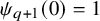 $\psi _{q+1}(0)=1$
. Thus,
$\psi _{q+1}(0)=1$
. Thus, $N(\psi _{q+1})=q$
.
$N(\psi _{q+1})=q$
.
Let $k\in [2,q]_{{\scriptscriptstyle \mathbb {Z}}}$
. Since, according to (3.2),
$k\in [2,q]_{{\scriptscriptstyle \mathbb {Z}}}$
. Since, according to (3.2),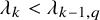 $\lambda _{k}<\lambda _{k-1,q}$
, there exists a smallest
$\lambda _{k}<\lambda _{k-1,q}$
, there exists a smallest $i_1\le q$
for which
$i_1\le q$
for which
 $$ \begin{align} \lambda_{k,i_1}<\lambda_{k-1,i_1-1}\le\lambda_{k}<\lambda_{k-1,i_1},\quad i_1\ge k. \end{align} $$
If $i_1\le s\le q$
, then, by (3.2) and (3.6),
$i_1\le s\le q$
, then, by (3.2) and (3.6),
 $$\begin{align*}\lambda_{k,i_1}\le\lambda_{k,s}\le \lambda_{k,q}< \lambda_{k}<\lambda_{k-1,i_1}\le\lambda_{k-1,s}\le\lambda_{k-1,q}. \end{align*}$$
Using (3.3), we then derive
 $$ \begin{align} \operatorname{sign} \psi_k(s)=(-1)^{k-1}. \end{align} $$
Since, according to (3.2), $\lambda _{k}<\lambda _{k-1,i_1}<\lambda _{k-2,i_1-1}$
, there exists a smallest
$\lambda _{k}<\lambda _{k-1,i_1}<\lambda _{k-2,i_1-1}$
, there exists a smallest $i_2\le i_1-1 $
for which
$i_2\le i_1-1 $
for which
 $$ \begin{align} \lambda_{k-1,i_2}<\lambda_{k-2,i_2-1}\le\lambda_{k}<\lambda_{k-2,i_2}, \quad i_2\ge k-1. \end{align} $$
If $i_2\le s<i_1-1$
, then, by (3.2), (3.6) and (3.8),
$i_2\le s<i_1-1$
, then, by (3.2), (3.6) and (3.8),
 $$\begin{align*}\lambda_{k-1,i_2}\le\lambda_{k-1,s}<\lambda_{k-1,i_1-1}\le\lambda_{k}<\lambda_{k-2,i_2}\le\lambda_{k-2,s}<\lambda_{k-2,i_1-1}. \end{align*}$$
Therefore, using (3.3) and (3.4), we obtain
 $$\begin{align*}\operatorname{sign} \psi_k(s)=(-1)^{k-2},\quad \operatorname{sign} \psi_k(i_1-1)=(-1)^{k-2}\vee 0. \end{align*}$$
Proceeding similarly for $j\in [2,k-1]_{{\scriptscriptstyle \mathbb {Z}}}$
, we construct points
$j\in [2,k-1]_{{\scriptscriptstyle \mathbb {Z}}}$
, we construct points $\{i_j\}_{j=1}^{k-1}$
such that
$\{i_j\}_{j=1}^{k-1}$
such that
 $$\begin{align*}k-j+1\le i_j\le i_{j-1}-1, \quad \lambda_{k-j+1,i_j}<\lambda_{k-j,i_j-1}\le\lambda_{k}<\lambda_{k-j,i_j}, \end{align*}$$
and for $i_j\le s<i_{j-1}-1$
 $$\begin{align*}\lambda_{k+1-j,i_j}\le\lambda_{k+1-j,s}<\lambda_{k+1-j,i_{j-1}-1}\le\lambda_{k}<\lambda_{k-j,i_j}\le\lambda_{k-j,s}<\lambda_{k-j,i_{j-1}-1}, \end{align*}$$
 $$ \begin{align} \operatorname{sign} \psi_k(s)=(-1)^{k-j},\quad \operatorname{sign} \psi_k(i_{j-1}-1)=(-1)^{k-j}\vee 0. \end{align} $$
In the case $1\le s<i_{k-1}-1$
, we have
$1\le s<i_{k-1}-1$
, we have $\lambda _{1,s}<\lambda _{1,i_{k-1}-1}\le \lambda _{k}$
. Hence, in light of (3.2),
$\lambda _{1,s}<\lambda _{1,i_{k-1}-1}\le \lambda _{k}$
. Hence, in light of (3.2),
 $$ \begin{align} \operatorname{sign} \psi_k(s)=1,\quad \operatorname{sign} \psi_k(i_{k-1}-1)=1\vee 0. \end{align} $$
If for all $j\in [2, k-1]_{{\scriptscriptstyle \mathbb {Z}}}$
,
$j\in [2, k-1]_{{\scriptscriptstyle \mathbb {Z}}}$
, $\lambda _{k-j,i_j-1}\neq \lambda _{k}$
, then, according to (3.7), (3.9), (3.10), only the points
$\lambda _{k-j,i_j-1}\neq \lambda _{k}$
, then, according to (3.7), (3.9), (3.10), only the points $\nu _j=i_j$
,
$\nu _j=i_j$
, $j\in [1,k-1]_{{\scriptscriptstyle \mathbb {Z}}}$
, are zeros of
$j\in [1,k-1]_{{\scriptscriptstyle \mathbb {Z}}}$
, are zeros of $\psi _k(\nu )$
and, moreover,
$\psi _k(\nu )$
and, moreover, $N(\psi _k)=k-1$
.
$N(\psi _k)=k-1$
.
Let $\psi _k(i_j-1)=0$
. Since
$\psi _k(i_j-1)=0$
. Since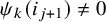 $\psi _k(i_{j+1})\neq 0$
, it follows that
$\psi _k(i_{j+1})\neq 0$
, it follows that $i_{j+1}\le i_j-2<i_j-1$
and
$i_{j+1}\le i_j-2<i_j-1$
and
 $$\begin{align*}\operatorname{sign}{}(\psi_k(i_{j}-2)\psi_k(i_{j}))=(-1)^{k-j-1}(-1)^{k-j}=-1. \end{align*}$$
Therefore, the zero $\nu _j=i_j$
is replaced by
$\nu _j=i_j$
is replaced by $\nu _j=i_j-1$
and we again have
$\nu _j=i_j-1$
and we again have $N(\psi _k)=k-1$
. Along the way, we proved that if
$N(\psi _k)=k-1$
. Along the way, we proved that if $\psi _{k}(\nu )=0$
,
$\psi _{k}(\nu )=0$
, $k\in [2,q]_{{\scriptscriptstyle \mathbb {Z}}}$
, then
$k\in [2,q]_{{\scriptscriptstyle \mathbb {Z}}}$
, then $\nu \in [1,q-1]_ {{\scriptscriptstyle \mathbb {Z}}}$
and
$\nu \in [1,q-1]_ {{\scriptscriptstyle \mathbb {Z}}}$
and $\psi _{k}(\nu -1)\psi _{k}(\nu +1)<0$
. This implies that
$\psi _{k}(\nu -1)\psi _{k}(\nu +1)<0$
. This implies that $S^{-}(\psi _k)=S^{+}(\psi _k)=k-1$
, completing the proof.
$S^{-}(\psi _k)=S^{+}(\psi _k)=k-1$
, completing the proof.
3.1 Proof of Theorem 1.11
Step 1. First, let us rewrite the discrete Sturm-Liouville problems (1.7) and (1.12) and then derive the Christoffel-Darboux formulas.
The self-adjoint form of the problem (1.7) is given by
 $$ \begin{align*} \nabla(w_l\Delta P_l(\lambda))+c_lP_l(\lambda)=\lambda d_lP_l(\lambda), \quad l\in \mathbb{Z}_{+},\quad \lambda\in\mathbb{C}, \end{align*} $$
where $\Delta b_{l}=b_{l+1}-b_{l}$
,
$\Delta b_{l}=b_{l+1}-b_{l}$
, $\nabla b_{l}=b_{l}-b_{l-1}$
are the forward and backward differences, respectively,
$\nabla b_{l}=b_{l}-b_{l-1}$
are the forward and backward differences, respectively, $d_l$
is defined in (1.8), and
$d_l$
is defined in (1.8), and
 $$ \begin{align} w_l=\frac{\beta_ld_l}{\rho_l},\quad c_l=\frac{(\alpha_l+\beta_l+\gamma_{l-1})d_l}{\rho_l}. \end{align} $$
Indeed, using (1.7), (1.8) and (3.11), we obtain
 $$\begin{align*}w_{l-1}=\frac{\gamma_{l-1}d_l}{\rho_l},\quad \nabla(w_l\Delta P_l(\lambda))=w_lP_{l+1}(\lambda)+w_{l-1}P_{l-1}(\lambda)-(w_{l}+w_{l-1})P_{l}(\lambda), \end{align*}$$
and
 $$\begin{align*}\nabla(w_l\Delta P_l(\lambda))+c_lP_l(\lambda)-\lambda d_lP_l(\lambda) =\frac{d_l}{\rho_l}\,\bigl\{\beta_lP_{l+1}(\lambda)+\alpha_lP_{l}(\lambda)+\gamma_{l-1}P_{l-1}(\lambda)-\lambda\rho_lP_{l}(\lambda)\bigr\}. \end{align*}$$
Now we can easily derive the Christoffel-Darboux formula
 $$ \begin{align} \sum_{s=0}^{l}d_{s}P_{s}(x)P_{s}(y)=w_{l}\,\frac{P_{l+1}(x)P_{l}(y)-P_{l}(x)P_{l+1}(y)}{x-y},\quad x\neq y. \end{align} $$
To see this, using the Lagrange formula [Reference Agarwal, Bohner, Grace and O’Regan2]
 $$\begin{align*}(x-y)d_sP_s(x)P_s(y)=P_s(y)\nabla(w_s\Delta P_s(x))-P_s(x)\nabla(w_s\Delta P_s(y)), \end{align*}$$
we have
 $$ \begin{align*}& (x-y)\sum_{s=0}^{l}d_sP_s(x)P_s(y)=\sum_{s=0}^{l}\bigl\{P_s(y)\nabla(w_s\Delta P_s(x))-P_s(x)\nabla(w_s\Delta P_s(y))\bigr\}\\ &=\sum_{s=0}^{l}\bigl\{w_sP_{s+1}(x)P_s(y)+w_{s-1}P_s(y)P_{s-1}(x)-w_sP_{s+1}(y)P_s(x)-w_{s-1}P_{s}(x)P_{s-1}(y)\bigr\}\\ &=w_l\bigl\{P_{l+1}(x)P_l(y)-P_{l}(x)P_{l+1}(y)\bigr\}. \end{align*} $$
Further, by (3.12), it follows that $w_{l}=k_{l}d_{l}/k_{l+1}$
, where
$w_{l}=k_{l}d_{l}/k_{l+1}$
, where $k_{l}$
is the leading coefficient of the polynomial
$k_{l}$
is the leading coefficient of the polynomial $P_{l }$
. Applying (1.8) and (3.11), we get
$P_{l }$
. Applying (1.8) and (3.11), we get
 $$\begin{align*}k_{0}=1,\quad k_{l}=\frac{\rho_0\cdots\rho_{l-1}}{\beta_0\cdots\beta_{l-1}}, \quad l\ge 1. \end{align*}$$
Moreover, the Sturm-Liouville problem (1.12) can also be written in an equivalent self-adjoint form as follows:
 $$ \begin{align} \begin{gathered} \nabla(w_l\Delta \psi(\nu))+c_l\psi(\nu)=\lambda d_l\psi(\nu),\\ \psi(-1)=0,\quad\psi(q+1)-\eta\psi(q)=0. \end{gathered} \end{align} $$
From (3.13), as in the proof of (3.12), we obtain the following Lagrange equality:
 $$ \begin{align*} d_{\nu}(\lambda_l-\lambda_k)\psi_l(\nu)\psi_k(\nu)= \nabla(w_{\nu}\{\psi_l(\nu)\Delta \psi_k(\nu)-\psi_k(\nu)\Delta \psi_l(\nu)\}). \end{align*} $$
It is important to mention that the Christoffel-Darboux formula for the eigenfunctions $\psi _k$
has the form
$\psi _k$
has the form
 $$ \begin{align} \sum_{\nu=0}^{l}d_{\nu}\psi_k(\nu)\psi_s(\nu)=w_{l}\,\frac{\psi_k(l+1)\psi_s(l)-\psi_k(l)\psi_s(l+1)}{\lambda_k-\lambda_s}, \end{align} $$
which immediately implies the discrete orthogonality of the eigenfunctions. Indeed, for $k\neq s$
, due to the boundary condition in (1.12),
$k\neq s$
, due to the boundary condition in (1.12),
 $$ \begin{align*} (\psi_k,\psi_s)&=\sum_{\nu=0}^{q}d_{\nu}\psi_k(\nu)\psi_s(\nu)=w_{q}\,\frac{\psi_k(q+1)\psi_s(q)-\psi_k(q)\psi_s(q+1)}{\lambda_k-\lambda_s}\\ &=w_{q}\,\frac{(\psi_k(q+1)-\eta\psi_k(q))\psi_s(q)-(\psi_s(q+1)-\eta\psi_s(q))\psi_k(q)}{\lambda_k-\lambda_s}=0. \end{align*} $$
Step 2. Now we will prove several lemmas on zeros and sign changes of discrete functions.
Lemma 3.1. If $f\in C[0,q]_{{\scriptscriptstyle \mathbb {Z}}}$
, then
$f\in C[0,q]_{{\scriptscriptstyle \mathbb {Z}}}$
, then
 $$ \begin{align} S^{-}(f)\le N(f)\le S^{+}(f). \end{align} $$
Proof. It suffices to compare $S^{-}(f,[m,n]_{{\scriptscriptstyle \mathbb {Z}}})$
,
$S^{-}(f,[m,n]_{{\scriptscriptstyle \mathbb {Z}}})$
, $N(f,[m,n]_{{\scriptscriptstyle \mathbb {Z}}})$
, and
$N(f,[m,n]_{{\scriptscriptstyle \mathbb {Z}}})$
, and $S ^{+}(f,[m,n]_{{\scriptscriptstyle \mathbb {Z}}})$
at interior points of the intervals
$S ^{+}(f,[m,n]_{{\scriptscriptstyle \mathbb {Z}}})$
at interior points of the intervals $[m,n]_{{\scriptscriptstyle \mathbb {Z}}}$
, where f equals zero. We may assume that
$[m,n]_{{\scriptscriptstyle \mathbb {Z}}}$
, where f equals zero. We may assume that $n-m\ge 2$
.
$n-m\ge 2$
.
-
○ If
$m=0$
,
$f(0)=f(1)=\dots =f(n-1)=0$
, and
$f(n)\neq 0$
, then
$S^{-}(f ,[0,n]_{{\scriptscriptstyle \mathbb {Z}}})=0$
,
$N(f,[0,n]_{{\scriptscriptstyle \mathbb {Z}}})=n$
,
$S^{+}(f,[0,n] _{{\scriptscriptstyle \mathbb {Z}}})=n$
and thus (3.15) is valid. -
○ If
$n=q$
,
$f(m)\neq 0$
,
$f(m+1)=\dots =f(q)=0$
, and
$f(n)\neq 0$
, then
$S^ {-}(f,[m,q]_{{\scriptscriptstyle \mathbb {Z}}})=0$
,
$N(f,[m,q]_{{\scriptscriptstyle \mathbb {Z}}})=q-m$
,
$S^{+}(f, [m,q]_{{\scriptscriptstyle \mathbb {Z}}})=q-m$
and (3.15) follows. -
○ If
$f(m)f(n)<0$
(for example,
$f(m)>0$
,
$f(m+1)=\dots =f(n-1)=0$
,
$f(n )<0$
), then
$S^{-}(f,[m,q]_{{\scriptscriptstyle \mathbb {Z}}})=1$
,
$N(f,[m,q]_{{\scriptscriptstyle \mathbb {Z}}})=n-m-1 $
,
$S^{+}(f,[m,n]_{{\scriptscriptstyle \mathbb {Z}}})=n-m-1$
for even
$n-m$
and
$S^{+}(f,[m,n]_{{\scriptscriptstyle \mathbb {Z}}})=n-m$
for odd
$n-m$
. Hence, (3.15) is valid. -
○ If
$f(m)f(n)>0$
(for example,
$f(m)>0$
,
$f(m+1)=\dots =f(n-1)=0$
,
$f(n )>0$
), then
$S^{-}(f,[m,q]_{{\scriptscriptstyle \mathbb {Z}}})=1$
,
$N(f,[m,q]_{{\scriptscriptstyle \mathbb {Z}}})=n-m-1 $
,
$S^{+}(f,[m,n]_{{\scriptscriptstyle \mathbb {Z}}})=n-m-1$
for odd
$n-m$
and
$S^{+}(f,[m,n]_{{\scriptscriptstyle \mathbb {Z}}})=n-m$
for even
$n-m$
, implying (3.15).

































The proof is now complete.
The next few results correspond to discrete analogues of Rolle’s theorem. Below, for integers $m<n$
, we say
$m<n$
, we say $(m,n)$
is a pair of generalized sign change of f if
$(m,n)$
is a pair of generalized sign change of f if $f(m)f(n)<0$
and
$f(m)f(n)<0$
and $f(m+1)=\ldots =f(n-1)=0$
. Clearly, an ordinary sign-change pair is also generalized (for
$f(m+1)=\ldots =f(n-1)=0$
. Clearly, an ordinary sign-change pair is also generalized (for $n-m=1$
). Note that the number of pairs of generalized sign changes of f on
$n-m=1$
). Note that the number of pairs of generalized sign changes of f on $[a,b]_{{\scriptscriptstyle \mathbb {Z}}}$
is exactly
$[a,b]_{{\scriptscriptstyle \mathbb {Z}}}$
is exactly $S^{-}(f,[a,b]_{{\scriptscriptstyle \mathbb {Z}}})$
.
$S^{-}(f,[a,b]_{{\scriptscriptstyle \mathbb {Z}}})$
.
Lemma 3.2. If $m<n$
and
$m<n$
and $f(m)f(n)<0$
, then the function f has a zero on
$f(m)f(n)<0$
, then the function f has a zero on $[m+1,n]_{{\scriptscriptstyle \mathbb {Z}}}$
and a generalized sign change on
$[m+1,n]_{{\scriptscriptstyle \mathbb {Z}}}$
and a generalized sign change on $[m,n]_{{\scriptscriptstyle \mathbb {Z}}}$
.
$[m,n]_{{\scriptscriptstyle \mathbb {Z}}}$
.
Proof. We can assume that $f(m)<0$
and
$f(m)<0$
and $f(n)>0$
. If
$f(n)>0$
. If $n=m+1$
, then n is a zero of the second type and
$n=m+1$
, then n is a zero of the second type and $(m,n)$
is the pair of a sign change. Let
$(m,n)$
is the pair of a sign change. Let $n>m+1$
and
$n>m+1$
and $s_1\le n$
be the largest integer such that
$s_1\le n$
be the largest integer such that $f(m)<0,f(m+1)<0,\dots ,f(s_1-1)<0 $
. Then either
$f(m)<0,f(m+1)<0,\dots ,f(s_1-1)<0 $
. Then either $f(s_1)>0$
or
$f(s_1)>0$
or $f(s_1)=0$
. If
$f(s_1)=0$
. If $f(s_1)>0$
, then
$f(s_1)>0$
, then $s_1\ge m+1$
is a zero of the second type and
$s_1\ge m+1$
is a zero of the second type and $(s_1-1,s_1)$
is the pair of a sign change. Suppose
$(s_1-1,s_1)$
is the pair of a sign change. Suppose $f(s_1)=0$
and
$f(s_1)=0$
and $s_2<n$
is the largest integer such that
$s_2<n$
is the largest integer such that $f(s_1)=f(s_1+1)=\dots =f(s_2-1)=0$
. Then either
$f(s_1)=f(s_1+1)=\dots =f(s_2-1)=0$
. Then either $f(s_2)>0$
or
$f(s_2)>0$
or $f(s_2)<0$
. If
$f(s_2)<0$
. If $f(s_2)>0$
, then
$f(s_2)>0$
, then $s_1$
,
$s_1$
, $s_1+1$
,…,
$s_1+1$
,…, $s_2-1$
are zeros of the first type and
$s_2-1$
are zeros of the first type and $(s_1-1,s_2)$
is the pair of a generalized sign change. If
$(s_1-1,s_2)$
is the pair of a generalized sign change. If $f(s_2)<0$
, using similar arguments, we arrive at the required statement.
$f(s_2)<0$
, using similar arguments, we arrive at the required statement.
Lemma 3.3. Let $m<n$
be zeros of f. Then the differences
$m<n$
be zeros of f. Then the differences $\nabla f$
on
$\nabla f$
on $[m+1,n]_{{\scriptscriptstyle \mathbb {Z}}}$
and
$[m+1,n]_{{\scriptscriptstyle \mathbb {Z}}}$
and $\Delta f$
on
$\Delta f$
on $[m,n-1 ]_{{\scriptscriptstyle \mathbb {Z}}}$
have zeros.
$[m,n-1 ]_{{\scriptscriptstyle \mathbb {Z}}}$
have zeros.
Proof. First, let us prove the lemma for $\nabla f$
. Consider the possible values f at the zeros m and n. We will repeatedly use the trivial formula
$\nabla f$
. Consider the possible values f at the zeros m and n. We will repeatedly use the trivial formula
 $$ \begin{align} f(l)-f(k)=\sum_{\nu=k+1}^{l}\nabla f(\nu). \end{align} $$
-
○ If
$f(m)=f(n)=0$
, then according to (3.16), either
$\nabla f (\nu )=0$
for all
$\nu \in [m+1,n]_{{\scriptscriptstyle \mathbb {Z}}}$
, or
$\nabla f(\nu _1)\nabla f(\nu _2)<0 $
for some
$\nu _1,\nu _2\in [m+1,n]_{{\scriptscriptstyle \mathbb {Z}}}$
, and by Lemma 3.2
$\nabla f$
has a zero on
$[m+1,n]_{{\scriptscriptstyle \mathbb {Z}}}$
. -
○ If
$f(m)=0$
,
$f(n-1)>0$
,
$f(n)<0$
, then
$f(n-1)-f(m)>0$
,
$\nabla f(n)<0$
. According to (3.16), for some
$s\in [m+1,n-1]_{{\scriptscriptstyle \mathbb {Z}}}$
,
$\nabla f(s)>0$
, so
$\nabla f(s)\nabla f(n)<0$
. By Lemma 3.2,
$\nabla f$
on
$[m+1,n]_{{\scriptscriptstyle \mathbb {Z}}}$
has a zero. The case
$f(m)=0$
,
$f(n-1)<0$
,
$f(n)>0$
is considered similarly. -
○ If
$f(m-1)>0$
,
$f(m)<0$
,
$f(n)=0$
, then
$\nabla f(m)<0$
,
$f(n)-f( m)>0$
. According to (3.16), for some
$s\in [m+1,n]_{{\scriptscriptstyle \mathbb {Z}}}$
,
$\nabla f(s)>0$
, therefore
$\nabla f(m)\nabla f (s)<0$
. In light of Lemma 3.2,
$\nabla f$
on
$[m+1,n]_{{\scriptscriptstyle \mathbb {Z}}}$
has a zero. The case
$f(m-1)<0$
,
$f(m)>0$
,
$f(n)=0$
is treated similarly. -
○ If
$f(m-1)>0$
,
$f(m)<0$
,
$f(n-1)>0$
,
$f(n)<0$
, then
$\nabla f(m)< 0$
,
$f(n-1)-f(m)>0$
. According to (3.16), for some
$s\in [m+1,n-1]_{{\scriptscriptstyle \mathbb {Z}}}$
,
$\nabla f(s)>0$
, so
$\nabla f(m)\nabla f(s)<0$
. By Lemma 3.2,
$\nabla f$
on
$[m+1,n]_{{\scriptscriptstyle \mathbb {Z}}}$
has a zero. -
○ If
$f(m-1)>0$
,
$f(m)<0$
,
$f(n-1)<0$
,
$f(n)>0$
, then
$\nabla f(m)< 0$
,
$\nabla f(n)<0$
. Using again Lemma 3.2,
$\nabla f$
on
$[m+1,n]_{{\scriptscriptstyle \mathbb {Z}}}$
has a zero. The remaining two cases are considered similarly.














































Finally, using the equality $ f(l)-f(k)=\sum _{\nu =k}^{l-1}\Delta f(\nu ) $
one similarly proves the statement for
$ f(l)-f(k)=\sum _{\nu =k}^{l-1}\Delta f(\nu ) $
one similarly proves the statement for $\Delta f$
. The proof is now complete.
$\Delta f$
. The proof is now complete.
Lemma 3.4. Let $f\in C[0,q]_{{\scriptscriptstyle \mathbb {Z}}}$
,
$f\in C[0,q]_{{\scriptscriptstyle \mathbb {Z}}}$
, $0\le m<n\le m'<n'\le q$
, and the pairs
$0\le m<n\le m'<n'\le q$
, and the pairs $(m,n)$
and
$(m,n)$
and $(m',n')$
be consecutive generalized sign changes of f. Then the differences
$(m',n')$
be consecutive generalized sign changes of f. Then the differences $\nabla f$
on
$\nabla f$
on $[m+1,m'+1]_{{\scriptscriptstyle \mathbb {Z}}}$
and
$[m+1,m'+1]_{{\scriptscriptstyle \mathbb {Z}}}$
and $\Delta f$
on
$\Delta f$
on $[n-1,n'-1]_{{\scriptscriptstyle \mathbb {Z}}}$
have generalized sign changes.
$[n-1,n'-1]_{{\scriptscriptstyle \mathbb {Z}}}$
have generalized sign changes.
Proof. Let $f(m)<0$
and
$f(m)<0$
and $f(n)>0$
. Then
$f(n)>0$
. Then
 $$\begin{align*}f(\nu)=0,\quad \nu\in [m+1,n-1]_{{\scriptscriptstyle\mathbb{Z}}},\quad f(\nu)>0,\quad \nu\in [n,m']_{{\scriptscriptstyle\mathbb{Z}}}, \end{align*}$$
 $$\begin{align*}f(\nu)=0,\quad \nu\in [m'+1,n'-1]_{{\scriptscriptstyle\mathbb{Z}}},\quad f(n')<0. \end{align*}$$
Since $\nabla f(m+1)=f(m+1)-f(m)>0$
and
$\nabla f(m+1)=f(m+1)-f(m)>0$
and $\nabla f(m'+1)=f(m'+1)-f(m')<0 $
, by Lemma 3.2,
$\nabla f(m'+1)=f(m'+1)-f(m')<0 $
, by Lemma 3.2, $\nabla f$
has a generalized sign change on
$\nabla f$
has a generalized sign change on $[m+1,m'+1]_{{\scriptscriptstyle \mathbb {Z}}}$
. The case
$[m+1,m'+1]_{{\scriptscriptstyle \mathbb {Z}}}$
. The case $f(m)>0$
and
$f(m)>0$
and $f(n)<0$
and the fact that the difference
$f(n)<0$
and the fact that the difference $\Delta f$
has a generalized sign change on
$\Delta f$
has a generalized sign change on $[n-1,n'-1]_{{\scriptscriptstyle \mathbb {Z}}}$
can be obtained similarly.
$[n-1,n'-1]_{{\scriptscriptstyle \mathbb {Z}}}$
can be obtained similarly.
Lemma 3.5. Let $f\in C[0,q]_{{\scriptscriptstyle \mathbb {Z}}}$
,
$f\in C[0,q]_{{\scriptscriptstyle \mathbb {Z}}}$
, $f(-1)=f(q+1)=0$
,
$f(-1)=f(q+1)=0$
, $0\le m<n\le q$
, and the pair
$0\le m<n\le q$
, and the pair $(m,n)$
be a generalized sign change of f. Then the difference
$(m,n)$
be a generalized sign change of f. Then the difference $\nabla f$
on
$\nabla f$
on $[0,m+1]_{{\scriptscriptstyle \mathbb {Z}}}$
and
$[0,m+1]_{{\scriptscriptstyle \mathbb {Z}}}$
and $[n,q+1]_{{\scriptscriptstyle \mathbb {Z}}}$
has generalized sign changes.
$[n,q+1]_{{\scriptscriptstyle \mathbb {Z}}}$
has generalized sign changes.
Proof. Let $f(\nu )=0$
for
$f(\nu )=0$
for $\nu \in [-1,m-1]_{{\scriptscriptstyle \mathbb {Z}}}$
. If
$\nu \in [-1,m-1]_{{\scriptscriptstyle \mathbb {Z}}}$
. If $f(m)>0$
and
$f(m)>0$
and $f(n)<0$
, then
$f(n)<0$
, then $\nabla f(m)>0$
. Since
$\nabla f(m)>0$
. Since $\nabla f(m+1)<0$
,
$\nabla f(m+1)<0$
, $(m,m+1)$
is the pair of a sign change of
$(m,m+1)$
is the pair of a sign change of $\nabla f$
. The case
$\nabla f$
. The case $f(m)<0$
and
$f(m)<0$
and $f(n)>0$
is treated similarly.
$f(n)>0$
is treated similarly.
Suppose the function $f(\nu )$
has a nonzero value on
$f(\nu )$
has a nonzero value on $[0,m-1]_{{\scriptscriptstyle \mathbb {Z}}}$
,
$[0,m-1]_{{\scriptscriptstyle \mathbb {Z}}}$
, $m\ge 1$
, for example,
$m\ge 1$
, for example, $f(0)>0$
. If
$f(0)>0$
. If $f(m)>0$
and
$f(m)>0$
and $f(n)<0$
, then
$f(n)<0$
, then $\nabla f(0)>0$
and
$\nabla f(0)>0$
and $\nabla f(m+1)<0$
. By Lemma 3.2,
$\nabla f(m+1)<0$
. By Lemma 3.2, $\nabla f$
has a generalized sign change on
$\nabla f$
has a generalized sign change on $[0,m+1]_{{\scriptscriptstyle \mathbb {Z}}}$
. If
$[0,m+1]_{{\scriptscriptstyle \mathbb {Z}}}$
. If $f(m)<0$
and
$f(m)<0$
and $f(n)>0$
, then
$f(n)>0$
, then $f(m)-f(0)<0$
. Then for some
$f(m)-f(0)<0$
. Then for some $\nu _1\in [1,m]_{{\scriptscriptstyle \mathbb {Z}}}$
,
$\nu _1\in [1,m]_{{\scriptscriptstyle \mathbb {Z}}}$
, $\nabla f(\nu _1)<0$
and
$\nabla f(\nu _1)<0$
and $\nabla f(0)>0$
. By Lemma 3.2,
$\nabla f(0)>0$
. By Lemma 3.2, $\nabla f$
has a generalized sign change on
$\nabla f$
has a generalized sign change on $[0,m]_{{\scriptscriptstyle \mathbb {Z}}}$
. The case
$[0,m]_{{\scriptscriptstyle \mathbb {Z}}}$
. The case $f(0)<0$
is treated similarly. Therefore,
$f(0)<0$
is treated similarly. Therefore, $\nabla f$
on
$\nabla f$
on $[0,m+1]_{{\scriptscriptstyle \mathbb {Z}}}$
always has a generalized sign change.
$[0,m+1]_{{\scriptscriptstyle \mathbb {Z}}}$
always has a generalized sign change.
The fact that the difference $\nabla f$
has a generalized sign change on
$\nabla f$
has a generalized sign change on $[n,q+1]_{{\scriptscriptstyle \mathbb {Z}}}$
can be shown similarly. The proof is now complete.
$[n,q+1]_{{\scriptscriptstyle \mathbb {Z}}}$
can be shown similarly. The proof is now complete.
Definition 3.6. By $K({\mskip 2mu\cdot \mskip 2mu})$
we denote any one of the following quantities:
$K({\mskip 2mu\cdot \mskip 2mu})$
we denote any one of the following quantities: $N({\mskip 2mu\cdot \mskip 2mu})$
,
$N({\mskip 2mu\cdot \mskip 2mu})$
, $S^{-}({\mskip 2mu\cdot \mskip 2mu})$
, or
$S^{-}({\mskip 2mu\cdot \mskip 2mu})$
, or $S^{+}({\mskip 2mu\cdot \mskip 2mu})$
.
$S^{+}({\mskip 2mu\cdot \mskip 2mu})$
.
We will use the simple facts that $K(f,[a,b]_{{\scriptscriptstyle \mathbb {Z}}})=K(f,[a,c]_{{\scriptscriptstyle \mathbb {Z}}})+K(f,[c,b]_{{\scriptscriptstyle \mathbb {Z}}})$
whenever
$K(f,[a,b]_{{\scriptscriptstyle \mathbb {Z}}})=K(f,[a,c]_{{\scriptscriptstyle \mathbb {Z}}})+K(f,[c,b]_{{\scriptscriptstyle \mathbb {Z}}})$
whenever $a\le c\le b$
with
$a\le c\le b$
with $f(c)\ne 0$
, and that
$f(c)\ne 0$
, and that $K(fg)=K(f)$
if g preserves the sign.
$K(fg)=K(f)$
if g preserves the sign.
Proposition 3.7. If $f\in C[0,q]_{{\scriptscriptstyle \mathbb {Z}}}$
,
$f\in C[0,q]_{{\scriptscriptstyle \mathbb {Z}}}$
, $f\ne 0$
, then
$f\ne 0$
, then
 $$ \begin{align} K(\nabla f,[1,q]_{{\scriptscriptstyle\mathbb{Z}}})\ge K(f,[0,q]_{{\scriptscriptstyle\mathbb{Z}}})-1, \end{align} $$
 $$ \begin{align} K(\Delta f,[0,q-1]_{{\scriptscriptstyle\mathbb{Z}}})\ge K(f,[0,q]_{{\scriptscriptstyle\mathbb{Z}}})-1. \end{align} $$
If, in addition, $f(-1)=f(q+1)=0$
, then
$f(-1)=f(q+1)=0$
, then
 $$ \begin{align} K(\nabla f,[0,q+1]_{{\scriptscriptstyle\mathbb{Z}}})\ge K(f,[0,q]_{{\scriptscriptstyle\mathbb{Z}}})+1. \end{align} $$
Remark 3.8. Note that (3.18) was proved in [Reference Hartman19, Proposition 5.1] (see also the monograph [Reference Agarwal1, Theorem 1.8.1]) for $K({\mskip 2mu\cdot \mskip 2mu})=N({\mskip 2mu\cdot \mskip 2mu})$
.
$K({\mskip 2mu\cdot \mskip 2mu})=N({\mskip 2mu\cdot \mskip 2mu})$
.
Proof of Proposition 3.7
As usual, we denote $K(f)= K(f,[0,q]_{{\scriptscriptstyle \mathbb {Z}}}) .$
The cases
$K(f)= K(f,[0,q]_{{\scriptscriptstyle \mathbb {Z}}}) .$
The cases $f>0$
and
$f>0$
and $f<0$
on
$f<0$
on $[0,q]_{{\scriptscriptstyle \mathbb {Z}}}$
are straightforward and may be omitted.
$[0,q]_{{\scriptscriptstyle \mathbb {Z}}}$
are straightforward and may be omitted.
(a) The cases $K({\mskip 2mu\cdot \mskip 2mu})=N({\mskip 2mu\cdot \mskip 2mu})$
or
$K({\mskip 2mu\cdot \mskip 2mu})=N({\mskip 2mu\cdot \mskip 2mu})$
or $K({\mskip 2mu\cdot \mskip 2mu})=S^{-}({\mskip 2mu\cdot \mskip 2mu})$
. To prove inequality (3.17) in the first case, let
$K({\mskip 2mu\cdot \mskip 2mu})=S^{-}({\mskip 2mu\cdot \mskip 2mu})$
. To prove inequality (3.17) in the first case, let $\{\nu _1<\dots <\nu _{s}\}\subset [0,q]_{{\scriptscriptstyle \mathbb {Z}}}$
be the zeros of f. By Lemma 3.3 on the intervals
$\{\nu _1<\dots <\nu _{s}\}\subset [0,q]_{{\scriptscriptstyle \mathbb {Z}}}$
be the zeros of f. By Lemma 3.3 on the intervals $[\nu _1+1,\nu _2]_{{\scriptscriptstyle \mathbb {Z}}},\dots ,[\nu _{s-1}+1,\nu _{s}]_{{\scriptscriptstyle \mathbb {Z}}}$
, the function
$[\nu _1+1,\nu _2]_{{\scriptscriptstyle \mathbb {Z}}},\dots ,[\nu _{s-1}+1,\nu _{s}]_{{\scriptscriptstyle \mathbb {Z}}}$
, the function $\nabla f$
has at least
$\nabla f$
has at least $s-1$
zeros. Therefore,
$s-1$
zeros. Therefore, $N(\nabla f,[1,q]_{{\scriptscriptstyle \mathbb {Z}}})\ge N(f)-1$
.
$N(\nabla f,[1,q]_{{\scriptscriptstyle \mathbb {Z}}})\ge N(f)-1$
.
In the second case, let $\{(m_i,n_i)\}_{i=1}^{s}\subset [0,q]_{{\scriptscriptstyle \mathbb {Z}}}\times [0,q]_{{\scriptscriptstyle \mathbb {Z}}}$
,
$\{(m_i,n_i)\}_{i=1}^{s}\subset [0,q]_{{\scriptscriptstyle \mathbb {Z}}}\times [0,q]_{{\scriptscriptstyle \mathbb {Z}}}$
, $m_i<n_i\le m_{i+1}<n_{i+1}$
, be the generalized sign changes of f on
$m_i<n_i\le m_{i+1}<n_{i+1}$
, be the generalized sign changes of f on $[0,q]_{{\scriptscriptstyle \mathbb {Z}}}$
. By Lemma 3.4,
$[0,q]_{{\scriptscriptstyle \mathbb {Z}}}$
. By Lemma 3.4, $\nabla f$
has generalized sign changes on the intervals
$\nabla f$
has generalized sign changes on the intervals $[m_1+1,m_2+1]_{{\scriptscriptstyle \mathbb {Z}}},\dots ,[m_{s-1}+1,m_s+1]_{{\scriptscriptstyle \mathbb {Z}}}$
. Since this number is not less than
$[m_1+1,m_2+1]_{{\scriptscriptstyle \mathbb {Z}}},\dots ,[m_{s-1}+1,m_s+1]_{{\scriptscriptstyle \mathbb {Z}}}$
. Since this number is not less than $s-1$
,
$s-1$
, $S^{-}(\nabla f,[1,q]_{{\scriptscriptstyle \mathbb {Z}}})\ge S^{-}(f)-1$
.
$S^{-}(\nabla f,[1,q]_{{\scriptscriptstyle \mathbb {Z}}})\ge S^{-}(f)-1$
.
Inequality (3.18) can be established similarly.
Suppose $f(-1)=f(q+1)=0$
. By Lemma 3.3, the difference
$f(-1)=f(q+1)=0$
. By Lemma 3.3, the difference $\nabla f$
has at least two additional zeros on
$\nabla f$
has at least two additional zeros on $[0,\nu _{1}]_{{\scriptscriptstyle \mathbb {Z}}}$
and
$[0,\nu _{1}]_{{\scriptscriptstyle \mathbb {Z}}}$
and $[\nu _{s}+1,q+1]_{{\scriptscriptstyle \mathbb {Z}}}$
. Similarly, by Lemma 3.5,
$[\nu _{s}+1,q+1]_{{\scriptscriptstyle \mathbb {Z}}}$
. Similarly, by Lemma 3.5, $\nabla f$
has at least two generalized sign changes on the intervals
$\nabla f$
has at least two generalized sign changes on the intervals $[0,m_{1}+1]_{{\scriptscriptstyle \mathbb {Z}}}$
and
$[0,m_{1}+1]_{{\scriptscriptstyle \mathbb {Z}}}$
and $[\nu _{s},q+1]_{{\scriptscriptstyle \mathbb {Z}}}$
. This establishes (3.19).
$[\nu _{s},q+1]_{{\scriptscriptstyle \mathbb {Z}}}$
. This establishes (3.19).
(b) The case $K({\mskip 2mu\cdot \mskip 2mu})=S^{+}({\mskip 2mu\cdot \mskip 2mu})$
. For the sake of brevity, we will prove the intermediate inequality
$K({\mskip 2mu\cdot \mskip 2mu})=S^{+}({\mskip 2mu\cdot \mskip 2mu})$
. For the sake of brevity, we will prove the intermediate inequality
 $$ \begin{align} S^{+}(\nabla f)\ge S^{+}(f),\quad f(-1)=0, \end{align} $$
by induction on q. Inequalities (3.17) and (3.19) can be proved in a similar way.
Let $n=q=1$
and
$n=q=1$
and $f(0)=\nabla f(0)>0$
. If
$f(0)=\nabla f(0)>0$
. If $f(1)>0$
, then
$f(1)>0$
, then $S^{+}(\nabla f)=0$
and (3.20) is valid. If
$S^{+}(\nabla f)=0$
and (3.20) is valid. If $f(1)\le 0$
, then
$f(1)\le 0$
, then $\nabla f(1)<0$
, so
$\nabla f(1)<0$
, so $S^{+}(\nabla f)=S^{+}(f)=1$
and (3.20) holds. The case
$S^{+}(\nabla f)=S^{+}(f)=1$
and (3.20) holds. The case $f(0)<0$
can be treated similarly. Let
$f(0)<0$
can be treated similarly. Let $f(0)=\nabla f(0)=0$
. If
$f(0)=\nabla f(0)=0$
. If $f(1)\neq 0$
, then
$f(1)\neq 0$
, then $S^{+}(\nabla f)=S^{+}(f)=1$
and (3.20) is valid.
$S^{+}(\nabla f)=S^{+}(f)=1$
and (3.20) is valid.
Assume that inequality (3.20) holds for all $n\le q-1$
. To prove it for
$n\le q-1$
. To prove it for $n=q$
, if
$n=q$
, if $n\le q-1$
is chosen so that
$n\le q-1$
is chosen so that $f(n)\neq 0$
,
$f(n)\neq 0$
, $\nabla f(n)\neq 0$
and
$\nabla f(n)\neq 0$
and $S^{+}(\nabla f,[n,q ]_{{\scriptscriptstyle \mathbb {Z}}})\ge S^{+}(f,[n,q]_{{\scriptscriptstyle \mathbb {Z}}})$
, then by the inductive assumption we obtain (3.20) as follows:
$S^{+}(\nabla f,[n,q ]_{{\scriptscriptstyle \mathbb {Z}}})\ge S^{+}(f,[n,q]_{{\scriptscriptstyle \mathbb {Z}}})$
, then by the inductive assumption we obtain (3.20) as follows:
 $$\begin{align*}S^{+}(\nabla f)=S^{+}(\nabla f,[0,n]_{{\scriptscriptstyle\mathbb{Z}}})+S^{+}(\nabla f,[n,q]_{{\scriptscriptstyle\mathbb{Z}}})\ge S^{+}(f,[0,n]_{{\scriptscriptstyle\mathbb{Z}}})+S^{+}(f,[n,q]_{{\scriptscriptstyle\mathbb{Z}}})=S^{+}(f). \end{align*}$$
-
○ Let
$f(q-1)>0$
. If
$f(q)>0$
, then, by the inductive assumption,
$$\begin{align*}S^{+}(\nabla f)\ge S^{+}(\nabla f,[0,q-1]_{{\scriptscriptstyle\mathbb{Z}}})\ge S^{+}(f,[0,q-1]_{{\scriptscriptstyle\mathbb{Z}}})=S^{+}(f). \end{align*}$$
-
○ Let
$f(q-1)>0$
,
$f(q) \le 0$
, and
$s \le q+1$
be such that
$$\begin{align*}f(q-s)\le 0,\ f(q-s+1)>0,\ \dots,\ f(q-1)>0. \end{align*}$$






Since $\nabla f(q-s+1)>0$
and
$\nabla f(q-s+1)>0$
and $\nabla f(q)<0$
, Lemma 3.2 implies that
$\nabla f(q)<0$
, Lemma 3.2 implies that $S^{+}(\nabla f,[q-s+1,q]_{{\scriptscriptstyle \mathbb {Z}}}) \ge 1$
and
$S^{+}(\nabla f,[q-s+1,q]_{{\scriptscriptstyle \mathbb {Z}}}) \ge 1$
and
 $$\begin{align*}S^{+}(\nabla f,[q-s+1,q]_{{\scriptscriptstyle\mathbb{Z}}})\ge 1=S^{+}(f,[q-s+1,q]_{{\scriptscriptstyle\mathbb{Z}}}). \end{align*}$$
The case $f(q-1)<0$
can be treated similarly.
$f(q-1)<0$
can be treated similarly.
Assume now that $f(q-1)=\dots =f(q-s_1+1)=0$
and
$f(q-1)=\dots =f(q-s_1+1)=0$
and
 $$\begin{align*}\ f(q-s_1)>0,\ \dots,\ f(q-s_1-s_2+1)>0,\ f(q-s_1-s_2)\le 0. \end{align*}$$
-
○ If
$f(q)=0$
, then
$$\begin{align*}S^{+}(\nabla f,[q-s_1-s_2+1,q]_{{\scriptscriptstyle\mathbb{Z}}})\ge S^{+}(f,[q-s_1-s_2+1,q]_{{\scriptscriptstyle\mathbb{Z}}})=s_1. \end{align*}$$
-
○ If
$f(q)>0$
, then
$$\begin{align*}S^{+}(\nabla f,[q-s_1-s_2+1,q]_{{\scriptscriptstyle\mathbb{Z}}})\ge S^{+}(f,[q-s_1-s_2+1,q]_{{\scriptscriptstyle\mathbb{Z}}})= \begin{cases} s_1-1,& s_1\text{ odd},\\ s_1,& s_1\text{ even}. \end{cases} \end{align*}$$
-
○ If
$f(q)<0$
, then
$$\begin{align*}S^{+}(\nabla f,[q-s_1-s_2+1,q]_{{\scriptscriptstyle\mathbb{Z}}})\ge S^{+}(f,[q-s_1-s_2+1,q]_{{\scriptscriptstyle\mathbb{Z}}})= \begin{cases} s_1,&s_1\text{ odd},\\ s_1-1,&s_1\text{ even}. \end{cases} \end{align*}$$


The remaining cases can be reduced to the ones above by replacing f with $-f$
. The proof is now complete.
$-f$
. The proof is now complete.
In order to prove Theorem 1.11, we employ the discrete version of the Liouville method (see, e.g., [Reference Bérard and Helffer5] for the continuous case). In addition to the polynomial $ V(\nu )=\sum _{k=m}^{n}a_k\psi _k(\nu )$
(see (1.13)), we define
$ V(\nu )=\sum _{k=m}^{n}a_k\psi _k(\nu )$
(see (1.13)), we define
 $$ \begin{align*} V_r(\nu)=\sum_{s=m}^{n}(\lambda_1-\lambda_s)^ra_s\psi_s(\nu), \quad r\in\mathbb{Z}. \end{align*} $$
Lemma 3.9. We have
 $$\begin{align*}K(V_1)\ge K(V). \end{align*}$$
Proof. Multiplying both sides of (3.14) with $k=1$
by
$k=1$
by $(\lambda _1-\lambda _s)a_s$
and summing over s, for
$(\lambda _1-\lambda _s)a_s$
and summing over s, for $l\in [ 0,q-1]_{{\scriptscriptstyle \mathbb {Z}}}$
, we derive
$l\in [ 0,q-1]_{{\scriptscriptstyle \mathbb {Z}}}$
, we derive
 $$ \begin{align} g(l)&=\sum_{\nu=0}^ld_{\nu}\psi_1(\nu)V_{1}(\nu) =w_{l}\{\psi_1(l+1)V(l)-\psi_1(l)V(l+1)\}\notag\\ &=-w_{l}\psi_1(l)\psi_1(l+1)\Big\{\frac{V(l+1)}{\psi_1(l+1)}-\frac{V(l)}{\psi_1(l)}\Big\}= -w_{l}\psi_1(l)\psi_1(l+1)\Delta\Big(\frac{V(l)}{\psi_1(l)}\Big). \end{align} $$
Due to the boundary condition in (1.12), we have $g(-1)=0$
and
$g(-1)=0$
and
 $$ \begin{align*} g(q)&=w_{q}\{\psi_1(q+1)V(q)-\psi_1(q)V(q+1)\}\\&=w_{q}\{(\psi_1(q+1)-\eta \psi_1(q))V(q)-\psi_1(q)(V(q+1)-\eta V(q))\}=0. \end{align*} $$
Applying Proposition 3.7, formula (3.21), and taking into account the positivity of $\psi _1(l)$
(see (3.5)),
$\psi _1(l)$
(see (3.5)), $d_l$
,
$d_l$
, $w_l$
, we obtain
$w_l$
, we obtain
 $$ \begin{align*} K(V_1)&=K\Big(\frac{\nabla g(l)}{d_l\psi_1(l)}\Big)=K(\nabla g,[0,q]_{{\scriptscriptstyle\mathbb{Z}}})\ge K(g,[0,q-1]_{{\scriptscriptstyle\mathbb{Z}}})+1\\ &=K\Big(-w_s\psi_1(l)\psi_1(l+1)\Delta\Big(\frac{V(l)}{\psi_1(l)}\Big),[0,q-1]_{{\scriptscriptstyle\mathbb{Z}}}\Big)+1\\ &=K\Big(\Delta\Big(\frac{V(l)}{\psi_1(l)}\Big),[0,q-1]_{{\scriptscriptstyle\mathbb{Z}}}\Big)+1\ge K\Big(\frac{V(l)}{\psi_1(l)},[0,q]_{{\scriptscriptstyle\mathbb{Z}}}\Big)=K(V), \end{align*} $$
completing the proof of the lemma.
Step 3 of the proof of Theorem 1.11
Note that in the case $m=n=1$
Theorem 1.11 holds since
$m=n=1$
Theorem 1.11 holds since $\psi _1$
is positive. Thus, we may assume that
$\psi _1$
is positive. Thus, we may assume that $n\ge 2$
. Moreover, the lower bound in (1.14) for
$n\ge 2$
. Moreover, the lower bound in (1.14) for $m=1$
holds trivially.
$m=1$
holds trivially.
Applying Lemma 3.9 repeatedly, we obtain
 $$\begin{align*}K(V_r/(\lambda_{1}-\lambda_n)^r)=K(V_r)\ge K(V),\quad r\ge 1,\quad m\ge 1, \end{align*}$$
 $$\begin{align*}K(V_r/(\lambda_{1}-\lambda_m)^r)=K(V_r)\le K(V),\quad r\le-1,\quad m\ge 2. \end{align*}$$
Since
 $$\begin{align*}\lim_{r\to +\infty}\|\psi_{n}-V_r/(\lambda_{1}-\lambda_n)^r)\|_{\infty}= \lim_{r\to -\infty}\|\psi_{m}-V_r/(\lambda_{1}-\lambda_m)^r)\|_{\infty}=0, \end{align*}$$
by Theorem 1.10 for sufficiently large $N>0$
we deduce
$N>0$
we deduce
 $$\begin{align*}K(\psi_{n})&=K(V_r/(\lambda_{1}-\lambda_n)^r),\quad r>N,\\K(\psi_{m})&=K(V_r/(\lambda_{1}-\lambda_m)^r),\quad r<-N. \end{align*}$$
Thus,
 $$\begin{align*}n-1=K(\psi_{n})=\lim_{r\to+\infty}K(V_r/(\lambda_{1}-\lambda_n)^r)=\lim_{r\to+\infty}K(V_r)\ge K(V), \end{align*}$$
 $$\begin{align*}m-1=K(\psi_{m})=\lim_{r\to -\infty}K(V_r/(\lambda_{1}-\lambda_m)^r)=\lim_{r\to-\infty}K(V_r)\le K(V). \end{align*}$$
This and Lemma 3.1 complete the proof.
4 Proof of Theorem 1.14
Let $\nu \in [0,q]_{{\scriptscriptstyle \mathbb {Z}}}$
,
$\nu \in [0,q]_{{\scriptscriptstyle \mathbb {Z}}}$
, $1\le \nu _1<\dots <\nu _{m}\le q$
, and
$1\le \nu _1<\dots <\nu _{m}\le q$
, and
 $$\begin{align*}R_{m}(\nu)=R_{m}(\nu,\nu_1,\dots,\nu_{m})=\prod_{j=1}^{m}(\nu_j-\nu). \end{align*}$$
Let also $\{\varphi _k\}_{k=1} ^{m+1}$
be a
$\{\varphi _k\}_{k=1} ^{m+1}$
be a $T_{{\scriptscriptstyle \mathbb {Z}}}$
-system on
$T_{{\scriptscriptstyle \mathbb {Z}}}$
-system on $[0,q]_{{\scriptscriptstyle \mathbb {Z}}}$
and
$[0,q]_{{\scriptscriptstyle \mathbb {Z}}}$
and
 $$ \begin{align} D_{m+1}(\nu)=D_{m+1}(\nu,\nu_1,\dots,\nu_{m}) =\Delta\left( \begin{matrix} \varphi_1, & \dots, &\varphi_{m},& \varphi_{m+1}\\ \nu_{m}, & \dots, &\nu_1, &\nu \end{matrix}\right). \end{align} $$
Observe that $\nu _j$
,
$\nu _j$
, $j=1,\dots ,m$
, are the only zeros of the polynomial
$j=1,\dots ,m$
, are the only zeros of the polynomial $D_{m+1}$
. By applying Theorem 1.4 and basic properties of determinants, we obtain the precise distribution of the signs of
$D_{m+1}$
. By applying Theorem 1.4 and basic properties of determinants, we obtain the precise distribution of the signs of $D_{m+1}(\nu )$
.
$D_{m+1}(\nu )$
.
Lemma 4.1. For all $\nu \in [0,q]_{{\scriptscriptstyle \mathbb {Z}}}$
,
$\nu \in [0,q]_{{\scriptscriptstyle \mathbb {Z}}}$
,
 $$ \begin{align*} \operatorname{sign} D_{m+1}(\nu)=\operatorname{sign} D_{m+1}(0,q-m+1,\dots,q)\operatorname{sign} R_{m}(\nu). \end{align*} $$
Proof of Theorem 1.14
Let the zeros of $P_{q}(\lambda )$
lie on the interval
$P_{q}(\lambda )$
lie on the interval $(a,b)$
and let
$(a,b)$
and let $\eta _{b}=P_{q+1}(b)/P_{q}(b)$
. Then the zeros of the polynomial
$\eta _{b}=P_{q+1}(b)/P_{q}(b)$
. Then the zeros of the polynomial $\widetilde {P}_{q+1}(\lambda )=P_{q+1}(\lambda )-\eta P_{q}(\lambda )$
are such that
$\widetilde {P}_{q+1}(\lambda )=P_{q+1}(\lambda )-\eta P_{q}(\lambda )$
are such that $\lambda _2,\dots ,\lambda _q\in (a,b)$
,
$\lambda _2,\dots ,\lambda _q\in (a,b)$
, $\lambda _1<b$
for
$\lambda _1<b$
for $\eta <\eta _b$
,
$\eta <\eta _b$
, $\lambda _1=b$
for
$\lambda _1=b$
for $\eta =\eta _b$
, and
$\eta =\eta _b$
, and $\lambda _1>b$
for
$\lambda _1>b$
for $\eta>\eta _b$
(see [Reference Szegö35, Ch. III, § 3.3]).
$\eta>\eta _b$
(see [Reference Szegö35, Ch. III, § 3.3]).
(b) In this case $m=0$
. From the interlacing of zeros of
$m=0$
. From the interlacing of zeros of $P_{\nu }(\lambda )$
(see (3.2)), there holds
$P_{\nu }(\lambda )$
(see (3.2)), there holds
 $$\begin{align*}\lambda_{1,1}<\dots<\lambda_{1,q}<\lambda_{1}, \end{align*}$$
and therefore, $P_{\nu }(\lambda _1)>0$
,
$P_{\nu }(\lambda _1)>0$
, $\nu \in [0,q]_{{\scriptscriptstyle \mathbb {Z}}}$
. Applying the Christoffel-Darboux formula (3.12), we obtain
$\nu \in [0,q]_{{\scriptscriptstyle \mathbb {Z}}}$
. Applying the Christoffel-Darboux formula (3.12), we obtain
 $$ \begin{align*} \sum_{l=0}^{q}d_{l}P_{l}(\lambda_1)P_l(\lambda)&=w_q\,\frac{P_{q+1}(\lambda)P_q(\lambda_1)-P_{q+1}(\lambda_1)P_q(\lambda)}{\lambda-\lambda_1}\\& =w_q\,\frac{\widetilde{P}_{q+1}(\lambda)P_q(\lambda_1)-\widetilde{P}_{q+1}(\lambda_1)P_{q}(\lambda)}{\lambda-\lambda_1} =w_qP_q(\lambda_1)\,\frac{\widetilde{P}_{q+1}(\lambda)}{\lambda-\lambda_1}. \end{align*} $$
Therefore, the coefficients $a_{\nu }$
in expansion (1.15) satisfy
$a_{\nu }$
in expansion (1.15) satisfy
 $$ \begin{align} a_{\nu}=\frac{P_{\nu}(\lambda_1)}{w_qP_q(\lambda_1)}>0,\quad \nu\in [0,q]_{{\scriptscriptstyle\mathbb{Z}}}. \end{align} $$
For $\eta =\eta _b$
, we have
$\eta =\eta _b$
, we have $\lambda _1=b$
and (1.17) is valid.
$\lambda _1=b$
and (1.17) is valid.
(a, c): the case $m=0$
and
$m=0$
and $\eta \neq \eta _b$
. By the Christoffel-Darboux formula,
$\eta \neq \eta _b$
. By the Christoffel-Darboux formula,
 $$ \begin{align*} \frac{P_{\nu}(\lambda_1)}{P_{\nu}(b)}-\frac{P_{\nu+1}(\lambda_1)}{P_{\nu+1}(b)}= \frac{b-\lambda_1}{w_{\nu}P_{\nu}(b)P_{\nu+1}(b)}\sum_{l=0}^{\nu}d_{l}P_{l}(b)P_{l}(\lambda_1). \end{align*} $$
Since $\operatorname {sign}{}(b-\lambda _1)=\operatorname {sign}{}(\eta _b-\eta )$
, we have, for
$\operatorname {sign}{}(b-\lambda _1)=\operatorname {sign}{}(\eta _b-\eta )$
, we have, for $\nu \in [0,q-1]_{{\scriptscriptstyle \mathbb {Z}}}$
,
$\nu \in [0,q-1]_{{\scriptscriptstyle \mathbb {Z}}}$
,
 $$\begin{align*}\operatorname{sign} \Big(\frac{P_{\nu}(\lambda_1)}{P_{\nu}(b)}-\frac{P_{\nu+1}(\lambda_1)}{P_{\nu+1}(b)}\Big)=\operatorname{sign}{}(\eta_b-\eta). \end{align*}$$
From this and (4.2) we obtain (1.16) and (1.18) for $m=0$
.
$m=0$
.
(a): the case $m\ge 1$
and
$m\ge 1$
and $\eta \neq \eta _b$
. Let us calculate the coefficients
$\eta \neq \eta _b$
. Let us calculate the coefficients $a_{\nu }$
in expansion (1.15) in terms of
$a_{\nu }$
in expansion (1.15) in terms of $D_{m+1}(\nu ,\nu _1,\dots ,\nu _m)$
,
$D_{m+1}(\nu ,\nu _1,\dots ,\nu _m)$
, $1 \le \nu _1<\dots <\nu _{m}\le q$
.
$1 \le \nu _1<\dots <\nu _{m}\le q$
.
Letting $\omega _{m+1}(\lambda )=\prod _{j=1}^{m+1}(\lambda -\lambda _j)$
, we have
$\omega _{m+1}(\lambda )=\prod _{j=1}^{m+1}(\lambda -\lambda _j)$
, we have
 $$\begin{align*}\frac{\widetilde{P}_{q+1}(\lambda)}{\omega_{m+1}(\lambda)} =\sum_{i=1}^{m+1}\frac{\widetilde{P}_{q+1}(\lambda)}{\omega_{m+1}'(\lambda_i)(\lambda-\lambda_i)}, \end{align*}$$
where
 $$ \begin{align*}\omega_{m+1}'(\lambda_i)=\prod_{j\neq i}(\lambda_i-\lambda_j),\quad \operatorname{sign} \omega_{m+1}'(\lambda_i)=(-1)^{i-1}.\end{align*} $$
Applying the Christoffel-Darboux formula, we obtain as above
 $$ \begin{align} \sum_{\nu=0}^qd_{\nu}P_{\nu}(\lambda_i)P_{\nu}(\lambda)&=w_q\,\frac{P_{q+1}(\lambda)P_q(\lambda_i)-P_{q}(\lambda)P_{q+1}(\lambda_i)}{\lambda-\lambda_i}\notag \\ &=w_q\,\frac{\widetilde{P}_{q+1}(\lambda)P_q(\lambda_i)}{\lambda-\lambda_i}. \end{align} $$
Therefore,
 $$\begin{align*}\frac{\widetilde{P}_{q+1}(\lambda)}{\omega_{m+1}(\lambda)}=\frac{1}{w_q}\sum_{\nu=0}^{q-m}d_{\nu} \sum_{i=1}^{m+1}\frac{P_{\nu}(\lambda_i)}{\omega_{m+1}'(\lambda_i)P_{q}(\lambda_i)}\,P_{\nu}(\lambda) \end{align*}$$
and
 $$ \begin{align} a_{\nu}=\frac{1}{w_q}\sum_{i=1}^{m+1}\frac{P_{\nu}(\lambda_i)}{\omega_{m+1}'(\lambda_i)P_{q}(\lambda_i)}. \end{align} $$
Since
 $$\begin{align*}\Delta(\lambda_1,\dots,\lambda_{m+1})=\prod_{1\le j<s\le m+1}(\lambda_s-\lambda_j) \end{align*}$$
is the Vandermonde determinant, we derive
 $$ \begin{align*} \frac{1}{\omega_{m+1}'(\lambda_i)}& =\frac{1}{\Delta(\lambda_1,\dots,\lambda_{m+1})}\, \frac{\Delta(\lambda_1,\dots,\lambda_{m+1})}{\prod_{j\neq i}(\lambda_i-\lambda_j)} \\ &=\frac{(-1)^{i-1}\Delta(\lambda_1,\dots,\lambda_{i-1},\lambda_{i+1},\dots,\lambda_{m+1})}{\Delta(\lambda_1,\dots,\lambda_{m+1})}. \end{align*} $$
Taking into account (4.4), this gives

We now rewrite formula (1.7) as follows:
 $$\begin{align*}P_{l-1}(\lambda)=(A_l\lambda+B_l)P_l(\lambda)-C_lP_{l+1}(\lambda), \end{align*}$$
where
 $$\begin{align*}A_l=\frac{\rho_l}{\gamma_{l-1}}>0,\quad B_l=-\frac{\alpha_l}{\gamma_{l-1}},\quad C_l=\frac{\beta_l}{\gamma_{l-1}}>0. \end{align*}$$
This implies the recurrence relation
 $$\begin{align*}\frac{P_{q-j}(\lambda_i)}{P_{q}(\lambda_i)}=(A_{q-j+1}\lambda_i+B_{q-j+1})\,\frac{P_{q-j+1}(\lambda_i)}{P_{q}(\lambda_i)}- C_{q-j+1}\,\frac{P_{q-j+2}(\lambda_i)}{P_{q}(\lambda_i)}, \quad j\in [1,q]_{{\scriptscriptstyle\mathbb{Z}}}, \end{align*}$$
which yields
 $$\begin{align*}\frac{P_{q-j}(\lambda_i)}{P_{q}(\lambda_i)}=\sum_{s=0}^j\alpha_{s,j}\lambda_i^s,\quad \alpha_{j,j}=A_qA_{q-1}\cdots A_{q-j+1}>0, \end{align*}$$
where the coefficients $\alpha _{s,j}$
are independent of
$\alpha _{s,j}$
are independent of $\lambda _i$
. Substituting these relations into (4.5), we get
$\lambda _i$
. Substituting these relations into (4.5), we get

From the interlacing of zeros of the polynomials $P_q$
and
$P_q$
and $\widetilde {P}_{q+1}$
, we have
$\widetilde {P}_{q+1}$
, we have $\operatorname {sign} P_q(\lambda _i)=(-1)^{i-1}$
,
$\operatorname {sign} P_q(\lambda _i)=(-1)^{i-1}$
,
 $$\begin{align*}\operatorname{sign} \Delta(\lambda_1,\dots,\lambda_{m+1})=\operatorname{sign}{}(P_{q}(\lambda_1)\cdots P_{q}(\lambda_{m+1}))=(-1)^{\frac{m(m+1)}{2}}, \end{align*}$$
and

with $c(q,m)>0$
.
$c(q,m)>0$
.
By Lemma 4.1, $D_{m+1}(\nu ,q-m+1,\dots ,q)$
preserves the sign for
$D_{m+1}(\nu ,q-m+1,\dots ,q)$
preserves the sign for $\nu \in [0,q-m]_{{\scriptscriptstyle \mathbb {Z}}}$
and then, according to (4.6), all
$\nu \in [0,q-m]_{{\scriptscriptstyle \mathbb {Z}}}$
and then, according to (4.6), all $a_{\nu }$
have the same sign. Further, since the polynomial (1.15) is positive for sufficiently large
$a_{\nu }$
have the same sign. Further, since the polynomial (1.15) is positive for sufficiently large $\lambda $
, it follows that
$\lambda $
, it follows that $a_{q-m}>0$
and thus all
$a_{q-m}>0$
and thus all $a_{\nu }>0$
. In particular, we have
$a_{\nu }>0$
. In particular, we have $D_{m+1}(0,q-m+1,\dots ,q)>0$
, which yields, by Lemma 4.1,
$D_{m+1}(0,q-m+1,\dots ,q)>0$
, which yields, by Lemma 4.1,
 $$ \begin{align} D_{m+1}(\nu,\nu_1,\dots,\nu_m)>0\quad \text{for all sequences}\quad 0\le \nu<\nu_1<\dots<\nu_m\le q. \end{align} $$
To show (1.16), let us write the difference of coefficients $a_{\nu }$
in (1.15) using (4.6):
$a_{\nu }$
in (1.15) using (4.6):

Applying formula (4.3) with $\lambda =b$
and
$\lambda =b$
and $\widetilde {P}_{q+1}(b)=P_{q}(b)(\eta _{b}-\eta )$
, and also the Christoffel-Darboux formula with
$\widetilde {P}_{q+1}(b)=P_{q}(b)(\eta _{b}-\eta )$
, and also the Christoffel-Darboux formula with $x=b$
and
$x=b$
and $y=\lambda _i$
, we derive
$y=\lambda _i$
, we derive

Letting
 $$\begin{align*}C_1=\frac{\eta_{b}-\eta}{b-\lambda_1},\quad C_2=\frac{P_{\nu}(b)P_{\nu+1}(b)P_{q}(b)w_{\nu}\prod_{j=q-m+1}^{q}w_j} {c(q,m)\prod_{j=2}^{m+1}(b-\lambda_j)\prod_{j=q-m+2}^{q}d_j}, \end{align*}$$
for $\nu \in [0,q-m-1]_{{\scriptscriptstyle \mathbb {Z}}}$
, we have
$\nu \in [0,q-m-1]_{{\scriptscriptstyle \mathbb {Z}}}$
, we have
 $$ \begin{align} C_1 C_2 J_{\nu}= \sum_{\nu_2=\nu+1}^{q-m+1}\sum_{\nu_1=0}^{\nu}d_{\nu_1}d_{\nu_2}P_{\nu_1}(b)P_{\nu_2}(b)D_{m+1}(\nu_1,\nu_2,q-m+2,\dots,q). \end{align} $$
Moreover, for $m=1$
,
$m=1$
, $D_{2}(\nu _1,\nu _2,q-m+2,\dots ,q)=D_{2}(\nu _1,\nu _2)$
.
$D_{2}(\nu _1,\nu _2,q-m+2,\dots ,q)=D_{2}(\nu _1,\nu _2)$
.
We note that the right-hand side of (4.8) (due to (4.7)) as well as the factor $C_2$
are positive. We have already mentioned that, for
$C_2$
are positive. We have already mentioned that, for $\eta \neq \eta _b$
, the factor
$\eta \neq \eta _b$
, the factor $C_1$
is also positive, therefore
$C_1$
is also positive, therefore $J_{\nu }>0$
and (1.16) holds for
$J_{\nu }>0$
and (1.16) holds for $m\ge 1$
.
$m\ge 1$
.
(a): the case $m\ge 1$
and
$m\ge 1$
and $\eta =\eta _b$
. Since, according to [Reference Szegö35, Ch. III, § 3.3], the function
$\eta =\eta _b$
. Since, according to [Reference Szegö35, Ch. III, § 3.3], the function $f(\lambda )=P_{q+1}(\lambda )/P_{q}(\lambda )$
on the interval
$f(\lambda )=P_{q+1}(\lambda )/P_{q}(\lambda )$
on the interval $(\lambda _{1,q},\infty )$
increases and
$(\lambda _{1,q},\infty )$
increases and $f'(b)>0$
, by the inverse function rule,
$f'(b)>0$
, by the inverse function rule,
 $$\begin{align*}\lim_{\eta\to \eta_b}\frac{b-\lambda_1(\eta)}{\eta_b-\eta}=\frac{1}{f'(b)}>0. \end{align*}$$
Thus, $C_1>0$
in (4.8) and (1.16) is also valid for
$C_1>0$
in (4.8) and (1.16) is also valid for $\eta =\eta _b$
.
$\eta =\eta _b$
.
The proof of Theorem 1.14 is now complete.
5 Proof of Theorem 1.16
As proven in [Reference Ivanov20], polynomials (1.20) and (1.22) are the only extremal polynomials, up to a positive constant, in a version of Yudin’s problem, where the polynomial coefficients are not restricted to be non-negative. Thus, [Reference Ivanov20] provides the upper bounds for $B_n(\mu ,m)$
in (1.19) and (1.21). To prove the lower bounds for
$B_n(\mu ,m)$
in (1.19) and (1.21). To prove the lower bounds for $B_n(\mu ,m)$
, it remains to check that polynomials (1.20) and (1.22) belong to
$B_n(\mu ,m)$
, it remains to check that polynomials (1.20) and (1.22) belong to $\Pi _n\cap \Pi _{+} (\{U_l\})$
.
$\Pi _n\cap \Pi _{+} (\{U_l\})$
.
(a) In this case $n=2q-m+1$
. According to Theorem 1.14 with
$n=2q-m+1$
. According to Theorem 1.14 with $\eta =0$
, we have
$\eta =0$
, we have
 $$\begin{align*}\frac{U_{q+1}(t)}{(t-t_{1})\cdots(t-t_{m+1})}\in \Pi_{+}(\{U_l\}). \end{align*}$$
Applying the Krein property, we note that
 $$\begin{align*}\frac{U_{q+1}^{2}(t)}{(t-t_{1})\cdots(t-t_{m+1})}\in \Pi_n\cap\Pi_{+}(\{U_l\}). \end{align*}$$
(b): the case $n=2q-m+2$
and the polynomials
$n=2q-m+2$
and the polynomials $U_{l}^{(1)}(t)$
satisfy the Krein condition. Since (see [Reference Levenshtein25])
$U_{l}^{(1)}(t)$
satisfy the Krein condition. Since (see [Reference Levenshtein25])
 $$\begin{align*}U_{l}^{(1)}(t)=\frac{\theta_lU_l(t)+(2-\theta_l)U_{l+1}(t)}{1+t},\quad \theta_l\in (0,2), \end{align*}$$
applying Theorem 1.14 for $U_{q+1}^{(1)}(t)$
with
$U_{q+1}^{(1)}(t)$
with $\eta =0$
, we derive that the polynomial
$\eta =0$
, we derive that the polynomial
 $$ \begin{align*} \frac{(1+t)(U_{q+1}^{(1)}(t))^2}{(t-t_{1}^{(1)})\cdots (t-t_{m+1}^{(1)})}&=\sum_{l=0}^{q-m}d_l^{(1)}b_l(1+t)U_{q+1}^{(1)}(t)U_{l}^{(1)}(t) \\ &=\sum_{l=0}^{q-m}d_l^{(1)}b_l\sum_{k=q+1-l}^{q+1+l}c_{q+1,l,k}(1+t)U_{k}^{(1)}(t)\\ & = \sum_{l=0}^{q-m}d_l^{(1)}b_l\sum_{k=q+1-l}^{q+1+l}c_{q+1,l,k}(\theta_kU_k(t){+}(2-\theta_k)U_{k+1}(t)) \end{align*} $$
belongs to $\Pi _n\cap \Pi _{+}(\{U_l\})$
.
$\Pi _n\cap \Pi _{+}(\{U_l\})$
.
(b): the case $n=2q-m+2$
and
$n=2q-m+2$
and $\mu (t)$
be an odd function. Then the measure
$\mu (t)$
be an odd function. Then the measure $d\mu (t)$
is even,
$d\mu (t)$
is even, $U_l(-1)=(-1)^l$
,
$U_l(-1)=(-1)^l$
, $\theta _l=1$
, and
$\theta _l=1$
, and
 $$ \begin{align} U_{l}^{(1)}(t)=\frac{U_{l}(t)+U_{l+1}(t)}{1+t}. \end{align} $$
Hence, according to the Christoffel-Darboux formula (2.1),
 $$ \begin{align} U_{l}^{(1)}(t)=w_l^{-1}\sum_{\nu=0}^{l}d_{\nu}(-1)^{l+\nu}U_{\nu}(t). \end{align} $$
Applying (5.1) and (5.2), we get
 $$\begin{align*}\int_{-1}^{1}(U_{l}^{(1)}(t))^2\,(1+t)\,d\mu(t)= \int_{-1}^{1}w_l^{-1}\sum_{\nu=0}^{l}d_{\nu}(-1)^{l+\nu}U_{\nu}(t)(U_{l}(t)+U_{l+1}(t))\,d\mu(t)=w_l^{-1}. \end{align*}$$
This, Theorem 1.14, and (5.2) imply that in the expansion
 $$\begin{align*}\frac{U_{q+1}^{(1)}(t)}{(t-t_{1}^{(1)})\cdots (t-t_{m+1}^{(1)})}= \sum_{l=0}^{q-m}w_lb_{l}U_{l}^{(1)}(t) \end{align*}$$
the coefficients are monotone, that is, $b_0>b_1>\dots >b_{q-m}>0$
. Applying (5.2), we obtain
$b_0>b_1>\dots >b_{q-m}>0$
. Applying (5.2), we obtain
 $$\begin{align*}\sum_{l=0}^{q-m}w_lb_{l}U_{l}^{(1)}(t)=\sum_{l=0}^{q-m}b_{l}\sum_{\nu=0}^{l}d_{\nu}(-1)^{l+\nu}U_{\nu}(t) =\sum_{\nu=0}^{q-m}d_{\nu}U_{\nu}(t)\sum_{l=\nu}^{q-m}b_{l}(-1)^{l+\nu}=\sum_{\nu=0}^{q-m}d_{\nu}\delta_{\nu}U_{\nu}(t), \end{align*}$$
where
 $$\begin{align*}\delta_{\nu}=\sum_{l=\nu}^{q-m}b_{l}(-1)^{l+\nu}=b_{\nu}-b_{\nu+1}+\dots+(-1)^{\nu+q-m}b_{q-m}\ge 0. \end{align*}$$
Thus,
 $$\begin{align*}\frac{(1+t)(U_{q+1}^{(1)}(t))^2}{(t-t_{1}^{(1)})\cdots(t-t_{m+1}^{(1)})}= \sum_{\nu=0}^{q-m}d_{\nu}\delta_{\nu}U_{\nu}(t)(U_{q+1}(t)+U_{q+2}(t))\in \Pi_n\cap\Pi_{+}(\{U_l\}), \end{align*}$$
completing the proof.
Appendix
A.1 Calculation of determinants for Chebyshev polynomials
In this subsection, we calculate the determinants $D(\nu )$
(see (4.1)) for the Jacobi polynomials [Reference Szegö35, Ch. IV, § 4.1] given by
$D(\nu )$
(see (4.1)) for the Jacobi polynomials [Reference Szegö35, Ch. IV, § 4.1] given by
 $$\begin{align*}U_l^{(\alpha,\beta)}(t)=\frac{P_{l}^{(-\frac{1}{2}+\alpha,-\frac{1}{2}+\beta)}(t)} {P_{l}^{(-\frac{1}{2}+\alpha,-\frac{1}{2}+\beta)}(1)},\quad \alpha,\beta\in\{0,1\}. \end{align*}$$
It will be convenient to rearrange $\nu _i$
as follows:
$\nu _i$
as follows: $1\le \nu _{m}<\dots <\nu _{1}\le q$
.
$1\le \nu _{m}<\dots <\nu _{1}\le q$
.
(i) If $\alpha =\beta =0$
,
$\alpha =\beta =0$
, $U_{q+1}^{(0,0)}(t)=P_{q+1}^{(-\frac {1}{2},-\frac {1}{2})}(t)=\cos {}((q+1)\arccos t)$
is the Chebyshev polynomial of the first kind and
$U_{q+1}^{(0,0)}(t)=P_{q+1}^{(-\frac {1}{2},-\frac {1}{2})}(t)=\cos {}((q+1)\arccos t)$
is the Chebyshev polynomial of the first kind and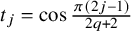 $t_j=\cos \frac {\pi (2j-1)}{2q+2}$
,
$t_j=\cos \frac {\pi (2j-1)}{2q+2}$
, $j=1,\dots ,q+1$
, are its zeros. If
$j=1,\dots ,q+1$
, are its zeros. If $x_i=\frac {\pi \nu _i}{2q+2}$
, then
$x_i=\frac {\pi \nu _i}{2q+2}$
, then
 $$\begin{align*}D(\nu)=D(\nu,\nu_m,\dots,\nu_1)=\det{}(\cos{}(2j-1)x_i)_{i,j=1}^{m+1}. \end{align*}$$
Since $\cos {}(2j-1)x_i=\sum _{s=0}^{j-1}c_{s}\cos ^{2s+1}x_i$
,
$\cos {}(2j-1)x_i=\sum _{s=0}^{j-1}c_{s}\cos ^{2s+1}x_i$
,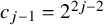 $c_{j-1}= 2^{2j-2}$
, the determinant
$c_{j-1}= 2^{2j-2}$
, the determinant $D(\nu )$
reduces to the Vandermonde determinant
$D(\nu )$
reduces to the Vandermonde determinant
 $$ \begin{align*} D(\nu)&=\det{}(2^{2j-2}(\cos x_i)^{2j-1})_{i,j=1}^{m+1}=2^{m(m+1)}\prod_{i=1}^{m+1}(\cos x_i)\det{}((\cos^{2}x_i)^{j-1})_{i,j=1}^{m+1}\\ &=2^{m(m+1)}\prod_{i=1}^{m+1}(\cos x_i)\prod_{1\le k<l\le m+1}(\cos^2x_l-\cos^2x_k)\\ &=2^{m(m+1)}\prod_{i=1}^{m+1}(\cos x_i)\prod_{1\le k<l\le m}(\cos^2x_l-\cos^2x_k)\,\prod_{1\le k\le m}\Big(\cos^2\Big(\frac{\pi\nu}{2q+2}\Big)-\cos^2\Big(\frac{\pi\nu_k}{2q+2}\Big)\Big). \end{align*} $$
Taking into account that $0<\cos x_1<\dots <\cos x_{m+1}<1$
, we obtain
$0<\cos x_1<\dots <\cos x_{m+1}<1$
, we obtain
 $$\begin{align*}\operatorname{sign} D(\nu)=\operatorname{sign} \prod_{k=1}^m \Big(\cos\Big(\frac{\pi\nu}{2q+2}\Big)-\cos\Big(\frac{\pi\nu_k}{2q+2}\Big)\Big)=\operatorname{sign} \prod_{k=1}^m(\nu_k-\nu). \end{align*}$$
(ii) The polynomial $U_{q+1}^{(0,1)}(t)$
is given by
$U_{q+1}^{(0,1)}(t)$
is given by
 $$\begin{align*}U_{q+1}^{(0,1)}(t)=P_{q+1}^{(-\frac{1}{2},\frac{1}{2})}(t)=\frac{\sqrt{2}\cos{}((q+3/2)\arccos t)} {\sqrt{1+t}} \end{align*}$$
and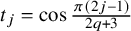 $t_j=\cos \frac {\pi (2j-1)}{2q+3}$
,
$t_j=\cos \frac {\pi (2j-1)}{2q+3}$
, $j=1,\dots ,q+1$
, are its zeros. If
$j=1,\dots ,q+1$
, are its zeros. If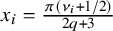 $x_i=\frac {\pi (\nu _i+1/2)}{2q+3}$
, then as above
$x_i=\frac {\pi (\nu _i+1/2)}{2q+3}$
, then as above
 $$ \begin{align*} D(\nu)&=\det \Big(\frac{\sqrt{2}\cos{}(2j-1)x_i}{\sqrt{1+t_j}}\Big)_{i,j=1}^{m+1}=\prod_{j=1}^{m+1}\Big(\frac{2}{1+t_j}\Big)^{1/2} \det \bigl(\cos{}(2j-1)x_i\bigr)_{i,j=1}^{m+1}\\ &=2^{m(m+1)}\prod_{j=1}^{m+1}\Big(\frac{2\cos^2 x_j}{1+t_j}\Big)^{1/2}\,\prod_{0\le k<l\le m+1}(\cos^2x_l-\cos^2x_k). \end{align*} $$
(iii) The polynomial
 $$\begin{align*}U_{q+1}^{(1,1)}(t)=P_{q+1}^{(\frac{1}{2},\frac{1}{2})}(t)=\frac{\sin((q+2)\arccos t)} {(q+2)\sqrt{1-t^2}}, \end{align*}$$
is the Chebyshev polynomial of the second kind with the zeros $t_j=\cos \frac {\pi j}{q+2}$
,
$t_j=\cos \frac {\pi j}{q+2}$
, $j=1,\dots ,q+1$
. If
$j=1,\dots ,q+1$
. If $x_i=\frac {\pi (\nu _i+1)}{q+2}$
, then
$x_i=\frac {\pi (\nu _i+1)}{q+2}$
, then
 $$\begin{align*}D(\nu)=\det \Big(\frac{\sin jx_i}{(\nu_i+1)\sin\frac{\pi j}{q+2}}\Big)_{i,j=1}^{m+1}= \frac{\det{}(\sin jx_i)_{i,j=1}^{m+1}}{\prod_{j=1}^{m+1}(\nu_j+1)\sin\frac{\pi j}{q+2}}. \end{align*}$$
Since $\sin jx_i=\sin x_i\,\sum _{s=0}^{j-1}c_{s}\cos ^{s}x_i$
with
$\sin jx_i=\sin x_i\,\sum _{s=0}^{j-1}c_{s}\cos ^{s}x_i$
with $c_{j-1}=2^{j -1}$
, we arrive at
$c_{j-1}=2^{j -1}$
, we arrive at
 $$ \begin{align*} D(\nu)&=2^{\frac{m(m+1)}{2}}\prod_{j=1}^{m+1}\frac{\sin\frac{\pi(\nu_j+1)}{q+2}}{(\nu_j+1)\sin\frac{\pi j}{q+2}}\,\det{}(\cos^{j-1}x_i)_{i,j=1}^{m+1}\\ &=2^{\frac{m(m+1)}{2}}\prod_{j=1}^{m+1}\frac{\sin\frac{\pi(\nu_j+1)}{q+2}}{(\nu_j+1)\sin\frac{\pi j}{q+2}}\, \prod_{0\le k<l\le m+1}(\cos x_l-\cos x_k). \end{align*} $$
(iv) We have
 $$\begin{align*}U_{q+1}^{(1,0)}(t)=P_{q+1}^{(\frac{1}{2},- \frac{1}{2})}=\frac{\sqrt{2}\sin((q+3/2)\arccos t)} {(2q+3)\sqrt{1-t}}, \end{align*}$$
and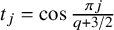 $t_j=\cos \frac {\pi j}{q+3/2}$
,
$t_j=\cos \frac {\pi j}{q+3/2}$
, $j=1,\dots ,q+1$
, are the zeros of
$j=1,\dots ,q+1$
, are the zeros of $U_{q+1}^{(1,0)}$
. As in the previous case, for
$U_{q+1}^{(1,0)}$
. As in the previous case, for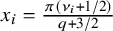 $x_i=\frac {\pi (\nu _i+1/2)}{q+3/2}$
,
$x_i=\frac {\pi (\nu _i+1/2)}{q+3/2}$
,
 $$ \begin{align*} D(\nu)&=\det \Big(\frac{\sqrt{2}\sin jx_i}{(2\nu_i+1)\sqrt{1-t_j}}\Big)_{i,j=1}^{m+1}= \frac{\det{}(\sin jx_i)_{i,j=1}^{m+1}}{\prod_{j=1}^{m+1}(2\nu_j+1)\sqrt{(1-t_j)/2}}\\ &=2^{\frac{m(m+1)}{2}}\prod_{j=1}^{m+1}\frac{\sin\frac{\pi(\nu_j+1)}{q+2}}{(2\nu_j+1)\sqrt{(1-t_j)/2}}\prod_{0\le k<l\le m+1}(\cos x_l-\cos x_k). \end{align*} $$
A.2 Corollaries of Theorem 1.14 for trigonometric polynomials
Finally, writing the Chebyshev polynomials $U_{q+1}^{(0,0)}$
and
$U_{q+1}^{(0,0)}$
and $U_{q+1}^{(1,1)}$
in the trigonometric form, the monotonicity property of coefficients in expansion (1.15) given in Theorem 1.14 implies the following results.
$U_{q+1}^{(1,1)}$
in the trigonometric form, the monotonicity property of coefficients in expansion (1.15) given in Theorem 1.14 implies the following results.
Corollary A.1. Suppose $0\le m\le q$
, then
$0\le m\le q$
, then
 $$ \begin{align} \frac{\cos{}(q+1)x}{\bigl(\cos x-\cos\frac{\pi}{2q+2}\bigr)\cdots\bigl(\cos x-\cos\frac{\pi(2m+1)}{2q+2}\bigr)}= \frac{a_{0,m}}{2}+\sum_{\nu=1}^{q-m}a_{\nu,m}\cos\nu x, \end{align} $$
then
 $$\begin{align*}a_{0,m}>a_{1,m}>\dots>a_{q-m,m}>0. \end{align*}$$
Corollary A.2. Suppose $1\le m\le q$
, then
$1\le m\le q$
, then
 $$\begin{align*}\frac{\sin(q+1)x}{\bigl(\cos x-\cos\frac{\pi}{q+1}\bigr)\cdots\bigl(\cos x-\cos\frac{\pi m}{q+1}\bigr)}= \sum_{\nu=1}^{q-m+1}\nu b_{\nu,m}\sin\nu x, \end{align*}$$
then
 $$\begin{align*}b_{1,m}>\dots>b_{q-m+1,m}>0. \end{align*}$$
It is worth mentioning that polynomials similar to (A.1) were considered by Yudin in [Reference Yudin40].
Acknowledgements
We would like to thank the anonymous reviewers for their valuable and constructive comments, which allowed us to significantly improve the article.
Competing interest
The authors have no competing interests to declare.
Funding statement
The proofs of Theorems 1.4, 1.8, 1.10, 1.14 were supported by the Russian Science Foundation (project no. 23-71-30001) at the Lomonosov Moscow State University. The work of the third author was partially supported by grants PID2023-150984NB-I00, 2021 SGR 00087, the CERCA Programme of the Generalitat de Catalunya, and by the Spanish State Research Agency, through the Severo Ochoa and María de Maeztu Program for Centers and Units of Excellence in R $\&$
D (CEX2020-001084-M).
$\&$
D (CEX2020-001084-M).
Author contributions
All authors contributed equally to this work.





 Open access

