


1. Introduction
Antarctic mass balance is challenging to measure and predict, which directly impacts current estimates of sea-level rise and future projections (Fürst and others, Reference Fürst2016; IMBIE team, Reference IMBIE team, Shepherd and Ivins2018; Lenaerts and others, Reference Lenaerts, Medley, van den Broeke and Wouters2019). In the Antarctic coastal regions, ice–ocean interactions, surface mass balance (SMB) and buttressing from locally grounded ice rises and rumples all affect ice shelf mass balance, which has a major control on mass discharge from the ice sheet through the grounding line (Matsuoka and others, Reference Matsuoka2015). SMB is often estimated using regional climate models or satellite observations of passive microwave, which have a spatial resolution of tens of kilometers in most cases (Lenaerts and others, Reference Lenaerts2017; van Wessem and others, Reference van Wessem2018). This is not sufficient to capture the finer scale topography of ice rises and rumples which induce considerable local variations in SMB (Lenaerts and others, Reference Lenaerts2014; Wang and others, Reference Wang2016; Kausch and others, Reference Kausch2020). Given the high rates of SMB and its high-spatial variability due to local topographic variations at these locations, regional SMB estimates are poorly constrained. Detailed observational constraints are necessary in order to evaluate and improve regional climate models.
The coastal region of Dronning Maud Land (DML) in East Antarctica is characterized by numerous small ice shelves bounded between distinct topographic features (i.e. ice rises) with their own specific local flow, climate regime and spatially varied SMB (Lenaerts and others, Reference Lenaerts2014; Rignot and others, Reference Rignot2019; Goel and others, Reference Goel2020). The specific local flow regime typically consists of the ice flowing from stationary ice dome of the ice rise toward the ice shelf. Both snowfall and re-distribution of snow by wind are largely controlled orographically at various spatial scales across the ice shelves and ice rises (King and others, Reference King2004; Favier and Pattyn, Reference Favier and Pattyn2015; Matsuoka and others, Reference Matsuoka2015; Callens and others, Reference Callens, Drews, Witrant, Philippe and Pattyn2016; Kausch and others, Reference Kausch2020). SMB characteristics near the ice-rise summits are of particular interest since ice rises are close to the ocean and SMB is often much larger than inland sites giving higher temporal resolutions in the paleoclimate proxies over the past several millennia. Spatially resolved SMB at sub-decadal periods are needed to understand recent ice-rise and ice-shelf dynamics, but such ground-penetrating radar (GPR)-based records are very limited in DML (Lenaerts and others, Reference Lenaerts2014; Callens and others, Reference Callens, Drews, Witrant, Philippe and Pattyn2016; Goel and others, Reference Goel, Brown and Matsuoka2017).
Here, we present SMB variations along an across-flow, eastwest transect over a small ice shelf in central DML, the Nivlisen Ice Shelf, and its adjacent Leningradkollen and Djupranen ice rises over the past three decades. SMB is constrained by shallow radar reflectors dated with ice cores collected at these ice rise summits (Fig. 1). Previous SMB studies of the Nivlisen Ice Shelf have been limited to short-term stake measurements in limited areas (Horwath and others, Reference Horwath2006; Lindbäck and others, Reference Lindbäck2019). The primary goal of the study is to reveal spatial and temporal SMB of the ice rises and the ice shelf. We analyzed the SMB results in relation to surface topography (i.e. elevation) and compared with SMB estimated with a regional climate model.
The Nivlisen Ice Shelf, central DML coast. The location of the main map is shown in the inset. Shallow radar profiles collected in 2016/17 (brown) and 2017/18 (blue) connect to the two ice-core sites at the summits (yellow stars) of the Leningradkollen and Djupranen ice rises. Surface density was measured with 3 m firn cores at 14 locations (red dots) and SMB between 2017 and 2018 were measured at stakes (black dots). A dense GNSS survey (thin gray lines) was made on each ice rise. The background image is the Landsat Image Mosaic of Antarctica taken between 1999 and 2003 (Bindschadler and others, Reference Bindschadler2008), with grounding line (Mouginot and others, Reference Mouginot, Scheuchl and Rignot2017), ice shelf fronts and ice surface features digitized from Radarsat-2 imagery taken between 2012 and 2014 (Goel and others, Reference Goel2020), and surface elevation (m a.s.l.) contours over the grounded ice (Howat and others, Reference Howat, Porter, Smith, Noh and Morin2019). Coordinate reference system: WGS84 Antarctic polar stereographic parallel to 71° S (EPSG: 3031). This map is made using Quantarctica (Matsuoka and others, Reference Matsuoka2021).

2. Study area
The Nivlisen Ice Shelf covers ~10 400 km2 of area, extending ~80 km in the southnorth direction along the ice flow and 130 km in the eastwest direction between two promontory-type ice rises (Fig. 1). Ice thickness along the eastwest transect ranges between 210 and 330 m, with the thickest ice in the central part (Lindbäck and others, Reference Lindbäck2019). The Nivlisen Ice Shelf is mainly fed by the Potsdam Glacier. The summits of the two ice rises, Leningradkollen (east) and Djupranen (west) have surface elevations of 174 and 321 m a.s.l., respectively. Climatically, the region receives moisture and precipitation from an easterly wind flow, however, the accumulation rate and snowfall distribution are modified by the elevated topography bringing higher precipitation on the upwind sides (Lenaerts and others, Reference Lenaerts2013). The Nivlisen Ice Shelf has a series of small ice rumples and rises near the present ice front and flows with an average speed of ~80 m a−1, which is slower than the adjacent ice shelves that have no ice rises and rumples near the calving front (Rignot and others, Reference Rignot, Mouginot and Scheuchl2011). These rumples and ice rises can provide backstress to the ice shelf (Fürst and others, Reference Fürst2016), and loss of these pinning points might destabilize the ice shelf and upstream ice sheet (Favier and Pattyn, Reference Favier and Pattyn2015).
3. Instrumentation and data
We collected field data during two campaigns in 2016/17 and 2017/18 austral summers.
3.1. Kinematic GNSS survey for topography
We made differential kinematic Global Navigation Satellite System (GNSS) surveys using Trimble NetR9 dual-frequency receivers over the two ice rises to measure their surface topography (Fig. 1). Two base stations were set up near the ice-coring site at the ice-rise summits. Rover receivers were installed on each snowmobile moving at a nominal speed of 15 km h−1. The survey was conducted in a grid pattern with typical spacing between two adjacent profiles of 1–2 km. Data were collected at 1 s intervals, giving the nominal data spacing of ~4 m along the profile. Kinematic baselines between the base station and the rovers were analyzed using Trimble software and the base station positions were fixed with a Canadian precise point-processing service (CSRS-PPP; Natural Resources Canada, 2017). To derive the elevations relative to the mean sea level, we used the EGM2008 geoid model (Pavlis and others, Reference Pavlis, Holmes, Kenyon and Factor2012).
3.2. Radar profiling and reflector dating
Shallow englacial stratigraphy was observed using a 250-MHz pulseEKKO GPR for ~145 km profile length over the Leningradkollen Ice Rise in 2016/17 austral summer, and ~85 km over the Djupranen Ice Rise and ~160 km over the Nivlisen Ice Shelf in 2017/18 austral summer (Fig. 1). The radar system was towed behind a snowmobile at a speed of 12–15 km h−1. Geographic locations of the GPR data were acquired using a GNSS receiver connected to the system. Radar data were digitized at 0.4 ns intervals over a time window of 500 ns, corresponding to the top ~45 m of the firn with a radio-wave propagation speed of 0.2 m ns−1 sampled at ~4 cm depth intervals. Four waveforms were averaged to reduce thermal noise so that the data were recorded with ~1.3 m intervals along the radar profiles. Post-processing to develop radargrams includes a Dewow filter, band-pass filter and depth-variable gain function (e.g. Goel and others, Reference Goel, Brown and Matsuoka2017). Radar profiles were made 30–100 m away from the ice-core sites to prevent radar scatters from the ice-coring set-up.
To estimate the spatial and temporal patterns of SMB using the GPR data, we first identified five to six prominent reflectors (assumed to be isochrones) and tracked them along all the profiles collected over the ice rises and ice shelf individually. Two ice cores drilled at the summits of the Djupranen and Leningradkollen ice rises during 2016/17 austral summer were used to date the reflectors (Fig. 2). The Leningradkollen ice core is 50 m long, whereas the Djupranen ice core is 122 m long. Chronology for the ice cores was established by annual layer counting using seasonal cycles in δ18O data and snow/firn layering through high-resolution visual stratigraphic techniques. Furthermore, independent age constraints were obtained using markers of historically known volcanic eruptions such as Pinatubo (1993) and Agung (1963), identified in the ice cores by anomalous sulfate peaks. Bulk density was measured up to a depth of 35 m and varied between 436 and 739 kg m−3 (Figs 2a, d).
Ice-core data used to constrain the depth and age of radar reflectors, collected at the Djupranen (top row) and Leningradkollen (bottom row) ice rises. (a, d) Depth profile of measured density used to calculate depth profile of radio-wave propagation speed (black) shown in (b, e) as well as from the firn-densification model (Herron and Langway, Reference Herron and Langway1980; H&L) shown by the red curve constrained with ice-core data. (c, f) Depth profiles of age constrained by ice-core data. Dotted lines show the correspondences between depths of six tracked radar reflectors and their ages.

To compensate for the snow surface changes between the time of ice coring in 2016/17 and the time of radar data collection in 2017/18 over the ice shelf and the Djupranen Ice Rise, we added surface height difference measured using a snow stake at both the ice-core site between 2016/17 and 2017/18 seasons to the ice-core data, so that radar data over the Djupranen Ice Rise and the Nivlisen Ice Shelf are referenced to the 2017/18 snow surface. Therefore, the SMB for the Leningradkollen Ice Rise is before 2016, and SMB for the Nivlisen Ice Shelf and the Djupranen Ice Rise is prior to 2017.
We accounted for depth-variable radio-wave propagation speed (v) using density data measured with the ice cores and using the equation from Kovacs and others (Reference Kovacs, Gow and Morey1995):

where z is the depth, c is the speed of light in a vacuum (0.30 m ns−1) and ρ(z) is a depth-dependent density from the ice core. The measured densities from both the ice cores are in good agreement with a firn densification model (Herron and Langway, Reference Herron and Langway1980; Figs 2a, d). Assuming that ice core measured densities do not vary spatially, we used the Leningradkollen ice-core density curve (Figs 2d–f) to date and calculated mass from reflectors observed over the Nivlisen Ice Shelf and the Leningradkollen Ice Rise, whereas we used the Djupranen ice-core density curve for the reflectors over the Djupranen Ice Rise. We examine the uncertainty of different density curves obtained at the core sites in Section 5.1.
Each reflector's depth (z) at a given point was estimated from the two-way propagation time t(z) and the depth-dependent propagation speed v(z) obtained with Eqn (1):

After converting travel time to depth, the mass of ice in each layer between two reflectors is derived using the density curves (Fig. 2) and then divided by the age difference between these two reflectors (e.g. Waddington and others, Reference Waddington, Neumann, Koutnik, Marshall and Morse2007). Here, we assume that the reflector depths do not change over the 30–100 m distance between the core sites and the closest radar data points.
3.3. Snow stakes
We also measured the annual SMB between the two field campaigns in 2016/17 and 2017/18 austral summer using fixed snow stakes. We installed 23 aluminum stakes and drilled 3 m firn cores at 11 of these sites over the ice rises and the ice shelf (Fig. 1). The snow surface is smooth in most areas, but micro-topography including sastrugi is more prominent over western, downwind, sides of the ice rises. For such case, we tried to install the markers to a representative surface in its vicinity. In the top 1 m, snow density varied between 430 and 450 kg m−3 at these locations, and we used its mean of 440 kg m−3 to estimate the SMB from the stake height changes over the year, assuming that these stakes did not move relative to the snow surface.
4. Results
4.1. Surface topography and snow-surface conditions
The dense GNSS kinematic surveys revealed details of the topography of the two ice rises (Fig. 3a). The Djupranen Ice Rise has a ridge from the ice sheet to the seaward ice dome. The ice rise summit is 321 m a.s.l. and elevated by ~90 m from the saddle between the dome and the landward ridge. The Leningradkollen Ice Rise has a more complex topography. In addition to the seaward dome (174 m a.s.l.), which is elevated by ~65 m from the saddle between the dome and the landward ridge, there is another ridge from the dome to the west. Its elevation decreases steeply by 25 m within 4 km, followed by a flatter ridge with ~10 m elevation variation over 10 km to the western end.
Firn stratigraphy detected with 250 MHz radar frequency. (a) Location of the radar profile in panel (b) shown together with ice surface features (Goel and others, Reference Goel2020) and surface elevations of 20 m contour intervals reconstructed from the GNSS survey over the ice rises. Continental grounding line and ice rise outline were taken from Bindschadler and others (Reference Bindschadler2011) and Moholdt and Matsuoka (Reference Moholdt and Matsuoka2015), respectively. Pink markers show the distance from Leningradkollen core site along the profile. The background image is a hill-shade extracted from the REMA (Howat and others, Reference Howat, Porter, Smith, Noh and Morin2019). (b) Radargram across the ice shelf between the ice-core sites at the summits of the two ice rises. The down-pointing arrows show the grounding line positions (GL; Bindschadler and others, Reference Bindschadler2011). Close up views of the profiles between the core sites and GL regions are shown in panels (c) and (d). Blue dots indicate the six reflectors tracked and dated using the ice cores (Figs 2c, f).

We evaluated the Reference Elevation Model of Antarctica (REMA) Digital Elevation Model (DEM) of Antarctica at 8 m spatial resolution (Howat and others, Reference Howat, Porter, Smith, Noh and Morin2019) using the GNSS profile data over the ice rises. First, we interpolated the REMA DEM to all GNSS survey points using four neighboring DEM cells. A histogram of the differences between these interpolated REMA DEM elevations and the GNSS survey elevations show a main peak near the zero difference, although a smaller peak also exist at a difference of ~3 m. The latter is associated with a few GNSS profiles and these were rejected from further analysis. Excluding these outliers, the mean and std dev. of the elevation differences between REMA DEM and GNSS survey are 0.21 ± 0.64 m at the Leningradkollen and 0.74 ± 0.64 m at Djupranen ice rises.
For both the Djupranen and Leningradkollen ice rises, we found that the surface was smooth on the eastern side, whereas it was rough on the western side. The surfaces in the northern and southern slopes of the eastwest ridge of Leningradkollen are also distinct; rough surface in the northern slope facing to the ocean, and smoother surface in the southern slope.
4.2. GPR stratigraphy
The radar data clearly show stratigraphy almost all along the radar profiles, both over the ice shelf and ice rises (Fig. 3b). Englacial reflectors along the 160 km long profile between the two ice-core sites have numerous undulations over short distances, and such undulations are more significant at locations toward the middle of the ice shelf where several ice-flow stripes are present (Figs 3a, b). The upper portion of the Nivlisen Ice Shelf experiences extensive surface melting in summer, and meltwater features advect downstream with the ice shelf (e.g. Kingslake and others, Reference Kingslake, Ely, Das and Bell2017). However, these melt features are located a few tens of kilometers upstream of our radar profile, and the ice shelf moves <100 m a−1 in this region (Rignot and others, Reference Rignot, Mouginot and Scheuchl2011). We did not observe major stratigraphic disturbance caused by meltwater in the radargrams (Fig. 3). On the eastern side (20–60 km from the Leningradkollen core site), the reflectors are relatively smooth with little variation in depth. However, the reflectors become deeper toward the western end of the ice shelf (>70 km).
We tracked six reflectors from the Leningradkollen ice-core site toward the ice shelf. The reflectors are down-warped for ~1 km near the grounding line. Here, we also observe small surface cracks. Nonetheless, radar reflectors are still traceable (Fig. 3d). These reflectors deepen toward the west, so the deepest three reflectors fall outside the radar's depth window at locations of ~70–140 km west of Leningradkollen (Fig. 3b). At the Djupranen grounding line (Fig. 3c), the reflector down-warping is more pronounced than at the Leningradkollen grounding line, and it was not possible to confidently track the top three reflectors across the grounding line. Here, we observed crevasses that are ~40 m deep and 2–3 m wide, which we needed to fill with snow to continue our over-snow traverse to the Djupranen Ice Rise.
The six reflectors tracked along the transect were dated as 3.7, 6.9, 11.3, 17.6, 23.7 and 30.9 years before December 2017 using the Leningradkollen ice core (Fig. 2f). Because the reflectors are not readily traceable over the Djupranen grounding line (Fig. 3c), we picked up similarly prominent reflectors at the ice-rise side of the grounding line and tracked them to the Djupranen ice-core site. These three reflectors are dated as 5.5, 7.1 and 12.2 years before December 2017 using the Djupranen ice core (Fig. 2c). As there are no other reflectors close to these depths that can be tracked for long distances from this grounding line, we argue that these three reflectors are identical to those tracked from the Leningradkollen Ice Rise. In that case, the difference in ages of these reflectors (0.2–1.8 years) may be associated with uncertainties in ice-core chronology and in radar reflector tracking, which are discussed in Section 5.1. We picked three more reflectors over the Djupranen Ice Rise, which are dated as 20.4, 25.4 and 27.4 before December 2017. Separately, we tracked five reflectors over the Leningradkollen Ice Rise that dated as 4.5, 8.3, 14.9, 19.7 and 29.3 years before December 2016. These reflectors give the best clarity and extent over the ice rises where the snow depositional conditions are much more variable than on the ice shelf.
4.3. SMB derived from radar data
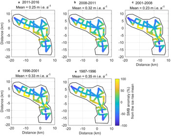
SMB over the Nivlisen Ice Shelf and the Leningradkollen and Djupranen ice rises are shown in Figures 4, 5 and 6, respectively. Their spatial anomalies are presented in Figures 7, 8 and 9, respectively. Temporal changes of the spatial means of these regions are shown in Figure 10 and summarized in Table 1.
SMB and elevations across the Nivlisen Ice Shelf. (a) SMB for six periods derived from the radar data and SMB for 2016/17 measured with stakes. The horizontal axis shows the distance from the Leningradkollen ice-core site (i.e. 0 km). Vertical gray shades represent the Leningrad and Djupranen grounding line positions. SMB cannot be derived for ~1 km at the latter. (b) Surface elevations measured with kinematic GNSS survey were corrected for the tides (Padman and others, Reference Padman, Erofeeva and Joughin2003) and geoid heights using the EGM2008 geoid model (Pavlis and others, Reference Pavlis, Holmes, Kenyon and Factor2012). Also shown is a DEM profile used as a boundary condition of the RACMO regional climate model. Detailed GNSS elevation variations over the ice shelf along the same profile are shown in blue curve with the right axis.

Overview of the spatial SMB variability relative to the mean SMB for the Leningradkollen Ice Rise during five different time periods. The mean annual SMB for each period is given above each panel and listed in Table 1.

Overview of the spatial SMB variability relative to the mean SMB for the Djupranen Ice Rise during six different time periods. The mean annual SMB for each period is given above each panel and listed in Table 1.

Spatial anomalies of SMB from the ice-shelf-wide mean SMB (Table 1) for the six time periods. (a) Radar-derived SMB. (b) SMB modeled with RACMO2.3p2. Mean model values used to derive model anomalies are calculated for the regions where radar-derived SMB values are available for the corresponding periods. Note that curves for 1986–93 in RACMO2.3p2 appear above all the other curves, although SMB for this period is lowest (Table 1; Fig. 10).

Overview of SMB anomaly over five periods (a–e), and ice-surface topography of the Leningradkollen Ice Rise (f). (a–e) Stripes show radar-derived SMB and background shows model-derived SMB, both as percentage anomalies from each ice-rise mean. (f) Ice surface elevation interpolated from GNSS survey (red lines).

Overview of SMB anomaly (a–f) and ice-surface topography (g) of the Djupranen Ice Rise. (a–f) Stripes show radar-derived SMB and background shows model-derived SMB, both as percentage anomalies from each ice-rise mean. (g) Ice surface elevation reconstructed from GNSS survey (red lines).

SMB changes in the past three decades over (a) the Nivlisen Ice Shelf, (b) the Leningradkollen Ice Rise and (c) the Djupranen Ice Rise. In each panel, red lines show radar-derived SMB, and blue lines show RACMO2.3p2 modeled SMB (RACMO data are available only until 2015), both averaged over these regions. Black lines in panels (b) and (c) show SMB at the ice-rise summits derived from the ice cores. Dashed horizontal lines show the mean over the entire period obtained from these three methods.

Summary of the regional mean SMB derived with the radar data for the last three decades

Mean of RACMO2.3p2 SMB values are also shown for comparison. The radar-derived SMB values shown with * are derived only in a limited area of each region. RACMO results are available only until 2015, which are shown with # in the table. Nominal uncertainty of radar-derived SMB is ±11%.
4.3.1. The Nivlisen Ice Shelf
We used the Leningradkollen ice core to date the reflectors over the ice shelf and derived SMB for six periods during the last 31 years; 2013–17, 2010–13, 2006–10, 1999–2006, 1993–99 and 1986–93. We excluded the vicinity of the Djupranen grounding line from the SMB estimate because radar reflectors are down-warped there for a distance of ~1 km, which is more likely associated with observed crevasses there (Fig. 4). Except for the earliest period (1986–93), all other SMB profiles show similar spatial patterns. First, SMB stays relatively low between the Leningradkollen grounding line to ~60 km along the profile. Second, from ~60 km to the Djupranen grounding line, SMB increases gradually with some local fluctuations. The magnitude of this increase differs between periods; SMB increases by a factor of 1.6 for the most recent period 2013–17, 1.5 for 2010–13, 2.0 for 2006–10, 1.7 for 1999–2006 and 1.6 for 1993–99. Local SMB undulations of 0.1–0.2 m ice equivalent a−1 (hereafter, m i.e. a−1) over 100–500 m distances were found at the same locations regardless of the periods.
Over the profile across the ice shelf between the two grounding lines, the region-wide mean SMB was found to be in the range from a minimum of 0.37 m i.e. a−1 for 2010–13 to a maximum of 0.84 m i.e. a−1 for 1986–93 (Table 1). The SMB over the Nivlisen Ice Shelf during the 2016–17 period measured at 14 stakes varies from 0.12 in the east to 0.62 m i.e. a−1 in the west, with a mean value of 0.37 m i.e. a−1. These values are broadly consistent with radar-derived SMB over the most recent period (2010–17). Four stakes spanning 40 km on the eastern side (10–50 km in Fig. 4) show lower SMB than the radar-derived SMB over the most recent period.
4.3.2. Ice rises
Over the Leningradkollen Ice Rise, SMB was derived using the five reflectors spanning periods of 3–9 years between 1987 and 2016. Mean SMB over the ice rise ranges between 0.23 and 0.35 m i.e. a−1 over the five periods, whereas the spatial variability of SMB is large but relatively stable between periods (Fig. 5). Lower SMB is found in the northern slope of the eastwest ridge, and the northeast side of the ice dome. There, SMB is only one-quarter of the ice-rise mean values. Correspondingly, higher SMB values were found in the southern slope of the eastwest ridge, and the saddle between the seaward dome and the landward promontory. Across the eastwest ridge, SMB varies by more than ±50% of the ice-rise mean within 10 km from the northern side facing the open ocean to the southern side facing the ice-shelf inlet.
At the Djupranen Ice Rise, we estimated SMB over six periods spanning 2–9 years between 1990 and 2017 (Fig. 6). The regional-mean SMB over the Djupranen Ice Rise varies between 0.38 and 0.64 m i.e. a−1 over these periods, which is much larger than temporal variations of ice-rise mean SMB observed over the Leningradkollen Ice Rise (Table 1). Anomalously high SMB is found near the grounding line east of the ice rise, which is the upwind side. Except for this, the spatial patterns over the Djupranen Ice Rise are less persistent over time than those over the Leningradkollen Ice Rise. For example, high SMB is observed near the western, downwind grounding line for a few periods, but not for all periods. Similarly, SMB along the ridge from the seaward dome to the ice sheet is smaller for a few periods, but not for all periods. SMB for the 1990–92 periods is estimated only in small areas over the ice rise because the deepest reflector dated at 1990 deepens out of the radar window (to the depth ~35 m). In general, the ice rise has an east to west SMB contrast. The SMB over the eastern side of the ice rise is ~50–100% higher than the ice-rise mean.
5. Discussion
We first discuss uncertainties associated with stake-based and radar-derived SMB measurements. Then, we evaluate the topographic controls on the spatial SMB patterns and present the findings in context to previous study in the region. Finally, we compare the observed SMB with high-resolution (5.5 km) RACMO2.3p2 ANT/DML SMB (hereafter RACMO2.3p2) estimates from 1986 to 2015 (Lenaerts and others, Reference Lenaerts2017; van Wessem and others, Reference van Wessem2018), and evaluate how accurately the model can capture SMB variations over various spatial scales.
5.1 SMB uncertainty due to variable firn density and densification
Uncertainties associated with stake-derived SMB are from near-surface density and stake height measurements. Surface density (mean in the top 1 m) measured at 11 sites varies between 430 and 450 kg m−3, or ±5%. The uncertainties in core diameter (±0.1 cm), core-length measurements (±0.3 cm) and weight measurement (±5 g) result in propagated uncertainty of 4% in density of a 1 m snow core. Uncertainty of the stake heights is <±1 cm or 1.2% of the mean height difference. Although we chose representative surface in its vicinity to install the markers, but local variability of SMB associated with microtopography cannot be evaluated. Therefore, stake-measured SMB has an uncertainty better than ±5%.
Uncertainty in the radar-derived SMB values are related to uncertainties in ice-core density and chronology, and uncertainties in the two-way travel time of reflectors. The density of the ice-core samples was measured in a cold room; the error in measuring the dimensions (5 cm × 5 cm × 3.5 cm) of the samples was ±0.5 mm and the uncertainty of the weighing balance was ±0.1 g for measured mass up to 100 g of snow/firn. It results in a propagated uncertainty of 5% in the ice-core density measurements. For the top 15 m snow/firn column of ice core, the uncertainty in chronology using independent methods is ±1 year, calculated as the difference between the minimum and maximum age estimates at a particular depth point. This is supplemented by the observation that the ages of the three shallowest reflectors dated by the two ice cores differ by 1.8, 0.2 and 0.9 years. This uncertainty affects the magnitude of SMB for corresponding periods but does not affect the spatial patterns of SMB.
Another uncertainty in the radar-derived SMB values is from the assumption of laterally uniform density. We assume that the density varies with depth as observed in the Djupranen ice core but does not vary laterally. We examined this assumption in two ways. First, we used Djupranen (instead of Leningrad) ice-core density to calculate depths of tracked reflectors, assign the new ages of these reflectors using the Leningrad or Djupranen ice cores (as we did in the primary analysis), and calculate SMB using the Djupranen (instead of Leningrad) ice-core depth density data. As Figure 2 shows, density profiles from the two ice rise summits are similar and have no systematic bias to each other; the density difference between the two cores at a given depth is 25 kg m−3 on average, and the std dev. of this difference is ±46 kg m−3. This brings an uncertainty of 5% between two ice-core densities. The radio-wave propagation speed averaged from the surface to 10 m depth derived with the Djupranen density differs by 1.4% from our original estimate. However, this variation in the radio-wave propagation speed causes no change in the age estimate from the original ages. As a consequence, we found similar SMB for all reflectors with no change in spatial patterns. Second, we examined variations of density between the surfaces to 3 m depth measured with shallow snow/firn cores of 3 m at 14 locations (see Fig. 1 for these core locations). The surface density to 3 m ranges from 465 kg m−3 at the Leningradkollen Ice Rise summit to 505 kg m−3 at the western side of the Djupranen Ice Rise with a mean and std dev. of 484 ± 12 kg m−3. The surface density over the ice shelf at four locations has mean and std dev. values of 483 ± 7 kg m−3.
To evaluate the uncertainty in reflector tracking, we carried out cross-over analysis. There are 15 cross-over sites over the Leningradkollen Ice Rise, and three sites over the Djupranen Ice Rise, whereas the ice shelf has no cross-over profile. At these 18 locations, the mean cross-over error is 1.0 ns (or ~10 cm in firn) with a std dev. of 0.4 ns (4 cm). This mean cross-over error constitutes 6% of the depth uncertainty for the shallowest reflector but the relative magnitude is smaller for deeper reflectors.
Combining the sources of uncertainty that we are able to estimate as a root-sum-square, an uncertainty of ±11% was determined for the radar-derived SMB estimates. Local SMB uncertainties might be higher than this due to unaccounted density variations in areas such as the ice shelf margins and the high-accumulation zone near Djupranen.
5.2 Spatial SMB pattern
The Antarctic coast is characterized by varying surface topography that interacts with wind and moisture to promote precipitation and snow redistribution, resulting in an inhomogeneous distribution of SMB (Lenaerts and van den Broeke, Reference Lenaerts and van den Broeke2012; Rignot and others, Reference Rignot2019). Elevation differences between ice shelves and ice rises play an important role in controlling spatial SMB distribution in the coastal DML region (Lenaerts and others, Reference Lenaerts2014; Drews and others, Reference Drews2015; Goel and others, Reference Goel, Brown and Matsuoka2017). We found a strong eastwest SMB gradient over the Nivlisen Ice Shelf with local variations being 1–2 orders of magnitude smaller than the regional variation. This eastwest SMB difference is large and monotonic, which is presumably caused by a strong regional orographic effect of the Leningradkollen and Djupranen ice rises, similar to those observed at other Antarctic ice rises (King and others, Reference King2004; Lenaerts and others, Reference Lenaerts2014).
Although large-scale surface topography dominates SMB variations, notable small scale <500 m SMB undulations were also observed (Fig. 4). These undulations have SMB amplitudes of 0.05–0.2 m i.e. a−1 over a length of 500 m. The eastwest profile over the ice shelf crosses along-flow stripes seen in satellite imagery (Fig. 1), and ice surface depressions of 4–7 m were also observed at many of these locations at the downstream of mid-ice shelf rumples spread over 10 km along the profile at 60–120 km from the Leningradkollen Ice Rise (Fig. 4). Local SMB anomalies have been observed over similar local topographic features in other parts of Antarctica (Drews and others, Reference Drews2015; Drews and others, Reference Drews2020; Kausch and others, Reference Kausch2020). In an attempt to explore small-scale variations, we determined local anomalies in SMB together with surface elevation. We found a spatial correspondence between the resulting surface and SMB anomalies, with surface undulations of 10–25 cm leading to SMB variations within 5–15 mm i.e. a−1. However, as the scale of these variations is within the uncertainty range of these data, conclusive inferences cannot be made. The SMB variations on the ice rises are more complex but relatively stable over time which indicates persistent climate conditions with respect to surface topography, at least for the Leningradkollen Ice Rise. At the larger scale, both ice rises act as wind barriers against the dominating easterly winds, with the majority of the precipitation coming from northeasterly storms.
5.3 Comparison with a regional climate model
Regional atmospheric climate models often have a spatial resolution of tens of kilometers, which is typically too coarse to fully resolve individual ice rises along the coast. Along the DML coast, the regional climate model RACMO2.3p2 ANT/DML is available with a spatial resolution of 5.5 km from 1979 to 2015 (Lenaerts and others, Reference Lenaerts2017). This model resolves most of the promontories and several isle ice rises, although their surface topography is coarsely prescribed (Fig. 4b).
To compare the observed and modeled SMB, we derived a distance-weighted mean of modeled SMB at each radar point using the model's four closest cells. RACMO2.3p2 SMB could be extracted for all radar SMB periods except that RACMO2.3p2 only extends to the end of 2015. Figure 7 shows that the large-scale eastwest trend over the ice shelf is well represented by the model. However, the eastwest contrast according to the model is larger than the observations; the radar-derived SMB varies by ~200% (i.e. −50 to +150%), whereas RACMO SMB varies by 290% (−70 to +220%).
For the Djupranen Ice Rise we obtained a total of 55 RACMO2.3p2 gridcells, and for the Leningrad Ice Rise we obtained a total of 33 gridcells (Figs 8 and 9). The RACMO2.3p2 SMB indicates consistently lower SMB on the leeward (western) side, whereas the radar-derived SMB show more complex patterns and smaller-scale variability.
The RACMO2.3p2 model has a 5.5-km cell size, so any orographic effect is modeled only for approximated topography, which could be the main cause of discrepancies between modeled and observed SMB patterns. Therefore, we next compared SMB values averaged over the ice shelf and each ice rise (Fig. 10 and Table 1). These regional mean values are derived from all measured SMB values and all modeled SMB values constructed at the radar-observation locations. Ice-core SMB represents only the vicinity of the ice rise summit. When these mean values are averaged over the entire period, modeled SMB values are smaller than radar-derived SMB values over the ice shelf and the Leningradkollen Ice Rise by ~20–50%. Modeled SMB values are smaller than radar-derived SMB values for most of the individual periods, but the magnitude is different. Over the Djupranen Ice Rise, modeled SMB values are larger than radar-derived values, but <20% different. This magnitude relation remains the same for individual periods in most cases. Furthermore, the ice-core SMB values are 50–80% smaller than the radar-derived and modeled SMB for both ice rises. A large temporal variability has been observed among all SMB observations, which has been explained mainly by topographic differences of the ice rises and the surrounding ice shelf (Kausch and others, Reference Kausch2020). We found that the ice-core records from the ice-rise summits do not necessarily represent ice-rise-wide SMB changes, and also climate models do not match either the core-based SMB at the summits or radar-derived SMB over the ice rise.
6. Conclusions
We carried out GPR and GNSS surveys to measure spatial variations in SMB over the last three decades and ice topography of the Nivlisen Ice Shelf and the adjacent two ice rises. For both ice rises, we found that the surface was smooth on the eastern windward side, whereas it was rough on the western leeward side. There is a strong spatial SMB gradient between low SMB in the inlet of the ice shelf facing to the Leningradkollen Ice Rise (0.25 m i.e. a−1) and high SMB in the west toward the more elevated Djupranen Ice Rise (0.75 m i.e. a−1) for the most recent periods 2010–17. This eastwest pattern was maintained for the entire observational period of the last three decades (1986–2017), but the eastwest contrast in SMB varies by a factor of 1.5–2 depending on the periods. The ice rises have their own contrasting SMB patterns owing to distinct ice rise topographies. The spatial-mean SMB over the Leningradkollen Ice Rise was 0.30 m i.e. a−1 between 1987 and 2016, whereas the spatial-mean SMB over the Djupranen Ice Rise was 0.51 m i.e. a−1 during 1990–2017. The comparison of radar-derived SMB with modeled SMB from RACMO2.3p2 at 5.5 km resolution shows that the model can capture the main gradient across the ice shelf, but is prone to topographically related SMB biases on the ice rises. Model estimates of SMB do not match the regional-mean SMB estimates from GPR or the SMB estimates derived from ice cores collected at the ice-rise summits. The highly variable SMB in the coastal regions of Antarctica needs to be better captured in climate models, in particular by an improved representation of the kilometer-scale topography of these regions. Improved models of coastal SMB are necessary for improved estimates of ice-shelf mass balance and to improve our understanding of the future evolution of ice rises.
Data
The 250-MHz shallow radargrams, tracked reflectors and derived SMB data are available at https://doi.org/10.21334/npolar.2021.0b73773b. SMB estimated using stake heights are available at https://doi.org/10.21334/npolar.2021.0d2be6c8. Density data of shallow snow cores are available at https://doi.org/10.21334/npolar.2021.a5e8b8ea. GNSS surface elevation data are available at https://doi.org/10.21334/npolar.2021.67f14a86.
Acknowledgements
The fieldwork could not have been made without dedicated supports by the NCPOR logistics leaders and team, Maitri logistics team and NPI logistic personnel. K. Mahalingnathan, Prashant Redkar and Ashish Painginkar contributed to ice coring. Jan Lenaerts provided RACMO2.3p2 SMB data from the Institute for Marine and Atmospheric research Utrecht (IMAU). Figures 1 and 3a are prepared using Quantarctica (https://www.npolar.no/quantarctica). We thank the scientific editor Michelle Koutnik and acknowledge helpful suggestions by two anonymous reviewers, which have improved the manuscript. This is NCPOR contribution number J-11/2021-22.
Author contributions
KM, MT and BP defined the study objectives. BP, KL, GM and KM collected radar data in the field. BP and KM led analysis and interpretation of the radar data with support from RD, VG and GM. KL and GM analyzed GNSS data. RD, LCM and MT performed the ice-core analysis. All authors participated in the preparation of the manuscript.
Financial support
This research has been supported by the Ministry of Earth Sciences, India (grant no. MoES/Indo-Nor/PS-3/2015) and the Research Council of Norway (grant no. 248780) for a joint India–Norway project ‘Mass balance, dynamics, and climate of the central Dronning Maud Land coast, East Antarctica’ (MADICE).




 Open access

