


1 Introduction
1.1 Motivation
Classical linear-regression models are typically used to estimate the average change in a response variable associated with a unit change in an explanatory variable. These mean-based models have dominated empirical political research for decades because of their parsimony, computational convenience, and relative ease of interpretation. Yet their standard inferential framework is often most straightforward under assumptions such as homoscedasticity and, in some settings, normally distributed errors. These assumptions may be problematic when the outcome distribution is skewed or when dispersion varies systematically across values of the covariates. More fundamentally, mean-based models focus attention on the conditional mean of the response variable given a set of covariates. As a result, heterogeneity away from that conditional mean is typically absorbed into the error term rather than treated as substantively meaningful variation in its own right.
In many political settings, however, differences across individuals, parties, governments, or institutions reflect genuine heterogeneity in preferences, incentives, constraints, or strategic environments. Such differences are often central to political analysis and cannot be adequately understood as mere random deviations from an average relationship. Consequently, an exclusive focus on averages may provide only a partial account of many substantive research questions in political science.
Indeed, many research questions are concerned less with average effects than with how political behavior varies across groups, time periods, institutional settings, or stages of strategic interaction (Braumoeller, Reference Braumoeller2006; De Marchi & Laver, Reference De Marchi and Laver2023; Lu, Reference Lu2020; Rosenberg, Knuppe, & Braumoeller, Reference Rosenberg, Knuppe and Braumoeller2017; Weschle, Reference Weschle2019). In such cases, reliance on average effects alone can produce incomplete and, at times, potentially misleading conclusions (Winship & Mare, Reference Winship and Mare1992). Even when mean-based models allow for heteroscedasticity, they typically treat it as a problem for statistical inference to be corrected rather than as substantively meaningful variation to be examined in its own right. However, for many research questions, heterogeneity is precisely what matters. Units facing the same formal choice may behave differently because they are embedded in different contexts, constrained by different institutions, or guided by different preferences and incentives, including factors that are only imperfectly observed.
Quantile models, introduced in their modern form by Koenker and Bassett (Reference Koenker and Bassett1978), provide a powerful framework for analyzing heterogeneity in political data. Their intellectual roots reach further back: in 1760, Roger Boscovich posed to Thomas Simpson a problem involving the minimization of the sum of absolute residuals, anticipating what would later be recognized as median regression (Stigler, Reference Stigler1984). Two centuries later, this line of thinking helped lay the foundation for modern quantile methods, which are now widely used across the natural and social sciences. While mean-based models focus on how covariates shift the conditional mean of a response variable, quantile models examine how relationships vary across different points of the conditional outcome distribution. This makes them especially useful for studying heterogeneous effects that may be obscured by average-based analysis. Rather than reducing variation away from the mean to residual noise, quantile models allow researchers to investigate how explanatory variables matter differently across the distribution of the response variable. They are also less sensitive to extreme values and offer a richer picture of the underlying data-generating process than models centered solely on average effects. Quantile models therefore broaden the range of political questions that can be addressed empirically, particularly when heterogeneity is itself of substantive interest.
These features make quantile models especially attractive for political scientists whose research questions are not well captured by conventional mean-based approaches. However, despite the aforementioned advantages, quantile models have been underutilized in political science until recently. Recognizing the utility of quantile models, scholars have increasingly applied them to examine political topics as diverse as geopolitical risks (Caldara & Iacoviello, Reference Caldara and Iacoviello2022), political extremism (Bertelli & Richardson, Reference Bertelli and Richardson2008; Makowsky & Miller, Reference Makowsky and Miller2014), coalition building (Häge, Reference Häge2013), electoral change (Guinjoan & Rodon, Reference Guinjoan and Rodon2021; Hill, Hopkins, & Huber, Reference Hill, Hopkins and Huber2021), voter turnout (Kaniovski & Mueller, Reference Kaniovski and Mueller2006; Schafer & Holbein, Reference Schafer and Holbein2020), policy communication (Haan et al., Reference Haan, Peichl, Schrenker, Weizsäcker and Winter2022), political representation (Weschle, Reference Weschle2019), trade politics (Betz, Reference Betz2017), foreign aid (Okada & Samreth, Reference Okada and Samreth2012), public budgeting (Breunig, Reference Breunig and Jones2011; Breunig & Jones, Reference Breunig2011; Breunig & Koski, Reference Breunig and Koski2020), interest group ratings (Brunell et al., Reference Brunell, Koetzle, DiNardo, Grofman and Feld1999), executive constraints in parliaments (Abramson & Boix, Reference Abramson and Boix2019), political capital in developing countries (Appleton et al., Reference Appleton, Knight, Song and Xia2009), political economy of natural disasters (Neumayer, Plümper, & Barthel, Reference Neumayer, Plümper and Barthel2014), gender inequality in political participation (Arvate, Firpo, & Pieri, Reference Arvate, Firpo and Pieri2021), anchoring heuristic in public preference formation (Arceneaux & Nicholson, Reference Arceneaux and Nicholson2024), effects of wealth on political selection (Poulos, Reference Poulos2019), impact of democratization on corruption (Jetter, Agudelo, & Hassan, Reference Jetter, Agudelo and Hassan2015), confirmation delay in the executive appointment process (Krause & Byers, Reference Krause and Byers2022), grant retrenchments by US federal agencies (Krause & Zarit, Reference Krause and Zarit2022), economic consequences of terrorism on regional growth (Blomberg, Broussard, & Hess, Reference Blomberg, Broussard and Hess2011), distributional inequity in public service provision (Cheng, Yang, & Deng, Reference Cheng, Yang and Deng2022), citizen responsiveness to government performance (Holbein, Reference Holbein2016), and effects of political institutions on private investment (Stasavage, Reference Stasavage2002), among others.
Despite these applications, there are still several reasons that deter a wider application of quantile methods in the political science community. These mainly include (1) limited familiarity with quantile models due to the absence of a systematic introduction to the quantile approach in political science, (2) technical challenges in implementing quantile models and analyzing discrete choices in political settings, and (3) difficulties in presenting and interpreting results from quantile models due to multiple sets of coefficients for each quantile of interest.
This Element is designed to bridge the gap and provide political scientists with useful information about the most important aspects of quantile models. Throughout the Element, it becomes evident that the three primary obstacles in utilizing quantile models are straightforward to overcome. First, by explaining the basic concept of quantiles and quantile functions, I illustrate that the idea of quantiles is as intuitive as that of the mean, yet it offers greater flexibility in empirical analysis. Second, there is now an abundance of software packages and computational algorithms for implementing quantile methods in both continuous and discrete variable settings that remove the technical barriers to using quantile models. Applied political researchers can readily adopt existing quantile algorithms and software for their own research purposes. Third, although scholars unfamiliar with quantile regression might find it cumbersome to interpret results from quantile models – since each quantile requires its own interpretation and potentially its own graphical representation – this feature is what makes quantile models so useful. They provide a more complete picture of the relationship between variables by estimating effects at different points in the distribution of the response variable. Thus, the quantile approach offers significant advantages in terms of the ability to uncover nuanced insights across the distribution of the response variable. This benefit makes it a powerful tool for researchers interested in exploring the full complexity of their data.
Take vote choice as an example. Suppose we want to study how the ideological distance between voters and candidates influences voter decisions. A conventional mean-based model will summarize this relationship with a single average effect. However, it is entirely plausible that voters react differently to the ideological distance depending on their underlying propensity to vote for a certain candidate. In this case, unlike mean-based models, quantile models can capture this heterogeneity by showing how the effect of ideological distance varies across different points of the conditional distribution of support, rather than restricting attention to the mean alone. Substantively, this has important implications for the strategic positioning of political candidates within the policy spectrum. If ideological distance has different effects among voters with lower and higher propensities to support, then candidates’ strategic positioning in the policy space may influence core supporters and more persuadable voters in different ways. Subsequent sections will return to this and other political examples to illustrate how quantile effects can be interpreted and how quantile models can contribute to substantive political analysis.
In general, the Element is written as a combination of methodological innovation and practical guidance on quantile models. It introduces the basic properties of quantiles, illustrates quantile inference with continuous response variables, and then explores the potential of quantile methods in analyzing discrete choices. This Element also emphasizes that quantiles are as intuitive as the mean, yet they offer greater flexibility in modeling. Compared to existing books on quantile regression, this Element draws attention to discrete choice data in both binary and multiple choice forms, which play an especially important role in empirical research of political science. In particular, it introduces discrete quantile models for data with varying choice alternatives and for the estimation of multiple conditional quantiles. With real-world political examples, published software packages and hands-on computational codes, this Element demonstrates the utility of quantile models for a wide field of political research, and shows that estimating and interpreting quantile models can be as simple as estimating and interpreting the classical linear regression.Footnote 1
1.2 Aim and Organization
The aim of this Element is to encourage the practical use of the quantile approach in political science by introducing the concepts, functions, and applications of both the conventional and newly developed qauntile models. It builds on the prior work of quantile regression but emphasizes more on the ability of quantile models in dealing with discrete choices and examining competing political theories. The Element is not intended to provide a comprehensive overview of all existing quantile methods, which is an impossible mission for a single book. While quantile methods have been extensively discussed in a variety of publications such as the Handbook of Quantile Regression edited by Koenker, Chernozhukov, He and Peng (Koenker et al., Reference Koenker, Chernozhukov, He and Peng2017), and books written by Koenker (Reference Koenker2005), Hao and Naiman (Reference Hao and Naiman2007), Davino, Furno, and Vistocco (Reference Davino, Furno and Vistocco2014), Furno and Vistocco (Reference Furno and Vistocco2018), and Cleophas and Zwinderman (Reference Cleophas and Zwinderman2021), among others, these works are mainly geared toward statisticians and scholars outside the field of political science. On the contrary, this Element is tailored to the political science community, providing fundamental information on the properties and usage of quantile methods, along with instructional political examples and hands-on computational codes to demonstrate their substantive applications in the field. Because most political scientists have been exposed to mean-based models such as OLS, logit and probit models, this Element also compares their performance with quantile models to better illustrate the advantages of the latter in various political settings.
This Element is oriented mainly toward students and scholars in political science who are interested in utilizing quantile methods for their own learning and research purposes. For reproducibility and research purposes, the Element provides codes written in the R programming language, a popular and easy-to-learn open-source software project for data analysis and statistical computing (R Core Team, 2021). The advantage of using R is that it is free, publicly accessible, and allows readers to examine the source codes of the packages and functions, and consequently adjust and extend the functionalities as needed for their own research. This Element is not intended to provide an introduction to the R programming, as there are already a variety of excellent resources and tutorials available. The software is accessible via the CRAN website, which provides both source and binary versions for different operating systems and computing environments, including Windows, Linux, and Macintosh.Footnote 2
The Element is organized as follows. The rest of this section will show the use of quantiles by introducing the basic concepts and properties of quantiles, quantile functions, and conditional quantiles. In Section 2, the traditional quantile regression applied for response variables in a continuous scale will be introduced. Section 3 expands the application of quantile models to cases with binary response variables. In this section, the estimation procedure of the binary quantile model will be introduced. Following the discussion of Section 3, a more generalized discrete quantile model (the conditional binary quantile model) for multiple choices will be presented in Section 4. Section 5 will provide a brief discussion on some more quantile methods, including those for estimating quantile treatment effects and survival data. This section will also introduce how to perform variable selection and model comparison in quantile settings. Besides the advantages of quantile models, the summary subsection of the section will discuss practical issues of the quantile approach. The final section concludes by highlighting briefly why and when quantile models should be used.
1.3 Basic Concept of Quantiles
Generalizing notions such as median, quartile, decile, and percentile, quantiles are a set of values that divide a distribution into ordered parts. The
 th quantile of a given set usually denotes the smallest value below which at least a proportion
 of the observations fall. One of the most well-known quantiles is the median (or the 0.5th quantile), which separates the lower half from the higher half of a distribution. Other widely used quantiles include the first and third quartile, which are also known as the 0.25th and 0.75th quantile, or the 25th and 75th percentile. They are commonly used to calculate the interquartile range as a measure of data dispersion.
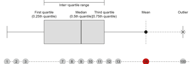
As quantiles are only sensitive to the ordering of the data but not to extreme values, they represent a robust alternative to the mean when evaluated at the center of a distribution. They can also offer a more informative summary of dispersion when the data are skewed or otherwise depart from normality. To illustrate these basic properties, consider for example in Figure 1 a set of values [1, 2, 3, 7, 8, 9, 10, 11, 12, 13, 100] arranged in ascending order. This set is clearly not normally distributed, but right-skewed in the sense that most observations are concentrated at lower values, with a long right tail. The 0.25th quantile, or equivalently the first quartile, of the set is the value below which there are at least 25% of cases, and in this example falls between 3 and 7 under common sample definitions. In the same vein, we can calculate the 0.75th quantile (third quartile), which is located between 11 and 12. Due to the existence of an extreme value (100) in this example, it is also apparent that compared to the mean 16, the median 9 is a more informative summary of the central location. These values can then be used to quantify the dispersion of the sample. Compared to the dispersion calculated by the sample standard deviation (approximately 28), which is more than twice the difference between the smallest and the second largest value of the sample, the interquartile range measured by the difference between the 0.25th and 0.75th quantile, as shown by the box plot in Figure 1, represents a more meaningful summary of the dispersion of the sample. Moreover, we can calculate another robust alternative to the mean-based standard deviation – the median absolute deviation (MAD), which is defined as the median of the absolute deviations from the median of the sample
 :
:
Sample quantiles and box-plot
 (1.1)
(1.1)
The MAD of the previous sample is 3, representing a more representative summary statistic for variability of the sample than the standard deviation.
As the figure also illustrates, the standard box-plots use quantiles to summarize the central tendency, dispersion, and skewness of a dataset, while also helping identify outliers. More generally, denote the value at
 th quantile as
 . For any
 , the inter-quantile range between the lower (
 ) and the upper (
 ) quantile can be computed as follows:
 (1.2)
(1.2)
which denotes the dispersion of the middle
 % of the sample.
Because of their robustness and their ability to characterize different parts of a sample or distribution, quantiles have become common statistics in descriptive summaries, quantification of uncertainty, and hypothesis testing in empirical research. A familiar example is the quantile-to-quantile (QQ) plot, which is commonly used to assess whether an empirical distribution is approximately normal. By comparing the quantiles of the dataset with the theoretical quantiles of a normal distribution, the QQ plot provides a simple visual diagnostic of deviations from normality.
1.4 Cumulative Distribution Function and Quantile Function
The cumulative distribution is closely related to the concept of quantiles. To understand quantiles more formally, it is thus helpful to clarify the relation between the cumulative distribution function and the quantile function. For any random variable
 , the cumulative distribution function evaluated at
 is defined as the probability that
 is less than or equal to
 :
:
 (1.3)
(1.3)
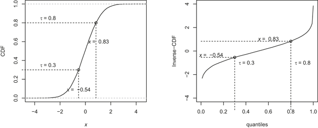
Statistically, scholars may be interested in knowing the location of a specific value within a distribution besides the mean. Consider the cumulative distribution function of the standard normal distribution as shown in Figure 2a. We might wish to know, for example, what proportion of the distribution lies below the values
 0.53 and 0.84. To do so, we trace each value on the horizontal axis up to the CDF and then across to the vertical axis. The resulting values are approximately 0.3 and 0.8, respectively (Figure 2a). In other words,
 0.53 corresponds to the 0.3th quantile and 0.84 to the 0.8th quantile of the standard normal distribution. The quantile function, as shown in Figure 2b, reverses this mapping by returning the value associated with a given cumulative probability.
Cumulative distribution function (a) and quantile function (b)
Formally, the
 th quantile function of a random variable
 , denoted
 , is defined as the generalized inverse of its cumulative distribution function:
 (1.4)
(1.4)
The quantile function is useful because it allows us to recover values associated with specified probability levels. This is central to many tasks in statistical analysis, including the construction of critical values, confidence intervals, prediction intervals, and other forms of uncertainty assessment.
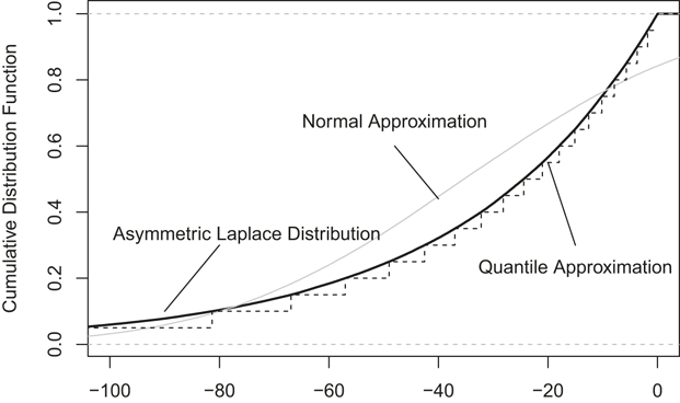
Although symmetrical distributions such as a normal distribution can often be summarized reasonably well by its central tendency and dispersion, that is, its mean and variance, the mean-based statistics become less informative when the distribution is asymmetric. Consider for instance a right-skewed distribution whose cumulative distribution function is plotted in Figure 3.Footnote 3 Approximating the distribution using a normal distribution with the corresponding mean and standard deviation will misrepresent the distribution around the median and in the tails. On the contrary, quantile approximation uses piece-wise information from the random sample, which, as shown by the dashed lines in the figure, yields a much better fit.
Approximation of a right-skewed distribution (asymmetric Laplace distribution with location parameter
 , scale parameter
 , and skewness parameter
 )
)
The substantive value of quantile-based summaries becomes especially clear when political outcomes are distributed unevenly across units. Take the distribution of ethnic voting in Bosnia as an example. Figure 4 illustrates the distribution using the violin plot. Based on data collected by Hadzic, Carlson, and Tavits (Reference Hadzic, Carlson and Tavits2020), the average municipal-level vote share of ethnic parties in national legislative elections is 80.99% (see Figure 4(a)). Compared to the median share of 84.89% (see Figure 4(b)), the mean value is a reduction of 4 percentage points. This indicates that the whole sample is distributed asymmetrically, with observations concentrated at relatively high vote shares and a longer tail toward lower values. In addition to the skewness, the spread of the distribution is wide, with the smallest share of 19.33% and the largest share of 99.49%.
Summary of the distribution of ethnic vote shares by mean (a) and quantile (b)
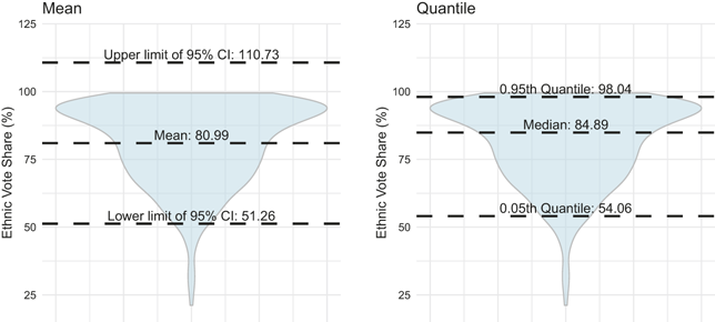
Moreover, as the left panel of the figure shows, if we use the 95% interval based on the normality assumption to quantify the spread of the variable, the upper limit of the 95% interval will exceed even the highest value of the sample, while the lower limit will underestimate the lowest values. Furthermore, because the quantification of the spread is symmetric around the mean, the mean-based approach is unable to reveal the skewness of the variable. In contrast, by examining the 0.95th and 0.05th quantile as illustrated in the right panel of Figure 4, we can find a sharp distinction between the upper and lower halves of the distribution: While there is only a 13.15% difference between the 0.95th quantile and the median, the difference between the median and the 0.05th quantile is 30.83%, more than twice the difference in the upper half. A focus on averages alone would therefore obscure substantively important variation across municipalities in the distribution of ethnic voting.
1.5 Conditional Quantiles
The illustrations in Section 1.4 show that quantiles provide added value to the mean by offering a more complete summary of a distribution. However, in political research, the central interest rarely lies in the distribution of a single variable alone. Instead, we want to investigate the effect of variables on the outcome of interest, that is, how changes in explanatory variables are associated with changes in the outcome. To reveal the conditional relationship between variables, we need to compute conditional quantiles. Conditional quantiles are “conditional” in the sense that the estimates depend on the covariates on the right-hand side of the estimation equation, and thereby they reveal local effects of a variable on the response across the whole distribution.
To show the benefits of using conditional quantiles, recall the standard linear model:
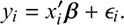 (1.5)
(1.5)
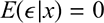
If we assume that the conditional expectation of the error term equals zero (i.e.,
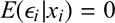 ), we obtain the conditional mean model. Subsequently, we can reformulate the equation with the response variable
 on the left-hand side and a vector of explanatory variables
 on the right-hand side (Lewis-Beck & Lewis-Beck, Reference Lewis-Beck and Lewis-Beck2015):
 (1.6)
(1.6)
This formulation summarizes the relationship between
 and
and
 at the conditional mean of the outcome. As a consequence, the covariate effect is represented by a single coefficient vector
 , rather than being allowed to vary across different parts of the conditional distribution. The coefficients can then be estimated by solving:Footnote 4
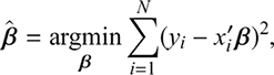 (1.7)
(1.7)
the familiar least-squares problem. While highly useful, the conditional mean neglects important information about potentially heterogeneous effects of
 on
on
 .
.
On the contrary, if we introduce an alternative formula
 (1.8)
(1.8)
by replacing the expectation
 with conditional quantiles
 , we are in a more flexible modeling situation. In this formula, each coefficient vector
 represents conditional effects at a specific quantile location
 of the response variable (for a formal proof, see e.g. Ding (Reference Ding2025, 294–297)). For
 , this becomes the conditional median model, which can be estimated by minimizing the sum of the absolute deviations:
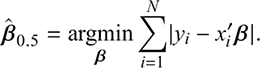 (1.9)
(1.9)
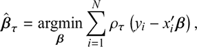
More generally, quantile regression estimates
 by minimizing the asymmetric absolute loss:
 (1.10)
where
 (for details of derivation, see Section 2.2). This objective function, often called the check function, gives asymmetric weights to positive and negative residuals and thereby identifies the conditional quantile.
Formally, the conditional quantile value of
 given
given
 can be written as
 (1.11)
where
 is the conditional cumulative distribution function. For each quantile level
 , we are able to get a quantile-specific effect
 that may differ from the average effect.
To interpret
 , we can regard it as the marginal change in the
 th quantile of the response variable due to a marginal change of the explanatory variable(s). In causal applications, and under additional identification assumptions, related quantile-based parameters can also be interpreted in terms of treatment effects at different points of the outcome distribution (Frandsen, Frölich, & Melly, Reference Frölich and Melly2010; Frölich & Melly, Reference Frandsen, Frölich and Melly2012), the details of which will be discussed in the subsection on quantile treatment effects in Section 5.
To illustrate the contrast between conditional means and conditional quantiles, return to the aforementioned example of ethnic voting. Suppose we are interested in the effect of wartime violence on ethnic voting, measured by wartime casualties and ethnic vote share, respectively (Hadzic, Carlson, & Tavits, Reference Hadzic, Carlson and Tavits2020). In a simple bivariate specification, the conditional mean can be calculated using the OLS regressing (logged) casualty against ethnic vote share. As illustrated by the solid line and the associated 95% confidence interval in Figure 5, the estimated mean relationship is not statistically distinguishable from zero. Once we examine the relationship across quantiles, however, a more differentiated pattern emerges. As shown by the fitted lines at the 0.05th, 0.5th, and 0.95th conditional quantiles in the figure, the positive relation between wartime violence and ethnic voting is strongest in lower quantiles of ethnic vote distribution and weakens as one moves toward the upper quantiles. This points to substantively meaningful heterogeneity across municipalities, possibly reflecting differences in prior levels or traditions of ethnic voting. Examining conditional quantiles alongside the conditional mean thus provides a fuller and more nuanced account of the relationship between wartime violence and ethnic voting.
Effects of wartime violence on ethnic voting
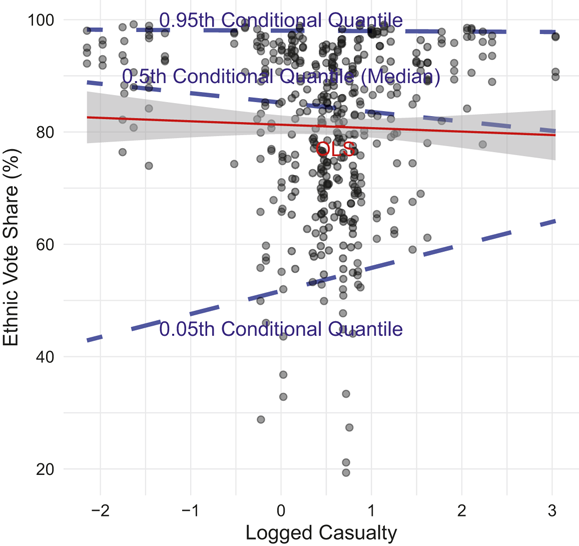
Note that for illustrative purposes, the depicted effects at this stage are solely based on the bivariate analysis, which consequently neglects potential confounding variables. In the following section, we will return to this example with a more complete analysis controlling for potential confounders.
1.6 Summary
This section has introduced the basic features of quantiles, the role of quantile functions, and the logic of conditional quantiles. According to the above illustrations, Table 1 summarizes the main differences between the mean-based and the quantile approach.
Mean-based approach

| Quantile approach

| |
|---|---|---|
| Central tendency | Mean | Median |
| Data distribution | Normality assumption | Without normality assumption |
| Error term |
|

|
| Spread | Standard deviation | Median absolute deviation |
| Estimated effect | Single average effect | Multiple local effects across quantiles |
| Estimation | Least squares | (Weighted) Least absolute deviation |
The quantile approach can be used to achieve the same goal as the mean-based approach, that is, to represent the central tendency of a sample or distribution. Compared to the mean, the median is more robust to extreme values. While the mean-based approach is often most straightforward under assumptions such as symmetry, homoscedasticity, or normally distributed errors, the quantile approach allows for more flexible distributions and relaxes the conditional-zero-mean assumption of the error term. When data contain heterogeneous units or the distribution of interest is skewed and asymmetric, quantiles provide additional information that would be overlooked when using the mean-based approach.
Mean-based approaches often summarize dispersion with the standard deviation and typically rely on variance-based measures for statistical inference. Without appropriate adjustments, this will lead to biased estimates of standard errors in the presence of heteroscedasticity, that is, when the variance of the error term is not constant. The quantile approach overcomes this problem by estimating local effects at different quantiles. The power of quantiles is not only about the complete description of data or distributions, but also the ability to investigate conditional relations between variables. This is particularly useful when we want to know how changes of the explanatory variables affect the outcome across its entire distribution. Therefore, in addition to robustness checks, quantile models allow researchers to examine distributional effects among heterogeneous political units, which will provide a more complete picture of the relationship between variables of interest.
This does not mean that quantile methods replace mean-based analysis in all applications. Rather, they complement it by expanding the range of questions that can be asked and answered empirically. Building on these foundations, the sections that follow extend the discussion to multivariate settings and show how quantile methods can be applied to a variety of statistical and substantive problems in political science.
2 Quantile Models for Continuous Responses
2.1 Introduction
This section introduces the classical quantile model, which focuses on continuous response variables. In contrast to the univariate setting discussed in the previous section, it demonstrates how to estimate conditional quantiles for the continuous response variable in multivariate settings. In continuous scales, the response variable is represented by values on the real number line, providing rich information commonly seen in empirical political research. Variables of this kind, such as vote shares, party size, and level of turnout, carry substantive meanings through differences in magnitude. Modeling continuous response variables usually eliminates the need for additional data transformations that are common for evaluating discrete response variables discussed in the following chapters. Consequently, the coefficients obtained from quantile models directly reflect how the response variable changes when the explanatory variables shift by one unit at the specified quantile location.
Formally, adopting linear parameterization, quantile regression models the data with the continuous response variable
 at
at
 th quantile as
 (2.1)
(2.1)
where
 corresponds to the variables of the data, and
 is a vector of coefficients associated with the variables at quantile
 . The core task of quantile regression is to estimate values of
 given
given
 and
and
 , the details of which will be discussed in the following subsection.
2.2 Estimation and Inference in Quantile Regression
In contrast to the conditional mean-based approach that minimizes a squared loss function, the conditional
 th quantile as a solution to the above equation is obtained by minimizing an asymmetric loss function
 , where each component is weighted either by
 or
or
 (Yu & Moyeed, Reference Yu and Moyeed2001):
 (2.2)
(2.2)
In this formula,
 is a cumulative distribution function, and
 represents the value of the
 th quantile as calculated by Equation (1.4). According to Equation (2.2), the quantile loss function uses all the sample information, instead of splitting the sample, to derive the quantile values. Because the linear loss function depends not on certain covariate values but on covariate orderings, the quantile estimators are more robust than the least squares estimators in the presence of extreme values.
By solving the first order condition, we have the
 th sample objective function evaluated at
 as
as
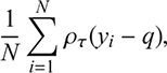 (2.3)
(2.3)
where
 (2.4)
(2.4)
is known as the check function and
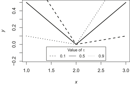
 denotes the indicator function. As illustrated in Figure 6, the check function takes different shapes when different quantiles are specified. The function is symmetric when evaluated at the median (0.5th quantile shown by the solid line).
Check functions at different quantiles
Given a linear model
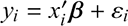 , the
, the
 th quantile regression estimator minimizes the above equation by replacing
 with
with
 . In the model, we commonly assume
 . If
. If
 , the model reduces to a median regression. The goal is to estimate the values of
 for each
 by solving the following minimization problem:
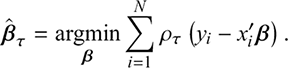 (2.5)
(2.5)
The common solution to this minimization problem is based on the technique of linear programming, which iterates through points and lines on a polyhedral surface to find the optimal estimates. The standard errors and confidence intervals are then calculated based on the asymptotic normality assumption or by repeated sampling using bootstrap methods (Davino, Furno, & Vistocco, Reference Davino, Furno and Vistocco2014; Koenker, Reference Koenker2005). It can be shown that under certain regularity conditions, the estimated quantile coefficients
 are asymptotically normal:
 (2.6)
(2.6)
where
 and
and
 is the conditional density of the error term evaluated at zero (Buchinsky, Reference Buchinsky1998).
Alternatively, recent developments in Bayesian methods allow researchers to estimate quantile regression using the Markov chain Monte Carlo (MCMC) sampling procedure (Yu & Moyeed, Reference Yu and Moyeed2001). This is done by imposing appropriate (or uninformative) priors on the parameters to be estimated, and then combining the prior with the likelihood function to form the posterior distribution, which can be subsequently sampled using MCMC algorithms. Compared to the frequentist approach which relies on asymptotic properties, the advantage of the Bayesian estimation is that it provides a natural quantification of estimation uncertainty from random draws of the posterior distribution.
As proved by Koenker and Bassett (Reference Koenker and Bassett1978, 39) (Theorem 3.2 of the paper), there are a number of desirable equivariance properties of the estimated coefficients
 that can be statistically interesting to applied researchers:
 (2.7)
(2.7)
 (2.8)
(2.8)
 (2.9)
(2.9)
 (2.10)
where the first two equations suggest that the coefficients are equivariant under scalar transformations of the response variable. This property is particularly useful for analyzing discrete response variables. The last two equations state that the coefficients are equivariant to a location shift of the response variable and reparameterization of the design matrix. Thus, it provides more flexibility for regression analysis.
To evaluate the goodness of fit of quantile regression, Koenker and Machado (Reference Koenker and Machado1999) also developed an analog of the
 -squared measure:
 (2.11)
where
 and
and
 . Here,
 and
and
 represent respectively the predicted response value and the sample quantile of the response variable without controlling for covariates.
For applied researchers, fortunately, there are statistical software packages that can perform estimation tasks for us. So here I will not delve into the specifics of the various types of estimators and their solution concepts. To demonstrate the utility of quantile estimation tools for analyzing continuous response variables, we can utilize two open-source software packages written in the R language. The first is the quantreg package developed by Roger Koenker and continuously enhanced by numerous statisticians (Koenker, Reference Koenker2025). It offers a diverse set of functions for estimating conditional quantiles using a frequentist approach. The second package, bayesQR, was created by Dries Benoit, Rahim Al-Hamzawi, Keming Yu, and Dirk Van den Poel (Benoit & Van den Poel, Reference Benoit and Van den Poel2017), primarily based on the methods proposed in Benoit and Van den Poel (Reference Benoit and Van den Poel2012) and Benoit, Alhamzawi, and Yu (Reference Benoit, Alhamzawi and Yu2013). This package is used for Bayesian quantile regression estimation. To install and load these packages, we can execute the following codes, which download the package sources from the Comprehensive R Archive Network (CRAN) to the local drive and load the packages into the current working environment.

Code 1.1
1 # Install two packages from CRAN repository
2 install.packages(c("quantreg", "bayesQR"))
3 # Load the packages
4 library(quantreg)
5 library(bayesQR)
In what follows, the quantile estimation will be illustrated using two real-world political examples of ethnic voting and political representation. For the estimation of the data, the analysis will mainly exploit the rq() function from the quantreg package (details on the quantreg package are preserved for the next section). Note that estimating the data of the two examples using the Bayesian approach without informative priors yields similar results.
2.3 Example of Ethnic Voting
To illustrate the quantile model, consider again the ethnic voting example studied by Hadzic, Carlson, and Tavits (Reference Hadzic, Carlson and Tavits2020). The authors argue that community-level experience with wartime violence increases the salience of ethnic identities, making it important for postwar vote choice. Employing a difference-in-differences design on a panel dataset from pre- and postwar elections of Bosnia, Hadzic, Carlson, and Tavits (Reference Hadzic, Carlson and Tavits2020) find strong support for a positive effect of wartime violence on postwar ethnic voting. Yet the theoretical logic of the argument also suggests that this effect may not be uniform across communities. Quantile regression provides a natural way to examine this possibility by asking whether the relationship between wartime violence and postwar ethnic voting differs across the lower and upper parts of the conditional outcome distribution. In this example, different conditional quantiles represent the varying proportions of postwar ethnic voting in different communities. For example, a conditional quantile of 0.1 would roughly represent the bottom 10% communities (about 10 communities in the sample) where the proportion of ethnic voting is lower than the rest 90% of the communities in the sample. Because communities with low proportions of ethnic voting in postwar elections are mostly those communities with low prewar ethnic voting, the quantile approach also allows us to examine the variation of ethnic voting via the lens of diverse cultures of cooperation and inter-ethnic relations in different communities.
In the literature on civil conflict, there are at least two competing theories explaining the impact of wartime violence on the politicization of ethnicity. One theory posits that fears of violence and prewar norms of cooperation will reduce politicization of ethnicity after the war (Bellows & Miguel, Reference Bellows and Miguel2009; Blattman, Reference Blattman2009; Gilligan, Pasquale, & Samii, Reference Gilligan, Pasquale and Samii2014; Voors et al., Reference Voors, Nillesen and Verwimp2012; Wood, Reference Wood2003). This could be attributed to the possibility of more altruistic individuals remaining disproportionately in war-plagued communities, or to the need of the remaining populace to collectively confront threats and psychological distress (Gilligan, Pasquale, & Samii, Reference Gilligan, Pasquale and Samii2014). Conversely, another theory emphasizes the heightened salience of ethnicity and the role of war-enhanced group identification in promoting postwar ethnic voting (Hadzic, Carlson, & Tavits, Reference Hadzic, Carlson and Tavits2020; Wilkinson, Reference Wilkinson2006).Footnote 5 According to this theory, ethnic violence during wartime amplifies rather than diminishes inter-ethnic distrust, rendering ethnic parties a more appealing avenue for post-war representation (Hadzic, Carlson, & Tavits, Reference Hadzic, Carlson and Tavits2020). However, the conflicting theories and their empirical evidence also indicate possible diversity among various subgroups of a population that may react differently to ethnic violence. For example, based on the level of prewar social cohesion, the influence of exposure to ethnic violence during wartime on ethnic voting may fluctuate across different communities. It is plausible to expect that in regions where social cohesion is high and thus ethnic polarization is low, the experience of wartime violence is likely to reduce ethnic voting after the war. However, in regions where there is relatively high ethnic polarization, we may expect a positive effect of wartime violence on ethnic voting. If such heterogeneity exists, revisiting the data with quantile regression could potentially unveil varying subgroup effects that have significant implications but have been largely disregarded in the literature.
The data collected by Hadzic, Carlson, and Tavits (Reference Hadzic, Carlson and Tavits2020) record election results in Bosnia both before and after the Bosnian Civil War fought between 1992 and 1995, which are publicly available.Footnote 6 After downloading the data, we can load and explore the detailed features of the variables with the following codes.
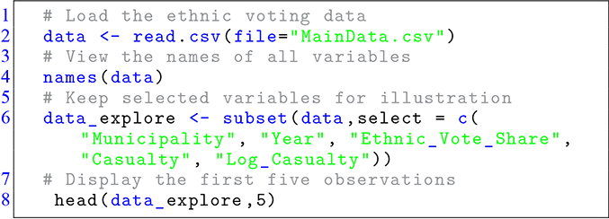
Code 1.2
1 # Load the ethnic voting data
2 data <- read.csv(file="MainData.csv")
3 # View the names of all variables
4 names(data)
5 # Keep selected variables for illustration
6 data_explore <- subset(data,select = c(
    "Municipality", "Year", "Ethnic_Vote_Share",
  "Casualty", "Log_Casualty"))
7 # Display the first five observations
8 head(data_explore,5)
As shown in Table 2, the response variable Ethnic_Vote_Share measures the municipal-level percentage of votes cast for ethnic parties and varies over time. More specifically, the data come from 107 Bosnian communities, including Velika Kladusa and Cazin in years 1990, 2006, 2010, and 2014. The casualty measure records the intensity of ethnic violence and is taken from the Bosnian Book of the Dead, which records the percentage of the total number of confirmed dead and missing against the prewar municipal population (Hadzic, Carlson, & Tavits, Reference Hadzic, Carlson and Tavits2020, 350). The variable Log_Casualty is the log-transformed value of Casualty. Using these measures, we are able to first explore the primary relation between (logged) casualty and ethnic vote share using scatter plots.
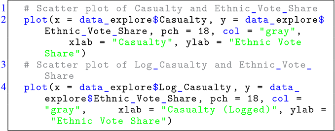
Code 1.3
1 # Scatter plot of Casualty and Ethnic_Vote_Share
2 plot(x = data_explore$Casualty, y = data_explore$
 # # #Ethnic_Vote_Share, pch = 18, col = "gray",
 # # #xlab = "Casualty", ylab = "Ethnic Vote
 # # #Share")
3  # # Scatter plot of Log_Casualty and Ethnic_Vote_Share
4 plot(x = data_explore$Log_Casualty, y = data_
 # # #explore$Ethnic_Vote_Share, pch = 18, col =
 # # #"gray",     xlab = "Casualty (Logged)", ylab =
 # # #"Ethnic Vote Share")
| Municipality | Year | Ethnic_Vote_Share | Casualty | Log_Casualty | |
|---|---|---|---|---|---|
| 1 | Velika Kladusa | 2006 | 21.15 | 2.05 | 0.72 |
| 2 | Velika Kladusa | 2010 | 19.33 | 2.05 | 0.72 |
| 3 | Velika Kladusa | 2014 | 33.37 | 2.05 | 0.72 |
| 4 | Cazin | 2006 | 64.84 | 1.47 | 0.38 |
| 5 | Cazin | 2010 | 61.95 | 1.47 | 0.38 |

|

|

|

|

|

|
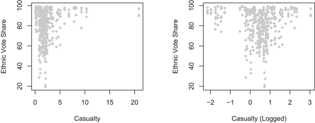
The scatter plots in Figure 7 reveal that the original measure of casualty is right-skewed (left panel), but is close to a normal distribution in the logarithmic scale (right panel). Therefore, as with Hadzic, Carlson, and Tavits (Reference Hadzic, Carlson and Tavits2020), the logged version of the casualty measure is adopted for the regression analysis. The quantreg package is used to estimate the conditional quantiles, with the parameter tau specifying the quantiles to be estimated. For the values of tau, a range of quantiles from 0.1 to 0.9 are specified. Here, lower quantiles may be interpreted as pertaining to communities where the proportion of ethnic voting is relatively low, and upper quantiles represent those communities where votes are more divided along ethnic lines. Given control variables, conditional quantiles can also be interpreted as capturing different positions in the distribution of ethnic vote share across communities, which may reflect varying degrees of ethnic political alignment. This allows us to ask whether the association between wartime violence and ethnic voting differs systematically across communities located at different points of the ethnic-voting distribution.
Scatter plots of correlation between casualty(a)/logged casualty (b) and ethnic vote share
For illustrating the quantile estimation of the effects of wartime violence on ethnic voting, let us first consider a simple model of the relation between the two variables. A more comprehensive model in the subsequent analysis will also take into account the spatial and temporal variation. Here, the rq function from the quantreg package is used (Koenker, Reference Koenker2025), and the computational codes are shown in the following. The results can be visualized and printed using the functions plot and summary.
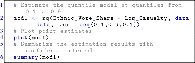
Code 1.4
1 # Estimate the quantile model at quantiles from 0.1 to 0.9
2 mod1 <- rq(Ethnic_Vote_Share ~ Log_Casualty, data = data, tau = seq(0.1,0.9,0.1))
3 # Plot point estimates
4 plot(mod1)
5 # Summarize the estimation results with confidence intervals
6 summary(mod1)
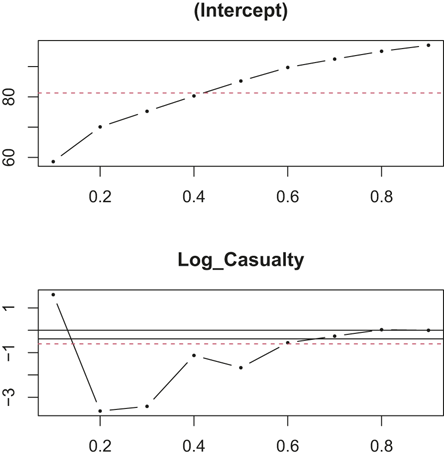
Figure 8 shows the point estimates of the effects for the intercept and casualty at different quantiles, where the dashed horizontal lines represent the OLS estimates. In both panels of the figure, the x-axis represents different quantile levels, and the y-axis shows the estimated effects of a variable at different quantiles, with the dotted line indicating how the effects change with increasing quantile levels. Compared to a single average effect estimated by the OLS, the U-shaped quantile estimation curve of casualty in the lower panel demonstrates that the effects of casualty on ethnic voting may differ across subgroups. In the lower quantiles less than 0.6 (except for 0.1), the effects are negative, while in the upper quantiles higher than 0.6, the effects become positive. These results reveal significant differences in the effects of casualty on ethnic voting between communities with diverse levels of ethnic voting in wartime. Because quantiles are measured on shares of ethnic votes (and thus ethnic polarization) across communities, it indicates that exposure to violence may affect ethnic voting differently depending on the ethnic polarization in each community. In particular, in lower quantiles where ethnic polarization is relatively low, the effects of wartime violence (Log_Casualty) on ethnic voting become negative, which suggests that in communities with low ethnic polarization, exposure to ethnic violence is likely to increase inter-ethnic trust and postwar social cohesion (and thus reduces the proportion of ethnic voting). This is the case for Bosnian communities such as Centar Sarajevo, Novo Sarajevo, Srebrenik, Tuzla, and Velika Kladusa, where the average proportion of ethnic voting is lower than the 0.1th quantile of the whole sample (i.e., 65% ethnic vote share). However, as demonstrated by the positive effects in the upper quantiles, the opposite is true in other communities where ethnic polarization is high. Overall, the results show that in lower quantile regions where the proportion of ethnic voting is relatively low, the OLS is likely to overestimate the effect of casualty, while in upper quantiles it is more likely to underestimate the effect.
Point estimates of quantile effects for ethnic voting example
The simple bivariate model is useful for illustration, but it leaves open the possibility that the estimated pattern is confounded by differences across years and municipalities. To better account for potential confounding factors, we now examine a more comprehensive model that takes into account the spatial and temporal variation. More specifically, we follow the model specification and the difference-in-differences (DID) design of Hadzic, Carlson, and Tavits (Reference Hadzic, Carlson and Tavits2020), with dummy controls of years before and after the civil war. The analysis also includes the fixed effects of regions. The following codes show the details of the quantile estimation procedure for the ethnic voting data.
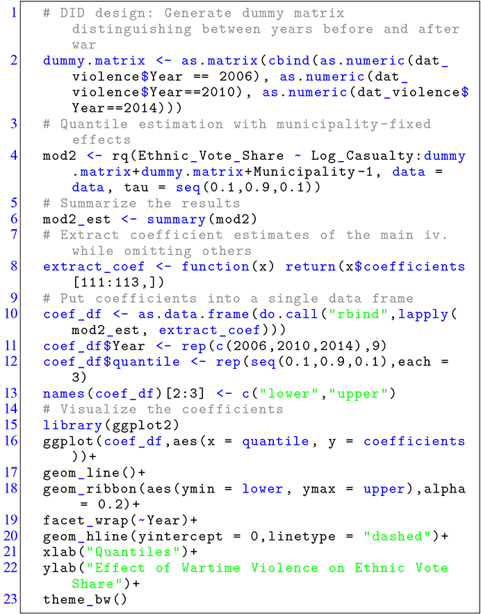
Code 1.5
1 # DID design: Generate dummy matrix distinguishing between years before and after war
2 dummy.matrix <- as.matrix(cbind(as.numeric(dat_violence$Year == 2006), as.numeric(dat_violence$Year==2010), as.numeric(dat_violence$Year==2014)))
3 # Quantile estimation with municipality-fixed effects
4 mod2 <- rq(Ethnic_Vote_Share ~ Log_Casualty:dummy.matrix+dummy.matrix+Municipality-1, data = data, tau = seq(0.1,0.9,0.1))
5 # Summarize the results
6 mod2_est <- summary(mod2)
7 # Extract coefficient estimates of the main iv. while omitting others
8 extract_coef <- function(x) return(x$coefficients[111:113,])
9 # Put coefficients into a single data frame
10 coef_df <- as.data.frame(do.call("rbind",lapply(mod2_est, extract_coef)))
11 coef_df$Year <- rep(c(2006,2010,2014),9)
12 coef_df$quantile <- rep(seq(0.1,0.9,0.1),each = 3)
13 names(coef_df)[2:3] <- c("lower","upper")
14 # Visualize the coefficients
15 library(ggplot2)
16 ggplot(coef_df,aes(x = quantile, y = coefficients))+
17 geom_line()+
18 geom_ribbon(aes(ymin = lower, ymax = upper),alpha = 0.2)+
19 facet_wrap(~Year)+
20 geom_hline(yintercept = 0,linetype = "dashed")+
21 xlab("Quantiles")+
22 ylab("Effect of Wartime Violence on Ethnic Vote Share")+
23 theme_bw()
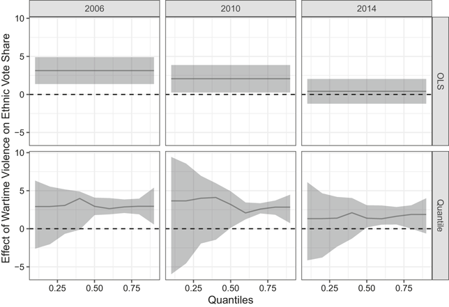
The results of the coefficient estimates of the OLS and quantile regression are displayed in Figure 9, which shows the results in 2006 (a – left panel), 2010 (b – middle panel), and 2014 (c – right panel) in comparison to the baseline year 1990 in the prewar period. The OLS estimation follows Model 1 in table 1 of Hadzic, Carlson, and Tavits (Reference Hadzic, Carlson and Tavits2020, 353) with clustered (on municipality and year) robust standard errors. Compared to the average positive estimates by the OLS, all three panels of the figure show that while the positive effects of wartime violence on ethnic voting are evident in the upper quantiles where ethnic voting is more common, the effects are insignificant in the lower quantiles (quantiles lower than 0.5). Compared to the results in 2006 and 2010, the reduced effect of wartime violence on ethnic voting in the middle and upper quantiles in 2014 also indicates that the impact of wartime memory of ethnic violence seems to be decreasing at the community level.
Estimated effects of wartime violence on ethnic vote share over postwar years and across quantiles
Given that communities with low proportions of ethnic voting in postwar elections are mostly those communities with low prewar ethnic voting, it is plausible to associate the level of ethnic voting with the culture of cooperation and inter-ethnic relations in different communities. For example, as shown in Table 3, for communities such as Centar Sarajevo, Novo Sarajevo, Srebrenik, and Tuzla, where wartime violence has no discernible effects, they are all below the 0.1th quantile (i.e., around 65%) measured by the proportion of ethnic voting in both pre- and postwar periods.Footnote 7 And except for Srebrenik, the rest of these communities have lower prewar ethnic concentration measured by Herfindahl–Hirschman indices compared to the average of the sample (Hadzic, Carlson, & Tavits, Reference Hadzic, Carlson and Tavits2020). This implies that in regions without a long-standing tradition of ethnic voting, the mechanism by which wartime violence affects ethnic voting may be different. In areas with a strong culture of cooperation and mild ethnic divisions, it may be easier to return to this norm after the ethnic conflict without a heightened risk of ethnic polarization. This process is less likely or much slower in regions where the culture of cooperation is absent.
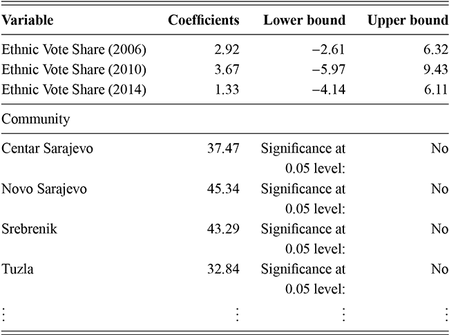
Table 3 Long description
The table shows quantile regression results at the 0.1th quantile for ethnic vote share and community fixed effects in Bosnian municipalities. The first section lists coefficients for ethnic vote share in 2006 (2.92), 2010 (3.67), and 2014 (1.33), with 95% confidence intervals spanning -2.61 to 6.32, -5.97 to 9.43, and -4.14 to 6.11, respectively. The second section presents fixed-effects for selected communities: Centar Sarajevo (37.47), Novo Sarajevo (45.34), Srebrenik (43.29), and Tuzla (32.84). None of these fixed-effects are significant at the 5% level. Additional communities are included in the model but omitted here. These results highlight that communities with low prewar ethnic voting remain at the low end of the ethnic vote distribution postwar, suggesting a persistent culture of inter-ethnic cooperation.
Note: Fixed-effects of other communities omitted here. The upper and lower bounds correspond to the 95% confidence interval.
These empirical findings from estimating the quantile model help to reconcile the two competing theories of the effect of wartime violence on ethnic voting. This suggests that the concrete effect of violence may be dependent on the prior inter-ethnic relations in different communities. Thus, even this simple replication study using quantile models opens up interesting possibilities for further research, which could delve deeper into the local effects that explain the variation of ethnic voting between different regions.
2.4 Example of Political Representation
As another example, political representation by parties is usually not about reflecting average societal preferences. Parties tend to have closer ties to certain societal groups, and more conflictual relations with others. Because these relations can be disrupted or enhanced by external threats, Weschle (Reference Weschle2019) argues that economic crises impact the way parties represent the society, which further depends on whether the parties have cooperative or conflictual relations with different societal groups. Under external threats, political parties need not only to be responsive to their own constituencies, but also be responsible to other societal groups in order to unite the whole nation to better cope with the threats (Bueno de Mesquita, Reference Bueno de Mesquita1981; Chowanietz, Reference Chowanietz2011; Indridason, Reference Indridason2008; Lijphart, Reference Lijphart1996). This consequently leads to changes in the parties’ societal relations with the groups they are closest to and least close to. More specifically, parties have to trade-off between representing the interests of their own constituencies faithfully and being responsive to other societal groups for a collective effort in handling external threats. Therefore, in times of crises, we would expect empirically that parties’ relations with the societal group they are closest to become less cooperative, while their relations with the groups they are least close to become less conflictual (Weschle, Reference Weschle2019). However, these heterogeneous relations are difficult to investigate using the traditional mean-based models, which merely reveal a single average effect.
To investigate the influence of economic crises on the political representation of diverse societal groups, Weschle (Reference Weschle2019) developed a latent network model, which draws inferences about the relationship between political parties and societal groups. Subsequently, he utilized quantile models to analyze the effects of economic crises on parties’ relationships with different types of societal groups. The latent network model allows for identifying parties’ societal relations by estimating the cooperation scores, which measure the level of cooperation or conflict between a party and a societal group for eleven eurozone countries between 2001 and 2011. Using this measure as the dependent variable, the quantile models estimate varying effects of economic crises on political representation, with different quantiles capturing different parts of the latent cooperation-score distribution. More specifically, higher quantiles in the model indicate the societal groups with which parties have better initial relations, while lower quantiles focus on those groups that have a less cooperative relationship with the parties.
To demonstrate how quantile models improve our substantive understanding of political representation in times of crises, we replicate the analysis of Weschle (Reference Weschle2019). The following codes load the data and draw quantile fitting lines against a scatter plot. Here, the variable coopscore_1 represents a random draw of the cooperation scores from the latent network model of political representation, and GDP growth per capita is used to examine the impact of economic crises.Footnote 8
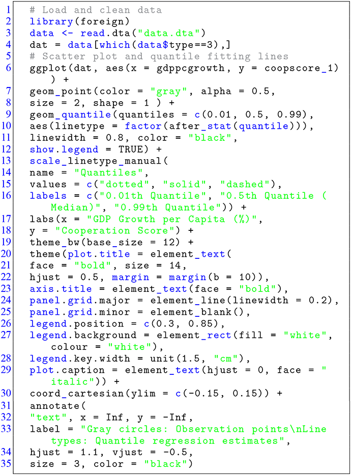
Code 1.6
1 # Load and clean data
2 library(foreign)
3 data <- read.dta("data.dta")
4 dat = data[which(data$type==3),]
5 # Scatter plot and quantile fitting lines
6 ggplot(dat, aes(x = gdppcgrowth, y = coopscore_1)) +
7 geom_point(color = "gray", alpha = 0.5,
8 size = 2, shape = 1 ) +
9 geom_quantile(quantiles = c(0.01, 0.5, 0.99),
10 aes(linetype = factor(after_stat(quantile))),
11 linewidth = 0.8, color = "black",
12 show.legend = TRUE) +
13 scale_linetype_manual(
14 name = "Quantiles",
15 values = c("dotted", "solid", "dashed"),
16 labels = c("0.01th Quantile", "0.5th Quantile (Median)", "0.99th Quantile")) +
17 labs(x = "GDP Growth per Capita (%)",
18 y = "Cooperation Score") +
19 theme_bw(base_size = 12) +
20 theme(plot.title = element_text(
21 face = "bold", size = 14,
22 hjust = 0.5, margin = margin(b = 10)),
23 axis.title = element_text(face = "bold"),
24 panel.grid.major = element_line(linewidth = 0.2),
25 panel.grid.minor = element_blank(),
26 legend.position = c(0.3, 0.85),
27 legend.background = element_rect(fill = "white", colour = "white"),
28 legend.key.width = unit(1.5, "cm"),
29 plot.caption = element_text(hjust = 0, face = "italic")) +
30 coord_cartesian(ylim = c(-0.15, 0.15)) +
31 annotate(
32 "text", x = Inf, y = -Inf,
33 label = "Gray circles: Observation points\nLine types: Quantile regression estimates",
34 hjust = 1.1, vjust = -0.5,
35 size = 3, color = "black")
Figure 10 shows the three quantile fitting lines in the 0.01th, 0.5th, and 0.99th quantiles that are superimposed onto the scatter plot between GDP growth per capita and cooperation scores. The upper quantile (0.99th quantile) represents societal groups with which a party has a cooperative relationship, while the lower quantile (0.01th quantile) represents those with which a party has a conflictual relationship. The median (0.5th quantile), in contrast, represents groups with which a party has neither a close nor conflictual relation.
Scatter plot of GDP growth per capita and cooperation scores between political parties and societal groups
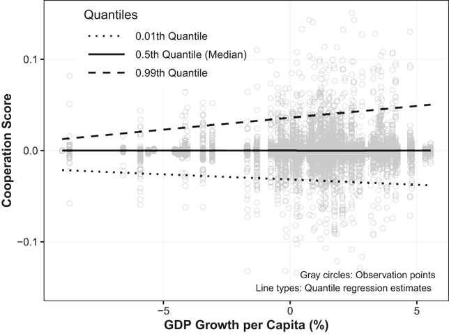
According to the fitted quantile lines in Figure 10, there is no discernible effect at the median, but the opposing effects at the lower and upper quantiles of 0.01 and 0.99 are visible. This suggests that the impact of the economic crisis on the relation between a party and a societal group may vary depending on the initial relationship between them. Specifically, as the economy expands, it will enhance parties’ cooperative relations with societal groups they are most aligned with (dashed line of the 0.99th quantile), whereas economic crises will damage these relationships, resulting in reduced cooperation. Conversely, as indicated by the dotted fitting line for the 0.01th quantile, during crises, parties endeavor to improve their relations with societal groups they originally have conflictual relations with. These results from the quantile models suggest that economic crises tend to disrupt representation and motivate politicians and parties to “put politics aside” by cooperating more with previously distant groups (Weschle, Reference Weschle2019). If researchers were to rely solely on mean-based models, these new theoretical and empirical perspectives would likely have gone uninvestigated.
Note that the above analysis simply examines the relation between the main explanatory variable and the response variable. To account for potential confounding variables, the next step is to include them in the full model specification. Weschle’s (Reference Weschle2019) study includes control variables such as trade openness, population, election year, number of parties, number of events in political communication, and mean cooperation scores for each country and year, which are also included in this replication analysis. To demonstrate the varying effects of economic conditions on political representation, we can specify the lower (0.25th), middle (0.5th), and upper (0.75th) quantiles and estimate the respective conditional quantile effects.Footnote 9 Using the first random draw of cooperation scores, the following codes complete the task and summarize the estimation results for each quantile. Note that compared to the original analysis, the response variable is rescaled by a factor of 1,000 to make the estimates more interpretable.
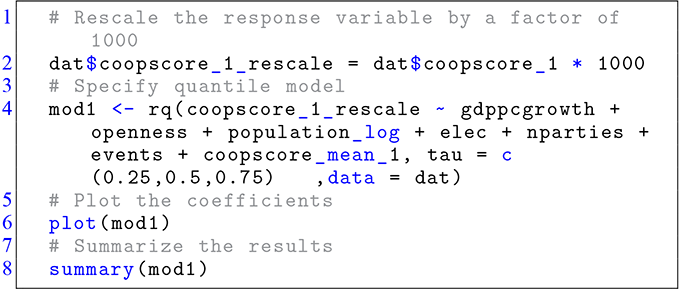
Code 1.7
1 # Rescale the response variable by a factor of 1000
2 dat$coopscore_1_rescale = dat$coopscore_1 * 1000
3 # Specify quantile model
4 mod1 <- rq(coopscore_1_rescale ~ gdppcgrowth + openness + population_log + elec + nparties + events + coopscore_mean_1, tau = c(0.25,0.5,0.75)   ,data = dat)
5 # Plot the coefficients
6 plot(mod1)
7 # Summarize the results
4 summary(mod1)
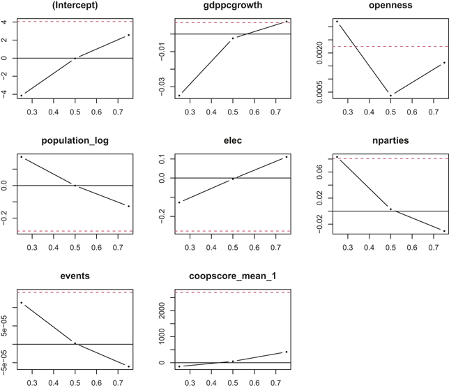
Figure 11 demonstrates that the quantile model reveals considerable variation of the effects of different covariates across quantiles compared to the OLS estimates shown by the dashed horizontal lines. For all the control variables, including the intercept, the estimated coefficients have opposite directions between the lower and upper quantiles. The large discrepancy between estimates of the OLS and median regression (quantile model evaluated at 0.5th quantile) also suggests that the heterogeneity in the data cannot be well accounted for by the mean-based model.Footnote 10
Coefficient estimates at three conditional quantiles (0.25th, 0.5th, and 0.75th) for political representation example
Note: Black dotted lines represent quantile estimates and horizontal dashed lines represent OLS estimates.
In addition to the average estimates by the OLS, the results of Table 4 indicate that the effect of GDP growth per capita on political representation varies across quantiles. In the lower quantile (0.25th quantile) of the response variable, the effect is significantly negative, while in the upper quantile (0.75th quantile) the effect is significantly positive. Although the median estimate is statistically distinguishable from zero, its magnitude is substantively very small. This suggests that on average economic conditions have little effect on political representation, but when the economy is doing well, parties are more likely to represent their core constituents. Conversely, when the economy is doing poorly, parties appear to move toward less conflictual relations with groups with which they originally conflict. Thus, this finding indicates that in times of economic crisis, political parties must navigate a distinct balance between catering to their own constituencies and addressing the interests of diverse societal groups to foster national unity. Compared to normal times, the relation between political parties and the societal groups they are least close to becomes less conflictual during periods of crisis. This is the kind of heterogeneous adjustment that a mean-based model is poorly equipped to detect.
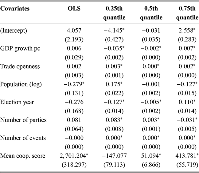
Table 4 Long description
The table presents O L S and quantile regression results (0.25th, 0.5th, 0.75th quantiles) for a political representation outcome. Covariates include intercept, G D P growth per capita, trade openness, population (log), election year, number of parties, number of events, and mean cooperation score. Coefficients show substantial variation across quantiles: G D P growth is significantly negative at the 0.25th quantile, near zero at the median, and positive at the 0.75th quantile. Trade openness and population effects also vary by quantile. Mean cooperation score is strongly positive in O L S and upper quantiles. Asterisks indicate 95% significance. These results highlight that economic and structural factors affect political representation differently across the distribution, reflecting heterogeneous party responsiveness under different economic conditions.
The asterisk * denotes significance at 95% confidence level.
Standard errors are shown in parentheses.
As also shown in the table, the coefficients of the rest of the variables, such as population, election year, number of parties, and mean cooperation score, are significantly different between lower and upper quantiles.Footnote 11 These results are important for understanding democratic representation in times of crisis, which would remain unknown without exploring the quantile behavior of the explanatory variables over the distribution of the response variable.
To eliminate concerns about potential heterogeneity across countries and over years, we may also control for the country- and/or year-fixed effects. For simplicity, the example presented here uses a single draw of cooperation scores as the response variable. Yet the example is sufficient to demonstrate the substantive payoff of quantile analysis. To have a more complete analysis, more observations can be easily included from the data of Weschle (Reference Weschle2019), which will generate similar results.
2.5 Summary
The discussion in this section has shown that, although mean-based models remain central to empirical analysis, they are not always well suited to questions involving substantial heterogeneity. Concentrating on the means has prevented researchers from using more suitable techniques for analyzing heterogeneous political phenomena. For many political studies, the quantile approach allows for the evaluation of heterogeneous data that cannot be satisfactorily analyzed by mean-based models. It not only provides comprehensive summary statistics for the location and spread of a given sample, but also reveals a more detailed relationship between the dependent and explanatory variables. The utility of quantile models is not limited to examining heterogeneous data. Even when the primary interest is not heterogeneity itself, quantile models can still serve as a valuable diagnostic by revealing whether empirical relationships are stable across the distribution.
Using the examples of ethnic voting and political representation, this section illustrates the utility of the quantile approach for applied political research examining continuous response variables in multivariate settings. It shows how quantile models can be beneficial for exploring heterogeneous political units and identifying varying effects across the distribution of the outcomes. The new results have unveiled intriguing insights that were previously undisclosed by the traditional mean-based models.
For instance, in the case of the ethnic voting example, contrary to the average finding indicating a singular positive effect of wartime violence on postwar ethnic voting, the results based on the quantile model demonstrate that the effect is contingent on the degree of prewar ethnic polarization. In communities where there is a strong prewar norm of inter-ethnic cooperation, it is much easier to return to the norm without an increased risk of postwar ethnic polarization. Conversely, in communities with historically high ethnic divisions, the memory of conflict may instead intensify ethnic polarization. Revisiting the example of political representation also reveals heterogeneous effects of economic crises on political representation of parties with different societal groups. While economic conditions have little impact on political representation on average, parties tend to be more responsive to groups with which they originally conflict when the economy falters. These findings provide crucial insights that would otherwise remain unknown.
Overall, these examples highlight the broader contribution of quantile models to political analysis. They allow researchers to move beyond average effects, to detect substantively meaningful heterogeneity, and to generate more thorough interpretations of political processes. The sections that follow build on this foundation by extending the quantile framework to additional outcome types and modeling settings.
3 Quantile Models for Binary Choices
3.1 Introduction
Besides the continuous response variables introduced in the previous section, many important political outcomes take the form of discrete choices. Such outcomes are central to the study of vote choice, partisan identification, government formation, legislative policymaking, and many other political decisions. For example, researchers might be interested in exploring how conflict among coalition parties affects the adoption of bills with inherently different success rates, or how ideological factors impact coalition formation among coalitions with varying likelihoods of entering government. However, despite the advances in modeling discrete choice data in political science (see, e.g., Alvarez & Glasgow, Reference Alvarez and Glasgow1999; Beck, Katz, & Tucker, Reference Beck, Katz and Tucker1998; Carter & Signorino, Reference Carter and Signorino2010; Glasgow, Reference Glasgow2011, Reference Glasgow2022; McGrath, Reference McGrath2015; Poole, Reference Poole2000; Rainey, Reference Rainey2016; Sartori, Reference Sartori2003; Traunmüller, Murr, & Gill, Reference Traunmüller, Murr and Gill2015), existing estimators are typically centered on conditional means or choice probabilities and pay less attention to distributional heterogeneity. This can lead to incomplete or even inaccurate inferences when heterogeneity among individuals or subgroups of a population is averaged out in the estimation process of discrete response variables.
Because quantiles have useful equivariance properties under monotonic transformations (Koenker & Machado, Reference Koenker and Machado1999), they are well suited for modeling discrete choice data which usually require in estimation a certain form of nonlinear transformation (Horowitz, Reference Horowitz1992). As with quantile estimation of continuous response variables, quantile models enable a full examination of the conditional properties for discrete response variables. Compared to the conventional mean-based discrete choice models, quantile models are more robust to certain forms of location-scale shifts of the conditional distribution of the response variable (Benoit & Van den Poel, Reference Benoit and Van den Poel2012). Therefore, they are less sensitive to distributional misspecification and provide a more comprehensive view of the effect of the explanatory variables on the response (Benoit, Alhamzawi, & Yu, Reference Benoit, Alhamzawi and Yu2013; Benoit & Van den Poel, Reference Benoit and Van den Poel2012; Koenker & Hallock, Reference Koenker and Hallock2001; Kordas, Reference Kordas2006; Oh, Park, & So, Reference Oh, Park and So2016).
This section introduces quantile models for binary choice, the most common form of discrete outcome in political research. Before turning to the binary quantile model, it is useful to consider why conventional mean-based discrete-choice models may be insufficient for the analysis of heterogeneous political phenomena.
3.2 Limitations of Mean-Based Choice Models
To motivate the use of quantile methods for discrete-choice data, it is useful to begin with the logic of conventional binary choice models and to consider their main limitations. For illustration, I focus on the simplest scenario of binary choices where an actor chooses between two alternatives and selects the one that yields the higher utility. The estimation follows the random utility framework, in which observed choices are understood as arising from latent utilities.
Formally, suppose a political actor
 faces two choices,
 , and her utilities from choosing the two options are respectively:
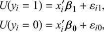 (3.1)
(3.1)
where
 is a set of actor-specific characteristics (explanatory variables) of actor
 ,
,
 and
and
 are
are
 vectors of coefficients with respect to choosing 0 and 1, and
 includes the error terms. Therefore, the probability of choosing
 is simply the probability of
 , which can be written formally as
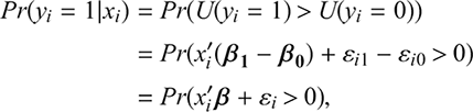 (3.2)
(3.2)
where
 and
and
 . Since the constant term in the latent utility specification is unchanged by the choice of switching thresholds, we can follow the conventional practice and normalize the utility of the second choice to 0. Consequently, we have the following latent utility specification:
 (3.3)
(3.3)
By adding a probability measure over Equation (3.3), it follows that
 (3.4)
(3.4)
Under symmetry of the error distribution, we can obtain the following form
 (3.5)
(3.5)
where
 is a cumulative distribution function. In general, the conditional mean-based regression for binary outcomes assumes the following form
 (3.6)
(3.6)
This formulation summarizes the relationship through a single conditional index and therefore cannot directly represent heterogeneity across different parts of the latent response distribution (Lu, Reference Lu2020).
Besides the above limitation, the mean-based discrete choice models can produce systematic prediction errors when the assumption of independence of irrelevant alternatives is violated or when the distribution of the error term is misspecified. These two constraints will be elaborated in the subsequent discussions.
3.2.1 Independence of Irrelevant Alternatives
In broader discrete-choice settings, standard logit models often rely on the independence of irrelevant alternatives (IIA) assumption, which follows from particular assumptions about the stochastic components of utility across alternatives. This assumption implies that when considering any two alternatives, the addition of further alternatives will not alter the probability ratio between them. This can be represented formally by the following equation:
 (3.7)
(3.7)
which means that the probability ratio (or odds ratio) of choosing 1 over 0 given the set of alternatives
 is the same by adding an additional alternative 2 to the original set of alternatives
 .
.
The IIA assumption becomes stringent in cases where, for instance, alternatives 0 and 2 exhibit similar characteristics while alternative 1 stands out. In such situations, the probability of selecting 0 decreases due to the presence of a comparable alternative 2, but the probability of choosing 1 remains relatively unchanged. Consequently, the probability ratio between 1 and 0 increases because of the existence of alternative 2, thus violating the IIA assumption.
As a more concrete example, consider vote choices in multi-party systems. When examining voting behavior in such systems, the emergence of a third party with an ideological position closely aligned with one of the two existing parties will inevitably impact voters’ choices among the three parties. Specifically, the presence of the new party is likely to decrease the election chances of the party that shares a similar ideology.
When the IIA assumption is violated, conventional mean-based discrete choice models like logit and probit may lead to biased inferences. While the violation of the IIA assumption is less consequential in binary choice settings, it becomes a problem with the presence of multiple alternatives, which will be examined in Section 4.
3.2.2 Potential Distributional Misspecification of Mean-Based Binary Models
The most commonly used binary models, such as logit and probit models, are restricted by their relatively rigid distributional assumptions. To convert a linear combination of covariates with complete support over the real line to a probability space ranging from zero to one, traditional binary models use a certain type of cumulative distribution function as the link function. The most common choices of the cumulative distribution function are the normal cumulative distribution, which gives rise to the probit model:
 (3.8)
(3.8)
and the logistic cumulative distribution, which is the core of the logit model:
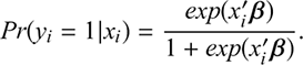 (3.9)
(3.9)
However, these distributional assumptions are substantively stringent and may lead to inaccurate estimations. To demonstrate potential bias that can be generated when the underlying error distribution differs from the assumed one, we can simulate a simple dataset in the following form:
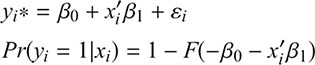 (3.10)
where
 ,
,
 ,
,
 , and
, and
 are the cumulative distributions with the error term assuming respectively the following seven distributions (Lu, Reference Lu2020):
Distribution 1: Normal distribution:

Distribution 2: T distribution with 3 degrees of freedom
Distribution 3:
distribution with 3 degrees of freedomDistribution 4: Asymmetric Laplace distribution (location 0 and scale 1)
Distribution 5: Kurtotic distribution from a weighted mixture of normal distributions
Distribution 6: Bimodal distribution from a symmetric mixture of normal distributions
Distribution 7: Skewed distribution with a mixture of three normal distributions





Estimating the data with the above distributions by the probit model, Figure 12 shows that except for the correctly specified model in the top-left panel (distribution 1), the probit model can deviate noticeably from the true response probabilities under alternative latent error distributions. For example, for the estimation of the data with the skewed distribution of the error term, the probit model under-predicts the probabilities in lower values of
 . However, it is more likely to overpredict the probabilities when the error term follows the bimodal distribution. This indicates that in the discrete choice settings, the specification of error terms matters. Once the underlying distribution deviates from the assumption, the estimator is likely to produce biased estimates.
Comparison between the predicted probabilities and the true probabilities under different error distributions
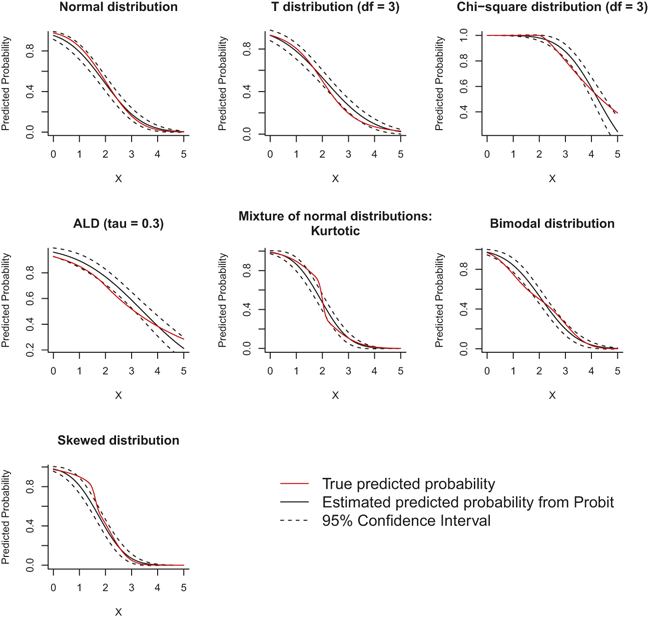
Compared to the mean-based discrete choice models, quantile models adopt more flexible distributional assumptions and are thus more robust to distributional misspecifications. For the binary choices, the following section will introduce the technical details of the binary quantile model.
3.3 Binary Quantile Model
Mean-based discrete choice models, including the logit and probit models, are commonly used to analyze data with discrete outcomes. However, as demonstrated earlier, these conventional mean-based models impose strong assumptions about data distributions and are likely to overlook heterogeneity among individuals or subgroups of a population. In many research situations, we are interested in how explanatory variables operate across the latent response distribution beyond just the conditional mean.
Quantile models represent a particularly useful approach for this purpose. For a binary response variable, we assume that a latent continuous variable
 determines the observed binary outcome
 . Therefore, a coefficient
 from the quantile estimation represents the change in the
 th quantile of the latent propensity
 for a one-unit increase in predictor
 , holding other variables constant. Coefficients at higher quantiles reflect effects on observations with high latent propensity, while coefficients at lower quantiles reflect those with low latent propensity. Thus, unlike mean-based binary models, the binary quantile model captures heterogeneous effects across the latent propensity distribution.
For binary outcomes, the quantile-regression logic cannot be applied directly to the observed response in the same way as in the continuous case, and estimation therefore requires a latent-variable formulation together with simulation-based methods. To handle the problem, scholars have begun to explore the advantages of the Bayesian approach for quantile estimation (Benoit, Alhamzawi, & Yu, Reference Benoit, Alhamzawi and Yu2013; Benoit & Van den Poel, Reference Benoit and Van den Poel2012; Florios & Skouras, Reference Florios and Skouras2008; Kordas, Reference Kordas2006). In particular, Benoit and Van den Poel (Reference Benoit and Van den Poel2012) developed a simulation-based estimator for binary quantile models that draws posterior samples through the MCMC process. This approach allows inference of parameter values from the joint posterior distribution, without the need to adopt ad hoc approximation methods.
Because the minimizing problem in Equation (2.5) is closely related to the asymmetric Laplace distribution (ALD) (Koenker & Machado, Reference Koenker and Machado1999), it is possible to estimate the quantile regression within the framework of the ALD distribution. The ALD density of a random variable
 conditioning on three parameters,
 ,
,
 , and
, and
 , can be written as
 (3.11)
where
 is determined by the specified quantile, and
 containing the covariates is the main parameter of interest (Yu & Zhang, Reference Yu and Zhang2005). Compared to other commonly used distributions for mean-based discrete choice models, the ALD is more flexible in the sense that it can easily adjust the skewness, shape, and location by varying the values of the parameters. In a discrete choice setting, the dispersion parameter
 is normalized to 1 for identification.
By inserting a monotone indicator function, the quantile representation of the binary response variable given a set of covariates has the following form:
 (3.12)
where
 is an indicator function that takes the value of one when the condition within the bracket is satisfied, and zero otherwise. For a binary response variable
 , the probability of
 conditional on the data and the quantile is as follows:
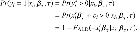 (3.13)
Instead of using Metropolis–Hasting within the Gibbs algorithm to sample the joint posterior distribution, the ALD can be represented as a location-scale mixture of normal distributions (Kotz, Kozubowski, & Podgorski, Reference Kotz, Kozubowski and Podgorski2001, Reference Kotz, Kozubowski and Podgorski2003; Kozumi & Kobayashi, Reference Kozumi and Kobayashi2011; Reed & Yu, Reference Reed and Yu2009; Yu & Moyeed, Reference Yu and Moyeed2001):
 (3.14)
where
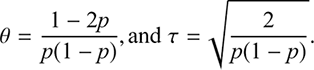 (3.15)
Here,
 denotes the skewness of the distribution. As a result, latent variable
 can be rewritten as
 (3.16)
where
 and
and
 are auxiliary variables. Consequently, we have the joint distribution given data as
 (3.17)
In the simple binary choice model, it is possible to augment the data in the sampling procedure by adding a latent variable
 , which has continuous support over the whole real line:
 (3.18)
As a result, the inference of
 is simply the integral of latent variable
 :
:
 (3.19)
The estimation procedure following the above calculations has been incorporated into an R package bayesQR (Benoit & Van den Poel, Reference Benoit and Van den Poel2017). Thus, rather than dwelling on the details of the sampling methods, the following section will demonstrate the application of the binary quantile model using a real-world political example on the EU policymaking.
3.4 Example of Binary Choices: EU Policymaking
To illustrate the application of the binary quantile model, this section considers an example of policymaking in the European Union. In 1992, the Maastricht Treaty established the so-called codecision legislative procedure, which requires the Council of the European Union to negotiate with the European Parliament (EP) in order to pass a bill. While the introduction of the codecision procedure empowered the EP to enhance the democratic process, the Amsterdam treaty of 1999 amended the procedure to allow legislation to be concluded as early as in the first reading stage. This reform raised trade-offs between democracy and efficiency, and gave the colegislators the option of concluding legislation earlier or later in the process. The potential for concluding a bill early in the EU legislative procedure has led to more frequent informal meetings and sparked the concern that a biased rapporteur, who acts as the EP’s representative, might exploit this opportunity to advance personal policy goals at the expense of the whole EP (Farrell & Héritier, Reference Farrell and Héritier2004).
To study the conditions under which colegislators, that is, the Council and the EP, decide to conclude an early agreement, Rasmussen (Reference Rasmussen2011) proposes three sets of factors that may influence early conclusion of EU legislative bills, namely, the delegation costs of the rapporteurs from the EP, the bargaining certainty, and the bargaining impatience. While the first factor is expected to reduce the likelihood of a first reading agreement, the latter two factors are hypothesized to increase the likelihood. The empirical results from the ordinary logit regression lend support to the three proposed hypotheses.
However, the ordinary logit model originally used by the author is unable to account for the potential heterogeneity in the EU codecision bills. For example, the impact of delegation costs on early agreement may differ depending on each bill’s latent propensity to be concluded through a fast-track procedure. For conflictual bills that are less likely to be included in fast-track legislation or trivial bills where consensus among legislators is easy to reach, it is reasonable to expect that the impact of delegation costs on early agreement will be low (Lu, Reference Lu2020). Yet, for bills that have neither a very low nor a very high likelihood of being concluded early in time, we would expect a more significant impact of delegation costs.
To demonstrate the new insight that could possibly be generated from the quantile approach, I replicate the original analysis in this section by applying the binary quantile model (see also Lu, Reference Lu2020). In the model, the conditional quantiles represent varying latent propensity of early agreement for different bills. Although the IIA assumption is not relevant in this case as there are only two choice alternatives (early conclusion of a bill or not), the key issue lies in the identification of unobserved heterogeneity among legislative bills. Even by controlling for potential confounding variables in the mean-based model, it still provides no guarantee that unobserved heterogeneity among bills and their local effects has been well accounted for. To identify unobserved heterogeneity and promote our understanding of the lawmaking in the EU, I focus on the full model (Model III in table 2 and figure 4 of the original paper by Rasmussen (Reference Rasmussen2011)) and estimate the data using the binary quantile model, with specified quantiles ranging from 0.1 to 0.9.
Using a cleaned version of the original dataset, the following codes load the ready-for-estimation data into the memory and carry out a brief preliminary inspection.Footnote 12
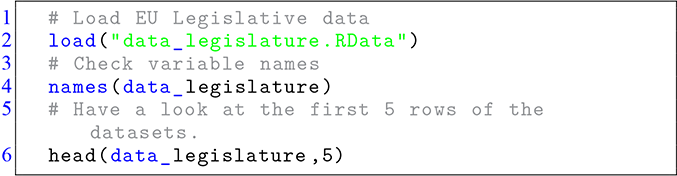
Code 1.8
1 # Load EU Legislative data
2 load("data_legislature.RData")
3 # Check variable names
4 names(data_legislature)
5 # Have a look at the first 5 rows of the  datasets.
6 head(data_legislature,5)
To implement the simple binary quantile estimation, we can use the bayesQR function provided by the package of the same name.Footnote 13 The following codes demonstrate the estimation procedure, where the estimation results are stored in the object mod1, which can be further assessed using the function summary. It is also possible to predict the responses relying on the estimated coefficients using the function predict.
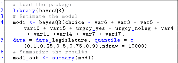
Code 1.9
1 # Load the package
2 library(bayesQR)
3 # Estimate the model
4 mod1 <- bayesQR(choice ~ var6 + var3 + var5 + var10 + var15 + urgcy_yes + urgcy_noleg + var4 + var11 +var14 + var7 + var17,
5 data = data_legislature, quantile = c(0.1,0.25,0.5,0.75,0.9),ndraw = 10000)
6 # Summarize the results
7 mod1_out <- summary(mod1)
As the Bayesian procedure is used for the estimation of the binary quantile model, we have to check whether the MCMC chains of the estimates have converged before proceeding to the interpretation of the results. This can be done by creating traceplots with the following functions.

Code 1.10
1 # Traceplot of MCMC draws
2 par(mfrow = c(2,3), mar = c(4, 4, 1, 2))
3 plot(mod1, var = "var3", plottype = "trace", burnin = 100,main = "",ylab = "Coefficient",xlab = "Iteration")
Figure 13 suggests satisfactory mixing and no obvious convergence problems. Consequently, we proceed with the substantive interpretation of the estimates.
Traceplot of MCMC draws
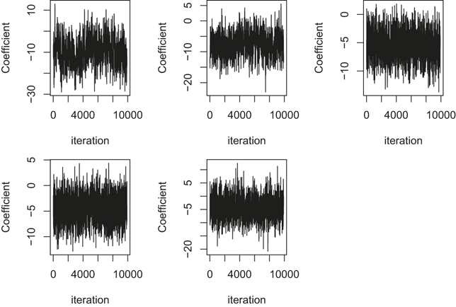
To examine, for instance, the estimated coefficients of the distance between the rapporteur and the EP median (i.e., the delegation costs), Figure 14 presents the quantile coefficient plot. While the logit model indicates a significantly negative average estimate, the quantile models reveal different effects at the lower and upper quantiles of the latent propensity for early agreement. More specifically, the figure shows that, although the median (0.5th quantile) effect mirrors the significantly negative mean estimate, there are no significant effects at the lower (0.1th quantile) and upper (0.9th quantile) ends of the latent early agreement propensity.
Coefficients of distance between rapporteur and EP median
Note: The black dotted line and the shaded area represent the quantile estimates and their 95% credible intervals, while the solid lines represent the estimates by the logit model with 95% confidence interval.
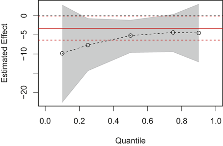
These estimates suggest that compared to an average bill, the effects of the subgroups of bills at the tails of the distribution of the response variable can be quite different. Substantively, it indicates that for contested bills that are unlikely to be concluded early in the EU legislative process, or trivial technical bills that are mostly decided by technocrats behind closed doors, the impact of potential policy deviation of negotiators on early conclusion can be different compared to other ordinary bills. In other words, the negative impact of biased policy negotiators on early conclusion of a bill only holds if the bill under consideration is neither very likely nor very unlikely to be considered as a fast-track legislation for early agreement. Therefore, the concern about the policy influence of a biased rapporteur in the fast-track legislation is only partially eliminated for those average bills, but not for bills at the tails of the distribution. The quantile finding also implies that the inclusion of bills in the fast-track procedure is a strategic decision of the EU legislators depending on the nature of the bills, and thus provides new insight – that would have remained unexplored using the conditional mean-based model – for understanding the legislative activities in the EU.
For the comparison of model performances between the ordinary logit model and binary quantile models, we can predict probabilities based on the estimates, and compare the predicted choices with the observed outcomes.

Code 1.11
1 predict(mod1,X = data_legislature,burnin = 100)
The results show that compared to the 76.6% prediction accuracy of the ordinary logit model, the prediction accuracies of the binary quantile model in nine quantiles range from 75.1% to 77.7%. Five out of nine quantile predictions perform equal to or better than the ordinary logit model. More importantly, however, the substantive gain of the quantile approach lies not primarily in prediction, but in its ability to uncover heterogeneity in the relationship between covariates and early agreement.
To further examine the effects of other variables, we can also plot for all covariates the coefficient estimates and their uncertainty (Lu, Reference Lu2020). In essence, if unobserved heterogeneity has been well controlled for, we should expect no large variation among different quantile estimates. However, as shown in Figure 15, the variation is large for the quantile estimates of many variables that have been included in the analysis. This indicates that compared to the ordinary logit model, quantile models are more useful for the examination of the heterogeneous relationship between those covariates and the response variable.
Quantile coefficient plot for all variables in EU policymaking example
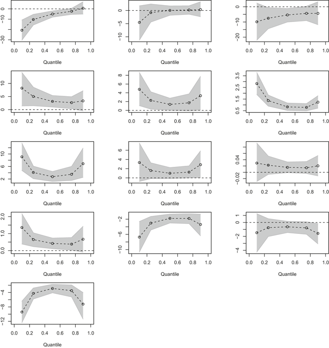
If we look more closely into the details of the estimation results, we can find that the predicted probabilities at quantiles 0.1 and 0.9 have the smallest reductions when delegation costs are measured by the distance between the rapporteur and the EP median. This reinforces the interpretation that the EU colegislators are less concerned about delegation costs when the bills are very likely or unlikely to be concluded early in time. Such bills, for example, include those that are of an administrative nature and thus need no further negotiation, or those on which it is difficult for member states to reach a compromise, and consequently, they reach no agreement at all. These are significant insights that emerge from estimating quantile models, which are likely to be overlooked if one relies solely on mean-based models.
3.5 Summary
Discrete response variables, such as the presence of conflicts, the voting behavior of electorates, and the success or failure of legislative bills, are often central to empirical political research. Despite the common occurrence of discrete choice data, most applications of quantile methods concentrate on continuous response variables, leaving the discrete case comparatively less explored. This section has shown that the quantile perspective can also be extended to binary choice settings, where it provides a useful complement to conventional mean-based models. Rather than summarizing behavior solely through conditional choice probabilities, the binary quantile model allows researchers to examine heterogeneity across the latent response distribution underlying observed choices.
Focusing only on average effects can provide an incomplete account of political behavior when the underlying process is heterogeneous. In binary settings, this problem does not disappear simply because the observed outcome takes values of zero and one. What matters is that the latent propensity toward the outcome may vary systematically across observations, and that explanatory variables may affect different parts of that latent distribution in different ways. Binary quantile models are valuable because they make such variation visible.
From the EU legislative example, it is evident that compared to an average bill, the EU legislators are less concerned about the delegation costs of bills that are either very likely or very unlikely to be passed early. These bills typically pertain to technical matters or involve contentious political issues. Thus, even in the simple two-alternative cases, unobserved heterogeneity justifies the use of quantile models. These models effectively capture heterogeneity in the effects of main explanatory variables, therefore providing new insights on the EU lawmaking process.
The application of quantile models for discrete choice data is not limited to binary cases. In the following section, it extends the discussion to quantile models for analyzing multiple alternatives, and for cases where there might also be alternative specific-features in choice sets.
4 Quantile Models for Multiple Choices
4.1 Introduction
The simple binary choice framework discussed in the previous section is useful for simple two-alternative settings, but many political decisions involve more complex choice environments. In political research, for example, we frequently analyze observational datasets where decision-makers operate under heterogeneous decision-making contexts, characterized not only by distinct option menus across cases but also by intra-case variability in available alternatives. In such settings, a model designed for simple binary outcomes is no longer sufficient. A useful way to address this problem is to reformulate multi-alternative choice as a set of conditional binary comparisons within each choice set. This is the logic behind the conditional binary quantile (CBQ) model, which extends quantile analysis to settings with multiple alternatives and alternative-specific features (Lu, Reference Lu2020).
In the context of binary choices, the conditional probability that a specific alternative is selected from a choice set can be represented as the likelihood that the latent utility of this alternative surpasses that of the other option. However, with the increasing number of choice alternatives, the probability calculation becomes more complicated. Consequently, additional statistical procedures are necessary to incorporate multiple alternatives and account for alternative-specific features, which will be introduced in the following sections.
4.2 Incorporation of Multiple Alternatives and Alternative-Specific Features
Consider the following example with three alternatives in a choice set
 . The probability of choosing
 given a set of covariates
 is the probability that the utility from alternative 1 is greater than those of alternatives 2 and 3:
 (4.1)
(4.1)
where
 collects the alternative-specific covariates for all three options in choice set
 (Lu, Reference Lu2020). Modeling the random component in a latent linear specification
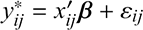 , we can rearrange the equation and rewrite the conditional probability as follows:
 (4.2)
(4.2)
where
 denotes the joint probability density function of
 and
and
 (Lu, Reference Lu2020).
We can simplify the above equation by modeling the difference between two random components as a single random variable:
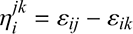 . More generally, let
 denote
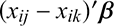 ; the probability of choosing alternative
 in the choice set with the number of alternatives
 can be expressed as an integral over the joint distribution of all pairwise error differences relative to
 (Lu, Reference Lu2020):
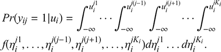 (4.3)
(4.3)
This representation makes clear that, once more than two alternatives are present, the choice probability depends on a joint comparison across all available options rather than on a single binary threshold. To formulate an appropriate likelihood function, a multinomial structure can be embedded in the calculation of the joint probability (McFadden, Reference McFadden and Zarembka1974). To do so, the probability for each alternative is weighted by the number of choice alternatives in the corresponding choice set. Each weight is formulated as
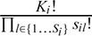 , where
 is the number of alternatives in choice set
 , and
, and
 is the number of alternatives
 in choice set
 with the total number of alternatives
 . This leads to the following conditional likelihood function given
 choice sets (Lu, Reference Lu2020):
 (4.4)
(4.4)
Equation (4.4) is a general form of the conditional binary choice model. This general framework encompasses the CL model (McFadden, Reference McFadden and Zarembka1974), the conditional probit model (Hausman & Wise, Reference Hausman and Wise1978), and the mixed logit (MXL) model (Hensher & Greene, Reference Hensher and Greene2003). However, in contrast to these models, the CBQ model relies on less restrictive distributional assumptions and does not depend on the IIA assumption. Compared to the conditional probit model, the CBQ model offers a comparatively parsimonious way to study heterogeneity across the latent utility distribution.
To estimate the CBQ model, the data augmentation procedure as introduced in the simple binary setting cannot be directly applied due to multiple alternatives in each choice set. As a result, there is no clear-cut threshold for the latent utility function. To deal with the problem, the estimation proceeds via the joint posterior density of all random components in the model, which can be formulated as
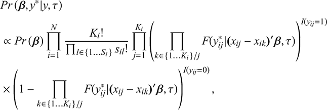 (4.5)
(4.5)
where
 is the cumulative distribution function of the ALD,
 is the number of choice sets,
 is the number of alternatives in the choice set
 , and
, and
 is the number of alternatives
 in the choice set
 , with the total number of alternatives
 (Lu, Reference Lu2020). The posterior distribution can then be sampled using a gradient-based MCMC algorithm (Hamiltonian Monte Carlo) that provides an efficient sampling routine (Hoffman & Gelman, Reference Hoffman and Gelman2014).
For applied research, there is already a statistical software that wraps up the above estimation equations into an easy-to-use R package (Lu, Reference Lu2020). The corresponding package for estimating the CBQ model, cbq is available in the CRAN, which can be downloaded by executing in the R console the following line of code:

Code 1.12
1 install.packages("cbq")
2 # Load the package
3 library(cbq)
Note that when choice sets contain more than two choice alternatives, we need to specify the conditionality of the estimation by using choice-set indicators. Each choice set must have a unique indicator so that the estimator can identify the alternatives belonging to the same choice set and how they are correlated with each other.
In the package, the conditionality of the estimation on the choice-set indicators is formulated by a vertical bar immediately following the specification of the covariates: “y
 x
x
 indicator variable.” The model specification in the function “cbq” has the following patterns: While we can specify formula in the traditional form of “y
 x” for simple binary choices, for multiple choices with or without varying choice alternatives, choice-set indicators need to be supplied in addition to the above formula: “y
 x
x
 choice-set indicator.” Moreover, we can estimate fixed- or random-effects in the following form: “y
 x
x
 choice-set indicator
 fixed-effects
 random-effects.”
In the following, I will present two prominent real-world political examples to demonstrate the basic elements of the quantile estimation procedure for multiple choices. The applications will also show how to view and interpret the results in multiple-choice and varying-choice-alternatives settings.
4.3 Example of Multiple Choices: US Presidential Election in 1992
The first example concerns the US presidential election in 1992, a natural example of multiple choice. Compared to the simple binary choice setting, there are three alternatives in this example, namely Clinton, Bush, and Perot. Using a subsample of 909 respondents from the 1992 American National Election Study (Miller, Kinder, & Rosenstone, Reference Miller, Kinder and Rosenstone1993), Alvarez and Nagler (Reference Alvarez and Nagler1995) offer a thorough examination of the mainstream explanations for Clinton’s success, including the economic voting, the spatial voting, and the so-called “angry voting” hypotheses.Footnote 14 The results from their multinomial probit model show that economic perception is the dominant factor determining the election outcome. While issue and ideological distances between the electorate and the candidates have some explanatory power, they are unlikely to alter the result. In addition, the authors find that the “angry voting” hypothesis was not fully supported by the data.
In contrast to the ordinary logit model, the multinomial probit model employed in the analysis by Alvarez and Nagler (Reference Alvarez and Nagler1995) permits simultaneous examination of multiple choices. It also provides a correlation structure between random components of the utility function, thereby eliminating the restrictive IIA assumption (Hausman & Wise, Reference Hausman and Wise1978). This is particularly relevant in this example, as the presence of the third choice alternative may affect the voters’ utility of choosing other candidates, which would not be taken into account if the IIA assumption were to hold. However, the correlation structure included in the multinomial probit model only distinguishes preferences between choice alternatives and does not differentiate the heterogeneous preferences of individuals for each choice alternative. Thus, it leaves substantial room for the application of the quantile approach in this example.
To revisit the election from a quantile perspective, we can specify varying quantiles from 0.1 to 0.9 as in Lu (Reference Lu2020), which correspond to different points in the latent propensity distribution for choosing a given candidate. Here, the conditional quantiles represent varying latent propensity of voting for a specific candidate given a set of explanatory variables. Consequently, we can estimate effects of the covariates for each specified quantile. As an example, in the following codes, we estimate the 0.1th conditional quantile using the cbq function, with other options regarding the details of the MCMC sampling procedure set to default.Footnote 15
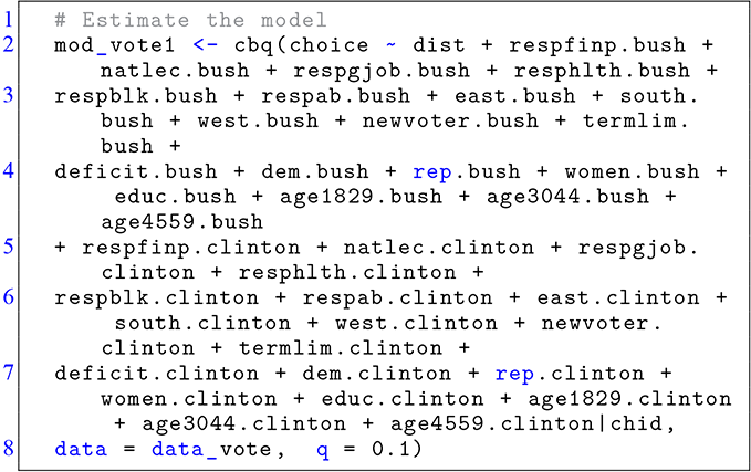
Code 1.13
1 # Estimate the model
2 mod_vote1 <- cbq(choice ~ dist + respfinp.bush + natlec.bush + respgjob.bush + resphlth.bush +
3 respblk.bush + respab.bush + east.bush + south.bush + west.bush + newvoter.bush + termlim.bush +
4 deficit.bush + dem.bush + rep.bush + women.bush + educ.bush + age1829.bush + age3044.bush + age4559.bush
5 + respfinp.clinton + natlec.clinton + respgjob.clinton + resphlth.clinton +
6 respblk.clinton + respab.clinton + east.clinton + south.clinton + west.clinton + newvoter.clinton + termlim.clinton +
7 deficit.clinton + dem.clinton + rep.clinton + women.clinton + educ.clinton + age1829.clinton + age3044.clinton + age4559.clinton|chid,
8 data = data_vote,  q = 0.1)
In the computational codes, the parameter “.
 chid” specifies the choice-set identifier. We can inspect the fitted object stored in mod_vote1 using the following lines of codes.
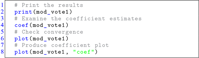
Code 1.14
1 # Print the results
2 print(mod_vote1)
3 # Examine the coefficient estimates
4 coef(mod_vote1)
5 # Check convergence
6 plot(mod_vote1)
7 # Produce coefficient plot
8 plot(mod_vote1, "coef")
By making a slight modification to the codes, it is straightforward to estimate more conditional quantiles of the data. In this analysis, I follow the usual practice by specifying nine equally spaced quantiles from 0.1 to 0.9.Footnote 16
To examine the performance of the models, the predict function can be used to calculate the predicted outcomes, and then compare them to the real observed values. Table 5 illustrates the confusion matrices generated respectively by the multinomial probit and the CBQ model at the 0.1th quantile. The values on the diagonal show the number of times the respective models correctly predicted the true election vote choices, and those off the diagonal show the number of incorrect predictions. While the predictions for the vote choices of Bush and Clinton are relatively similar between the two models, the prediction by the multinomial probit model for the choice of Perot is much worse than the prediction of the CBQ model at the 0.1th quantile. This suggests that the multinomial probit model appears to underpredict the voting probabilities for Perot at the lower quantiles, which are better estimated by the quantile model.
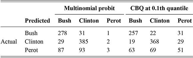
Table 5 Long description
The table presents confusion matrices comparing the prediction accuracy of a multinomial probit model and a C B Q model at the 0.1th quantile for three vote choices: Bush, Clinton, and Perot. Rows show actual vote outcomes, and columns show predicted outcomes. Diagonal values indicate correct predictions, while off-diagonal values indicate misclassifications. Both models perform similarly for Bush and Clinton votes, but the C B Q model predicts Perot votes more accurately than the multinomial probit model, highlighting that mean-based probit underestimates lower-quantile voting probabilities, which the quantile-based model captures better.
We can further compare the performance between the CBQ model and the multinomial probit model in the nine specified quantiles using the following codes.
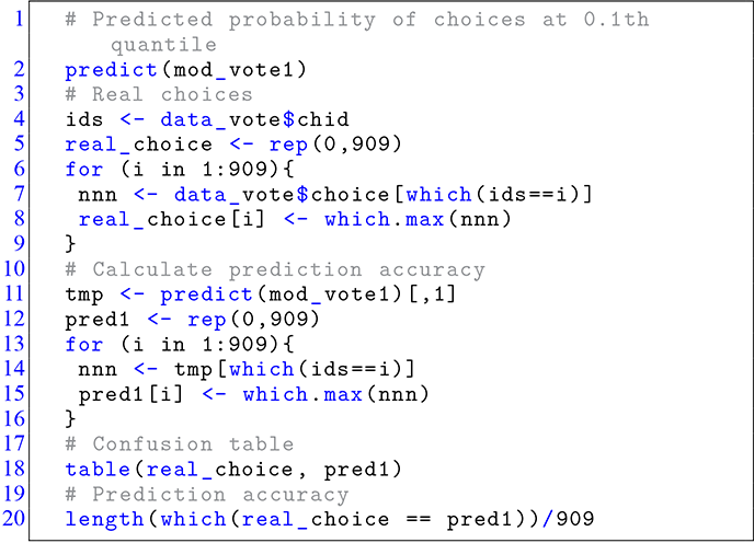
Code 1.15
1 # Predicted probability of choices at 0.1th quantile
2 predict(mod_vote1)
3 # Real choices
4 ids <- data_vote$chid
5 real_choice <- rep(0,909)
6 for (i in 1:909){
7 nnn <- data_vote$choice[which(ids==i)]
8 real_choice[i] <- which.max(nnn)
9 }
10 # Calculate prediction accuracy
11 tmp <- predict(mod_vote1)[,1]
12 pred1 <- rep(0,909)
13 for (i in 1:909){
14 nnn <- tmp[which(ids==i)]
15 pred1[i] <- which.max(nnn)
16 }
17 # Confusion table
18 table(real_choice, pred1)
19 # Prediction accuracy
20 length(which(real_choice == pred1))/909
Table 6 reveals that the prediction accuracies of the CBQ model at nine quantiles are all better than the prediction accuracy of the multinomial probit.
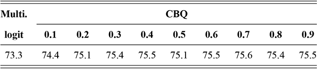
Table 6 Long description
The table shows the prediction accuracy (in percent) of the multinomial probit model and the C B Q model across nine quantiles (0.1 to 0.9). The multinomial probit achieves 73.3% accuracy, while the C B Q model ranges from 74.4% to 75.6% across the nine quantiles. The results indicate that the C B Q model consistently outperforms the mean-based multinomial probit, demonstrating the improved predictive performance of quantile-based modeling for election outcomes.
Besides a better prediction performance, the CBQ estimates show considerable variation across quantiles. To quantify the unobserved heterogeneity among voters for each choice alternative, we can calculate the standard deviation of nine quantile estimates for each covariate associated with the voters’ characteristics.Footnote 17
As shown in Table 7, the largest cross-quantile variation appears for the covariates Abortion, Democrat, Republican, and Respondents’ education. Everything else being equal, preference heterogeneity is low for those who identify themselves as Democrats when voting for Clinton. The same is true for those who identify as Republicans when voting for Bush, which is in line with the literature on party alignment (see, e.g., Miller, Reference Miller1991). However, when considering candidates from other parties, there is a considerable preference heterogeneity among voters. For example, in terms of abortion – a contentious issue during the election – pro-abortion voters have more coherent preferences when voting for Clinton rather than for Bush. This makes sense given the clear opposition of pro-abortion voters to Bush. Finally, even though educated voters tend to vote for Bush, they show higher heterogeneity in voting for Bush than in voting for Clinton (see also Lu, Reference Lu2020). These diverse characteristics uncovered by examining conditional quantiles offer a richer understanding of the voting patterns among distinct voter groups, which are overlooked by models relying on conditional means.
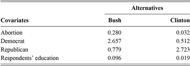
Table 7 Long description
The table reports voter heterogeneity measured as the standard deviation of quantile estimates for four covariates - Abortion, Democrat, Republican, and Respondents’ education - across two candidate alternatives, Bush and Clinton. Values indicate that heterogeneity is highest for Democrat identifiers when considering Bush (2.657) and for Republican identifiers when considering Clinton (2.723), reflecting strong alignment with party preferences. Abortion shows moderate heterogeneity for Bush (0.280) but low for Clinton (0.032), suggesting more coherent pro-abortion preferences for Clinton voters. Respondents' education exhibits low heterogeneity for both candidates (0.096 for Bush; 0.019 for Clinton). These results illustrate variation in voter preferences across issues and party lines, highlighting differences that conditional mean models may overlook.
To assess the estimated coefficients for each variable, we can generate quantile coefficient plots for every choice alternative (Bush and Clinton), excluding the reference alternative (Perot). The task can be accomplished with the following straightforward line of code.

Code 1.16
1 # Coefficient plot
2 plot(mod_vote1,"coef")
As Figure 16 shows, for the vote choice Bush, there is notable variation in the effects of most covariates across the distribution of the latent choice variable, i.e., the latent propensity of voting for Bush. Similarly, we can also plot the quantile coefficient values for vote choice Clinton, which is shown in Figure 17. This figure also shows a large variation in quantile effects of each covariate, which indicates significant heterogeneity in voting behaviors among American voters with diverse social, economic, and political backgrounds.
Estimated coefficients at quantiles ranging from 0.1 to 0.9 for US presidential election data with choice alternative Bush
Note: The estimates of variable Ideological Distance are the same between Bush and Clinton.
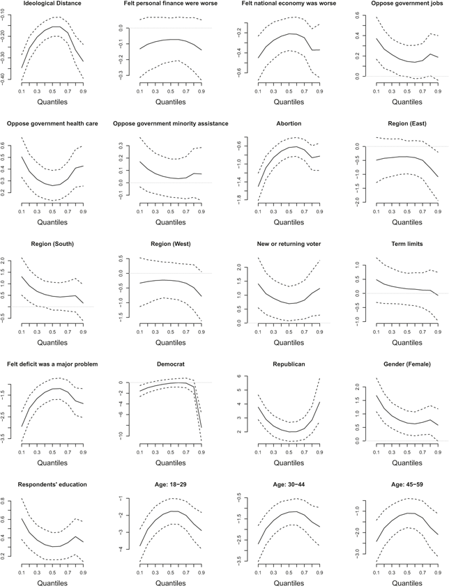
Estimated coefficients at quantiles ranging from 0.1 to 0.9 for US presidential election data with choice alternative Clinton
Note: The estimates of variable Ideological Distance are the same between Bush and Clinton.
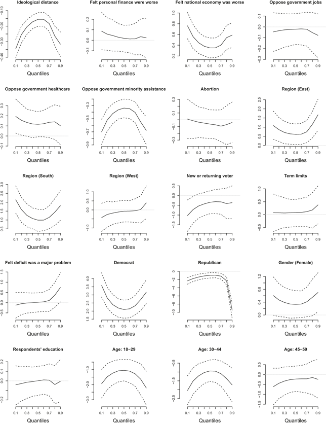
It is possible that unobserved heterogeneity among voters may affect the outcome of the vote when the ideological placement of the candidates changes. To draw a substantive interpretation of the estimation results, we can further compare the predicted vote shares of the three candidates by varying Bush’s position while keeping the other variables constant (Alvarez & Nagler, Reference Alvarez and Nagler1995). It also enables us to evaluate how the quantile and mean-based models perform when compared with the real outcomes.
Figure 18 shows the predicted vote shares of the three candidates by varying Bush’s position while keeping the other variables constant, with the solid lines representing the predictions of the multinomial probit model, and the dashed lines representing those of the CBQ model. The dots in the plot illustrate the actual vote share in the sample of the study. While the overall predictions are similar, the plot reveals that due to voter heterogeneity, the effects of the candidates’ ideological movement vary. The largest variation occurs when voters decide to vote for or against Perot. By comparing the predicted vote shares and the real vote shares, it is clear that the multinomial probit estimator does not well account for unobserved heterogeneity among voters. The multinomial probit model is among the worst predictors when Bush’s position is set at the actual value: 5.32. The best predictive quantile is 0.9, which suggests that loyal voters, who have a latent high propensity of voting for the corresponding candidate, have a greater influence on the final result than the rest of the voters. This finding suggests that, contrary to the conventional view emphasizing the importance of swing voters, the shift among core voters may have played a more significant role in determining the final result of the 1992 US presidential election. Thus, the underestimation of the multinomial model is likely due to the fact that it only estimates the average preferences and does not take into account the variation of the preferences between different types of voters.
Predicted vote shares of three candidates by varying Bush’s position
Note: The solid lines represent the predictions by the multinomial probit model, and the dashed lines represent the predictions by the quantile model.
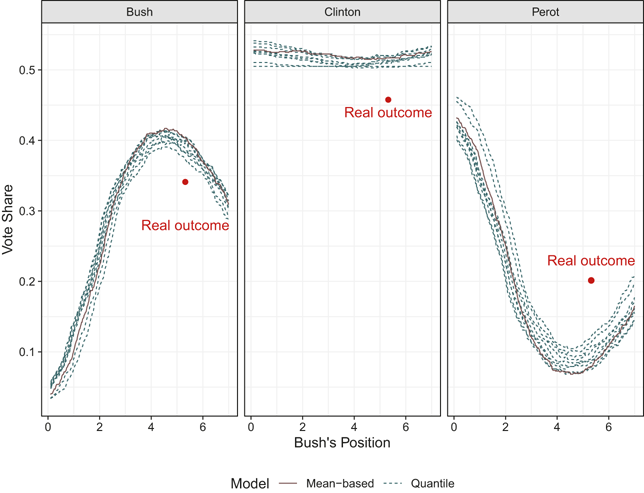
Taken together, the 1992 US election example illustrates how CBQ models can recover heterogeneity in multi-candidate choice settings that remains hidden in conventional multinomial models. By tracing covariate effects across the latent support distribution, the model not only improves predictive performance, but also yields substantively new insights into variation across types of voters. In this sense, the CBQ framework does more than refine existing estimates: it opens a different perspective on electoral behavior, one in which heterogeneous latent propensities matter directly for both explanation and prediction.
4.4 Example of Varying Choice Alternatives: Government Formation
Compared to the previous application of vote choices, the data structure of government formation in multi-party parliamentary democracies is considerably more complex. The number of feasible coalition alternatives varies across countries and legislative terms, and the composition of those alternatives differs sharply from one formation opportunity to another. For instance, while the United Kingdom often presents only a small number of plausible governing combinations, postwar coalition bargaining in systems such as Germany involves many more viable party constellations. To investigate the mechanisms of government formation, Martin and Stevenson (Reference Martin and Stevenson2001 have generated one of the most comprehensive government formation datasets, which contains a total of 220 formation opportunities and 33,256 potential governments in 14 parliamentary democracies between 1945 and 1987.
In the analysis of government formation, the numbers of coalition alternatives differ across countries and elections, and the characteristics of potential governments within each formation opportunity can be correlated. For example, the status of the minority coalition and the minimal winning coalition may depend on the inclusion or exclusion of the largest party in the coalition. Also, the coalition with the previous prime minister can be correlated with the status of the incumbent coalition. The IIA assumption is likely to be violated when unobserved government characteristics are correlated. This can happen when some government alternatives are substitutes or complements to each other. With a growing number of government alternatives, the risk of such correlation will also increase. Therefore, when estimating the traditional discrete choice model with equal weights over all coalition alternatives, a formation opportunity with a large number of coalition alternatives can distort the estimated formation likelihood of other coalitions.
To address variation in the number of coalition alternatives across cases, Martin and Stevenson (Reference Martin and Stevenson2001) propose to use the CL model, which accounts for varying formation opportunities across choice sets. However, the CL model relies on the strong IIA assumption, which is often violated in practice. In a later replication study, Glasgow, Golder, and Golder (Reference Glasgow, Golder and Golder2012) apply an MXL model to relax the restrictive IIA assumption and identify some disparities between their result and that of Martin and Stevenson (Reference Martin and Stevenson2001). Even so, both CL and MXL models assume a logistic form of the underlying error distribution and are thus restricted in assessing the full conditional distribution of the response variable (see the discussion in Section 3.2). They are therefore limited in their ability to reveal heterogeneity across the latent formation-propensity distribution. This is the setting in which the CBQ model becomes useful.
In the CBQ framework, conditional quantiles correspond to different points in the latent propensity distribution for successful coalition formation. The model therefore allows us to ask whether covariates matter differently for coalitions with relatively low, medium, or high latent probabilities of entering government. Although the underlying mathematics is more involved, estimation in practice is straightforward with the available software. The only additional requirement is that the model formula must include a choice-set identifier so that varying coalition alternatives are correctly grouped within each formation opportunity.
For a subset of the coalition formation data, the following codes estimate the 0.1th and 0.9th conditional quantiles while controlling for varying choice alternatives with a simple specification of the choice set indicator “.
 case” in the formula object.Footnote 18 Once estimation is complete, we can examine the estimates and their 95% credible intervals using the print function.
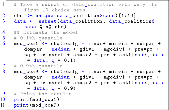
Code 1.17
1 # Take a subset of data_coalition with only the first 10 choice sets.
2 obs <- unique(data_coalition$case)[1:10]
3 data <- subset(data_coalition, data_coalition$case %in% obs)
4 ## Estimate the model
5 # 0.1th quantile
6 mod_coa1 <- cbq(realg ~ minor+ minwin + numpar + dompar + median + gdiv1 + mgodiv1 + prevpm + sq + mginvest + anmax2 + pro + anti|case, data = data, q = 0.1)
7 # 0.9th quantile
8 mod_coa9 <- cbq(realg ~ minor+ minwin + numpar + dompar + median + gdiv1 + mgodiv1 + prevpm + sq + mginvest + anmax2 + pro + anti|case, data = data, q = 0.9)
9 # Print the results
10 print(mod_coa1)
11 print(mod_coa9)
Based on the above estimation procedure, we can easily increase the number of estimated quantiles. Figure 19 shows the estimates of each covariate from 0.1th to 0.9th quantile. According to the figure, we can observe that the effects of most variables vary across quantiles. For example, while the effect of minority coalition remains significantly negative across quantiles, the magnitude decreases with increasing quantiles. Similarly, the positive effect of the largest party in the coalition decreases when a potential coalition becomes increasingly likely to be formed. These patterns suggest that average estimates obscure meaningful heterogeneity across different types of coalition alternatives.
Estimated coefficients at quantiles ranging from 0.1 to 0.9 for government formation data
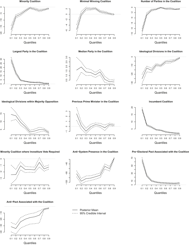
Since most potential governments are not actually formed, there is a potential risk that the prediction accuracy can be inflated when all potential governments are included in the estimation. With the increasing number of choice alternatives, the prediction accuracy will automatically increase, although nothing else has been changed. This can be problematic when we want to compare the actual performance of different models. Indeed, the prediction accuracies of all models are close to 99.2% when all potential coalition governments are considered.
To address this problem, instead of calculating the prediction accuracy of all potential coalitions, we can compare the predicted probabilities and the prediction accuracy of those governments that were actually formed (Lu, Reference Lu2020). For the 220 actually formed governments, the prediction accuracy of the CL and MXL models is 40.5% and 40%, respectively. The prediction accuracy of the CBQ model ranges from 34.5% to 42.3%. The best predictive quantiles are 0.1 and 0.9, with prediction accuracy of 42.3% and 40.9%, and the worst predictive quantiles are in the middle. This indicates that models centered on the middle of the latent distribution do not summarize all coalition types equally well, which further justifies the use of quantile models. Overall, compared to the quantile models, conditional mean-based models such as CL and MXL are restrictive in their capacities to capture unobserved heterogeneity of potentially promising (high quantiles) and very unpromising coalition governments (low quantiles).
To draw a substantive interpretation of the results, we can further perform counterfactual analysis by setting substantively meaningful scenarios. However, due to the complex data structure of varying choice alternatives, the traditional counterfactual analysis cannot be easily applied in the context of coalition government formation. As Glasgow, Golder, and Golder (Reference Glasgow, Golder and Golder2012) have pointed out, varying a single variable while keeping the others constant is likely to produce illogical results. Following the advice, we can create logically coherent counterfactual scenarios by switching the largest party to the second-largest party, which consequently leads to changes in the features of other potential governments (Lu, Reference Lu2020). The predicted probabilities of each model are then calculated from this logically coherent counterfactual dataset.
Using the full sample, Figure 20 plots the substitution patterns and compares changes in the predicted probabilities between CBQ and CL and between CBQ and MXL (see also figure 5 in Lu, Reference Lu2020). The upper panels show the comparison between CBQ and CL, and the lower panels show the comparison between CBQ and MXL. The hollow points represent pairs of changes in the predicted probabilities when the largest party becomes the second-largest party. Black points are pairs whose differences are statistically significant at the 95% confidence level, and gray points are those that are insignificant. The dashed lines are 45-degree lines on which the changes in probabilities are the same.
Comparing substitution patterns of CBQ, CL, and MXL models (see also Figure 5 in Lu, Reference Lu2020)
Note: The dashed lines are the 45-degree equal-division lines. Black points represent the pairs that are significantly different at a 95% confidence level while the gray points are insignificant. Q1 and Q9 indicate 0.1th and 0.9th quantile estimators, respectively. The average difference is calculated based on significantly different pairs.
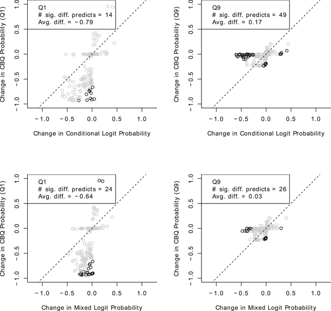
It is clear from the figure that the patterns between the upper and lower panels are very similar and that the main difference between the quantile models and the CL/MXL model comes from the lower (0.1th) and upper (0.9th) quantiles. For those significantly different pairs, the lower quantile predicts, on average, a negative change in probabilities, while CL and MXL predict almost no change. In contrast, the upper quantile predicts no change in probabilities, while CL and MXL predict, on average, a negative change. The different substitution patterns between the lower and upper quantiles indicate that potentially promising coalitions (those in the upper quantiles) and misery coalitions (those in the lower quantiles) respond differently than an average government when the largest party becomes the second-largest party. In particular, the promising coalitions suffer little from losing the largest party, while the misery coalitions’ chances of entering government decrease. However, this formation heterogeneity among different types of coalitions has not been captured by the conditional mean-based CL or MXL models.
To further account for potential confounders, we may also want to incorporate mixed effects (fixed and/or random effects) into the estimation of the CBQ model. To do so, we can modify the syntax to “y
 x
x
 indicator
 variable of fixed effects
 variable of random effects.” For example, if we are interested in estimating the random effects, the estimation formula can be specified as “y
 x
x
 indicator
 1
1
 variable of random effects.” For the coalition formation data, we can further incorporate country-fixed effects with two explanatory variables as follows.
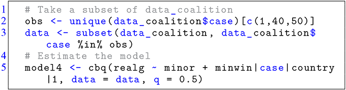
Code 1.18
1 # Take a subset of data_coalition
2 obs <- unique(data_coalition$case)[c(1,40,50)]
3 data <- subset(data_coalition, data_coalition$case %in% obs)
4 # Estimate the model
5 model4 <- cbq(realg ~ minor + minwin|case|country|1, data = data, q = 0.5)
Taken together, the coalition-formation example shows that mean-based choice models provide only a partial account of coalition bargaining when substantial unobserved heterogeneity is present across potential governments. The CBQ estimates reveal that many coalition characteristics have markedly different effects at different points of the latent formation-propensity distribution. The counterfactual analysis reinforces this conclusion: relatively promising and highly unlikely coalitions respond differently to changes in party composition, and these differences are obscured in mean-based models such as CL and MXL. In this setting, the quantile perspective does not merely refine existing estimates—it changes the substantive picture of how coalition alternatives compete to form governments.
4.5 Summary
This section has extended the quantile framework to discrete-choice settings with multiple alternatives and alternative-specific features. In particular, it introduces the CBQ model for assessing potential diverse effects at various points along the conditional response distribution when there are multiple alternatives in choice sets.
Examples from the US presidential election and coalition formation in parliamentary democracies are used to demonstrate the potential of quantile models in generating new theoretical and empirical insights. In the electoral example, the CBQ model reveals substantial heterogeneity across the latent support distribution and suggests that mean-based models miss important differences in how voters respond to candidates and issues. This heterogeneity is reflected not only in the estimated coefficients, but also in the improved predictive performance.
The coalition-formation example points to a similarly important form of heterogeneity. Coalitions with relatively high latent propensities of formation appear to respond differently to changes in party composition than coalitions in the lower tail of the distribution. In particular, the results suggest that highly promising coalitions are less affected by the loss of largest-party status than highly unlikely coalitions. Such differences are obscured by mean-based choice models, but become visible once the quantile perspective is introduced.
Overall, these examples show that CBQ models do more than refine estimation in multiple-choice settings. They open up new ways of analyzing political choice by allowing researchers to study how effects vary across the latent distribution of support, viability, or selection. The accompanying code and software implementations can be adapted to a wide range of applied research settings.
5 A Brief Overview of Other Quantile Methods
5.1 Introduction
It is straightforward to expand the quantile modeling approach for the analysis of political heterogeneity in research situations other than what has been introduced in the previous chapters. To demonstrate the broader applicability of quantile models besides the examples presented in the previous chapters, this section will explore briefly, but not exhaustively, some additional quantile techniques that could be helpful for political research. These include in particular quantile models for estimating quantile treatment effects and survival data. While they are relatively less frequently used than the quantile models introduced in the previous chapters, these quantile models can be helpful when researchers attempt to identify causal relationships from experiments, or study different types of response variables beyond those discussed so far.
In this section I will also introduce variable selection and model comparison in quantile settings. In addition to the benefits of quantile models, this section will discuss in the concluding section the practical suggestions for using the quantile approach, such as those related to the quantile interpretation, the sample size, and the selection of the number of quantiles.
Although this is by no means a complete overview of the rapidly developing field of quantile methods, this section is intended to demonstrate the wide applicability of quantile models to broader application situations of political research. For other quantile methods such as those concerning nonparametric quantile regression and quantile estimation of longitudinal and time series data that have been even less frequently used in political science, interested readers may refer to Koenker (Reference Koenker2017), Uribe and Guillen (Reference Uribe and Guillen2020), and Di Marzio, Panzera, and Taylor (Reference Di Marzio, Panzera and Taylor2016), among others, for further details of implementation.
5.2 Quantile Treatment Effects
Quantile treatment effects (QTEs) describe how the effect of a treatment varies across the outcome distribution (Frölich & Melly, Reference Frölich and Melly2013). In the potential-outcomes framework, the
 th QTE is defined as the difference between the
 th quantile of the treated outcome distribution and the
 th quantile of the untreated outcome distribution. In the simple case of a binary treatment
 and a continuous outcome
 , this can be written intuitively as:
 (5.1)
(5.1)
When a set of covariates
 can also be controlled for, one may consider conditional quantile treatment effects of the form
 (5.2)
(5.2)
In practice, the quantile treatment effects can be estimated by fitting quantile models for both treatment and control groups, and then comparing the estimated quantile-specific coefficients. This approach provides insights into how the treatment effect varies across different segments of the population, and thereby offers a more comprehensive understanding of the causal relations. The formula for estimating quantile treatment effects in the context of quantile regression can be expressed as follows:
 (5.3)
(5.3)
where
 is the treatment indicator variable, taking the value of 1 if the individual received treatment and 0 otherwise,
 is a set of controls, and
 captures the treatment contrast at quantile
 . The model assumes that the effect of treatment (
 ) on the conditional quantile of
 varies across different quantiles. Thereby, it allows for a more nuanced understanding of how the treatment effect changes at different points of the response distribution.
Estimating the quantile-specific coefficients and treatment effects follows the optimization procedure introduced in the previous chapters. Similar to the estimation procedure for observational studies, there are hands-on functions to estimate the quantile treatment effects when the data come from randomized experiments. The following example illustrates a slightly different but closely related use of quantile methods in experimental research: rather than estimating a treatment effect on the main substantive outcome, it uses quantile analysis to examine whether a key identification assumption holds uniformly across the response distribution.
As a real-world political example, consider a case study on vote buying in Nicaragua (Gonzalez-Ocantos et al., Reference Gonzalez-Ocantos, De Jonge, Meléndez, Osorio and Nickerson2012). Vote buying, or more generally political clientelism, is a pervasive phenomenon in the politics of the developing world (Kitschelt, Reference Kitschelt2000). However, due to potential social desirability and concerns about legal repercussions, many recipients of political gifts may not truthfully disclose their behavior. To mitigate response bias, Gonzalez-Ocantos et al. (Reference Gonzalez-Ocantos, De Jonge, Meléndez, Osorio and Nickerson2012) employed an indirect measurement technique called the “list experiment”. Rather than directly asking the respondents about sensitive issues like vote buying, this approach asks them to provide aggregate responses to a set of survey items that include the sensitive question (Blair & Imai, Reference Blair and Imai2012). However, using a list experiment comes at the cost of reduced estimation efficiency, limiting researchers to estimating only the prevalence rather than individual instances of sensitive behaviors from the data (Blair, Coppock, & Moor, Reference Blair, Coppock and Moor2020; Glynn, Reference Glynn2013).
To enhance the efficiency of estimation in list experiments, Aronow et al. (Reference Aronow, Coppock, Crawford and Green2015) propose to combine direct questions with list experiments, which significantly reduces the uncertainty in estimating behaviors such as vote buying (Lu & Traunmüller, Reference Lu and Traunmüller2026). However, ensuring accurate estimation through this method relies on the treatment independence assumption. This assumption posits that the assignment of treatment (i.e., inclusion in the list experiment treatment group) is independent of respondents’ answers to direct questions. In addition to placebo tests introduced by Aronow et al. (Reference Aronow, Coppock, Crawford and Green2015), we can examine the treatment independence assumption through quantile analysis between treatment assignment and responses to direct questions.
The rationale behind conducting quantile tests for the treatment independence assumption stems from the possibility of varying relationships between direct questions and treatment assignment across different segments of respondents. For example, individuals less likely to receive the treatment might also exhibit lower propensity to affirm the sensitive question in the direct form. Therefore, even if, on average, there is no discernible treatment effect on direct responses, the assumption of treatment independence could be compromised by significant effects in scenarios where treatment assignment probabilities differ. To explore potential heterogeneity of the treatment effect on direct responses, we can employ the quantile model by which the direct question is regressed against the treatment assignment. By estimating the relationship at different points along the distribution (quantiles), we gain insights into whether the assumption of treatment independence holds uniformly or if there are nuanced dependencies across different levels of the direct question’s response distribution. This approach allows us to detect any disparities in treatment effects that may exist among subgroups defined by their likelihood of affirming the sensitive question directly.
For the vote-buying example, Gonzalez-Ocantos et al. (Reference Gonzalez-Ocantos, De Jonge, Meléndez, Osorio and Nickerson2012) include in their list experiments also direct questions asking respondents whether they have received political gifts themselves (individual gifts) or are aware of some neighbors who have received gifts (neighbor gifts). Therefore, we can examine whether there are heterogeneous quantile treatment effects on the two direct questions. The following code presents the estimation procedure of both the simple binary choice model and the quantile models. For simplicity, the code estimates the models separately at each quantile. In practice, this can also be automated in a loop.
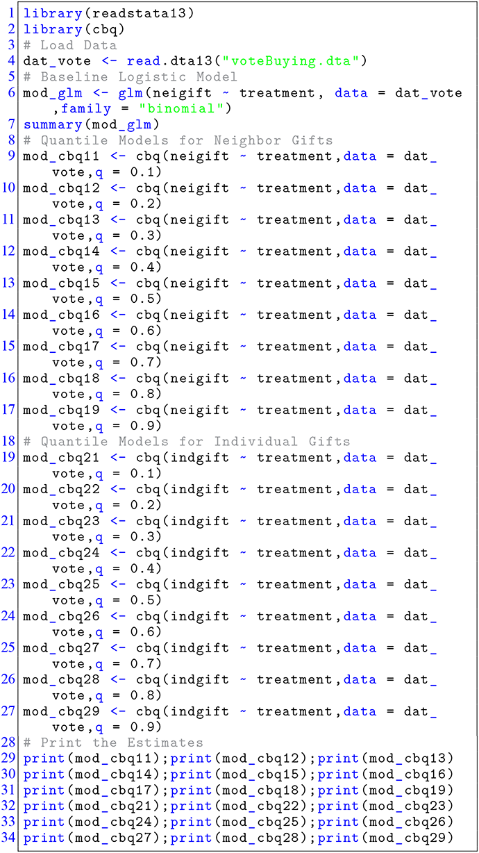
Code 1.19
1 library(readstata13)
2 library(cbq)
3 # Load Data
4 dat_vote <- read.dta13("voteBuying.dta")
5 # Baseline Logistic Model
6 mod_glm <- glm(neigift ~ treatment, data = dat_vote,family = "binomial")
7 summary(mod_glm)
8 # Quantile Models for Neighbor Gifts
9 mod_cbq11 <- cbq(neigift ~ treatment,data = dat_vote,q = 0.1)
10 mod_cbq12 <- cbq(neigift ~ treatment,data = dat_vote,q = 0.2)
11 mod_cbq13 <- cbq(neigift ~ treatment,data = dat_vote,q = 0.3)
12 mod_cbq14 <- cbq(neigift ~ treatment,data = dat_vote,q = 0.4)
13 mod_cbq15 <- cbq(neigift ~ treatment,data = dat_vote,q = 0.5)
14 mod_cbq16 <- cbq(neigift ~ treatment,data = dat_vote,q = 0.6)
15 mod_cbq17 <- cbq(neigift ~ treatment,data = dat_vote,q = 0.7)
16 mod_cbq18 <- cbq(neigift ~ treatment,data = dat_vote,q = 0.8)
17 mod_cbq19 <- cbq(neigift ~ treatment,data = dat_vote,q = 0.9)
18 # Quantile Models for Individual Gifts
19 mod_cbq21 <- cbq(indgift ~ treatment,data = dat_vote,q = 0.1)
20 mod_cbq22 <- cbq(indgift ~ treatment,data = dat_vote,q = 0.2)
21 mod_cbq23 <- cbq(indgift ~ treatment,data = dat_vote,q = 0.3)
22 mod_cbq24 <- cbq(indgift ~ treatment,data = dat_vote,q = 0.4)
23 mod_cbq25 <- cbq(indgift ~ treatment,data = dat_vote,q = 0.5)
24 mod_cbq26 <- cbq(indgift ~ treatment,data = dat_vote,q = 0.6)
25 mod_cbq27 <- cbq(indgift ~ treatment,data = dat_vote,q = 0.7)
26 mod_cbq28 <- cbq(indgift ~ treatment,data = dat_vote,q = 0.8)
27 mod_cbq29 <- cbq(indgift ~ treatment,data = dat_vote,q = 0.9)
28 # Print the Estimates
29 print(mod_cbq11);print(mod_cbq12);print(mod_cbq13)
30 print(mod_cbq14);print(mod_cbq15);print(mod_cbq16)
31 print(mod_cbq17);print(mod_cbq18);print(mod_cbq19)
32 print(mod_cbq21);print(mod_cbq22);print(mod_cbq23)
33 print(mod_cbq24);print(mod_cbq25);print(mod_cbq26)
34 print(mod_cbq27);print(mod_cbq28);print(mod_cbq29)
Figure 21 shows the estimation results. For both the individual and neighbor gifts shown in the left and right panels of the figure, we find no significant treatment effects across all the specified quantiles from 0.1 to 0.9. This provides strong evidence that the treatment independence assumption is unlikely to be violated in this example and that direct questions can reasonably be combined with the list experiment, as long as the underlying bias of the direct questions is properly controlled for (Lu & Traunmüller, Reference Lu and Traunmüller2026).
Estimates of quantile treatment effects
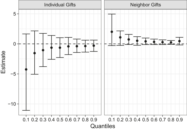
The above example illustrates one simple application where the estimation of quantile treatment effects can help to reveal the distributional structure of the relationship between the treatment and response variable of interest. Under nonexperimental environments, quantile treatment effects may also be identified with other techniques such as the instrumental variable quantile regression (Abadie, Angrist, & Imbens, Reference Abadie, Angrist and Imbens1998; Chernozhukov & Hansen, Reference Chernozhukov and Hansen2005; Frölich & Melly, Reference Frölich and Melly2010). Interested readers may refer to the relevant packages, such as “IVQR” and their documentation, for further implementation details.
5.3 Quantile Model for Survival Data
Quantile models can also be applied to various types of response variables other than the ones illustrated in the previous chapters. One such response variable commonly encountered in political research is the time until a certain political event occurs, which is the subject of classical survival analysis. This section will thus demonstrate the use of quantile models for the analysis of survival data.
Quantile models for survival analysis extend the basic quantile framework to handle censored survival time data. Instead of modeling the hazard function, quantile models for survival analysis can be formulated as a generalization of the accelerated failure time model, which models directly the time until an event occurs.Footnote 19 Thus, a positive coefficient means that an increase in the value of a covariate will increase the time until a certain event occurs. According to Peng and Huang (Reference Peng and Huang2008), given
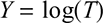 and under certain conditions, we can formulate the quantile survival model as follows:
 (5.6)
(5.6)
The concrete estimation procedure will additionally account for the censoring probability of each observation. Compared to the conventional survival model, such as the Cox proportional hazards model, the quantile regression approach allows for the estimation of quantile-specific effects in survival analysis, thereby providing a more detailed understanding of how covariates influence different points of the survival time distribution.
To demonstrate the application of quantile models for survival analysis in political science, take political responses to the COVID-19 pandemic in Europe as an example (Toshkov, Carroll, & Yesilkagit, Reference Toshkov, Carroll and Yesilkagit2022). In response to the rapid spread of the COVID-19 pandemic, national governments across Europe had introduced various public policy measures such as lockdowns, school closures, and mask-wearing requirements. The timing of these measures varies across countries and over time, and may be further influenced by a number of political factors such as government capacity, political institutions, and party ideologies (Toshkov, Carroll, & Yesilkagit, Reference Toshkov, Carroll and Yesilkagit2022).
To examine what accounts for the diversity of policy responses to the pandemic, Toshkov, Carroll, and Yesilkagit (Reference Toshkov, Carroll and Yesilkagit2022) collected a dataset on the announcement dates of anti-pandemic policies, including lockdowns and school closures, along with other explanatory variables such as government effectiveness, trust in government and type of government coalitions. Using their data, we attempt to examine in this example whether trust in government has varying effects on the timing of lockdowns depending on the relatively temporal location of each lockdown measure. Here, an event is an official announcement of the lockdown, and the response variable is the number of days between the first confirmed COVID-19 case in a country and the policy measure adoption (Toshkov, Carroll, & Yesilkagit, Reference Toshkov, Carroll and Yesilkagit2022).
As shown in Figure 22, with the elapsed time since the first confirmed COVID-19 case, the probability of no lockdowns decreases. In other words, the likelihood of imposing lockdowns after the confirmation of the first case increases over time. On average, the probability of introducing lockdown measures rises to 50% after 30 days since the first case, and it increases to almost 100% in 60 days. In fact, 23 out of 26 European countries included in the data had imposed lockdowns in 60 days since the first confirmed case. The estimation of the Cox proportional hazards model, which was adopted for the original analysis by Toshkov, Carroll, and Yesilkagit (Reference Toshkov, Carroll and Yesilkagit2022), further shows that trust in government will slow down the introduction of lockdown measures. This may be due to the ease of sustaining compliance with social distancing measures in a high-trust environment so that the pressure for the government to introduce lockdowns is relatively low (Toshkov, Carroll, & Yesilkagit, Reference Toshkov, Carroll and Yesilkagit2022).
Kaplan–Meier plot for introduction of lockdown measures
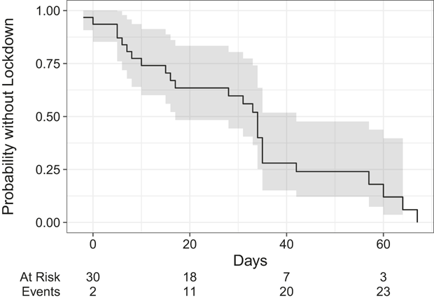
We can then proceed to analyze the potential heterogeneity in the effects of trust in government on the timing of lockdowns. Figure 23 shows the quantile estimation results for the survival data. Note that because the quantile models are performed on an accelerated failure time model (Portnoy, Reference Portnoy2003) instead of the Cox proportional hazards model, positive coefficient values imply negative impact on hazard rates. In this example, a positive estimate means that an increase in government trust will postpone the introduction of lockdown measures. While the estimates from lower to middle quantiles (0.1th–0.4th quantiles) correspond to the results of the Cox proportional hazards model, we cannot find any significant effect of government trust on the timing of lockdown measures in the upper quantiles (
 0.5th quantile).Footnote 20 This implies that when the introduction of lockdown measures has been delayed too long, the public trust in government will no longer play a role in influencing the timing of policy introduction. These heterogeneous effects are likely due to the increasing risk of pandemic spread without lockdowns. As a result, over a certain threshold of the infection rate, the government is forced to impose lockdowns regardless of the public trust in government, which explains the non-effect in the upper quantiles, where much time has passed without lockdowns since the first confirmed case. This is a substantively important pattern that would be obscured in a conventional hazard-based analysis.
Coefficient estimates of quantile model for lockdown example
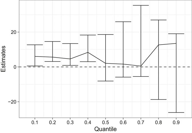
5.4 Variable Selection and Model Comparison
In many empirical studies, researchers may want to identify the most relevant variables from a larger set of potential predictors. By selecting the most important variables, we can simplify and improve the accuracy and interpretability of quantile models. Variable selection helps to reduce computational complexity, identify key variables that influence the response, and may also improve the generalizability of the model to new data.
To perform variable selection in quantile settings, researchers have extended penalization methods to quantile regression building on the logic of LASSO (Least Absolute Shrinkage and Selection Operator) (Tibshirani, Reference Tibshirani1996). It is an extension of quantile regression that includes a penalty term to enforce sparsity in the parameter estimates. The formula for LASSO quantile regression is expressed as follows:
 (5.7)
(5.7)
where
 is the regularization parameter that controls the strength of the penalty, and
 represents the absolute value of the
 -th coefficient in the vector
 . The first part of the formula,
 , is the quantile regression loss function, which measures the fit of the model to the data. The second part,
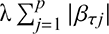 , is the LASSO penalty term that discourages large values of the coefficients. The objective is to find the values of
 that minimize the combined loss and penalty. The regularization parameter
 controls the trade-off between fitting the data well and keeping the parameter estimates sparse.
The optimization problem is typically solved using optimization algorithms, such as coordinate descent or proximal gradient methods, to find the values of
 that minimize the combined objective function. The rq function from the “quantreg” package allows for performing LASSO quantile model, where the method = "lasso" argument indicates the estimation of LASSO.
In the following example, we simulate a relatively homogeneous dataset with ten covariates, whose coefficients are
 for all values of
 . The codes estimating the LASSO quantile model are shown in the following.
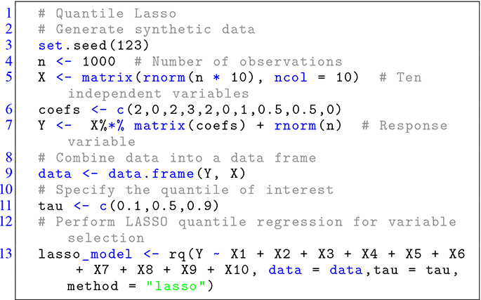
Code 1.20
1 # Quantile Lasso
2 # Generate synthetic data
3 set.seed(123)
4 n <- 1000  # Number of observations
5 X <- matrix(rnorm(n * 10), ncol = 10)  # Ten independent variables
6 coefs <- c(2,0,2,3,2,0,1,0.5,0.5,0)
7 Y <-  X%*% matrix(coefs) + rnorm(n)  # Response variable
8 # Combine data into a data frame
9 data <- data.frame(Y, X)
10 # Specify the quantile of interest
11 tau <- c(0.1,0.5,0.9)
12 # Perform LASSO quantile regression for variable selection
13 lasso_model <- rq(Y ~ X1 + X2 + X3 + X4 + X5 + X6 + X7 + X8 + X9 + X10, data = data,tau = tau, method = "lasso")
The results in the following code show that the LASSO quantile models at three specified quantiles all correctly shrink the coefficients of the covariates (X2 and X6) without discernible effects. This estimation procedure can be easily adopted for other political research situations in which researchers only need to input the regular model specifications.
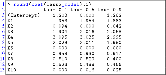
Code 1.21
1 > round(coef(lasso_model),3)
2 tau= 0.1 tau= 0.5 tau= 0.9
3 (Intercept)   -1.203    0.000    1.282
4 X1             1.953    1.954    1.883
5 X2             0.094    0.000    0.042
4 X3             1.904    2.016    2.058
5 X4             3.095    3.035    2.995
6 X5             2.029    2.011    1.980
7 X6             0.000    0.000    0.000
8 X7             0.958    0.930    0.917
9 X8             0.510    0.529    0.400
10 X9             0.523    0.488    0.466
11 X10            0.000    0.016    0.025
In addition to variable selection, model comparison in quantile regression can be done using various criteria, such as Root Mean Squared Error (RMSE), Mean Absolute Error (MAE), Check Loss (CL, a.k.a. Quantile Loss or Pinball Loss), Akaike Information Criterion (AIC), and Bayesian Information Criterion (BIC), among others. RMSE is a widely used metric to evaluate the accuracy of regression models. It measures the square root of the average squared differences between predicted and observed values:
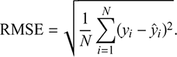 (5.8)
(5.8)
Similarly, MAE is a robust metric for evaluating regression model performance, which measures the average absolute differences between predicted and observed values:
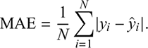 (5.9)
(5.9)
Unlike RMSE or MAE, which focus on central tendencies, the check loss allows modeling of any quantile by asymmetrically weighting residuals:
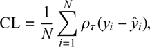 (5.10)
where
 is the check function as in Equation 2.4. In some settings, researchers also report information-criterion-style measures such as AIC or BIC. The AIC and BIC are measures of the relative quality of a statistical model for a given set of data. They penalize models based on the likelihood and the number of parameters, thereby balancing the trade-off between the goodness of fit and the complexity of the model (Akaike, Reference Akaike1987; Kass & Raftery, Reference Kass and Raftery1995; Schwarz, Reference Schwarz1978). The difference between the two measures is that AIC imposes a fixed penalty independent of sample size, while BIC’s penalty term grows with sample size:
 (5.11)
 (5.12)
where
 is the likelihood of the model,
 is the sample size, and
 is the number of estimated parameters. A lower AIC or BIC value indicates the better performance of a model. When comparing models, the model with the lowest AIC/BIC is generally considered the best, assuming that the models being compared are all based on the same data. Their use in quantile regression, however, is less straightforward than in standard likelihood-based models, and they are best treated as supplementary rather than primary criteria unless the underlying estimation framework provides a clear likelihood interpretation. In most applied quantile work, predictive criteria and quantile-specific loss functions are more directly informative.
Recall the study on the impact of economic crises on political representation introduced in Section 2. We can use the previously mentioned criteria to compare the performance of different quantile specifications. The estimation procedure is shown in the following codes:
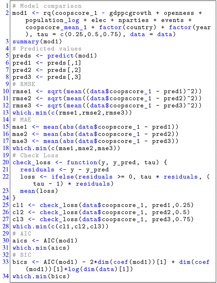
Code 1.22
1 # Model comparison
2 mod1 <- rq(coopscore_1 ~ gdppcgrowth + openness + population_log + elec + nparties + events + coopscore_mean_1 + factor(country) + factor(year), tau = c(0.25,0.5,0.75), data = data)
3  summary(mod1)
4  # Predicted values
5  preds <- predict(mod1)
6  pred1 <- preds[,1]
7  pred2 <- preds[,2]
8  pred3 <- preds[,3]
9  # RMSE
10  rmse1 <- sqrt(mean((data$coopscore_1 - pred1)^2))
11  rmse2 <- sqrt(mean((data$coopscore_1 - pred2)^2))
12 rmse3 <- sqrt(mean((data$coopscore_1 - pred3)^2))
13 which.min(c(rmse1,rmse2,rmse3))
14 # MAE
15 mae1 <- mean(abs(data$coopscore_1 - pred1))
16 mae2 <- mean(abs(data$coopscore_1 - pred2))
17 mae3 <- mean(abs(data$coopscore_1 - pred3))
18 which.min(c(mae1,mae2,mae3))
19 # Check Loss
20 check_loss <- function(y, y_pred, tau) {
21   residuals <- y - y_pred
22   loss <- ifelse(residuals >= 0, tau * residuals, (tau - 1) * residuals)
23   mean(loss)
24 }
25 cl1 <- check_loss(data$coopscore_1, pred1,0.25)
26 cl2 <- check_loss(data$coopscore_1, pred2,0.5)
27 cl3 <- check_loss(data$coopscore_1, pred3,0.75)
28 which.min(c(cl1,cl2,cl3))
29 # AIC
30 aics <- AIC(mod1)
31 which.min(aics)
32 # BIC
33 bics <- AIC(mod1) - 2*dim(coef(mod1))[1] + dim(coef(mod1))[1]*log(dim(data)[1])
34 which.min(bics)
In this illustration, RMSE favors the 0.75 quantile specification, whereas MAE favors the median model. Most of the remaining criteria also point toward the median quantile as the strongest single specification. This divergence is not surprising. Different criteria emphasize different aspects of model performance: RMSE penalizes large prediction errors more heavily, MAE is more robust to outliers, and check loss is tailored to the quantile objective itself. When the values are close across quantiles, as they are here, the practical conclusion is not that one quantile definitively dominates the others, but that several quantile specifications contribute useful information about the distribution.
For this reason, model-comparison statistics should be treated as helpful guides rather than as definitive arbiters of quantile choice. In substantive applications, it is usually more informative to estimate a grid of quantiles and to examine how the conclusions vary across the distribution than to rely on a single “best” quantile selected by one criterion alone. Model comparison should therefore complement, not replace, a broader distributional analysis.
5.5 Summary
This section has introduced several additional extensions of the quantile framework, including quantile models for estimating treatment effects and survival data. We have also discussed ways to select variables and compare models in quantile settings, thereby extending the practical toolkit introduced in the previous sections. However, despite the ability of quantile models to capture the conditional distribution of the response variable, there are some practical issues that are worth considering when applying quantile methods in empirical research.
Firstly, interpreting the estimated coefficients in quantile regression can be more challenging compared to ordinary least squares regression, especially when there are interactions between predictors. The coefficients in quantile regression represent the change in the specific quantile of the response variable associated with a one-unit change in the predictor variable, which may not always align with traditional interpretation. In order to better interpret the results for real-world applications, it is advisable to calculate substantive quantities of interest, such as predicted probabilities of occurrence.
Secondly, quantile models sometimes require a larger sample size compared to least squares regression, especially to obtain stable and accurate estimates in upper and lower quantiles. This is because quantile models estimate the regression coefficients for each quantile separately, and thus require a larger number of observations to achieve precise estimation, especially for extreme quantile locations. While estimation with more conditional quantiles provides a more complete picture of the conditional relationship between explanatory and response variables, the number of quantiles that can be effectively estimated is constrained by the sample size of the data. For example, in a data set with 100 observations, the estimates in the 0.015th conditional quantile may be the same as those in the 0.02th quantile as the two quantiles are likely to refer to the same observation. In such situations, to have a more comprehensive examination of the conditional relations between variables of interest, researchers may want to increase the sample size by collecting more observations or widen the interval between quantiles to be estimated.
Nonetheless, these considerations do not diminish the value of quantile methods; rather, they clarify the conditions under which they are most informative. When used carefully, quantile models allow researchers to move beyond average effects, to examine heterogeneity across the conditional distribution, and to develop richer empirical accounts of political processes than mean-based approaches alone can provide.
6 Conclusion
Political science routinely studies heterogeneous actors, institutions, and contexts (De Marchi & Laver, Reference De Marchi and Laver2023; Reference Laver2020a, Reference Laver2020b). Yet much empirical analysis still relies primarily on mean-based models, which often provide only a partial account of variation beyond the conditional mean. Quantile models offer a different perspective. By estimating relationships at different points of the conditional distribution, they make it possible to study heterogeneity directly rather than absorbing it into the error term. Because quantiles are rank-based and less sensitive to extreme observations than means, they also provide useful robustness advantages in many applied settings.
Despite the wide application of quantile models in many other scientific disciplines, they have remained comparatively underutilized in political science. One reason is that the discipline has lacked a systematic introduction connecting these methods to its own substantive questions, outcome types, and theoretical debates. To bridge the gap, this Element has introduced a set of quantile models for analyzing both continuous and discrete response variables. Besides the main quantile models, this Element also briefly introduces additional quantile methods to demonstrate the wide applicability of the method. In addition, the practical issues of quantile models, such as model comparison, variable selection, interpretation of the estimates, and the impact of sample size on the quality of quantile estimation, have also been discussed.
To make quantile models more accessible to political scientists, this Element provides a variety of real-world political examples, such as electoral choices, legislative decision-making, and party competition, to demonstrate the usefulness of the quantile approach in a wide field of political science. It reveals how existing conditional mean-based approaches can be distorted due to the presence of unobserved heterogeneity, and how results can vary across different parts of the distribution once quantile models are used to uncover heterogeneity. All examples are accompanied by hands-on computational codes which can be modified for other research purposes.
As concluding remarks, it will be helpful to highlight why and when quantile models should be used for application purposes. Why should quantile models be used? Restricting our attention to the average prevents us from raising new questions and answering those that have not been satisfactorily addressed. As noted by Mosteller and Tukey (Reference Mosteller and Tukey1977, 266), “[w]hat the regression curve does is give a grand summary for the averages of the distributions corresponding to the set of x’s. We could go further and compute several different regression curves corresponding to the various percentage points of the distributions and thus get a more complete picture of the set. Ordinarily this is not done, and so regression often gives a rather incomplete picture.”
Classical mean-based regression only provides insight into the expected values of the response variable given a set of covariates and may lead to incomplete or substantively misleading inferences, whereas the quantile approach allows for the examination of the entire response distribution. Quantile models estimate effects not only at the center but also at quantile-specific tails of the response distribution, thus providing a more comprehensive understanding of the relationship between explanatory and response variables, which would otherwise remain unknown. When the error term is not normally distributed and when the variance of the response variable changes across values of the independent variables (i.e., heteroscedasticity), quantile models can be more robust and more informative than least squares estimators. Multiple quantile specifications can be used to approximate the conditional distribution of the response variable without having to rely on restrictive distributional assumptions. Furthermore, the quantile models have a number of computational advantages, such as being robust to outliers, allowing for Bayesian inference in the estimation procedure, as well as providing well-quantified uncertainty without relying on asymptotic properties, making them an attractive option for applied political research.
When should quantile models be used? Since different mechanisms may apply to different subgroups of a population, quantile models are used to reveal heterogeneous effects at different conditional quantiles of the response distribution. This is helpful for evaluating varying policy interventions and political mechanisms across subpopulations, and summarizing extreme or peripheral cases in political science, such as radical parties, rare political events, and voters that are hardly represented by the average population. For example, the empirical analysis of vote choice discussed in Section 4 reveals that the effects of ideological distance on voting decisions may depend on the latent voting propensity of different voters. Compared to the average swing voters, the 1992 US presidential election exemplifies that core voters are indeed more responsive to the ideological gap between themselves and the candidates. By specifying a number of conditional quantiles, it allows us to determine the magnitude of variation in the main effects of interest. In other words, when the research focus is not only on the average effect but also its distribution and variation over the whole range of the response variable, quantile models help to reveal varying effects and hidden heterogeneity that would otherwise be unexplored by mean-based models.
Moreover, when data contain outliers, extreme observations or are distributed asymmetrically, quantile models can be adopted as a robustness alternative to the mean-based models. Instead of computing complicated statistics for detecting outliers and normality, one can simply re-run the original analysis replacing the conditional mean with the conditional median, i.e., by applying a median regression model. If the normality assumption holds, the only loss from applying quantile models is a slight reduction in statistical efficiency.
Political analysis gains when we look beyond averages. Quantile models are not universal substitutes for mean-based methods, but they are indispensable whenever distributional heterogeneity is itself part of the substantive question. With increasingly accessible software and a growing methodological toolkit, they offer political scientists a practical and powerful way to ask new empirical questions and to produce more nuanced accounts of political life.
Acknowledgments
This Element is a substantial extension of Chapter 2 of my doctoral dissertation and the paper of Lu (Reference Lu2020). It has benefited immensely from the insights, encouragement, and thoughtful critiques of many people who read and commented on all or parts of the manuscript. My gratitude extends to Simon Hug, Thomas König, Margit Tavits, Richard Traunmüller, Simon Weschle, and the anonymous reviewers for their helpful comments and suggestions, as well as to editor Michael Alvarez for endorsing this Element and providing invaluable guidance throughout the review and publication stages. I am deeply thankful to Junyan for her unwavering support. I am grateful to each of them for their time, generosity, and intellectual engagement. Their support has sharpened my arguments, clarified the interpretation of the results, and strengthened the overall structure of the work. Due to limitations on word count, it is regrettably not possible to acknowledge everyone by name, but I extend my heartfelt thanks to all who helped in the development of this Element.
I acknowledge the support by the Publication Fund of the School of International Studies, Peking University, and the Fundamental Research Funds for the Central Universities, Peking University.
R. Michael Alvarez
California Institute of Technology
R. Michael Alvarez has taught at the California Institute of Technology his entire career, focusing on elections, voting behavior, election technology, and research methodologies. He has written or edited a number of books (recently, Computational Social Science: Discovery and Prediction, and Evaluating Elections: A Handbook of Methods and Standards) and numerous academic articles and reports.
Betsy Sinclair
Washington University in St. Louis
Betsy Sinclair is Professor and Chair of Political Science at WashU. Her research focuses on social influence and American political behavior. She is a fellow of the Society of Political Methodology and has served as an associate editor of Political Analysis and in leadership roles in The Society of Political Methodology and Visions in Political Methodology.
About the Series
The Elements Series Quantitative and Computational Methods for the Social Sciences contains short introductions and hands-on tutorials to innovative methodologies. These are often so new that they have no textbook treatment or no detailed treatment on how the method is used in practice. Among emerging areas of interest for social scientists, the series presents machine learning methods, the use of new technologies for the collection of data and new techniques for assessing causality with experimental and quasi-experimental data.







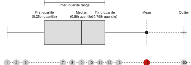
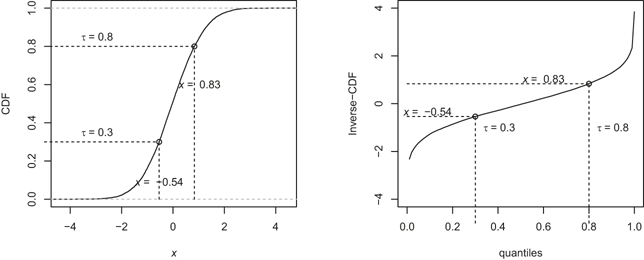
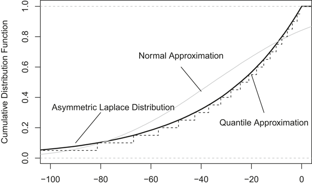
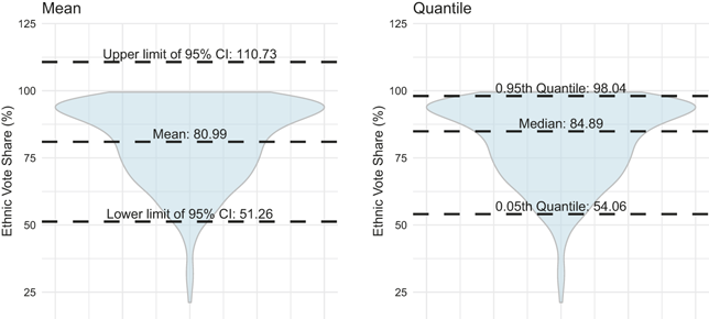
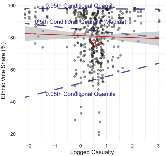
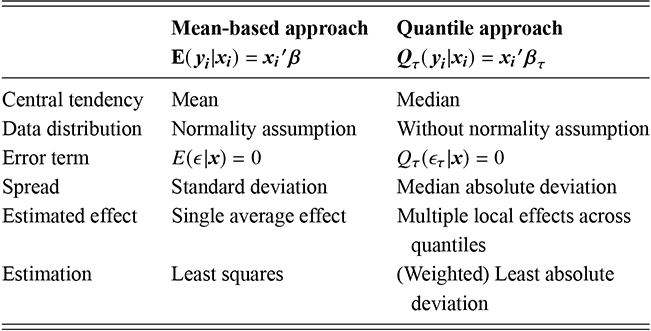
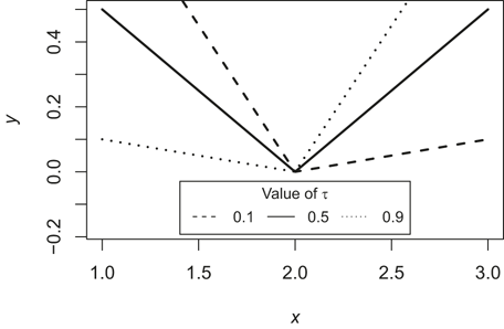

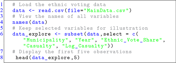
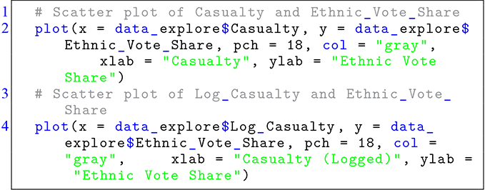
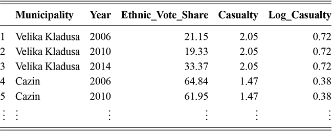
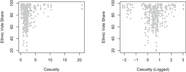
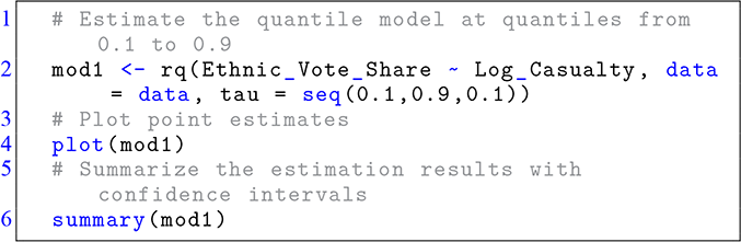
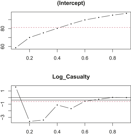
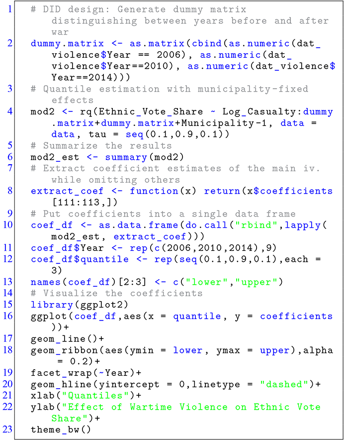
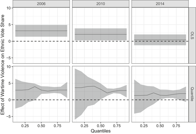
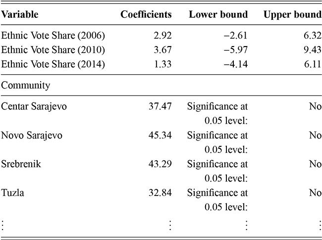
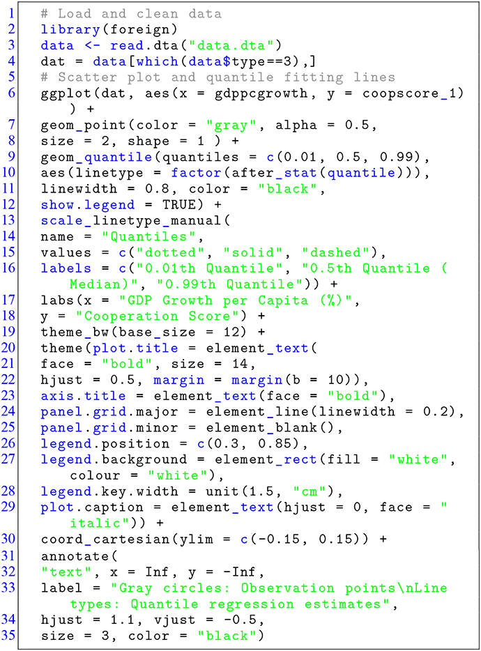
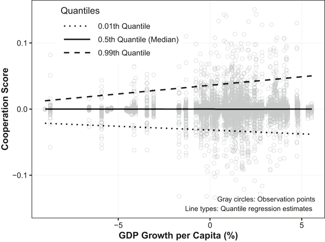
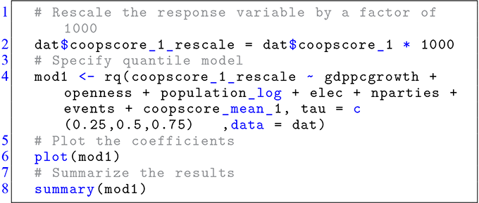
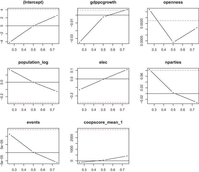
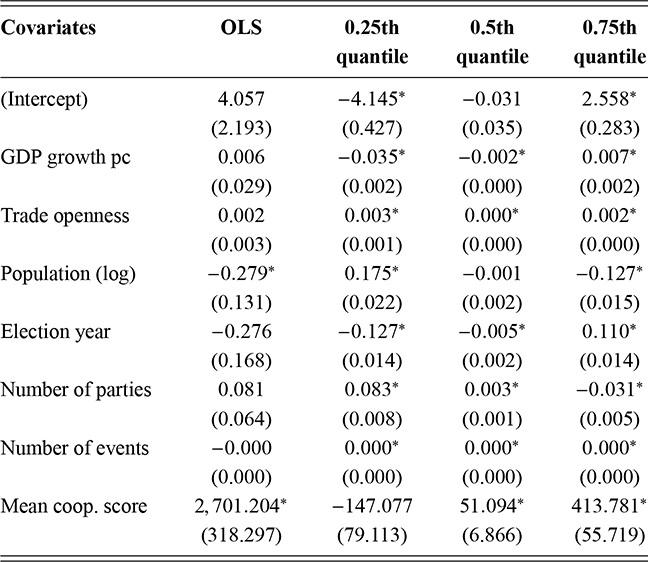
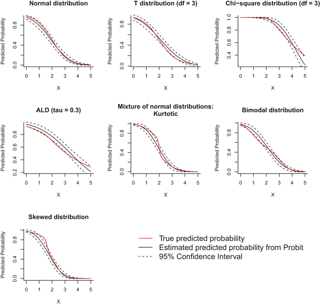
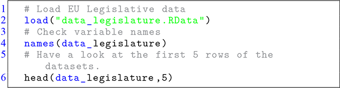
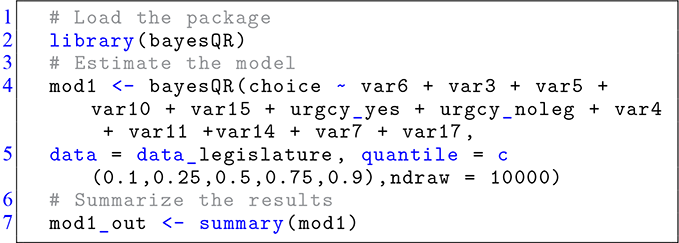

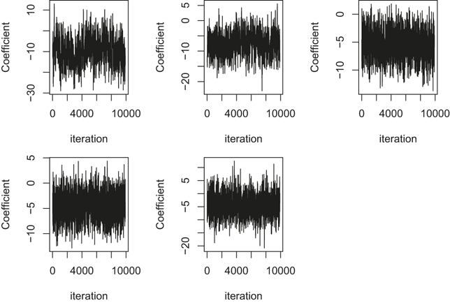
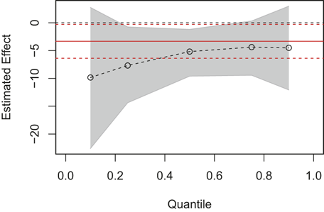

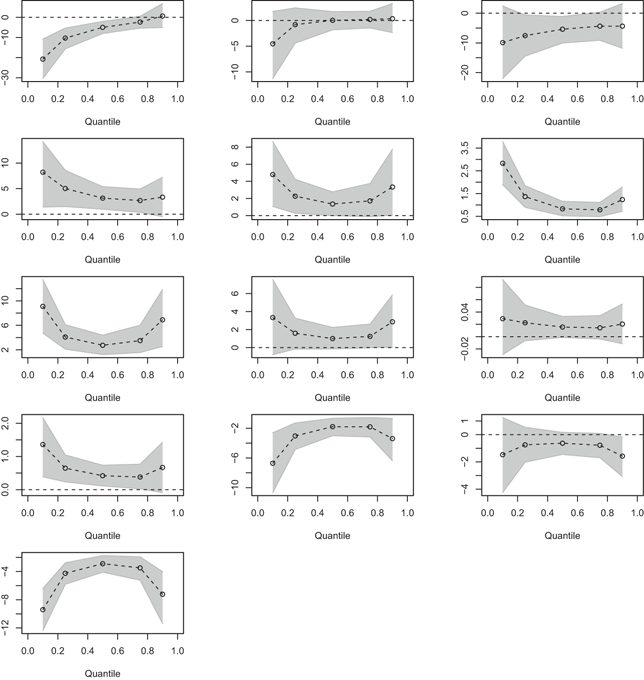

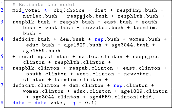
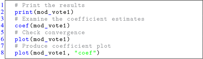
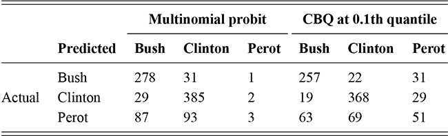
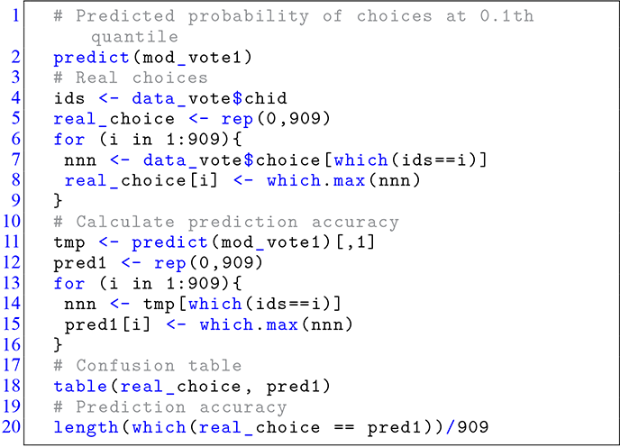
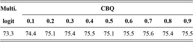
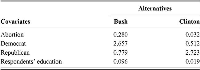

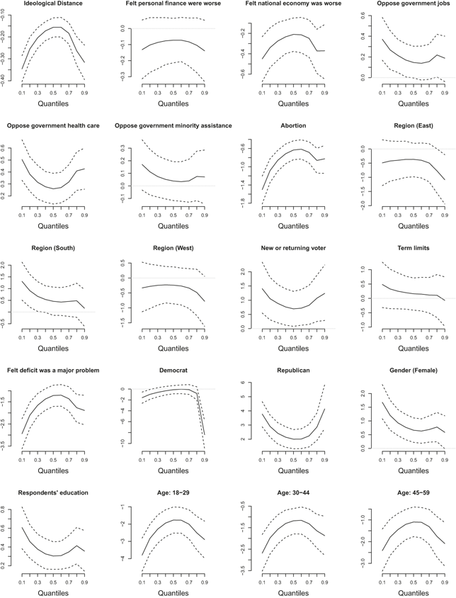
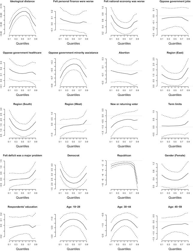
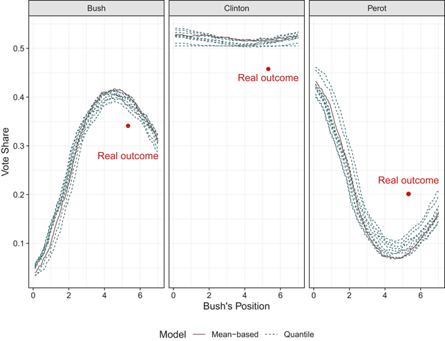
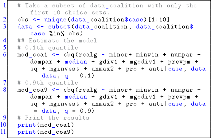
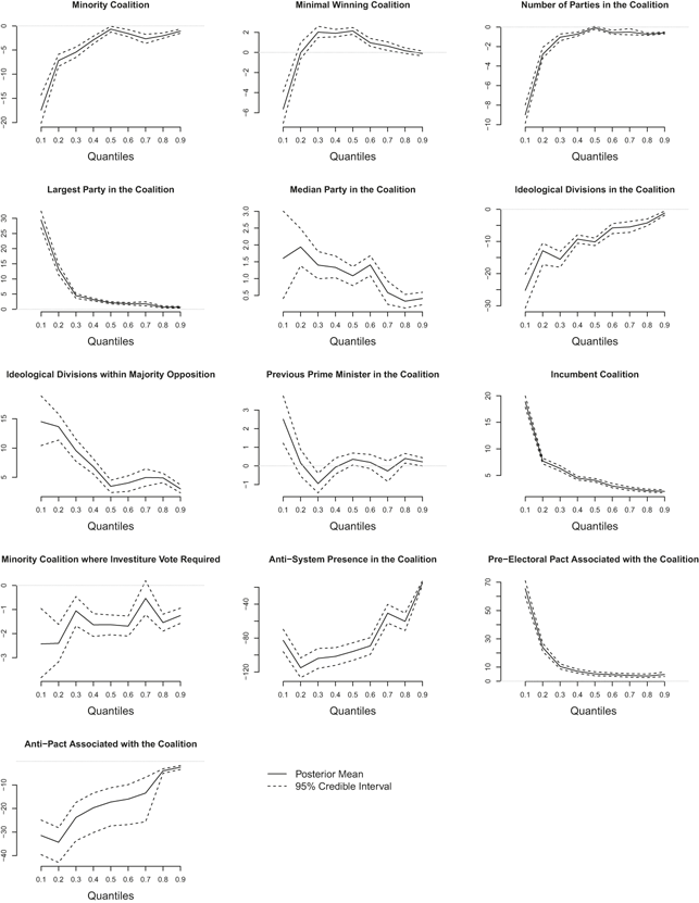
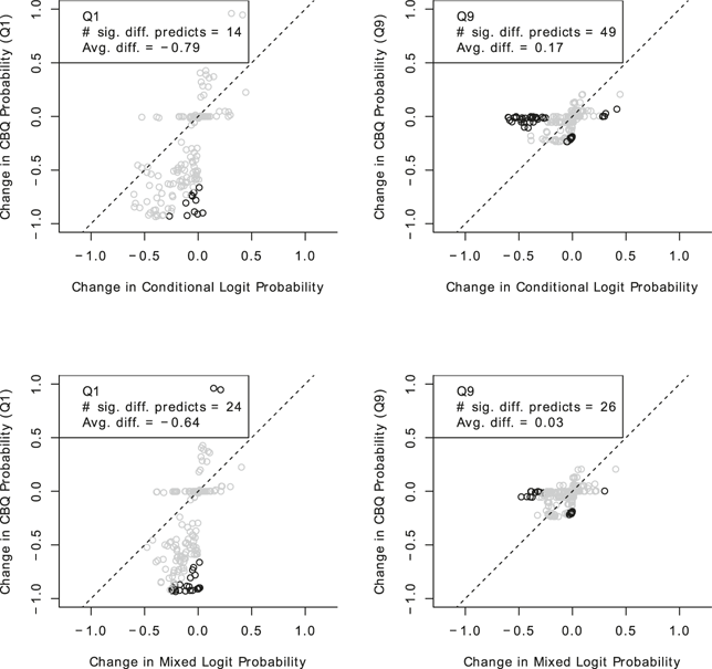
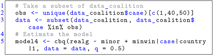
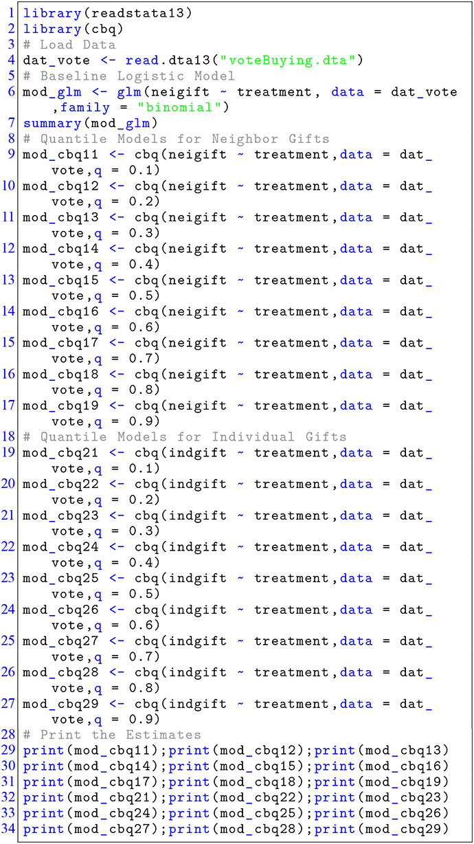
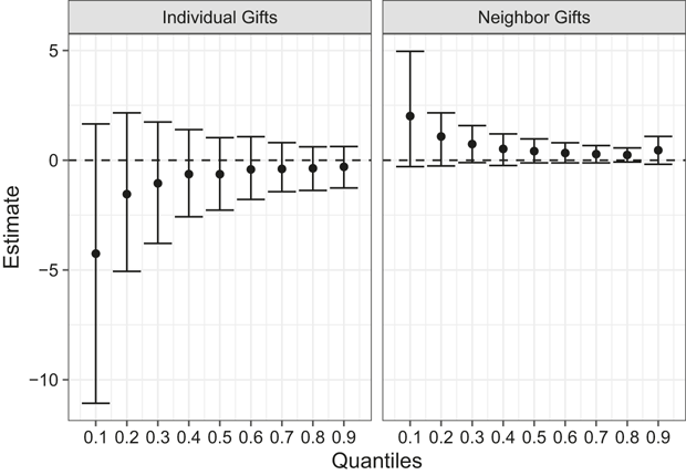
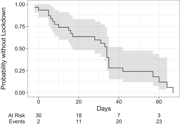
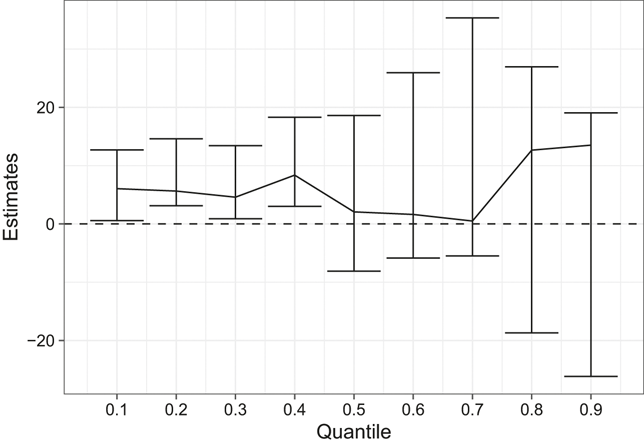
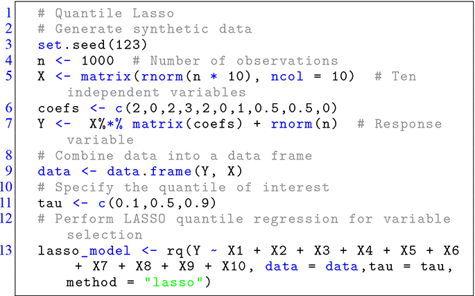
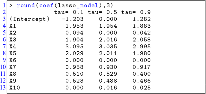
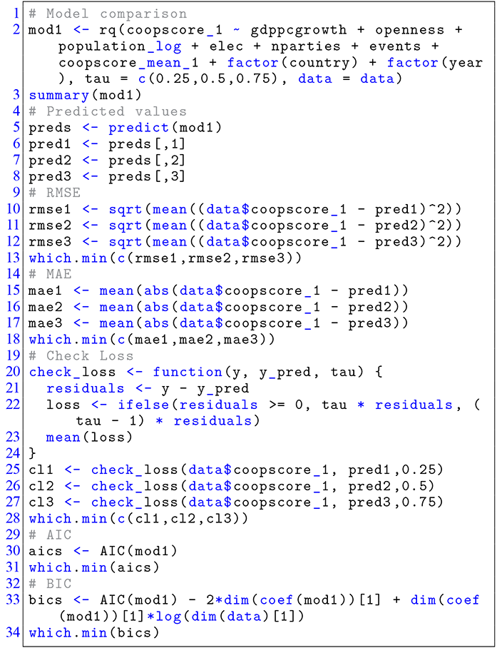

 Open access