


Impact statement
The asset-level Storm Water Management Model (SWMM)-calibrated Long Short-Term Memory (LSTM) surrogate model represents a major step forward in computational flood modeling, uniting the physical rigor of hydraulic simulations with the speed and predictive power of deep learning. This hybrid framework overcomes the computational limitations of traditional approaches without compromising accuracy, enabling real-time flood predictions that were previously infeasible. By providing rapid, reliable forecasts, the model empowers emergency responders, urban planners and infrastructure managers to perform swift scenario analyses during extreme weather events, informing decisions and enhancing public safety. As urban populations grow and climate change amplifies the frequency and intensity of extreme rainfall, the demand for resilient flood management systems becomes ever more urgent. This research offers a scalable, adaptable framework suitable for diverse urban environments, supporting the design of smart city infrastructure and promoting climate-resilient communities.
Introduction
In recent years, the frequency and intensity of extreme weather events have escalated, significantly affecting the socioeconomic development of communities (Idowu and Zhou, Reference Idowu and Zhou2023). Among these hazards, urban flooding is especially pervasive, damaging property, disrupting essential services and impeding residents’ daily mobility and communication (Samadi et al., Reference Samadi, Fowler, Lamond, Wagener, Brunner, Gourley, Moradkhani, Popescu, Wasko and Wright2025). Urban flooding events are often exacerbated by anthropogenic factors such as inadequate land-use planning, extensive impervious surface coverage, steep topography and stormwater drainage issues, including insufficient capacity, aging facilities and blockages in existing infrastructure.
To mitigate urban flooding impacts, a range of strategies have been developed, including practical management approaches such as nature-based solutions (e.g., green infrastructure; Guido et al., Reference Guido, Popescu, Samadi and Bhattacharya2023; Zafarmomen et al., Reference Zafarmomen, Samadi and Lunt2025a) and infrastructure upgrades aimed at directly reducing flood risk. Preceding these interventions, modeling approaches provide critical tools for simulating flood dynamics (e.g., real-time simulations), identifying vulnerabilities, mapping inundation extents and informing targeted interventions. In data-scarce or ungauged basins, digital elevation model-based approaches have also been successfully applied to delineate flood-prone areas and rapidly estimate inundation depth using primarily topographic information (Samela et al., Reference Samela, Manfreda, De Paola, Giugni, Sole and Fiorentino2016; Manfreda and Samela, Reference Manfreda and Samela2019). Recent work demonstrates that large language models can aid in the interpretation of extreme events, such as flooding, and deliver earlier alerts to communities (Zafarmomen and Samadi, Reference Zafarmomen and Samadi2025).
Urban hydrologic and hydraulic models serve as essential tools for planning, designing and managing water cycles in drainage systems (Sytsma et al., Reference Sytsma, Crompton, Panos, Thompson and Mathias Kondolf2022; Aderyani et al., Reference Aderyani, Jafarzadegan and Moradkhani2025; Zafarmomen et al., Reference Zafarmomen, Samadi and Borgomeo2025b). Fully distributed models, such as MIKE SHE (Abbott et al., Reference Abbott, Bathurst, Cunge, O’Connell and Rasmussen1986), LISFLOOD-FP (Bates and De Roo, Reference Bates and De Roo2000), MIKE FLOOD (Patro et al., Reference Patro, Chatterjee, Mohanty, Singh and Raghuwanshi2009) and InfoWorks ICM (Sidek et al., Reference Sidek, Jaafar, Majid, Basri, Marufuzzaman, Fared and Moon2021), solve complex differential equations like the Saint-Venant equations to capture flow dynamics across heterogeneous urban landscapes. By discretizing urban areas into computational grids, these models simulate surface runoff, channel flow and inundation patterns with high spatial precision. Their accuracy, however, depends heavily on detailed boundary conditions, including water surface elevation, inflows and outflows and bathymetric data.
Semi-distributed models, such as Storm Water Management Model (SWMM), Hydrologic Engineering Center Hydrologic Modeling System and MOUSE (DHI, 2017), strike a middle ground in complexity (Bennett, Reference Bennett1998; Rossman and Supply, Reference Rossman and Supply2006; Gironás et al., Reference Gironás, Roesner, Rossman and Davis2010). These models divide the urban catchment into sub-catchments and use conceptual or simplified physical methods to transform rainfall into hydrographs, which are then routed through a simplified drainage network. While less computationally demanding than fully distributed models, they capture the essential processes of flood generation and routing. At the simplest level, lumped approaches, such as the rational method or the Soil Conservation Service (SCS) Curve Number method (Paudel et al., Reference Paudel, Nelson and Scharffenberg2009), provide rapid estimates of peak discharge and runoff volume, often used in data-scarce contexts or preliminary planning. Overall, semi-distributed models balance the realism of fully distributed methods with the efficiency of lumped ones, making them widely applicable in urban flood risk management.
Recent research has increasingly focused on hybrid approaches that combine physics-based models with computational frameworks to improve predictive accuracy. Similar improvements in predictive skill have been reported in engineering applications using Artificial Neural Network (ANN) models (Mousavi et al., Reference Mousavi, Bengar, Mousavi, Mahdavinia and Bengar2025). For instance, Khatooni et al. (Reference Khatooni, Hooshyaripor, MalekMohammadi and Noori2025) coupled SWMM with Hydrologic Engineering Center’s River Analysis System Two-Dimensional (HEC-RAS-2D) to capture hydrologic–hydrodynamic interactions, while Wang et al. (Reference Wang, Chen, Zeng, Chen, Li, Jiang and Lai2024) developed the Storm Tide Unit Flood Modeling System (STUFMS), linking SWMM with the Télémac-2D Hydrodynamic Modeling System (TELEMAC-2D) for bidirectional water exchange. These frameworks improved predictions of flood depth and velocity, underscoring the value of hybrid systems for resilience planning. Similarly, Zhao et al. (Reference Zhao, Huo, Liu, Yang, Luo, Ahmed and Elbeltagi2024) combined SWMM with LISFLOOD to evaluate the joint effects of extreme rainfall and urbanization on inundation dynamics, and Li et al. (Reference Li, Yuan, Hu, Xu, Cheng, Song, Zhang, Zhu, Shang, Liu and Liu2024) applied LISFLOOD to simulate spatiotemporal flood evolution and assess its impact on population, land use and buildings.
Hydrological modeling has advanced significantly through improved physical models, data assimilation techniques and machine learning (ML) methods (Zafarmomen et al., Reference Zafarmomen, Alizadeh, Bayat, Ehtiat and Moradkhani2024). Building on these developments, ML and deep learning (DL) have become promising tools that complement traditional physics-based approaches. By leveraging large datasets, ML/DL models improve predictive accuracy and timeliness (Javadi et al., Reference Javadi, Jalilehvand, Alizadeh and Zafarmomen2025), enabling integration with hydrologic and hydraulic models. For example, Zhao et al. (Reference Zhao, Liu, Li, Tang, Yang, Xu, Quan and Hu2023) coupled Long Short-Term Memory (LSTM) with SWMM to enhance runoff predictions at outlet points, while Shao et al. (Reference Shao, Chen, Zhang, Yu and Chu2024) introduced CRU-Net, a recurrent U-shaped network capable of predicting inundation areas at speeds far surpassing LISFLOOD-FP. More recently, Pan et al. (Reference Pan, Hou, Gao, Chen, Li, Imran, Li, Yang, Ma and Zhou2025) proposed a coupled SWMM–LSTM framework that incorporates sewer network outputs into surface flood modeling, demonstrating strong performance in predicting node overflow, inundation depth and flooded area.
While these studies advanced LSTM–hydrodynamic coupling, they primarily focused on either grid-based inundation or outlet-level performance. In contrast, this study develops a spatiotemporal LSTM surrogate trained on SWMM outputs to predict event-level maximum water depth and inflow at the node scale. By explicitly integrating hydrologic conditions and network connectivity, the model identifies hydraulic hotspots through inter-event variability, enabling rapid and scalable real-time flood forecasting. The framework captures rainfall–runoff dynamics by combining spatial dependencies across the drainage network with temporal storm variability, delivering robust node-level predictions of (i) maximum water depth (m) and (ii) maximum inflow (m3/s). By reducing computational costs while maintaining high predictive accuracy, this surrogate model offers a practical alternative to traditional hydrologic–hydraulic approaches for operational flood management.
This paper is structured as follows: Section “Methodology” describes the case study, SWMM setup and surrogate model development, including hyperparameter tuning and evaluation outcomes and predictive skill across various average recurrence intervals (ARIs). Section “Discussion and conclusion” discusses conclusions, highlighting the effectiveness of the spatiotemporal LSTM surrogate, its implications for urban flood management and avenues for future research.
Methodology
Case study
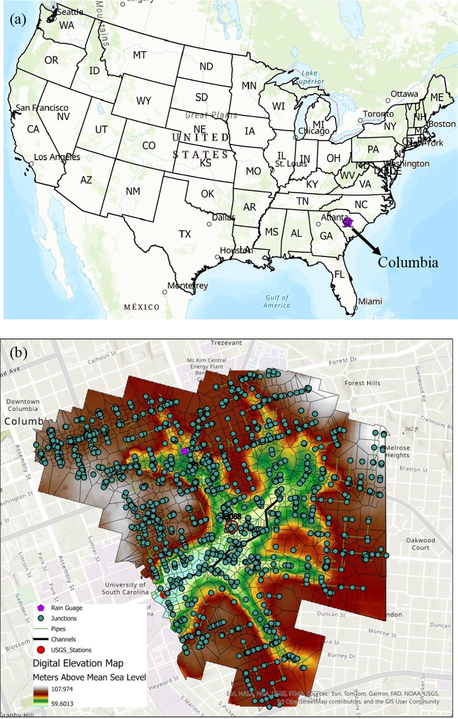
The Rocky Branch Watershed, a sub-watershed of the Congaree River located in Columbia, South Carolina, USA, is highly susceptible to urban flooding due to its unique topographic and anthropogenic characteristics. The watershed is characterized by steep slopes and a dense storm drainage network, which, combined with extensive urbanization, significantly exacerbates flood risks. Urban development has led to a predominance of impervious surfaces and substantial land-use changes, resulting in reduced infiltration rates, particularly within the central business district (Hung et al., Reference Hung, James, Carbone and Williams2020). Ress et al. (Reference Ress, Hung and James2020) demonstrate a strong correlation between runoff coefficients and the percentage of impervious areas, highlighting the critical role of urban land cover in amplifying surface runoff. Despite these challenges, conventional stormwater management measures in the Rocky Branch Watershed remain limited, contributing to persistent flash flooding issues that pose ongoing threats to infrastructure and public safety.
The spatial distribution of flood risk within the watershed is shown in the USGS elevation map (Figure 1), which illustrates the topographic variability and infrastructure layout. The map highlights steep elevation gradients, particularly in the central and eastern portions of the watershed, where dense clusters of rain gauges and pipes indicate a complex drainage system. These areas, encompassing key urban zones such as the University of South Carolina main campus and surrounding neighborhoods, exhibit heightened vulnerability due to the convergence of steep slopes and impervious surfaces. The green and yellow zones on the map signify lower elevations prone to water accumulation, while the red and brown areas denote higher elevations that accelerate runoff toward low-lying regions.
(a) Location of Columbia in South Carolina, USA. (b) Spatial configuration of the stormwater network and topography in the Rocky Branch Watershed, Columbia, South Carolina.

Drainage simulation model
The US EPA’s SWMM is a dynamic hydrologic–hydraulic simulator widely adopted for urban drainage analysis (Rossman, Reference Rossman2010). It couples rainfall–runoff generation with flow routing and water-quality processes across sewer networks (Rossman and Huber, Reference Rossman and Huber2016). Urban domains are partitioned into subcatchments connected by nodes and links (e.g., manholes, conduits and channels), enabling simulation of surface runoff and conveyance through pipe systems. Runoff production is represented by a nonlinear reservoir formulation, and the platform supports both event-based and continuous simulations for design, planning and operations (Huber et al., Reference Huber, Dickinson, Barnwell and Branch1988).
In this study, we apply SWMM to a 10.75-km2 watershed comprising 2,802 manholes and 2,801 conduits spanning 17.02 km. The watershed was subdivided into multiple drainage catchments using the Thiessen polygon method, which allocates contributing areas to junction nodes based on proximity. This approach is widely used in urban hydrologic modeling to define subcatchments in the absence of high-resolution flow routing data (Dong et al., Reference Dong, Bain, Akcakaya and Ng2023). Conduit diameters range from 8 to 84 inches and include 14 material types; reported Manning’s roughness values span 0.009 for polyethylene to 0.027 for corrugated metal. Field-surveyed elevations, maximum depths and inlet/outlet offsets are incorporated to reflect as-built conditions (Table 1). This high-resolution network and material heterogeneity provide a robust basis for hydraulic performance assessment, calibration and sensitivity analysis and scenario testing under extreme rainfall, supporting reliable urban flood risk evaluation and system planning.
Summary of Rocky Branch stormwater drainage network characteristics

The graphical user interface for SWMM was originally developed and maintained by the US EPA. In our study, the PySWMM Python library, developed by McDonnell et al. (Reference McDonnell, Ratliff, Tryby, Wu and Mullapudi2020), served as a Python wrapper for the SWMM engine, enabling full execution and fine-grained control of dynamic simulations directly within the Python environment. This integration enables advanced workflows by providing a seamless pathway for implementing ML/DL techniques, thereby strengthening automation, calibration procedures and real-time modeling applications.
This study utilizes the Saint-Venant equations to simulate unsteady water flow within a drainage network through pipes and channels. The governing equations include the continuity equation for mass conservation (Equation 1) and the momentum equation (Equation 2), respectively (Lai, Reference Lai1986). SWMM employs the full version of these equations to model free surface flow dynamics.
 $$ \frac{\partial A}{\partial t}+\frac{\partial Q}{\partial x}=0 $$
The term $ \frac{\partial A}{\partial t} $
represents the rate of change of the cross-sectional flow area A with respect to time t, accounting for the temporal variation in water storage. Moreover,
$ \frac{\partial A}{\partial t} $
represents the rate of change of the cross-sectional flow area A with respect to time t, accounting for the temporal variation in water storage. Moreover, $ \frac{\partial Q}{\partial x} $
represents the spatial gradient of the discharge Q along the flow direction x, describing the change in flow rate along the channel or pipe.
$ \frac{\partial Q}{\partial x} $
represents the spatial gradient of the discharge Q along the flow direction x, describing the change in flow rate along the channel or pipe.
 $$ \frac{\partial Q}{\partial t}+\frac{\partial \left({Q}^2/A\right)}{\partial x}+ gA\frac{\partial H}{\partial x}+ gA{S}_f+ gA{h}_L=0 $$
where $ A $
is the cross-sectional area,
$ A $
is the cross-sectional area, $ Q $
is the flow rate,
$ Q $
is the flow rate, $ {S}_f $
represents the friction slope and
$ {S}_f $
represents the friction slope and $ {h}_L $
accounts for energy losses caused by local hydraulic features, such as bends, expansions, contractions or other structures. Additionally,
$ {h}_L $
accounts for energy losses caused by local hydraulic features, such as bends, expansions, contractions or other structures. Additionally, $ H $
denotes the water surface elevation. It is worth noting that the area
$ H $
denotes the water surface elevation. It is worth noting that the area $ A $
is a known function of flow depth
$ A $
is a known function of flow depth $ y $
, which in turn can be derived from the head H.
$ y $
, which in turn can be derived from the head H.
This study employs the Horton infiltration model by applying the classical exponential decay function to simulate surface infiltration (Equation 3).
 $$ f(t)={f}_{\infty }+\left({f}_0-{f}_{\infty}\right){e}^{-\alpha t} $$
where $ {f}_0 $
is the initial infiltration rate,
$ {f}_0 $
is the initial infiltration rate, $ {f}_{\infty } $
is the minimum (asymptotic) infiltration rate after long wetting and
$ {f}_{\infty } $
is the minimum (asymptotic) infiltration rate after long wetting and $ \alpha $
is the decay coefficient representing how quickly infiltration decreases.
$ \alpha $
is the decay coefficient representing how quickly infiltration decreases.
Cumulative infiltration is updated at each time step as:
 $$ F\left(t+\Delta t\right)=F(t)+\hat{f}\Delta t $$
where F(t) is the cumulative infiltration at time t, and $ \hat{f} $
is the average infiltration rate during the time step. Moreover, Infiltration recovers during dry periods, ensuring accurate modeling of variable antecedent conditions.
$ \hat{f} $
is the average infiltration rate during the time step. Moreover, Infiltration recovers during dry periods, ensuring accurate modeling of variable antecedent conditions.
 $$ {f}_P={f}_{\infty }+\left({f}_0-{f}_{\infty}\right)\;{e}^{-{k}_d\left(t-{t}_w\right)} $$
where $ {f}_P $
is the regenerated infiltration capacity at time t,
$ {f}_P $
is the regenerated infiltration capacity at time t, $ {k}_d $
is the attenuation coefficient for the recovery curve and
$ {k}_d $
is the attenuation coefficient for the recovery curve and $ {t}_w $
is the hypothetical time when recovery started.
$ {t}_w $
is the hypothetical time when recovery started.
Moreover, the hydraulic simulation of the drainage system’s pipe network is conducted using the dynamic wave method, while the underlying principles of the model are formulated as follows
 $$ {R}_s={\int}_{i>{f}_p}\left(i-{f}_p\right) dt $$
where Rs is surface runoff (mm), i is the rainfall intensity (mm/h).
Prior work in the Rocky Branch Watershed by Tanim et al. (Reference Tanim, Smith-Lewis, Downey, Imran and Goharian2024) and Morsy et al. (Reference Morsy, Goodall, Shatnawi and Meadows2016) applied SWMM with sub-catchment outlets positioned at fixed 50-m intervals. In contrast, we explicitly represent the drainage system at the asset level (manholes, pipes and inlets) using surveyed elevations and offsets, thereby achieving higher hydraulic resolution. Because a hydrologic–hydraulic model requires calibration, we treated the parameter ranges reported in those studies (e.g., imperviousness, Manning’s n value and Horton infiltration parameters) as priors and refined them via targeted trial-and-error. Calibration focused on reproducing the observed hydrograph at the USGS gauging station 02169505 on Rocky Branch, with emphasis on peak magnitude and timing. Rainfall data for these events were obtained from the nearby USGS gauge 021695045. Final parameter sets were selected to maximize the evaluation criteria.
The model was calibrated using two distinct storm events from the 2015–2024 USGS record, selected for their hydroclimatic diversity. The event of 13–14 December 2019 was a long-duration winter frontal storm (99.3 mm over 29.25 h), while the 25 July 2024 event was a short-duration summer convective storm (13.5 mm over 1.25 h). Both events ranked in the top 10% of intensity for the period, ensuring the calibration captured a wide range of hydrologic responses.
DL model
LSTM
The LSTM unit uses three gates: input, forget and output, to regulate how information enters, is retained, and is revealed from a long-term cell state. This design preserves long-range temporal dependencies while updating a hidden state that reflects recent information, making LSTMs well-suited to rainfall–runoff sequences. At each time step, the gates (sigmoid activations) and a tanh-based proposed update adjust the cell state and produce the hidden state, enabling stable learning without vanishing gradients (Hochreiter and Schmidhuber, Reference Hochreiter and Schmidhuber1997). LSTMs have shown promising improvement in forecasting flood-related time series, accurately modeling complex rainfall–runoff relationships (Saberian et al., Reference Saberian, Samadi and Popescu2024; Saberian et al., Reference Saberian, Zafarmomen, Panthi and Samadi2026).
In this study, the LSTM receives time-varying rainfall and related predictors and predicts event-level maxima (water depth and inflow). Full gate equations and training details are provided in the Supplementary Material (Supplementary Equations 1–5).
To train the DL model, we generated a dataset of 5,000 synthetic design hyetographs. These synthetic hyetographs were generated using a statistically based design storm method grounded in National Oceanic and Atmospheric Administration Atlas 14 precipitation frequency estimates. For each of the seven ARIs (1, 2, 5, 10, 25, 50 and 100 years), event total depths were distributed sampled from the 90% confidence intervals of Atlas 14 across 10 storm durations (5, 10, 15 and 30 min; 1, 2, 3, 6, 12 and 24 h) as provided in Supplementary Table S1, to account for variability. The temporal distribution within each storm was synthesized using a stochastic approach based on Huff’s quartile curves (Huff, Reference Huff1967), with sampling weights of 0.40 (first quartile), 0.25 (second), 0.20 (third) and 0.15 (fourth) to ensure diversity in storm patterns (Yin et al., Reference Yin, Xie, Nearing, Guo and Zhu2016). This was further perturbed with Dirichlet noise (Anello and Cordaro, Reference Anello and Cordaro2007) to create variability in peak timing and intensity while strictly conserving the total depth. All hyetographs were generated at a 15-min resolution and assumed to be spatially uniform across the watershed, a reasonable simplification for its scale (i.e., 10.75 km2), consistent with prior local studies (Morsy et al., Reference Morsy, Goodall, Shatnawi and Meadows2016; Tanim et al., Reference Tanim, Smith-Lewis, Downey, Imran and Goharian2024). For each event, the input sequence Ut comprises rainfall intensity through time, and the network predicts, for every drainage node, the event-level maxima: (i) maximum water depth (m) and (ii) maximum inflow (m3/s). From a hydrologic perspective, maximum water depth characterizes the storage response within local depressions or manholes, reflecting the balance of inflow, conveyance and infiltration at the point scale, while maximum inflow represents the cumulative runoff contributions from upstream subcatchments, capturing the rainfall–runoff transformation over the drainage area. Maximum water depth is a critical indicator of localized flood hazard, directly linked to surface inundation and infrastructure exposure, while maximum inflow reflects the integrated upstream hydrologic response that governs conveyance capacity and potential surcharging within the drainage network. Targets are obtained from the calibrated hydrologic–hydraulic model. An LSTM architecture is adopted because it captures long-range temporal dependencies and nonlinear threshold responses inherent to rainfall–runoff transformation and hydraulic routing, enabling accurate, computationally efficient node-level forecasts. This configuration is designed to enhance both offline and real-time flood prediction capabilities in urban drainage networks. The framework maps rainfall sequences to event-level maxima of water depth and inflow. In offline mode, the framework functions as a high-speed emulator of the SWMM, enabling rapid vulnerability assessments. In real-time mode, the model can be driven through real-time rainfall data to deliver continuously updated forecasts of maximum hydraulic responses during ongoing storm events. The LSTM dynamically encodes cumulative rainfall through its memory state to represent hydrologic dependencies and storage evolution. As new observations become available, predictions are incrementally refined, supporting near-real-time, node-level flood risk assessment and enabling proactive urban flood management.
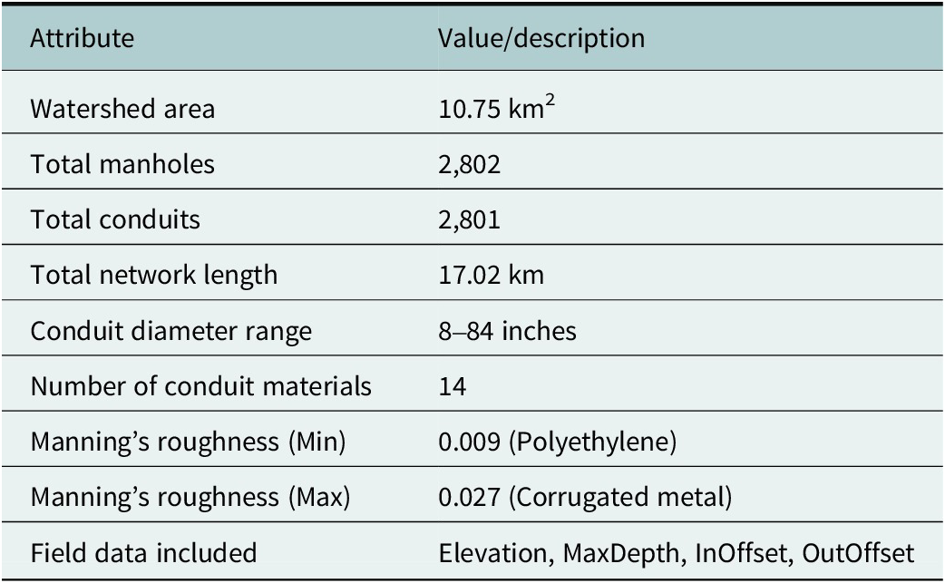
Figure 2 illustrates the hybrid workflow. SWMM generates node-level targets from rainfall events, which are then used to train an LSTM that maps predictor sequences to maximum water depth and inflow for real-time prediction.
SWMM–LSTM workflow for surrogate modeling. (a) SWMM process: rainfall is processed through infiltration, surface runoff, and dynamic-wave routing to produce node-level maxima (water depth and inflow), which are used as training targets; (b) Repository of event datasets containing rainfall time series and the corresponding SWMM targets; (c) Input sequence: r time steps by c predictors assembled per node event; and (d) to predict node-level depth and inflow in real time, while SWMM is used only offline to generate training labels.

Hyperparameter tuning
The optimal configuration of hyperparameters was identified through a Grid Search methodology, a systematic and exhaustive approach that explores a comprehensive search space encompassing critical parameters of LSTM, such as the number of hidden units, the number of layers and dropout rates. This strategy evaluates every possible combination of these hyperparameters, rendering it an effective technique when the parameter set and their respective value ranges remain computationally tractable. Nevertheless, the method’s computational demands increase significantly with an expanding search space, posing challenges particularly when training sophisticated DL architectures.
Prior to hyperparameter tuning, the dataset of 5,000 events was partitioned into training (70%), validation (15%) and test (15%) subsets. The split was performed in a stratified manner based on the annual recurrence interval (ARI) categories to ensure a balanced representation of storm intensities across all subsets. The training set was used for model learning, the validation set for guiding the hyperparameter optimization and early stopping and the held-out test set was reserved for the final performance evaluation reported in Section “Results.”
The architectural framework of the model featured an LSTM network, configured with a range of hidden units (16–256), layer depths (1–4) and dropout rates (0–0.4). Each model instantiation was optimized using the Adam optimizer, set with a learning rate of 0.001 to ensure convergence.
The rectified linear unit activation function was implemented within the hidden LSTM layers to introduce nonlinearity and mitigate vanishing gradient issues, while a linear activation function was adopted at the output layer.
Evaluation criteria
The predictive accuracy and robustness of both the calibrated hydrologic–hydraulic model and the LSTM-based surrogate models were assessed using statistical performance metrics. These criteria quantify different aspects of model performance, including overall goodness of fit, error magnitude and bias, and are particularly relevant for maximum water depth and maximum inflow across the drainage network nodes.
The Nash-Sutcliffe Efficiency (NSE) is a dimensionless metric that quantifies the predictive accuracy of the model by comparing the variance of the residuals to the variance of the observed data (Nash and Sutcliffe, Reference Nash and Sutcliffe1970).
 $$ NSE=1-\frac{\sum_{i=1}^n{\left({Q}_{obs,i}-{Q}_{sim,i}\right)}^2}{\sum_{i=1}^n{\left({Q}_{obs,i}-\overline{Q_{obs}}\right)}^2} $$
where Qobs and Qsim are the observed and simulated values at time step i, respectively, $ \overline{Q_{\mathrm{obs}}} $
is the mean of the observed values and n is the number of observations.
$ \overline{Q_{\mathrm{obs}}} $
is the mean of the observed values and n is the number of observations.
The root mean square error measures the average magnitude of the prediction errors in the same units as the target variable (Chai and Draxler, Reference Chai and Draxler2014). It emphasizes larger errors due to the squaring of residuals.
 $$ RMSE=\sqrt{\frac{\sum_{i=1}^n{\left({Q}_{obs,i}-{Q}_{sim,i}\right)}^2}{n}} $$
The mean absolute error (MAE) provides a measure of the average absolute difference between observed and simulated values (Willmott and Matsuura, Reference Willmott and Matsuura2005).
 $$ MAE=\frac{\sum_{i=1}^n\left|{Q}_{obs,i}-{Q}_{sim,i}\right|}{n} $$
To evaluate the storm-to-storm variability at each node, independent of the absolute magnitude of the maxima, we compute a normalized row-wise standard deviation across events. Let $ \left\{{x}_{j1},{x}_{j2},\dots, {x}_{jm}\right\} $
denote the event-wise maxima at node j, where m represents the total number of events (Han et al., Reference Han, Kamber and Mining2006). A 0–1 normalization is first applied within node j to standardize the data. The normalized value
$ \left\{{x}_{j1},{x}_{j2},\dots, {x}_{jm}\right\} $
denote the event-wise maxima at node j, where m represents the total number of events (Han et al., Reference Han, Kamber and Mining2006). A 0–1 normalization is first applied within node j to standardize the data. The normalized value $ \overset{\sim }{x_{jk}} $
for event k at node j is defined as:
$ \overset{\sim }{x_{jk}} $
for event k at node j is defined as:
 $$ \overset{\sim }{x_{jk}}=\left[\begin{array}{c}\frac{x_{jk}-{\mathit{\min}}_k{x}_{jk}}{{\mathit{\max}}_k{x}_{jk}-{\mathit{\min}}_k{x}_{jk}},\hskip0.6em {\mathit{\max}}_k{x}_{jk}>{\mathit{\min}}_k{x}_{jk}\\ {}0,\hskip0.48em otherwise\end{array}\right. $$
This normalization ensures that the values are scaled to the interval [0,1], preserving relative differences while removing the influence of absolute magnitude.
To quantify how sensitive each junction is to different storm configurations of the same statistical intensity, we define a normalized inter-event variability metric (Equation 10), calculated as the standard deviation of predicted maxima (water depth or inflow) across all events within each ARI class, normalized by the corresponding median. It effectively captures the fluctuation in flood severity due to differences in temporal rainfall structure, antecedent loading and internal hydraulic dynamics.
By combining these complementary evaluation metrics, the study ensured a rigorous assessment of model performance, capturing both general fit quality and the specific ability to reproduce critical flood characteristics relevant to urban flood risk management.
Results
Calibration performance
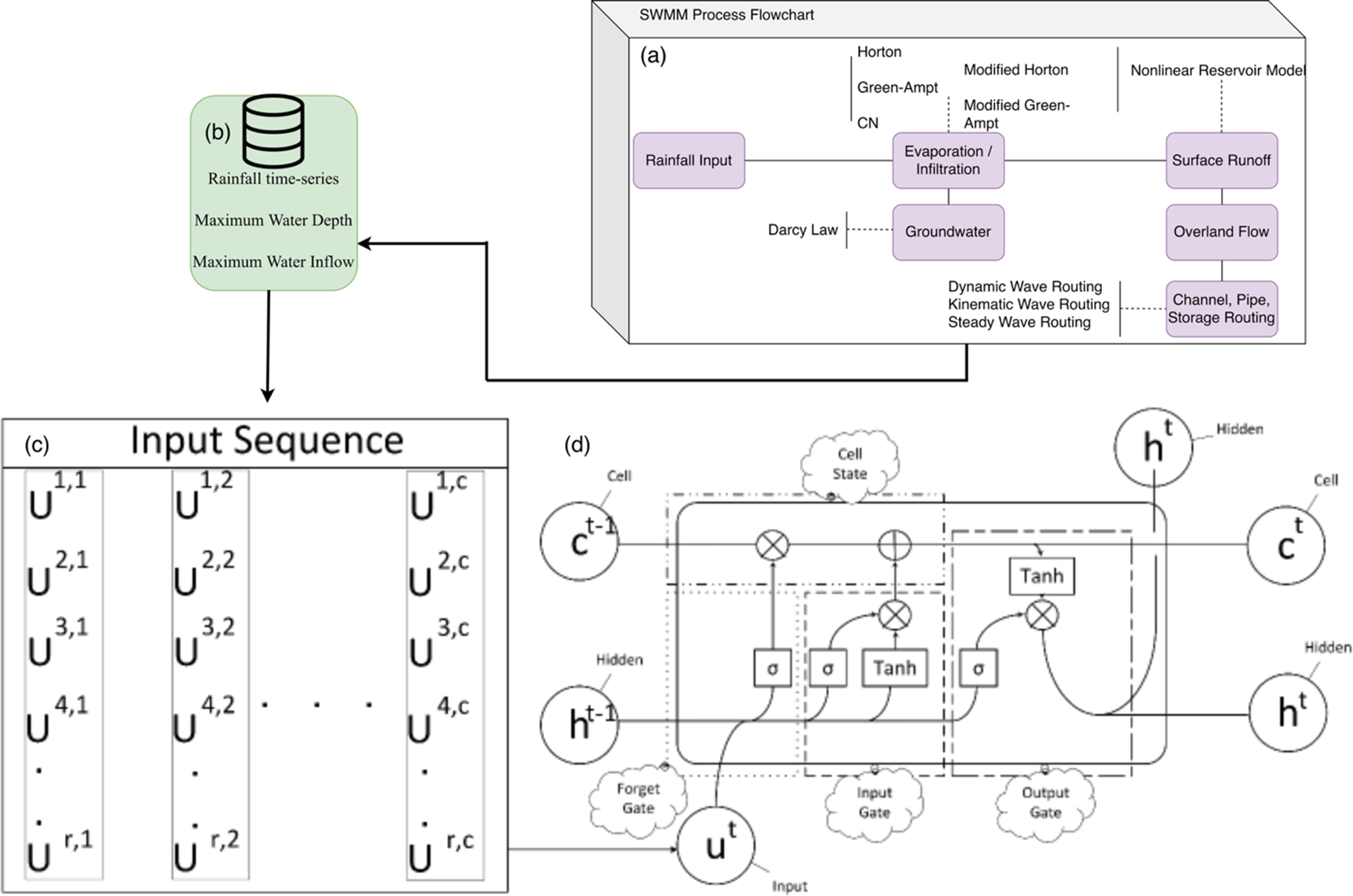
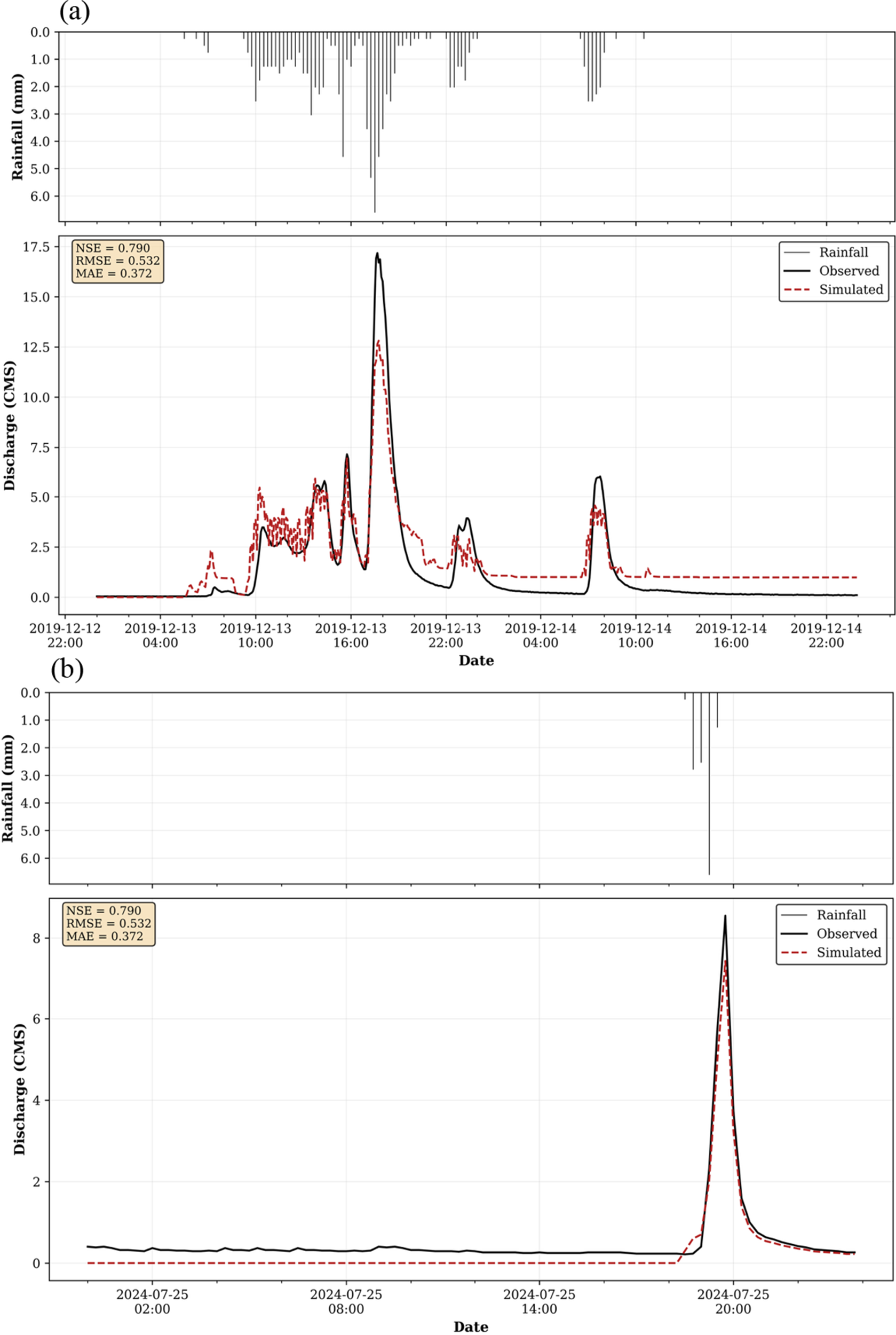
Figure 3 illustrates the calibration performance of the hydrology-hydraulic model, examined using two events spanning 13–14 December 2019 and 25 July 2024 within the Rocky Branch Watershed. Both the observed rainfall and USGS discharge data used for calibration were at a 15-min temporal resolution. The figure presents a time series comparison: rainfall is shown in the upper panel as an inverted hyetograph (mm), while the lower panel depicts the temporal variation of observed and simulated discharges (m3/s). The SWMM model performance during calibration was assessed using three widely adopted statistical indicators: NSE, RMSE and MAE. The calibrated model achieved NSE values of 0.790 and 0.820 for the two events, respectively, indicating a high degree of agreement between observed and simulated flows. Corresponding RMSE values were 0.532 and 0.496 m3/s, while MAE values were 0.372 and 0.357 m3/s, respectively. These results demonstrate the model’s capability to reproduce both the magnitude and timing of peak flows with minimal deviation from observations.
Time series comparison for (a) 13–14 December 2019 and (b) 25 July 2024, showing the rainfall hyetograph (mm) and observed versus simulated discharge hydrographs (Cubic Meters per Second (CMS)), representing the SWMM calibration events.

Visual hydrograph inspection demonstrated that the model effectively reproduced the rising and recession limbs of the flood events, along with the peak discharge magnitudes. Minor discrepancies were observed in the timing and magnitude of secondary peaks, likely stemming from uncertainties in rainfall distribution, spatial variability in infiltration and the simplification in the representation of drainage network features within the model. Moreover, the calibration extends to a winter and a summer storm, demonstrating that the model maintains comparable skill under different seasonal regimes and storm types. Nevertheless, the overall calibration performance indicated that the model was well-suited for simulating flood dynamics in the study area and provided a reliable foundation for subsequent scenario analysis.
Hyperparameter tuning
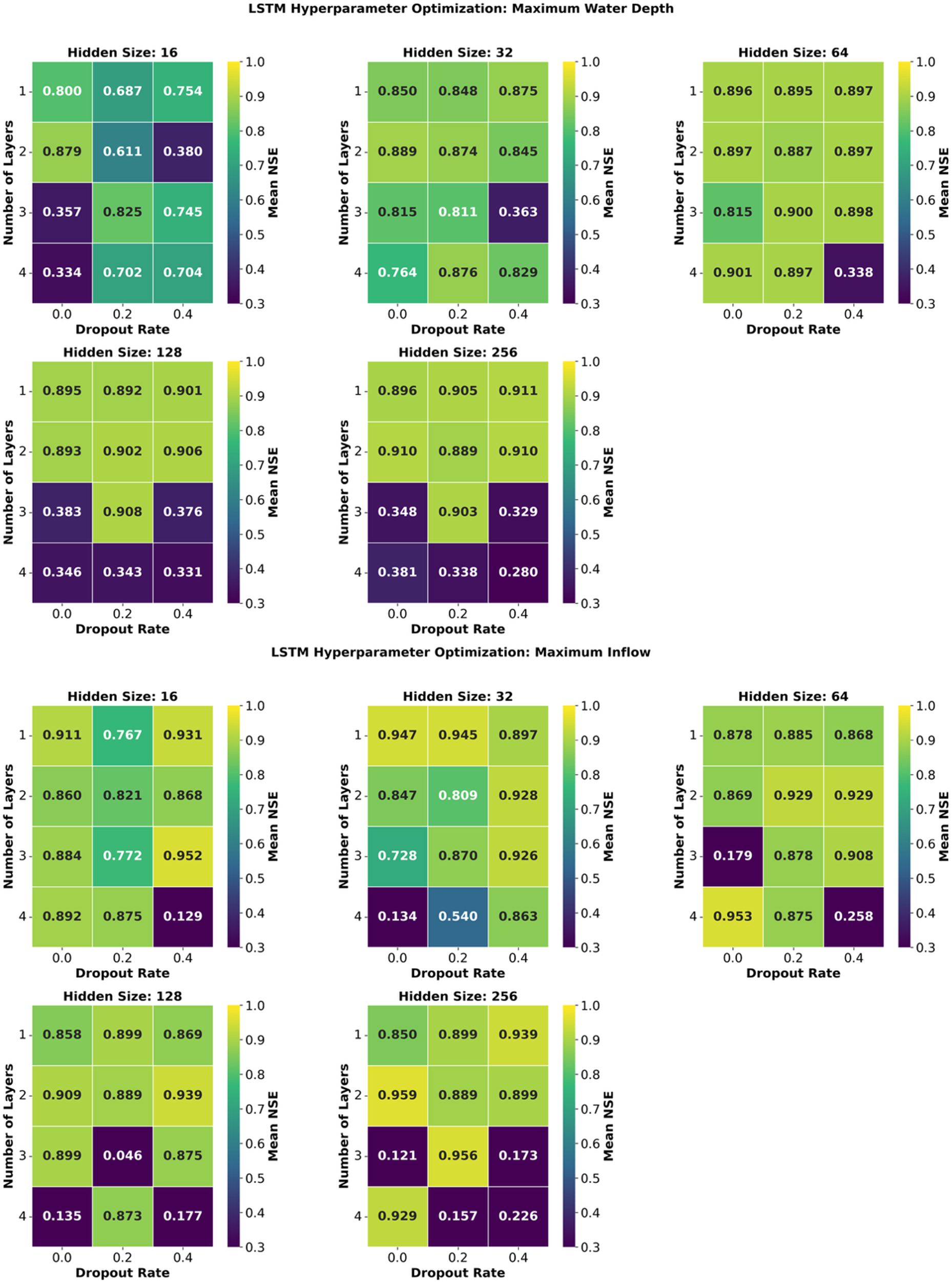
Figure 4 presents the mean NSE values for predicting maximum water depth and maximum inflow across different LSTM hyperparameter configurations. The maximum water depth trend suggested that a larger hidden size combined with moderate dropout enhanced model robustness and predictive accuracy, likely by mitigating overfitting while capturing complex patterns in the data. For maximum water depth prediction, the highest mean NSE value of 0.91 was achieved with a hidden size of 256, a single layer and a dropout rate of 0.4. Notably, smaller hidden sizes (e.g., 16) yielded lower mean NSE values (0.65), underscoring the importance of sufficient model capacity. In contrast, for maximum inflow prediction, the best NSE of 0.96 was observed with a hidden size of 256, two layers and no dropout. This suggested that a balance between network depth and minimal regularization was optimal for this task, potentially due to the inherent variability in inflow data requiring less aggressive dropout to retain critical features. Interestingly, maximum inflow prediction demonstrated higher peak NSE values than water depth prediction across all hidden sizes, indicating greater learnability for inflow patterns under optimal configurations. The mean NSE values across hidden sizes showed a decline with increasing size (e.g., 0.81 for size 16 vs. 0.67 for size 256), highlighting that smaller to moderate hidden sizes sufficed when paired with appropriate layering, as seen with the best configuration at hidden size 64 (mean NSE 0.78).
Heatmap comparison of mean NSE values for predicting maximum water depth (top panel) and maximum inflow (bottom panel) using various LSTM hyperparameter configurations, including hidden size, number of layers and dropout rate.

However, the optimal configuration varied slightly between water depth and inflow prediction, suggesting that the two tasks required fine-tuned architecture rather than a single shared optimal model. The results indicated that hyperparameter tuning was task-specific, with water depth predictions benefiting from larger hidden sizes and higher dropout rates, while inflow predictions favored moderate network depths with minimal dropout.
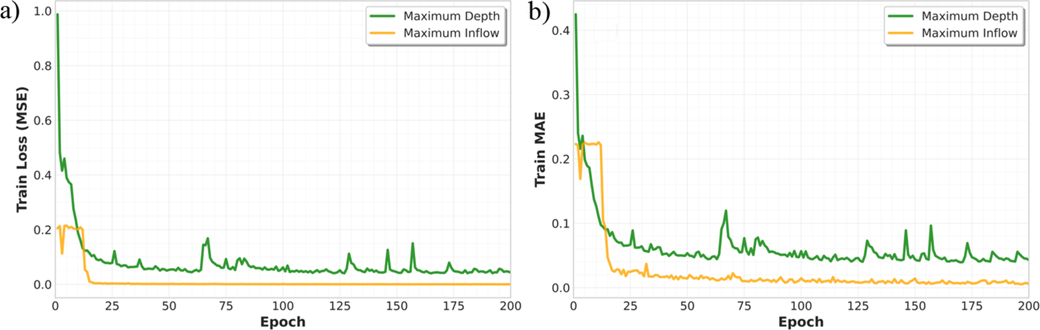
Figure 5 further illustrates the validation performance of the selected optimal LSTM configurations over 200 training epochs. For maximum inflow prediction, both validation loss and RMSE rapidly converged to low values, maintaining stability throughout training. In contrast, maximum water depth prediction exhibited a slower convergence and periodic spikes in error, indicating higher sensitivity to training fluctuations and possibly a more complex learning task.
(a) Training loss (MSE) and (b) training MAE over 200 training epochs for LSTM-based predictions of maximum water depth and maximum inflow.

These results underscore the importance of task-specific hyperparameter optimization in LSTM-based flood drainage prediction models. While both prediction tasks benefited from careful tuning, the distinct error convergence patterns and variability highlight that a single, universal architecture may not yield optimal performance for multiple hydrologic and hydraulic outputs. Instead, tailoring network depth, hidden size and regularization parameters to the physical characteristics and variability of each target variable can substantially enhance predictive accuracy and stability.
Modeling performance
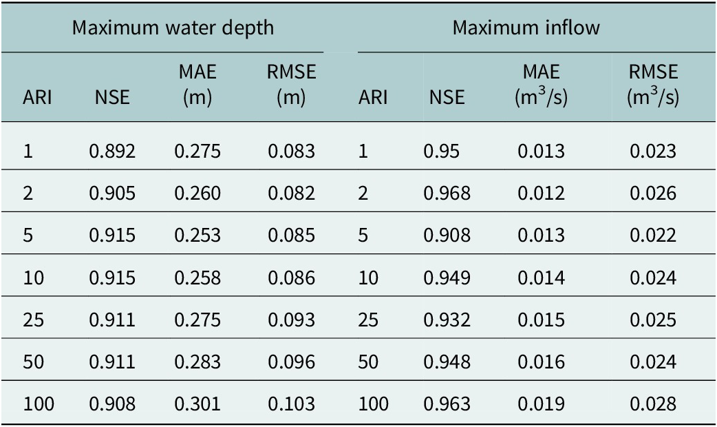
Table 2 summarizes the predictive performance of the optimal LSTM configurations for each target variable – maximum water depth and maximum inflow – across seven ARI categories (1, 2, 5, 10, 25, 50 and 100 years). For maximum water depth, NSE values range from 0.892 (ARI 1) to 0.915 (ARI 5 and 10), indicating strong modeling performance. Corresponding MAE values range between 0.253 and 0.301 m, while RMSE values remain low at 0.082–0.103 m. For maximum inflow, the model demonstrates higher accuracy, with NSE values ranging from 0.91 (ARI 5) to 0.97 (ARI 2), MAE values between 0.012 and 0.019 m3/s and RMSE values between 0.022 and 0.028 m3/s. Results show consistently high predictive skill for both variables, with inflow predictions achieving higher NSE values and lower error metrics compared to water depth. Quantitative performance metrics for the training and validation datasets are provided in Supplementary Table S2 of the Supporting Material, indicating consistent model behavior and satisfactory generalization for both maximum water depth and maximum inflow.
Performance of the LSTM-based surrogate model on the independent test set, evaluated across different ARIs

Note: The dataset of 5,000 synthetic storm events was randomly partitioned into 70% training, 15% validation and 15% testing subsets. Results reflect test-only metrics using NSE, MAE and RMSE computed between simulated and predicted maxima across all nodes. RMSE and MAE values are reported in meters (for water depth) and m3/s (for inflow).
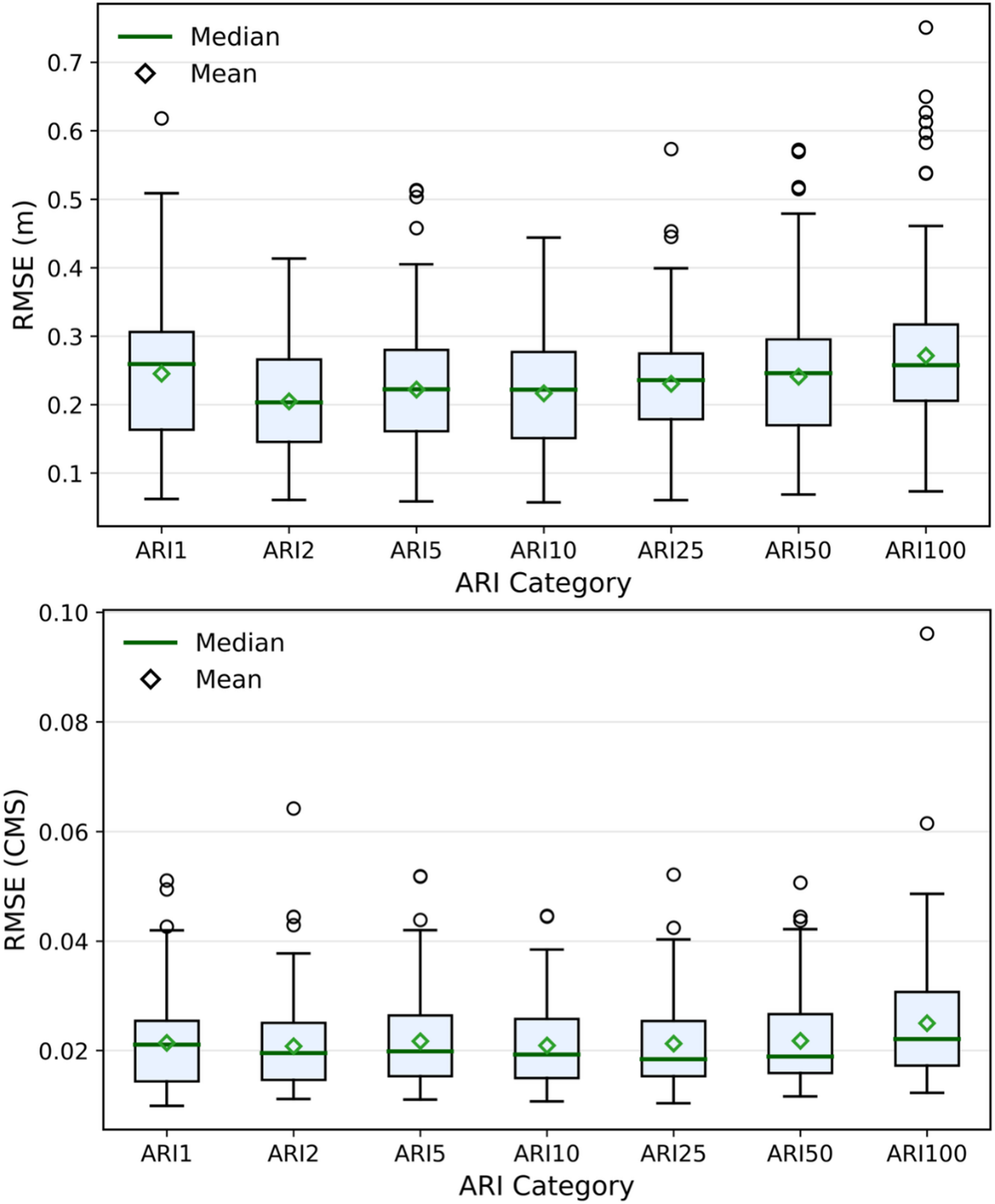
Figure 6 illustrates the RMSE of test dataset distribution for maximum water depth and maximum inflow across ARI categories. For water depth RMSE, variability increased slightly for higher ARI values, with ARI100 showing the largest spread and several high outliers, which suggested increased prediction difficulty under extreme events. For inflow RMSE, median and mean values remained consistently low across ARIs, though ARI100 again showed a marginal increase in variability. These results confirmed that while inflow predictions were generally more stable across return periods, water depth prediction accuracy was more sensitive to extreme rainfall intensities.
Boxplots of RMSE for LSTM-based predictions of maximum water depth (top) and maximum inflow (bottom) across seven ARI categories. Medians (green lines), means (green diamonds), interquartile ranges (boxes), data within 1.5× IQR (interquartile range; whiskers) and outliers (circles) are shown.

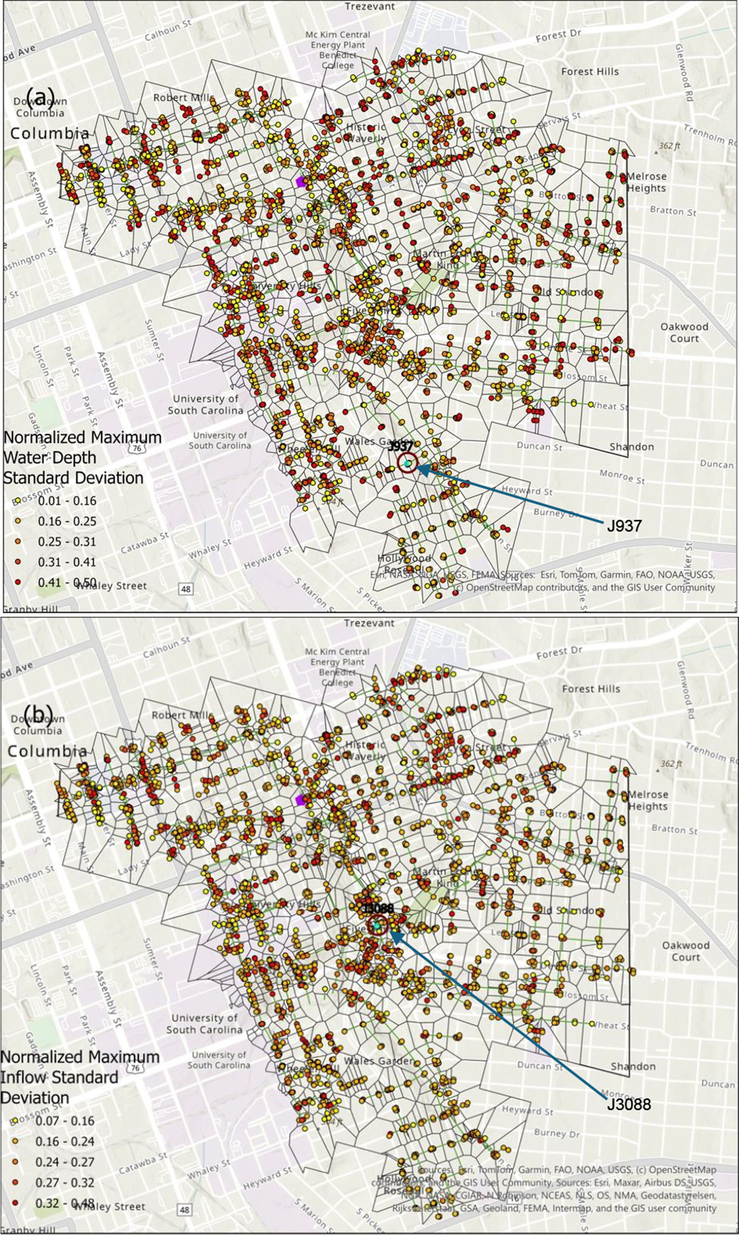
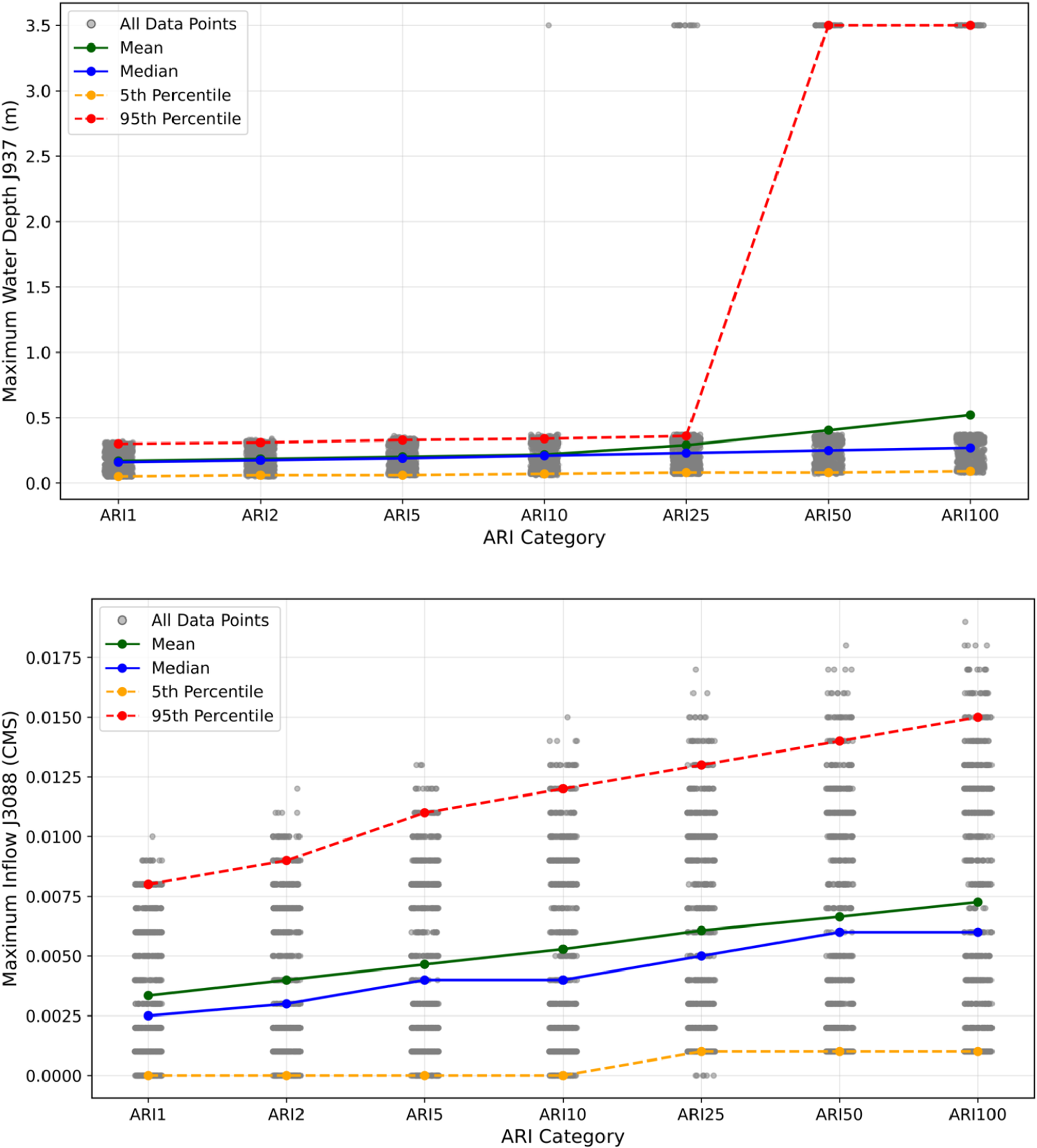
Figure 7 presents the spatial distribution of normalized standard deviation values for maximum water depth and maximum inflow across a network of junctions. Panel (a) showed the variability in maximum water depth, with color gradients ranging from 0.14 to 0.49. These values represent the standard deviation of the normalized peak depths computed across all 5,000 synthetic rainfall events, providing a spatial measure of inter-event variability. Junction J937 was highlighted as the location with the greatest change in water depth for further analysis. Panel (b) showed a similar distribution for normalized inflow variability, with Junction J3088 highlighted for its elevated variability in inflow. Figure 8 further investigates the temporal dynamics of two highlighted nodes: J937 and J3088. For each node, Figure 8 displays the distribution of maximum water depth and inflow, respectively, across multiple realizations for seven ARI categories ranging from ARI1 to ARI100, highlighting the highest inter-event variability.
Spatial distribution of inter-event variability across junctions for (a) normalized standard deviation of maximum water depth and (b) normalized standard deviation of maximum inflow, computed over all 5,000 synthetic rainfall events. Junctions J937 and J3088 are also illustrated.

Statistical analysis of maximum water depth and inflow across ARIs at junctions J937 and J3088, showing all data points, mean, median, 5th percentile and 95th percentile across ARI categories (1, 2, 5, 10, 25, 50 and 100 years).

At J937, water depth remained relatively stable across lower ARIs (i.e., ARI1–ARI10), but a distinct surge in variability emerged from ARI25 onward. The 95th percentile rose sharply, indicating outlier events with extreme water levels, likely driven by local topographic effects or system bottlenecks. Despite this upper-bound sensitivity, both median and mean remained comparatively stable, suggesting that only a limited number of scenarios produced disproportionately high depths. At J3088, inflow exhibited a more gradual and consistent increase with ARI. Both the mean and median rose consistently while the 5th–95th percentile range widened, reflecting heightened uncertainty under rarer, more extreme events. In contrast to J937, no sharp transition was observed, suggesting that inflow dynamics at this location were primarily governed by cumulative upstream contributions rather than localized nonlinear responses.
Together, these figures underscored the spatial and temporal heterogeneity of hydraulic response within the network. Identifying nodes with elevated variability is critical for prioritizing flood-mitigation interventions and designing adaptive capacity within urban drainage system.
Discussion and conclusion
This study demonstrates the effectiveness of the proposed spatiotemporal LSTM-based surrogate model in predicting event-level maxima of both water depth and inflow. To position the proposed surrogate within the broader literature on hybrid physics–ML frameworks, we compared characteristics of two recent LSTM–hydrodynamic models (Zhao et al., Reference Zhao, Liu, Li, Tang, Yang, Xu, Quan and Hu2023; Pan et al., Reference Pan, Hou, Gao, Chen, Li, Imran, Li, Yang, Ma and Zhou2025) alongside this study. Zhao et al. (Reference Zhao, Liu, Li, Tang, Yang, Xu, Quan and Hu2023) developed an LSTM–SWMM hybrid for outlet discharge prediction and reported NSE values of 0.969 for the hybrid model and 0.954 for a LSTM, with forecasting performance decreasing as the lead time increased. Pan et al. (Reference Pan, Hou, Gao, Chen, Li, Imran, Li, Yang, Ma and Zhou2025) used an LSTM trained on One-Dimensional–Two-Dimensional (1D–2D) hydrodynamic simulations to predict time series of inundation depth at a small number of flood-prone locations, achieving R 2 > 0.90, MAE ≤ 0.069 m and RMSE ≤0.077 m. In comparison, our SWMM-calibrated surrogate predicts event-level maxima of both depth and inflow at 2,802 junctions across seven ARIs, with NSE = 0.89–0.92 for maximum depth and 0.91–0.97 for maximum inflow, and low error statistics (depth RMSE ≤0.103 m, inflow RMSE ≤0.028 m3/s). Our framework extends previous hybrid approaches by (i) operating at the asset level across the entire drainage network rather than at a single outlet or a handful of inundation points, and (ii) providing comparable or better predictive skills while delivering event-scale forecasts suitable for real-time applications.
Model performance was rigorously evaluated across multiple ARIs, achieving consistently high predictive skill, with NSE values of up to 0.97 for inflow and 0.92 for water depth, alongside low error statistics. These results confirm the ability of recurrent deep networks to capture the nonlinear rainfall–runoff transformations inherent in urban hydrologic–hydraulic systems when trained on sufficiently diverse datasets. Importantly, the model aligns with the well-documented challenges of reproducing threshold behaviors in hydraulic systems, including surcharging, backwater effects and localized bottlenecks. These nonlinear responses are often triggered once system capacity is exceeded and tend to escalate rapidly under extreme storm events due to overwhelming upstream runoff. Such behaviors highlight the intrinsic difficulty of capturing abrupt state shifts in flow regimes, where small variations in boundary conditions can lead to disproportionately large impacts on water depth and inflow. The model’s partial sensitivity to these dynamics underscores both the promise and the limitations of data-driven approaches in representing complex hydraulic transitions that are highly dependent on network topology and localized storage–conveyance interactions.
Furthermore, the surrogate exhibited systematically higher accuracy for inflow than for water depth, a physically consistent outcome since local depth maxima are more sensitive to pressurization, minor–major system exchanges and localized energy losses at manholes and structures, whereas inflow reflects more spatially integrated upstream contributions and thus exhibits smoother dynamics. Building upon the work of Pan et al. (Reference Pan, Hou, Gao, Chen, Li, Imran, Li, Yang, Ma and Zhou2025) in using LSTM surrogates to pinpoint inundation hotspots, our approach advances the field by generating complete area-wide forecasts, a critical capability for hydrological assessment and policy development. Additionally, studies such as Roy et al. (Reference Roy, Goodall, McSpadden, Goldenberg and Schram2025) highlighted the effectiveness seq2seq LSTM models in capturing rapid, nonlinear flood responses in urban areas, supporting the computational efficiency and accuracy of our proposed approach for real-time applications. Chang et al. (Reference Chang, Yang and Chang2025) proposed a hybrid neural network–backpropagation neural network (CNN–BPNN) model that couples spatial feature extraction with temporal learning and achieved high accuracy for 10-min urban water-level forecasts (sewer: R 2 = 0.97, RMSE = 0.08 m; internal/external: R 2 = 0.99, RMSE = 0.06 m), complementing our LSTM-based framework for real-time flood control. The surrogate model required careful adjustment to achieve optimal predictive accuracy. Results from the grid search revealed that larger hidden sizes combined with moderate dropout improved LSTM-based water depth predictions, whereas two-layer architectures with minimal dropout were more effective for inflow predictions. This outcome reflects the distinct error landscapes of the two target variables: water depth estimation demands stronger regularization to prevent overfitting local nonlinearities, while inflow prediction benefits from greater network capacity and remains stable without dropout. These insights underscore the importance of task-specific hyperparameter optimization when applying DL to complex urban drainage systems.
Although this study focuses on deterministic performance metrics, the surrogate model inevitably inherits uncertainty from both rainfall inputs and SWMM calibration parameters. A full probabilistic treatment is beyond the scope of this work, but future extensions could benefit from incorporating stochastic surrogate models such as LSTM ensembles or Monte Carlo dropout (Tabas and Samadi, Reference Tabas and Samadi2022) to generate predictive variance and uncertainty bounds suitable for operational decision-making.
For the Rocky Branch watershed, a full SWMM dynamic-wave simulation required an average of ~118 min per storm, whereas the trained LSTM surrogate produced predictions for all 5,000 events in just 16 min. This drastic reduction in computational runtime is what enables real-time, rapid decisions during extreme events.
It should be noted that although the LSTM surrogate can ingest rainfall information sequentially and update its predictions as new data become available, the model is trained using complete storm sequences at the event level. Accordingly, predictions produced during real-time storms represent inferences based on partial inputs rather than explicitly trained instantaneous forecasts. Despite this distinction, the approach remains valuable for real-time applications by providing rapidly updated estimates of expected peak conditions.
The proposed LSTM-based surrogate model offers two distinct advantages for urban flood management. First, by using an asset-level calibrated SWMM as input for the surrogate model, the approach provides a computationally efficient pathway for real-time decision support, enabling rapid scenario screening and transparent identification of critical hotspots across the drainage network. Second, surrogate enables rapid, high-resolution predictions of maximum water depth and inflow, facilitating real-time decision support, efficient scenario analysis and transparent identification of flood hotspots for stakeholders. Unlike traditional SWMM simulations, which are computationally intensive and often impractical for real-time applications due to runtimes exceeding hours for large networks, our approach leverages precomputed SWMM output stored in metafiles (e.g., Excel files). These files archive time-series rainfall data alongside corresponding maximum depth and inflow results for each event, enabling the LSTM model to train on these datasets and deliver forecasts with exceptional speed. This efficiency is critical for emergency response during extreme events, empowering communities and authorities with timely, actionable insights to mitigate flood impacts. By combining strong predictive accuracy with orders-of-magnitude faster computation, the developed surrogate offers a practical, scalable tool that supports flood mitigation, urban planning and community resilience under increasingly extreme rainfall events.
Open peer review
To view the open peer review materials for this article, please visit http://doi.org/10.1017/wat.2026.10013.
Supplementary material
The supplementary material for this article can be found at http://doi.org/10.1017/wat.2026.10013.
Data availability statement
The discharge data were obtained from the USGS gauge Rocky Branch at Pickens St. in Columbia, SC (Station 02169505; https://waterdata.usgs.gov/monitoring-location/USGS-02169505/). Rainfall data were obtained from https://waterdata.usgs.gov/monitoring-location/USGS-021695045, and drainage network layers were provided by the City of Columbia’s GIS portal (https://gis.columbiasc.gov) upon request for academic research.
Author contribution
Nima Zafarmomen: Writing – original draft, visualization, validation, software, methodology, formal analysis and conceptualization.
Vidya Samadi: Writing – review and editing, validation, supervision, project administration, methodology, funding acquisition and conceptualization.
Edoardo Borgomeo: Writing – review and editing, validation, supervision and methodology.
Financial support
This work is supported by the US National Science Foundation (NSF) Directorate for Engineering under grant CBET 2429082. Clemson University (USA) is acknowledged for its generous allotment of computing time on the Palmetto cluster. EB is supported by INT/UCam Early Career Support Scheme (Award number G122390).
Competing interests
The authors declare none.


 Open access
Comments
9/27/2025
Dear Prof. Fenner,
Editor in Chief of Cambridge Prisms: Water
On behalf of my coauthor, I wish to request your consideration of our research article titled “Spatiotemporal SWMM-LSTM Surrogate Modeling for Efficient Node-Level Water Depth and Inflow Prediction in Urban Drainage Networks” for publication in Cambridge Prisms: Water. This project is the result of a US National Science Foundation-funded project.
This study presents a novel hybrid modeling framework that integrates high-resolution, asset-level calibration of the EPA’s SWMM with spatiotemporal Long Short-Term Memory (LSTM) networks. We believe this work aligns closely with the journal’s focus on innovative water research and management strategies, particularly in urban flood risk modeling and smart water systems. Our study provides a scalable, adaptable framework that can inform resilient urban planning and climate-responsive infrastructure development.
We confirm that this manuscript has not been published elsewhere and is not under consideration by any other journal. All authors have approved the submission and declare no competing interests. Thank you very much for your consideration. We look forward to your feedback and hope that our work will contribute to advancing research in urban water management.
Sincerely,
Vidya Samadi, Ph.D., M.ASCE.
Assistant Professor & Director of Clemson Hydroinformatics Research Group,
Affiliate Faculty, Artificial Intelligence Research Institute for Science and Engineering (AIRISE), School of Computing Clemson University, SC, USA.